ms1b statistical machine learning and data miningteh/teaching/smldmht2014/w1slides.pdf ·...
TRANSCRIPT

MS1bStatistical Machine Learning and Data Mining
Yee Whye TehDepartment of Statistics
Oxford
http://www.stats.ox.ac.uk/~teh/smldm.html
1

Course Information
� Course webpage:http://www.stats.ox.ac.uk/~teh/smldm.html
� Lecturer: Yee Whye Teh� TA for Part C: Thibaut Lienant� TA for MSc: Balaji Lakshminarayanan and Maria Lomeli� Please subscribe to Google Group:
https://groups.google.com/forum/?hl=en-GB#!forum/smldm
� Sign up for course using sign up sheets.
2

Course StructureLectures
� 1400-1500 Mondays in Math Institute L4.� 1000-1100 Wednesdays in Math Institute L3.
Part C:� 6 problem sheets.� Classes: 1600-1700 Tuesdays (Weeks 3-8) in 1 SPR Seminar Room.� Due Fridays week before classes at noon in 1 SPR.
MSc:� 4 problem sheets.� Classes: Tuesdays (Weeks 3, 5, 7, 9) in 2 SPR Seminar Room.� Group A: 1400-1500, Group B: 1500-1600.� Due Fridays week before classes at noon in 1 SPR.� Practical: Week 5 and 7 (assessed) in 1 SPR Computing Lab.� Group A: 1400-1600, Group B: 1600-1800.
3

Course Aims
1. Have ability to use the relevant R packages to analyse data, interpretresults, and evaluate methods.
2. Have ability to identify and use appropriate methods and models for givendata and task.
3. Understand the statistical theory framing machine learning and datamining.
4. Able to construct appropriate models and derive learning algorithms forgiven data and task.
4

What is Machine Learning?
sensory
What's out there?How does world work?
What's going to happen?What should i do?
data
5

What is Machine Learning?
data
InformationStructurePredictionDecisionsActions
http://gureckislab.org 6

What is Machine Learning?
Machine Learning
statistics
computerscience
cognitivescience
psychology
mathematics
engineeringoperationsresearch
physics
biologygenetics
businessfinance
7

What is the Difference?
Traditional Problems in Applied StatisticsWell formulated question that we would like to answer.Expensive to gathering data and/or expensive to do computation.Create specially designed experiments to collect high quality data.
Current SituationInformation Revolution
� Improvements in computers and data storage devices.� Powerful data capturing devices.� Lots of data with potentially valuable information available.
8
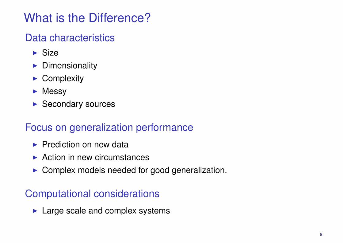
What is the Difference?Data characteristics
� Size� Dimensionality� Complexity� Messy� Secondary sources
Focus on generalization performance� Prediction on new data� Action in new circumstances� Complex models needed for good generalization.
Computational considerations� Large scale and complex systems
9

Applications of Machine Learning
� Pattern Recognition
� Sorting Cheques� Reading License Plates� Sorting Envelopes� Eye/ Face/ Fingerprint Recognition
10

Applications of Machine Learning
� Business applications� Help companies intelligently find information� Credit scoring� Predict which products people are going to buy� Recommender systems� Autonomous trading
� Scientific applications� Predict cancer occurence/type and health of patients/personalized health� Make sense of complex physical, biological, ecological, sociological models
11

Further Readings, News and Applications
Links are clickable in pdf. More recent news posted on course webpage.� Leo Breiman: Statistical Modeling: The Two Cultures� NY Times: R� NY Times: Career in Statistics� NY Times: Data Mining in Walmart� NY Times: Big Data’s Impact In the World� Economist: Data, Data Everywhere� McKinsey: Big data: The Next Frontier for Competition� NY Times: Scientists See Promise in Deep-Learning Programs� New Yorker: Is “Deep Learning” a Revolution in Artificial Intelligence?
12

Types of Machine Learning
Unsupervised LearningUncover structure hidden in ‘unlabelled’ data.
� Given network of social interactions, find communities.� Given shopping habits for people using loyalty cards: find groups of
‘similar’ shoppers.� Given expression measurements of 1000s of genes for 1000s of patients,
find groups of functionally similar genes.
Goal: Hypothesis generation, visualization.
13
Types of Machine Learning
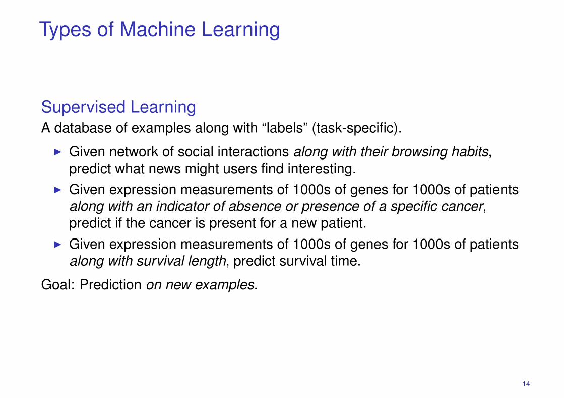
Supervised LearningA database of examples along with “labels” (task-specific).
� Given network of social interactions along with their browsing habits,predict what news might users find interesting.
� Given expression measurements of 1000s of genes for 1000s of patientsalong with an indicator of absence or presence of a specific cancer,predict if the cancer is present for a new patient.
� Given expression measurements of 1000s of genes for 1000s of patientsalong with survival length, predict survival time.
Goal: Prediction on new examples.
14

Types of Machine Learning
Semi-supervised LearningA database of examples, only a small subset of which are labelled.
Multi-task LearningA database of examples, each of which has multiple labels corresponding todifferent prediction tasks.
Reinforcement LearningAn agent acting in an environment, given rewards for performing appropriateactions, learns to maximize its reward.
15

OxWaSP
Oxford-Warwick Centre for Doctoral Training in Statistics� Programme aims to produce EuropeÕs future research leaders in
statistical methodology and computational statistics for modernapplications.
� 10 fully-funded (UK, EU) students a year (1 international).� Website for prospective students.� Deadline: January 24, 2014
16

Exploratory Data Analysis
Notation� Data consists of p measurements (variables/attributes) on n examples
(observations/cases)� X is a n × p-matrix with Xij := the j-th measurement for the i-th example
X =
x11 x12 . . . x1j . . . x1px21 x22 . . . x2j . . . x2p...
.... . .
.... . .
...xi1 xi2 . . . xij . . . xip...
.... . .
.... . .
...xn1 xn2 . . . xnj . . . xnp
� Denote the ith data item by xi ∈ Rp. (This is transpose of ith row of X)
� Assume x1, . . . , xn are independently and identically distributed samplesof a random vector X over Rp.
17

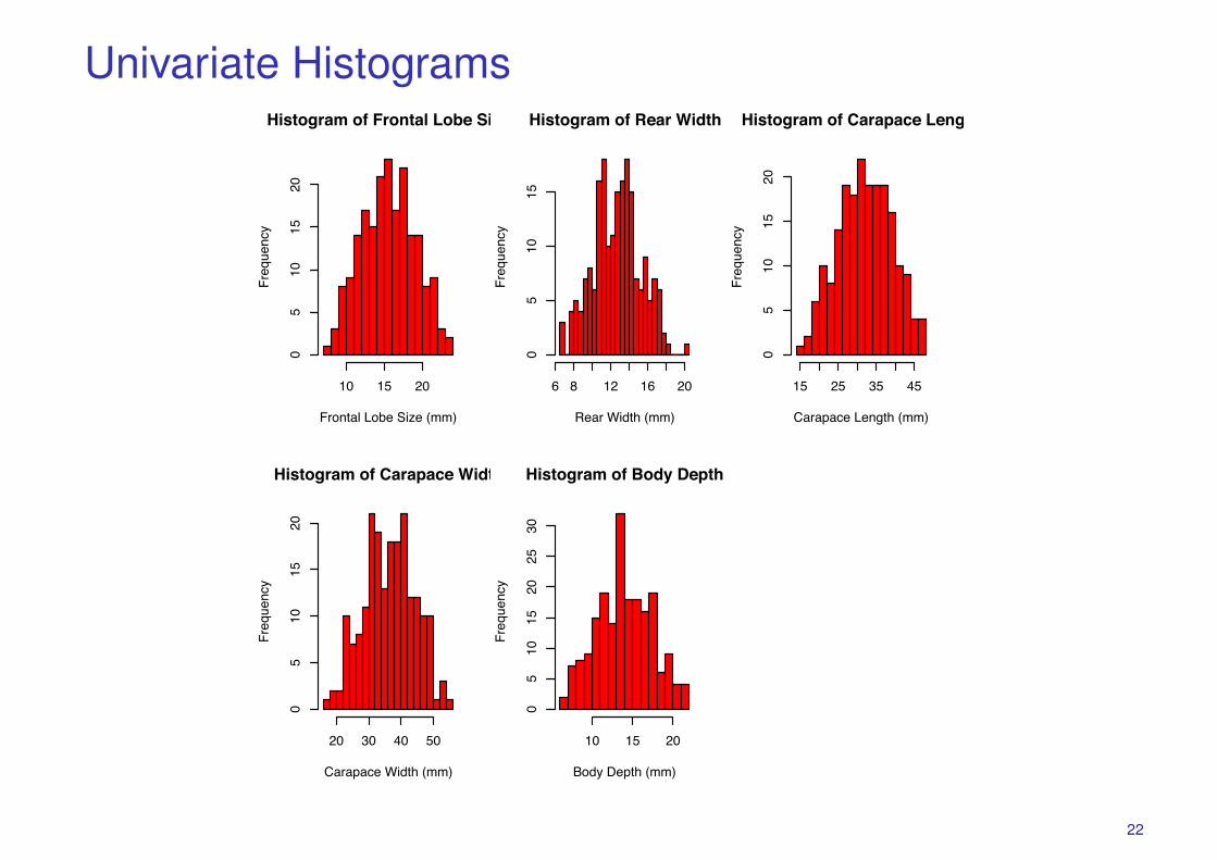
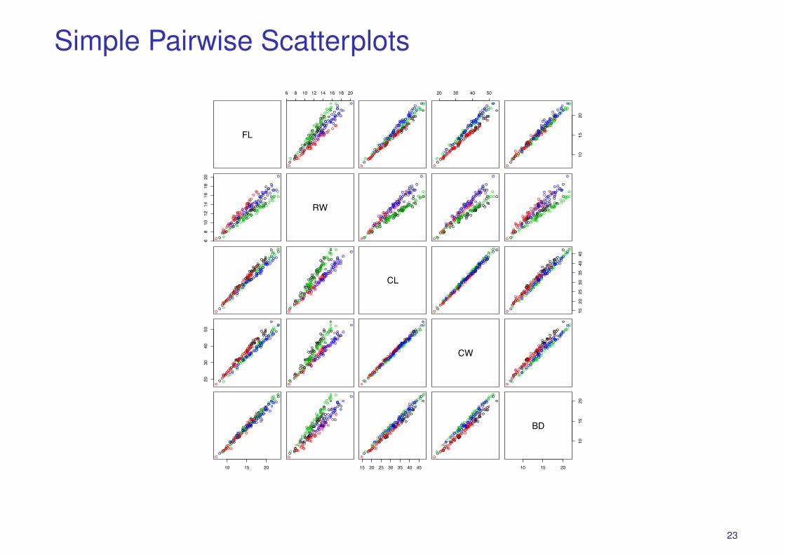
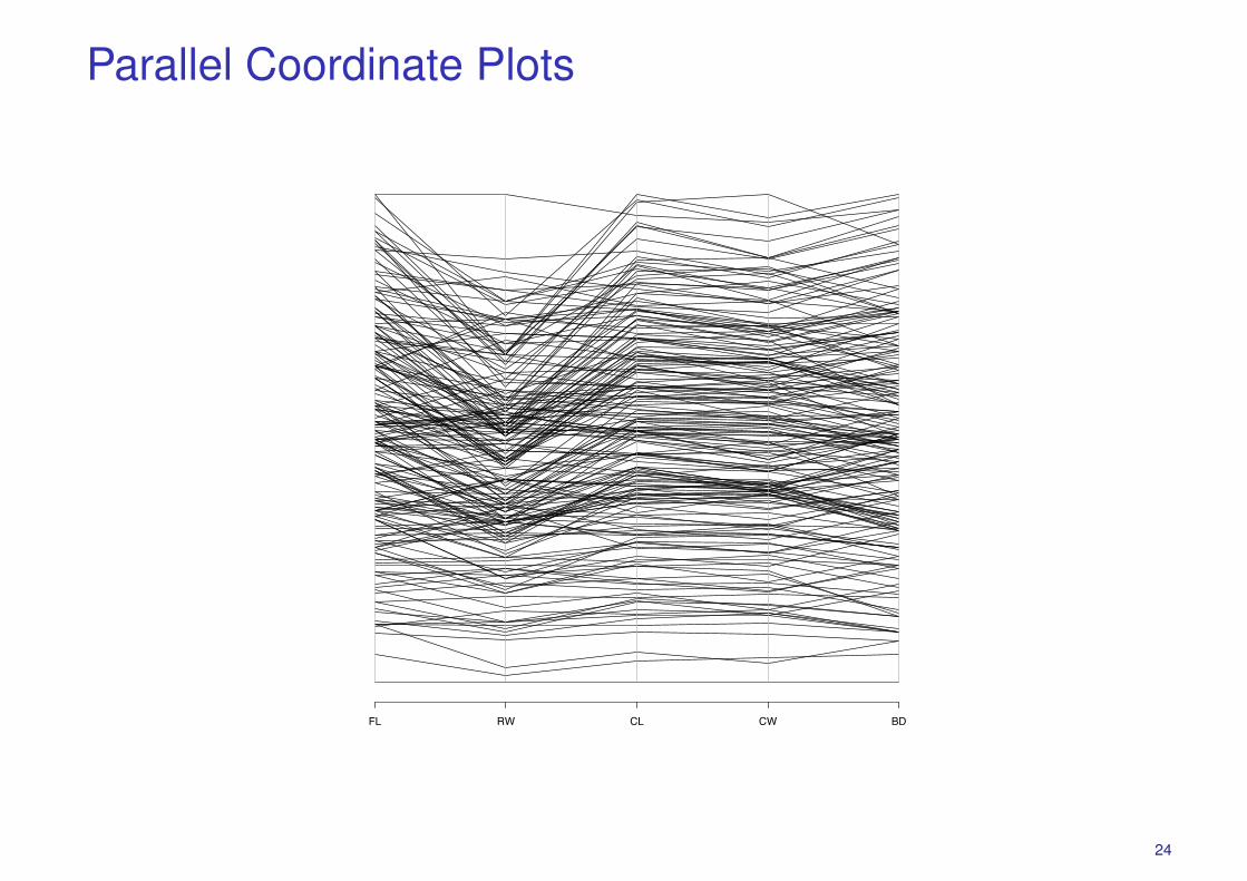
Crabs Data (n = 200, p = 5)
Campbell (1974) studied rock crabs of the genus leptograpsus. One species,L. variegatus, had been split into two new species, previously grouped bycolour, orange and blue. Preserved specimens lose their colour, so it washoped that morphological differences would enable museum material to beclassified.
Data are available on 50 specimens of each sex of each species, collected onsight at Fremantle, Western Australia. Each specimen has measurements on:
� the width of the frontal lobe FL,� the rear width RW,� the length along the carapace midline CL,� the maximum width CW of the carapace, and� the body depth BD in mm.
in addition to colour (species) and sex.
18
Crabs Data I
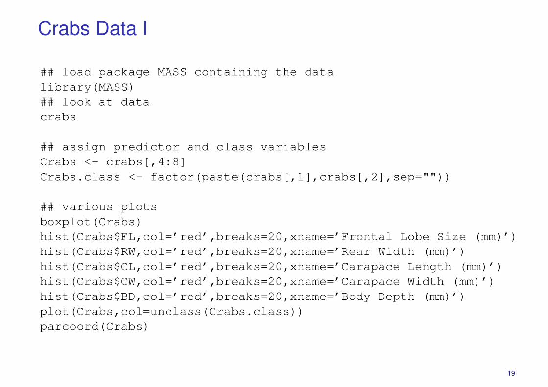
## load package MASS containing the datalibrary(MASS)## look at datacrabs
## assign predictor and class variablesCrabs <- crabs[,4:8]Crabs.class <- factor(paste(crabs[,1],crabs[,2],sep=""))
## various plotsboxplot(Crabs)hist(Crabs$FL,col=’red’,breaks=20,xname=’Frontal Lobe Size (mm)’)hist(Crabs$RW,col=’red’,breaks=20,xname=’Rear Width (mm)’)hist(Crabs$CL,col=’red’,breaks=20,xname=’Carapace Length (mm)’)hist(Crabs$CW,col=’red’,breaks=20,xname=’Carapace Width (mm)’)hist(Crabs$BD,col=’red’,breaks=20,xname=’Body Depth (mm)’)plot(Crabs,col=unclass(Crabs.class))parcoord(Crabs)
19
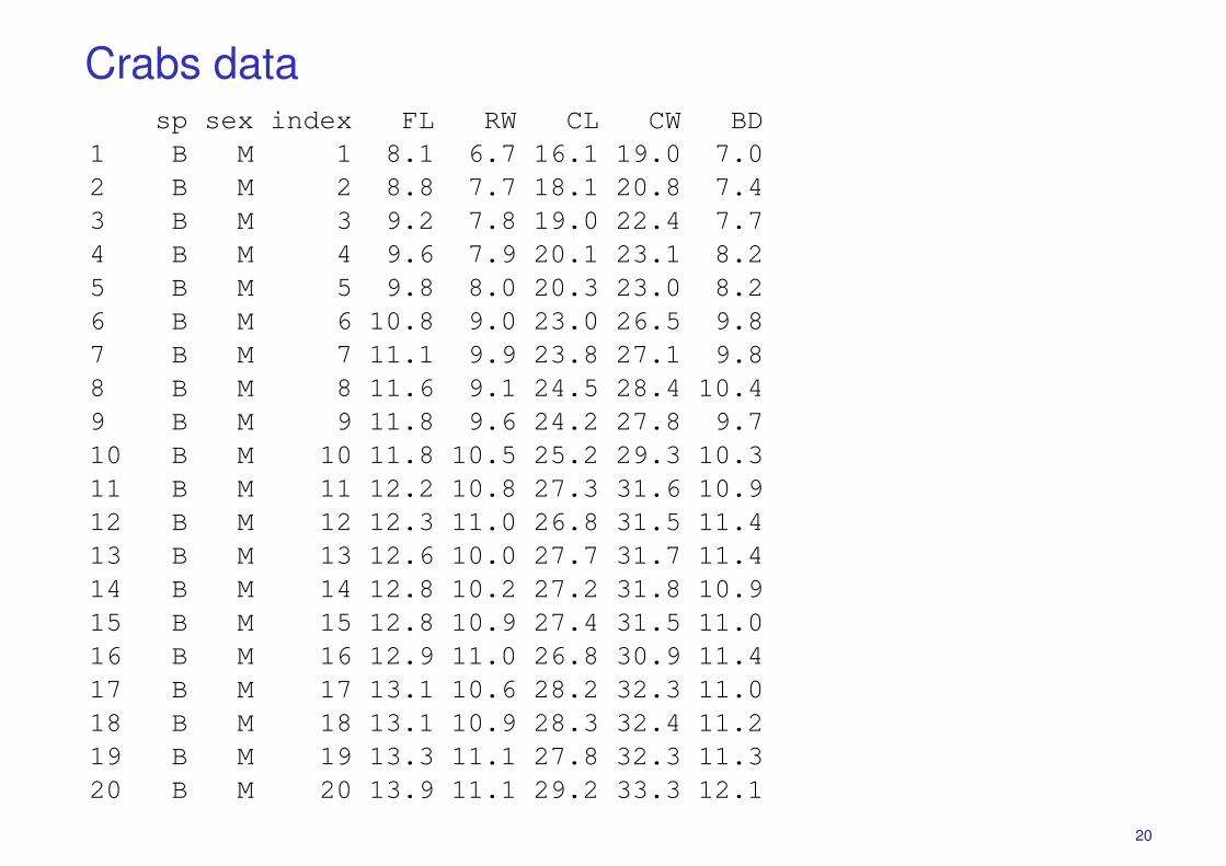
Crabs datasp sex index FL RW CL CW BD
1 B M 1 8.1 6.7 16.1 19.0 7.02 B M 2 8.8 7.7 18.1 20.8 7.43 B M 3 9.2 7.8 19.0 22.4 7.74 B M 4 9.6 7.9 20.1 23.1 8.25 B M 5 9.8 8.0 20.3 23.0 8.26 B M 6 10.8 9.0 23.0 26.5 9.87 B M 7 11.1 9.9 23.8 27.1 9.88 B M 8 11.6 9.1 24.5 28.4 10.49 B M 9 11.8 9.6 24.2 27.8 9.710 B M 10 11.8 10.5 25.2 29.3 10.311 B M 11 12.2 10.8 27.3 31.6 10.912 B M 12 12.3 11.0 26.8 31.5 11.413 B M 13 12.6 10.0 27.7 31.7 11.414 B M 14 12.8 10.2 27.2 31.8 10.915 B M 15 12.8 10.9 27.4 31.5 11.016 B M 16 12.9 11.0 26.8 30.9 11.417 B M 17 13.1 10.6 28.2 32.3 11.018 B M 18 13.1 10.9 28.3 32.4 11.219 B M 19 13.3 11.1 27.8 32.3 11.320 B M 20 13.9 11.1 29.2 33.3 12.1
20
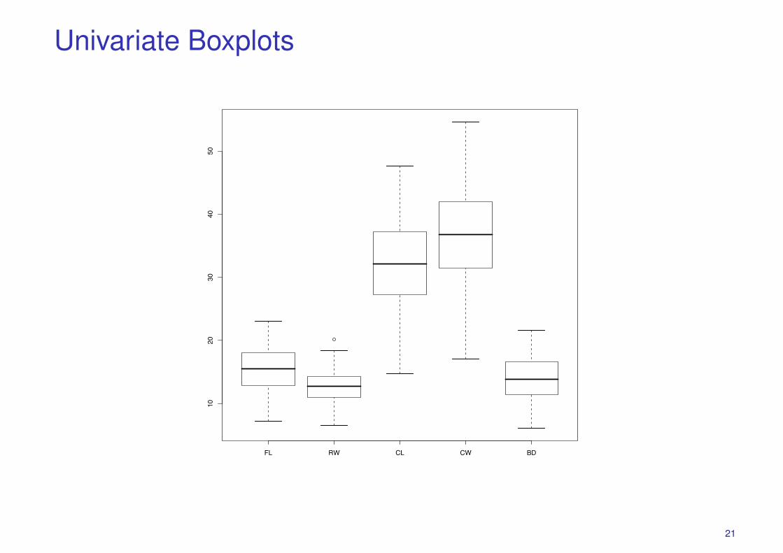
Univariate Boxplots
FL RW CL CW BD
1020
3040
50
21
Univariate HistogramsHistogram of Frontal Lobe Size
Frontal Lobe Size (mm)
Freq
uenc
y
10 15 20
05
1015
20
Histogram of Rear Width
Rear Width (mm)
Freq
uenc
y
6 8 12 16 20
05
1015
Histogram of Carapace Length
Carapace Length (mm)
Freq
uenc
y
15 25 35 45
05
1015
20
Histogram of Carapace Width
Carapace Width (mm)
Freq
uenc
y
20 30 40 50
05
1015
20
Histogram of Body Depth
Body Depth (mm)
Freq
uenc
y
10 15 20
05
1015
2025
30
22
Simple Pairwise Scatterplots
FL
6 8 10 12 14 16 18 20 20 30 40 50
1015
20
68
1012
1416
1820
RW
CL
1520
2530
3540
45
2030
4050
CW
10 15 20 15 20 25 30 35 40 45 10 15 20
1015
20
BD
23
Parallel Coordinate Plots
FL RW CL CW BD
24
Visualization and Dimensionality Reduction
These summary plots are helpful, but do not really help very much if thedimensionality of the data is high (a few dozen or thousands).Visualizing higher-dimensional problems:
� We are constrained to view data in 2 or 3 dimensions� Look for ‘interesting’ projections of X into lower dimensions� Hope that for large p, considering only k � p dimensions is just as
informative.
Dimensionality reduction� For each data item xi ∈ R
p, find a lower dimensional representationzi ∈ R
k with k � p.� Preserve as much as possible the interesting statistical
properties/relationships of data items.
25

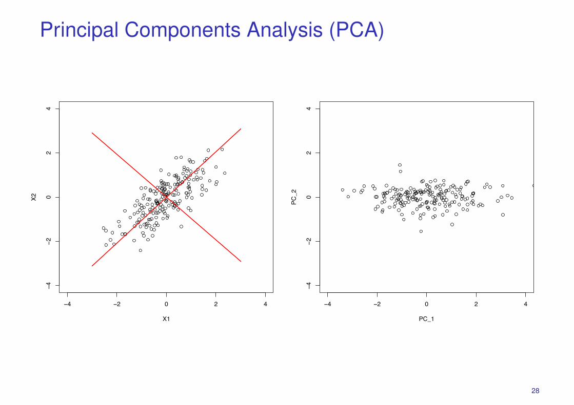
Principal Components Analysis (PCA)
� PCA considers interesting directions to be those with greatest variance.� A linear dimensionality reduction technique:� Finds an orthogonal basis v1, v2, . . . , vp for the data space such that
� The first principal component (PC) v1 is the direction of greatest variance ofdata.
� The second PC v2 is the direction orthogonal to v1 of greatest variance, etc.� The subspace spanned by the first k PCs represents the ’best’ k-dimensional
representation of the data.� The k-dimensional representation of xi is:
zi = V�xi =k�
�=1
v�� xi
where V ∈ Rp×k.
� For simplicity, we will assume from now on that our dataset is centred, i.e.we subtract the average x̄ from each xi.
26
Principal Components Analysis (PCA)
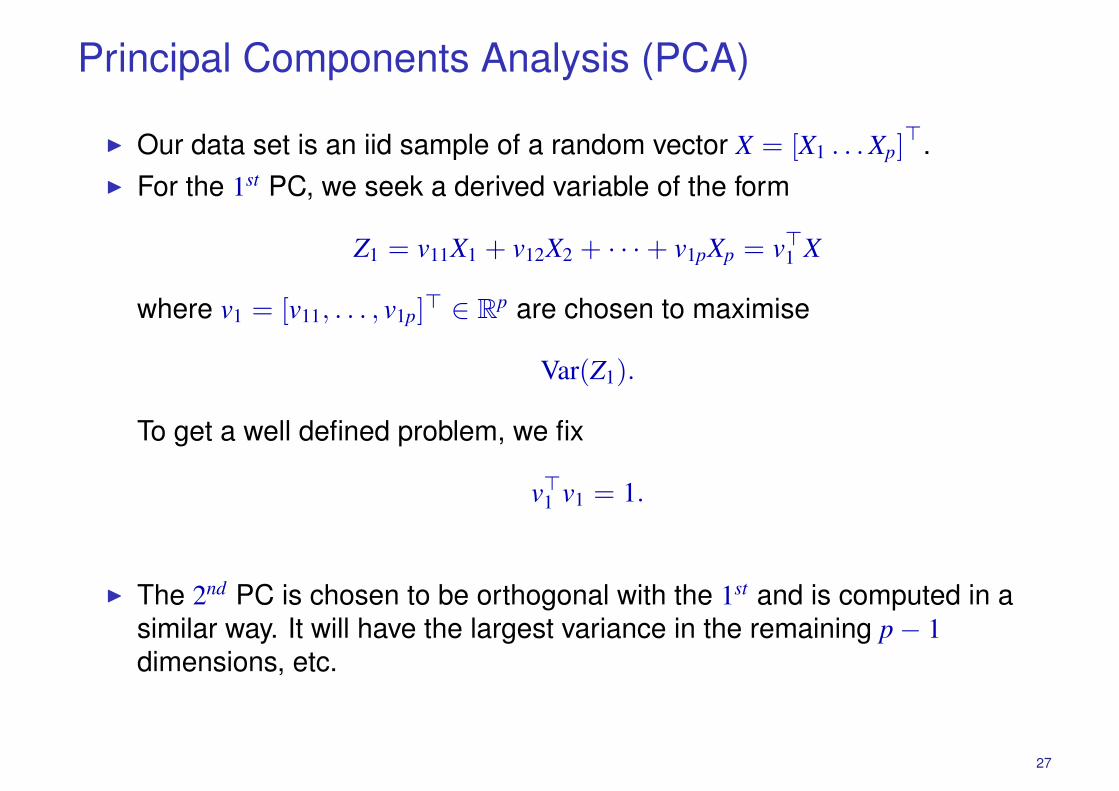
� Our data set is an iid sample of a random vector X = [X1 . . .Xp]�.
� For the 1st PC, we seek a derived variable of the form
Z1 = v11X1 + v12X2 + · · ·+ v1pXp = v�1 X
where v1 = [v11, . . . , v1p]� ∈ Rp are chosen to maximise
Var(Z1).
To get a well defined problem, we fix
v�1 v1 = 1.
� The 2nd PC is chosen to be orthogonal with the 1st and is computed in asimilar way. It will have the largest variance in the remaining p − 1dimensions, etc.
27
Principal Components Analysis (PCA)
−4 −2 0 2 4
−4−2
02
4
X1
X2
−4 −2 0 2 4−4
−20
24
PC_1
PC_2
28

Deriving the First Principal Component� Maximise, subject to v�1 v1 = 1:
Var(Z1) = Var(v�1 X) = v�1 Cov(X)v1 ≈ v�1 Sv1
where S ∈ Rp×p is the sample covariance matrix, i.e.
S =1
n − 1
n�
i=1
(xi − x̄)(xi − x̄)� =1
n − 1
n�
i=1
xix�i =1
n − 1X�X.
� Rewriting this as a constrained maximisation problem,
L (v1,λ1) = v�1 Sv1 − λ1�v�1 v1 − 1
�.
� The corresponding vector of partial derivatives yields∂L(v1,λ1)
∂v1= 2Sv1 − 2λ1v1.
� Setting this to zero reveals the eigenvector equation, i.e. v1 must be aneigenvector of S and λ1 the corresponding eigenvalue.
� Since v�1 Sv1 = λ1v�1 v1 = λ1, the 1st PC must be the eigenvectorassociated with the largest eigenvalue of S.
29

Deriving Subsequent Principal Components� Proceed as before but include the additional constraint that the 2nd PC
must be orthogonal to the 1st PC:
L (v2,λ2, µ) = v�2 Sv2 − λ2�v�2 v2 − 1
�− µ
�v�1 v2
�.
� Solving this shows that v2 must be the eigenvector of S associated withthe 2nd largest eigenvalue, and so on
� The eigenvalue decomposition of S is given by
S = VΛV�
where Λ is a diagonal matrix with eigenvalues
λ1 ≥ λ2 ≥ · · · ≥ λp ≥ 0
and V is a p × p orthogonal matrix whose columns are the p eigenvectorsof S, i.e. the principal components v1, . . . , vp.
30
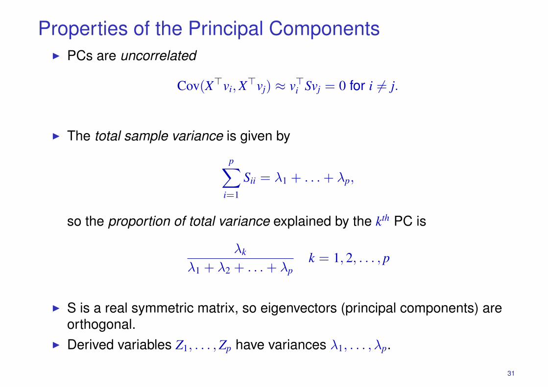
Properties of the Principal Components� PCs are uncorrelated
Cov(X�vi,X�vj) ≈ v�i Svj = 0 for i �= j.
� The total sample variance is given by
p�
i=1
Sii = λ1 + . . .+ λp,
so the proportion of total variance explained by the kth PC is
λk
λ1 + λ2 + . . .+ λpk = 1, 2, . . . , p
� S is a real symmetric matrix, so eigenvectors (principal components) areorthogonal.
� Derived variables Z1, . . . , Zp have variances λ1, . . . ,λp.
31

R code
This is what we have had before:
library(MASS)Crabs <- crabs[,4:8]Crabs.class <- factor(paste(crabs[,1],crabs[,2],sep=""))plot(Crabs,col=unclass(Crabs.class))
Now perform PCA with function princomp. (Alternatively, solve for the PCsyourself using eigen or svd).
Crabs.pca <- princomp(Crabs,cor=FALSE)plot(Crabs.pca)pairs(predict(Crabs.pca),col=unclass(Crabs.class))
32

Original Crabs Data
FL
6 8 10 12 14 16 18 20 20 30 40 50
1015
20
68
1012
1416
1820
RW
CL
1520
2530
3540
45
2030
4050
CW
10 15 20 15 20 25 30 35 40 45 10 15 20
1015
20
BD
33
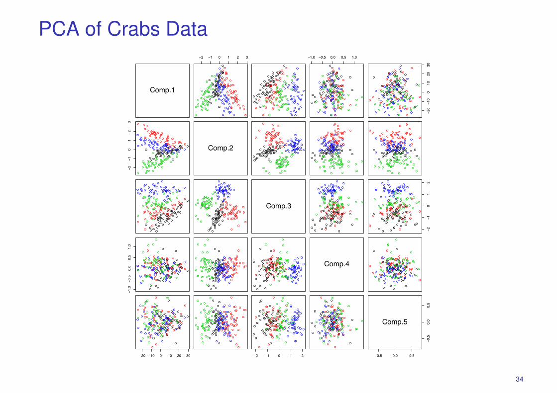
PCA of Crabs Data
Comp.1
−2 −1 0 1 2 3 −1.0 −0.5 0.0 0.5 1.0
−20
−10
010
2030
−2−1
01
23
Comp.2
Comp.3
−2−1
01
2
−1.0
−0.5
0.0
0.5
1.0
Comp.4
−20 −10 0 10 20 30 −2 −1 0 1 2 −0.5 0.0 0.5
−0.5
0.0
0.5
Comp.5
34
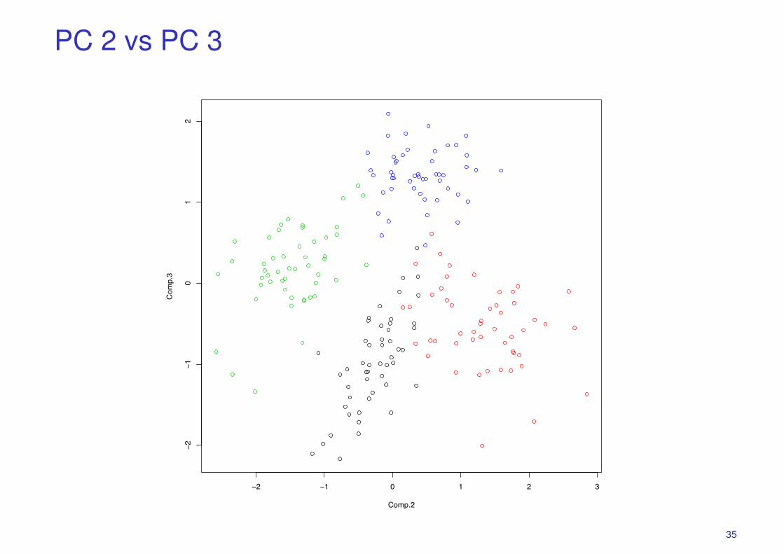
PC 2 vs PC 3
−2 −1 0 1 2 3
−2−1
01
2
Comp.2
Com
p.3
35
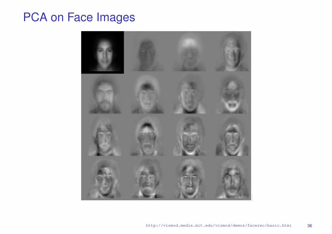
PCA on Face Images
http://vismod.media.mit.edu/vismod/demos/facerec/basic.html 36
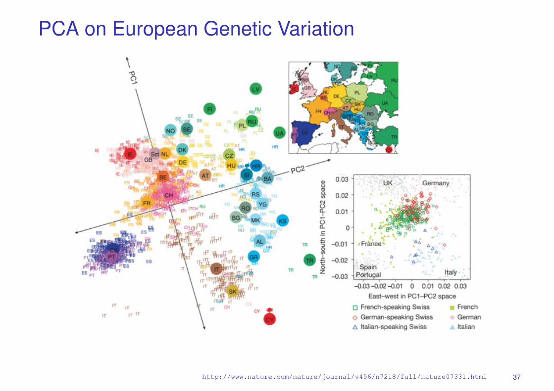
PCA on European Genetic Variation
http://www.nature.com/nature/journal/v456/n7218/full/nature07331.html 37
Comments on the use of PCA
� PCA commonly used to project data X onto the first k PCs giving thek-dimensional view of the data that best preserves the first two moments.
� Although PCs are uncorrelated, scatterplots sometimes reveal structuresin the data other than linear correlation.
� PCA commonly used for lossy compression of high dimensional data.� Emphasis on variance is where the weaknesses of PCA stem from:
� The PCs depend heavily on the units measurement. Where the data matrixcontains measurements of vastly differing orders of magnitude, the PC willbe greatly biased in the direction of larger measurement. It is thereforerecommended to calculate PCs from Corr(X) instead of Cov(X).
� Robustness to outliers is also an issue. Variance is affected by outlierstherefore so are PCs.
38
Eigenvalue Decomposition (EVD)
Eigenvalue decomposition plays a significant role in PCA. PCs areeigenvectors of S = 1
n−1 X�X and PCA properties are derived from those ofeigenvectors and eigenvalues.
� For any p × p symmetric matrix S, there exists p eigenvectors v1, . . . , vpthat are pairwise orthogonal and p associated eigenvalues λ1, . . . ,λpwhich satisfy the eigenvalue equation Svi = λivi ∀i.
� S can be written as S = VΛV� where� V = [v1, . . . , vp] is a p × p orthogonal matrix� Λ = diag {λ1, . . . ,λp}� If S is a real-valued matrix, then the eigenvalues are real-valued as well,
λi ∈ R ∀i� To compute the PCA of a dataset X, we can:
� First estimate the covariance matrix using the sample covariance S.� Compute the EVD of S using the R command eigen.
39
Singular Value Decomposition (SVD)
Though the EVD does not always exist, the singular value decomposition isanother matrix factorization technique that always exist, even for non-squarematrices.
� X can be written as X = UDV� where� U is an n × n matrix with orthogonal columns.� D is a n × p matrix with decreasing non-negative elements on the diagonal
(the singular values) and zero off-diagonal elements.� V is a p × p matrix with orthogonal columns.
� SVD can be computed using very fast and numerically stable algorithms.The relevant R command is svd.
40

Some Properties of the SVD� Let X = UDV� be the SVD of the n × p data matrix X.� Note that
(n − 1)S = X�X = (UDV�)�(UDV�) = VD�U�UDV� = VD�DV�,
using orthogonality (U�U = In) of U.� The eigenvalues of S are thus the diagonal entries of 1
n−1 D2 and thecolumns of the orthogonal matrix V are the eigenvectors of S.
� We also have
XX� = (UDV�)(UDV�)� = UDV�VD�U� = UDD�U�,
using orthogonality (V�V = Ip) of V.� SVD also gives the optimal low-rank approximations of X:
minX̃
�X̃ − X�2 s.t. X̃ has maximum rank r < n, p.
This problem can be solved by keeping only the r largest singular valuesof X, zeroing out the smaller singular values in the SVD.
41

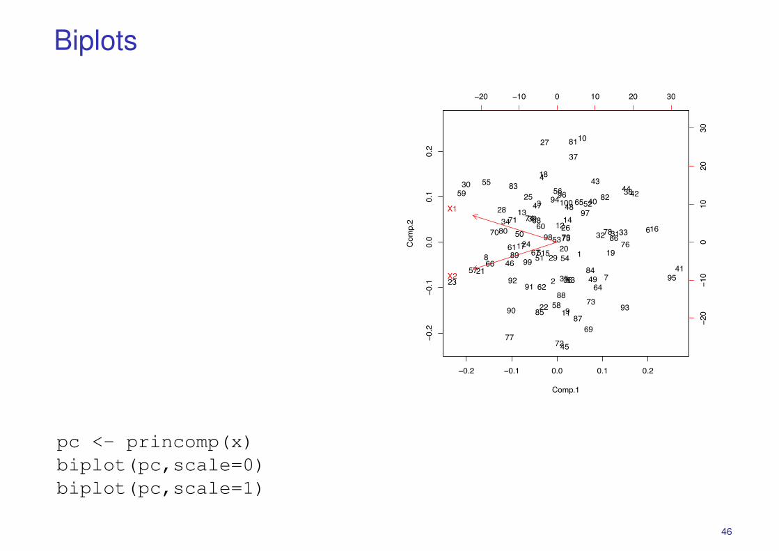
Biplots
� PCA plots show the data items (as rows of X) in the PC space.� Biplots allow us to visualize the original variables (as columns X) in the
same plot.� As for PCA, we would like the geometry of the plot to preserve as much
of the covariance structure as possible.
42

BiplotsRecall that X = [X1, . . . ,Xp]� and X = UDV� is the SVD of the data matrix.
� The PC projection of xi is:
zi = V�xi = DU�
i = [D11Ui1, . . . ,DkkUik]�.
� The jth unit vector ej ∈ Rp points in the direction of Xj. Its PC projection is
V�j = V�ej, the jth row of V.
� The projection of the variable indicates the weighting each PC gives tothe original variables.
� Dot products between the projections gives entries of the data matrix:
xij =p�
k=1
UikDkkVjk = �DU�
i ,V�
j �.
� Distance of projected points from projected variables gives originallocation.
� These relationships can be plotted in 2D by focussing on first two PCs.
43

Biplots
●
●
●
●
●
●
●
●
●
●
●
●
●
●
●
●
●
●
●
●
●
●
●
●
●
●
●
●
●
●
●
●
●
●
●●
●
●
●
●
●
●
●
●
●
●
●
●●
●
●
●
●●
●
●
●
●
●
●
●
●
●
●
●
●
●
●
●
●
●
●
●
●
●
●
●
●
●
●
●
●
●
●
●
●
●
●
●
●
●
●
●
●
●
●
●
●
●
●
−5 0 5
−6−4
−20
24
6
X1
X2
44

Biplots� There are other projections we can consider for biplots:
xij =p�
k=1
UikDkkVjk = �DU�
i ,V�
j � = �D1−αU�
i ,DαV�
j �.
where 0 ≤ α ≤ 1. The α = 1 case has some nice properties.� Covariance of the projected points is:
1n − 1
n�
i=1
U�
i Ui =1
n − 1I.
Projected points are uncorrelated and dimensions are equi-variance.� The covariance between Xj and X� is:
Var(XjX�) =1
n − 1�DV�
j ,DV�
� �
So the angle between the projected variables gives the correlation.� When using k < p PCs, quality depends on the proportion of variance
explained by the PCs.45
Biplots
−0.2 −0.1 0.0 0.1 0.2
−0.2
−0.1
0.0
0.1
0.2
Comp.1
Com
p.2
1
2
3
4
5
6
7
8
9
10
11
1213
14
15
16
17
18
1920
21
22
23
24
25
26
27
28
29
30
3132 3334
3536
37
38
39
40
41
4243
44
45
46
47 48
49
50
51
52
53
54
5556
57
58
59
60
61
6263
64
65
6667
68
69
7071
72
73
74
7576
77
787980
81
8283
84
85
86
87
88
89
90
9192
93
94
95
96
97
98
99
100
−20 −10 0 10 20 30
−20
−10
010
2030
X1
X2
pc <- princomp(x)biplot(pc,scale=0)biplot(pc,scale=1)
46

Iris Data
50 sample from 3 species of iris: iris setosa,versicolor, and virginica
Each measuring the length and widths ofboth sepal and petals
Collected by E. Anderson (1935) andanalysed by R.A. Fisher (1936)
Using again function princomp and biplot.
iris1 <- irisiris1 <- iris1[,-5]biplot(princomp(iris1,cor=T))
47

Iris Data
−0.2 −0.1 0.0 0.1 0.2
−0.2
−0.1
0.0
0.1
0.2
Comp.1
Com
p.2
1
2
3
4
5
6
78
9
10
11
12
13
14
15
16
17
18
19
20
21
22
23
2425
26
27
28
29
3031
32
33
34
35
36
3738
39
4041
42
43
44
45
46
47
48
49
50
51
52 53
54
55
56
57
58
59
60
61
62
63
64
65
66
67
68
69
70
71
72
73
74
75
76
77
78
79
80
8182
8384
85
86
87
88
89
9091
92
93
94
95
9697
98
99
100
101
102
103
104
105
106
107
108
109
110
111
112
113
114
115
116
117
118
119
120
121
122
123
124
125126
127
128
129
130
131
132
133134
135
136
137
138
139
140141142
143
144145
146
147
148
149
150
−10 −5 0 5 10
−10
−50
510
Sepal.Length
Sepal.Width
Petal.LengthPetal.Width
48

US Arrests Data
This data set contains statistics, in arrests per 100,000 residents for assault,murder, and rape in each of the 50 US states in 1973. Also given is thepercent of the population living in urban areas.
pairs(USArrests)usarrests.pca <- princomp(USArrests,cor=T)plot(usarrests.pca)
pairs(predict(usarrests.pca))biplot(usarrests.pca)
49
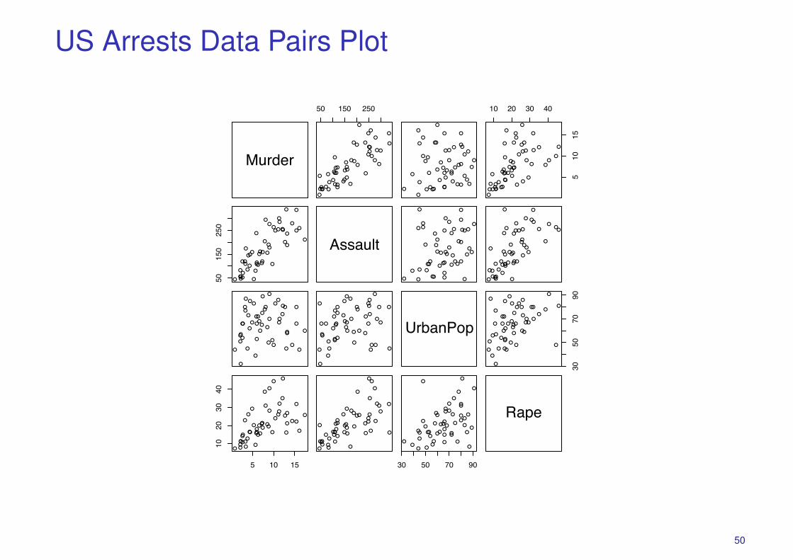
US Arrests Data Pairs Plot
Murder
50 150 250
●
●
●● ●●
●
●
●
●
●
●
●
●
●
●
●
●
●
●
●
●
●
●
●
●
●
●
●
●
●●
●
●
●●
●
●
●
●
●
●●
●●
●
●
●
●
●
●
●
●● ●
●
●
●
●
●
●
●
●
●
●
●
●
●
●
●
●
●
●
●
●
●
●
●
●
●
● ●
●
●
●●
●
●
●
●
●
● ●
●●
●
●
●
●
●
10 20 30 40
510
15
●
●
●● ●
●
●
●
●
●
●
●
●
●
●
●
●
●
●
●
●
●
●
●
●
●
●
●
●
●
●●
●
●
●●
●
●
●
●
●
●●
●●
●
●
●
●
●
50150
250
●
●
●
●
●
●
●
●
●
●
●
●
●
●
●
● ●
●
●
●
●
●
●
●
●
●●
●
●
●
●
●
●
●
●
●●
●
●
●
●
●●
●
●
●●
●
●
●Assault
●
●
●
●
●
●
●
●
●
●
●
●
●
●
●
●●
●
●
●
●
●
●
●
●
● ●
●
●
●
●
●
●
●
●
●●
●
●
●
●
●●
●
●
●●
●
●
●
●
●
●
●
●
●
●
●
●
●
●
●
●
●
●
●●
●
●
●
●
●
●
●
●
●●
●
●
●
●
●
●
●
●
● ●
●
●
●
●
●●
●
●
●●
●
●
●
●
●
●
●
●
●●
●
●
●
●
●
●
●
●
●
●
●
●
●
●
●
●
●
●
●
●
●
●
●
●
●
●●
●
●●
●
●
●●
●
●●
●
●
●
●
●
●●
●
●
●
●
●●
●
●
●
●
●
●
●
●
●
●
●
●
●
●
●
●
●
●
●
●
●
●
●
●
●
●●
●
●●
●
●
●●
●
●●
●
●
●
●
●
● UrbanPop
3050
7090
●
●
●
●
●
●●
●
●
●
●
●
●
●
●
●
●
●
●
●
●
●
●
●
●
●
●
●
●
●
●
●
●●
●
● ●
●
●
●●
●
●●
●
●
●
●
●
●
5 10 15
1020
3040
●
●
●
●
●●
●
●
●
●
●
●
●●
●
●●
●
●
●
●
●
●●
●
●●
●
●
●
●
●
●
●
●●
●
●
●
●
●
●●
●
●
●
●
●●
●
●
●
●
●
●●
●
●
●
●
●
●
●●
●
●●
●
●
●
●
●
●●
●
●●
●
●
●
●
●
●
●
●●
●
●
●
●
●
●●
●
●
●
●
●●
●
30 50 70 90
●
●
●
●
●●
●
●
●
●
●
●
●●
●
●●
●
●
●
●
●
●●
●
● ●
●
●
●
●
●
●
●
●●
●
●
●
●
●
●●●
●
●
●
●●
●
Rape
50

US Arrests Data Biplot
−0.2 −0.1 0.0 0.1 0.2 0.3
−0.2
−0.1
0.0
0.1
0.2
0.3
Comp.1
Com
p.2
AlabamaAlaska
Arizona
Arkansas
California
ColoradoConnecticut
Delaware
Florida
Georgia
Hawaii
Idaho
Illinois
Indiana IowaKansas
KentuckyLouisiana
MaineMaryland
Massachusetts
Michigan
Minnesota
Mississippi
Missouri
Montana
Nebraska
Nevada
New Hampshire
New Jersey
New Mexico
New York
North Carolina
North Dakota
Ohio
Oklahoma
Oregon Pennsylvania
Rhode Island
South Carolina
South DakotaTennessee
Texas
Utah
Vermont
Virginia
Washington
West Virginia
Wisconsin
Wyoming
−5 0 5
−50
5
Murder
Assault
UrbanPop
Rape
51

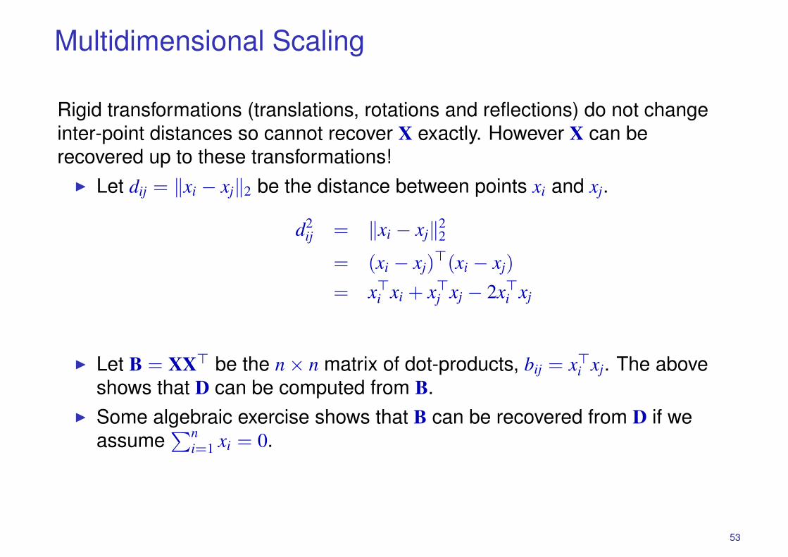
Multidimensional Scaling
Suppose there are n points X in Rp, but we are only given the n × n matrix D of
inter-point distances.
Can we reconstruct X?
52
Multidimensional Scaling
Rigid transformations (translations, rotations and reflections) do not changeinter-point distances so cannot recover X exactly. However X can berecovered up to these transformations!
� Let dij = �xi − xj�2 be the distance between points xi and xj.
d2ij = �xi − xj�
22
= (xi − xj)�(xi − xj)
= x�i xi + x�j xj − 2x�i xj
� Let B = XX� be the n × n matrix of dot-products, bij = x�i xj. The aboveshows that D can be computed from B.
� Some algebraic exercise shows that B can be recovered from D if weassume
�ni=1 xi = 0.
53
Multidimensional Scaling
� If we knew X, then SVD gives X = UDV�. As X has rank k = min(n, p),we have at most k singular values in D and we can assume U ∈ R
n×k,D ∈ R
k×p and V ∈ Rp×p.
� The eigendecomposition of B is then:
B = XX� = UDD�U� = UΛU�.
� This eigendecomposition can be obtained from B without knowledge of X!� Let x̃�i = UiΛ
12 be the ith row of UΛ
12 . Pad x̃i with 0s so that it has length p.
x̃�i x̃j = UiΛU�
j = bij = x�i xj
and we have found a set of vectors with dot-products given by B.� The vectors x̃i differs from xi only via the orthogonal matrix V so are
equivalent up to rotation and reflections.
54

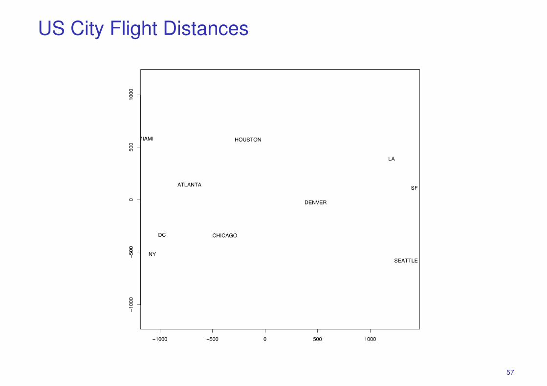
US City Flight Distances
We present a table of flying mileages between 10 American cities, distancescalculated from our 2-dimensional world. Using D as the starting point, metricMDS finds a configuration with the same distance matrix.
ATLA CHIG DENV HOUS LA MIAM NY SF SEAT DC0 587 1212 701 1936 604 748 2139 2182 543587 0 920 940 1745 1188 713 1858 1737 5971212 920 0 879 831 1726 1631 949 1021 1494701 940 879 0 1374 968 1420 1645 1891 12201936 1745 831 1374 0 2339 2451 347 959 2300604 1188 1726 968 2339 0 1092 2594 2734 923748 713 1631 1420 2451 1092 0 2571 2408 2052139 1858 949 1645 347 2594 2571 0 678 24422182 1737 1021 1891 959 2734 2408 678 0 2329543 597 1494 1220 2300 923 205 2442 2329 0
55
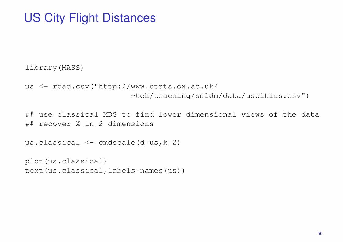
US City Flight Distances
library(MASS)
us <- read.csv("http://www.stats.ox.ac.uk/~teh/teaching/smldm/data/uscities.csv")
## use classical MDS to find lower dimensional views of the data## recover X in 2 dimensions
us.classical <- cmdscale(d=us,k=2)
plot(us.classical)text(us.classical,labels=names(us))
56
US City Flight Distances
−1000 −500 0 500 1000
−1000
−500
0500
1000
ATLANTA
CHICAGO
DENVER
HOUSTON
LA
MIAMI
NY
SF
SEATTLE
DC
57
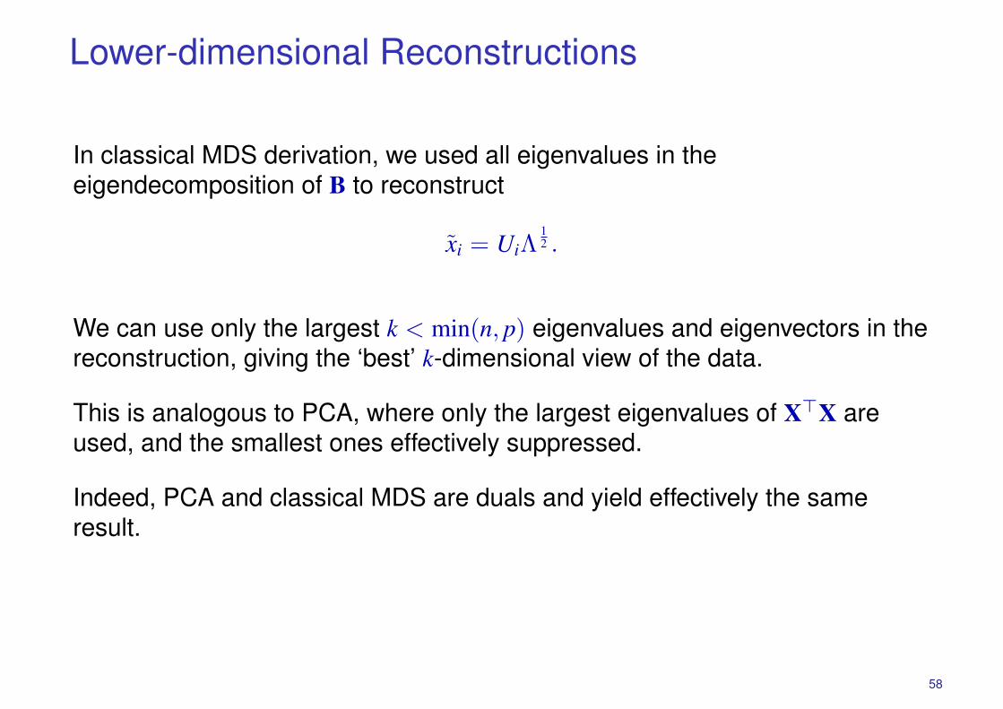
Lower-dimensional Reconstructions
In classical MDS derivation, we used all eigenvalues in theeigendecomposition of B to reconstruct
x̃i = UiΛ12 .
We can use only the largest k < min(n, p) eigenvalues and eigenvectors in thereconstruction, giving the ‘best’ k-dimensional view of the data.
This is analogous to PCA, where only the largest eigenvalues of X�X areused, and the smallest ones effectively suppressed.
Indeed, PCA and classical MDS are duals and yield effectively the sameresult.
58

Crabs Datalibrary(MASS)Crabs <- crabs[,4:8]Crabs.class <- factor(paste(crabs[,1],crabs[,2],sep=""))
crabsmds <- cmdscale(d= dist(Crabs),k=2)plot(crabsmds, pch=20, cex=2,col=unclass(Crabs.class))
●
●
●●●
●
●
●
●
●
●
●
●
●
●
●
●
●
●
●
●
●
●
●
●
●
●
●
●
●
●●
●●
●
● ●●● ●
●
●
●
●
●
●
●
●
●
●
● ●
●
●●
●●●
●
●
● ● ●
●
●
●
●●
●
●
●
●
●
●
●
●
●
●●
●
●
●●
●●
●
●●
●●
●
●
●
●●
●
●
●
●
●● ●
●
●
●
●
● ●
●
●●
●●
●●
● ●
●
● ●
●●
●
●
●
● ●
●
●
●●
●
●
●●
●
●
●
●
●
● ●
●
●●
●
●
●●
●
●
●●
●
●
●●
●
●
●
●
●
●
●
●
●●
● ●●
●
●
●
●
●
●
●●
●
●
●
●
●
●
● ●●
●
●
●
●
●
●
●
●
●
●●
●
●
−30 −20 −10 0 10 20
−3−2
−10
12
MDS 1
MD
S 2
59
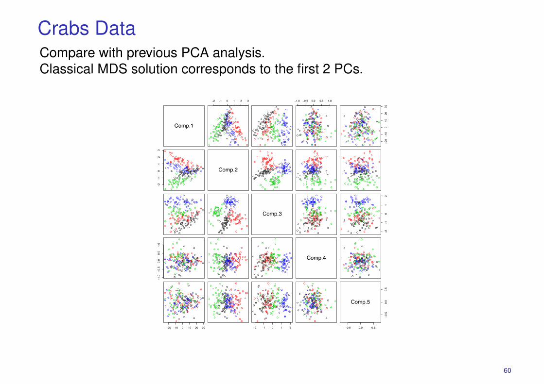
Crabs DataCompare with previous PCA analysis.Classical MDS solution corresponds to the first 2 PCs.
Comp.1
−2 −1 0 1 2 3 −1.0 −0.5 0.0 0.5 1.0
−20
−10
010
2030
−2−1
01
23
Comp.2
Comp.3
−2−1
01
2
−1.0
−0.5
0.0
0.5
1.0
Comp.4
−20 −10 0 10 20 30 −2 −1 0 1 2 −0.5 0.0 0.5
−0.5
0.0
0.5
Comp.5
60
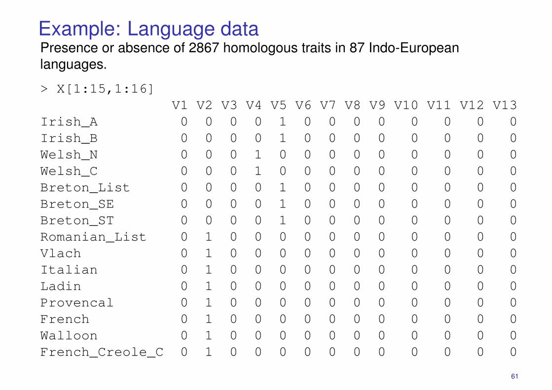
Example: Language dataPresence or absence of 2867 homologous traits in 87 Indo-Europeanlanguages.
> X[1:15,1:16]V1 V2 V3 V4 V5 V6 V7 V8 V9 V10 V11 V12 V13 V14 V15 V16
Irish_A 0 0 0 0 1 0 0 0 0 0 0 0 0 0 0 0Irish_B 0 0 0 0 1 0 0 0 0 0 0 0 0 0 0 0Welsh_N 0 0 0 1 0 0 0 0 0 0 0 0 0 0 0 0Welsh_C 0 0 0 1 0 0 0 0 0 0 0 0 0 0 0 0Breton_List 0 0 0 0 1 0 0 0 0 0 0 0 0 0 0 0Breton_SE 0 0 0 0 1 0 0 0 0 0 0 0 0 0 0 0Breton_ST 0 0 0 0 1 0 0 0 0 0 0 0 0 0 0 0Romanian_List 0 1 0 0 0 0 0 0 0 0 0 0 0 0 0 0Vlach 0 1 0 0 0 0 0 0 0 0 0 0 0 0 0 0Italian 0 1 0 0 0 0 0 0 0 0 0 0 0 0 0 0Ladin 0 1 0 0 0 0 0 0 0 0 0 0 0 0 0 0Provencal 0 1 0 0 0 0 0 0 0 0 0 0 0 0 0 0French 0 1 0 0 0 0 0 0 0 0 0 0 0 0 0 0Walloon 0 1 0 0 0 0 0 0 0 0 0 0 0 0 0 0French_Creole_C 0 1 0 0 0 0 0 0 0 0 0 0 0 0 0 0
61
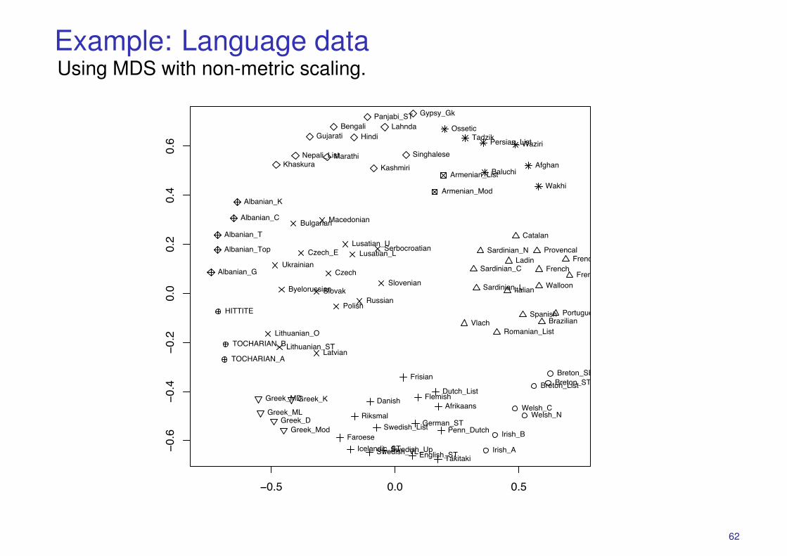
Example: Language dataUsing MDS with non-metric scaling.
MDS (i.e. cmdscale) which minimizes (d2ij − d̃2
ij)2. Sammon thereby puts
more weight on reproducing the separation of points which are close byforcing them apart. Projection by MDS(Jaccard/sammon) with cluster dis-covery by k-means (Jaccard): There is an obvious east to west (top-left to
!0.5 0.0 0.5
!0.6
!0.4
!0.2
0.0
0.2
0.4
0.6
Irish_A
Irish_B
Welsh_NWelsh_C
Breton_List
Breton_SE
Breton_ST
Romanian_ListVlach
Italian
Ladin
Provencal
French
Walloon
French_Creole_C
French_Creole_D
Sardinian_N
Sardinian_L
Sardinian_C
Spanish Portuguese_STBrazilian
Catalan
German_STPenn_Dutch
Dutch_List
Afrikaans
Flemish
Frisian
Swedish_UpSwedish_VL
Swedish_List
Danish
Riksmal
Icelandic_ST
Faroese
English_STTakitaki
Lithuanian_O
Lithuanian_STLatvian
Slovenian
Lusatian_L
Lusatian_U
Czech
Slovak
Czech_E
Ukrainian
Byelorussian
PolishRussian
MacedonianBulgarian
Serbocroatian
Gypsy_Gk
Singhalese
Kashmiri
Marathi
Gujarati
Panjabi_ST
Lahnda
Hindi
Bengali
Nepali_List
Khaskura
Greek_ML
Greek_MD
Greek_Mod
Greek_D
Greek_K
Armenian_Mod
Armenian_List
Ossetic
Afghan
WaziriPersian_ListTadzik
Baluchi
Wakhi
Albanian_T
Albanian_Top
Albanian_G
Albanian_K
Albanian_C
HITTITE
TOCHARIAN_A
TOCHARIAN_B
bottom-right) separation of languages in the MDS and the clusters in theMDS grouping agree with the clusters discovered by agglomerative clus-tering and k-means. The two clustering methods group languages slightlydifferently with k-means splitting the Germanic languages.
## (alternative/MDS) make a field to display the clusters## use MDS - sammon does this nicelydi.sam <- sammon(D,magic=0.20000002,niter=1000,tol=1e-8)eqscplot(di.sam$points,pch=km$cluster,col=km$cluster)text(di.sam$points,labels=row.names(X),pos=4,col=km$cluster)
5
62
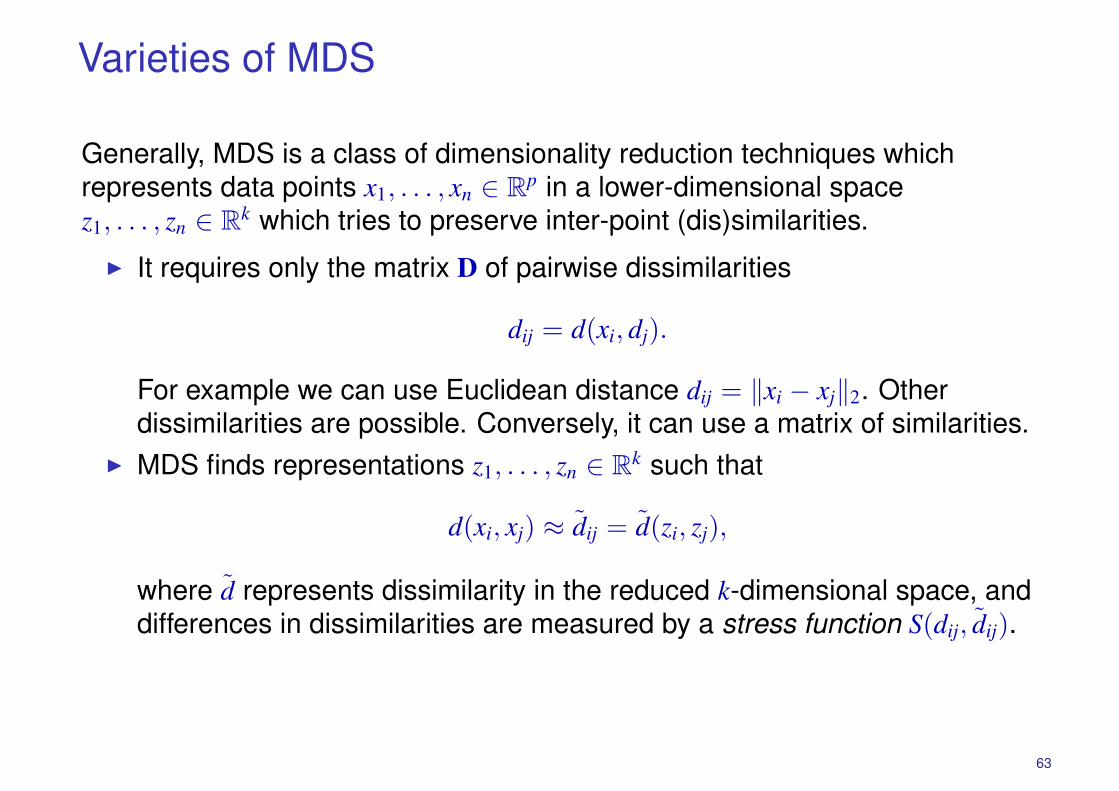
Varieties of MDS
Generally, MDS is a class of dimensionality reduction techniques whichrepresents data points x1, . . . , xn ∈ R
p in a lower-dimensional spacez1, . . . , zn ∈ R
k which tries to preserve inter-point (dis)similarities.� It requires only the matrix D of pairwise dissimilarities
dij = d(xi, dj).
For example we can use Euclidean distance dij = �xi − xj�2. Otherdissimilarities are possible. Conversely, it can use a matrix of similarities.
� MDS finds representations z1, . . . , zn ∈ Rk such that
d(xi, xj) ≈ d̃ij = d̃(zi, zj),
where d̃ represents dissimilarity in the reduced k-dimensional space, anddifferences in dissimilarities are measured by a stress function S(dij, d̃ij).
63
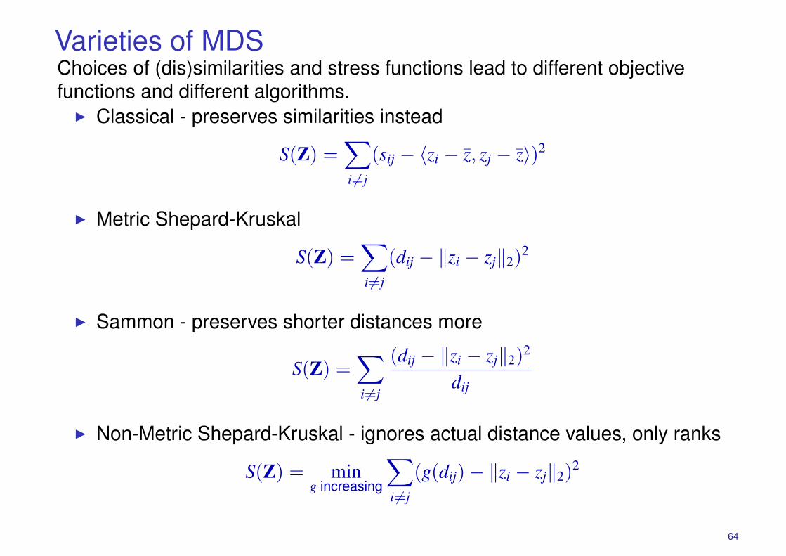
Varieties of MDSChoices of (dis)similarities and stress functions lead to different objectivefunctions and different algorithms.
� Classical - preserves similarities instead
S(Z) =�
i�=j
(sij − �zi − z̄, zj − z̄�)2
� Metric Shepard-Kruskal
S(Z) =�
i�=j
(dij − �zi − zj�2)2
� Sammon - preserves shorter distances more
S(Z) =�
i �=j
(dij − �zi − zj�2)2
dij
� Non-Metric Shepard-Kruskal - ignores actual distance values, only ranks
S(Z) = ming increasing
�
i �=j
(g(dij)− �zi − zj�2)2
64
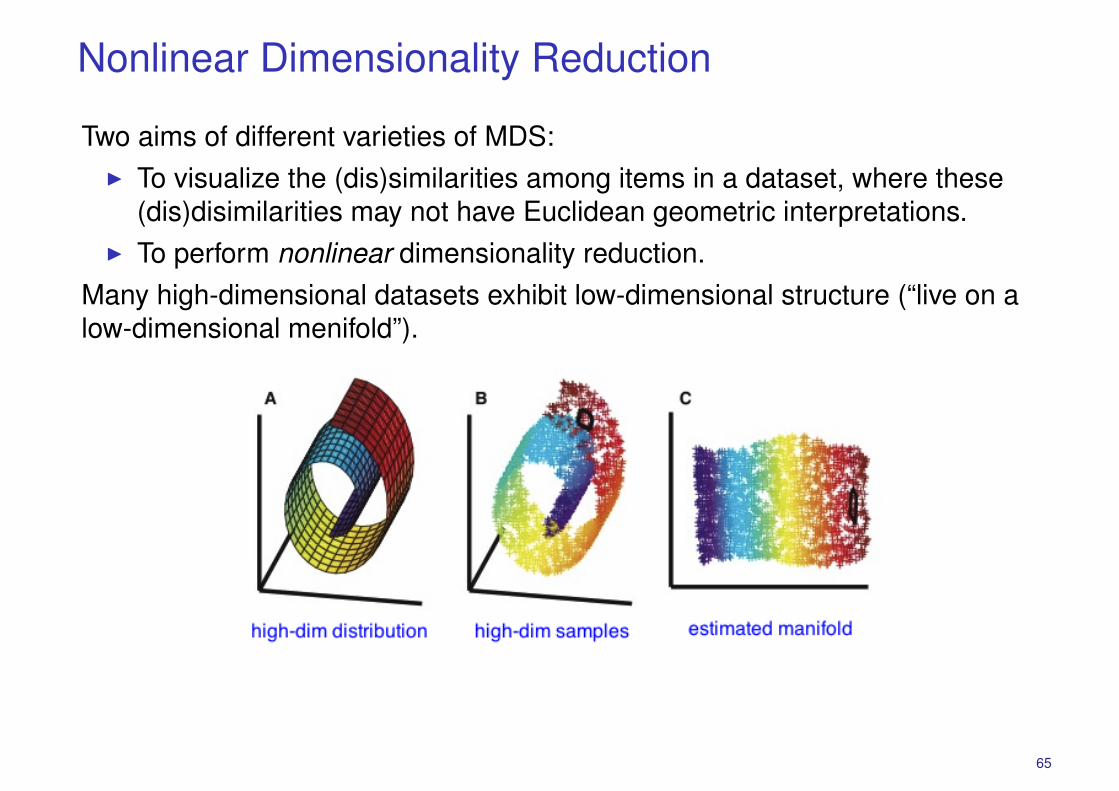
Nonlinear Dimensionality Reduction
Two aims of different varieties of MDS:� To visualize the (dis)similarities among items in a dataset, where these
(dis)disimilarities may not have Euclidean geometric interpretations.� To perform nonlinear dimensionality reduction.
Many high-dimensional datasets exhibit low-dimensional structure (“live on alow-dimensional menifold”).
65
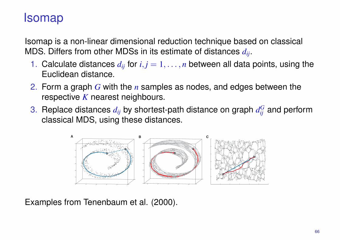
Isomap
Isomap is a non-linear dimensional reduction technique based on classicalMDS. Differs from other MDSs in its estimate of distances dij.
1. Calculate distances dij for i, j = 1, . . . , n between all data points, using theEuclidean distance.
2. Form a graph G with the n samples as nodes, and edges between therespective K nearest neighbours.
3. Replace distances dij by shortest-path distance on graph dGij and perform
classical MDS, using these distances.
converts distances to inner products (17 ),which uniquely characterize the geometry ofthe data in a form that supports efficientoptimization. The global minimum of Eq. 1 isachieved by setting the coordinates yi to thetop d eigenvectors of the matrix !(DG) (13).
As with PCA or MDS, the true dimen-sionality of the data can be estimated fromthe decrease in error as the dimensionality ofY is increased. For the Swiss roll, whereclassical methods fail, the residual varianceof Isomap correctly bottoms out at d " 2(Fig. 2B).
Just as PCA and MDS are guaranteed,given sufficient data, to recover the truestructure of linear manifolds, Isomap is guar-anteed asymptotically to recover the true di-mensionality and geometric structure of astrictly larger class of nonlinear manifolds.Like the Swiss roll, these are manifolds
whose intrinsic geometry is that of a convexregion of Euclidean space, but whose ambi-ent geometry in the high-dimensional inputspace may be highly folded, twisted, orcurved. For non-Euclidean manifolds, such asa hemisphere or the surface of a doughnut,Isomap still produces a globally optimal low-dimensional Euclidean representation, asmeasured by Eq. 1.
These guarantees of asymptotic conver-gence rest on a proof that as the number ofdata points increases, the graph distancesdG(i, j) provide increasingly better approxi-mations to the intrinsic geodesic distancesdM(i, j), becoming arbitrarily accurate in thelimit of infinite data (18, 19). How quicklydG(i, j) converges to dM(i, j) depends on cer-tain parameters of the manifold as it lieswithin the high-dimensional space (radius ofcurvature and branch separation) and on the
density of points. To the extent that a data setpresents extreme values of these parametersor deviates from a uniform density, asymp-totic convergence still holds in general, butthe sample size required to estimate geodes-ic distance accurately may be impracticallylarge.
Isomap’s global coordinates provide asimple way to analyze and manipulate high-dimensional observations in terms of theirintrinsic nonlinear degrees of freedom. For aset of synthetic face images, known to havethree degrees of freedom, Isomap correctlydetects the dimensionality (Fig. 2A) and sep-arates out the true underlying factors (Fig.1A). The algorithm also recovers the knownlow-dimensional structure of a set of noisyreal images, generated by a human hand vary-ing in finger extension and wrist rotation(Fig. 2C) (20). Given a more complex dataset of handwritten digits, which does not havea clear manifold geometry, Isomap still findsglobally meaningful coordinates (Fig. 1B)and nonlinear structure that PCA or MDS donot detect (Fig. 2D). For all three data sets,the natural appearance of linear interpolationsbetween distant points in the low-dimension-al coordinate space confirms that Isomap hascaptured the data’s perceptually relevantstructure (Fig. 4).
Previous attempts to extend PCA andMDS to nonlinear data sets fall into twobroad classes, each of which suffers fromlimitations overcome by our approach. Locallinear techniques (21–23) are not designed torepresent the global structure of a data setwithin a single coordinate system, as we do inFig. 1. Nonlinear techniques based on greedyoptimization procedures (24–30) attempt todiscover global structure, but lack the crucialalgorithmic features that Isomap inheritsfrom PCA and MDS: a noniterative, polyno-mial time procedure with a guarantee of glob-al optimality; for intrinsically Euclidean man-
Fig. 2. The residualvariance of PCA (opentriangles), MDS [opentriangles in (A) through(C); open circles in (D)],and Isomap (filled cir-cles) on four data sets(42). (A) Face imagesvarying in pose and il-lumination (Fig. 1A).(B) Swiss roll data (Fig.3). (C) Hand imagesvarying in finger exten-sion and wrist rotation(20). (D) Handwritten“2”s (Fig. 1B). In all cas-es, residual variance de-creases as the dimen-sionality d is increased.The intrinsic dimen-sionality of the datacan be estimated bylooking for the “elbow”at which this curve ceases to decrease significantly with added dimensions. Arrows mark the true orapproximate dimensionality, when known. Note the tendency of PCA and MDS to overestimate thedimensionality, in contrast to Isomap.
Fig. 3. The “Swiss roll” data set, illustrating how Isomap exploits geodesicpaths for nonlinear dimensionality reduction. (A) For two arbitrary points(circled) on a nonlinear manifold, their Euclidean distance in the high-dimensional input space (length of dashed line) may not accuratelyreflect their intrinsic similarity, as measured by geodesic distance alongthe low-dimensional manifold (length of solid curve). (B) The neighbor-hood graph G constructed in step one of Isomap (with K " 7 and N "
1000 data points) allows an approximation (red segments) to the truegeodesic path to be computed efficiently in step two, as the shortestpath in G. (C) The two-dimensional embedding recovered by Isomap instep three, which best preserves the shortest path distances in theneighborhood graph (overlaid). Straight lines in the embedding (blue)now represent simpler and cleaner approximations to the true geodesicpaths than do the corresponding graph paths (red).
R E P O R T S
www.sciencemag.org SCIENCE VOL 290 22 DECEMBER 2000 2321
on D
ecem
ber
5, 2008
ww
w.s
cie
ncem
ag.o
rgD
ow
nlo
aded fro
m
Examples from Tenenbaum et al. (2000).
66

Handwritten Characters
tion to geodesic distance. For faraway points,geodesic distance can be approximated byadding up a sequence of “short hops” be-tween neighboring points. These approxima-tions are computed efficiently by findingshortest paths in a graph with edges connect-ing neighboring data points.
The complete isometric feature mapping,or Isomap, algorithm has three steps, whichare detailed in Table 1. The first step deter-mines which points are neighbors on themanifold M, based on the distances dX (i, j)between pairs of points i, j in the input space
X. Two simple methods are to connect eachpoint to all points within some fixed radius !,or to all of its K nearest neighbors (15). Theseneighborhood relations are represented as aweighted graph G over the data points, withedges of weight dX(i, j) between neighboringpoints (Fig. 3B).
In its second step, Isomap estimates thegeodesic distances dM (i, j) between all pairsof points on the manifold M by computingtheir shortest path distances dG(i, j) in thegraph G. One simple algorithm (16 ) for find-ing shortest paths is given in Table 1.
The final step applies classical MDS tothe matrix of graph distances DG " {dG(i, j)},constructing an embedding of the data in ad-dimensional Euclidean space Y that bestpreserves the manifold’s estimated intrinsicgeometry (Fig. 3C). The coordinate vectors yi
for points in Y are chosen to minimize thecost function
E ! !#$DG% " #$DY%!L2 (1)
where DY denotes the matrix of Euclideandistances {dY(i, j) " !yi & yj!} and !A!L2
the L2 matrix norm '(i, j Ai j2 . The # operator
Fig. 1. (A) A canonical dimensionality reductionproblem from visual perception. The input consistsof a sequence of 4096-dimensional vectors, rep-resenting the brightness values of 64 pixel by 64pixel images of a face rendered with differentposes and lighting directions. Applied to N " 698raw images, Isomap (K" 6) learns a three-dimen-sional embedding of the data’s intrinsic geometricstructure. A two-dimensional projection is shown,with a sample of the original input images (redcircles) superimposed on all the data points (blue)and horizontal sliders (under the images) repre-senting the third dimension. Each coordinate axisof the embedding correlates highly with one de-gree of freedom underlying the original data: left-right pose (x axis, R " 0.99), up-down pose ( yaxis, R " 0.90), and lighting direction (slider posi-tion, R " 0.92). The input-space distances dX(i, j )given to Isomap were Euclidean distances be-tween the 4096-dimensional image vectors. (B)Isomap applied to N " 1000 handwritten “2”sfrom the MNIST database (40). The two mostsignificant dimensions in the Isomap embedding,shown here, articulate the major features of the“2”: bottom loop (x axis) and top arch ( y axis).Input-space distances dX(i, j ) were measured bytangent distance, a metric designed to capture theinvariances relevant in handwriting recognition(41). Here we used !-Isomap (with ! " 4.2) be-cause we did not expect a constant dimensionalityto hold over the whole data set; consistent withthis, Isomap finds several tendrils projecting fromthe higher dimensional mass of data and repre-senting successive exaggerations of an extrastroke or ornament in the digit.
R E P O R T S
22 DECEMBER 2000 VOL 290 SCIENCE www.sciencemag.org2320
on D
ecem
ber
5, 2008
ww
w.s
cie
ncem
ag.o
rgD
ow
nlo
aded fro
m
67

Faces
tion to geodesic distance. For faraway points,geodesic distance can be approximated byadding up a sequence of “short hops” be-tween neighboring points. These approxima-tions are computed efficiently by findingshortest paths in a graph with edges connect-ing neighboring data points.
The complete isometric feature mapping,or Isomap, algorithm has three steps, whichare detailed in Table 1. The first step deter-mines which points are neighbors on themanifold M, based on the distances dX (i, j)between pairs of points i, j in the input space
X. Two simple methods are to connect eachpoint to all points within some fixed radius !,or to all of its K nearest neighbors (15). Theseneighborhood relations are represented as aweighted graph G over the data points, withedges of weight dX(i, j) between neighboringpoints (Fig. 3B).
In its second step, Isomap estimates thegeodesic distances dM (i, j) between all pairsof points on the manifold M by computingtheir shortest path distances dG(i, j) in thegraph G. One simple algorithm (16 ) for find-ing shortest paths is given in Table 1.
The final step applies classical MDS tothe matrix of graph distances DG " {dG(i, j)},constructing an embedding of the data in ad-dimensional Euclidean space Y that bestpreserves the manifold’s estimated intrinsicgeometry (Fig. 3C). The coordinate vectors yi
for points in Y are chosen to minimize thecost function
E ! !#$DG% " #$DY%!L2 (1)
where DY denotes the matrix of Euclideandistances {dY(i, j) " !yi & yj!} and !A!L2
the L2 matrix norm '(i, j Ai j2 . The # operator
Fig. 1. (A) A canonical dimensionality reductionproblem from visual perception. The input consistsof a sequence of 4096-dimensional vectors, rep-resenting the brightness values of 64 pixel by 64pixel images of a face rendered with differentposes and lighting directions. Applied to N " 698raw images, Isomap (K" 6) learns a three-dimen-sional embedding of the data’s intrinsic geometricstructure. A two-dimensional projection is shown,with a sample of the original input images (redcircles) superimposed on all the data points (blue)and horizontal sliders (under the images) repre-senting the third dimension. Each coordinate axisof the embedding correlates highly with one de-gree of freedom underlying the original data: left-right pose (x axis, R " 0.99), up-down pose ( yaxis, R " 0.90), and lighting direction (slider posi-tion, R " 0.92). The input-space distances dX(i, j )given to Isomap were Euclidean distances be-tween the 4096-dimensional image vectors. (B)Isomap applied to N " 1000 handwritten “2”sfrom the MNIST database (40). The two mostsignificant dimensions in the Isomap embedding,shown here, articulate the major features of the“2”: bottom loop (x axis) and top arch ( y axis).Input-space distances dX(i, j ) were measured bytangent distance, a metric designed to capture theinvariances relevant in handwriting recognition(41). Here we used !-Isomap (with ! " 4.2) be-cause we did not expect a constant dimensionalityto hold over the whole data set; consistent withthis, Isomap finds several tendrils projecting fromthe higher dimensional mass of data and repre-senting successive exaggerations of an extrastroke or ornament in the digit.
R E P O R T S
22 DECEMBER 2000 VOL 290 SCIENCE www.sciencemag.org2320
on
De
ce
mb
er
5,
20
08
w
ww
.scie
nce
ma
g.o
rgD
ow
nlo
ad
ed
fro
m
68
Other Nonlinear Dimensionality Reduction Techniques
� Locally Linear Embedding.� Laplacian Eigenmaps.� Maximum Variance Unfolding.
69