msa brief outline of ... detailed flowfield predictions for several three-dimensional nozzle con-...
TRANSCRIPT

NASA Contractor Report’ 3%4
Numerical Method for Predicting Flow Characteristics and Performance of .Nonaxisymmetric Nozzles
Part 2 - Applications
P. D. Thomas
CONTRACT NAS 1-l 5084 OCTOBER 1980
MSA
https://ntrs.nasa.gov/search.jsp?R=19800024846 2018-06-23T03:22:43+00:00Z

NASA Contractor Report 3264
Numerical Method for Predicting Flow Characteristics and Performance of Nonaxisymmetric Nozzles
Part 2 - Applications
P. D. Thomas
Lockheed Missiles and Space Conzpauy, Im. Palo Alto, California
Prepared for Langley Research Center under Contract NASl-15084
National Aeronautics and Space Administration
Scientific and Technical Information Branch
1980

---- -.. .-

CONTENTS
Section -__ Page
1 INTRODUCTION ................................................. 1
2 MODIFICATIONS TO THE NUMERICAL METHOD ........................ 3
2.1 Brief Outline of the Original Formulation ............... 3
2.2 Modified Formulation of the Implicit Algorithm .......... 7
2.3 Modified Scheme for Subsonic Inflow and Outflow Boundary Conditions ..................................... 12
2.3.1 Inflow Boundary Points ........................... 12
2.3.2 Outflow Boundary Points .......................... I2
2.4 Implicit Dissipation .................................... I3
2.5 Improved Numerical Grid Generation Technique ............ I6
3 EVALUATION OF NOZZLE THRUST AND DISCHARGE COEFFICIENT ........ 23
3.1 Thrust .................................................. 23
3.2 Discharge Coefficient ................................... 27
4 FINAL FORMULATION OF TURBULENCE MODELS ....................... 29
4.1 Two-Dimensional and Axisymmetric Flows .................. 30
4.1.1 Wall Boundary Layers ............................. 32
4.1.2 Wakes ............................................ 36
4.1.3 Mixing Layers and Fully-Developed Jet Region ..... 38
4.2 General Three-Dimensional Flows ......................... 40
5 NUMERICAL EXPERIMENTS ........................................ 43
5.1
5.2
5.3
5.4
5.5
Computation of Separated Flow . . . . . . . . . . . . . . . . . . . . . . . . . . . 43
Effect of Implicit Boundary Conditions and Time Stepsize on the Solution . . . . . . . . . . . . . . . . . . . . . . . . . . . . . . . . 51
5.2.1 Implicit Boundary Conditions . . . . . . . . . . . . . . . . . . . . . 51
5.2.2 Time Stepsize . . . . . . . . . . . . . . . . . . . . . . . . . . . . . . . . . . . . 53
Effect of Artificial Explicit Smoothing on the Solution . . 62
Effect of Artificial Implicit Dissipation on Stability and Convergence . . . . . . . . . . . . . . . . . . . . . . . . . . . . . . . . 64
Conclusions . . . . . . . . . . . . . . . . . . . . . . . . . . . . . . . . . . . . . . . . . . . . . . 71
iii

Section Page
6 NOZZLE FLOWFIELD PREDICTIONS AND COMPARISON WITH EXPERIMENTAL DATA ,..,.~..,...,.,,........................... 73
6.1 Internal Flow in a "Two-Dimensional" Converging- Diverging Nozzle ,.................................-.... 73
6.1.1 Configuration, Operating Conditions, and Computational Grid . . . . . . . . . . . . . . . . . . . . . . . . . . . . . . 73
6.1.2 Two-Dimensional Flow Results . . . . . . . . . . . . . . . . . . . . . 79
6.1.3 Three-Dimensional Flow Results . . . . . . . . . . . . . . . . . . . 91
6.2 Internal and External Flowfield of a Circular Nozzle . . . . 98
6.2.1 Configuration, Operating Conditions, and Computational Grid . . . . . . . . . . . . . . . . . . . . . . . . . . . . . . . 98
6.2.2 Numerical Results . . . . . . . . . . . . . . . . . . . . . . . . . . . . . ...104
7 REFERENCES . . . . . . . . . . . . . . . . . . . . . . . . . . . . . . . . . . . . . . . . . . . . . . . . ...113
iv

Section 1
INTRODUCTION
This report summarizes work performed during the second phase of an effort to
develop a computer-implemented numerical method for predicting the flow charac-
teristics and performance of three-dimensional jet engine exhaust nozzles. The
objective of developing a method for computing the internal and external viscous
flowfield of an isolated nozzle has been met. The approach is based on using
an implicit numerical method to solve the unsteady Navier-Stokes equations in
a boundary-conforming curvilinear coordinate system to obtain the desired time-
asymptotic steady state solution. Flow turbulence effects are simulated by
means of algebraic turbulence models for the effective turbulent eddy viscosity
and Prandtl number. A detailed description of the equations and boundary con-
ditions and of the numerical method have been presented in an earlier report
[Ref. 11, along with a general discussion of turbulence models appropriate to
the various sub-regions of the nozzle flowfield.
The present final report describes work performed since Reference 1 was written.
Recent modifications and improvements to the original numerical algorithm are
presented in Section 2. Section 3 gives the equations that are used to derive
the nozzle performance parameters such as thrust and discharge coefficient
from the computed flowfield data. The final formulation of the turbulence
models that are used to simulate flow turbulence effects is presented in
Section 4. Section 5 presents the results of numerical experiments performed
to explore the effect that various parameters in the numerical method have on
both the rate of convergence to steady state and on the final flowfield solu-
tion. Detailed flowfield predictions for several three-dimensional nozzle con-
figurations are presented in Section 6 and compared with experimental wind
tunnel data.
The numerical method is embodied in a set of three computer codes: RGRIDD,
NOZLIC, and NOZL3D. The RGRIDD code constructs the curvilinear coordinate

system and computational grid numerically for nozzles of complex geometric
configuration. The NOZLIC code generates a set of flowfield initial condi-
tions on this grid that are used to start a flow computation. The NOZL3D
code performs the actual flowfield computation and evaluates the nozzle per-
formance characteristics. A user's guide to the operation of these three
codes is contained in a separate volume [Ref. 81.
In the sections that follow, all equations are cast in dimensionless form.
Distances are referred to a reference length, velocities are referred to the
speed of sound at some reference state, viscosity 1-1 is referred to the
molecular viscosity at the reference state, and individual state variables
such as density p, pressure p, and temperature T are referred to their
values at the reference state. The reference state is that at which the
Reynolds number Re is defined in terms of the reference length using the
reference sound speed as the characteristic velocity.

Section 2
MODIFICATIONS TO THE NUMERICAL METHOD
2.1 BRIEF OUTLINE OF THE ORIGINAL FORMULATION
The original formulation of the numerical method [Ref. 1] starts with the
strong conservation-law form of unsteady Navier-Stokes equations in a Cartesian
base coordinate system (xy z). The equations are transformed to a boundary-
conforming curvilinear coordinate system (s,n,<), and take the non-dimensional
form
iq + it; + ijn + i+i 5
= Re-'(^en + ir; ) (2.1)
where ;I = J; (2.2)
J is the Jacobian of the inverse transformation
J = a(x,y,z)/a(~,n,c) (2.3)
q is a vector of conserved variables whose components are the density, the
three Cartesian components of the momentum flux vector p;, and the total
energy per unit volume, i, g, and h are inviscid flux vectors; and the terms
on the R.H.S. of Eq. (2.1) that are inversely proportional to the Reynolds
number Re represent viscous transport processes. Each of the inviscid flux
vectors is a linear combination of the flux vectors ?, 6, 6 associated with
the Cartesian coordinate direction x, y, z, respectively. The coefficients
of these linear combinations are the metrics of the coordinate transformations
E(x*Y,z,t) 3 n(x,Y,z,t) 3 s(x,y,z,t). For example,
ix = J E, = Y, zs - y< zn
iy = J sy = z,~ xc - zs x0
etc. 3

The non-dimensional flow variable vector 5 and the inviscid flux vectors + -t -f f, g, h are defined as follows in terms of the Cartesian components u, v, w,
the density p, the pressure p, and the total energy per unit volume E:
5 = (P, PU, PV, PW, SIT
; = [pu, p'+ PU2, puv, puw, u(p' + e)lT
; = [pv, pvu, p’+ PV2, PVW¶ v(p' + EHT -+ h = [pw, pwu, PWV, P’+ PW2, W(P’ + E)lT
where p' = p/v and y is the specific heat ratio.
Similarly, each of the viscous terms i, i is a linear combination of the
viscous terms associated with each of the Cartesian coordinate directions. The
reader is referred to Section 2 of Reference 1 for the mathematical equations
that define the viscous terms. We note only that Eq. (2.1) represents the
parabolic approximation to the Navier-Stokes equations wherein viscous terms
associated with the streamise coordinate 5 are neglected.
To solve Equation (2.1), the transformed space (e. n, K) is covered by a
uniform grid (sj, nk, i;,) such that peripheral grid points lie on the bound-
aries of the space. The spatially differenced form of the equations is derived
to second order accuracy in the mesh spacings AE, An, A5 by means of the
Finite-Volume Method. To each interior grid point of the transformed space
there corresponds a cell of volume AV = AC ATI A5 that encloses the point.
The difference equations that apply at the point are derived by integrating
Eq. (2.1) over the cell volume. This leads to difference equations of the form
(2.4a)
AV = A< Aq As (2.4b)

where the viscous terms have been suppressed for brevity, and where n. 6. J J
is the centered spatial differential operator for the cj direction
~j "j ~ = (fj+l k R - 'j-1 k ,)/2 , , , 3 (2.5)
and the central difference operators for the k and R directions are defined
similarly.
Within the second order spatial accuracy of the remaining terms, the volume
integral that appears in the first term of Eq. (2.4) may be represented in
terms of the cell-averaged value
6jk!z = (*v)-'
s ;r ck dn ds
Av (2.6)
which is centered at the grid point jka itself since the grid point is located
at the centroid of the cell that surrounds the point.
The final implicit space-time difference equations that govern the change An+1 A;I = q _ ;I" over a time Step AT = T n+l _ =n are obtained by evaluating
the spatially differentiated terms at the advanced time T n+l
, performing a
first-order Taylor series expansion about the solution at time -cn, and
factoring the implicit operator. This yields the implicit AD1 sequence
(I + AT pj 6j i)” Aq -**--[pj “j T + pk cTk i + j.19, Isk ii,” AT +... (2.7a)
A (I + AT u’k “k G +... )” A;l* = A{** (2.7b) -
,. A --* (I + AT pR 6& H + . . .)" Aq = Aq (2.7~)
,. . ,. where F, G, H are Jacobian matrices
(2.7d)
5
--.---- .~-
‘., .‘,

and where the viscous terms again have been suppressed for brevity. Each step
of the ADI sequence in Eq. (2.7) involves solving a block-tridiagonal linear
system of equations to obtain the solution at interior grid points.
For grid points located on the boundaries of the computational space s,n,s,
one or more of the five scalar components of Eq. (2.1) are replaced by algebraic
boundary conditions. If the latter are nonlinear in time, they are linearized
by a first-order Taylor series expansion about the solution 5". This yields a
linear algebraic subsystem of the form
M” ;1 = Tt;” (2.8)
The remaining scalar components of Eq. (2.1) (i.e., those scalar flow equations
that have not been replaced by the aforementioned algebraic boundary conditions)
are differenced by applying the finite-volume method in the same way as des-
cribed above for interior points. However, to a typical boundary point such
as j=l, there corresponds not a full cell, but rather a half-cell whose
width in the coordinate direction normal to the boundary is only half the width
A< of an interior cell. The counterpart of Equations (2.4) take the form
d ?I7 J
h ;I de dn d< + Aj F + uk 6k g + p'9. A, { = -. * , j = 1 (2.9a)
AV
AV = (Ac/2) An A< (2.9b)
where A. J
is the forward difference operator such that A. = fj+, - f.. The J J
volume integral in the first term of Eq. (2.9a) still may be represented in
terms of the value 4, at the cell centroid
;I, = (Av)-’ /
;I dc. dn ds (2.10)
Av
but the centroid is not located at the boundary grid point j = 1. However,
within-the spatial order of accuracy of Eq. (2.9), the value 4, may be
6
_.. _ -- __ ._ .____- --- ____-___ --- -
: :’ :_ . . .

evaluated by linear interpolation between the boundary point j = 1 and the
adjacent interior point j = 2.
;1* = (I +gAj) ;I * j=l (2.11)
where I is the identity operator.
. Equation (2.9a) is time-differenced implicitly and linearized in the same way
as is Eq. (2.4) for interior points. The appropriate scalar components of the
resulting equation are replaced by the linearized algebraic boundary conditions
(2.8) and the implicit operator is factored to obtain the counterpart of the
sequence (2.7) that applies at boundary points.
2.2 MODIFIED FORMULATION OF THE IMPLICIT ALGORITHM
The original formulation of the algorithm as presented in Reference 1 and
summarized in the preceding subsection has two deficiencies: (1) the algorithm
is valid only if the curvilinear coordinate transformation has no singular
points where the Jacobian J vanishes, and (2) unacceptably large truncation
errors can arise at grid points situated along the lines of intersection be-
tween boundary surfaces of the computational domain.
As an example where a singular transformation arises, consider the internal _
flow in an axisymmetric nozzle whose axis of symmetry coincides with the
Cartesian x axis, and whose interior wall is of radius r = r-w(x),
O<X<L. - - The first quadrant of the flow region interior to the nozzle can
be mapped onto a rectangular parallelepiped in a right-handed curvilinear
coordinate system 5, n, r by the transformation
5 = s(x), OlXlL
11 = -e , 0 ( cl 2 s/2
3 = 3(r) , 0 2 r 2 rw(x)
(2.12)
__ .-_ ..-^~_---- v-----r- T---~----i;*.< -__I- --
I ‘: . ., ,,,’ : ,, :,i : :‘- ,,, ‘,, : ,,.
., ‘. I_...~_ -1 ,,

where 8 = tan" y/z
r= \ly2+
One can verify easily that the Jacobian J of this transformation vanishes
at the axis of symmetry y = z = 0. The axis of symmetry maps onto the face
3 = 0 of the parallelepiped in the transformed space 5, n, 3; hence, the
transformation is singular at each point of that face.
The numerical mapping technique presented in Section 3 of Reference 1 also can
generate curvilinear coordinate systems that have isolated singularities. For
example, the quasi-elliptical mapping depicted in Figs. 3-3 and 3-4 of
Reference 1 has a singularity at the point A that corresponds to the focus
of the ellipse. The quasi-rectangular mapping given in Fig. 3-6 of Ref. 1
for the flow regions interior and exterior to a nozzle whose cross-section is
super-elliptical also has singularities at the points of maximum curvature of
the internal and external super-ellipses.
The numerical algorithm can be modified to handle isolated singularities such
as those in the foregoing examples. Two modifications are necessary: first,
as dictated by the finite-volume method, the Jacobian J at any grid point that
coincides with a coordinate singularity must be computed as a cell-averaged
quantity; and, second, the AD1 sequence (2.7) must be modified to yield a?j
directly, rather than A:, which involves the Jacobian as a factor. We shall
deal with these modifications in order.
In general, the flow variable vector ?$ is regular and non-zero even in the
neighborhood of a coordinate singularity, whereas the compound quantity { in
in Eq. (2.2) vanishes along with J at the singularity itself. Thus, Eq. (.2.6)
is a valid representation of the volume integral that appears in the first term
of Eq. (2.4a) only at grid points where the 5, n, 3 coordinate transformation
is non-singular. At a singular point, the quantity q vanishes locally,
whereas the volume integral is non-zero because it includes contributions from
all regular points within the finite-volume cell that encloses the singular
8

point. Since < itself is regular, the volume
evaluated by applying the mean value theorem
(Ad / ~ dg dn d3 = djk~ J*
AV. JkR
integral in Eq. (2.4a) can be
(2.13)
where the cell-averaged Jacobian J, is given by
J, = (AV)-’ J de dn dr; (2.14)
The latter is always non-zero for any cell of finite volume AV. If the singu-
larity coincides with an interior grid point, then the integral in Eq. (2.14)
can be evaluated analytically to second-order accuracy by introducing a local
Taylor series expansion for the function J( 5, n, 6). If the singularity
coincides with a boundary grid point, say j = 1, then the counterpart of
Eq. (2.13) is
(AV)-’ /
;; & dn dr; = 6, J* (2.15)
AV
where both ;* and J, represent cell-averaged values at the cell centroid,
and can be computed individually by linear interpolation between the boundary
point and the adjacent interior point (cf. Eq. (2.11)).
The alterations necessary to permit the direct computation of A;f from the
algorithm are merely a special case of the alterations that permit the use of
grids that move as a function of time (Ref. 2). One need only expand the term
4 as follows
A; = 6” AJ + Jntl A;
and redefine the Jacobian matrices in Eq. (2.7d) as

Upon factoring the implicit operator in the implicitly time-differenced and
linearized version of Eq. (2.4a), one obtains the AD1 sequence
(J
ntl 1 t AT ~j “j ~“)A~** = -6” AJ -(~j “j ” n 'k "k g (2.16a)
+pR 611 6) AT + . . .
(J n+l 1 + AT pk Ak iN + . ..) A;
* = Jn+l + *x
A4 (2.16b)
(J ‘+’ 1 -t AT pE 61? in + . . . ) A; = J n+l A$* (2.16~)
where AJ = 0 and J n+l = J” if the grid is stationary in time, i.e., if the
transformation (x,y,z)-t(c, n, r) is independent of time.
It is important to note that the form given in Eq. (2.8) must be retained when
applying algebraic boundary conditions at boundary grid points, or the values +**
of Aq and of A:* at boundary points will become inconsistent with those
at interior points where Eqs. (2.16) are employed. That is, for a stationary
grid, the boundary conditions must be written as
J M" A; = iii” (2.17)
The modified algorithm given in Eqs. (2.16) and (2.17) should be valid at grid
points that coincide with coordinate singularities as well as at regular points.
However, numerical experiments for axisymmetric flow yield poor numerical re-
sults for the flow variables at grid points situated along the singular axis
of symmetry, although the solution is accurate at all other points. We con-
jecture that the poor results at the symmetry axis result from a locally large
truncation error, inasmuch as care was taken to incorporate the symmetry pro-
perties of the flow variables and of the Cartesian coordinates into the computa-
tion of the metrics and of the explicit fourth order smoothing terms in the
10

* neighborhood of the axis. To obtain an accurate solution at points on the
axis, we have found it necessary to employ a time-lagging approach in which
the flow variables at axis points are extrapolated from those at adjacent
points following each time step. Even functions such as the temperature,
density, and axial velocity componentareextrapolated from those at the two
adjacent interior points using a second degree polynomial whose gradient is
zero at the axis, and odd functions such as the transverse velocity components
are set to zero at the axis.
Locally large truncation errors also are incurred at other types of coordinate
singularity, as well as exceptional but non-singular points of the curvilinear
coordinate system. Examples of the latter are grid points that lie along the
curves of intersection between two families of coordinate surface n = const.
and r = const. that represent nozzle wall boundaries, such as the interior or
exterior corner of a so-called "two-dimensional" nozzle that has flat walls
and a rectangular cross-section. Such a corner point has the characteristic
feature that the finite-volume cell associated with the point is either a
quarter-cell (interior corner) or a three-quarter-cell (exterior corner). To
avoid large numerical inaccuracies at such exceptional points, we have employed
a time-lagging approach similar to that outlined above for singular points of
an axisymmetric flow. For example, at axial corners where two walls intersect,
we merely interpolate the temperature and density from the nearest neighboring
wall points at 'the end of each time step.
* When the Cartesian x-axis coincides with the flowfield axis of synnnetry, the coordinates y, z and their associated velocity components, v, w are odd functions of position relative to the axis, whereas x and all
other flow variables are even functions.
11

2.3 MODIFIED SCHEME FOR SUBSONIC INFLOW AND OUTFLOW BOUNDARY CONDITIONS
2.3.1 Inflow Boundary Points
The scheme outlined in Section 4.2.2 of Reference 1 has been modified slightly
to avoid an obvious inconsistency at inflow boundary grid points that lie on
the nozzle walls. In the original inflow boundary scheme, four algebraic
boundary conditions are applied that specify the total pressure, the total
temperature, and the two direction cosines of the velocity vector. The fifth
relation that is required to close the system of equations governing the five
unknown components of the flow variable vector ;f is obtained from an implicit
finite-volume discretization of the mass conservation equation (the first
scalar component of Eq. (2.1)). This use of the mass conservation equation
to determine the density is invalid at wall points because it is inconsistent
with the density that is implied by the total pressure and total temperature
through the equation of state. This follows from the fact that total and
static temperatures are equal and total and static pressure are equal at wall
points where the velocity vanishes. Thus, the algebraic boundary conditions
alone are sufficient to determine the flow variables at wall points of the
inflow boundary. Note, however, that when the temperature Tw specified as
a boundary condition at nozzle walls, the inflow stagnation temperature boundary
condition must be equal to T, at points where the walls intersect the inflow
boundary.
2.3.2 Outflow Boundary Points
For cases where one is interested in computing only the flow internal to the
nozzle, the outflow boundary is positioned at the nozzle exit plane. When the
ambient pressure outside the nozzle is sufficiently high relative to the internal
flow stagnation chamber pressure, the flow will be wholly subsonic at the exit
plane, and the ambient pressure must be imposed as a boundary condition on the
static pressure at the outflow boundary IRef. 1, Section 2.4.61. In the original
implicit algorithm for outflow boundary grid points, this boundary condition is
linearized and used in place of the u-momentum equation. However, this results
12
in an inconsistent set of equations for the flow variables at grid points
located at the nozzle wall, where additional algebraic boundary conditions
on the velocity components and on either the wall temperature or heat flux
also are imposed. The inconsistency becomes apparent when one observes that,
for an adiabatic wall, the continuity and energy equations determine the gas
density and temperature at the wall. The corresponding wall pressure implied
by the equation of state in general will be inconsistent with the boundary
condition on the exit plane pressure. A similar inconsistency exists at wall
points when the wall temperature is specified as a boundary condition. The
inconsistency can be avoided by retaining the u-momentum equation at all out-
flow boundary points, and using the imposed exit pressure boundary condition
in place of the energy conservation equation. In addition, when the wall
temperature Tw is specified as a boundary condition, the algebraic equation
T = Tw is used in place of the continuity equation at wall points of the out-
flow boundary. The physical justification for this procedure is that the gas
density at the wall is determined completely by the exit pressure and wall
temperature boundary conditions alone.
2.4 IMPLICIT DISSIPATION
The implicit algorithm permits the use of large time steps AT without numeri-
cal instability, and makes it possible to attain the steady-state solution of
Eq. (2.1) in fewer time steps than would an explicit algorithm. However,
hundreds of time steps usually are required to achieve convergence to steady
state. In an effort to speed convergence, we have introduced artificial
dissipative terms into the implicit one-dimensional operators on the L.H.S.
of 'Eqs. (2.16). These dissipative terms are similar to those employed by
Steger [Ref. 31, except that they are differenced in a conservative fashion
and obey homogeneous boundary conditions. This ensures that the dissipative
terms do not alter the global conservation properties of the difference
equations [Ref. 1, Section 4.41.
The form of the dissipative term for the j coordinate direction is
13

, j=l
, l<j<j max
, ii = jmax
(2.18)
where u is a constant; E is the classical shift operator which is defined
such that for any mesh function f., E?m f = f
difference operator sjf = (Ei -
Jacobian in Eq. (2.3).
E;') :; j_+m ' 6 is the classical central
and J is the transformation
The central member of Eq. (2.18) applies at interior
points, and the first and last members apply at boundary points that are not
situated at flowfield symmetry planes. For such symmetry boundary points, the
dissipative terms are modified to account for the symmetry properties of G
and of J. With the addition of the dissipative term (2.18), the implicit
operator on the left side of Eq. (2.16a) for interior points assumes the form
(J n+l I + a “j J n+l
“j I ’ A~ ~j “j F”) A~ = . . .
Similar dissipative terms are added to the implicit operators in Eqs. (2.16b)
and (2.16~) for the n and 5 coordinate directions. These dissipative terms
do not affect the final steady state solution, because A; vanishes at steady
state. Furthermore, they do not alter the unconditional numerical stability
of the algorithm.
The introduction of the implicit dissipative terms is equivalent to appending
terms of the form
(2.19)
to the right side of the Navier-Stokes Equations (2.1). That is, a Taylor
series expansion of Eq. (2.16) with the dissipative terms yields a modified
partial differential equation which, to lowest order in AT, AE, An, Ar, is
identical to Eq. (2.1) with three additional terms of the form (2.19), one
for each coordinate direction. The steady state solution of the Navier-Stokes
equations is unaffected by the additional terms because all time-derivative
terms vanish at steady state.
14

Numerical experiments indicate that the artificial implicit dissipative terms
have a favorable effect on the convergence rate when dissipation coefficient
(r is of the order of unity (see Section 5.4). However, initial experimenta-
tion with the dissipative terms displayed a tendency to produce oscillations in
the spatial d i
boundary. To
mesh spacings
flow variable
stribution of computed flow variables across a subsonic inflow
damp these oscillations, which have a wavelength of twice the
An, A<, we have found it necessary to filter the computed
distribution at the inflow plane following the second and third
iona steps of the AD1 sequence (2.16) This is accomplished by the one-dimens
low-pass filters
where u denotes the classical central averaging operator
1
(2.20)
pk = ?-,(+ + Ei”‘,
Eqs. (2.20) apply only at interior points of the inflow plane. No filter is
applied at the boundaries of the inflow plane unless those boundaries coincide
with flowfield symmetry planes. For example, the intermediate solution A;* is
not filtered over k at boundary points such as k = 1, kmax unless those points
are located at symmetry planes,
A;*= E; +pkA;*,
in which case the appropriate filter is
'where the plus sign applies at k = 1 and the minus sign applies
at k = kmax.
The described filters are applied only to the first, second, and fifth components
of the flow variable vectors A; and A;*. The transverse momentum components
Apv, Apw are recomputed from the filtered component Apu using the inflow
boundary conditions on the direction cosines of the velocity vector (see Section
2.3.1 above).
15

~(Y,,+(pyr,)-28Y,g+Y(Yn~+7JJYyg) = 0 (2.21a)
a(Znrl+(Pzrl)-2B~lfy(Z55+~Z5) = 0 (2.21b)
where
c1 = y;+z; (2.22a)
B = YqYz;+z& (2.22b)
Y= y;+z; (2.22c)
Equat ions (2.21) are solved numerically on a uniform, rectangular grid nk, 5~
nk = (k-1)An ,k = 1,2,...
SE = (a-l)Ar ,R = 1,2,...
to obtain the Cartesian coordinates (y,z) of the grid point in physical space
that corresponds to each point (nk,<R) in the computational space. The boundary
values for Eq's. (2.21) are the y,z coordinates of grid points on the boundaries
of the flow region in the physical domain. These boundary grid points may be
distributed unequally along the boundaries in any fashion. The parameters
+I,$ in Eq's. (2.21) are evaluated locally at the boundaries in terms of the
given boundary values (y,z) by using limiting forms of the elliptic equations.
These parameters then are interpolated into the interior of the domain from the
boundaries, and the elliptic system is solved numerically by a standard
successive line over-relaxation technique. This results in a grid point
distribution throughout the physical domain that is controlled entirely by the
priori selection of the grid point distribution along the boundaries of that
domain.
2.5 IMPROVED NUMERICAL GRID GENERATION TECHNIQUE
A general technique for generating a boundary-conforming curvilinear coordinate
system <,n,s and computational grid suitable for geometrically complex nozzle
configurations has been given in Section 3 of Reference 1. In this technique,
a three-dimensional grid is built up by constructing a sequence of two-dimensional
grids in successive cross-sectional planes S(x) = const. Within each such y-z
cross-sectional plane, the transverse coordinate system T-I,< and computational
grid is generated numerically as the solution to an elliptic boundary value
problem governed by the following elliptic system of equations
16

The described procedure always yields a boundary-conforming transformation
in which the boundaries of the flow region in the physical domain are coordinate
curves n = const. or 5 = const. of the curvilinear coordinate system. In the
original technique (Ref. 1, Section 3), the parameters cpand $ were evaluated
from the boundary values using limiting forms of Eq's. (2.21) that were obtained
by assuming that partial derivatives with respect to the curvilinear coordinate
transverse to the boundary vanish locally at the boundary. For example, for a
boundary c= const., the c-differentiated terms were dropped from Eq's. (2.21)
to obtain the limiting forms
hl +vyq = 0 (2.23a)
zrln rl +'pz =o (2.23b)
These equations then were used to evaluate the parameter cp locally at each grid
point on the boundary in terms of the boundary values of y,z by replacing the
differential operators by central difference operators
(2.24b)
To avoid locally large numerical errors at points where Iynl is small, Eq. (2.23a)
was used only at points where Iyn1~1z,,l, whereas Eq. (2.23b) was used at points
where 1~~ I< lz,, 1 (Ref. 1, Section 3).
The described procedure for evaluating the parameters cp,$ from the boundary values
was found to yield excellent computational grids for a variety of nozzle
configurations. However, that procedure rests on a weak assumption, namely, that
the derivatives in the direction transverse to the boundary can be dropped from
the equations. One can show that these transverse derivatives actually vanish
identically only when the boundary is both straight and is parallel to one of
the Cartesian coordinate axes y or z. When this is not the case, the transverse
derivatives are non-zero at the boundary. We recently have discovered that it is
17

possible to derive a universally valid limiting form of the elliptic system
at the boundaries simply by imposing a local constraint on the angle of inter-
section between the two families of coordinate curves 5 = const. and n =
constant. In particular one may impose the constraint that the two families
be orthogonal everywhere along the boundaries*. This remarkable result can
be proved as follows.
Consider the case where we wish to evaluate the function Cp in Eq's. (2.21a,b)
at a boundary <'<b' constant. Upon eliminating the function $J between the
two equations, one obtains a single equation that can be cast in the form
(2.25)
Now, the ratio yglzT, is merely the slope dy/dz of the family of coordinate curves
n = const. that are transverse to the boundary curve 5 = Lb. We are at liberty
to impose the constraint that the transverse coordinate curves n = const. be
locally straight (i.e.,have zero curvature) in the neighborhood of the boundary.
This constraint may be stated in the form
(2.26)
We now impose the further constraint that these transverse coordinate curves
q = const. be locally orthogonal to the boundary 5 = <b. The orthogonality
condition may be found as follows. Let G = (y,z) denote the radius vector in
the Cartesian y-z plane. Then the local tangent vector to a coordinate curve
n = const. is
* Note that this does not necessarily imply that the curvilinear coordinates
will be orthogonal in the interior.
18
... _ - .... . ... ...... .... ._ __ .__. ..... ... ...

(2.27a)
Similarly the local tangent vector to a coordinate curve 5 = const. is
+ rn = (yn +-J
The two families of coordinate curves then are orthogonal if and only if
sn.4 = 0 (2.28)
The orthogonality condition (2.28) may be expressed in the form
Y~Yg+zr-& = 0 (2.29)
(2.27b)
When we evaluate Eq. (2.25) at the boundary 5 = Lb, the second term in brackets
on the R.H.S. vanishes by virtue of Eq. (2.26); the first term in those
brackets also vanishes since f3 = 0 by virtue of the orthogonality relation (2.29
The latter relation may be used to eliminate all G-differentiated terms from
the L.H.S. of Eq. (2.25). This yields a limiting form of the elliptic system
that is valid at the boundary 5 = <b, and that can be solved directl'y for the
parameter cp
1.
(2.30)
This represents a universally valid equation that can be used to compute the
numerical value of Q at each grid point on the boundary in terms of the boundary
values y,z once the differential operators are replaced by the difference
oprators (2.24). The corresponding expression that determines the parameter $
along boundaries n = const. can be obtained directly from Eq. (2.30) by the
substitution rp,rp~J,s. The values of the parameters throughout the interior of
the n,s domain then are found by linear interpolation as in the original method.
For example, cP(<,n) is computed from its values at the two boundaries 5 = const.
by linear interpolation along lines n = const. in the rectangular computational
domain n,~. This ensures that the final grid obtained from a numerical solution
of the elliptic system (2.21) will reflect the boundary value distribution, and
will have the desirable property that the two families of grid lines are locally
orthogonal at the boundaries of the physical flow region.
19

It is instructive to explore the geometric interpretation of Eq. (2.30), which
is used to evaluate the parameter 9 along a boundary z; = <b = const. in terms
of the pre-assigned boundary values of .y,z! That equation can be re-cast in
the form
on 5 = Sb (2.31a)
where s denotes the arc length along the boundary curve 5 = <b
ds= dm (2.31b)
Eq. (2.31a) clearly possesses exponential solutions if qis constant. .Thus,
the use of Eq. (2.30) to evaluate the parameter Cp at each point along the boundary
5 = <b is equivalent to constructing a local exponential curve-fit to the arc
length between the pre-assigned boundary grid points. The interpolation of
the parameters (p,$ into the interior of the computational domain simply extends
the range of the curve-fit. The elliptic equation system (2.21) then merely
provides a reliable, automatic means for translating the parameters into a local
exponential curve-fit at each interior point that reflects the boundary value
distribution, and that has the properties of regularity and monotonicity
required of non-singular coordinate transformations. The resulting grid has
the further desirable property that the two families of grid lines are locally
orthogonal at the boundaries of the physical flow region.
As a final observation, we point out that the general method has the flexibility
to allow one to control at will the angle of intersection between the two families
of grid lines at boundaries. This can be accomplished as follows. In place of
the orthogonality condition (2.28); we use the generalized condition
(2.32)
where 0 denotes the local angle of intersection between the boundary curve
5 = <b and the family of transverse coordinate curves n = const. A more
convenient representation of this condition is
20

which satisfies Eq. (2.32) identically. Upon inserting
constraint (2.26) into Eq. (2.25), all c-differentiated
equation can be eliminated with the aid of Eq. (2.33).
following equation for the parameter @
9 = -2(SinO),, (y~--;;lcot~)Ynrl+(zn+y~cot~)zrlrl sin0 - L L
yn+zn
(2.33)
the zero-curvature
terms in the resulting
This yields the
(2.34)
This last equation can be used in the same fashion as Eq. (2.30) to compute
numerically the parameter I in terms of n-derivatives of the pre-assigned
boundary values y,z and of any pre-assigned distribution of 0 as a function of
position along the boundary curve 5 = cb.
21


Section 3
EVALUATION OF NOZZLE THRUST AND DISCHARGE COEFFICIENT
3.1 THRUST
There are two methods that can be used to compute the nozzle performance
characteristics from the converged steady-state flowfield solution. For
example, the net thrust may be computed by integrating the sum of the axial
components of pressure force and viscous shear stress over the surfaces of the
nozzle wall. Alternatively, the thrust may be computed from a global momentum
balance. We shall employ the latter method because it involves only the in-
tegration of the Cartesian components of the momentum flux vector over the
peripheral faces of the computational space; whereas the former method requires
that computed velocity field be differentiated numerically in order to deter-
mine the wall shear stress.
The fact that a global momentum balance can be used to evaluate force components
such as thrust is a formal consequence of the global conservation properties of
the system of partial differential equations that govern the flow, namely, the
Navier-Stokes equations (2.1). These global conservation properties can be
derived simply by taking the volume integral of Eq. (2.1) over the entire com-
putational space 5, n, 5. As a concrete example, let us consider the internal
flow in an isolated three-dimensional nozzle with the right-handed curvilinear
coordinate system 5, n, 5 defined so that the surfaces 5 = 5, and 5 = ~~~~
represent the inflow and outflow boundaries, respectively; the surfaces n = no
and n=n max represent the left and right sidewalls, respectively; and the
surfaces 5 = 5 and c = smax represent the upper and lower walls, respec-
tively. The vo'iume integral of Eq. (2.1) over the computational space
5 <EC5 O- - max' no 1. n I nmax' 5 0 2 5 2 ';max then may be written as
23

+ /
(i - Re-' i)n dn dr; dg (3.1)
+ /
(6 - Re-' k)< dr, dS dn = 0
The first term in Eq. (3.1) vanishes at steady state. The volume integral in
each of the remaining terms reduces to the difference of two surface integrals
because the argument of the volume integral is a perfect differential with re-
spect to one of the three spatial coordinates. The final result may be written
in the following form
/ ms 'nmax' z;) - Re -’ ii (E n 3 max, <)I ds dc
- /
L&E, no3 5) - Re-' ;(E. no, c)] dg dg
(3.2)
t /
;(E, n, <max)-Re-l id53 ~3 <,,,)I d< dn
- /
[i(c, T-I, co)-Re-' i (5, TI, <,)I dc dn
Equation (3.2) is a formal expression of the steady state global conservation
principles for the entire computational space. If we examine the first scalar
component of this vector equation, each of the terms on the left side of the
equation represents the net flow of mass through one of the four nozzle walls.
Similarly, in the fifth scalar component of (3.2), each term on the left repre-
sents the net energy flux through one of the nozzle walls. In the middle three
24

components of Eq. (3.2), each term on the left represents the x, y, or z
component of the total force acting on a wall. This includes the viscous
shear force, which is represented by the term that is inversely proportional
to the Reynolds number Re in the argument of the surface integral.
The terms collected on the R.H.S. of Eq. (3.2) have a corresponding physical
interpretation as the net flux of mass, momentum, and energy through the
nozzle inlet and exit planes. Thus if we define a "generalized force vector"
f whose five components represent, respectively, the net mass flux through
the nozzle walls, the three Cartesian components of the net force acting on
the nozzle walls, and the net energy flux through the nozzle walls; then "F
can be computed from the equation
(3.3)
which is simply a restatement of Eq. (3.2).
In the general case where both the interior flow and the external flow about
a bilaterally symmetric nozzle are computed numerically, the nozzle structure
is embedded entirely within the computational space. The curvilinear coordi-
nate system then is defined such that the surface 5 = 5, represents the in-
flow boundary and 5 = cm,, represents the outflow boundary, which is situated
downstream of the nozzle structure; n = q. and 5 = 5, represent flowfield
symmetry planes; and the surfaces n = nmax and 5 = cmax represent outer
freestream boundaries. The steady-state volume integral of Eq. (2.1) over the
computational space then yields the following equation for the generalized
force vector ? acting on the nozzle structure
T = /
iho. r), d dn di: - / ~(s,,,, q, c.) dn dg
(3.4)
-/ & qmaxy 5) dr; dc -
J- k I-I, smax) dc dri
25
The viscous terms do not appear in the last two integrals on the right of this
equation because those terms vanish in the inviscid freestream (Ref. 1,
Section 2.4.4).
Thesurfaceintegrals in Eqs. (3.3) and (3.4) can be evaluated numerically from
the computed flow variables by sequential application of one-dimensional
trapezoidal integration formulas for the two coordinate directions along the
surface. The trapezoidal formula is appropriate because it is consistent with
the second order spatial accuracy of the numerical algorithm that is used to
compute the flowfield.
We shall usually define the Cartesian coordinate system so that the x axis
is oriented in the general streamwise direction. The second component of the
generalized force vector ? then represents the net thrust. The first and
fifth components of the generalized force vector represent the net mass and
energy fluxes at the walls of the nozzle. The net wall mass flux should be
identically zero if the walls are impermeable. Similarly, for adiabatic wall
boundaryconditions,the net energy flux through the walls should also vanish
identically. The extent to which these components of ? differ from zero
when evaluated numerically then provides a measure of the global accuracy of
the flowfield computation.
We observe that the described method of computing the generalized force vector
from surface integrals over the boundaries of the computational space is valid
only if the algorithm that is employed to compute the flowfield does not compro-
mise the global conservation principles that are satisfied by the partial
differential equations (2.1). That is, the difference equations derived from
(2.1) using the algorithm must obey the same global conservation principles,
or Eqs. (3.3) and (3.4) will be invalid. Great care has been taken in the
numerical computation of boundary conditions and in the formulation of artifi-
cial smoothing and dissipative operators to ensure that the composite numerical
algorithm does indeed possess the same global conservation properties enjoyed
by the original partial differential equations.
26

3.2 DISCHARGE COEFFICIENT
The nozzle discharge coefficient Cw is defined as the ratio of the total mass
flow rate through the nozzle to the flow rate that would exist if the flow in
the nozzle were isentropic [Ref. 4, p. 991. According to one-dimensional
isentropic nozzle flow theory, the dimensionless isentropic flow rate per unit
area at the throat of a nozzle under flow conditions is [Ref. 4, p. 851
( ) 1 v+’
2 pu = -
"q- ( ) Y+'
where y is the specific heat ratio of the gas and the dimensionless density
and velocity are referred to the stagnation chamber density and sound speed,
respectively. The discharge coefficient is then given by the equation
%y+1 wT c, = A q
2 y-l i 1
T ( 1 (3.5)
where WT denotes the actual mass flow rate at the nozzle throat and AT is
the cross-sectional area of the nozzle at the throat. The latter two quanti-
ties may be computed from the final steady-state flowfield solution,as follows.
We assume that the curvilinear coordinate transformation has the form 5 = S(X),
so that the surfaces 5 = const. represent cross-sectional planes. Let
5 = CT denote the throat location in the curvilinear coordinate system; the
surfaces n = no and 5 = co represent flowfield symmetry planes; and the
surfaces n = nw and 5 = 5 W
represent complementary portions of the
interior surface of the nozzle wall. The first component f, of the flux
vector i can be interpreted physically as themass flux in the 5 coordinate
direction. The total mass flow rate at the throat then is simply
(3.6)
27

An analogous expression for the throat cross-sectional area can be obtained by
noting that the normal vector to any surface
representation
5 = const. has the Cartesian
whence the element of area in such a surface is [Ref. 51
(3.7)
(3.8)
Thus, the throat cross-sectional area is simply
AT =/Lwjwim dnd6
0 0
(3.9)
where the metrics are evaluated at the throat location 5=5 T'
The surface integrals that appear in Eqs. (3.6) and (3.9) can be evaluated
numerically in the same fashion as outlined in the preceding subsection for
the surface integrals in the equations for the generalized force vector F.
28

Section 4
FINAL FORMULATION OF TURBULENCE MODELS
The viscous terms on the R.H.S. of Eq. (2.1) involve the Prandtl number and a
non-dimensional viscosity coefficient V, which is referred to the dimensional
viscosity at some reference state at which the Reynolds number Re is defined.
For laminar flow, these are molecular transport properties, which we shall de-
note by the subscript e. For air at moderate temperatures, the Prandtl
number is approximately constant
Pre = 0.72 (4.1)
and the variation of viscosity with temperature may be approximated by a power
law
ue = Tm (4.2aj
or may be computed from the Sutherland law
T3/2 lJe = T + l10.3/Tr("K) (4.2b)
where the dimensionless temperature T is referred to the dimensional reference
temperature T, at which the Reynolds number Re is defined.
For turbulent flow, the viscosity is taken as the sum of the molecular value
and a turbulent eddy viscosity
!J = ue +lJ t (4.3a)
where the dimension less eddy v iscosity is normalized by the reference value of
pe that is used in evaluating the Reynolds number. The thermal conductivity,
29

which is proportional to the ratio between JJ and Pr, is also taken as the
sum of laminar and turbulent contributions
pe AL=-+ % Pr Pre Fq (4.3b)
where pt and Prt are obtained from some sort of turbulence model. Such
models generally employ a constant value for the turbulent Prandtl number
Prt = 0.9 (4.4)
whereas the eddy viscosity P, is strongly dependent on the character of the
flow; e.g., boundary layer, shear layer, wake, or jet. The models that are
used here for nozzle flows are presented below. The models are discussed
first in the context of two-dimensional and axisymmetric flows, and are later
generalized to more complicated three-dimensional flows.
4.1 TWO-DIMENSIONAL AND AXISYMMETRIC FLOW
In the present application, we require a turbulence model that is valid in the
nozzle wall boundary layers; in the wake region behind a nozzle wall, side-
plate, or wedge-plug; in the near-field mixing layer between the external flow
and the nozzle exhaust stream, and in the far-field fully-developed jet region.
Standard engineering turbulence models for the eddy viscosity are restricted to
one or another of the described sub-regions of the flowfield, and must be
patched together to provide a composite model. A general discussion of
engineering models that apply in the various sub-regions has been given in
Section 6 of Reference 1. These standard models were designed originally for
use in analytical or simple numerical solutions for flows where the turbulent
region is essentially a two-dimensional thin layer adjoining a region of
spatially uniform, inviscid flow. In this type of solution, the boundaries
of the turbulent region are relatively well-defined (such as the wall and the
outer edge of a wall boundary layer) and determine the length scale in terms
30

of which the turbulence model is formulated. In complicated numerical solu-
tions such as the nozzle flows of interest here, this need to locate the
physical edge of a boundary layer, shear layer, or wake poses considerable
difficulty; both because there, generally are substantial flow gradients even
in inviscid regions, and because spatial and temporal oscillations often exist
in the computed flow variables at grid points. The difficulty, already severe
in two-dimensional flows, can become extreme in three-dimensional flows where
the geometry of a shear layer, for example, may be so complicated that it is
not clear how one ought to proceed in order to find the boundaries of the
layer and use that information to define a local length scale. Furthermore,
computational accuracy can be highly uncertain because the engineering turbu-
lence models generally are quite sensitive to the numerical value of the local
length scale.
Baldwin and Lomax [Ref. 61 recently have presented a turbulence model for two-
or three-dimensional wall boundary layers and wakes that does not require
finding the boundaries of the turbulent region. This model is based directly
on the engineering turbulence models described in Section 6 of Reference 1, but
uses the spatial distribution of vorticity to determine the length scale in
terms of which the eddy viscosity is computed. We shall employ a modified
version of this model for the nozzle wall boundary layers and for the near-
wake region downstream of the trailing edge of a nozzle wall, side-plate, or
wedge-plug. For mixing layers and for the fully-developed jet region, we have
developed a simple Prandtl mixing length type of model in which the turbulent
length scale is defined in terms of the vorticity distribution, rather than
in terms of the physical width of the mixing layer or jet. To facilitate the
description of the models, we first define the character of the curvilinear
coordinate system that is used for two-dimensional or axisymnetric flow.
We orient the x-axis of the Cartesian base coordinate system in the general
streamwise direction. For two-dimensional flow in the x-z plane, the flow is
invariant with respect to y. The right-handed boundary-conforming curvilinear
coordinate system is defined such that 5 = E(X), n = n(y), r = s(x,z). For
31

axisymmetric flow, the curvilinear coordinates are defined as in Eqs. (2.12),
so that n is the azimuthal coordinate. The turbulence models to be used in
the various sub-regions of the flowfield are presented below in terms of the
described coordinate system. For convenience, the models will be presented in
terms of a turbulent kinematic viscosity vt that is scaled by the reference
Reynolds number. The dimensionless eddy viscosity coefficient that enters into
Eq. (4.3) is obtained from vt by the following equation
% = pRevt (4.5)
4.1.1 Wall Boundary Layers
The Baldwin-Lomax turbulence model [Ref. 63 is a two-layer model in which vt
is given by
t
(v,) ,
inner n 5°C
vt = (4.6)
b,) ,
outer b 1 bc
from the wall and 6c is the least value
iscos ities are equal. The viscosity for
where a denotes the normal distance
of n at which the inner and outer v
the inner region is defined by
vt = 22 $1
II = h[l - exp (-6+/A+)]
t b = y-@Tx
where -t w = ox?
(4.7a)
(4.7b)
(4.7c)
(4.8)
32

is the vorticity, the subscript w denotes conditions at the wall, the wall shear stress is given by
'w = pew Glw (4.9)
and the constants are
k = 0.4
AS = 26
The corresponding formula for the outer region is
(v,) outer = CIFFk(b)
'1 = 0.0269
F =
K = U/2f,
9 K<l
3 K>l -
where U is the maximum velocity in the profile
u =
Fk(~) is the Klebanoff intermittency factor
F&d = 11 + c2 (c3 h/b,+] -1
c2 = 5.5 c3 = 0.3
(4.10)
(4.11a)
(4.11b)
(4.11c)
(4.11d)
(4.12)
(4.13a)
(4.13b)
33

and where the quantities dm and fm are defined at the maximum point of the
function
f(A)l = 6$1 11 - exp (.-*+/A+)] (4.14)
In a numerical solution where both n and f are known only at discrete grid
points, Baldwin and Lomax [Ref. 6] recommend that the true maximum be found by
employing a three-point quadratic fit to the function f(o) in the neighborhood
of the apparent maximum that occurs on the grid.
This model has been used successfully in the computation of two- and three-
dimensional flows with either attached or separated boundary layers [Ref. 61.
To apply the model to two-dimensional and axisymmetric flows in the curvilinear
coordinate system 5, n, 5 described earlier, we make several approximations
that sharply reduce the computational labor. First, we assume that the 5
coordinate is approximately orthogonal to the wall, so that the normal distance
n can be approximated as the arc length along 5 coordinate curves. If ;
denotes the radius vector in the Cartesian coordinate system, thenthe vector
that is locally tangent to a 5 coordinate curve is
The elemental arc length along the curve is then
(4.15)
(4.16)
and the distance along the 5 coordinate curve can be obtqined by integration
of Eq. (4.16) from the wall outward.
The second approximation that we shall use relates to the computation of the
vorticity vector in Eq. (4.8). The latter can be expanded in terms of the
curvilinear coordinate system by means of the chain rule to obtain the equiva-
lent expression
34

3 w = VXG = V5X~Efv11X;rl+v~X;
5 (4.17)
For a two-dimensional flow in the surface TI = const., one can show easily that
the dominant contribution to the magnitude of the vorticity vector in Eq. (4.17)
comes from the component that is normal to the surface n = const. This state-
ment also holds for axisymmetric flows in which n represents the azimuthal
coordinate. The unit normal vector to a surface n = const. is
r; = W1vnl (4.18)
and the vorticity component in this direction is the inner product
&Z (4.19)
By invoking the well-known vector identity governing successive inner and
cross products, (4.17) and (4.19) can be combined to yield the result
L;: (4.20)
The first term in brackets in this last equation involves quantities that we
already have neglected in deriving the parabolized Navier-Stokes equations
(2.1) [Ref. 1, Section 2.31, and we shall neglect this term here as well. In
fact, one can see from Eq. (4.20) itself that the first term involves velocity
derivatives with respect to the streamwise coordinate 5 ; i.e., in the di-
rection along the wall. Such derivatives are always small in a boundary layer
compared to derivatives 5
in the direction away from the wall, and can
safely be neglected. With this approximation, the dominant part of the vorti-
city magnitude can be written in the very simple form
(4.21)
where we have made use of the identity
35
vn x vc = J -1 -f
2
which is a property of the coordinate transformation x,y,z + 5, n, ZJ-.
The numerical implementation of the above turbulence model is accomplished as
follows. The spatial derivatives in Eqs. (4.16) and (4.21) are approximated
by central difference operators at interior grid point and by the appropriate
forward or backward difference operator at boundary grid points. The arc
length A is computed from a by using the trapezoidal quadrature formula.
Finally, the true maximum point of the function f in Eq. (4.14) is found as
a function of the 5 coordinate; i.e., by operating in the computational co-
ordinate system (6, n, I;) in which the grid spacing is always uniform, rather
than in physical space where the grid spacing is nonuniform with respect to
the arc length b. The 5 coordinate will always be stretched with respect to
the physical coordinate 6 in order to resolve the flowfield gradients that
exist in the boundary layer, and a local quadratic fit to the function f(c)
is performed more easily and more accurately than a corresponding fit to the
function f(a). Once the maximum point 5, is found, a similar quadratic fit
to the function n(c) is used to determine the corresponding value bm = ~(5~).
4.1.2 Wakes
Baldwin and Lomax [Ref. 61 state that the formulation in Eqs. (4.11) - (4.14)
for the outer region of a boundary layer also can be used in wakes if the
bracketed exponential factor is omitted from Eq. (4.14), and U is redefined
as the difference between the maximum and minimum velocities in the wake region
” = I’lmax - 131mjn (4.23)
Although it is not so stated in Reference 6, the transverse coordinate 6
presumably is reckoned from the point of minimum velocity. For an asymmetric
wake, this would imply that the regions on either side of the velocity minimum
36

are to be treated separately. If this were done, it follows from Eqs. (4.11)
and (4.14) that the turbulent viscosity would be discontinuous at the point of
minimum velocity. Furthermore, Baldwin (in a private communication) has stated
that computational instabilities were encountered in attempting to use the outer
formulation alone in the near wake of an airfoil because the grid is most re-
fined near the velocity minimum where the value of vt is greatest. The insta-
bility can be avoided (according to Baldwin) by arbitrarily using the same two-
layer formulation as in the boundary layer, with the bracketed exponential factor
omitted from Eq. (4.7b). Because the resulting inner formulation is inconsistent
with other wake turbulence models, we shall employ a different model for the
inner region of the wake, i.e., near the velocity minimum. This model employs
the Prandtl mixing length formula (4.7a) but the mixing length R is defined as
R = c u/lqmax (4.24)
where U is given by Eq, (4.23), C is a constant and
13 max = f% l&)1 -
is the maximum vorticity magnitude in the section of the wake under consideration,
since the two sections on either side of the velocity minimum are treated
separately. Note that vt in Eq. (4.7a) remains virtually continuous at the
border between wake sections even though the latter are treated separately, be-
cause 13 as computed from Eq. (4.21) essentially vanishes at the velocity
minimum.
For a wake, the constant C in Eq. (4.24) has the value
C wake = 0.255
This value was obtained as follows.
(4.25)
In any turbulence model such as that of Eqs. (4.7a) and (4.24), the constants
must be evaluated from experimental data for the specific type of flow under
37

consideration. This is done for wake turbulence models by requiring that the
wake spreading rate predicted by the model match that measured experimentally.
An analytical wake solution based on a mixing length model is given in Schlichting
[Ref. 7, p. 6001. In this solution, the mixing length is defined differently
from Eq. (4.24), and is evaluated so as to match the measured wake spreading
rate behind a circular cylinder transverse to the flow. We have used the wake
velocity profile from the analytical solution to deduce the value of C in
Eq. (4.25) that matches the experimental spreading rate when the mixing length
is defined by Eq. (4.24).
Schlichting [Ref. 7, p. 6031 also gives an analytical wake solution based on
a different eddy viscosity model in which vt is given by
vt = KbU (4.26)
where b is the wake width and K is a constant that is determined to match
the measured wake spreading rate. This model, unlike the mixing length model,
assumes vt to be constant throughout the wake. Yet, the velocity profile
from this analytical solution can be used to deduce a value for the constant
C in the mixing length model that is in very close agreement with the value
in Eq. (4.25). The value Cwake = 0.259 is obtained'by simply requiring that
the mixing length model yield the same value for ut at the maximum vorticity
point in the wake as does the model (4.26) from which the analytical velocity
profile is derived. This means that we can calibrate the Prandtl mixing length
model for a given type of flow by using the analytical solution from the simpler
model (4.26) once the latter has been calibrated to agree with experiments for
that type of flow. We shall make use of this calibration technique below in
modeling vt for mixing layers and jets.
4.1.3 Mixing Layers and Fully-Developed Jet Region
As discussed in Section 6 of Reference 1, we had intended to employ the constant
eddy diffusivity model (4.26). in mixing layers and in the fully-developed region
38
of the exhaust jet. This type of model in which v,~ is a constant is diffi-
cult to link to other models for adjoining flow regions without having large
discontinuities in the spatial distribution of wt. For this reason, we
favor the Prandtl mixing length model given in Eq. (4.7a). There, vt
is proportional to the local vorticity, which tends to be small both in inviscid
regions and near the border between turbulent sub-regions that require different
turbulence models. We shall apply a one-layer model of the type (4.7a) for a
mixing layer or jet. As in the inner region of a wake, we determine the mixing
length scale from the velocity extrema and the maximum vorticity (Eq. (4.24)),
but the constant C must be calibrated separately for each type of flow.
Mixing Layers
Schlichting IRef. 7, P. 5981 gives an analytical solution for the two-dimensional
mixing layer based on the constant eddy viscosity model (4.26), with the con-
stant K selected to match experimental data on the width of the turbulent
region. We have calibrated the mixing length model by the technique described
in Section 4.1.2; that is, by requiring that the mixing length model yield the
same value for v t at the maximum vorticity point in the layer as does the
constant eddy viscosity model. The resulting value of the constant C in
Eq. (4.24) is
C mix = 0.136 (4.27)
Fully-Developed Jet
The region downstream of the point where the inner edge of the mixing layer be-
tween the external flow and the nozzle exhaust stream penetrates to the flow
centerline is known as the fully-developed jet. Since we are interested pri-
marily in three-dimensional flows, we assume that this region far downstream of
the nozzle exit is essentially similar to that for a round (axisyrrmetric) jet.
Accordingly, we calibrate the mixing length model from the analytical solution
39

for the round jet based on the constant eddy viscosity model [Ref. 7, p. 6073,
by again requiring that the mixing length model yield the same value for vt
at the point of maximum vorticity. This gives the following value for the
constant in Eq. (4.24)
C jet = 0.129 (4.28)
The latter is very close to the value in Eq. (4.27) for a mixing layer. Since
the turbulence models are only approximate, in programming the models for numeri-
cal solution, we simply have used the same value
c = 0.13 (4.29)
for both mixing layers and jets.
4.2 GENERAL THREE-DIMENSIONAL FLOWS
For axisymmetric three-dimensional flows, the turbulence model equations given
in the preceding section are obtained by viewing the flow as essentially two-
dimensional in an azimuthal coordinate surface rl=const. We denote the turbulent (5) viscosity so obtained as vt , since Eq. (4.21) for the vorticity magnitude in-
volves c
in which derivatives of the velocity are taken with respect to the 5
coordinate direction within a surface r\ = const. For general three-dimensional
flows governed by the parabolized Navier-Stokes equations (2.1) in which the
viscous terms associated with the streamwise coordinate 5 are neglected, there
are two principal cross-stream coordinate directions n, 5. In this case, we use
the same quasi-two-dimensional approach to obtain .p based on regarding the
flow as two-dimensional within a coordinate surface n = const., and apply a
similar quasi-two-dimensional approach to compute a second value p based
on regarding the flow as two-dimensional in a surface 5 = const. The equations
for vin) are obtained from Eqs. (4.6)- (4.29)by the substitution (II, c)+(s, n).
To obtain a single composite value for vt at each point of flowfield, we arbi-
trarily combine the quasi-two-dimensional values by using the root-mean-square
40

(4.30)
(n) In mixing layers and jet regions, both ut and vi') are obtained from
the same formulation. However, in wall boundary layers and near wake regions,
a certain arbitrariness exists in the quasi-two-dimensional approach. Con-
sider, for example, a wall boundary layer. The boundary-conforming character
of the curvilinear coordinate transformation is such that a wall is represented
as either a surface n = const., a surface 5 = const, or as a composite of
intersecting surfaces of each type. Over any portion of.a wall that is repre-
sented as a surface 5 = const., the nature of the transformation is such that
coordinate lines along which 5 alone varies are nearly orthogonal to the
wall in the boundary layer, and the boundary layer formulation given in Eqs,
(4.16) - (4.21) applies for computing VI") . Within each wall-like coordinate
surface r = const., the boundary layer formulation (4.6) - (4.21) with the
substitution (n,~) -f (5, Y-,) also is used to compute "in) in boundary layer
regions where this surface 5 = const. intersects a wall that is represented
as a member of the other family of coordinate surfaces n = const. However,
a different model is necessary when this is not the case. An example is an
axisymmetric flow where n is the azimuthal coordinate and the wall is a sur-
face 5 = const.(L;f. Eq. (2.12)]. The boundary layer formulation then is
appropriate for vt , in) but is inappropriate for vt since the 5 = const.
surfaces are wall-like coordinate surfaces that do not intersect the wall. In (n) such cases, we arbitrarily use the mixing layer formulation to compute vt .
(n) This always yields a value of vt that is dominated by the value of
Vp) obtained from the boundary layer formulation, and ensures that the composite (5) value in Eq. (4.30) will recover the correct result, namely, vt , within
the boundary layer. The same approach is used in two-dimensional wake regions
in that the quasi-two-dimensional value of vt for the coordinate surfaces
transverse to the wake is obtained from the mixing layer formulation.
41


SECTION 5
NUMERICAL EXPERIMENTS
A number of numerical experiments have been performed for two-dimensional internal
and external flows to test various aspects of the implicit numerical method. These
experiments are described in the following subsections. Section 5.1 demonstrates
that the numerical method is capable of computing internal flows with boundary
layer separation. Section 5.2 gives the results of computations that have been
performed to investigate the effects of implicit boundary conditions and of time
stepsize on the rate of convergence to steadystate and on the final steady state
solution. Section 5.3 gives the results of parametric calculations to investigate
the sensitivity of the solution to the magnitude of the explicit smoothing co-
efficient. Section 5 demonstrates that the artificial implicit dissipative terms
described in Section 2.4 have a favorable effect on the numerical stability and
on the rate of convergence to steady state. The major conclusion drawn from these
experiments are summarized in Section 5.5.
5.1 COMPUTATION OF SEPARATED FLOW
To demonstrate that the numerical method is capable of computing internal flows
with boundary layer separation, we have performed an internal flow computation for
a two-dimensional converging-diverging nozzle whose wall is composed of two cosine-
shaped segments. The nozzle shape and computational grid are shown in Fig. 5-l.
The computation is for laminar flow at a Reynolds number based on stagnation
conditions of 105, a Prandtl number of unity, and viscosity proportional to temp-
erature. The grid is 15 x 15 in the x and z directions, stretched exponentially
in the z direction to resolve the nozzle wall boundary layer. That is, the
curvilinear coordinate transformation is defined by the equations
Z/Zmax(x) = [exp(W/cmax)-l]/[exp(o)-l]
5 = (R-l)AT, , A< = 1 , R = 1,2 ,..., l,,,
where o is a constant stretching coefficient, and zmax(x) is the wall shape.
43

0 n; 0
N
.
\ \ \ \
I 1
0.0
1.0
RXI
RL
CO
OR
DIN
ATE
X
Figu
re
5-l
Com
puta
tiona
l G
rid
for
Cos
ine
Noz
zle

Crude a priori estimates of the boundary layer thickness indicated the latter to
be approximately one percent of the local nozzle height over most of the length
of the nozzle wall. To resolve this thin region, the stretching parameter u was
selected to produce a grid spacing at the wall that is a factor of 5000 smaller
than the grid spacing at the centerline.
The computation has been performed using the implicit inflow, outflow, symmetry,
and adiabatic wall boundary condition computation schemes described in Sections
2.4 and 4.2 of Reference 1 and in Section 2.3 herein.
The initial conditions are as follows. The nozzle is assumed to be choked at the
throat. The pressure, density, temperature , and streamwise velocity (averaged
over the cross section) are computed from one-dimensional inviscid isentropic flow
theory for the nozzle area variation. These inviscid core conditions are applied
over the lower half of the grid O<<<cmax/2, assuming that the streamlines are
parallel to the grid lines 5 = constant.. The velocity components at the nozzle
wall c. = cmax are set to zero to satisfy the no-slip viscous wall boundary conditions.
The velocity components at the remaining grid points are linearly interpolated in
c between Cmax/2 and <ma,- The Crocco relation is used to compute temperature
from velocity in this region. Density follows from the equation of state by taking
the pressure as uniform over the nozzle cross section at each x station.
Convergence to steady state was obtained in 300 time steps using a constant step-
size AT = 0.05, which corresponds to a Courant number Co(<) = 530. The computed
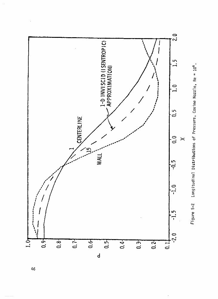
longitudinal pressure distributions along the wall and centerline are shown in
Fig. 5-2, together with the pressure distribution predicted by one dimensional
isentropic flow theory (Ref. 4) for the nozzle area variation. Pressures shown
are referred to stagnation pressure. As one might expect, the computation shows
a substantial recompression at the wall near the exit plane that is induced by the
locally concave wall shape. The inviscid core flow is supersonic in this region,
and the adverse pressure gradient causes boundary layer separation between x = 1.4
and the exit plane. The longitudinal velocity profile in the separated region is
smooth, as shown in Fig. 5-3, and displays the classic flow reversal in the near-
wall region that one expects from boundary layer theory. In the figure, velocity
is referred to the stagnation sound speed.
The vertical profiles of pressure and velocity at the geometric throat, x = 0, are
given in Figs. 5-4 and 5-5, and show substantial nonuniformities due to the two
dimensionality of the flow.
45
0.7-
0.6-
e
1-D
INVI
SCID
(IS
ENTR
OPI
C)
0.4
. , \ s \
\ 0*
3-
.
0.2-
--M
---C
-
--
0.1
I I
, I
1 ,
-2.0
-1
.5
I -1
.0
-0.5
4
0.0
0.5
1.0
1.5
2.0
X
figur
e 5-
2 Lo
ngitu
dina
l D
istri
butio
ns
of
Pres
sure
, C
osin
e N
ozzl
e,
Re
= 10
'.

CYCLE 300 TIME-15.000 K- 1 J-14 -
\ 1 I I I , \ , 1 1
: I’
I’ I’
I’ I’
I’ I’
I’ I’
I‘ I’
I’ I’
I :
1’ I’
: I‘
I’ I’
2 0.0 0.2 0.4 0.6 0.8 1.0 1.2 U V . . . w---
Figure 5-3a Velocity Profiles Across Re = 10".
Cosine Nozzle in Separated Region,
47

1 .oo////’
i
T
3 Os9’
s
/////// NOZZLE WALL
LONGITUDINAL VELOCITY, IJ
Figure 5-3b Magnified View of Longitudinal Velocity Profile in Separ'ated Region, Cosine Nozzle, Re = 105.
48

CYCLE 300 TIME-15.000 K- 1 J- 8
0 0.2 0.4 U.6 U.tl
P 0.
Figure 5-4 Pressure Profile Across Cosine Nozzle at Throat, x = 0.
49

CYf-Y .F 3-ln TTM~-~'=-I-I~I~ K- 1 .I- F)
2 0.0 0.2 0.4
u v... Mb”-
U.0 l.U
Figure 5-5 Velocity Profiles Across Cosine Nozzle at Throat, x = 0.
50
5.2 EFFECT OF IMPLICIT BOUNDARY CONDITIONS AND TIME STEPSIZE ON THE SOLUTION
5.2.1 Implicit Boundary Conditions
A set of numerical experiments has been performed to explore whether the use of
implicit boundary conditions has any significant effect on the rate of convergence
to steady state or on the final steady state solution. These tests were made for
two-dimentional laminar flow over an adiabatic flat plate at a freestream Mach Number
M, = O.l,Reynolds Number Re, = 105, Prandtl Number Pr = 1, and viscosity propor-
tional to temperature. The grid and initial conditions are as described in Ref. 1,
Section 5. In one case, implicit wall, freestream, and outflow boundary conditions
were employed as described in Ref. 1, Sections 2.4 and 4.2. In the other case,
time-lagged explicit boundary conditions were applied as follows. During each time
step, the flow variables <n+l= ;“+A$ are computed implicitly at interior grid points
by assuming that A? = 0 at boundary grid points. The flow variables at boundary
points are then updated at the end of the step by extrapolation of the solution
;jn+lfrom interior points. At wall boundary points, the velocity components (u,v,w)"+'
are set to zero and the wall pressure is computed from the normal momentum equation.
For a flat plate, the latter equation implies that the pressure gradient in the
wall-normal direction vanishes, hence the pressure at each wall point is set equal
to that at the adjacent interior point. To satisfy the adiabatic wall conditions
the gas temperature at the wall is extrapolated quadratically with zero gradient
using the temperature at the two nearest interior points along the wall-normal grid
line. At the downstream outflow boundary, 5n+1 is extrapolated linearly from the
two nearest interior points along each grid line transverse to the outflow boundary.
At the lateral outer boundary, the freestream values of pressure, temperature, and
streamwise velocity component u are imposed, and the transverse momentum f1u.x
components pv and pw are extrapolated linearly from interior points.
Numerical solutions for the two cases, implicit vs. time-lagged boundary conditions,
showed no significant difference in either convergence rate or in the final steady-
state solution as obtained with a constant time stepsize AT = 0.01. The latter
corresponds to a Courant number Co = 40 based on the minimum mesh spacing in the
direction normal to the plate. Both cases converged within 300 steps and yielded
steady-state drag coefficients that differed by only 0.07%. However, attempts
to increase the time stepsize revealed that the solution with implicit boundary
conditions remains numerically stable with time stepsizes significantly greater
51

than those attainable with time-lagged boundary conditions.
With implicit boundary conditions, the computation remains stable and converges
well for a time step as large as AT = 0.1 (Co = 400). With time-lagged boundary
conditions, the computation is unstable for AT = 0.05 (Co = 100). We have not
attempted to determine the precise stability boundaries for the two cases, because
our experi'ence has shown that the stability boundary depends upon the flow
conditions. With i& = 3, for example, the flat plate flow computation i's unstable
at AT = 0.05 (Co = 300), even with implicit boundary conditions.
As shown in the next section, the solution usually converges to steady state more
rapidly, i.e., in fewer steps, the larger the stepsize AT. Because the use of
implicit boundary conditions permits a larger stepsize, we conclude that implicit
boundary conditions significantly improve overall computational efficiency by
allowing convergence to be attained in fewer steps than would be required with
time-lagged boundary conditions.
In addition to the described experiments comparing implicit and time-lagged boundary
conditions, we have performed some test computations to evaluate the sensitivity
of the solution to the placement of the lateral outer boundary at which freestream
pressure, temperature, and streamwise velocity component, u, are imposed asboundary
conditions, but the transverse momentum components are computed implicitly from
the transverse momentum equations, The results of these tests have been reported
in detail in Ref. 9, and we merely summarize them here.
For supersonic flow, t$,>l, the solution was found to be insensitive to the location
of the outer boundary as long as the latter was positioned far enough above the .
plate to enable the shock wave generated by the viscous interaction to be captured
in the mesh.
For subsonic flow, PL,<l, the solution again was insensitive to the placement of
the outer boundary. The overall solution and the computed drag coefficient differed
by less than 0.1% when the outer boundary was shifted inward from ten boundary layer
thicknesses above the plate to as little as two boundary layerthicknesses above
the plate. The convergence histories were also virtually identical for the two cases.
Similar computations in which all freestream conditions were imposed at the lateral
outer boundary displayed a markedly different behavior. As much as a factor of
three more time steps were required to attain convergence to steady state, and the
final solution was quite sensitive to the placement of the outer boundary. The
52

computed drag coefficient was found to vary with boundary position, and the
velocity profiles within the boundary layer showed a serious distortion that did
not arise when the transverse momentum components were computed implicitly at
the outer boundary.
5.2.2 Time Stepsize
As indicated in Ref. I, a linear stability analysis shows that the implicit
numerical algorithm is unconditionally stable for arbitrarily large values of the
time step AT. In practice, we have found that for a given type of flow, there is
a limiting value of the time step beyond which the algorithm is unstable. The
instability is attributed to nonlinear effects that are unaccounted for by linear
stability theory. The evidence suggests that the instability may be associated
with the streamwise coordinate direction t;(x) in which viscous effects are small
and have been neglected in the governing equations (2.1). This hypothesis is
based on the following observations.
Let Co(<) denote the Courant number based on the inviscid flux vector F for the
streamwise 5 direction
Co(E) = (Almax AT/M. (5.1)
A where X is an eigenvalue of the Jacobian matrix F in Eq. (2.7d) and where the
maximum is taken over all five eigeuvalues and over all grid points. The Courant
numbers Co(n) and CO(G) associated with the transverse directions n,s are h similarly defined in terms of the eigenvalues of the Jacobian matrices i and H.
One can show that most explicit algorithms for the Navier-Stokes equations are
subject to the stability criterion
maxICd<), Cob-d, Co(z;)> 5 1 (5.2)
as long as the grid is locally fine enough to resolve the steep flow gradients
that exist within viscous regions such as wall boundary layers and mixing layers.
Note that the transverse Courant numbers are usually much greater than the stream-
wise one because of the much smaller transverse physical grid spacing needed to
resolve the steep transverse gradients that occur in viscous regions.
53

co(n), co(c.b~co(E) (5.3)
In contrast, the implicit algorithm remains stable for Co(n), Co(s)>>l. However,
with no artificial implicit dissipation (see Sections 2.5 and 5.4), we have found
that the implicit algorithm tends to become unstable when the streamwise Courant
number is of the order of unity or greater
unstable > O(I) (5.4)
This still gives the algorithm a great advantage over explicit schemes. For
relatively simple external and internal flows, one can obtain a crude estimate
of the stable range of AT from Eq. (5.4) when 5 = c(x) by using the approximation
Co(E) ” c(l+M)A-r/Ax (5.5)
where Ax is the physical grid spacing in the streamwise x direction and c and ki are
the dimensionless local sound speed and Mach number, respectively. For example,
for external flows such as the flat plate boundary layer addressed earlier, the
flow variables are referred to freestream conditions and Eq. (5.5) can be evaluated
at the freestream boundary c = c, = 1, M = M, using the smallest grid spacing
(AX)mi n* For internal nozzle flows where the flow variables are referred to
stagnation conditions,the streamwise grid is usually finest near the throat where
M-l,c==j/==.
External Flow Experiments
We have performed a few numerical experiments to investigate the effect of the
time stepsize on the rate of convergence for the M, = 0.1 adiabatic flat plate
boundary layer problem described in Section 5.1.1. For a 15 x 15 5-c grid, the
stable range of AT as estimated from Eq.'s (5.4) and (5.5) is
(AT) stable < 0,065
as noted in Section 5.1.1, the solution has been found to be stable for AT as
large as O.l[Co(s) = 4001 and unstable for AT = 0.5[Co(5) = 20001. Table 5.1
summarizes convergence data obtained from two computations with stepsizes that
differed by a factor of five within the stable range. The first column in the
table gives the stepsize, and the second column gives the time step number n at
which the data in the remaining columns apply. The third column gives the L2
54

residual.R,which is defined as the volume integral over the computational space of
the square of the set of steady-state terms in the Navier-Stokes equations (2.1)
and the smoothing terms, normalized by the total volume
R = 2dgdndy (5.6)
v= i
dtdndc
The factor of one-fifth is introduced so that the res i dual represents an average
over the five scalar components of the vector equation (2.1). The fourth column
in the table lists the maximum relative change over the n'th step that occurred
in any of the principal flow variables p, pu , and E at any point in the grid.
During the later stages of convergence, this turns out to be the variable pu at
one of the interior grid points adjacent to the wall. Note that this quantity
strongly affects the local velocity gradient and hence the computed wall shear
stress. This means that the computed skin friction drag represents a very
sensitive indicator of whether the solution actually has attained convergence.
The data in the last two columns of Table 5-1 are derived
fifth column contains an estimate of the
the solution I I Q/q max. The
unsteadiness in
from this value
instantaneous degree of
I 9,/q (5.7)
whereas in the last column, this quantity is scaled by the square of the time
step.
From Table 5-1, one can see that, after a given number of time steps, the solution
for the larger time step is much nearer convergence. All three measures of
convergence, the residual, the maximum relative Aq, and the degree of unsteadiness
qr/q, are much smaller for AT = 0.05 than for Ar = 0.01. The entries in the last
column of the table are nearly independent of the stepsize for a fixed number of
time steps n. This implies that, during the late stages of the calculation where
the solution is near steady state, the remaining degree of unsteadiness Iqf/qlmax
is inversely proportional to the square of the stepsize. We infer that the
convergence rate is quadratic in the stepsite A-r, and that convergence is attained
much more rapidly the larger the stepsize.
55

TABL
E 5-
l
Con
verg
ence
D
ata
for
Adia
batic
Fl
at
Plat
e Bo
unda
ry
Laye
r, M
, =
0.1,
R
e,
= 10
'
Step
size
, AT
St
ep
Num
ber,
n R
esid
ual,
R
0.01
13
7
0.05
13
7
0.01
30
0
0.05
30
0
1.53
-g
1.72
-3
1.72
-l 1.
72-’
7.90
-” 3.
15-4
6.
3-3
1.58
-’
9.70
~lo
3.24
-4
3.24
-2
3.24
-6
1.11
-l1
5.38
-’ 1.
08-3
2
.69-
6

Internal Flow Experiments --
The time stepsize also has a strong effect on the convergence rate for internal
flows. As an illustration, we present some results for a two-dimensional compu-
tation of internal laminar flow in the vertical symmetry plane of a so-called
"two-dimensional" converging-diverging nozzle that has been tested experimentally
in the static test facility of the NASA Langley 16-foot Transonic Wind Tunnel.
The nozzle configuration is described in detail in Section 6.1. We note here only
that the actual nozzle has straight sidewalls and a rectangular cross section of
constant width. The inlet section is of constant height. This is followed by a
straight-walled converging section that is connected to a straight diverging section
by a circular arc that forms the geometric throat region.
The present two-dimensional flow test computation is for nozzle operating conditions
corresponding to the nozzle design condition with a stagnation pressure of 1 atm.
and a stagnation temperature of 295 Kelvin, The Reynolds number based on stagnation
chamber conditions and throat half-height is 930,000. Although one would expect
turbulent flow at this large a Reynolds number, the computation assumes laminar
flow with a Sutherland viscosity law, a Prandtl number of 0.72, and adiabatic wall
boundary conditions. The flow is computed in the upper half of the vertical plane
of symmetry y = 0, z 2 0, which is covered by a 23x15 grid in the x(j) and z(l)
directions, respectively. The vertical (z) grid is stretched exponentially to
resolve the nozzle wall boundary layer. The initial conditions used to start
the computation were obtained in the same fashion as for the cosine nozzle test
case discussed in Section 5.1.
Two computations were performed, each starting from the same initial conditions.
The first case was run for 500 steps with a constant stepsize AT = 0.05, which
corresponds to a Courant number of 500 based on the minimum grid spacing in the
z direction. The solution at step 500 is only partially converged, as can be seen
from Figs. 5-6 and 5-7, which show the first two components of the "generalized
force vector" s (see section 3) as a function of the time step counter NC. Figure
5-6 displays FI the net mass flow through the nozzle (i.e., the difference between
the mass flows through the nozzle inlet and exit planes), normalized by the product
of the stagnation density, stagnation sound speed, and the square of the nozzle
throat half-height. The net mass flux should vanish at ateady state. The final
mass flow is out of balance by over 1.2%, and it is apparent that the solution has
not yet converged. The dimensionless thrust F2 shown in Fig. 5-7 also shows some
variation throughout the course of the run.
57

NZLT2E FSMACH=l.OOO RE=9.4+05 SMU=.OSO LMfIXBC= 1 LlBC= 1
NC
Figure 5-6 Convergence History of Net Mass Flow for 2-D Nozzle with Laminar Flow. Constant Time Stepsize Ar = 0.05.
58

NZLT2E FSMRCH=l.OOO RE=9.4+05 SMU=.OSO LMAXBC= 1 LlBC=
0.0 50.0 100.0 150.0 200.0 250.0 NC
300.0 350.0 400.0 450.0 L
Figure 5-7 Convergence History of Net Thrust for 2-D Nozzle with Laminar Flow. Constant Time Stepsize AT = 0.05.
101 3.0
59

NOZLT2 FSMACH=l.OOO RE=9.4+05 SMU=.050 LMAXBC= 1 LlBC= 1
0.0 50.0 100.0 150.0 200.0 2~10.0 300.0 350.0 400.0 450.0 5L NC
.O
Figure 5-8 Convergence History of Net Mass Flow for 2-D Nozzle with Laminar Flow. Variable Time Stepsize Increasing from AT = 0.05 to 0.3.
60

NOZLT2 FSMACH=l.OOO.RE=9.4+05 SMU=.O50 LMAXBC= I L1BC= 1
0.0 50.0 100.0 150.0 200.0 250.0 NC
300.0 350.0 400.0 450.0 5
Figure 5-9 Convergence History of Net Thrust for 2-D Nqzzle with Laminar Flow. Variable Time Stepsize Increasing from AT = 0.05 to 0.3.
61

II Ill Ill1 11111111 I II I III I 11111 I Ill1 I
Figures 5-8 and 5-9 display the corresponding results from a second 500 step run
in which the stepsize AT was increased automatically by the factor 1.1 after
each step during which the maximum relative change Aq/q max was less than 1%. I I
The stepsize increased gradually from its initial value AT = 0.05 to a maximum value
AT = 0.3 during the first 250 steps, and remained at that value for the remaining
250 steps.- The largest stepsize A-r = 0.3 corresponds to a Courant number Co(<) =
2600. The solution is essentially at steady state after 500 such increasing steps.
The final net mass flow is out of balance (Fl = 0) by less than O.OOl%, and the
thrust is steady to five significant figures. Additional results from this
converged case are given later in Section 6.1 and compared with the wind tunnel
data.
5.3 EFFECT OF ARTIFICIAL EXPLICIT SMOOTHING ON THE SOLUTION
Earlier numerical experiments with the implicit algorith showed that the solution
is not entirely insensitive to the explicit fourth-order smoothing terms which
are incorporated to control short wavelength spatial oscillations (Ref. 1, Sections
4.3 and 5.3). An array of numerical experiments has been performed to study
parametrically the variation in the steady state solution when the magnitude of
the smoothing coefficient is changed.
A set of three smoothing terms is added explicitly to the R.H.S. of Eq. (2.16a).
Each term represents a conservative fourth-order difference operator acting in
one of the three coordinate directions S,n,<. According to a linear stability
analysis (Ref. 1, Section 4.3), the coefficients of these terms are subject to
the stability criterion
82 (BiAT) [l+Ki] 5 1 i=l
(5.8a)
(5.8b)
where Xi, i = 1, 2, 3 represent the three directions E;,n,<, @AT denotes the
smoothing coefficient for each direction, and N = 2 or 3 for'two or three-
dimensional flow. In the numerical implementation, the product 6 I+Ki is 1 1 taken to be the same for all directions. The stability bound on'the coefficient
for each direction then is
62
I / 7 ! : i .:
@iAT ( 1/8N(l+Ki)
We define a relative smoothing coefficient SMU as
(5.9)
WI = BiAT/(BiAT)max (5.10)
where (8iAT)max denotes the upper bound obtained by invoking the equality in
(5.9). The quantity SMU is used as an input to the computer program to specify
the smoothing coefficient (BiAT) for each direction as a fraction of the maxi-
mum stable value determined by inequality (5.9)
BiAT = SMU/8N(l+Kj) 3 0 I_ SMU 5 1 (5.11)
Note that, for-a fixed value of SMU, the magnitude of the explicit smoothing
terms relative to the actual spatially differentiated terms in the Navier-Stokes
equations (2.1) depends upon the time stepsize A-c. The reason is that the
smoothing terms are appended to the R.H.S. of Eq. (2.16a), in which the true
spatially differentiated terms of the Navier-Stokes equations are multiplied by
the factor AT. This fact has been accounted for in Eq. (5.8) by defining the
coefficient (8iA-c) of the smoothing term for each direction to include AT as a
factor. The magnitudes of the artificial smoothing terms relative to the actual
terms in the Navier-Stokes equations then depends on the quantities Bi, and woul
be independent of the time stepsize if each Bi were taken as constant and inde-
pendent of AT. However; this would cause the stability criteria (5.8) or (5.9)
to be violated for sufficiently large values of A-r. In terms of the quantity
SMU, the stability criteria require that the coefficient BiAT satisfy Eq. (5.11)
d
Since Bi itself governs the magnitude of the artificial smoothing terms relative
to the actual Navier-Stokes terms, it follows from Eq. (5.11) that these relative
magnitudes will be preserved under a change in AT only when the ratio SMU/A-c is
held fixed, rather than when SMU itself is held fixed. That is, the ratio SMll/~-r
and not SMU itself governs the relative magnitudes of the smoothing terms and the
true Navier-Stokes terms.
We have performed an array of numerical experiments for the adiabatic flat plate
laminar flow problem to determine the sensitivity of the steady-state solution
to the magnitude of the smoothing strength.SMU/AT for a range of freestream Mach '
numbers 0.1 < M, 2 3.. - The Reynolds number is i05, the Prandtl number is unity,
and viscosity is proportional to the temgerature.
63 ’

Table 5-2 displays the variation in the computed steady-state drag coefficient CD
with smoothing coefficient for various freestream Mach numbers. For each t%,, the
last column in the table gives the percentage by which the drag coefficient for a
given value of SMU/A-c differs from the drag computed with SMU/AT = 1. The results
indicate that the solution is fairly insensitive to the magnitude of the smoothing
coefficient, except at the lowest Mach number considered. For very low-speed flows,
it appears that the accuracy of the solution is degraded significantly unless the
ratio SMU/A-c is of the order of unity or less.
The smoothing coefficient also was observed to have some effect on the rate of
convergence to steady state at both the lowest and highest Mach numbers considered.
Transient oscillations in CD were damped out somewhat more quickly with SMU/A-c = 10.
In the supersonic case, M, = 3, such behavior is to be expected because the
smoothing terms supply the dissipative mechanism that enables computation of the
embedded shock wave induced by the displacement effect of the viscous boundary
layer see Ref. 1, Section 5.2 . 1 5.4 EFFECT OF ARTIFICIAL IMPLICIT DISSIPATION ON STABILITY AND CONVERGENCE
It has been noted in Section 5.2.2 above that, for the "parabolized" Navier-Stokes
equations (2.1) wherein the viscous terms associated with the streamwise coordinate
5 are neglected, the implicit algorithm tends to become unstable for large time
steps AT atwhich the streamwise Courant number Co(c) is much greater than the order
of unity. We have performed some numerical experiments.which show that the intro-
duction of artificial implicit dissipation (see Section 2.4) extends the regime of
stability to Cournat numbers Co(S) >> 1 when the dissipation coefficient cx is of
the order of unity. This allows steady-state solutions to be attained in fewer
time steps because the rate of convergence is generally greater the larger the
time stepsize.
The results of these experiments for adiabatic flat plate laminar flow at various
freestream Mach numbers are summarized in Table 5-3. The table contains the
results of two runs for each Mach number Mm. The first run employed no implicit
dissipation (a = O)and a stepsize A-r for which the streamwise Courant number Co(c)
is of the order of unity. The second run used a dissipation coefficient c1 = 1
and a variable step AT, starting with the same initial flowfield and the same
initial values of AT and SMU (the explicit smoothing coefficient) as in the first
run. The time step during the second run was increased automatically by the factor
64

TABL
E 5-
2
Effe
ct
of
Expl
icit
Smoo
thin
g C
oeffi
cien
t on
St
eady
St
ate
Dra
g C
oeffi
cien
t Ad
iaba
tic
Flat
Pl
ate,
R
e,
= 10
5,
Pr
= 1,
pe
=
T
Mac
h N
o.
k AT
-
SMU
SM
U/A
T C
D x
lo
3 %
Var
iatio
n
0.1
0.05
0.
5 10
4.
1423
t3
.7
0.05
1
3.99
40
0.0
0.00
5 0.
1 3.
9831
-0
.27
0.8
0.05
0.
5 10
4.
0727
to
.45
0.05
1
4.05
46
0.0
0.00
5 0.
1 4.
0529
-0
.04
3.0
0.01
0.
1 10
4.
6633
to
.7
0.01
1
4.63
09
0.0
0.00
1 0.
1 4.
6287
-0
.05

TABL
E 5-
3
Effe
ct
of
Impl
icit
Dis
sipa
tion
(~0)
on
St
abilit
y an
d C
onve
rgen
ce
of
Adia
batic
Fl
at
Plat
e*
Boun
dary
La
yer
Com
puta
tions
R
e,
= 10
5,
Pr
= 1,
1-
1 =
T
M,
CY.
AT
i A-
cf
Cq(
S)
Co&
) C
Df
x lo
3 (N
C)f
- -
(SM
Wdf
(N
C),
0.1
0 5 -
2 5 -
2 0.
77
2.0t
2 1.
0 3.
9940
1
277
1 5 -
2 2.
4+'
3.7+
3 9.
8+5
3.3-
3 3.
9894
94
13
9
0.8
0 5 -
2 5 -
2 1.
25
2.0+
2 1.
0 4.
0546
1
42
1 5 -
2 1 +
2 2.
5+3
4.1t
5 8.
0-3
4.06
08
85
36
1.5
0 3
-2
3 -2
1.0
1.3+
2 1.
0 4.
1825
1
89
1 3
-2
70
2.3t
3 2.
9-
8.8-
2 4.
2028
93
12
2
* Al
l ru
ns
wer
e fo
r 20
0 st
eps

1.1 following each step during which IAq/ql,,, was less than l%, until the
time stepsize reached a pre-assigned maximum value A-rf, at which point the
stepsize was held fixed for the remainder of the run. Whenever AT was raised
in this fashion, the explicit smoothing coefficient SMU also was raised by the
same factor until it reached a maximum value SMU = 0.8. The latter bound was
imposed to avoid violating the stability criterion for the smoothing terms
[Eq. (5.11) of Section 5.31. The various columns in Table 5-3 list in order
the freestream Mach number &; the initial and final stepsizes ATi and A-rf;
the streamwise Courant number Cof(S) as estimated from Eq. (5.5) using*ATf;
the Courant number Cof(s) based on A-rf, on the maximum eigenvalue of ah/a:,
and on the minimum grid spacing in the wall normal direction; the final value
of the explicit smoothing strength (SMU/A-r)f; the final drag Coefficient CUf
at the last time step of the run; the time step index (NC)f at which the time
stepsize reached its maximum value ATf; and the time step index (NC)S at
which the drag coefficient first attained a value within tO.l% of CUf and
stayed in that range for the remainder of the run. This last entry in the
table has been included merely to provide some quantitative measure of the
convergence rate. Note that, for a given Mm, the final values of CUf differ
slightly between the runs with fixed and variable stepsize AT because the
ratio (SMU/A-c)f could not be held fixed and still satisfy the stability
criterion (5.11) in the variable-step run.
For each freestream Mach number in the table, a run of fixed stepsize AT for
which Co(<) = 10 was attempted without implicit dissipation (a = 10) and was
found to be unstable. In contrast, all of the variable-step runs with ct = 1
remained stable and converged rapidly for a maximum value of Cof(S) 4 3000.
The drag coefficient histories for these three runs are displayed in Figs. 5-10
to 5-12. We haven't determined the maximum value of Co(<) that can be attained
with c1 = 1 for various Mach numbers. However, an attempted variable-step run
at M, = 0.1 with no pre-assigned bound on AT eventually became unstable at a
value Co(c) somewhat in excess of 4000.
Implicit dissipation is potentially useful only for obtaining steady-state solutions.
The artificial terms destroy the time-accuracy of the computation and lead to a
physically unrealistic transient behavior. Neither does the implicit dissipation
always ensure either stability or faster convergence to steady state. For
67

l-7 ‘0 0 FSMRCH= .lOO GAM=1.40 RE=l.O+OS SMU=.050 LMAXBC= 2 LlBC- 1
\
3 ;
I I I I I I I I I 0 20.0 40.0 60.0 80.0 100.0 120.0 140.0 160.0 180.0 2c
NC .O
figure 5-10 Flat Plate Drag Coefficient History Computed with Implicit Dissipation cx = 1, (AT)~~~ = 240. M, = 0.1, Re, = 105.
68

0 FSMACH= .800 GAM=1.40 RE=1.0+05 SMU=.O50 LMf?XBC= 2 LlBC= 1
0 , I I I 1 I 8 I I
.O 20.0 40.0 60.0 80.0 100.0 120.0 140.0 160.0 180.0 200.0 NC
Figure 5-11 Flat Plate Drag Coefficient History Computed with Implicit Dissipation c1 = 1, (AT)~~~ = 100. M, = 0.8, Re, = 105.
69

I?
‘0 0 BL8B FSMACH=l.SOO RE=l.O+OS SMU=.030 LMAXBC= 2 LlBC= 1
0.1 I I I I I I I I I
1 20.0 40.0 60.0 80.0 100.0 120.0 140.0 160.0 180.0 2( NC
.O
Figure 5-12' Flat Plate Drag Coefficient History Computed with Implicit Dissipation a = 1, (AT),,,~~ = 70. IL= 1.5, R%, = 10 .
70

example, we performed a run at M, = 3 using IX = 1 and a constant stepsize
AT = 0.01 Co(<) 1
= 0.561 that failed to reach steady state in 200 steps; whereas,
as indicated in line 5 of Table 5-3, the corresponding run with c1 = 0 converged
adequately in the same number of steps. A similar run for M,, = 3 with an increasing
stepsize became unstable at A-r = 0.02. This suggests that the implicit dissipation
described in Section 2.4 may have a destabilizing effect for supersonic flows
with embedded shock waves. In another example, an internal nozzle flow computation
starting from very crude initial flowfield conditions proved unstable with c1 = 1
for a small, fixed stepsize AT Co(S) = 1
11, but was stable with cx = 0. In the
light of the results shown in Table 5-3, these examples suggest that the implicit
dissipation can enhance both stability and convergence for subsonic and transonic
flows if very large time steps are employed, and if the initial conditions either
are approximately correct, or are first regularized by a short preliminary run
with cx = 0 using shorter time steps. The applicability of implicit dissipation
to supersonic flows with embedded shock waves requires further investigation.
5.5 CONCLUSIONS
The principal conclusions that have emerged from the numerical experiments described
in the preceding subsections are summarized below.
1.
2.
3.
It has been demonstrated that the implicit numerical method is capable of
computing viscous flows with boundary layer separation.
Implicit boundary conditions are superior to explicit time-lagged boundary
conditions in that they allow the use of larger time stepsize without
numerical instability. For external flows, implicit freestream boundary
conditions wherein the momentum components transverse to the boundary are
computed implicitly from the transverse momentum equations are vastly
superior to the simple method where all freestream conditions are imposed
at the freestream boundary. The latter conditions retard convergence to
steady state, and seriously degrade the accuracy of the computed flowfield.
In general, larger time stepsizes give faster convergence to steady state.
Although a linear stability analysis indicates the implicit algorithm to be
unconditionally stable, experience indicates that the algorithm tends to
become unstable at time stepsizes for which the streamwise Courant number
exceeds the order of unity. Numerical experiments indicate that, within
the stable range, the convergence rate is quadratic in the time stepsize.
71

4. The algorithm involves artificial explicit fourth order smoothing terms.
Numerical experiments show that the accuracy of the solution is fairly
insensitive to the magnitude of the smoothing coefficient, except for
very low-speed subsonic flows. For such flows, the accuracy is degraded
significantly unless the ratio of the smoothing coefficient to the time
stepsize is of the order of unity or less.
5. Numerical experiments indicate that, under favorable conditions, the
introduction of artificial implicit dissipation extends the regime of
numerical stability to streamwise Courant numbers far in excess of unity.
This yield faster convergence to steady state when large time stepsizes are
used (Co >> 1). However, the implicit dissipation must be used with
caution. It destroys the time-accuracy of the solution and cannot be
employed in cases where the unsteady behavior of the flow is of interest.
The present numerical experiments suggest that the implicit dissipation
is most effective for subsonic and transonic flows. Further investigation
is recommended to study its behavior for supersonic flow with embedded
shock waves.
72
NOZZLE FLOWF
SECTION 6
IELD PREDICTIONS AND COMPARISON WITH EXPER IMENTAL DATA
Laminar and turbulent flowfield computations have been performed for
several three-dimensional nozzles that have been tested experimentally in the
NASA Langley 16-foot Transonic Wind Tunnel. The first computation is for internal
flow in a so-called "two-dimensional" converging-diverging nozzle with flat
sidewalls and a rectangular cross-section. The second computation is for the
combined internal and external flowfields of a circular, converging nozzle
in a high subsonic external flow. The results of these computations are
presented below.
6.1 Internal Flow in a "Two-Dimensional" Converging-Diverging Nozzle
6.1.1 Configuration, Operating Conditions, and Computational Grid
The nozzle configuration and dimensions are shown in Fig. 6-l. The
configuration is bilaterally symmetric with flat sidewalls and a rectangular
cross section. The inlet section is of constant height. This is followed
by a straight-walled converging section that is connected to a straight-
walled diverging section by a circular arc that forms the geometric throat
region. The exit-to-throat area ratio is 1.0891 for a design exit Mach
number of 1.35: The corresponding design exit pressure and temperature from
one-dimensional isentropic flow theory are p = 0,337 and T = 0.733,
normalized by the stagnation chamber pressure and temperature, respectively.
The operating conditions correspond to the design condition with a stagnation
pressure of 1 atm. and a stagnation temperature of 295 Kelvin. The Reynolds
number based on stagnation conditions and throat half-height is 9.3 x lo5 as
computed from the Sutherland viscosity law. The working fluid is air (y = 1.4,
Pr = 0.72).
For the flow computation, the origin of the Cartesian coordinate system
is positioned at the geometric center of the throat. The x axis coincides
with the intersection of the vertical and horizontal symmetry planes.
73

L---I
-----I
------
X
-12.
5 -1
0.0
-7.5
-5
.0
-2.5
0
2.5
5.0
NO
ZZLE
W
IDTH
=
10.1
6 cm
C
OO
RD
INAT
ES
(cm
.)
R
= 2.
7374
cm
X
Z
EXIT
AR
EA
RAT
IO
= 1.
0891
-5
.778
5 3.
5202
-1.0
401
1.57
40
THR
OAT
0.
0 1.
3686
0.05
79
1.36
93
5.77
85
1.49
05
Figu
re
6-1
Con
figur
atio
n an
d C
oord
inat
es
of
Two-
Dim
ensi
onal
N
ozzl
e

The latter coincide with the coordinate planes y = 0 and z = 0. Symmetry
boundary conditions are applied at these planes, and the flow is computed in
the quarter-space y:O, ~10. The inflow boundary is positioned at x = -4 in.,
and the outflow boundary is at the nozzle exit. The flow region between
these planes, the symmetry planes, and the nozzle walls is covered by a 23 x
10 x 15 grid in the x, y, and z directions, respectively. The streamwise (x)
grid spacing is nonuniform with a relatively fine spacing near the throat,
and the grid in each cross-sectional plane is exponentially stretched in both
the y and z directions to resolve the wall boundary layers. The computational
coordinate system thus has the form 5 = S(x), n = n(y), 5 = c(z). The
transverse grid spacings Ay, AZ are several thousand times smaller at the
walls than at the symmetry planes. Side and end views of the grid are
displayed in Fig. 6-2a and 6-2b, and an orthographic projection of the
three-dimensional grid is given in Fig. 6-2~. All dimensions shown are
referred to the throat half-height.
Laminar and turbulent flow computations have been performed for two-
dimensional flow in the vertical plane of symmetry, and a laminar flow
calculation has been performed on the three-dimensional grid shown in Fig. 6.2.
All computations employ adiabatic wall boundary conditions. Initial conditions
are obtained as follows. The inviscid core flow is obtained from one-
dimensional isentropic flow theory for the nozzle area variation. These core
flow conditions are applied over the central part of the grid in each cross-
sectional plane l<R<Rmax /2, -- assuming that the local velocity vector is oriented
along the streamwise grid lines. Velocities on the remaining part of the
grid are linearly interpolated in k and a to zero at the walls. Pressure is
taken as uniform over each cross-sectional plane. Temperature in the nonuniform
velocity region near the walls is obtained from velocity through the Crocco
relation, and density follows from the equation of state. The resulting total
pressure, total temperature, and transverse (v, w) distributions over the
inflow plane are used as inflow boundary conditions for the flowfield compu-
tation (see Section 2.3.1). The numerical results of the computations are‘
presented below in dimensionless form. Dimensions are referred to the throat
half-height, which is the reference length in terms of which the Reynolds
75

K= 1
0
ni
0
d
0
0;
N
0
rd
0
T
0
l-4
0
d
-8.0 -610 -4.0 -2.0 AXIflL COORU
Figure 6-2a Side View of Computational Grid for Two-Dimensional Nozzle
76

.I = 1 VIFWFll FRflM RFAR
2.0 3.0 Y
Figure 6-2b End View of Computational Grid for Two-Dimensional Nozzle
77
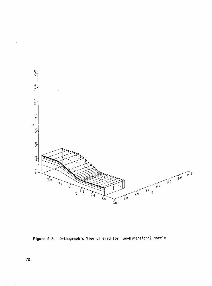
0 5
0 c; c
0 4
0 rd
rJ 0 d
C 4
6.0
Figure 6-2~ Orthographic View of Grid for Two-Dimensional Nozzle
78

number is defined. Pressure, density, and temperature are referred to the
corresponding stagnation conditions, and velocities are referred to the
stagnation sound speed.
6.1.2 Two- Dimensional Flow Results
Laminar Flow
The convergence history of this laminar flow computation has already
been discussed in Section 5.2. Convergence was attained in 500 variable time
steps. The first 100 of these were of constant size AT = 0.05, the next 70
were of increasing size, and the final 280 were constant at AT = 0.3[Co(s) = 26001.
The computation took about 3 l/2 min. of CPU time on a CDC 7600 machine. The
computed discharge coefficient is Cw = 0.9972, and the dimensionless thrust
is 7.2612. The latter is referred to po(coL)'/2 where the subscript denotes
stagnation conditions, c is the sound speed, and L is the reference length
(the throat half-height).
The nozzle wall pressure distribution is shown in Fig. 6-3, along with
preliminary experimental data from the wind tunnel test (Ref. 10). The two
sets of data represent pressure measurements on the upper and lower walls of
the test nozzle. The computed pressure distribution has the same qualitative
behavior as the data, including a slight recompression downstream of the
geometric throat. The computation is in good quantitative agreement with
the data in the subsonic and transonic region, but systematically under-
predicts the data by about 5% in the supersonic region downstream of the
throat. We shall see later that a turbulent flow computation agrees slightly
better with the data in this region.
The computed pressure distributions along the wall and the nozzle center-
line displayed in Fig. 6-4 show a substantial difference in the subsonic and
transonic region.
Turbulent Flow
The turbulent flow computation employed the converged laminar flowfield
as initial conditions. The initial stepsize AT = 0.05 increased by a factor
of 6 over the first 75 steps and was held constant for 325 more steps,
79

0 CYCLE 500 TIME- 112.3 K- 1 L-15
I I I I I I I -8.0 -6.0 -4.0 -2.0 0.0 2.0 4.0 6
X(J)
Figure 6-3 Comparison of 2-D Laminar Flow Wall Pressure Distribution With Experimental Data of Ref. 10. Data Points: Circles, Upper Flap; Triangles, Lower Flap. Computation: Solid Line.
80

CYCLE 500 TIME- 112.3 K- 1 L- 1s l---
------____
.6.0 6.
Figure 6-4 Computed Wall and Centerline Pressure Distributions for 2-D Laminar Flow. Solid Line: Wall. Dashed Line: Centerline.
81
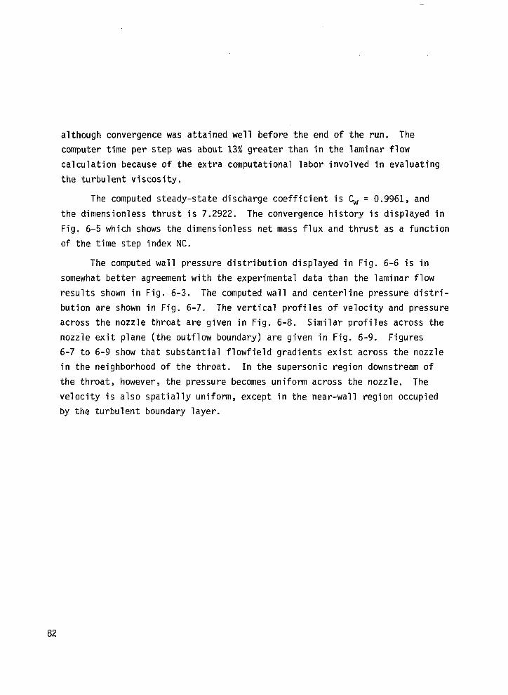
although convergence was attained well before the end of the run. The
computer time per step was about 13% greater than in the laminar flow
calculation because of the extra computational labor involved in evaluating
the turbulent viscosity.
The computed steady-state discharge coefficient is Cw = 0.9961, and
the dimensionless thrust is 7.2922. The convergence history is displayed in
Fig. 6-5 which shows the dimensionless net mass flux and thrust as a function
of the time step index NC.
The computed wall pressure distribution displayed in Fig. 6-6 is in
somewhat better agreement with the experimental data than the laminar flow
results shown in Fig. 6-3. The computed wall and centerline pressure distri-
bution are shown in Fig. 6-7. The vertical profiles of velocity and pressure
across the nozzle throat are given in Fig. 6-8. Similar profiles across the
nozzle exit plane (the outflow boundary) are given in Fig. 6-9. Figures
6-7 to 6-9 show that substantial flowfield gradients exist across the nozzle
in the neighborhood of the throat. In the supersonic region downstream of
the throat, however, the pressure becomes uniform across the nozzle, The
velocity is also spatially uniform, except in the near-wall region occupied
by the turbulent boundary layer.
82

r-0 ‘0 0 - . xh
0
rd
0
IJi
0
v
-0
-r-i
k5
0
ni
0
0
d
0
I
NOZLT2 FSMACH= .OOO RE=9.4+05 SMU=.OSO LMAXBC- 1 LlBC-
I I I I I I I 70.0 550.0 600.0 650.0 700.0 750.0 800.0 850.0 91
NC 1.0
Figure 6-5a Convergence History for 2-D Turbulent Flow Computation Showing Net Mass Flow Rate Versus Time Step Index NC.
83

NOZLT2 FSMACH=l.OOO RE=9.4+05 SMU=.OSO LMAXBC= 1 LlBC= 1
I I I I I I I
500.0 55b.o 600.0 650.0 700.0 NC
750.0 800.0 850.0 91 30
Figure 6-5b Convergence History of 2-D Turbulent Flow Computation Showing Net Thrust Versus Time Step Index NC.
84

0 CYCLE 900 TIME- 211.1 K- 1 L-15
I I I I I I
-8.0 -6.0 -4.0 -2.0 0.0 2.0 4.0 f X(J)
Figure 6-6 Comparison of 2-D Turbulent Flow Wa 11 Pressure Distribution With Experimental Data of Ref. 10. Data Points: Triangles, Lower Flap. Computation
Circles, Upper Flap; : Solid Line.
1 5
85

0 CYCLE 900 TIME- 211.1 K- 1 L- 15 I---
l-l ;
3 5
3 ;
, ;
c
c
0
c
P
C
u
c
II
0-C
0
C
P
d
N
d
d
0
d
i
8.C I I 1 1 I I
I -6.0 -4.0 -2.0 0.0 2.0 4.0 X
Figure 6-7 Computed Wall and Centerline Pressure Distributions for 2-D Turbulent Flow. Solid Line: Wall. Dashed Line: Centerline.
86

CYCLE 900 TIME- 211-l K- 1 l-14 . . a
1 : I : 1 : I : t : I :
I : I : I ; 1
I : I : I :
I : 8 : I : I : I : I : I : I : I : I : 4 : I : 1: I: 0: 0: I: 1: I: 4: I: I: I: 8: c I I
Figure 6-8a Velocity Profiles Across Computation
Throat for 2-D Turbulent Flow
87

.
CYCLE 900 TIME- 211..1 K- 1 J-14
0 0.2 0.4 0.6 0.8 1
P b.
Figure 6-8b Pressure Profile Across Throat for 2-D Turbulent Flow Computation
88

CYCLE 900 TIME- 211.1 K- 1 J-23 : I : I : I : I : I : 1 : I : I : I : I i I : ’ : ’ : ’ i: : I i I : ’ . I : I :I : I :I :I :I :I :1 :I :I :I :I :I :I :I :, :, :I :I :8 :I :1 :I :I :I :I :I :I :I :, :I :I :1 :I :I :I :, :I :I :I :I :I z 5 : : : I : f : I
,2 0.0 0.2 0.4 0.8 1.0 U V . . .
Figure 6-9a Velocity Profiles Across Exit Plane for 2-D Turbulent Flow Computation
89

CYCLE 900 TIME- 211.1 K- 1 J-23
0.0 0.2 0.4 0.6 0.8 1. P
Figure 6-9b Pressure Profile Across Exit Plane for 2-D Turbulent Flow Computation
90

6.1.3 Three-Dimensional Flow Results
A three-dimensional laminar flow computation was performed on the
grid shown in Fig. 6-2. The computation was run for 500 time steps, by which
time the computed pressure field was essentially converged and was in agreement
with the two-dimensional flow solution at the vertical plane of symmetry. The
maximum Courant number (based on the minimum transverse mesh spacing) varied
from 94 to 516 over the course of the run, which took approximately one hour
of CDC 7600 computer time. The computed net thrust and discharge coefficient
are 7.2197 and 0.9774, respectively. Both are somewhat lower than the two-
dimensional flow predictions, which do not account for the sidewall.
Figure 6-10 shows a comparison of the computed wall pressures with
experimental data. The pressure distribution along the upper nozzle wall at
the vertical plane of symmetry is given in Fig. 6-10a. The corresponding
pressure distribution along the sidewall at the horizontal plane of symmetry
is displayed in Fig. 6-lob. As for the two-dimensional results, the compu-
tation tends to underpredict the data downstream of the throat, but agrees
closely with the data in the subsonic and transonic regions upstream of the
throat.
The computed flowfield is smooth, regular, and shows no evidence of
boundary layer separation over most of the nozzle interior. However, the
flowfield contains a strong secondary flow in the neighborhood of the axial
corner where the upper wall and sidewall intersect. This secondary flow is
localized in the throat region -0.88 5 x 5 0.6 (see Fig. 6-2a), and displays
a flow reversal. Near the upstream and downstream ends of the described x
interval, the velocity profiles near the axial corner display a slight flow
reversal that is reminiscent of the reverse flow profile in a separated
boundary layer. However, there is no flow reversal over the bulk of the
upper wall or sidewall except in the immediate neighborhood of the corner.
The peak reverse velocity exists at an axial station just upstream of the
throat (x = -0.186), and is about 100% greater in magnitude than the general
streamwise velocity V,=O.8 along the nozzle centerline at the same x station.
The secondary flow thus is more properly characterized as a reverse jet rather
than as a region of separated flow. The jet-like structure is readily apparent
in Figs. 6-lla, b, which show the computed velocity profiles in the cross-
sectional plane x = -0.186. Figs. 6-lla,b display the velocity profile along a
vertical grid line Y = const. that passes approximately through the peak
velocity point of the jet. Figs.. 6?11c,d di,splay a similar profile along a
horizontal grid line Z = const. that passes approximately through the peak.
91

a CYCLE 500 TIME- 16.5 K- 1 L-15 . .
-8.0 -6.0 -4.0 -2.0 0.0 2.0 4'.0 6' XIJI
Figure 6-10a Computed Pressure Distribution Along Upper Nozzle Wall at Vertical Symmetry Plane Compared with Experimental Data
92
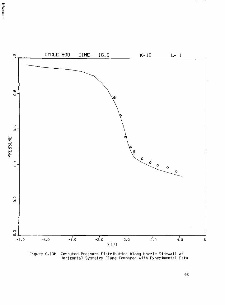
CYCLE 500 TIME- 16.5 K-10 L- 1
-
-8.0 -6.0 -4.0 -2.0 0.0 2.0 4.0 6 X(J)
Figure 6-lob Computed Pressure Distribution Along Nozzle Sidewall at Horizontal Symmetry Plane Compared with Experimental Data
93

CYCLE 500 TIME- 16.5 K- 9 J-13
0 -1.5 -1.0 -0.5 0.0 0.5 1. U V . . . w---
Figure 6-lla Velocity Profiles Along a Vertical Grid Line Passing Approximately Through Peak of Reverse Corner Jet
94

T -12 x 1o-4
5
2
s -14 x lo-4 Iu1
-16 x 10-4
. .
; . . . . . .
. : . . . . . -. . . . .
-;
. . . . . . . . .
-. . . .
\;
:
: . . .
.a .
: . . .
Figure 6-lib Magnified View of Near-Wall Portion of Velocity Profile Shown in Figure 6-lla
95

CYCLE 500 TIME- 16.5 J-13
-1.5 -1.0 -0.5 0.0 0.5 1. U V . . . w---
Figure 6-11~ Velocity Profiles Along a Horizontal Grid Line Passing Approximately Through Peak of Reverse Corner Jet
96
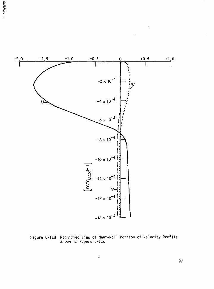
-2.0 -1.5 -1.0 -0.5 0 +0.5 +l.O
Figure 6-lld Magnified View of Near-Wall Portion of Velocity Profile Shown in Figure 6-11~
97

6.2 INTERNAL AND EXTERNAL FLOWFIELD OF A CIRCULAR NOZZLE
6.2.1 Configuration, Operating Conditions, and Computational Grid
The configuration of this axisymmetric nozzle is displayed in Fig. 6-12.
The interior wall has an inlet section of constant radius, a convergent section,
and an exit section of constant radius. The external wall consists of an initial
section of constant radius, followed by a circular arc boattail. The internal
and external surfaces do not meet at a sharp trailing edge at the exit. Rather,
the trailing edge is squared off by a vertical cut. Because the numerical
algorithm employs a Cartesian base coordinate system, axisymmetric flows must
be treated as any other three-dimensional flow; that is by using a full three-
dimensional grid. In the present case, the flow region about the nozzle is
bounded by inflow and outflow planes normal to the symmetry axis, and by a
cylindrical outer boundary (the freestream boundary) that is concentric with the
nozzle and is located 5 cm away from the cylindrical initial section of the
outer surface of the nozzle. The outflow boundary is placed about one exit
diameter downstream of the nozzle exit so as to include the near-field exhaust
jet and the wake of the nozzle wall in the computation. The first quadrant y>O,
z>O of the region between the inflow and outflow planes and within the outer - cylindrical boundary is mapped onto a rectangular computational parallelepiped
as shown in Fig. 6-13. The flow computation is carried out on a uniform
28x5~28 grid in this computational space. Note that the mapping is singular,
inasmuch as the axis of symmetry maps onto the surface <=O in the computational
space.
The image of this uniform grid in physical space consists of five meridional
planes (including the symmetry planes y=O and z=O) equally-spaced at intervals of
22.5 degrees; 28 cross-sectional planes along the x direction, of which the last
five are downstream of the nozzle exit; 15 grid points distributed exponentially
across the interior of the nozzle in the radial direction, and another 13 points
distributed exponentially between the outer surface of the nozzle wall and the
cylindrical outer boundary. Side and end views of the physical grid are displayed
in Figs. 6-14a and 6-14b.
The wind tunnel test conditions are such that both the outer and internal
flows are turbulent. The conditions are as follows (Ref. 11): Air is the medium
for both the internal and external flows (y = 1.4, Rr = 0.72). The internal flow
stagnation pressure and temperature are 1.32 atm. and 300 Kelvin, respectively.
98
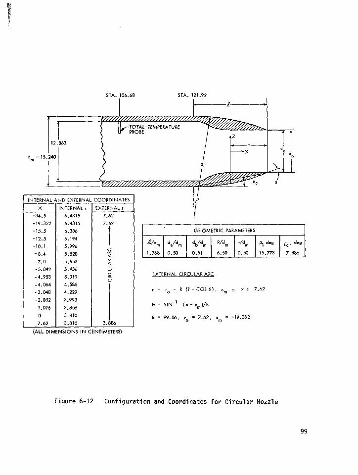
STA. 106.60 STA. 121.92
INTERNAL
X
-34.5
-19.322
-15.5
-12.5
-10.1
-a.4
-7.0
-5.842
-4.953
-4.064
-3.048
-2.032
-1.016
0
dD EXTERNAI
INTERNAL r
6.4315
6.4315
6.336
6.194
5.996
5.820
5.653
5.436
5.019
4.585
4.229
3.993
3.856
3.810
3.810
ZOORDINATES
EXTERNAL r
7.62
7.62
i
z
2
2 E u
P 3.886
IN CENTIMETERS)
I GEOMETRIC PARAMETERS
-e/d, de/d, db/d m R/d,.,, t/d,,, P, deg pc, deg 1.768 0.50 0.51 6.50 0.50 15.773 7.886
EXTERNAL CIRCULAR ARC
r = r. - R (1 - COS t?), xm L x 5 7.62
8 = SIN-’ (x - x”)/R
R = 99.06, r = 7.62, x = -19.322 0 m
Figure 6-12 Configuration and Coordinates for Circular Nozzle
99

c !l
LATE
RAL
O
UTE
R
BOU
ND
ARY
I
N 0
2 Z
L E
WAL
L ‘/
///A
g iii Z -
I I
) SY
MM
ETR
Y AX
IS
k
SID
E VI
EW
END
VI
EW
SYM
MET
RY
AXIS
*7
7
Figu
re
6-13
Ill
ustra
tion
of
Com
puta
tiona
l Sp
ace
for
Circ
ular
N
ozzl
e

3.0
4.0
-6:
0 -4
.0
-2.0
0.
0 2.
0 4
AXI%
C
OO
RD
INAT
E X
Figu
re
6-14
a Si
de
view
of
C
ompu
tatio
nal
Grid
fo
r C
ircul
ar
Noz
zle

J-l VIEWED FROM REAR
1.0 2.0 3.0
Y
Figure 6-14b End View of Computational Grid for Circular Nozzle
102

The external flow has a freestream Mach number M, = 0.8, a stagnation temperature
of 275 Kelvin, and the freestream static pressure is half the internal flow
stagnation pressure. The Reynolds number based on internal flow stagnation
chamber conditions and on the nozzle exit radius is 1.1 x 10⁶, using the
Sutherland viscosity law.
The boundary conditions for the computation are as follows: Adiabatic
wall boundary conditions are employed. The transverse velocity components
are assumed to be small over the entire inflow boundary (v = w = 0), and the
total temperature over the external flow portion of the inflow boundary is taken
as uniform and equal to the freestream stagnation temperature. Static pressure
surveys taken during the test showed no significant departure from the freestream
pressure over the external flow part of the inflow plane (Ref. 12). This
information, together with the measured external boundary layer velocity distri-
bution has been used to calculate the remaining flow variables, which are held
fixed over the external flow portion of the inflow plane during the flowfield
computation.
On the portion of the inflow plane interior to the nozzle, probe surveys
lacked the resolution to give information any more detailed than an estimate
on the boundary layer thickness on the interior wall surface (Ref. 12).
Consequently, the total temperature has been assumed uniform and equal to the
measured stagnation temperature. A one-seventh power boundary layer velocity
profile has been used together with the static pressure and core velocity
predicted by one-dimensional isentropic flow theory to estimate the total pressure
distribution across the part of the inflow plane interior to the nozzle. The
described total pressure and total temperature are used as boundary conditions
for the implicit flowfield computation (see Section 2.3.1).
The initial conditions for the region between the inflow plane and the
nozzle exit plane are obtained as follows. Flow conditions in the interior of
the nozzle are estimated in the same fashion as described in Section 5.1 for
the cosine-shaped nozzle. Outside the nozzle, the transverse velocity components
are set to zero (v = w = 0), and both the static pressure and the total tempera-
ture are assumed uniform and equal to their freestream values. Along each
streamwise mesh line n = const., 5 = const., the total pressure is assumed
constant and equal to its value at the inflow plane. The velocity u and static
temperature T then are computed from the known total pressure, total temperature,
and static pressure, and density follows from the equation of state. The
initial conditions at grid points in the cross sectional planes downstream of
the nozzle exit plane simply are set equal to the conditions at the corresponding
103

points in the exit plane itself.
Numerical results for turbulent flow are presented below in dimensionless
form. The non-dimensionalization is as described at the end of subsection 6.1.1.
6.2.2 Numerical Results
The three-dimensional turbulent flow computation attained convergence
in 500 time steps at maximum Courant numbers (based on the minimum transverse
grid spacing) that ranged from 1400 to 6800. The computation took slightly less
than one hour of CDC 7600 computer time, and yielded a final steady state value
of 3.428 for the net thrust.
Figure 6-15 displays the computed static pressure distribution along the
interior surface of the nozzle wall and along the continuation of the wall grid
line into the downstream mixing region. A similar distribution of pressure along
the exterior surface of the nozzle wall is given in Fig. 6-16. Pressure co-
efficients derived from the latter data are shown in Fig. 6-17, along with wind
tunnel experimental data from pressure taps located along the boattail (Ref. 11).
The qualitative character of the theoretical curve matches that of the data, but
the two are in close quantitative agreement only near the aft end of the boattail.
The theoretical prediction of the crossover point from negative to positive values
of Cp lies somewhat downstream of the experimental crossover point, and the
minimum value of Cp that occurs near the forward end of the boattail is lower in
the experimental data. A similar quantitative discrepancy with data on the
forward part of the boattail was found in an axisymmetric flow solution by inves-
tigators at the Langley Research Center (according to Lawrence Putnam). In that
solution, the jet mixing region was modeled as a cylindrical sting, and only the
external flow was computed. Numerical experimentation showed that the theoreti-
cal prediction could be brought into agreement with the data by moving the upper
computational boundary (freestream boundary) farther away from the nozzle outer
surface. In the present computation, that boundary is only about 1.3 nozzle
exit radii above the forward end of the boattail, whereas the corresponding dis-
tance is 2.3 exit radii at the aft end of the boattail where the theory and
experiment agree closely. This suggests that the disagreement in the forward
region could be eliminated by shifting the freestream boundary outward a dis-
tance of about one exit radius.
104

The computed flowfield shows that the external boundary layer remains
attached over the most of the boattail, although there is a small region of
separated flow near the aft end; specifically, there is a slight flow reversal
in the velocity profiles at the last two streamwise grid points on the boattail,
as shown in Fig. 6-18. It should be noted that an earlier laminar flow compu-
tation for the same geometry and operating conditions displayed massive
separation over most of the boattail.
In addition to the boattail pressure taps, the wind tunnel test data
included total pressure probe surveys across several axial stations in the
downstream jet mixing region (Ref. 13). Figure 6-19 shows a comparison of these
data with the computed total pressure distributions along the radial grid lines
that lie nearest the probe survey stations, normalized by the computed values at the outermost interior grid point. One can see that at each station the
computed shear layer in the near wake of the nozzle wall is somewhat thinner
than that measured experimentally. This suggests that the wake turbulence
model described in Section 4 may tend to under-predict the magnitude of the
turbulent eddy viscosity in such regions.
One can also see from Fig. 6-19 that the computation apparently over-
predicts the total pressure in the inner core of the jet. This is a result of
the coarse grid employed in the region near the symmetry axis. It is anticipated
that the agreement between predicted and experimental results would be improved
substantially with the same number of grid points by using a less highly
stretched radial grid (the grid spacing at the symmetry axis is a factor of
5000 greater at the axis than at the interior nozzle wall in the present
computation), and by shifting the freestream computational boundary outward by
a distance of one nozzle exit radius.
105

CYCLE 500 TIME- 79.1
-8.0
Figure 6-15
-6.0 -4.0 -2.0 0.0 2.0 X[JI
Computed Pressure Distribution Along Interior of Nozzle Wall and Along Continuation of Wall Grid Line into Downstream Jet Mixing Region
106

0 CYCLE 500 TIME- 79.1 K- 1 L-16
03 d
N d
0 d I I I I I I
-10.0 -8.0 -6.0 -4.0 -2.0 0.0 2.0 3 XlJl
Figure 6-16 Pressure Distribution Along Exterior of Nozzle Wall Along Continuation of Wall Grid Line into Downstream
and
Jet Mixing Region
107
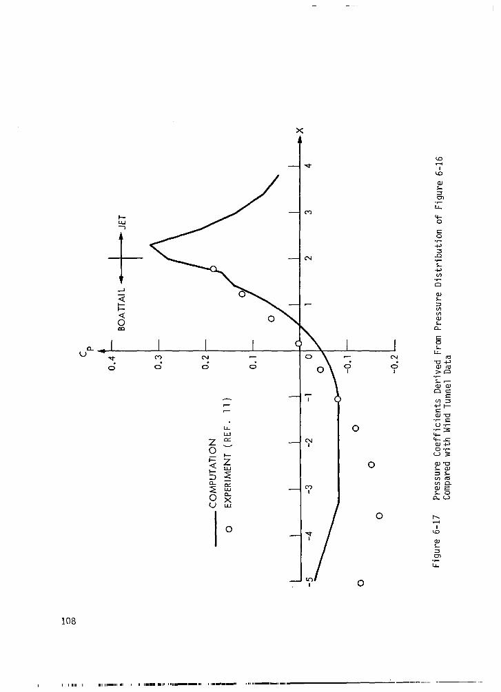
C P
CO
MPU
TATI
ON
0 EX
PER
IMEN
T (R
EF.
11)
0.4 0.3
0.2 0.
1
0 0
-0.2
BOAT
TAIL
+
JET
Figu
re
6-17
Pr
essu
re
Coe
ffici
ents
D
eriv
ed
From
Pr
essu
re
Dis
tribu
tion
of
Figu
re
6-16
C
ompa
red
with
W
ind
Tunn
el
Dat
a

CYCLE 500 TIME- 79.1
2 u. u 0.2 0.4 0.6 0.8 I U V . . . W---
Figure 6-18 Velocity Profiles Along a Vertical Grid Line at Nozzle Exit Plane, x = 2.0
109

2.5
2.0
-
0 P/P+-DATA, x=2.128 (REF. 13)
COMPUTATION,X=2.283
OL 0 0.5 1.0 1.5
NORMALIZED TOTAL PRESSURE
Figure 6-19a Comparison Between Experimental Total Pressure Probe Survey at x=2.128 With Normalized Total Pressure Profile Along the Nearest Vertical Grid Line
110

2.5
2.0
0 PT/PT,DATA, X=
-COMPUTATION,
3.128 (REF. 13')
x=3.018
0.5 1.0 I.5
NORMALIZED TOTAL PRESSURE
Figure 6-19b Comparison Between Experimental Total Pressure Probe Survey at x=3.128 with Normalized Total Pressure Profile Along the Nearest Vertical
111

L

Section 7
REFERENCES
1. Thomas, P. D.: Numerical Method for Predicting Flow Characteristics and Performance of Nonaxisymmetric Nozzles - Theory. NASA CR-3147, 1979.
2. Thomas, P. D.; and Lombard, C. K.: Geometric Conservation Law and Its Application to Flow Computations on Moving Grids. AIAA Journal, vol. 17, no. 10, Oct. 1979, pp. 1030-1037.
3. Steger, J. L.: Implicit Finite-Difference Simulation of Flow About Arbitrary Geometries. AIAA Journal, vol. 16, no. 7, July 1978.
4. Shapiro, Ascher H.: The Dynamics and Thermodynamics of Compressible Fluid Flow. Vol. I. Ronald Press Co., c.1953.
5. Franklin, P.: Methods of Advanced Calculus. McGraw-Hill, 1944, p. 123.
6. Baldwin, B. S.; and Lomax, H.: Thin Layer Approximation and Algebraic Model for Separated Turbulent Flows. AIAA Paper 78-257, Jan. 1978.
7. Schlichting, H.: Boundary Layer Theory. Fourth Ed. McGraw-Hill, 1970.
8. Thomas, P. D.; Neier, K. L.; and Middlecoff, J. F.: User's Guide for the NOZL3D Computer Program. NASA CR-159173, 1980.
9. Thomas, P. D.: Boundary Conditions for Implicit Solutions to the Compressible Navier-Stokes Equations on Finite Computational Domains. AIAA 4th Computational Fluid Dynamics Conference, Williamsburg, Va., July 1979.
10. Mason, Mary L.; Putnam, Lawrence E.; and Re, Richard J.: The Effect of Throat Contouring on Two-Dimensional Converging-Diverging Nozzles at Static Conditions. NASA TP-1704, 1980.
11. Reubush, David E.; and Runckel, Jack F.: Effect of Fineness Ratio on the Boattail Drag of Circular-Arc Afterbodies Having Closure Ratios of 0.50 With Jet Exhaust at Mach Numbers up to 1.30. NASA TN D-7192, 1973.
12. Abeyounis, William K.; and Putnam, Lawrence E.: Investigation of the Flow Field Surrounding Circular-Arc Boattail Nozzles at Subsonic Speeds. NASA TP-1633, 1980.
13. Mason, Mary L.; and Putnam, Lawrence E.: Pitot Pressure Measurements in Flow Fields Behind Circular-Arc Nozzles With Exhaust Jets at Subsonic Free-Stream Mach Numbers. NASA TM-80169, 1979.
113

_~_~~ 1. Report No. 2. Government Accession No. 3. Recipi&s. &alog No.
NASA CR-3264 4. Title and Subtitle 5. Report Date
NUMERICAL METHOD FOR PREDICTING FLOW CHARACTERISTICS October 1980 AND PERFORMANCE OF NONAXISYMMETRIC NOZZLES 6. Performing Organization Cods
PART 2 - APPLICATIONS __ 7. Author(s) 6. Performing Organization Report No.
P. D. Thomas LMSC-0678888 10. Work Unit No.
9. Performing Organization Name and Address
Lockheed Palo Alto Research Laboratory 11. Contract or Grant No.
3251 Hanover St. Palo Alto, California 94304
12. Sponsoring Agency Name and Address
National Aeronautics and Space Administration Washington, DC 20546
13. Type of Report and Period Covered
-=-ii
t 5. Supplementary Notes
Contract Monitor: Lawrence E. Putnam, NASA Langley Research Center Final Report
16. Abstract
The report summarizes work performed during the second phase of an effort to develop a computer-implemented numerical method for predicting the flow in and about an isolated three-dimensional jet exhaust nozzle. The approach is based on using an implicit numerical method to solve the unsteady Navier-Stokes equations in a boundary conforming curvilinear coordinate system. Recent improvements to the original numerical algorithm are summarized. Equations are given for evaluating nozzle thrust and discharge coefficient in terms of computed flowfield data. The final formulation of models that are used to simulate flow turbulence effect is presented. Results are presented from numerical experiments to explore the effect of various quantities on the rate of convergence to steady state and on the final flowfield solution. Detailed flowfield predictions for several two-and three-dimensional nozzle configurations are presented and compared with wind tunnel experimental data.
17. Key Words (Suggested by Author(s) J
Three Dimensional Flow Nonaxisymmetric Nozzles Numerical Flowfield Computation Navier-Stokes Equations
16. Distribution Statement
Unclassified-Unlimited
Subject Category 02
19. Security Classif. (of this report1 20. Security Classif. (of lhls
Unclassified Unclassified 115 A06
For sale by the National Technical lnfolmation Service, Springfield. Virginia 22161 NASA-Langley, 1980