m.sc. econometrics & management science - quantitative finance
TRANSCRIPT

M.Sc. Econometrics & Management Science -
Quantitative Finance
Comparison and evaluation of systemic risk
measuresMaster’s thesis
Nam Ju Yoon 418735
July 31st, 2017
SupervisorProf. Dr. D. van Dijk Erasmus University
S. Seijmonsbergen KPMG
Co-readerDr. X. Leng Erasmus University


Abstract
The consequences of the global financial crisis unveiled the shortcomings in the regulation
and monitoring of systemic risk. The issue with regulating and measuring systemic risk is the
fact there are many definitions and consequently many ways to quantify systemic risk. This
thesis empirically compares four methods of measuring cross-sectional systemic risk in the
European banking system (MES, ∆CoVaR, SRISK and DIP). Furthermore, relations between
these measures and the underlying banks’ characteristics are investigated using VAR method
and panel models. The different measures are shown to be good indicators of systemic risk
for the overall banking system, but show differences on individual bank level. The differ-
ences can be explained by the underlying inputs of measuring systemic risk. Market-to-book
and leverage are found to be important bank variables to consider for regulation, as these
ratios drive the systemic risk of one quarter ahead. Other bank characteristics show mixed
results across different systemic risk measures, which makes the interpretation rather difficult.
Keywords: systemic risk, risk measures, MES, SRISK, CoVaR, distress insurance premium, fi-
nancial crisis, banking system


ERASMUS UNIVERSITY ROTTERDAM
Contents
1 Introduction 5
2 Literature review 9
2.1 Definition of systemic risk . . . . . . . . . . . . . . . . . . . . . . . . . . . . . . . . . . . . 9
2.2 Systemic risk measures . . . . . . . . . . . . . . . . . . . . . . . . . . . . . . . . . . . . . . 10
2.3 Predicting systemic risk . . . . . . . . . . . . . . . . . . . . . . . . . . . . . . . . . . . . . 11
3 Data 13
4 Methodology 15
4.1 MES . . . . . . . . . . . . . . . . . . . . . . . . . . . . . . . . . . . . . . . . . . . . . . . . . 15
4.2 ∆ CoVaR . . . . . . . . . . . . . . . . . . . . . . . . . . . . . . . . . . . . . . . . . . . . . . 16
4.3 SRISK . . . . . . . . . . . . . . . . . . . . . . . . . . . . . . . . . . . . . . . . . . . . . . . . 17
4.4 DIP . . . . . . . . . . . . . . . . . . . . . . . . . . . . . . . . . . . . . . . . . . . . . . . . . . 18
4.5 Implementation . . . . . . . . . . . . . . . . . . . . . . . . . . . . . . . . . . . . . . . . . . 21
4.6 Systemic risk rankings . . . . . . . . . . . . . . . . . . . . . . . . . . . . . . . . . . . . . . 21
4.7 Evaluation with bank variables . . . . . . . . . . . . . . . . . . . . . . . . . . . . . . . . . 22
5 Empirical results - Comparing systemic risk measures 25
5.1 Comparison of systemic risk rankings . . . . . . . . . . . . . . . . . . . . . . . . . . . . . 30
5.2 Systemic risk measures for UBS and Greek banks . . . . . . . . . . . . . . . . . . . . . 34
6 Empirical results - Financial ratio’s and Systemic risk measures 37
6.1 VAR model results . . . . . . . . . . . . . . . . . . . . . . . . . . . . . . . . . . . . . . . . . 40
6.2 Panel data regression . . . . . . . . . . . . . . . . . . . . . . . . . . . . . . . . . . . . . . . 43
7 Concluding remarks 48
Appendix 54
A Literature review - systemic risk . . . . . . . . . . . . . . . . . . . . . . . . . . . . . . . . 54
B Driscoll and Kraay standard errors . . . . . . . . . . . . . . . . . . . . . . . . . . . . . . . 62
C PCA . . . . . . . . . . . . . . . . . . . . . . . . . . . . . . . . . . . . . . . . . . . . . . . . . 63
D Systemic risk ranking . . . . . . . . . . . . . . . . . . . . . . . . . . . . . . . . . . . . . . . 64
Comparison and evaluation of systemic risk measures - KPMG 4
ERASMUS UNIVERSITY ROTTERDAM
1 Introduction
The credit crunch, which arose from the bursting U.S. housing bubble in 2006 eventually led to
the global financial crisis, causing harm to financial institutions globally. This crisis in 2008, the
most severe global crisis since the 1930s, was the cause of many (near-)failures of major financial
institutions, including Bear Stearns, IndyMac, Fannie Mae, Freddie Mac and AIG. Governments
were forced to intervene and bail out certain firms that they considered either "too big to fail"
(TBTF) or "too interconnected to fail" (TITF). They feared that the failure of certain systemically
important financial institutions would lead to serious consequences to other firms and the econ-
omy. These events renewed the general interest in the definition, measurement and regulation of
systemic risk. Systemic risk can be seen as the possibility that an event at the company level can
trigger strong instability or a collapse of an entire industry or economy. Governments can then
use systemic risk as a reason to intervene in the economy. They can reduce or eliminate spillover
effects from company-level events through regulatory measures or other actions.
The financial crisis led to the bailout of AIG. At the time, AIG was considered too big to fail,
as many institutional investors were both invested in and also were insured by the company.
The institution was bailed out by the Federal government with loans of over $180 billion. It
was believed by analysts and regulators that a bankruptcy of AIG would lead to the collapse of
numerous other financial institutions. Similar to AIG, Lehman Brothers was also in danger of
insolvency. However, the government decided to not bailout Lehman Brothers resulting in the
firm’s collapse in 2008. The Federal Reserve did not have the funds to loan out money with the
risk of losing it in accordance with U.S. regulations. Even though the size of Lehman Brothers
was considered too big to fail, the Fed and the U.S. Treasury decided that a failure of Lehman
Brothers would not pose large spillover effects. This led to the largest bankruptcy filing in history.
Because of the firm’s size as well as its integration into the U.S. economy, the negative impact of
the collapse was spread throughout the financial system and the economy, leading to a systemic
crisis. These events made clear that at the time systemic risk of certain institutions could be highly
underestimated by regulators.
The consequences of the financial crisis unveiled the shortcomings in the regulation and monitor-
ing of systemic risk. In response to this, The Basel Committee on Banking Supervision proposed
a new regulatory framework, which is referred to as Basel III. The previous Basel Accords (Basel
I and Basel II) were primarily focused on the level of loss reserves that banks are required to hold
to be able to cover idiosyncratic risks that these banks face. Under Basel II, banks could either
adopt a simple methodology that applies relatively high risk weights or invest in internal models
that predict the probability of default (PD) and loss given default (LGD) of each loan or security.
Since 2007, banks that use internal models have been rewarded with lower aggregate risk weights
because regulators wanted to encourage them to invest in better risk management. Basel III in-
Comparison and evaluation of systemic risk measures - KPMG 5

ERASMUS UNIVERSITY ROTTERDAM
troduces two additional capital buffers to cover systemic risk and the risk of a bank-run, requiring
different levels of reserves for different forms of bank deposits. Next to Basel III, The Dodd-Frank
Wall Street Reform and Consumer Protection Act (Dodd-Frank) and the Solvency II Directive are
some of the other regulatory frameworks that intend to reduce systemic risks in the financial sys-
tem. The Financial Stability Oversight Council (FSOC), which was established by Dodd-Frank,
has the duty to identify and monitor risks to the U.S. financial system arising from the distress or
failure of large, financial institutions, or from risks that could arise outside the financial system.
Systemic risk can be a threat to a complete economic system. Therefore it is critical for regulators
to know in what way individual firms should contribute to managing systemic risk. It is important
that the level of regulatory capital of banks are modeled accurately, because it can take away from
a bank’s efficiency if it holds too much capital. Furthermore, policymakers should look at systemic
risks in a complete banking system, as only taking into account risks on individual level can lead
to underestimation. To implement successful regulation and monitoring, it is important to know
how to accurately measure systemic risk. However, because of its complexity, there is no clear
general definition for systemic risk among regulators, academics, practitioners and policymakers.
This makes it difficult to find a single appropriate way to accurately measure systemic risk. Any
single definition will most likely fall short and consequently any single systemic risk measure will
not be able to be the most accurate at all times as the financial system continues to evolve.
The research idea that follows from this is to empirically compare various methods of calculating
cross-sectional systemic risk measures, meaning the co-dependence of institutions on each other.
The models that regulators choose will implicitly decide their operational definition of systemic
risk. Various systemic risk measures should be analysed to be able to work out problems from
different directions. It is therefore important to know the commonalities and differences between
different systemic risk measures. Benoit et al. (2013) conduct a similar research, theoretically and
empirically comparing four major systemic risk measures that calculate the marginal contribution
of individual firms to total systemic risk (MES, SES, SRISK and ∆CoVaR) for American banks.
This thesis will add to their results by also taking into account an additional measure (DIP) and
compare the different measures on a data set of European banks. The DIP differs from the previous
measures as it is an ex ante systemic risk measure for the insurance premium against a systemic
event. It is important to note that the most effective ways to measure systemic risk may be ones
that use proprietary data that only regulators or central bankers have access to. Academia usually
do not have this data, which is why only the measures that require analytics that can be estimated
using public market data are considered.
From looking at the analytical expressions, one can look at how different models are calculated
and see what the common factors are across these measures as shown by Benoit et al. (2013). The
different components across these models can show that they have different aims or definitions for
systemic risk. Looking at empirical results of different systemic risk measures, we can see whether
Comparison and evaluation of systemic risk measures - KPMG 6
ERASMUS UNIVERSITY ROTTERDAM
the systemic risk rankings of financial institutions are similar. Here, we are particularly interested
in the Systemically Important Financial Institutions (SIFI), which are identified by the Financial
Stability Board (FSB). The globally systemically important banks (G-SIBs) are SIFI banks that
contribute most to the financial system and who’s collapse could trigger a financial crisis. Different
ways to measure and look at systemic risk can lead to differences in ranking in terms of systemic
risk contributions. In case of differences, the goal is to explain the ranking differences across the
risk measures and look at the main factors that drive these systemic risk rankings. Furthermore,
an analysis is done on time series of systemic risk measures and their dynamics for individual
banks. Especially for banks that went through a bailout or bankruptcy, it will be interesting to see
how different systemic risk measures (co-)move leading up to the event.
Even though there is a lot of literature on quantifying systemic risk and different systemic risk mea-
sures, there is not much research on whether these measures are feasible for regulation purposes.
Since there is no benchmark to compare systemic risk measures against to check their viability,
it is difficult to evaluate whether a measure is working well in practice. Acharya et al. (2012)
argue that the systemic risk measures based on expected shortfall can be seen as a substitute of
the stress tests performed by regulators. Benoit et al. (2013) conclude from discussions with
central bankers and regulators that systemic risk measures such as MES, SRISK and CoVaR are
being used for monitoring of individual firms’ systemic risk. As the empirical analysis by Benoit
et al. (2013) has shown, different systemic risk measures result in different SIFI rankings. This
implies that there are fundamental differences between the different measures and that it should
not be customary to decide on any individual measure as an input for regulation. Furthermore,
a systemic risk measure is only useful for regulatory purposes if it is able to detect systemically
important banks before they actually become a systemic threat. A serious downside of the cur-
rent systemic risk measures is that they give an individual firm’s contribution to systemic risk post
hoc, which makes them not an effective tool for regulators and policy makers. These agents are
responsible for identifying the systemically important banks to require additional capital buffers
against systemic events. For them, it would be helpful to have leading indicators as a reliable
warning for increasing systemic risk. For this reason, we test whether bank-specific variables can
act as a leading indicator to the individual systemic risk measures. To the best of our knowledge,
analyzing this relation between predictive bank characteristics and systemic risk measures is a
novelty that has not been attempted in previous research. The results should show whether a
bank’s fundamental drivers of value have some predictive power in assessing a bank’s systemic
risk contribution, which in turn would mean that they should be used for micro-prudential regu-
lation to prevent systemic events. This can also show whether the increased capital requirements,
minimum leverage ratio, and the liquidity requirements of Basel III actually help to cover systemic
risk.
This research shows that time series analysis of the four systemic risk measures, MES, ∆CoVaR,
SRISK and DIP seem to capture systemic events well as their time dynamics show to move as
Comparison and evaluation of systemic risk measures - KPMG 7

ERASMUS UNIVERSITY ROTTERDAM
expected compared to major systemic events, especially in crisis times. These measures appear to
be good indicators for overall systemic risk in the banking system. Aggregated, these measures
also show comparable dynamics over time. On individual level however, differences between the
measures become more clear. The systemic risk rankings show varying results across measures,
where it is clear that SRISK and DIP hold a bank’s size as an important factor. This also leads to
these two measures having similar rankings, while pairs with other systemic risk measures show
a relatively low commonality in rankings over time. These results show that the systemic risk
measures are important for regulators when monitoring systemic risk in the banking system as a
whole, but less reliable in identifying the most systemically important institutions.
Afterwards, banks’ systemic risk, as defined by the four measures MES, ∆CoVaR, SRISK and DIP,
are found to be driven by their market-to-book and leverage ratios. A lower market-to-book ratio
or a higher loan-to-deposit ratio of banks leads to an increase in systemic risk in the following
quarter. Other bank variables considered, such as the banks’ liquidity and performance are found
to be not a consistently driving factor of all the systemic risk measures. These results are important
novelties for research for regulators to take into account when identifying factors that trigger an
increase in systemic risk. They can react on movements in market-to-book and leverage ratios of
banks to prevent it from affecting the systemic risk in the banking system. Interestingly, relations
between systemic risk measures and bank variables can be different for banks from the PIIGS
(Portugal, Ireland, Italy, Greece and Spain) subgroup.
This thesis further consists of a literature review in section 2, which will examine different def-
initions and measures for systemic risk. Afterwards, the European bank data for the empirical
analysis will be discussed in section 3. Section 4 follows with the methodology of calculating
the four systemic risk measures and the methods used to analyze relations between these mea-
sures and bank variables. The results of the research are presented in section 5 and 6. Section 7
concludes and gives suggestions for further research.
Comparison and evaluation of systemic risk measures - KPMG 8
ERASMUS UNIVERSITY ROTTERDAM
2 Literature review
2.1 Definition of systemic risk
Because of the complexity of systemic risk, there is not one generalized definition for systemic
risk and consequently there are many different methods in literature to quantify it. Therefore, it
is important to first have a good understanding of the different existing interpretations that exist
for systemic risk.
The G10 proposed a working definition of systemic risk in their Report on Consolidation in the
Financial Sector (2001) as follows: "Systemic financial risk is the risk that an event will trigger a
loss of economic value or confidence in, and attendant increases in uncertainly about, a substantial
portion of the financial system that is serious enough to quite probably have significant adverse
effects on the real economy." The abstract terms, such as ‘a loss in confidence’ and ‘quite probably’
make it difficult to interpret the definition analytically. The Bank for International Settlements
(BIS) defines systemic risk as "the risk that the failure of a participant to meet its contractual
obligations may in turn cause other participants to default with a chain reaction leading to broader
financial difficulties." The definition proposed in the U.S. Commodity Futures Trading Commission
Glossary is: "the risk that a default by one market participant will have repercussions on other
participants due to the interlocking nature of financial markets." The European Central Bank (ECB)
refers to systemic risk in their Financial Stability Review December 2009 as "the risk that financial
instability becomes so widespread that it impairs the functioning of a financial system to the
point where economic growth and welfare suffer materially." The International Monetary Fund
(IMF), BIS and the FSB together (2009) give a definition of systemic risk as ‘a risk of disruption
to financial services that is caused by an impairment of all or parts of the financial system, which
has the potential to have serious negative consequences for the real economy.’
Also in academia, different interpretations of systemic risk can be found. Kaufman and Scott
(2003) refer to systemic risk as "the risk or probability of breakdowns in an entire system, as
opposed to breakdowns in individual parts or components, evidenced by comovements (corre-
lation) among most or all the parts." Kupiec and Nickerson (2004) define systemic risk as "the
potential for a modest economic shock to induce substantial volatility in asset prices, significant
reductions in corporate liquidity, potential bankruptcies and efficiency losses." Chan et al. (2005)
see systemic risk as the possibility of a series of correlated defaults among financial institutions -
typically banks - that occur over a short period of time, often caused by a single major event. A
formal definition is given by Billio et al. (2011) as "any set of circumstances that threatens the
stability of or public confidence in the financial system."
This partial collection of definitions for systemic risk is the cause of the many different methods to
quantify systemic risk analytically. Various risk measures exist to be able to capture the complexity
Comparison and evaluation of systemic risk measures - KPMG 9

ERASMUS UNIVERSITY ROTTERDAM
of the financial system and its risks. The common factor that is clear in each definition for systemic
risk is that there is a risk of a trigger event, which led to negative consequences in the economy.
However, these risks, trigger events and consequences are often defined differently, and sometimes
contradicting. Therefore, one should decide on what exactly is measured, in what frequency and
over what observation interval. It is important to know the distinction between triggering events
to identify where the systemic risks stem from. A more detailed literature review on the causes of
systemic risk and on why systemic risk is especially important in the financial sector can be found
in the Appendix.
2.2 Systemic risk measures
Because systemic risk is a concept with various definitions, there are many methods and mod-
els proposed by researchers to approach systemic risk. These different methods and models are
needed to be able to capture the complexity of the financial system and its risk. According to
Brunnermeier et al. (2009), a good systemic risk measure should identify the risk on the system
by individual systemic financial institutions. Largely, measuring the systemic risk contribution of
individual financial institutions can be categorized in two approaches. First, and perhaps the most
useful measures, are the ones using proprietary information on positions and risk exposures of the
financial institutions. This data is provided by financial institutions to regulators and is therefore
not easily accessible to academics. The second category focuses on market data, such as stock
returns and CDS spreads, which is publicly available. These market prices are believed to reflect
all of the publicly available information about the firms. The focus in this research will lie on the
systemic risk measures using public market data.
One way to look at different systemic risk measures is to divide them in two dimensions: the time
dimension and cross-sectional dimension (Bisias et al., 2012). The time dimension looks at how
the aggregate risk of the whole financial system changes over time, whereas the cross-sectional
dimension looks at how systemic risk is allocated over the financial institutions at one given point
in time. In the time dimension, the systemic risk stems from positive correlation of the financial
system with the economy. This can be reduced by building buffers that are countercyclical. In
the cross-sectional dimension, systemic risk arises from the interconnectedness of the financial
system and the exposures that come with it. For this problem, one should look at the individual
contribution of each financial institution to the overall systemic risk. This allocation of risk among
the institution must then be balanced as efficient as possible, to ensure that each institution pays
for the risk it imposes on the financial system. Up to this point, there has not been a systemic risk
measure that is robust and works well for both dimensions simultaneously.
In this paper, cross-sectional systemic risk measures will be compared empirically. The measures
for systemic risk commonly found in literature are:
Comparison and evaluation of systemic risk measures - KPMG 10

ERASMUS UNIVERSITY ROTTERDAM
1. Marginal expected shortfall (MES) (Acharya et al., 2010)
2. ∆CoVaR (Adrian & Brunnermeier, 2011)
3. SRISK (Brownlees & Engle, 2012)
4. Distress insurance premium (DIP), (Huang et al., 2009)
The current paper will be largely based on the methods and findings of Benoit et al. (2013), who
compare different cross-sectional systemic risk measures, both theoretically and empirically using
data on U.S. financial institutions. They find that the systemic risk measures (MES, SES, SRISK and
∆CoVaR) can be expressed as linear transformations of market risk measures, such as Expected
Shortfall (ES), Value at Risk (VaR) and firm betas. They further show that most of the variability
of the different measures can be explained by one market risk measure or firm characteristic, such
as beta, leverage and liabilities. With their empirical analysis, they try to find concordant pairs
between top 10 rankings by systemic risk measures and by firm characteristics at one time period.
The systemic risk measures are all methods that measure the potential spillover effects onto other
banks or the entire system in case of a systemic event. The disadvantage of these methods is
that they lack the additive property, that allows the individual contributions to be consistently
aggregated. For this reason, we extend the research with the DIP, which first calculates a systemic
risk indicator and then allocates the risk across the individual firms. Furthermore, the DIP takes
into account components of risk premium using CDS data, whereas the other three risk measures
are based on stock return. Another difference between these methods is that the∆CoVaR looks at
the systemic distress, conditional on the individual institutions in distress, compared to the other
three measures that focus on the individual systemic risk contribution conditional on the banking
system’s distress. The systemic risk measures will be explained in more detail in the methodology
section.
Bisias et al. (2012) collect various quantitative systemic risk measures found in literature and
divide them by data requirements. Some of the categories are macroeconomic measures, network
measures, forward-looking risk measures, stress-test measures and the already discussed cross-
sectional measures. What these different measures have in common in the way they look at
systemic risk is that the financial sector is seen as a portfolio, which consists of financial institutions
as individual assets. A more detailed description of other ways to approach systemic risk can again
be found in the Appendix.
2.3 Predicting systemic risk
There is a recent development in literature on the predictive power of macroeconomic variables
and firm characteristics on systemic risk measures. Varotto & Zhao (2014) introduce a standard-
ised version of systemic risk measures and analyse whether bank balance sheet variables can act
Comparison and evaluation of systemic risk measures - KPMG 11

ERASMUS UNIVERSITY ROTTERDAM
as early indicators to this new systemic risk measure. They find that indeed firm characteris-
tics such as size, leverage and growth in assets have predictive power on banks. They find that
these variables affect the standardised systemic risk measure differently between US banks and
European banks. Adding to bank characteristics, Laina et al. (2015) also investigate whether
macroeconomic variables can act as leading indicators of systemic banking crises in Europe, and
in particular Finland. They find that loan-to-deposit ratios and house price growth rates are the
best leading indicators for systemic risk. To our knowledge, there has not been a research on
whether the most commonly known cross-sectional systemic risk measures MES, ∆CoVaR, SRISK
and DIP can be predicted to some extent, using bank characteristics.
A large portion in literature has attempted to capture the predictability of the macroeconomy using
various systemic risk measures, since systemic events on individual level can lead to spillover to
the economy. A good systemic risk measure as an input for regulation and policy choices should
therefore have some predictive power on the macroeconomy. Giglio et al. (2016) examine 19
different measures for systemic risk, as well as a common factor using dimension reduction tech-
niques, on their predictability of macroeconomic shocks. They find that systemic risk measures
have significant prediction power out-of-sample in the lower tail of future macroeconomic shocks.
Allen et al. (2012) also propose an aggregate systemic risk measure, CATFIN, to forecast macroe-
conomic downturns using bank data. They find that CATFIN can forecast significant declines in
economic conditions six months ahead.
Comparison and evaluation of systemic risk measures - KPMG 12

ERASMUS UNIVERSITY ROTTERDAM
3 Data
For this research, the focus will be on the European banking system. For data, public market and
book data of European banks will be used. The sample will contain firms that are included in the
Stoxx Europe Banks 600 index at some point in the time sample considered. This market capital-
ization weighted index is made up of a collection of banks across 18 countries in the European
region. Next to banks from the Eurozone, this index also consists of systemically important banks
in Switzerland and the United Kingdom. The sample data will cover the period between January
2001 until December 2015, which makes the sample exactly 15 years. This allows us to see how
the European banks evolved before, during and after the financial crisis. Another criterion for the
banks included in our data sample is the size of the firms. In 2013, the European Union decided
to follow a single supervisory mechanism (SSM) for banks. The European Central Bank (ECB)
leads this SSM by monitoring the financial stability of systemically important banks. The most
significant criteria of systemic importance for direct supervision by the ECB is that the value of
the bank’s assets exceeds €30 bn. For this reason, the data sample will only include banks with
total assets that exceed this threshold at some point during the time sample. This sample further
includes banks, which emerge and/or dissolve during the time period. The full sample that results
from this consists of 86 banks from 19 European countries.
Daily stock returns of firms and the value-weighted market returns will be taken from Bloomberg.
Quarterly bank balance sheet data are taken from Datastream. Table 8 shows the sample banks
names and information, including their rank in the sample set by each characteristic. The sample
banks have an average total assets over the sample period ranging from €4.62 bn for Marfin
Investment Group to €169.98 bn for BNP Paribas. Note that the 19 European banks that are
identified as a Global Systemically Important Bank (G-SIB) by the FSB are all present in the top
25 in total assets of currently active banks. This shows that indeed size is a very important measure
for the FSB to determine systemically important banks. The average leverage ratios, calculated
as the market value of total assets (book value of debt + market value of equity) divided by the
market value of equity, range from 1.29 for GAM Holding to 465.71 for Dexia. The leverage ratio
for Dexia is exceptionally high and results from their large sovereign government bond holdings,
which resulted in Dexia becoming the first large casualty of the European sovereign debt crisis
in 2011. The average market-to-book ratio (M/B) over the sample period ranges from 0.24 for
Santander to 2.60 for Irish Bank Resolution Corporation, which was nationalized in 2009. The
average liquidity of banks, for which the loan-to-deposit ratio is used as proxy, ranges from 72.70
for Deutsche Bank to 1724.20 for Bradford & Bingley, a British bank nationalised in 2008 due
to the credit crisis. Finally, the average return on assets (RoA) of banks as profitability ranges
from -0.69 for Bank of Greece to 9.85% for Almanij, a Belgian bank that merged with KBC Group
in 2005. Furthermore, the average 5-year senior unsecured CDS spreads for the 56 available
banks are included in the table as an indication of the probability of default, which is needed to
Comparison and evaluation of systemic risk measures - KPMG 13

ERASMUS UNIVERSITY ROTTERDAM
calculate the Distress Insurance Premium. This ranges from 24.31 for Capitalia to 1021.31 for
National Bank of Greece. The summary statistics of the banks are displayed in Table 1.
Table 1 Summary statistics
Total assets Leverage M/B Liquidity Profitability
mean 315,763 15.47 1.32 225.83 0.38median 117,258 8.08 1.24 156.35 0.13max 1,699,803 465.71 2.60 1724.20 9.85min 4,617 1.29 0.24 72.70 -0.69std dev 423,168 49.41 0.47 242.50 1.46skewness 1.87 8.96 0.52 4.12 5.53kurtosis 2.71 81.96 3.08 19.51 31.10observations 3324 3093 3121 1049 3337
Note This table shows the summary statistics of the averaged bank variables over the 86 Europeanbanks across the full sample period January 2001 to December 2015. The total assets are in €m. Theleverage ratio is calculated as (book value of debt + market value of equity) divided by the marketvalue of equity. Market-to-book is the ratio of market equity value over the book equity value. Theliquidity ratio is calculated by total loans divided by total deposits. Finally, the profitability is definedas the return on assets, which is the net income divided by the average total assets as a percentage. Thedata is taken from Datastream. All data is on a quarterly frequency, except the liquidity ratio, which isyearly.
To construct the time-varying ∆CoVaR measure, the VSTOXX, German government bond yields
and swap rates are taken from Bloomberg to construct macroeconomic state variables. For each
systemic risk method, banks are excluded from the data set if the available public data needed to
construct a systemic risk measure is less than a year.
Comparison and evaluation of systemic risk measures - KPMG 14

ERASMUS UNIVERSITY ROTTERDAM
4 Methodology
To see how the financial institutions are ranked in terms of systemic risk, we compare the ranking
of the top systemically important financial institutions that are identified using each risk measure.
For this analysis, the focus here will be on the top 20 financial institutions with the highest con-
tribution to systemic risk, which is close to the number of global systemically important banks
(G-SIBs) in Europe defined by the Financial Stability Board (FSB).
The methodology follows from the methods used to calculate the respective systemic risk measures
as they are shortly explained below.
4.1 MES
The marginal expected shortfall (MES) is defined as the marginal contribution of one institution to
the systemic risk. First proposed by Acharya et al. (2010), the MES can be measured by calculating
the Expected Shortfall (ES) of the system. Formally, a financial institution’s MES is its expected
equity loss conditional on the whole financial system (market returns) taking a loss greater than its
Value-at-Risk at their α% lowest quantile. The higher the MES of a firm, the higher its individual
participation to the overall systemic risk.
Following the definition of ES, the ES of the overall banking system at time t is:
ESst(C) = Et−1(rst |rst < C) =N∑
i=1
wi tEt−1(ri t |rst < C) (1)
where rst and ri t are the market return and the returns of firm i at time t. The market return,
or the aggregate banking sector return, is the value-weighted average of all banks’ returns, rst =∑N
i=1 wi t ri t , where wi t is the relative market capitalization weight of firm i. Here, the expected
shortfall is conditional on the market return exceeding a predetermined threshold C . Then the
MES is the partial derivative of the system’s ES with respect to the weight of firm i in the system.
M ESi t(C) = −∂ ESst(C)∂ wi t
= −Et−1(ri t |rst < C) (2)
This partial derivative measures the increase in systemic risk as a cause of a marginal increase in
the weight of bank i in the system. The sign is switched to make sure that a higher MES means a
higher systemic risk to keep consistent with the other measures.
Acharya et al. (2010) then propose an extended concept of the systemic expected shortfall (SES),
which measures one financial institution’s contribution to systemic risk conditional on times of a
systemic crisis. It can be seen as the institution’s expected losses in the case that the system as a
Comparison and evaluation of systemic risk measures - KPMG 15

ERASMUS UNIVERSITY ROTTERDAM
whole is undercapitalized. This measure is however similar to the SRISK measure in construction,
which is why SES will not be included in our further analysis.
4.2 ∆ CoVaR
This method is based on the concept of VaR, which is the maximum loss within an α%-confidence
interval, and was first proposed by Adrian & Brunnermeier (2011). The CoVaR is then the VaR of
the financial system conditional on an institution-specific event C(ri t).
Pr
Xst ≤ CoVaRs|C(X i t )t |C(X i t)
= α (3)
An institution’s contribution to systemic risk is then defined as the difference between CoVaR
conditional to the institution being under distress and the CoVaR conditional on the normal state
of the institution. Again, the sign is changed for comparison reasons.
∆CoVaRi t(α) = −
CoVaRs|X i t=VaRi t (α)t − CoVaRs|X i t=Median(X i t )
t
(4)
This model uses growth rates of market valued total assets as input for the returns of the system
and individual institutions. This growth of market valued total assets for institution i is then
calculated as:
X it =
M E it · LEV i
t −M E it−1 · LEV i
t−1
M E it−1 · LEV i
t−1
(5)
where M E it is the market value of equity of the institution at time t and LEV i
t is a leverage ratio
of book value of total assets over book value of equity. The returns on the market valued total
assets of the system is then simply the returns on the average market valued total assets returns
of banks.
CoVaR is estimated using quantile regressions. First, the predicted value of the systemic asset
returns with an individual bank asset return as explanatory variable in a quantile regression gives:
X s ystem,iq = αi
q + βiqX i (6)
for the qth quantile. This quantile q is 50% for the median level. The value at risk then follows
by definition, because the value at risk, given X i is the conditional quantile.
VaRs ystemq |X i = X s ystem,i
q (7)
Then, if we have a particular predicted value for X i = VaRtq, then the CoVaR measure according
Comparison and evaluation of systemic risk measures - KPMG 16

ERASMUS UNIVERSITY ROTTERDAM
to the definition by Adrian & Brunnermeier (2011) follows as:
CoVaRs ystem|X i=VaRi
qq := VaRs ystem
q |VaRiq = α
iq + β
iqVaRi
q (8)
The constant systemic risk measure of bank i for the qth quantile is then:
∆CoVaRs ystem|iq = β i
q(VaRiq − VaRi
50%) (9)
However, the quantile regression gives a∆CoVaR measure that is constant over time. To compare
with the other systemic risk measures, we use a similar method to compute the time-varying
∆CoVaR, which can be estimated with the use of lagged state variables Mt that contain a lot of
information on time variation in asset returns. These state variables are included as conditioning
variables. The time-varying ∆CoVaR metric is computed as follows:
X it = α
i + γi Mt−1 + εit (10)
X s ystemt = αs ystem|i + β s ystem|iX i
t + γs ystem|i Mt−1 + ε
s ystem|it (11)
from which the estimated values are used to get:
VaRit(q) = α
iq + γ
iqMt−1 (12)
CoVaRit(q) = α
s ystem|i + β s ystem|iVaRit(q) + γ
s ystem|i Mt−1 (13)
From this, the time-varying ∆CoVaR is given as
∆CoVaRit(q) = CoVaRi
t(q)− CoVaRit(50%) (14)
= β s ystem|i(VaRit(q)− VaRi
t(50%)) (15)
4.3 SRISK
SRISK is a systemic risk measure proposed by Acharya et al. (2012) and Brownlees & Engle (2012)
who extend the MES to take into account both the liabilities and the size of the financial institution.
Similar to the MES, the SRISK index is the expected capital shortfall of a financial institution in
the case of a systemic event, which they define as a substantial market decline over a given time
horizon. The SRISK of a financial institution depends on its leverage degree, size and its MES. The
sum of the SRISKs of the whole financial system represents the potential capital shortfall that the
government may be pressured to recapitalize in crisis periods. Brownlees & Engle argue that the
calculation of the SRISK is similar to the stress tests that are often applied to financial institutions.
Comparison and evaluation of systemic risk measures - KPMG 17
ERASMUS UNIVERSITY ROTTERDAM
Acharya et al. (2012) define SRISK as follows:
SRISKi t = E(k(Di t + Ei t)− Ei t |C risis) (16)
= kDi t − (1− k)(1− LRM ESi,t)Ei,t (17)
where k is the prudential capital ratio. Di t is the book value of total liabilities and Ei t is the market
value of equity at time t. Equation (16) can be interpreted as a company needing enough equity to
cover k times total assets to be able to prevent a failure in the case of a crisis period. The LRM ES
is the Long Run Marginal Expected Shortfall. It is the expected loss of equity value of firm i in the
case that the market drops more than a given threshold within the next six months. According
to Acharya et al. (2012), the LRM ES can be approximated as 1− exp(−k ∗M ESi t) where M ESi t
is the one day expected loss if market returns are lower than −2%. Here, the parameter k is
estimated by extreme value theory and has been found to be close to 18. Assuming the book
value of debt will not change considerably in the next six months, the SRISK can be calculated
using Equation 17. The higher the SRISK level of a bank, the higher its capital shortfall in times of
crisis. A negative value of SRISK implies that the bank has a large enough equity buffer to protect
itself against failures. Because we will look at measuring systemic risk, we look at positive values
of SRISK as done by Brownlees & Engle (2012):
SRISKi t =max(0, kDi t − (1− k)(1− LRM ESi,t)Ei,t) (18)
4.4 DIP
The distress insurance premium is an ex ante systemic risk indicator proposed by Huang et al.
(2009) that represents the price of insurance against financial distress. The financial distress is
defined as when the financial system’s total losses exceed a given threshold. The DIP gives the
theoretical insurance premium to be charged to protect against these losses in the next 12 weeks.
The marginal contribution of each financial institution to systemic risk is a function of its size,
default probability (PD) and forecasted asset return correlations. The PD and asset correlations
need to be estimated from CDS spreads and stock price co-movements.
The first step is to calculate the one-year risk-neutral PDs of each individual bank using CDS
spreads as follows:
PDi t =atsi t
at LGDi t + btsi t(19)
where at =∫ t+T
t e−r x d x and bt =∫ t+T
t xe−r x d x , LGD the loss given default, si t the CDS spread
of bank i at time t and r the risk-free rate.
The second step is to estimate the correlation between the banks’ assets. This is done by using
Comparison and evaluation of systemic risk measures - KPMG 18

ERASMUS UNIVERSITY ROTTERDAM
Engle’s dynamic conditional correlation (DCC) method (2004) using daily stock return correlation
as a proxy for asset return correlation, assuming leverage remains constant in the short-term. This
approach is also used by Huang et al. (2012). This correlation measure is estimated as follows:
1. Let ri t be the daily stock return of bank i at time t, n the number of banks in the sample,
the conditional standard deviation is
hi t = Et−1(r2i t), ri t =Æ
hi tεi t , i = 1,2, ..., n
2. rt is a vector of daily returns of all banks on time t, rt = (r1t , r2t , ..., rnt)′. Then the condi-
tional covariance matrix of returns is defined as Et−1(rt r′t)≡ Ht
3. Then the DCC model is as follows:
Ht = DtRt Dt , with Dt = diag¦Æ
hi t
©
where Rt is the conditional correlation matrix we need.
For this method, we assume that the conditional covariance matrix of ε’s is Q t . Then qi j,t is its
i’th row, j’th column element following the GARCH(1,1) model:
qi j,t = ρi j +α(εi,t−1ε j,t−1 − ρi j) + β(qi j,t−1 − ρi j)
where ρi j is the unconditional correlation between εi t and ε j t . Then the i’th row, j’th column
element in the Rt conditional correlation matrix is
ρi j,t =qi j,tp
qii,tq j j,t
Rt is a positive definite matrix, as it is the correlation matrix from the covariance matrix Q t . Using
these statistics, the DCC model is estimated by quasi-maximum likelihood estimation method for
robustness to misspecification of the normal distribution. Then, we can model the time-varying
conditional correlation matrix Rt using the DCC model and the estimated parameters.
Finally a portfolio is constructed consisting of debt instruments issued by the banks considered,
weighted by the liability size of each bank. The risk indicator is then calculated as the risk-neutral
expectation of portfolio credit losses that equal or exceed a certain threshold level of the total
liabilities. Based on the inputs of risk-neutral PDs, correlations and liability weights, the systemic
risk indicator can be calculated by Monte Carlo simulation. The simulation is based on Tarashev
and Zhu (2008). The first part is to calculate the probability distribution of joint defaults, which
is done as follows:
1. Obtain an N × 1 vector of default thresholds using the N × 1 PDs and the assumption that
Comparison and evaluation of systemic risk measures - KPMG 19

ERASMUS UNIVERSITY ROTTERDAM
asset returns are standard normally distributed.
2. Draw an N × 1 vector from N standard normal variables of which the correlation matrix is
equal to the asset return correlation matrix. The number of values in this vector that are
smaller than the default thresholds are the number of simulated defaults for each draw.
3. Repeat this many times (500,000) to derive the probability distribution of the number of
defaults. Shown as Pr(nd = k), where k = 0, 1, ..., N and nd is the number of defaults.
The second simulation is to incorporate the LGD distribution to compute the probability distribu-
tion of portfolio losses.
1. For a given number of defaults k, draw LGDs for the default exposures 1,000 times and
compute the conditional loss distribution, Pr(T L|k) with T L the total losses.
2. Do this for each k = 1, ..., N and calculate the unconditional probability distribution of
portfolio losses as
Pr(T L) =∑
k
Pr(T L|nd = k) · Pr(nd = k) (20)
3. Using this unconditional distribution of losses, calculate the probability of an event that
the total losses are higher than α% of the total banking system liabilities. Here, we define
that a distress as a default of α% of total liabilities in the financial system, for which the
authors use 15%. The DIP is calculated by multiplying the probability with the expected
losses conditional on an event that the losses are above 15% of the total banking system
liabilities.
Huang et al. (2011) then propose a way to decompose the systemic risk into marginal risk con-
tributions of individual banks. Each marginal risk contribution is then the bank’s expected loss
conditional on a large loss for the banking system. Here, the marginal contribution to the systemic
risk indicator, the distress insurance premium is:
∂ DI P∂ Li
= E(Li|L ≥ Lmin) (21)
where L is the loss of the whole system and Li the loss of bank i. This method is similar in
calculating the marginal expected shortfall as they both look at a bank’s losses conditional on
the system falling below a certain threshold level. The sum of these marginal contributions is
again the total systemic risk, which allows for an easier risk allocation over individual banks for
regulators. To be able to include the effect of size directly, we follow Black et al. (2015), using
banks’ total liabilities as weights to calculate the marginal contribution of the DIP.
Comparison and evaluation of systemic risk measures - KPMG 20

ERASMUS UNIVERSITY ROTTERDAM
4.5 Implementation
To calculate the different systemic risk measures, certain variables and settings must be decided on
appropriately. To be able to compare these different systemic risk measures, a common framework
is needed. For MES, we set the treshold C as the 5% quantile of the market returns. The losses of
the banking system L, to calculate the marginal contributions of the DIP measure, will be set to
10% as done in Huang et al. (2011). To calculate the ∆CoVaR measure, 5%-quantile regressions
are used. The state variables included for the quantile regressions are:
1. VSTOXX, an implied volatility index based on European option prices
2. Liquidity spread, difference between the 3-month repo rate and 3-month German govern-
ment bond yield. Measures short-term liquidity risk
3. First differences of the 3-month German government bond yield
4. First differences of the slope of the yield curve, proxied by the yield spread between the
10-year and 3-month German government bond yield.
5. Simple returns on the market, STOXX Europe 600
6. The real estate sector returns in excess of the market returns
These variables should contain sufficient information on the time variation in asset returns. For
the SRISK measure, a prudential capital ratio k of 8% is taken, which follows from the papers of
Brownlees & Engle (2012) and Acharya et al. (2012). To calculate the DIP, the loss given default
is set to 55% as recommended by the Basel Accord. The 10-year Germany government bond yield
is taken as a proxy for the risk-free rate.
For this research, the rolling h-day horizon, which is needed to calculate the different systemic
measures over time, is set to one quarter (or 65 days) for all four measures.
4.6 Systemic risk rankings
The commonalities between the different average systemic risk measures can be analyzed by look-
ing at the correlations between the daily time series levels of the measures. Furthermore, a prin-
cipal component analysis (PCA) on these time series gives more insight on the common variation
across these four measures. One can also compare the systemic risk measures on the firm level,
by looking at the commonalities between the systemic risk rankings of different measures. The
differences in rankings can be displayed by calculating the concordant pair percentage between
Comparison and evaluation of systemic risk measures - KPMG 21
ERASMUS UNIVERSITY ROTTERDAM
two measures. This percentage is calculated as
#concordant pairsn(n− 1)/2
(22)
where a pair of two banks are concordant if the order of the two banks are the same in both
systemic risk measures.
4.7 Evaluation with bank variables
To test whether bank balance sheet data have some forecasting power regarding the different
systemic risk measures, we need a reasonable selection of bank-specific variables. The first bank
variable that will be considered is the leverage ratio, calculated by the market value of total assets
divided by the market value of equity. This leverage ratio, aggregated over all banks, can be seen
as the banking system’s financial strength against systemic events. A second variable to consider
is the market-to-book (M/B) ratio, calculated as the market equity value over its book equity
value. A high M/B-ratio typically means a high average return of the firm, whereas a low M/B-
ratio signifies a firm in relative distress. Therefore, a relatively low average M/B-ratio should pair
with the banking system’s aggregate systemic risk. The last variable is the loan-to-deposit (L/D)
ratio. This is a ratio often used to proxy the liquidity of a bank. Liquidity is an important factor
for Basel III as it defines how much liquid assets should be held by financial institutions. Banks
are required to hold sufficient highly-liquid assets to cover unforeseen short-term debt. Holding
too much however, means that banks are less able to lend out short-term debt. At aggregate
level, this means that a high L/D-ratio signifies a short of liquidity in a systemic crisis. Finally,
return on assets (RoA) will also be considered as a measure of profitability to see whether a bank’s
performance is linked with its systemic risk.
For this analysis, we will look at the correlation and the vector autoregression (VAR) model to see
whether the balance sheet variables have a relation and can to some extent forecast the systemic
risk measures. Using the VAR model gives the possibility to see possible relations in both direc-
tions, which could give new insights. The pth order VAR model, VAR(p), explains the evolution
of zt , which is a k× 1 vector consisting of k variables, and can be written as
zt = c + A1zt−1 + A2zt−2 + ...+ Apzt−p + et , (23)
where p is the number of lags, c is a vector of intercepts, Ai are time invariant k × k matrices
containing coefficients of the lags and et a k× 1 vector of error terms. To determine the optimal
number of lags for the VAR, we look at the models with the lowest Akaike information criterion
(AIC) and Schwarz information criterion (BIC). Because of the fact that the bank balance sheet
data are reported quarterly for most banks, the regressions are performed on quarterly basis.
Comparison and evaluation of systemic risk measures - KPMG 22

ERASMUS UNIVERSITY ROTTERDAM
Yearly data for liquidity will be linearly interpolated, whereas quarterly averages are calculated
for daily time series of the systemic risk measures. The time series first have to be tested for
stationarity, using the Augmented Dickey-Fuller test.
A panel analysis using data on each individual firm information and over time is also used. This
panel model is as follows:
yi t = αi + β′X i,t−1 + εi t , (24)
where yi t is the dependent variable, one of the four systemic risk measures, for bank i at time
t, X i,t−1 the explanatory variables lagged one quarter, αi the time-invariant individual effects of
each bank, and εi t the error term. Because we allow for the errors to be possibly correlated with
the bank variables (X i), we have to use a fixed effects estimator to deal with this endogeneity.
The fixed effect component αi , which is a random unobserved variable, captures a time-invariant
unobserved heterogeneity across banks. The fixed effects model is transformed to remove this
fixed effects component to be able to consistently estimate the general relation between systemic
risk and bank variables (β). This within-transformation is done as follows:
yi t − yi = (αi −αi) + β′(X i,t−1 − X i) + (εi t − εi) (25)
y∗i t = β′X ∗i,t−1 + ε
∗i t (26)
where yi =1T
∑Tt=1 yi t and likewise for αi and εi . The model is then estimated by OLS of y∗i
on X ∗i,t−1. To account for the fact that not every bank has available data over the complete time
period, we omit the time points with missing data in the panel data regression.
An important assumption of a fixed effects panel model is that the individual effect and the bank
variables are possibly correlated. If this is the case, the OLS estimations are biased and inconsis-
tent. Furthermore, the standard errors of the estimator are incorrect, which means that statistical
inference on these standard errors are invalid. Bertrand et al. (2004) show that conventional
standard errors are largely understated if there is indeed autocorrelation in the errors. To combat
possible heteroskedasticity and autocorrelation in the error terms, Newey & West (1987) propose
a non-parametric covariance matrix estimator which produces robust standard errors that are het-
eroskedasticity and autocorrelation consistent (HAC). Since we are using panel data, combining
both cross-sectional and time series data, the residuals from cross-sectional firms can also be cor-
related with each other. Driscoll and Kraay (1998) build on the estimation technique by Newey
& West, to also account for this so-called spatial correlation in panel data models. Therefore we
use the Driscoll and Kraay standard errors for the estimated coefficients in our panel models to
account for spatial (or cross-sectional) correlation and to make our statistical results more reli-
able. These standard errors are slightly adjusted for it to be able to be used on unbalanced panel
data. The method to obtain these standard errors are explained in the Appendix. To test for joint
Comparison and evaluation of systemic risk measures - KPMG 23

ERASMUS UNIVERSITY ROTTERDAM
significance on multiple parameters, the Wald test is used to see whether a (sub-)set of estimated
parameters are jointly different from zero.
Comparison and evaluation of systemic risk measures - KPMG 24

ERASMUS UNIVERSITY ROTTERDAM
5 Empirical results - Comparing systemic risk measures
The results for the four systemic risk measures over the past fifteen years for European banks are
shown in figure 2. The graphs show the DIP measure and the average ∆CoVaR, MES and SRISK
over the sample banks to show the overall movement of systemic risk over time.
2005 2010 2015
%
0
1
2
3
4
5
6
7MES
2005 2010 2015
%
0
0.5
1
1.5
2
2.5
3∆ CoVaR
2005 2010 20150
5
10
15
20
25
30
SRISK
2005 2010 2015
%
0
0.5
1
1.5
2
2.5
3
3.5DIP
(1) (2) (3)
(1) (2) (3)
(1) (2) (3)
(1) (2) (3)
Figure 2: Time series of average systemic risk measuresThis figure shows weekly time series of the systemic risk measures from January 2001 to December 2015.For MES,∆CoVaR and SRISK, these are averages of the measures over the 86 sample banks and DIP showsthe total Distress Insurance Premium. MES, ∆CoVaR and DIP are shown in percentages, whereas SRISK isshown in €bn. The vertical dashed lines are times of major events in the financial crisis and the Europeandebt crisis. (1) September 15th, 2008: Lehman Brothers bankruptcy. (2) May 2nd, 2010: Greek governmentbailout (3) November 30th, 2011: Federal Reserve, ECB and European central banks lower dollar swaps.
Before the comparison between the different systemic risk measures, it is good to confirm that
they are each working appropriately to monitor how systemic risk have changed over the past
fifteen years. This can be done by comparing the systemic risk time series results with systemic
and economic events as well as results found in literature. Since European data is used, compared
to U.S. data in most research papers on these systemic risk measures, differences can be a result
of systemic events on a local level.
Note that the graph for the distress insurance premium has missing data until the start of 2004.
This is due to a lack of availability in CDS data from Datastream for different banks. From 2004
on, the DIP remains relatively close to zero until the end of 2007 and the start of 2008. Overall,
spikes in systemic risk are common across all four measures can be seen, most notably during the
Comparison and evaluation of systemic risk measures - KPMG 25

ERASMUS UNIVERSITY ROTTERDAM
time of the global financial crisis of 2007 and 2008 and following the European sovereign debt
crisis of 2010. This makes sense as the global financial crisis led to the collapse and spillover of
many global systemically important financial institutions. The European sovereign debt crisis led
to failures and bailouts of many European banks, namely in Portugal, Ireland, and Greece. The
different systemic risk measures reach common peaks around the time of two systemic events
with large impact on the European banking system, the Lehman Brothers bankruptcy and the
Greek government bailout. The systemic risk starts to stabilize after the central banks lowered
swap rates to increase liquidity in the banking system. The spikes at time of systemic events show
that the systemic risk measures seem to be able to give a broad indication on the actual level of
systemic risk. The most important result is that all four measures, which are constructed from
very different methods using different input, generally show the same movements. The ∆CoVaR
measure seems to be more sensitive to other factors, such as systematic risk, than solely systemic
risk, compared to the other measures, as it is showing a lot of short-term movement.
Table 2 shows the correlation matrix between the different systemic risk measures over the com-
plete time sample. Especially between MES and∆CoVaR (81.9%) and SRISK and DIP (83.1%) are
shown to have a strong positive relation. These high correlations confirm the common movements
in these measures. Using a principal component analysis (PCA), one could summarize these risk
indices to construct a measure to better capture systemic risk and reduce noise of other factors
affecting the individual systemic risk measures. This PCA is performed on the correlation matrix
of the systemic risk measures, since the scales of the measures are very different. The principal
components of the standardized systemic risk measures are displayed in table 3 and show that
the first principal component captures 84.02% of variability across the four underlying measures.
The constructed index, the first principal component, is shown in the Appendix.
Table 2 Correlation matrix
MES ∆CoVaR SRISK DIP
MES 1.000*** 0.819*** 0.728*** 0.750***∆CoVaR 1.000*** 0.590*** 0.743***SRISK 1.000*** 0.831***DIP 1.000***
Note This table shows pairwise correlations between the daily timeseries of the systemic risk measures MES, ∆CoVaR, SRISK and DIP.For MES, ∆CoVaR, SRISK, the average over the 86 sample banks istaken. The time series run from Q1 2001 to Q4 2015, where the DIPonly has observations available from Q1 2004.
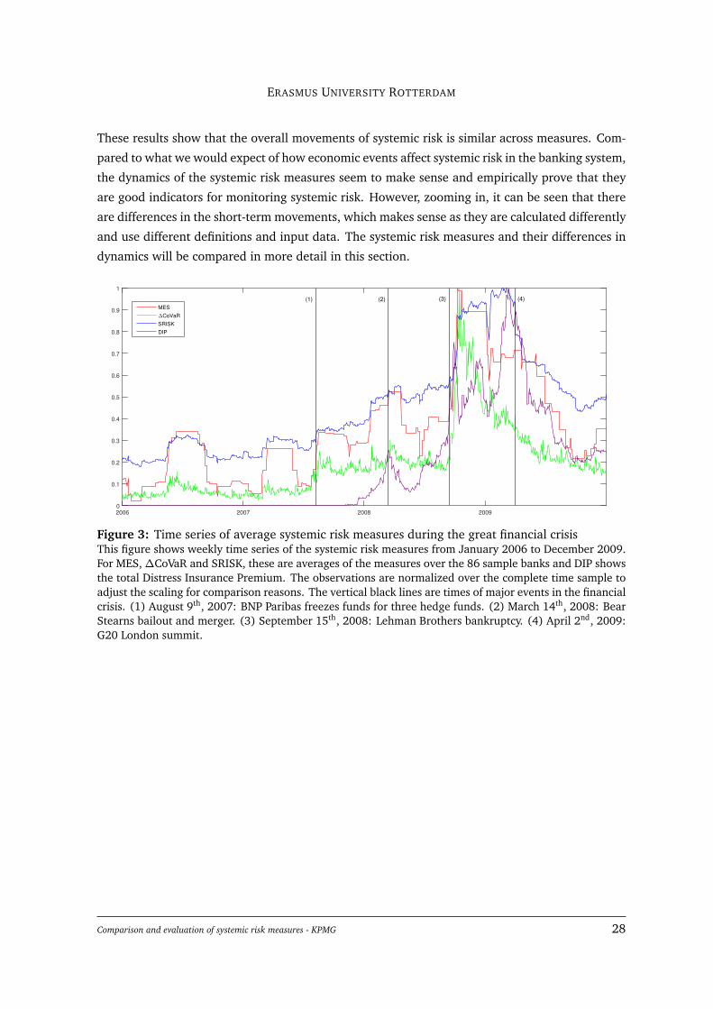
Figure 3 zooms in on the great financial crisis period and shows the movement of the systemic risk
measures. The plot also shows major events that happened during the crisis that are expected to
have had an impact on the overall European banking systemic risk. The systemic risk measures
generally seem stable before the crisis. Then they start increasing, where the measures reach a
peak at the time of the Bear Stearns acquisition. The failure of Bear Stearns came with increased
Comparison and evaluation of systemic risk measures - KPMG 26
ERASMUS UNIVERSITY ROTTERDAM
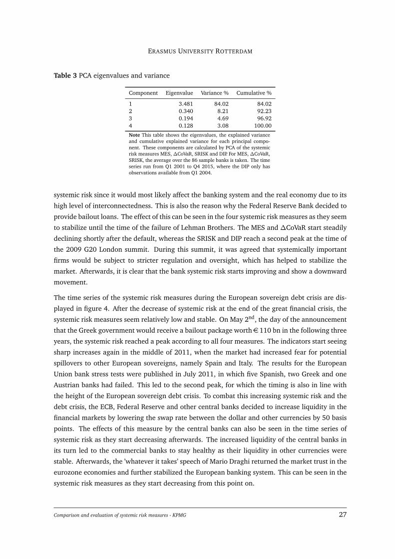
Table 3 PCA eigenvalues and variance
Component Eigenvalue Variance % Cumulative %
1 3.481 84.02 84.022 0.340 8.21 92.233 0.194 4.69 96.924 0.128 3.08 100.00
Note This table shows the eigenvalues, the explained varianceand cumulative explained variance for each principal compo-nent. These components are calculated by PCA of the systemicrisk measures MES, ∆CoVaR, SRISK and DIP. For MES, ∆CoVaR,SRISK, the average over the 86 sample banks is taken. The timeseries run from Q1 2001 to Q4 2015, where the DIP only hasobservations available from Q1 2004.
systemic risk since it would most likely affect the banking system and the real economy due to its
high level of interconnectedness. This is also the reason why the Federal Reserve Bank decided to
provide bailout loans. The effect of this can be seen in the four systemic risk measures as they seem
to stabilize until the time of the failure of Lehman Brothers. The MES and ∆CoVaR start steadily
declining shortly after the default, whereas the SRISK and DIP reach a second peak at the time of
the 2009 G20 London summit. During this summit, it was agreed that systemically important
firms would be subject to stricter regulation and oversight, which has helped to stabilize the
market. Afterwards, it is clear that the bank systemic risk starts improving and show a downward
movement.
The time series of the systemic risk measures during the European sovereign debt crisis are dis-
played in figure 4. After the decrease of systemic risk at the end of the great financial crisis, the
systemic risk measures seem relatively low and stable. On May 2nd, the day of the announcement
that the Greek government would receive a bailout package worth€110 bn in the following three
years, the systemic risk reached a peak according to all four measures. The indicators start seeing
sharp increases again in the middle of 2011, when the market had increased fear for potential
spillovers to other European sovereigns, namely Spain and Italy. The results for the European
Union bank stress tests were published in July 2011, in which five Spanish, two Greek and one
Austrian banks had failed. This led to the second peak, for which the timing is also in line with
the height of the European sovereign debt crisis. To combat this increasing systemic risk and the
debt crisis, the ECB, Federal Reserve and other central banks decided to increase liquidity in the
financial markets by lowering the swap rate between the dollar and other currencies by 50 basis
points. The effects of this measure by the central banks can also be seen in the time series of
systemic risk as they start decreasing afterwards. The increased liquidity of the central banks in
its turn led to the commercial banks to stay healthy as their liquidity in other currencies were
stable. Afterwards, the ’whatever it takes’ speech of Mario Draghi returned the market trust in the
eurozone economies and further stabilized the European banking system. This can be seen in the
systemic risk measures as they start decreasing from this point on.
Comparison and evaluation of systemic risk measures - KPMG 27
ERASMUS UNIVERSITY ROTTERDAM
These results show that the overall movements of systemic risk is similar across measures. Com-
pared to what we would expect of how economic events affect systemic risk in the banking system,
the dynamics of the systemic risk measures seem to make sense and empirically prove that they
are good indicators for monitoring systemic risk. However, zooming in, it can be seen that there
are differences in the short-term movements, which makes sense as they are calculated differently
and use different definitions and input data. The systemic risk measures and their differences in
dynamics will be compared in more detail in this section.
2006 2007 2008 20090
0.1
0.2
0.3
0.4
0.5
0.6
0.7
0.8
0.9
1
MES
∆CoVaR
SRISK
DIP
(1) (2) (3) (4)
Figure 3: Time series of average systemic risk measures during the great financial crisisThis figure shows weekly time series of the systemic risk measures from January 2006 to December 2009.For MES,∆CoVaR and SRISK, these are averages of the measures over the 86 sample banks and DIP showsthe total Distress Insurance Premium. The observations are normalized over the complete time sample toadjust the scaling for comparison reasons. The vertical black lines are times of major events in the financialcrisis. (1) August 9th, 2007: BNP Paribas freezes funds for three hedge funds. (2) March 14th, 2008: BearStearns bailout and merger. (3) September 15th, 2008: Lehman Brothers bankruptcy. (4) April 2nd, 2009:G20 London summit.
Comparison and evaluation of systemic risk measures - KPMG 28

ERASMUS UNIVERSITY ROTTERDAM
2010 2011 2012 2013 2014 20150
0.1
0.2
0.3
0.4
0.5
0.6
0.7
0.8
0.9
1
MES
∆CoVaR
SRISK
DIP
(1) (2) (3) (4) (5)
Figure 4: Time series of average systemic risk measures during the Euro sovereign debt crisisThis figure shows weekly time series of the systemic risk measures from January 2010 to December 2015.For MES,∆CoVaR and SRISK, these are averages of the measures over the 86 sample banks and DIP showsthe total Distress Insurance Premium. The observations are normalized over the complete time sample toadjust the scaling for comparison reasons. The vertical black lines are times of major events in the Eurosovereign debt crisis. (1) May 2nd, 2010: Greek government bail-out. (2) July 15th, 2011: EuropeanBanking Authority releases EU bank stress test results. (3) November 30th, 2011: Federal Reserve, ECBand European central banks lower dollar swaps. (4) July 26th, 2012: Mario Draghi’s ’whatever it takes’.(5) January 22nd, 2015: ECB announces government bond-buying program of at least €1.1 tn total.
Comparison and evaluation of systemic risk measures - KPMG 29

ERASMUS UNIVERSITY ROTTERDAM
5.1 Comparison of systemic risk rankings
To see whether different systemic risk measures result in similar results, one can look at the sys-
temic risk rankings of banks at one point in time. Table 8 shows the top 20 results of the systemic
risk rankings for each risk measure on the last time point in our sample, December 31st, 2015.
The first thing we note is that there seems to be no clear pattern across the different risk mea-
sures. Each ranking contains different banks and it is not possible to infer which banks carry more
systemic risk than others due to the differences across rankings. There is not a single bank that is
present in the top 5 ranking of all four systemic risk measures simultaneously at this time point.
Furthermore, we see in the rankings for SRISK and DIP, the banks identified as containing the
highest systemic risk tend to be the larger banks of the sample, such as BNP Paribas, Deutsche
Bank and Credit Agricole. This makes sense as many definitions of systemic risk, as well as the
Basel Committee, consider the size of a financial institution as one of the most important factors
of systemic risk. The SRISK and DIP also take the size of the bank as an important factor in cal-
culating the measures. Size seems to be of less importance in the rankings of the other two risk
measures. The MES shows two Greek banks (National Bank of Greece and Piraeus) as the ones
with the highest systemic risk. Greek banks at this time are under high pressure of default as a
result of the bank-runs in Greece following the Greek government debt crisis.
To clarify that the ranking differences between measures is not only the case at one specific time
point, Table D in the Appendix shows the rankings for a different time point (December 31st,
2010), from which we can draw the same conclusions. The different rankings especially become
clear from figure 5, which shows the percentage of concordant pairs of banks between two sys-
temic risk measures. The average concordant pair percentage over time for each pair of measures,
apart from the pair SRISK and DIP, are respectively 53.7%, 62.9%, 60.0%, 55.9%, 57.3%. This
means that about 40% of the banks are ranked in an opposite order in one systemic risk mea-
sure compared to another. For regulators using these measures, it is therefore hard to determine
which banks carry more systemic risk based on one method. Only the SRISK and DIP seem to
return very similar rankings, with an average of concordant pair percentage of 93.5%, as banks’
size is an important influence for both methods. This is due to the fact that both of these mea-
sures hold banks’ size as an important input in measuring its systemic risk contribution. The MES
and SRISK show a relatively high concordant pair percentage. This can be explained by the fact
that the SRISK is an extension of the MES, for which MES is used to approximate the long run
marginal expected shortfall (LRMES). This LRMES is used as an input for SRISK, which leads to
more similar rankings between these two measures.
To check whether the systemic risk measures individually are stable over time, one can look at the
Kendall rank correlation coefficient, taking observations at of all banks at time t and of time t−1
Comparison and evaluation of systemic risk measures - KPMG 30

ERASMUS UNIVERSITY ROTTERDAM
as a pair for each systemic risk measure. This coefficient is calculated as
τ=(#concordant pairs)− (#disconcordant pairs)
n(n− 1)/2. (27)
where a pair is called concordant if the order of the two banks are the same at both time t and t−1
and disconcordant if one bank is higher (lower) in the ranking at time t but lower (higher) in the
ranking at time t−1. The correlations are all significant over time according to the Student’s t-test.
The correlations seem to be very high, with averages of 96.7%, 95.8%, 99.3% and 99.8% for the
MES,∆CoVaR, SRISK and DIP measures. These high levels of Kendall rank correlations mean that
the rankings of the individual systemic risk measures do not change much on a day-to-day basis.
This proves that the individual measures are stable over time and that therefore the differences in
ranking across measures are the result of the underlying differences in the definitions or inputs of
the systemic risk measures. This is a desired result, as the systemically important banks identified
by each individual measure should not change drastically on a day-to-day basis.
The result that there is no clear pattern across different systemic risk measures is in line with
the systemic risk rankings of American banks, found by Benoit et al. (2013). This paper takes
a different approach to look at commonalities of the rankings between pairs of measures, by
looking at the top 10 SIFI rankings identified by each systemic risk measure and analyzing whether
these institutions are present in both rankings. They find that there is indeed a low commonality
between the top 10 systemic risk rankings of MES, ∆CoVaR and SRISK. For MES and SRISK, they
find that on average, roughly two institutions are commonly present in the top 10 rankings for
pairs of these measures. The conclusion that follows from their results is consistent with our
results, since in both analyses, the differences in the order of the rankings makes it difficult to
fully determine which banks are responsible for the most systemic risk.
This raises the question whether the existing systemic risk measures can explain the actual indi-
vidual contributions to systemic risk in the banking sector, since they all yield different results. It is
especially difficult since there is no true indicator of systemic risk and therefore no ’real’ systemic
risk to compare the different methods with. It is possible that a combination of these different
results, that approach systemic risk in different ways, can complement each other in monitoring
the real systemic risk in the banking system. Perhaps even completely new methods are needed
for regulators to give a better indication of which banks carry more systemic risk than others.
Comparison and evaluation of systemic risk measures - KPMG 31

ERASMUS UNIVERSITY ROTTERDAM
Table 4 Systemic risk rankings
Ranking MES ∆CoVaR SRISK DIP
1 National Bank Of Greece ING BNP Paribas HSBC2 Piraeus Bank Raiffeisen Bank Intl. Deutsche Bank BNP Paribas3 Allied Irish Banks Credit Suisse Credit Agricole Deutsche Bank4 Investec Banco Santander Banco Santander Credit Agricole5 Banco Portugues Invest. Deutsche Bank Commerzbank Banco Santander6 Banca Monte Dei P.S Caixabank ING Royal Bank of Scotland7 Banca Carige Nordea Bank Credit Suisse Lloyds Banking Group8 Banca Popol Emilia Rom. UBS Natixis Banques Popul. UBS9 Deutsche Bank Skandinaviska Enskilda UBS Unicredit
10 Banco Popol. Soc.Coop. Erste Group Bank Intesa Sanpaolo ING11 Ubi Banca Ubi Banca Banca Monte Dei P.S. Credit Suisse12 Banco Comercial Portug. DNB Caixabank Intesa Sanpaolo13 Commerzbank Jyske Bank Banco De Sabadell Nordea Bank14 Societe Generale Swedbank National Bank Of Greece Standard Chartered15 Banco Santander Svenska Handelsbanken Bankia Commerzbank16 Banca Bilbao Viz.Arg Commerzbank Banco Popular Espanol Natixis Banques Popul.17 Barclays GAM Holding Raiffeisen Bank Intl. Danske Bank18 Svenska Handelsbanken Banco Portugues Invest. Piraeus Bank Santander19 Julius Baer Banco Popular Espanol Ubi Banca Caixabank20 Skandinaviska Enskilda Banco Comercial Portug. Erste Group Bank Svenska Handelsbanken
Note This table shows the top 20 systemic risk rankings for each of the systemic risk measures MES,∆CoVaR, SRISK and DIP at December31st, 2015. A total of 86 European banks are considered.
Comparison and evaluation of systemic risk measures - KPMG 32

ERASMUS UNIVERSITY ROTTERDAM
2002 2004 2006 2008 2010 2012 20140
0.5
1MES and ∆CoVaR
2002 2004 2006 2008 2010 2012 20140
0.5
1MES and SRISK
2002 2004 2006 2008 2010 2012 20140
0.5
1MES and DIP
2002 2004 2006 2008 2010 2012 20140
0.5
1∆CoVaR and SRISK
2002 2004 2006 2008 2010 2012 20140
0.5
1∆CoVaR and DIP
2002 2004 2006 2008 2010 2012 20140
0.5
1SRISK and DIP
Figure 5: Percentage of concordant pairs between two systemic risk measuresThis figure shows the percentage of concordant pairs of banks between two systemic risk measures fromOctober 2001 to December 2015. Pairs of banks at a point of time are only taken into account if they areboth active and have available data. A pair of banks is considered concordant if the order of the two banksare the same in the rankings of both measures. Then the percentage of concordant pairs is calculated as#concordant pairs
n(n−1)/2 , where n is the number of banks with available data.
Comparison and evaluation of systemic risk measures - KPMG 33

ERASMUS UNIVERSITY ROTTERDAM
5.2 Systemic risk measures for UBS and Greek banks
The different results between the systemic risk measures are evident. It is however still unclear
whether these are the cause of different underlying definitions and interpretations of systemic
risk, different data inputs, or something else. Looking at individual cases could help in seeing and
understanding these differences more clearly.
Since our data covers the financial crisis of 2007/2008, it is interesting to see the dynamics of the
systemic risk measures leading up to this time. One European bank that was severe distressed in
these times is UBS. It is the bank that suffered one of the worst losses as a result of the subprime
mortgage crisis, leading to their bailout by the Swiss National Bank with funds of close to $60 bil-
lion in October 2008. Figure 6 shows the time series of the systemic risk measures for UBS from
January 2004 to December 2010. In what seems to be a calm period until the subprime mortgage
crisis in 2007, we see that the SRISK measure for UBS has large up and down movements, while
MES and ∆CoVaR stay relatively stable. This is mostly driven by the size factor, which is incor-
porated in SRISK and not in the other two measures. This period saw a large growth in size as
well as earnings. As the crisis developed further, the systemic risk in the banking system started
increasing, as can also be seen in the four systemic risk measures for UBS. All four indicators
see two peak points: one at the time that UBS announced losses of $ 37 bn, the largest losses of
any other bank at that time and afterwards at the time of the government bailout by the Swiss
National Bank. This shows that the four systemic risk measures peak similarly and can be used
to monitor systemic risk ex post. This is a good property to have for the systemic risk measures.
At the time of the bailout, UBS was in high distress and the chances of its default were high,
which is why the peaks in the systemic risk measures give a good indication of the health of the
bank. This also explains the Swiss National Bank deciding to bailout UBS, because the failure of
large systemically important bank can lead to instability in the whole banking system and/or the
economy. Furthermore, the MES, SRISK and DIP see an increase already starting from early 2007
leading up to the bailout, whereas ∆CoVaR sees a sharp increase only at the time of the event.
This could be caused by the different interpretations of systemic risk, since ∆ CoVaR calculates
the banking system’s losses conditional on the institution in distress in distress, while the other
measures look at an institution’s losses conditional on systemic distress.
Another interesting case to look at are the Greek banks during the still continuing Greek government-
debt crisis, which followed from the 2007/2008 financial crisis. We highlight Piraeus Bank and
Alpha Bank, which are the largest Greek banks in total assets and market capitalization respec-
tively. The time series of the systemic risk measures are shown in figure 7. The first thing we
note is that both banks show very similar movements for each individual method of systemic risk
measures. The movements between different measures are however very different. The MES sees
a sharp negative peak in April 2012 and at the end of 2015, but seems to be stable on a relatively
high level otherwise. SRISK shows a lot of large movements in both ways, peaking in April 2013,
Comparison and evaluation of systemic risk measures - KPMG 34

ERASMUS UNIVERSITY ROTTERDAM
2004 2005 2006 2007 2008 2009 20100
0.1
0.2
0.3
0.4
0.5
0.6
0.7
0.8
0.9
1UBS
MES
∆CoVaR
SRISK
DIP
(2)(1)
(3)
Figure 6: Time series of systemic risk measures for UBSThis figure shows the daily time series of the MES, ∆CoVaR, SRISK and the marginal contribution to DIPfor UBS from January 2001 to December 2010. The observations are normalized over the complete timesample to adjust the scaling for comparison reasons. The vertical black lines are times of major events inthe Euro sovereign debt crisis. (1) May 4th, 2007: UBS closes hedge fund. (2) May 1st, 2008: UBS doublessubprime writedowns (3) October 31st, 2008: government bailout of UBS by the Swiss National Bank.
after which it slowly decreased until Q1 2014 and has increased again towards the end of the
sample. The ∆CoVaR sees a small peak in the end of 2011, but seems very stable over the rest of
the time sample. The DIP as well peaks in the end of 2011, after which it slowly decreases and
shows a stable and relatively low systemic risk.
In the case of the Greek banks, the fundamental differences between the systemic risk measures
become more clear in the time series. It is difficult to determine whether the movements of the
different measures are the cause of purely systemic risk. Since each measure gives very different
results, it becomes unclear which systemic risk measure gives the best indication of the actual
systemic risk of Greek banks. This is another finding that supports the claim that regulators cannot
identify systemically important financial institutions based on one of these measures. The recent
developments in the Greek banking sector, which led to pressure of a Greek exit from the Eurozone,
brings along unknown risks. There are many uncertainties that follow a potential ’Grexit’. Some
of the uncertainties include investors’ reactions, the contagion effects on the Eurozone banks
and other political issues. Other countries such as countries in Southern Europe could also take
Greece’s example and leave the Eurozone, which would lead to bank-runs in these countries and
consequently a banking crisis. All these concerns and unknown risks of the future are difficult
to quantify. This could be the reason that the individual systemic risk contributions in the global
financial crisis is well captured, whereas the systemic risk for Greek banks show varying results in
the four measures.
Comparison and evaluation of systemic risk measures - KPMG 35

ERASMUS UNIVERSITY ROTTERDAM
2010 2012 20140
0.2
0.4
0.6
0.8
1Piraeus Bank
MES
∆CoVaR
SRISK
DIP
2010 2012 20140
0.2
0.4
0.6
0.8
1Alpha Bank
Figure 7: Time series of systemic risk measures for Greek banksThis figure shows the daily time series of the MES, ∆CoVaR, SRISK and the marginal contribution to DIPfor Pireaus Bank and Alpha Bank from January 2009 to December 2015. The observations are normalizedover the complete time sample to adjust the scaling for comparison reasons.
Comparison and evaluation of systemic risk measures - KPMG 36
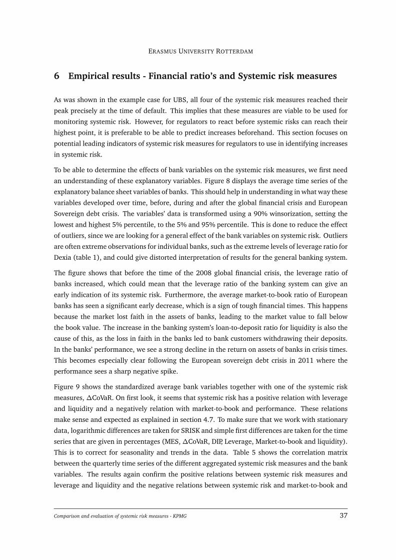
ERASMUS UNIVERSITY ROTTERDAM
6 Empirical results - Financial ratio’s and Systemic risk measures
As was shown in the example case for UBS, all four of the systemic risk measures reached their
peak precisely at the time of default. This implies that these measures are viable to be used for
monitoring systemic risk. However, for regulators to react before systemic risks can reach their
highest point, it is preferable to be able to predict increases beforehand. This section focuses on
potential leading indicators of systemic risk measures for regulators to use in identifying increases
in systemic risk.
To be able to determine the effects of bank variables on the systemic risk measures, we first need
an understanding of these explanatory variables. Figure 8 displays the average time series of the
explanatory balance sheet variables of banks. This should help in understanding in what way these
variables developed over time, before, during and after the global financial crisis and European
Sovereign debt crisis. The variables’ data is transformed using a 90% winsorization, setting the
lowest and highest 5% percentile, to the 5% and 95% percentile. This is done to reduce the effect
of outliers, since we are looking for a general effect of the bank variables on systemic risk. Outliers
are often extreme observations for individual banks, such as the extreme levels of leverage ratio for
Dexia (table 1), and could give distorted interpretation of results for the general banking system.
The figure shows that before the time of the 2008 global financial crisis, the leverage ratio of
banks increased, which could mean that the leverage ratio of the banking system can give an
early indication of its systemic risk. Furthermore, the average market-to-book ratio of European
banks has seen a significant early decrease, which is a sign of tough financial times. This happens
because the market lost faith in the assets of banks, leading to the market value to fall below
the book value. The increase in the banking system’s loan-to-deposit ratio for liquidity is also the
cause of this, as the loss in faith in the banks led to bank customers withdrawing their deposits.
In the banks’ performance, we see a strong decline in the return on assets of banks in crisis times.
This becomes especially clear following the European sovereign debt crisis in 2011 where the
performance sees a sharp negative spike.
Figure 9 shows the standardized average bank variables together with one of the systemic risk
measures, ∆CoVaR. On first look, it seems that systemic risk has a positive relation with leverage
and liquidity and a negatively relation with market-to-book and performance. These relations
make sense and expected as explained in section 4.7. To make sure that we work with stationary
data, logarithmic differences are taken for SRISK and simple first differences are taken for the time
series that are given in percentages (MES, ∆CoVaR, DIP, Leverage, Market-to-book and liquidity).
This is to correct for seasonality and trends in the data. Table 5 shows the correlation matrix
between the quarterly time series of the different aggregated systemic risk measures and the bank
variables. The results again confirm the positive relations between systemic risk measures and
leverage and liquidity and the negative relations between systemic risk and market-to-book and
Comparison and evaluation of systemic risk measures - KPMG 37

ERASMUS UNIVERSITY ROTTERDAM
2005 2010 2015
5
10
15
20
Leverage
2005 2010 20150.5
1
1.5
2
Market-to-book
2005 2010 2015140
160
180
200
220
Liquidity
2005 2010 2015
×10-3
-6
-4
-2
0
2
4Performance
Figure 8: Time series of average systemic risk measuresThis figure shows the average time series of the different bank variables over the 86 sample banks fromJanuary 2001 to December 2015. For Leverage, Market-to-Book, and Performance, quarterly reporteddata is used, whereas yearly reported data for the liquidity ratio is linearly interpolated to quarterly data.Leverage is calculated as the market value of total assets divided by market value of equity. Market-to-Bookis the book equity value divided by market equity value. Liquidity is calculated as the total loans dividedby total deposits. Performance is the return on assets.
performance. The table also shows the results of the Augmented Dickey-Fuller test for a unit root
for each of the quarterly time series. The test shows that for all the series, the null hypothesis is
rejected, which means that the data series are stationary after adjustment.
Comparison and evaluation of systemic risk measures - KPMG 38

ERASMUS UNIVERSITY ROTTERDAM
2002 2004 2006 2008 2010 2012 2014-5
-4
-3
-2
-1
0
1
2
3
4
5Bank variables and ∆CoVaR
Leverage
Market-to-Book
Liquidity
Performance
∆CoVaR
Figure 9: Time series of average systemic risk measures and ∆CoVaRThis figure shows the average time series of the different bank variables and the∆CoVaR measure over the86 sample banks from January 2001 to December 2015. For Leverage, Market-to-Book, and Performance,quarterly reported data is used, whereas yearly reported data for the liquidity ratio is linearly interpolatedto quarterly data. Leverage is calculated as the market value of total assets divided by market value ofequity. Market-to-Book is the book equity value divided by market equity value. Liquidity is calculatedas the total loans divided by total deposits. Performance is the return on assets. The observations arenormalized over the complete time sample to adjust the scaling for comparison reasons.
Table 5 Correlation matrix
MES ∆CoVaR SRISK DIP Leverage M/B Liquidity Perf.
MES 1.000*** 0.667*** 0.595*** 0.596*** 0.515*** -0.442*** -0.076 -0.104∆CoVaR 1.000*** 0.186 0.473*** 0.647*** -0.550*** -0.087 -0.138SRISK 1.000*** 0.587*** 0.297** -0.389** -0.010 -0.134DIP 1.000*** 0.445*** -0.401** 0.028 -0.057Leverage 1.000*** -0.648*** 0.072 -0.252M/B 1.000*** -0.032 -0.003Liquidity 1.000*** 0.109Perf. 1.000***
ADF-test -9.023*** -8.739*** -12.019*** -5.692*** -8.002*** -4.463*** -7.290*** -4.356***
Note This table shows pairwise correlations between the quarterly time series of the systemic risk measures MES,∆CoVaR, SRISKand DIP, and explanatory bank variables leverage, market-to-book, liquidity, and performance. For MES, ∆CoVaR, SRISK andbank variables, the average over the 86 sample banks is taken. The time series run from Q1 2001 to Q4 2015, where the DIPonly has observations available from Q1 2004. The Augmented Dickey-Fuller test statistic for each time series is also shown. Theasterisks show the rejection of the null hypothesis of a unit root on a confidence level of 1%(***), 5%(**) and 10%(*).
Comparison and evaluation of systemic risk measures - KPMG 39

ERASMUS UNIVERSITY ROTTERDAM
6.1 VAR model results
Based on the AIC and the BIC, the number of lags for the VAR model is set to 1. The results of the
VAR models are shown in table 6. We focus first on the lagged bank variables driving the future
level of systemic risk, for which we see that most of the results with the systemic risk measures as
dependent variable are insignificant. However, the F-test for the MES, SRISK and DIP regression
do show that the coefficients are jointly different from zero (MES and SRISK on 5% level and DIP
on 1% level), which means that the lagged systemic risk measure and bank variables jointly do
contain some explanatory power for the change in systemic risk one quarter forward. The F-test
for the ∆CoVaR regression does not reject the null hypothesis, implying that there is no way to
identify the coming changes in systemic risk measured by this method with the information of the
bank variables. Each covariate for ∆CoVaR is also non-significant on the 5% level.
The market-to-book ratio of banks is shown to be one of the covariates that is significant for the
other systemic risk measures, SRISK on a 5% confidence level, and MES and DIP on a 10% level.
The results show that a decreasing market-to-book ratio leads to a decrease in the systemic risk
in the following quarter. A 1% decrease in the average market-to-book ratio of the 86 sample
banks leads to a positive change in the MES level of the following quarter of 0.304%. Similar
effects are present for the SRISK and DIP, where a 1% decrease in the market-to-book ratio leads
to a positive effect in the following quarter of 0.299% and 0.315% respectively. This negative
relation makes sense as firms in high distress have low M/B-ratios. The leading aspect of the M/B
on systemic risk can also be seen in figure 9, where the average M/B ratio sees a sharp decline
already starting in June 2007, before the systemic risk measure sees the sharp increase. This
strong decline was a sign of the European banks’ stocks decreasing and consequently increasing
the banks’ systemic risk. The M/B ratio of banks, which basically says how the market views the
health of the banks, can be seen as an early warning indicator for increasing systemic risk in the
European banking sector. This is a valuable result that can be used by regulators in monitoring
and predicting systemic risk. After the crisis, the average M/B-ratio seems to be volatile on a
relatively low level of below 1 until the end of the time sample. This means that the banks are
still in high distress and therefore a high systemic risk in the European banking sector. A low
M/B-ratio often means high uncertainty in a firm’s earnings. Regulators could react to this low
and volatile market-to-book ratio by encouraging banks to focus on business models with higher
certainty of earnings. This leads to these banks being less sensitive to shocks and consequently a
lower systemic risk.
The VAR results also show a significant negative effect of liquidity to the ∆CoVaR and DIP in the
next quarter. This is unexpected as we would expect an opposite effect, since high average loan-to-
deposit ratios means the banking system is less liquid, which increases the banks’ vulnerability to
shocks and therefore leads to higher systemic risk. The other bank variables generally do not show
a significant effect on the future level of systemic risk in any method. An increase in performance
Comparison and evaluation of systemic risk measures - KPMG 40

ERASMUS UNIVERSITY ROTTERDAM
seems to have a positive effect on the average ∆CoVaR, even though an opposite relation was
expected. This positive relation could be caused by banks taking excessive risks to improve their
short-term performance, which in its turn also leads to higher systemic risk.
The VAR model also allows us to check relations with a reversed direction. In general, there is no
effect of the systemic risk measures on the bank variables one quarter ahead that is consistently
significant across all four measures. Only the ∆CoVaR seems to have a positive effect on the
European banking system’s liquidity in the following quarter. A 1% increase in the banks’ systemic
risk according to the ∆CoVaR definition leads to an increase of 0.480% in the average loan-to-
deposit ratio of European banks. Intuitively, again an opposite relation makes more sense.
Table 6 (a) VAR model results
MES Leverage M/B Liquidity Perf.
MES -0.389** -0.020 0.077 0.278 -0.093(0.147) (0.140) (0.137) (0.155) (0.133)
Leverage 0.184 -0.296 0.185 0.086 0.289**(0.186) (0.177) (0.173) (0.195) (0.168)
M/B -0.304* -0.499*** 0.643*** 0.112 0.278**(0.170) (0.161) (0.158) (0.178) (0.153)
Liquidity -0.091 -0.218* 0.130 0.024 0.128(0.126) (0.120) (0.136) (0.133) (0.114)
Performance 0.204 0.253* -0.117** 0.271*** 0.560***(0.134) (0.128) (0.137) (0.141) (0.121)
c -0.012 0.003 0.012 -0.007 -0.031(0.123) (0.117) (0.129) (0.130) (0.111)
Adjusted R2 0.129 0.215 0.244 0.042 0.276F-test 2.690** 4.124*** 4.678 1.505 5.338***
[0.030] [0.003] [0.001] [0.204] [0.000]
∆CoVaR
∆CoVaR -0.227 0.119 0.084 0.480*** -0.148(0.171) (0.166) (0.156) (0.170) (0.152)
Leverage 0.002 -0.366 0.173 -0.049 0.328*(0.199) (0.141) (0.132) (0.198) (0.177)
M/B -0.208 -0.470 0.648*** 0.166 0.262*(0.174) (0.166) (0.156) (0.173) (0.154)
Liquidity -0.239* -0.200 0.133 0.056 0.119(0.129) (0.145) (0.136) (0.128) (0.114)
Performance 0.231* 0.251 -0.117 0.270* 0.560***(0.136) (0.146) (0.137) (0.135) (0.121)
c 0.025 0.003 0.012 -0.006 -0.031(0.125) (0.136) (0.128) (0.124) (0.111)
Adjusted R2 0.067 0.223 0.244 0.118 0.282F-test 1.824 4.272 4.669 2.524** 5.476***
[0.124] [0.002] [0.001] [0.040] [0.000]
Comparison and evaluation of systemic risk measures - KPMG 41

ERASMUS UNIVERSITY ROTTERDAM
Table 6 (b) VAR model results
SRISK
SRISK -0.257** -0.019 -0.078 0.175 -0.008(0.093) (0.130) (0.127) (0.147) (0.124)
Leverage 0.046 -0.301* 0.229 0.179 0.252(0.121) (0.168) (0.165) (0.190) (0.161)
M/B -0.299** -0.501*** 0.608*** 0.102 0.292*(0.118) (0.164) (0.160) (0.185) (0.156)
Liquidity -0.069 -0.217* 0.118 -0.001 0.138(0.086) (0.119) (0.116) (0.134) (0.114)
Performance 0.143 0.256* -0.102** 0.250* 0.560***(0.093) (0.130) (0.127) (0.146) (0.124)
c -0.095 0.003 0.012 -0.008 -0.031(0.084) (0.117) (0.115) (0.133) (0.112)
Adjusted R2 0.165 0.215 0.245 0.000 0.269F-test 3.257** 4.124*** 4.693*** 0.999 5.193***
[0.012] [0.003] [0.001] [0.428] [0.001]
DIP
DIP -0.029 0.065 0.031 0.173 -0.187(0.146) (0.165) (0.152) (0.191) (0.158)
Leverage 0.177 -0.314 0.209 0.132 0.306(0.178) (0.201) (0.186) (0.233) (0.193)
M/B -0.315* -0.467** 0.648*** 0.083 0.279(0.173) (0.196) (0.181) (0.227) (0.188)
Liquidity -0.333*** -0.220 0.118 -0.012 0.129(0.117) (0.133) (0.123) (0.154) (0.127)
Performance 0.200 0.256* -0.109** 0.251*** 0.538***(0.130) (0.147) (0.135) (0.170) (0.141)
c 0.008 0.004 0.001 -0.039 -0.081(0.129) (0.147) (0.135) (0.170) (0.140)
Adjusted R2 0.258 0.182 0.228 0.037 0.240F-test 4.126*** 3.001** 3.659* 0.681 3.834***
[0.004] [0.022] [0.080] [0.641] [0.006]
Note This table shows the results of the four Vector Autoregressive (VAR) models, us-ing five standardized variables with quarterly time series: one systemic risk measurefor each model (MES, ∆CoVaR, SRISK or DIP) and the four explanatory bank vari-ables leverage, market-to-book, liquidity and performance. The estimated VAR model isyt = c + Ayt−1 + εt , where yt consists of one of the systemic risk measures or the bankvariables, c is a constant term, A is the matrix of coefficients of the lagged variables yt−1and εt is a vector of error terms. The columns show the dependent variables and the rowsshow the one-lagged explanatory variables. The asterisks show the statistical significanceof the regression coefficients on a confidence level of 1%(***), 5%(**) and 10%(*). Fi-nally, the adjusted R2 as well as the F -test statistic and its p-value (in square brackets) arereported for each regression. The F-test tests the null hypothesis of the regression coef-ficients being jointly zero. The asterisks show the rejection of this F-test on a confidencelevel of 1%(***), 5%(**) and 10%(*).
Comparison and evaluation of systemic risk measures - KPMG 42
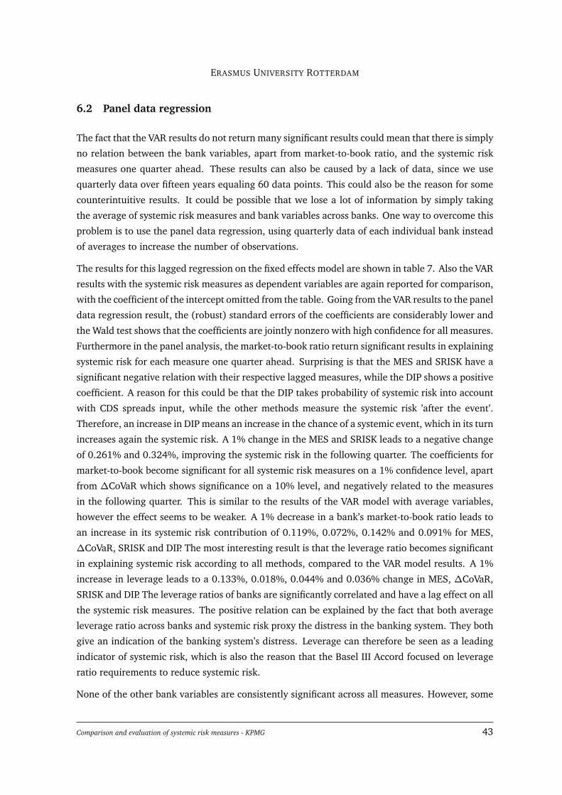
ERASMUS UNIVERSITY ROTTERDAM
6.2 Panel data regression
The fact that the VAR results do not return many significant results could mean that there is simply
no relation between the bank variables, apart from market-to-book ratio, and the systemic risk
measures one quarter ahead. These results can also be caused by a lack of data, since we use
quarterly data over fifteen years equaling 60 data points. This could also be the reason for some
counterintuitive results. It could be possible that we lose a lot of information by simply taking
the average of systemic risk measures and bank variables across banks. One way to overcome this
problem is to use the panel data regression, using quarterly data of each individual bank instead
of averages to increase the number of observations.
The results for this lagged regression on the fixed effects model are shown in table 7. Also the VAR
results with the systemic risk measures as dependent variables are again reported for comparison,
with the coefficient of the intercept omitted from the table. Going from the VAR results to the panel
data regression result, the (robust) standard errors of the coefficients are considerably lower and
the Wald test shows that the coefficients are jointly nonzero with high confidence for all measures.
Furthermore in the panel analysis, the market-to-book ratio return significant results in explaining
systemic risk for each measure one quarter ahead. Surprising is that the MES and SRISK have a
significant negative relation with their respective lagged measures, while the DIP shows a positive
coefficient. A reason for this could be that the DIP takes probability of systemic risk into account
with CDS spreads input, while the other methods measure the systemic risk ’after the event’.
Therefore, an increase in DIP means an increase in the chance of a systemic event, which in its turn
increases again the systemic risk. A 1% change in the MES and SRISK leads to a negative change
of 0.261% and 0.324%, improving the systemic risk in the following quarter. The coefficients for
market-to-book become significant for all systemic risk measures on a 1% confidence level, apart
from ∆CoVaR which shows significance on a 10% level, and negatively related to the measures
in the following quarter. This is similar to the results of the VAR model with average variables,
however the effect seems to be weaker. A 1% decrease in a bank’s market-to-book ratio leads to
an increase in its systemic risk contribution of 0.119%, 0.072%, 0.142% and 0.091% for MES,
∆CoVaR, SRISK and DIP. The most interesting result is that the leverage ratio becomes significant
in explaining systemic risk according to all methods, compared to the VAR model results. A 1%
increase in leverage leads to a 0.133%, 0.018%, 0.044% and 0.036% change in MES, ∆CoVaR,
SRISK and DIP. The leverage ratios of banks are significantly correlated and have a lag effect on all
the systemic risk measures. The positive relation can be explained by the fact that both average
leverage ratio across banks and systemic risk proxy the distress in the banking system. They both
give an indication of the banking system’s distress. Leverage can therefore be seen as a leading
indicator of systemic risk, which is also the reason that the Basel III Accord focused on leverage
ratio requirements to reduce systemic risk.
None of the other bank variables are consistently significant across all measures. However, some
Comparison and evaluation of systemic risk measures - KPMG 43

ERASMUS UNIVERSITY ROTTERDAM
bank variables do become significant in explaining the future levels of systemic risk for certain
measures. The average performance of the banking system is also shown to have significant
predicting power for MES, ∆CoVaR and DIP. A 1% increase in the average RoA leads to a 0.094%
increase in MES, 0.055% increase in ∆CoVaR and a 0.017% increase in DIP in the following
quarter. Again, here the explanation is that banks take high risks to achieve higher returns, which
eventually increases the banks’ systemic risk. Furthermore, the counterintuitive result from the
VAR model using average data that showed that liquidity has a significant negative relation with
the future ∆CoVaR and DIP is now corrected in the panel model. The relation with ∆CoVaR
becomes insignificant, whereas MES, SRISK and DIP now have a positive relation between the
liquidity ratio and the risk measures in the following quarter. A 1% increase in the loan-to-deposit
ratio for liquidity leads to a increase of 0.022%, 0.023% and 0.011% in the respective measures
next quarter. This relation makes sense as times where banks have a relatively high loan-to-deposit
means that the banking system has low liquidity, increasing the systemic risk.
Afterwards, the individual fixed effects panel analysis is done again by adding a dummy variable
dividing the full sample. This is to check whether it makes sense to use a full sample panel
model or whether banks in different regions have different relations between bank variables and
systemic risk. The panels are divided by banks in the PIIGS countries (Portugal, Ireland, Italy,
Greece and Spain) and banks in other European countries. PIIGS is a term used for countries in
which governments have have failed to bailout banks that were highly in debt. Banks in these
countries have been highly distressed as a cause of the financial turbulence and the European
sovereign debt crisis over the last years. This has implications on their systemic risk contributions
and therefore could lead to a significantly different relation with lagged bank variables for banks
in these countries. The PIIGS banks in the sample consist of 39 banks, which is slightly less than
half of the total 86 banks. The new dummy panel model looks as follows:
yi t = β′X i,t−1 + γ
′X i,t−1DPI IGS + εi t (28)
yi t = (β′ + γ′DPI IGS)X i,t−1 + εi t , (29)
where Dp =
1, if PIIGS
0, other, β is the general effect coefficient of the explanatory variables on
systemic risk and γ the additional effect coefficient for the PIIGS banks. From this point on, this
model will be referred to as the dummy model.
Going back to table 7, the Wald test in the dummy model shows that the null hypothesis that the γ
coefficients are jointly zero gets rejected, implying that overall there are significant differences in
the effect of the lagged explanatory variables on systemic risk for PIIGS banks compared to other
European banks. This is true for all four measures of systemic risk. Looking at the individual
variables, there is no single bank variable that shows a significantly different effect on PIIGS banks
Comparison and evaluation of systemic risk measures - KPMG 44

compared to non-PIIGS banks consistently across different measures. For the SRISK measure,
liquidity seems to have a significantly larger effect on systemic risk for PIIGS banks compared to
other banks. The performance of banks seem to have a large positive effect on the SRISK measure
for non-PIIGS banks, whereas in PIIGS the effect seems to be eliminated to an extent. A 1% change
in the Return on Assets leads to a change of 0.232% in SRISK for non-PIIGS banks, compared to a
0.005% change for PIIGS banks. Market-to-book has a significantly weaker effect on PIIGS banks
and other PIIGS banks according to the DIP measure. A 1% change in the market-to-book ratio of
a PIIGS bank leads to a change of -0.040% for DIP in the next quarter, compared to -0.162% in
non-PIIGS banks. For the other measure this difference appears to be non-significant. The joint
differences and the fact that some variables show a different effect according to certain measures
confirm that dividing the full sample to PIIGS banks and other banks make sense. It is shown
that bank variables have different implications on the future level of the systemic risk of banks
in countries in which governments have not been able to bailout their government debt or their
failing banks.
Based on quarterly bank ratios, the market-to-book and the leverage ratios is found to be a early
indicator for systemic risk across the four measures MES,∆CoVaR, SRISK and DIP. This means that
it is important for regulators to monitor these ratios of banks to be able to predict future changes
in systemic risk and act before extreme levels of systemic risk are reached. Other bank ratios such
as liquidity and performance do contain some predictive power for some systemic risk measures
but none of them consistent across all measures. Depending on what regulators define as systemic
risk and how they construct the measure, these other bank ratios could also help to predict future
changes in systemic risk. These bank ratios could then be incorporated in the measurement of
systemic risk to include an ex ante factor.
Comparison and evaluation of systemic risk measures - KPMG 45
ERASMUS UNIVERSITY ROTTERDAM
Table 7 (a) Fixed effects model results 2
MES
VAR Panel Dummy modelβ γ
MES -0.389** -0.261*** -0.203*** -0.130(0.147) (0.059) (0.057) (0.100)
Leverage 0.184 0.133** 0.104* 0.035(0.186) (0.074) (0.055) (0.112)
M/B -0.304* -0.119*** -0.161*** 0.077(0.170) (0.039) (0.056) (0.052)
Liquidity -0.091 0.022*** 0.019** 0.048(0.126) (0.009) (0.008) (0.058)
Performance 0.204 0.094*** -0.023 0.134*(0.134) (0.025) (0.076) (0.081)
Observations 58 3486Adjusted R2 0.129 0.099F-test 2.690** 76.676*** 57.459*** 14.120**
[0.030] [0.000] [0.000] [0.015]
∆CoVaR
VAR Panel Dummy modelβ γ
∆CoVaR -0.227 -0.130 -0.145 0.015(0.171) (0.138) (0.143) (0.018)
Leverage 0.002 0.018* 0.049 -0.047(0.199) (0.013) (0.052) (0.065)
M/B -0.208 -0.072* -0.132* 0.095(0.174) (0.048) (0.078) (0.061)
Liquidity -0.239* -0.008 -0.015 0.082(0.129) (0.011) (0.013) (0.060)
Performance 0.231* 0.055** 0.158 -0.120(0.136) (0.024) (0.105) (0.102)
Observations 58 3486Adjusted R2 0.067 0.021F-test 1.824 11.689*** 11.649** 10.837*
[0.124] [0.000] [0.040] [0.055]
Comparison and evaluation of systemic risk measures - KPMG 46

ERASMUS UNIVERSITY ROTTERDAM
Table 7 (b) Fixed effects model results
SRISK
VAR Panel Dummy modelβ γ
SRISK -0.257** -0.324*** -0.177*** -0.189***(0.093) (0.065) (0.069) (0.079)
Leverage 0.046 0.044*** 0.074* -0.049(0.121) (0.019) (0.042) (0.055)
M/B -0.299** -0.142*** -0.120*** -0.038(0.118) (0.039) (0.029) (0.062)
Liquidity -0.069 0.023* 0.009 0.185***(0.086) (0.018) (0.013) (0.064)
Performance 0.143 0.030 0.232*** -0.227***(0.093) (0.026) (0.064) (0.066)
Observations 58 2047Adjusted R2 0.165 0.096F-test 3.257** 79.232*** 73.270*** 27.009***
[0.012] [0.000] [0.000] [0.000]
DIP
VAR Panel Dummy modelβ γ
DIP -0.029 0.145 0.132 -0.008(0.146) (0.123) (0.122) (0.019)
Leverage 0.177 0.036* 0.127** -0.124**(0.178) (0.026) (0.055) (0.051)
M/B -0.315* -0.091*** -0.162** 0.121*(0.173) (0.039) (0.072) (0.063)
Liquidity -0.333*** 0.011*** 0.008* 0.032(0.117) (0.004) (0.004) (0.021)
Performance 0.200 0.017* 0.052 -0.043(0.130) (0.013) (0.087) (0.088)
Observations 46 2941Adjusted R2 0.258 0.037F-test 4.126** 19.300*** 30.444*** 12.488**
[0.004] [0.000] [0.000] [0.029]
Note This table shows the coefficients results of the fixed effects panel modelanalysis described by y∗i t = β
′X ∗i,t−1+ε∗i t , where y∗i t consists of one of the four
systemic risk measures, X ∗i,t−1 are the systemic risk measure of the dependentvariable and the explanatory bank variables leverage, market-to-book, liquid-ity and performance, and ε∗i t the error terms. The rows show the one-laggedexplanatory variables. The Driscoll & Kraay standard errors are reported inround brackets. The asterisks show the statistical significance of the regres-sion coefficients on a confidence level of 1%(***), 5%(**) and 10%(*). Theresults for the same analysis with an added dummy for PIIGS banks are alsoreported, described as yi t = (β ′ + γ′DPI IGS)X i,t−1 + εi t . Furthermore, thenumber of observations, adjusted R2 as well as the F - or Wald test statistic andits p-value (in square brackets) are given for each regression. The Wald test(F -test) tests the null hypothesis of the regression coefficients being jointlyzero. The asterisks show the rejection of this F -test on a confidence level of1%(***), 5%(**) and 10%(*).
Comparison and evaluation of systemic risk measures - KPMG 47

ERASMUS UNIVERSITY ROTTERDAM
7 Concluding remarks
This paper compares four measures for cross-sectional systemic risk, MES, ∆CoVaR, SRISK and
DIP on individual European bank-level. Furthermore, bank balance sheet ratios are evaluated on
their prediction power on these measures to see if these ratios affect the future levels of overall
systemic risk in the banking system. This is done on a sample of 86 sample banks from 19 European
countries, representative for the European banking system. The time sample period of 15 years,
which is from January 2001 until December 2015, covers the global financial crisis of 2007 and
2008 as well as the European sovereign debt crisis of around 2010.
When aggregated, the four different systemic risk measures overall show similar movements and
seem to determine the level of systemic risk in the banking system well. The differences in these
measures, however, are significant, especially on the individual bank contribution level. The first
main finding is that the systemic risk rankings are different for each measure, which makes it
difficult for regulators to determine which banks are responsible for the most systemic risk and
consequently should be assigned the highest risk weights. Since there is not one general definition
of systemic risk, there is no clear ’truth’ to see which measure presents the most accurate rankings.
Results for each method give an interpretation for systemic risk in different ways and these can
all provide information in capturing the complexity of banking systemic risk.
Looking at individual cases also gives meaningful insights on the current systemic risk measures.
Since the measures considered are all proposed after the global financial crisis, these methods
are made to correctly describe the systemic events and the banking system’s risk ex post, even
though the DIP contains predictive elements with default probabilities as input. Therefore, these
systemic risk measures do seem to be good monitoring instruments, as is shown for UBS where
each measure peaked at the time of its bail-out. However, it is not likely that these measures are
able to capture unknown risk to the banking system. Similar to how the risks of the CDOs were
underestimated before the global financial crisis, it could be possible that there are determinants
of significant unknown risks that are not (yet) taken into account in the current systemic risk
measures. This becomes clear in the case of the Greek banks, where the different measures are
not able to show a clear pattern that can describe the uncertainties of the Greek banking system.
This also means that it is impossible to find a risk measure that perfectly and completely describes
the known and the unknown risks in the banking system.
Another main finding is that there are fundamentals in bank’s balance sheets that can to a cer-
tain extent predict the level of systemic risk in the future. The only bank ratios that shows to
be driving the bank systemic risk consistently according to all measures are the market-to-book
and loan-to-deposit ratios. These bank ratios can therefore be seen as leading indicators for sys-
temic risk monitoring tools. This becomes most clear during the time of the global financial crisis,
where the market-to-book ratio already sees a sharp decline from mid 2007 before the systemic
Comparison and evaluation of systemic risk measures - KPMG 48
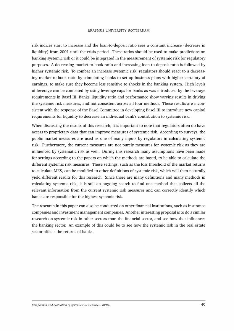
ERASMUS UNIVERSITY ROTTERDAM
risk indices start to increase and the loan-to-deposit ratio sees a constant increase (decrease in
liquidity) from 2001 until the crisis period. These ratios should be used to make predictions on
banking systemic risk or it could be integrated in the measurement of systemic risk for regulatory
purposes. A decreasing market-to-book ratio and increasing loan-to-deposit ratio is followed by
higher systemic risk. To combat an increase systemic risk, regulators should react to a decreas-
ing market-to-book ratio by stimulating banks to set up business plans with higher certainty of
earnings, to make sure they become less sensitive to shocks in the banking system. High levels
of leverage can be combated by using leverage caps for banks as was introduced by the leverage
requirements in Basel III. Banks’ liquidity ratio and performance show varying results in driving
the systemic risk measures, and not consistent across all four methods. These results are incon-
sistent with the response of the Basel Committee in developing Basel III to introduce new capital
requirements for liquidity to decrease an individual bank’s contribution to systemic risk.
When discussing the results of this research, it is important to note that regulators often do have
access to proprietary data that can improve measures of systemic risk. According to surveys, the
public market measures are used as one of many inputs by regulators in calculating systemic
risk. Furthermore, the current measures are not purely measures for systemic risk as they are
influenced by systematic risk as well. During this research many assumptions have been made
for settings according to the papers on which the methods are based, to be able to calculate the
different systemic risk measures. These settings, such as the loss threshold of the market returns
to calculate MES, can be modified to other definitions of systemic risk, which will then naturally
yield different results for this research. Since there are many definitions and many methods in
calculating systemic risk, it is still an ongoing search to find one method that collects all the
relevant information from the current systemic risk measures and can correctly identify which
banks are responsible for the highest systemic risk.
The research in this paper can also be conducted on other financial institutions, such as insurance
companies and investment management companies. Another interesting proposal is to do a similar
research on systemic risk in other sectors than the financial sector, and see how that influences
the banking sector. An example of this could be to see how the systemic risk in the real estate
sector affects the returns of banks.
Comparison and evaluation of systemic risk measures - KPMG 49

References
Acharya, V., R. Engle, and M. Richardson (2012). Capital shortfall: A new approach to ranking
and regulating systemic risks. The American Economic Review 102(3), 59–64.
Acharya, V., L. P. T. Philippon, and M. Richardson (2010). Measuring systemic risk. FRB of Cleveland
Working Paper 10(2).
Acharya, V., M. Richardson, S. van Nieuwerburgh, and L. White (2011). Guaranteed to fail: Fannie
mae, freddie mac, and the debacle of mortgage finance. Princeton University Press.
Acharya, V. and T. Yorulmazer (2003). Information contagion and inter-bank correlation in a
theory of systemic risk. CEPR Discussion Paper 3743.
Adrian, T. and M. Brunnermeier (2011). CoVaR. NBER Working Paper 17454.
Alessi, L. and C. Detken (2009). ’Real Time’ early warning indicators for costly asset price boom/-
bust cycles: A role for global liquidity. ECB Working Paper 1039.
Alfaro, R. and M. Drehmann (2009). Macro stress tests and crises: What can we learn? BIS
Quarterly Review.
Allen, F. and D. Gale (2000). Financial contagion. The Journal of Political Economy 108(1), 1–33.
Benoit, S., G. Colletaz, C. Hurlin, and C. Pérignon (2013). A theoretical and empirical comparison
of systemic risk measures. HEC Paris Research Paper 2014-1030.
Bertrand, M., E. Duflo, and S. Mullainathan (2004). How much should we trust differences-in-
differences estimates. Quarterly Journal of Economics 119(1), 249–275.
Billio, M., M. Getmansky, A. Lo, and L. Pelizzon (2011). Econometric measures of connectedness
and systemic risk in the finance and insurance sectors. Journal of Financial Economics 104,
535–559.
Bisias, D., M. Flood, A. Lo, and S. Valavanis (2012). A survey of systemic risk analytics. U.S.
Department of Treasury, Office of Financial Research 1.
Black, L., R. Correa, X. Huang, and H. Zhou (2015). The systemic risk of European banks during
the financial and sovereign debt crises. Journal of Banking & Finance 63, 107–125.
Borio, C. and M. Drehmann (2009). Assessing the risk of banking crises - revisited. BIS Quarterly
Review.
Brownlees, C. and R. Engle (2012). Volatility, correlation and tails for systemic risk measurement.
Available at SSRN 1611229.
Brunnermeier, M., A. Crockett, C. Goodhart, A. Persaud, and H. Shin (2009). The fundamental
principles of financial regulation. London: Centre for Economic Policy Research 11.
Comparison and evaluation of systemic risk measures - KPMG 50

ERASMUS UNIVERSITY ROTTERDAM
Bühler, W. and M. Prokopczuk (2010). Systemic risk: Is the banking sector special? Available at
SSRN 1612683.
Bullard, J., C. Neely, and D. Wheelock (2009). Systemic risk and the financial crisis. Federal
Reserve Bank of St. Louis Review 91(5), 403–418.
Capuano, C. (2009). The option-ipod: The probability of default implied by option prices based
on entropy. IMF Working Paper 8/194.
Chan, N., M. Getmansky, S. Haas, and A. Lo (2005). Systemic risk and hedge funds. National
Bureau of Economic Research 11200.
Chan-Lau, J., M. Espinosa, K. Giesecke, and J. Sole (2009). Assessing the systemic implications
of financial linkages. IMF Global Financial Stability Report 2.
Chen, H., J. Cummins, K. Viswanathan, and M. Weiss (2014). Systemic risk and the intercon-
nectedness between banks and insurers: An econometric analysis. Journal of Risk and Insur-
ance 81(3), 623–652.
Cummins, J. and M. Weiss (2014). Systemic risk and the U.S. insurance sector. Journal of Risk
and Insurance 81(3), 489–528.
de Bandt, O. and P. Hartmann (2000). Systemic risk: A survey. ECB Working Paper 35.
Driscoll, J. and A. Kraay (1998). How much should we trust differences-in-differences estimates.
The review of economics and statistics 80(4), 549–560.
Duffie, D. (2011). Systemic risk exposures: A 10-by-10-by-10 approach. NBER Working Pa-
per 17281.
Engle, R. (2002). Dynamic conditional correlation - a simple class of multivariate garch models.
Journal of Business & Economic Statistics 20(3), 339–350.
Gai, P. and S. Kapadia (2010). Contagion in financial networks. Proceedings of the Royal Society
of London A: Mathematical, Physical and Engineering Sciences.
Gavin, M. and R. Hausmann (1996). The roots of banking crises: The macroeconomic context.
IDB Working Paper 262.
Georg, C. and J. Poschmann (2010). Systemic risk in a network model of interbank markets with
central bank activity. Jena economic research papers 033.
Giesecke, K. and B. Kim (2011). Systemic risk: What defaults are telling us. Management Sci-
ence 57(8), 1387–1405.
Giglio, S., B. Kelly, and S. Pruitt (2016). Systemic risk and the macroeconomy: An empirical
evaluation. Journal of Financial Economics 119(3), 457–471.
Comparison and evaluation of systemic risk measures - KPMG 51

ERASMUS UNIVERSITY ROTTERDAM
Gray, D. and A. Jobst (2010). Systemic cca-a model approach to systemic risk. Deutsche Bun-
desbank/Technische Universität Dresden Conference: Beyond the Financial Crisis: Systemic Risk,
Spillovers and Regulation.
Huang, X., H. Zhou, and H. Zhu (2009). A framework for assessing the systemic risk of major
financial institutions. Journal of Banking & Finance 33(11), 2036–2049.
Huang, X., H. Zhou, and H. Zhu (2011). Systemic risk contributions. Finance and Economics
Discussions Series 8.
Huang, X., H. Zhou, and H. Zhu (2012). Assessing the systemic risk of a heterogeneous portfolio
of banks during the recent financial crisis. Journal of Financial Stability 8(3), 193–205.
IMF, BIS, FSB (2009). Guidance to assess the systemic importance of financial institutions, markets
and instruments: Initial considerations - background paper. Report to the G-20 Finance Ministers
and Central Bank Governors.
Kaufman, G. (2000). Banking and currency crisis and systemic risk: A taxonomy and review.
Financial Markets, Institutions & Instruments 9(2), 69–131.
Kaufman, G. and K. Scott (2003). What is systemic risk, and do bank regulators retard or con-
tribute to it? Independent Review.
Kupiec, P. and D. Nickerson (2004). Assessing systemic risk exposure from banks and gses un-
der alternative approaches to capital regulation. The Journal of Real Estate Finance and Eco-
nomics 28(2), 123–145.
Lagunoff, R. and S. Schreft (2001). A model of financial fragility. Journal of Economic Theory 99(1),
220–264.
Laina, P., J. Nyholm, and P. Sarlin (2015). Leading indicators of systemic banking crises: Finland
in a panel of eu countries. Review of Financial Economics 24, 18–35.
Lehar, A. (2005). Measuring systemic risk: A risk management approach. Journal of Banking &
Finance 29(10), 2577–2603.
Mundy, C. (2000). The nature of risk: The nature of systemic risk - trying to achieve a definition.
The Journal of Risk Finance 12(5), 29–31.
Newey, W. and K. West (1987). A simple, positive semi-definite, heteroskedasticity and autocor-
relationconsistent covariance matrix. Econometrica 55(3), 703–708.
Schwarcz, S. (2008). Systemic risk. Georgetown Law Journal 97(1).
Segoviano, M. and C. Goodhart (2009). Banking stability measures. Financial Markets Group,
London School of Economics and Political Science 627.
Comparison and evaluation of systemic risk measures - KPMG 52

ERASMUS UNIVERSITY ROTTERDAM
Shapley, L. (1953). Stochastic games. Proceedings of the National Academy of Sciences in the United
States of America 39(10), 1095–1100.
Tarashev, N., C. Borio, and K. Tsatsaronis (2010). Attributing systemic risk to individual institu-
tions. BIS Working Paper 308.
Tarashev, N. and H. Zhu (2008). Specification and calibration errors in measures of portfolio
credit risk: The case of the asrf model. International Journal of Central Banking 4(2), 129–173.
Varotto, S. and L. Zhao (2014). Systemic risk and bank size. Available at SSRN 2320693.
Comparison and evaluation of systemic risk measures - KPMG 53

ERASMUS UNIVERSITY ROTTERDAM
Appendix
A Literature review - systemic risk
Types of systemic risk
In academic literature, often the distinction within systemic events is made between an event
in a ‘narrow’ and a ‘broad’ sense (de Bandt and Hartmann, 2000). Systemic risk in the narrow
sense as an event is similar to contagion and can be seen as the release of negative news about a
financial institution or its default, or the crash of a financial market leading to considerable adverse
effects on one or several other financial institutions or markets. The broad sense of systemic risk
is traditionally seen as macroeconomic risks, such as common shocks or recessions. This means
that the trigger of the event could be a shock from outside or from within the financial system.
Systemic risk is largely categorized in three sources: contagion, common shocks and informational
spillovers (Kaufman, 2000).
Contagion effects in the ‘narrow’ sense emerge when firms within a system are interconnected
and have economic exposure to each other. Allen and Gale (2000) find that interconnectedness
in interbank markets leads to a better allocation of risk-sharing and liquidity allocation. They find
that especially in a complete interbank market, where each node is connected to every other node,
initial idiosyncratic shocks can be absorbed. On the other hand, they find that when the network
is incomplete, contagion effects will occur more strictly. This is consistent with Gai and Kapadia
(2010), who find that increased interconnectedness and risk-sharing leads to a lower probability of
contagious default. However, conditional on the failure of one firm triggering contagious defaults,
high interconnectedness increases the chance of contagion spreading more widely. An example
of systemic risk as cause of this contagion is a bank run (Mundy, 2004). In a bank run, many
depositors of a financial institution withdraw their cash at the same time, because of insecurity
about the institution’s solvency. This increases the chances of default for the financial institution
as they become unable to satisfy these withdrawals. The banking sector is very interconnected
thrugh interbank deposits, loans and clearings (Kaufman, 2000). One failure therefore causes
other banks or financial institutions to default as a consequence.
Another type of systemic risk are common shocks, which arises from indirect connections between
firms. Common shocks can be seen as systemic risk in the ’broad’ sense, focusing on contagion
from an initially exogenous external shock. This risk depends on correlation between firms rather
than direct causation. Systemic risk is then present when there are strong similarities between
firms’ risk exposures (Kaufman and Scott, 2003). Especially in the banking system, banks may
strategically choose to invest in similar assets as a reaction to negative externalities. Effects of the
2008 financial crisis were stronger due to the fact that many financial institutions had invested
in similar assets (subprime mortgages), exposing them to risk from a common shock. Georg and
Comparison and evaluation of systemic risk measures - KPMG 54

ERASMUS UNIVERSITY ROTTERDAM
Poschmann (2010) find that common shocks carry a greater threat to the stability of a system than
contagion effects.
Another source of systemic risk is informational contagion, also known as information spillovers.
Acharya and Yorulmazer (2003) suggest that this is an important type of systemic risk that should
also be taken into account. To illustrate information spillover effects, we consider two banks in
a banking system. If one bank fails to pay its depositors their interest, it gives a bad sign of the
overall state of the economy. Depositors of the other bank then quickly update their rates and
require a higher interest rate on their deposits. If both banks show good performance, then it is
taken as good news about the state of the economy, which is why depositors are willing to lend to
banks at lower interest rates. This implies that the borrowing cost of banks are lower if both banks
survive together than when one fails. This is an example of information spillover of one bank’s
failure on the other bank’s borrowing cost. An information contagion then follows if the surviv-
ing bank cannot afford the revised borrowing rate and fails as well. The greater the correlation
between loan returns of banks, the higher the chance that these banks will survive together. To
increase this interbank correlation, banks tend to lend to similar industries, which is also referred
to as bank herding. Intuitively, banks prefer to survive together, rather than surviving individually
as they want to avoid information spillover risk. The overall concept of information spillovers is
based on the fact that the insolvency of one bank can lead to an increase in refinancing cost of the
surviving banks. The financial crisis has made clear that banks show herding behavior (Acharya
and Yorulmazer, 2003). The authors show that banks attempt to counter this information conta-
gion risk by herding ex-ante and undertaking correlated investments to increase the likelihood of
joint survival.
Systemic risk in the financial sector
The term systemic risk is mostly used to denote the risk of a collapse of an entire financial system.
However, systemic risk is not a unique concept for only the financial sector. A default of a large
retailer for example, may have severe consequences to the firm’s suppliers and the local economy.
The recent bankruptcy of V&D in the Netherlands is an example for this, as the default of this
department store chain led to serious damage to their suppliers. Still, the failure of a nonfinancial
firm rarely leads to a threat to a competitor or the entire economic system. Compared to other
sectors, the financial system especially is vulnerable to systemic risk. For this reason, there is a
returning discussion on government regulation and supervision for large financial institutions to
reduce the negative consequences of systemic risk. Schwarcz (2008) argues that the financial
sector is vulnerable to systemic risk, because of the fact that financial institutions are important
sources of capital. Their failures can therefore lead to a decreased availability of capital in society,
especially when there are failures in a large number of institutions, and an increase of the cost of
capital. These are serious consequences that result from systemic failure. Gavin and Hausmann
Comparison and evaluation of systemic risk measures - KPMG 55

ERASMUS UNIVERSITY ROTTERDAM
(1996) mention several reasons why the banking system is more vulnerable than other industries.
Bullard et al. (2009) summarize three reasons, which fall in line with Gavin and Hausmann, why
especially the financial system contains systemic risks that other sectors do not hold.
The first reason is the interconnectedness of the financial sector. The banking sector is highly
interconnected due to bilateral transactions and relationships, such as interbank loans, trades
and other transactions. A big danger for financial institutions is settlement risk, which is the risk
that one party fails defaults on the terms of a contract with another party at the settlement date,
especially since financial institutions have large daily exposures that run into the billions in dollars.
It is difficult for a bank to have a clear overview of its counterparties, because of the lightning-
fast speed in which banks and market makers trade and the complexity of banks’ balance sheets
and securities. Therefore, a default of a large financial institution may lead to enormous losses
for other counterparty firms, as well as third parties that are again connected with these firms.
Lagunoff and Schreft (2001) construct a game theory model for what they refer to as financial
fragility. The model incorporates interrelated portfolios and payment commitments between firms
as linkages of financial institutions. They show that indeed an economy becomes more fragile and
a financial crisis occurs as defaults spread across the system, causing links to break.
Another reason why systemic risk is more of an issue for the financial sector than other sectors
is the leverage of financial institutions. As financial institution have a higher debt-to-equity ratio
compared to firms in other sectors, their return on equity will have a higher rate in good times,
but also a higher risk of default when the markets are turning against them. Because of this,
financial institutions as well as non-financial firms have the incentive to identify an optimal debt-
to-equity ratio. Compared to other sectors, financial firms have a significantly higher leverage
ratio, meaning that they fund their assets with debt rather than equity. The average leverage ratio
of financial institutions is 15.85 to 1 compared to 2.83 to 1 in the second highest leveraged sector,
services (as of April 2016). When there is a small drop in value of a highly leveraged institution,
it may have a severe effect on its equity, causing the firm to raise additional capital or sell their
assets. During the financial crisis, large investment banks such as Fannie Mae and Freddie Mac
had financial difficulties because of their high leverage (Acharya et al., 2011).
The third and last reason mentioned by Bullard et al. (2009) for why the financial sector is more
vulnerable to systemic risk than other sectors is the fact that financial firms tend to deal with
their holding of long-term assets with short-term liabilities. This mismatch of maturities in their
assets and liabilities makes financial institutions exposed to interest rate risks and liquidity shocks.
Financial intermediaries generally employ a gap strategy, where they borrow short and lend long.
This strategy is profitable as short rates are commonly lower than long rates. This can have adverse
effects as commercial banks rely on demand deposits, which means that depositors can withdraw
their funds at any time. If depositors suddenly decide to take out their funds because of times of
uncertainty, the bank can be forced into bankruptcy.
Comparison and evaluation of systemic risk measures - KPMG 56

ERASMUS UNIVERSITY ROTTERDAM
Also within the financial sector, different industry groups, such as banks, real estate, diversified
financials and insurance companies, have varying vulnerability to systemic risk. An empirical com-
parison of the degree of systemic risk across various sectors is conducted by Bühler and Prokopczuk
(2010). They find a significantly larger systemic risk in banks than in all other industries of the
economy. Billio et al. (2011) find an asymmetry in the degree of interconnectedness among vari-
ous financial industries. They show that banks and insurance companies have a larger impact on
hedge funds, brokers and dealers than the other way around, suggesting that banks and insurance
companies carry more systemic risk. They explain the asymmetry of the banks carrying more sys-
temic risk by the fact that banks lend capital to the other financial institutions. Chen et al. (2014)
examine the interconnectedness between banks and insurance companies using Granger causality
tests. They find that the impact banks have on insurance companies is stronger and of longer dura-
tion than vice versa. Furthermore they find that banks carry significant systemic risk for insurers
but not the other way around. Cummins and Weiss (2014) evaluate U.S. insurance companies
on their systemic risk and did not find significant results, implying that the default of insurance
companies will generally not cause significant systemic risk events affecting the economy.
Other systemic risk approaches
Macroeconomic measures for systemic risk lean on the aggregate imbalances in cases of financial
instability in the system. These imbalances are then seen as leading indicators for systemic risks.
Therefore, macroeconomic time series and statistics are used for systemic risk measures. For
example, Alessi and Detken (2009) test macroeconomic variables as early warning indicators for
costly aggregate asset price boom/bust cycles. In the same trend, Borio and Drehmann (2009)
look for simultaneous financial imbalances in equity prices, property prices and credit gaps as
indicators.
Another way to look at quantifying system risk in a financial system is to focus on the financial
sector as a whole instead of individual contributions of institutions (Giesecke and Kim, 2011).
One way to do this is by using a network model. In this framework, nodes represent legal entities
and edges stand for contractual financial agreements between them. For this network to repre-
sent the financial system, the contracts can be seen as cash-flow obligations where the contractual
relationships show the interconnectedness of the system. Using the network approach to assess
financial linkages was first proposed by Chan-Lau et al. (2009) in the IMF Global Financial Stabil-
ity Review, for which they primarily use institutional data to look at network externalities. Their
network model can track the consequences of a credit event or liquidity squeeze throughout the
entire system. Similarly, Tarashev et al. (2010) use the Shapley Value for risk allocation (Shapley,
1953) in a game theory network model to give a measure for institution’s risk contribution as well
as systemic-wide risk. Billio et al. (2010) use stock market data to create estimates of a latent
network structure for different industries within the financial sector: banks, brokers, hedge funds
Comparison and evaluation of systemic risk measures - KPMG 57

ERASMUS UNIVERSITY ROTTERDAM
and insurance companies. They use Granger-causality tests to identify the network of statistically
significant Granger-causal relations among these institutions. The drawbacks of a network ap-
proach is that it requires data on the exposures between financial institutions. Many studies have
tried to model the interconnections within the system without directly observing these exposures.
Chan-Lau et al. (2009) proposed the default intensity model, using default data, which captures
effects of direct and indirect linkages among financial institutions. This method then provides a
risk metric of potential failures due to these linkages.
Forward-looking risk measures have the goal of capturing the implied cash-flows of each of the
financial institutions for each contract that they hold. They can be useful for regulators in stress
testing financial institutions. To calculate these measures, (forward-looking) asset prices are used,
since movements in these prices reflect the changes in market anticipation on the future perfor-
mance of their underlyings (Huang et al., 2009). An example of this is the application of the
Contingent Claims Analysis (CCA), also known as the Merton (1973) model, to measure systemic
risk (Lehar, 2005; Gray and Jobst, 2010). Here, the contribution of each financial institution to
the total liability of the regulator is measured, using the Merton model for bank liabilities. Ca-
puano (2008) proposes a framework, using option prices, to derive the probability of default of
financial institutions. He then extends this framework to detect early signals for systemic risk.
Finally, Segoviano and Goodhart (2009) use CDS prices to see how individual institutions add to
the potential distress of the system.
Another forward-looking approach to look at systemic risk is stress testing. This is a form of
scenario-analysis, where the stability of the financial system is tested under possible, but extreme
circumstances. Stress testing is often used in regulation and standards, such as the European
Banking Authority or in Basel III, to calculate regulatory capital requirements for financial insti-
tutions. An example of a stress testing model for systemic risk is the macroeconomic stress test by
Alfaro and Drehmann (2009). They use an auto-regressive model of GDP growth as they assume
that typically the GDP growth decreases prior to crisis periods. Another approach is the 10-by-10-
by-10 approach by Duffie (2011), where he tests ten systemically important financial institutions
in different scenarios, such as the default of one of the institutions.
Comparison and evaluation of systemic risk measures - KPMG 58

Tabl
e8
(a)
Ban
kin
form
atio
nan
dch
arac
teri
stic
s
Ban
kna
me
Cou
ntry
Tota
lass
ets
Ran
kLe
vera
geR
ank
M/B
Ran
kLi
quid
ity
Ran
kPr
ofita
bilit
yR
ank
G-S
IBC
DS
Ran
k
AB
NA
MR
ON
VN
E74
1,60
213
9.21
331.
6914
145.
5253
0.12
44A
geas
BE
373,
269
245.
8570
1.22
4314
6.00
520.
1342
149.
6326
Alli
ance
&Le
ices
ter
PLC
GB
80,3
8453
8.28
412.
068
156.
2044
0.33
1211
9.53
34A
llied
Iris
hB
anks
PLC
IR12
6,08
443
17.5
010
1.98
914
7.64
51-0
.18
8375
0.52
6A
lman
ijN
VB
E24
0,41
029
10.9
623
0.58
8511
1.26
729.
851
Alp
haB
ank
AE
GR
53,8
0358
11.2
022
1.55
2414
9.17
500.
0464
985.
533
Ban
caA
nton
vene
taSp
AIT
46,2
0464
6.63
591.
4133
209.
1922
-0.0
579
172.
9121
Ban
caC
arig
eSp
AIT
30,2
5175
8.04
441.
1358
171.
2435
0.00
75B
anca
Lom
bard
aE
Piem
onte
seIT
35,5
6271
5.01
761.
4232
195.
3724
0.14
40B
anca
Mon
teD
eiPa
schi
DiS
iena
IT18
2,15
937
15.0
013
0.83
7119
1.75
25-0
.02
77B
anca
Naz
iona
leD
elLa
voro
IT83
,338
518.
1442
1.24
4121
0.29
210.
0466
37.0
751
Ban
caPo
polD
ell’E
mili
aR
omag
naIT
52,4
5960
8.87
370.
7379
156.
4943
0.10
49B
anca
Popo
lare
DiL
odiS
pAIT
42,9
3067
10.1
626
0.93
6623
6.96
18-0
.04
78B
anca
Popo
lare
DiM
ilano
IT44
,738
6510
.88
240.
7080
155.
4645
0.04
6324
8.55
14B
anca
Popo
lare
DiS
ondr
ioIT
24,3
2679
4.02
801.
2245
123.
2770
0.16
33B
anco
Bilb
aoVi
zcay
aA
rgen
taSP
459,
762
205.
2474
1.63
2013
8.33
590.
1925
Yes
53.9
948
Ban
coC
omer
cial
Port
ugue
sSA
PO80
,498
5211
.54
211.
1357
162.
4539
0.04
65B
anco
De
Saba
dell
SASP
92,3
5048
6.57
611.
2242
160.
4940
0.14
3919
6.43
16B
anco
Espi
rito
Sant
oSA
PO63
,656
549.
0235
1.05
6116
7.07
360.
0273
81.5
142
Ban
coPa
stor
SASP
22,1
8481
6.53
621.
5326
155.
2146
0.15
3712
4.19
29B
anco
Popo
lare
Soci
eta
Coo
pera
tiva
IT97
,522
4616
.23
120.
8669
198.
8523
0.07
55B
anco
Popu
lar
Espa
nolS
ASP
101,
220
456.
6758
1.65
1817
1.38
340.
1926
356.
839
Ban
coPo
rtug
ues
deIn
vest
imen
toSA
PO36
,727
708.
1143
1.22
4614
3.95
560.
1146
68.1
546
Ban
coSa
ntan
der
SASP
891,
133
105.
6273
1.21
4814
3.98
550.
1730
Yes
179.
1817
Ban
kO
fG
reec
eG
R55
,127
5717
.35
111.
5327
1,14
1.33
2-0
.69
86B
ank
Of
Irel
and
IR13
1,97
641
12.3
318
1.52
2815
0.19
490.
2120
113.
4035
Ban
kia
SASP
249,
067
289.
4229
1.02
6313
9.82
570.
0754
Ban
kint
erSP
42,7
9568
7.26
531.
8312
215.
1420
0.13
4329
2.06
11B
anqu
eC
anto
nale
Vaud
oise
SZ26
,466
774.
4078
1.62
2113
6.41
600.
2617
Comparison and evaluation of systemic risk measures - KPMG 59

Tabl
e8
(b)
Ban
kin
form
atio
nan
dch
arac
teri
stic
s
Ban
kna
me
Cou
ntry
Tota
lass
ets
Ran
kLe
vera
geR
ank
M/B
Ran
kLi
quid
ity
Ran
kPr
ofita
bilit
yR
ank
G-S
IBC
DS
Ran
k
Bar
clay
sPl
cG
B1,
380,
452
612
.60
161.
1455
134.
1563
0.18
28Ye
s12
2.27
30B
NP
Pari
bas
FR1,
699,
803
16.
2563
0.92
6710
3.97
740.
1050
Yes
36.7
652
Bra
dfor
d&
Bin
gley
PLC
GB
53,7
8459
21.5
99
1.45
301,
724.
201
0.26
1616
6.71
23C
aiss
eR
egio
nale
deC
r.Agr
.FR
28,3
3576
9.14
340.
7478
245.
3015
0.44
8C
aixa
bank
SASP
195,
638
334.
2679
0.82
7413
3.32
640.
447
Cap
ital
iaSp
AIT
131,
520
428.
2940
1.33
3619
1.27
260.
1341
24.3
154
Com
mer
zban
kA
GG
E59
2,59
816
31.7
15
0.61
8218
0.39
310.
0074
Yes
49.3
449
Cre
dit
Agr
icol
eSA
FR1,
455,
346
414
.76
150.
6084
123.
5169
0.02
72Ye
s13
1.03
28C
redi
tSu
isse
Gro
upA
GSZ
768,
570
129.
3631
1.14
5690
.71
830.
0561
Yes
101.
1539
Cre
dita
nsal
tA
S17
2,69
739
6.05
671.
6716
185.
4329
0.26
18C
redi
toVa
ltel
lines
eSc
arl
IT20
,717
828.
7238
0.61
8315
3.15
470.
0270
Dan
ske
Ban
kA
SD
E38
4,83
023
14.7
914
1.17
5223
7.67
170.
0853
120.
7233
Dep
faB
ank
PLC
IR18
6,89
735
38.2
23
2.06
792
1.95
40.
0658
860.
684
Deu
tsch
eB
ank
AG
GE
1,50
5,88
03
12.1
819
0.80
7572
.70
860.
0368
Yes
111.
0636
Deu
tsch
ePo
stba
nkA
GG
E18
6,06
836
9.42
301.
2739
102.
5376
0.04
62D
exia
SAB
E45
0,38
121
465.
711
0.86
7030
3.83
110.
0271
Yes
341.
4910
DN
BA
SAN
O18
9,33
434
7.78
491.
2147
182.
0930
0.20
2360
.22
47Em
pori
kiB
ank
Of
Gre
ece
SAG
R23
,302
806.
1265
2.42
212
4.30
68-0
.36
84Er
ste
Gro
upB
ank
AG
AS
175,
628
387.
8547
0.82
7312
4.36
670.
0659
178.
4119
Euro
bank
Erga
sias
SAG
R59
,531
5623
.55
61.
5525
135.
1262
8.47
299
5.09
2G
AM
Hol
ding
AG
SZ10
,679
851.
2986
1.84
1196
1.56
34.
883
Glit
nir
EHF
IC14
,927
836.
0369
2.31
334
5.51
80.
3810
367.
298
HB
OS
PLC
GB
707,
693
147.
7848
1.61
2217
4.25
330.
2022
71.2
245
HSB
CH
oldi
ngs
PLC
GB
1,67
5,77
32
2.76
831.
3037
99.2
479
0.25
19Ye
s83
.53
41H
ypov
erei
nsba
nkA
GG
E51
9,28
117
23.4
37
1.00
6523
1.17
19-0
.01
76IK
BD
euts
che
Indu
stri
eban
kA
GG
E38
,442
6944
.59
21.
0264
689.
185
-0.0
980
204.
4715
ING
Gro
epN
VN
E1,
082,
024
76.
1066
1.15
5412
1.86
710.
1048
Yes
27.7
553
Inte
saSa
npao
loSp
AIT
493,
799
186.
5860
0.91
6818
7.18
280.
1047
176.
2720
Inve
stec
PLC
SA43
,883
663.
4881
1.19
5012
4.80
660.
3213
Comparison and evaluation of systemic risk measures - KPMG 60
Tabl
e8
(c)
Ban
kin
form
atio
nan
dch
arac
teri
stic
s
Ban
kna
me
Cou
ntry
Tota
lass
ets
Ran
kLe
vera
geR
ank
M/B
Ran
kLi
quid
ity
Ran
kPr
ofita
bilit
yR
ank
G-S
IBC
DS
Ran
k
Iris
hB
ank
Res
olut
ion
Cor
pora
tion
IR49
,244
624.
9477
2.49
115
9.24
420.
494
822.
845
Juliu
sB
aer
Gro
upLt
dSZ
46,3
5363
2.15
841.
7813
75.9
785
0.27
14Jy
ske
Ban
kD
E31
,907
747.
0856
1.25
4015
9.84
410.
1732
Kau
pthi
ngB
ank
EHF
IC32
,396
735.
1475
2.09
634
0.58
90.
466
281.
0012
KB
CG
roep
NV
BE
299,
489
276.
0468
1.09
5910
2.05
770.
0852
75.6
243
Kom
ercn
iBan
kaA
SC
Z24
,949
781.
4085
2.15
598
.64
800.
465
Land
sban
kiH
FIC
14,6
8384
5.85
711.
9610
245.
0716
0.41
925
6.88
13Ll
oyds
Ban
king
Gro
upPL
CG
B83
1,33
711
7.08
571.
4331
145.
2254
0.17
31Ye
s14
7.56
27M
arfin
Inve
stm
ent
Gro
upH
oldi
ngs
GR
4,61
786
6.21
641.
0860
98.5
581
-0.6
785
Med
ioba
nca
SpA
IT62
,426
557.
2454
1.19
5159
3.07
60.
2021
172.
9022
Nat
iona
lBan
kO
fG
reec
eG
R90
,733
497.
6950
1.20
4910
3.47
75-0
.11
8110
21.3
11
Nat
ixis
Ban
ques
Popu
lair
esFR
385,
520
2221
.96
80.
7577
299.
9612
0.07
56Ye
s15
8.90
25N
orde
aB
ank
AB
SW46
7,60
719
7.14
551.
3735
163.
7838
0.14
38Ye
s84
.54
40N
RA
MPL
CG
B87
,850
5010
.54
252.
194
323.
8610
0.27
15O
PFi
nanc
ialG
roup
FI32
,505
729.
5727
1.30
3837
7.86
70.
1924
Pira
eus
Ban
kSA
GR
50,3
1661
12.4
017
1.16
5313
5.46
61-0
.17
8251
1.09
7R
aiff
eise
nB
ank
Inte
rnat
iona
lAG
AS
96,7
1647
7.30
521.
2244
139.
6358
0.19
27R
oyal
Ban
kO
fSc
otla
ndG
roup
GB
1,43
6,30
55
9.21
320.
8372
128.
1365
0.02
69Ye
s16
3.60
24Sa
npao
loIM
ISp
AIT
225,
990
305.
6372
1.67
1517
6.30
320.
1534
Sant
ande
rU
KPL
CG
B31
9,92
125
33.8
54
0.24
8610
9.44
730.
1829
179.
1817
Skan
dina
visk
aEn
skild
aB
anke
nA
BSW
221,
699
317.
6651
1.40
3416
4.37
370.
1245
105.
1838
Soci
ete
Gen
eral
eSA
FR1,
026,
358
98.
4739
0.80
7698
.27
820.
0657
Yes
46.7
050
Stan
dard
Cha
rter
edPL
CG
B30
3,64
226
3.25
821.
5923
99.9
178
0.35
11Ye
s12
2.17
31Sv
ensk
aH
ande
lsba
nken
AB
SW21
9,19
932
9.50
281.
6617
266.
4513
0.15
3572
.56
44Sw
edba
nkA
BSW
168,
409
407.
9046
1.47
2926
3.19
140.
1536
121.
2232
Ubi
Ban
caSp
AIT
108,
431
4412
.12
200.
6781
188.
4827
0.03
67U
BS
Gro
upA
GSZ
1,08
1,38
08
7.99
451.
6319
77.8
284
0.05
60Ye
s11
0.92
37U
nicr
edit
SpA
IT67
9,85
515
8.97
361.
0362
151.
9348
0.09
51Ye
s
Not
eTh
ista
ble
disp
lays
the
the
bank
char
acte
rist
ics
for
each
ofth
e86
Euro
pean
bank
sta
ken
asan
aver
age
ofqu
arte
rly
data
acro
ssth
efu
llsa
mpl
epe
riod
Janu
ary
2001
toD
ecem
ber
2015
.B
ecau
seof
avai
labi
lity,
the
data
for
the
liqui
dity
rati
o,w
hich
isth
elo
an-t
o-de
posi
tra
tio,
isin
year
lyfr
eque
ncy.
Furt
herm
ore
the
CD
Ssp
read
data
isin
daily
freq
uenc
yan
dis
only
show
nfo
rth
e56
bank
s,fo
rw
hich
CD
Sda
tais
avai
labl
ein
Dat
astr
eam
.Th
eto
tala
sset
sar
ein€
m.
The
leve
rage
rati
ois
calc
ulat
edas
(boo
kva
lue
ofde
bt+
mar
ket
valu
eof
equi
ty)
divi
ded
byth
em
arke
tva
lue
ofeq
uity
.M
arke
t-to
-boo
kis
the
rati
oof
mar
ket
equi
tyva
lue
over
the
book
equi
tyva
lue.
Toas
sess
liqui
dity
,the
loan
-to-
depo
sit
rati
ois
take
n,w
hich
isth
eto
tall
oans
divi
ded
byth
eto
tald
epos
its
ofa
bank
.Fi
nally
,the
profi
tabi
lity
isde
fined
asth
ere
turn
onas
sets
,whi
chis
the
net
inco
me
divi
ded
byth
eav
erag
eto
tala
sset
sas
ape
rcen
tage
.Th
eta
ble
furt
her
show
sho
wea
chba
nkra
nks
inea
chba
nkch
arac
teri
stic
sepa
rate
ly.
Fina
lly,t
heta
ble
show
sw
heth
erth
eba
nkis
cons
ider
eda
Glo
balS
yste
mic
ally
Impo
rtan
tB
ank
(G-S
IB)
byth
eFS
B.T
heda
tais
take
nfr
omD
atas
trea
m.
Comparison and evaluation of systemic risk measures - KPMG 61

ERASMUS UNIVERSITY ROTTERDAM
B Driscoll and Kraay standard errors
Consider the within-transformed fixed effects regression model:
y∗i t = β′X ∗i t + ε
∗i t i = 1, ..., N , t = 1, ...T
where yi t is the dependent variable, X i t a K × 1 vector of dependent variables, The observations
across firms are stacked as one variable for the panel model as follows:
yi t = (y1t11, y1t12
, ..., y1T1, y2t21
, ..., yN TN)′
X = (x1t11, x1t12
, ..., x1T1, x2t21
, ..., xN TN)′
which means that the panel data is allowed to be unbalanced. The error terms εi t can be het-
eroskedastic, autocorrelated and correlated in the cross-section. Then the parameter β is consis-
tently estimated by OLS as β = (X ′X )−1X ′ y .
The Driscoll and Kraay covariance matrix is as follows:
V (β) = (X ′X )−1ST (X′X )−1 (30)
of which the square roots of the diagonal terms are the robust standard errors. Here the ST is
defined by Newey and West (1987) as:
ST = Ω0 +m(T )∑
j=1
w( j, m)(Ω j + Ω′j) (31)
Here m(T ) is the number of lags up to which the errors may be autocorrelated. For simplicity, we
take m(T ) = floor(4(T/100)2/9) following Newey and West (1994), which is a rule of thumb, but
not necessarily optimal. The so-called Bartlett weights make sure that ST is positive semi-definite
and that high order lags are assigned lower weights:
w( j, m(T )) = 1− j/(m(T ) + 1) (32)
The K × K matrix Ω j is defined as
Ω j =T∑
t= j+1
ht(θ )ht− j(θ )′ with ht(θ ) =
N(t)∑
i=1
hi t(θ ) (33)
where in case of panel OLS estimation, the hi t(θ ) is a vector of moment conditions of the linear
Comparison and evaluation of systemic risk measures - KPMG 62

ERASMUS UNIVERSITY ROTTERDAM
regression model as shown
hi t(θ ) = x i t εi t = x i t(yi t − x ′i t θ ) (34)
C PCA
2005 2007 2010 2012 2015
z-s
core
-3
-2
-1
0
1
2
3
4
5
6
7
8
First PC
Figure 10: First component PCA systemic risk measuresThis figure shows the first principal component, which accounts for the largest variance over the foursystemic risk measures, MES, ∆CoVaR, SRISK and DIP from January 1st, 2004 until December 31st, 2015.The principal component is reported as z-scores, which means the number of standard deviations awayfrom the historical mean taken over the complete time sample. The vertical dashed lines indicate majorevents in the crises periods. (1) September 15th, 2008: Lehman Brothers bankruptcy. (2) May 2nd, 2010:Greek government bailout (3) November 30th, 2011: Federal Reserve, ECB and European central bankslower dollar swaps.
Comparison and evaluation of systemic risk measures - KPMG 63

ERASMUS UNIVERSITY ROTTERDAM
D Systemic risk ranking
Table 9 Systemic risk rankings
Ranking MES ∆CoVaR SRISK DIP
1 Bank Of Ireland UBS Deutsche Bank BNP Paribas2 Allied Irish Banks ING BNP Paribas Deutsche Bank3 Credit Agricole Credit Suisse Credit Agricole HSBC4 Marfin Investment Group Unicredit ING Barclays5 Societe Generale Erste Group Bank Societe Generale Royal Bank of Scotland6 Banco Santander Banco Bilbao Viz.Arg. Commerzbank Credit Agricole7 Emporiki Bank Of Greece Deutsche Bank Unicredit ING8 Ageas Banco Santander Banco Santander Banco Santander9 Banco Bilbao Viz.Arg. Skandinaviska Enskilda Dexia Lloyds Banking Group
10 ING Nordea Bank UBS Societe Generale11 Mediobanca DNB Intesa Sanpaolo UBS12 Banca Popol Di Milano Raiffeisen Bank Intl. Credit Suisse Unicredit13 National Bank Of Greece Caixabank Natixis Banques Popul. Credit Suisse14 Lloyds Banking Group Swedbank Banco Bilbao Viz.Arg. Commerzbank15 BNP Paribas Jyske Bank KBC Groep Intesa Sanpaolo16 Raiffeisen Bank Intl Ubi Banca Banca Monte Dei P.S. Dexia17 Natixis Banques Popul. KBC Group Deutsche Postbank Nordea Bank18 Bankinter Svenska Handelsbanken Bank Of Ireland Banco Bilbao Viz.Arg.19 Banco Espirito Santo Banco Portugues Invest. Allied Irish Banks Natixis Banques Popul.20 Dexia Commerzbank Banco Popol. Soc.Coop. Danske Bank
Note This table shows the top 20 systemic risk rankings for each of the systemic risk measures MES,∆CoVaR, SRISK and DIP at December31st, 2010. A total of 86 European banks are considered.
Comparison and evaluation of systemic risk measures - KPMG 64