msxr209 residentialschool booklet - · pdf filetma01, andthe comments that...
TRANSCRIPT

Mathematics and Computing/Science/TechnologyMSXR209 Mathematical modelling
MSXR209 RSB
MSXR209Residential School Booklet
Copyright c© 2008 The Open University SUP 87036 4
2.2

The Open University, Walton Hall, Milton Keynes, MK7 6AA.
First published 2005. Second edition 2006.
Copyright c© 2006, 2008 The Open University
Edited, designed and typeset by The Open University, using the Open University TEX System.
Printed and bound in the United Kingdom by Thanet Press Ltd, Margate.
SUP 87036 4
2.2
Contents
Introduction 4
1 Mathematical modelling sessions 41.1 Exploring the problem 4
1.2 Formulating and evaluating the model 51.3 Writing the report 6
1.4 A sample report 7
2 Group activity sessions 72.1 Air track session 8
2.2 V-scope session 12
2.3 Data analysis session 162.4 Sensitivity analysis session 27
3 Exercises on mathematical methods 303.1 Classification of differential equations 30
3.2 First-order differential equations 31
3.3 Linear constant-coefficient differential equations 333.4 Gaussian elimination 36
3.5 Determinants 383.6 Eigenvalues and eigenvectors 38
3.7 Systems of linear differential equations 41
3.8 Partial derivatives 44
4 Exercises on mechanics 45
4.1 Forces 45
4.2 Static objects 474.3 One-dimensional motion 48
4.4 Oscillations 514.5 Conservation of energy 52
4.6 Projectiles 53
4.7 Damping, forcing and resonance 544.8 Normal modes 58
Appendix: Sample report for TMA 02 62
Solutions to the exercises 73

Section 1 Mathematical modelling sessions
IntroductionThe Course Guide informed you of the various teaching components of theresidential school, and of how they relate to each other and to the assessmentof the course. This booklet contains information about, and guidance on,the work that you will be doing at residential school.
This booklet may seem daunting at first, but note that not everything in itneeds to be read or studied. Sections 1 and 2 give details about the workthat you will be doing during the week, whereas Sections 3 and 4 are to helpyou to revise any topics with which you feel unfamiliar, and which you mayneed for one of the group activities.
Section 1 is really a reinforcement of the input to be provided by the tutorat the mathematical modelling sessions, which are based around TMA 02.
Section 2 gives detailed information about the group activity sessions. You The timetable given to you atthe beginning of the week willdetail the order in which youare to tackle these sessions.
should read the Safety information, Aims and Prerequisite knowledge beforeyou undertake each particular activity, since they give guidance on how toprepare for the session and on the mathematical techniques that you willneed for that session. If you wish to refresh your understanding of some ofthese techniques, then you can use Section 3 or 4.
Section 3 (mathematical methods) and Section 4 (mechanics) contain a largenumber of exercises divided into topics. For several topics there is a starterquestion, to help you to decide whether you should do some further exerciseson this topic. There will be revision sessions during the week, and you canseek help from your fellow students or from the tutors.
1 Mathematical modelling sessionsTMA 02 asks you to undertake a modelling exercise based on your choiceof one of three problems. While you are at residential school you will spenda fair amount of time working on your problem, in a group with fellow Working in a group can be
stimulating and very helpful.By bouncing ideas off eachother, listening and debating,more progress is made thanwould be done in isolation.
students and with guidance from a tutor. When you return from residentialschool you should extend and complete your work on the problem, and thenwrite up your results in the form of a report. This report forms the wholeof TMA 02.
If you work effectively while you are at residential school, you should havea well-developed model by the time you return home. You will then needto check your results, compare your predictions with reality, criticize andrevise your model, before writing your report.
1.1 Exploring the problem
A mathematical model is a set of relations between variables representingthe main features of the situation being modelled. Before one can begin toformulate a model, it is necessary to obtain a feel for the problem. This maybe difficult if one is dealing with a situation that is at all complicated or un-familiar. This subsection describes a technique for starting on a modellingproblem that many people find helpful. The technique uses ‘brainstorming’to produce a list of features of the situation. Then, using this feature list,one can usually see how to select some appropriate variables and begin to
4

Section 1 Mathematical modelling sessions
obtain an idea of how they might be related. The technique relates to twoimportant modelling skills:• identifying the important features of a problem;• deciding which of these features should be included in a first, very simple,
model.
The suggested technique is as follows.
(a) List as many features as you can which have something to do with theproblem. This is the ‘brainstorming’ part of the activity. You shouldnot pause to analyse the features as you write them down, but simplyaim to generate a stream of ideas. As a result, your list may includesuperficial and even irrelevant ideas; but write them down anyway, be-cause sometimes something that is superficial or irrelevant may lead youto think of another more important feature.
(b) Refine this list by omitting everything except the features that are rel-evant and ‘sensible’. Then try to link together those of the remainingfeatures that influence each other. In contrast to the previous step, thisis a reflective and analytical process.
(c) Prune the refined feature list, so as to leave only a very few featuresthat you regard as absolutely essential. Your aim is to identify just twoor three key variables that will appear in your model. It will probablybe necessary to be quite ruthless with this pruning. In deciding whichfeatures to keep and which to discard, you will have to make simplifyingassumptions: for example, you may decide that one feature has a farmore significant effect than another on the process under consideration.Remember that, if you are going to represent a feature in your modelby a variable, you must be able to quantify it. While carrying out thispruning, you should bear in mind that modelling proceeds by stages:your first model should be as simple as possible, but it may form thebasis for further models, which will be better and more complex. Theassumptions made in pruning your feature list, and the features thatyou decide to omit at this stage, will be useful later when you come tocriticize and to improve your first model — so keep a note of them.
At residential school you will use this technique while working in a group The groups will be arrangedso that all students in a groupare working on the samemodelling problem.
under the guidance of a tutor, so you will be able to pool your ideas withthose of other students.
1.2 Formulating and evaluating the model
By the end of your residential school week, you should at least have devel-oped a first model to the point where you can see how to provide an answerto the problem posed; the residential school programme has been organizedto ensure this. Since your work will be supported by a tutor, there is noneed to go into detail here about how to do the modelling; besides, the pro-cesses involved have been discussed at some length in the Introduction tomathematical modelling .
After you return from residential school, it should not take long to obtain asolution to the original problem, if you did not quite reach this stage whileat residential school. However, this is not the end of the modelling process.It is important to evaluate your results and also the model that producedthem. You will want to assess how accurate and reliable your results are.For this purpose, a data sheet is provided at residential school, which may beof use in evaluating your model. It is sometimes difficult to predict what data
5
Section 1 Mathematical modelling sessions
are needed, and the data provided may not be what you require; so you mayneed to collect alternative data about the situation you are modelling, eitherby consulting books, searching on the internet, or possibly by carrying out asimple experiment or engaging in some other form of observation. However,please do not ask institutions to provide you with data, unless it is publiclyavailable. Remember that many other students are engaged in the sameactivity as yourself; imagine the effect if they all wrote simultaneously tothe same body, asking for information.
You will be very fortunate if the results from your first model prove to be en-tirely satisfactory when compared with reality, since your first model shouldhave been a simple one. You will therefore need to revise and improve yourmodel, which involves another circuit of the modelling cycle. One goodmethod of finding a way to revise your model is to review the simplifyingassumptions that you made when formulating it. Take each of the simpli-fying assumptions in turn, and try to work out the effect on your model ofremoving or relaxing it. Alternatively, you could try to incorporate one ofthe features that you eliminated when pruning your feature list. The revi-sion to the model should be based on a reason why it would improve themodel; there is no point in including a revision for its own sake.
When you have decided how to revise your model, you should carry out the However, you are notexpected to solve themathematics for your revisedmodel.
necessary modifications to the formulation of the model.
1.3 Writing the report
Your purpose, when you come to write the report on your modelling exercise,is to explain to your tutor what results you obtained and how you obtainedthem, and to do this clearly and fully, so that he or she will be left in nodoubt about what you have achieved. After all, your tutor cannot awardmarks for work that he or she does not understand, nor can your tutor beexpected to guess what you did if you have not written it down. It is yourresponsibility to explain your work satisfactorily.
TMA 02 is similar to other TMAs in this respect. The difference is thatsolutions for other TMAs mostly follow a fairly straightforward pattern thatis dictated by the questions. In the case of TMA 02, however, you apparentlyhave a great deal of freedom in the way that you organize your report andin your choice of words and symbols. The purpose of this subsection is togive you some advice about how to write your report. Further advice is contained in
TMA 02 itself, which includesthe mark scheme. See alsothe sample report referred toin Subsection 1.4.
You do not need to aspire to exacting standards of literary style. Your tutorwill not worry unduly about occasional spelling mistakes. On the otherhand, you should be concerned with those aspects of writing that are closestto mathematics: being systematic; laying out your work in a logical fashion;making sure that each step of an argument or calculation follows from theprevious one; avoiding any obscurity or ambiguity in the use of symbols andtechnical terms; using appropriate diagrams and tables. Moreover, no pieceof writing is going to make much sense if it contains lots of meaninglessor ambiguous sentences, so you should also ensure that what you write isclearly expressed.
Your report will actually be read (and marked) by your tutor, of course; but,in writing your report, you may find it helpful to imagine that it is to beread by another student. This should allow you to make sensible judgementsabout the amount of mathematical detail to include.
6

Section 2 Group activity sessions
Although your report should have the structure described in the mark This structure is followed inthe sample report referred toin Subsection 1.4.
scheme for TMA 02, this does not mean that it must be written in theorder in which it will be finally presented and read. Most people find itquite difficult to write anything longer than a postcard by starting at thebeginning and keeping steadily on until the end is reached. It is usuallynecessary to make at least one rough draft, and to work backwards and A word processor can be very
useful in producing a reportin this way.
forwards through the draft as the ideas develop. If you proceed in this way,you will find that the resulting account of your model is more comprehensiveand better structured than if you just start at the beginning and carry onto the end.
Take every opportunity to include figures and illustrations in your report.You can give sketches of graphs, drawings of experimental equipment, anddiagrams of processes and relationships. You can also include output fromMathcad. Explanations of complicated derivations are often easier to un-derstand if they are accompanied by appropriate diagrams. Data, numericalresults and even lists of variables are usually best displayed in tables.
You may find it helpful during your latter work on TMA 02 to find one The comments that youreceive on your work onTMA 01, and the commentsthat you write to others in thepeer-marking session, shouldhelp you with TMA 02.
or two (non-mathematical) friends who might be interested in the problemthat you are going to solve. Persuade them to be your audience and askthem to read your report when first drafted. Your audience will be usefulfor discussion when you become stuck, and should help you to produce areport that is clear and easy to understand.
1.4 A sample report
To give you some idea of what a report written with the suggested structurelooks like, there is a sample report in the Appendix. This demonstrates howto use a mixture of text, mathematics, Mathcad, graphs and tables. Thereport addresses the problem described below.
Problem addressed in sample reportThe most common form of central heating uses radiators to heat up therooms of a house. Suppose that you are thinking of installing or replacingthe radiators in your house. What size and how many radiators should youinstall in each room? Larger radiators cost more but tend to heat up theroom more quickly. The cost of buying and installing radiators is a one-offcost, whereas the cost of the energy needed to use the radiators is ongoing.Is it important to try to minimize costs or is it more important to reducethe time for the room to warm up?
Construct a mathematical model that will enable you to make a sensiblechoice as to how best to install new radiators.
2 Group activity sessionsThere are four group activity sessions in which you will engage during theweek, working in small groups. At the end of the week, your group will give The allocation of presentation
topics will be decided towardsthe end of the week.
a presentation of the work that you have done in one of these sessions.
Each session has an associated subsection below. This includes a list of themathematical techniques that are required for that session.
7

Section 2 Group activity sessions
Two of the sessions are based on modelling with mechanics; there are fourpurposes to these sessions. The first purpose is to give you more experiencein mathematical modelling. The second purpose is to give you practice insetting up equations of motion, solving them and interpreting the results.The third purpose is for you to find out how good the simplifying modellingassumptions really are. The final purpose is to give you a practical feel forthe objects that are modelled as particles, model springs, model pulleys, etc;handling these objects will be of help to you in analysing their motion andbehaviour.
The topics in the two ‘modelling with mechanics’ sessions are: The order in which you dothe two sessions will dependon the arrangements for yourresidential school week.
• the vibrations of a system composed of masses and springs, leading topredictions for the periods of normal mode motions;
• the modelling assumptions of a constant coefficient of sliding friction andof a model pulley.
The suggested approach for both of the ‘modelling with mechanics’ sessionsis as follows:• handle the objects and the apparatus to obtain a feel for the forces
involved, to discover what forces act on the objects, to understand thepossible relationships and to view the possible motions;
• identify important variables, make simplifying assumptions and drawappropriate diagrams;
• decide which of the symbols defined are variables, and which are param-eters for which data values will be needed;
• obtain and then solve the equations of motion; At this stage the equationsshould contain algebraicsymbols, not numbers.You need to note carefully theunits of measurement; theymay not be SI units.
• decide on what measurements are needed, either to provide data for themodel or for validation of the model;
• perform the experiments that you have decided are necessary;• compare the results from the model with reality;• reconsider the assumptions and, if necessary, revise the model.
You should discuss the modelling, and the measurement of data, with thetutors as you go along. Note that it is better to do the modelling first, beforeyou make any measurements. It is only when you have a first model thatyou will know what you need to measure.
Details of the two ‘modelling with mechanics’ sessions are contained in Sub-sections 2.1 and 2.2.
2.1 Air track session
Safety informationIf handled with reasonable care, the apparatus is safe and should cause noproblems. It is best not to wear open-toed footwear for this session, in caseone of the masses falls off the table. If you are suspending a mass from aspring, make sure that the mass is firmly attached to the end of the spring.
AimsThe aims of this modelling session are:• to construct a model for the motion of one or two objects connected by
springs to two fixed points and moving along the line joining the twofixed points;
• to measure the appropriate parameters to evaluate the model;• to predict the motion of the objects under specified circumstances;• to compare the predictions with experimental outcomes.
8
Section 2 Group activity sessions
Prerequisite knowledgeFor this session, you will need an understanding of the following.
Topic Subsection in MST209this booklet unit
Model the forces due to springs 4.4, 4.8 7Set up an equation of motion 4.3 6Solve, and interpret, second-order linear constant-coefficient differential equations
3.3 3
Solve simultaneous second-order linear differentialequations
3.7 11
Normal mode motion 4.8 18
IntroductionThe objects are called gliders. They move over a track pierced with holesthrough which air is blown. The air comes from a blower attached to the air You may have observed
experiments with such an airtrack and gliders on thevideos associated withMST209 Units 6 and 19.
track by a hose pipe. The gliders are supported by the air, and their motionon the air track is almost frictionless. When you are familiarizing yourselfwith the motion of the gliders, you should convince yourself that they doindeed move with very little friction.
This session is in two parts, each to do with the motion of objects (gliders)attached to springs. The first part concerns a single glider; the second partinvolves two gliders.
Equipment listThe apparatus should contain at least the following:
• air track with blower• two gliders• three springs• spring balance• retort stand with clamp• wooden ruler
• hanger and weights• stopwatch• cleaning spray• paper towels• graph paper
Practical notes• The air track and gliders should be cleaned if you feel that they are
sticking. Use the cleaning spray and paper towels.• The air track should be level. To check that it is, put one of the gliders
in the middle of the air track and switch on the blower; the glider shouldstay in the middle or move very slowly. The air track can be levelled byturning the adjustment screws on its supporting legs.
• Please take great care of the surfaces of the air track and of the undersideof the gliders. Scratches on these surfaces may impair the frictionlessmotion of the gliders.
• The gliders should be moved on the air track only after the blower hasbeen switched on.
9

Section 2 Group activity sessions
Part I: A single object
Aim
The main aim of this part of the modelling session is to predict the period This activity is relevant toMST209 Unit 7 .of motion of the glider, and to compare your prediction with the measured
value. Your prediction will depend on the values of certain parameters ofthe system, and this activity will also help to validate the accuracy of thenumerical values that you find for these parameters. These parameter values will
also be useful in the secondpart of the session.Procedure
1. Arrange a system in which one of the gliders is connected by two springsto the two fixed ends.
2. Consider what forces act on the glider and on what those forces depend.3. Set up a model to predict the motion of the glider, using variables and
parameters for a general system of this type.4. Find an expression for the period of the motion in terms of the param-
eters associated with the system.5. Consider how you might find numerical values for the parameters of the
particular system with which you are working.6. Discuss with a tutor the work done so far. Explain what modelling
assumptions you have made, what your expression is for the period andyour suggestions on how to obtain the required data.
7. Set up experiments to find numerical values for the parameters, and thenan experiment to find the actual period of the system. How does yourobserved value for the period compare with your prediction? Does yourmodel require a revision?
Possible points to consider for the presentation
The three most important characteristics of a vibrating system are:• the period of the motion;• the amplitude of the motion;• the equilibrium position.
How do the following properties of the system with one glider and two springsaffect each of the characteristics above?• the stiffnesses of the springs;• the natural lengths of the springs;• the point at which the glider is released;• the distance between the fixed ends;• the mass of the glider.
10

Section 2 Group activity sessions
Part II: Two objects
Aim
The system is extended to two gliders and three springs. The aim of this This activity is relevant toMST209 Unit 18 .part of the modelling session is to predict both the periods and displacement
ratios for normal mode motions, so that (using the latter) you can measurethe periods of the normal modes.
Procedure
1. Connect the two gliders together by means of a spring, and connectthe other side of each glider to a fixed end with another spring. Then Try to arrange the gliders and
springs asymmetrically.obtain a feel for the motion by displacing one of the gliders along theline joining the two ends and watching the motion. How does it differfrom the motion of the system with only one glider?
2. Set up a model of the motion for the two gliders under the action of thethree springs, using variables and parameters to model a general systemof this type. Now that the system is more complicated, it is even moreimportant to define axes and variables. A diagram or two is essential.
3. Consider how you might find numerical values for the parameters. You Some of the measurementsthat you made for theone-glider system could beused here.
may also like to consider the following questions.• How important is it to know the equilibrium positions?• How does the motion depend on the initial displacements and veloc-
ities of the gliders?• How does the motion depend on the distance between the fixed ends?
4. Discuss with a tutor the work done so far. Explain what modellingassumptions you have made, what your equations of motion are, andyour suggestions on how to obtain the data.
5. Make the appropriate measurements to find parameter values, substitutethem into the equations of motion, and deduce the periods of the normalmodes of the system and the corresponding displacement ratios.
6. Use your predicted values for the displacement ratios to set up the nor-mal modes for the actual system, and confirm that the two gliders thenmove with the same frequency.
7. Compare the measured periods of the normal modes with the predictedvalues. Does your model require revision?
Possible points to consider for the presentation
The three most important characteristics of a vibrating system are:• the period of the motion;• the amplitude of the motion;• the equilibrium position.
How do the following properties of the system with two gliders and threesprings affect each of the characteristics above?• the stiffnesses of the springs;• the natural lengths of the springs;• the points at which the gliders are released;• the distance between the fixed ends;• the masses of the gliders.
In your presentation, you should give an account of what normal modemotion means.
11

Section 2 Group activity sessions
2.2 V-scope session
Safety informationIf handled with reasonable care, the apparatus is safe and should cause noproblems. Some of the suggested activities involve the motion of objects,whose mass is no more than 0.15 kg. It is important that the equipment isarranged so that, should the objects fall, they do not land on your toes. It isadvisable not to wear open-toed footwear during this session. The electronicsignals from the buttons are perfectly safe.
AimsThe aims of this modelling session are to determine whether two commonly This session is relevant to
MST209 Units 5 and 6 .used modelling assumptions in mechanics bear any resemblance to reality.These assumptions are:• a constant value for the coefficient of sliding friction;• no friction in a pulley (as assumed for a model pulley).
Prerequisite materialFor this session, you will need an understanding of the following.
Topic Subsection in MST209this booklet unit
Model the forces due to strings, normal reactions,friction
4.2 5, 6
Model a pulley 4.2 5Set up an equation of motion 4.3 6
IntroductionThe coefficient of sliding friction can be determined only when there is mo-tion. In the first part of this session, you are asked to set up an equation ofmotion and, by deducing an acceleration from measurements, to determinethe value of the friction coefficient.
For the second part, you will investigate the motion of two objects attachedto either end of a string that passes over a pulley, in order to test the as-sumption of a model pulley. It is possible to deduce the tensions in the stringon either side of the pulley by measuring the acceleration of the objects.
The third part involves motion with both a pulley and sliding friction. Hereyou can make assumptions that may have been modified by your observa-tions in the first two parts.
The motion of the objects can be measured by an instrument called theV-scope, whose operation is explained below.
Equipment listThe apparatus should contain at least the following.
• V-scope, microprocessor, PC• V-scope button• board, about 1.5 m long• block with a hook attached
• string• pulley• two hangers and weights• retort stand with clamp
12

Section 2 Group activity sessions
The V-scopeThe operation of the V-scope will be demonstrated in the introduction tothis session. The following is a synopsis of its operation.
The V-scope is a miniature global positioning system, with the ability tomeasure the positions of up to four small transponders, called buttons , in A transponder is a device
that sends out electronicsignals which can be pickedup by a receiver.
Because there are four(differently coloured) buttons,four different motions can betracked at one go. (Thesampling period increaseswith the number of buttons.)
three dimensions to an accuracy of 1mm, or better, at intervals of 10ms.Each lightweight button is attached to a point on the object whose position isto be measured. The V-scope provides data not only on the position of eachbutton at a given time, but also, for example, on the velocity, accelerationand linear momentum of a button. It is also possible to define one’s ownfunction and for the V-scope software to display values for it.
In more detail, the V-scope works as follows. The base stations, calledtowers , send out an infra-red signal that is picked up by the button, whichthen emits an ultrasonic signal. This ultrasonic signal is picked up by thetowers and the elapsed time of the signal is measured. The time takeninforms the microprocessor of the distance between the button and eachof the towers, and from this the (x, y, z) coordinates of the button can becalculated. The velocity and acceleration can be derived by considering the Derived variables, such as
speed, velocity andacceleration, are calculated bythe software from the positionmeasurements.
difference between adjacent positions at 10ms (0.01 s) intervals.
All the controls for recording the motion are on the PC screen. To beginrecording the position of one or more buttons, click on the red-coloured boxin the toolbar. After a period of initialization, a black tower symbol replacesthe normal mouse pointer symbol on the screen and the recording begins;the position of the button(s) is recorded by coloured dots on the graph. Tostop recording, press any key or click the mouse. To the right of the redrecording button are the symbols for restart, play, pause, step forward and The data can be trimmed, so
that only those for therelevant time interval areretained.
step backward, of the type often to be found on a video or DVD player. Theslider bar can be used to move the recording to any particular time.
To show a different graph, select the Display menu, and choose either New(to create an additional graph) or Edit (to modify the current graph). Fromthe first column of variables, choose one to be the independent variable, andfrom the second column choose the dependent variables. It is possible to display more
than one dependent variableat a time, but this can beconfusing. It is advisable touse only one or at most twodependent variables on anygiven graph.
Practical notes
• Each button must be within about 2.5 m of the towers and in a directline of sight, to receive the infra-red signal from the towers.
• When not in use the buttons should be kept away from direct light,preferably in a box.
• There may be interference from adjacent buttons. Buttons of the samecolour emit an ultrasonic signal of the same frequency. Choose coloursthat are different from those used by the groups nearby.
• To avoid spurious signals, it is best to orientate the layout of the appa-ratus so that direct sunlight does not fall on the face of any button.
• The special button mounts can be attached to any object whose positionis to be measured, by peeling off the adhesive seal and pressing theadhesive side of the mount onto a clean and flat surface.
• Be careful to look at the correct variables and to consider the scales onthe axes of graphs displayed on screen; not doing so is a common causeof experimental error when using the V-scope.
• When measuring acceleration with the V-scope, it is better to plot speedagainst time and to find the slope of the graph (the V-scope software canbe used to find the best-fit line) rather than to plot acceleration againsttime directly and to try to fit a constant to the data. In the former case,
13

Section 2 Group activity sessions
there is an averaging process, whereas in the latter, the extra calculationinvolved in finding the acceleration at individual points suffers more fromnoise in the original data.
Familiarization with the V-scopeBefore beginning your investigation, satisfy yourself that the V-scope isrecording the motion of a button, and that the axes are as labelled, bymoving the button vertically, and horizontally, both parallel and perpendic-ular to the plane of the towers.
For each partEach of the three parts of this session involves a system of one or moreobjects in motion. Once you have modelled the system, discuss with a tutorthe work done so far. Explain what modelling assumptions were made, whatyour equation of motion is, and your suggestions as to what data are needed.
After discussion with the tutor, make measurements not only to obtainvalues for the parameters but also for the evaluation of your model. If yourmodel is not adequate, consider which of the simplifying assumptions mayhave to be changed in order to improve the model.
Part I: Block sliding down a plane
Aim
The aim is to estimate the coefficient of sliding friction by inclining theboard and letting the block slide down it (see Figure 2.1).
Procedure
1. Draw a diagram showing all of the forces acting on the block.2. Write down the equation of motion for a particle sliding down a plane,
and use this to derive an expression for the coefficient of sliding friction.3. Now use the V-scope to make relevant measurements, and hence find
a value for the coefficient of sliding friction. (It is best to measure themotion side-on with the V-scope.)
4. Do the measurements confirm the simplifying assumption that the coef-ficient of sliding friction is independent of speed? Figure 2.1
Part II: Using a pulley
Aim
The aim is to investigate how well a real pulley is approximated by a modelpulley.
Procedure
1. Pass the string over the pulley, and attach objects of different masses(i.e. two hangers carrying different weights) at either end of the string(see Figure 2.2).
2. One object will descend while the other ascends, and the pulley willrotate. Model the motion of the two objects, and from this obtain ex-pressions for the tensions in the string on either side of the pulley. Figure 2.2
14
Section 2 Group activity sessions
3. Use the V-scope to obtain data on the motion. (It may be best to havethe towers on the floor and pointing upwards, to measure the verticalmotion, but make sure that the descending object does not hit the tow-ers. The button should be attached to the base of one of the hangers —preferably the one that ascends — and something soft should be placedon the floor so that the descending object can come to rest safely.)
4. From your analysis of the system and measurements, how well do youthink a real pulley is modelled by a model pulley?
5. If it is necessary to revise the assumptions about this pulley, formulatea new modelling assumption for it.
Part III: Moving a block on a plane by using a pulley
Aim
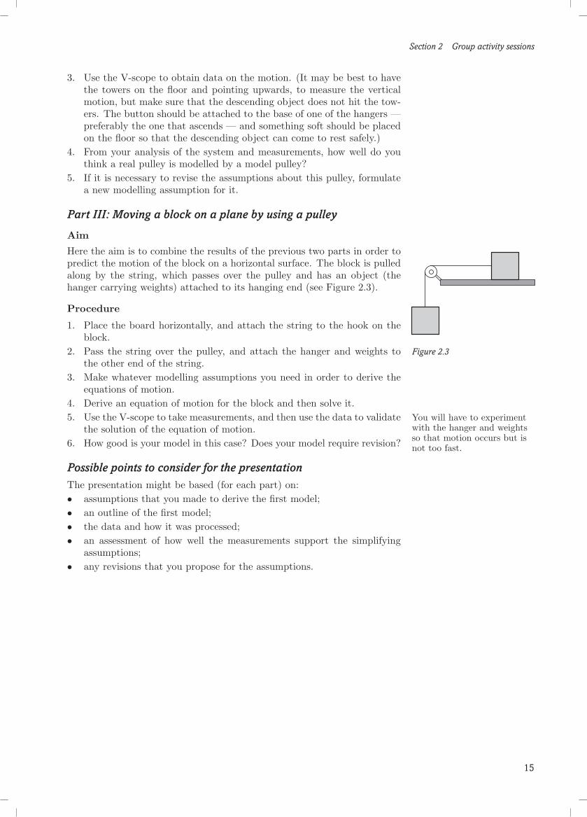
Here the aim is to combine the results of the previous two parts in order topredict the motion of the block on a horizontal surface. The block is pulledalong by the string, which passes over the pulley and has an object (thehanger carrying weights) attached to its hanging end (see Figure 2.3).
Procedure
1. Place the board horizontally, and attach the string to the hook on theblock.
2. Pass the string over the pulley, and attach the hanger and weights to Figure 2.3the other end of the string.
3. Make whatever modelling assumptions you need in order to derive theequations of motion.
4. Derive an equation of motion for the block and then solve it.5. Use the V-scope to take measurements, and then use the data to validate You will have to experiment
with the hanger and weightsso that motion occurs but isnot too fast.
the solution of the equation of motion.6. How good is your model in this case? Does your model require revision?
Possible points to consider for the presentationThe presentation might be based (for each part) on:• assumptions that you made to derive the first model;• an outline of the first model;• the data and how it was processed;• an assessment of how well the measurements support the simplifying
assumptions;• any revisions that you propose for the assumptions.
15
Section 2 Group activity sessions
2.3 Data analysis session
Safety informationThere is some data collection in this group activity, and most of it is nodifferent from performing some measurements in the home, of lengths, timesor temperatures.
One of the data collection activities involves using a special apparatus, witha heavy pendulum. For this, please ensure that the pendulum is releasedonly when the safety door is closed. Please do not open the door again untilthe pendulum is at rest. The pendulum motion can be brought to a halt byraising the lever on the left which acts as a brake on the pendulum.
Some data are to be collected using an ultrasound distance meter with alaser pointer. Before you use this, make sure that you know the direction inwhich the laser will point, and that no one is, or will be, in the line of thebeam.
AimsThe aims of this session are:• to understand what is meant by regression analysis;• to find the equation of best fit for data collected by the group;• to find a confidence or prediction interval for predicted values;• to improve your Mathcad skills.
Prerequisite knowledgeThe topic is introduced at residential school, but some familiarity with basic This familiarity could have
been obtained from MST121Block D.
statistical terminology is useful. You will also need to be able to use Mathcadworksheets.
IntroductionRegression analysis can be used to test whether there is a linear relationship Non-linear relationships can
often be transformed intolinear relationships.
between two variables, and to make predictions. This topic is introducedat residential school, and a summary of the main ideas and some examplesare included here, so that you have a model from which to work and anindication of how to use the Mathcad worksheet. You will collect your ownsets of data, analyse them and make some deductions from them.
Summary of regression analysis
Linear regression
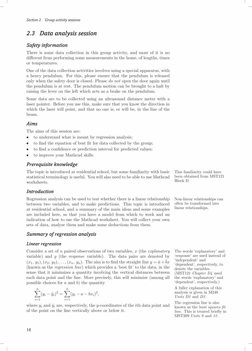
Consider a set of n paired observations of two variables, x (the explanatory The words ‘explanatory’ and‘response’ are used instead of‘independent’ and‘dependent’, respectively, todenote the variables.(MST121 Chapter D4 usedthe words ‘explanatory’ and‘dependent’, respectively.)A fuller explanation of thisanalysis is given in M248Units D2 and D3 .The regression line is alsoknown as the least squares fitline. This is treated briefly inMST209 Units 9 and 12 .
variable) and y (the response variable). The data pairs are denoted by(x1, y1), (x2, y2), . . . , (xn, yn). The aim is to find the straight line y = a + bx(known as the regression line) which provides a ‘best fit’ to the data, in thesense that it minimizes a quantity involving the vertical distances betweeneach data point and the line. More precisely, this will minimize (among allpossible choices for a and b) the quantity
n∑i=1
(yi − yi)2 =n∑
i=1
(yi − a− bxi)2,
where yi and yi are, respectively, the y-coordinates of the ith data point andof the point on the line vertically above or below it.
16
Section 2 Group activity sessions
Linear regression
For the set of data pairs (xi, yi) (i = 1, 2, . . . , n), the average values(means) of xi and yi are
x =1n
n∑i=1
xi, y =1n
n∑i=1
yi.
The sums of squares and products of deviations from the means are
Sxx =n∑
i=1
(xi − x)2 =( n∑
i=1
x2i
)− nx2, The calculations involved are
straightforward to performusing Mathcad.
Sxy (= Syx) =n∑
i=1
(xi − x)(yi − y) =( n∑
i=1
xiyi
)− nxy,
Syy =n∑
i=1
(yi − y)2 =( n∑
i=1
y2i
)− ny2.
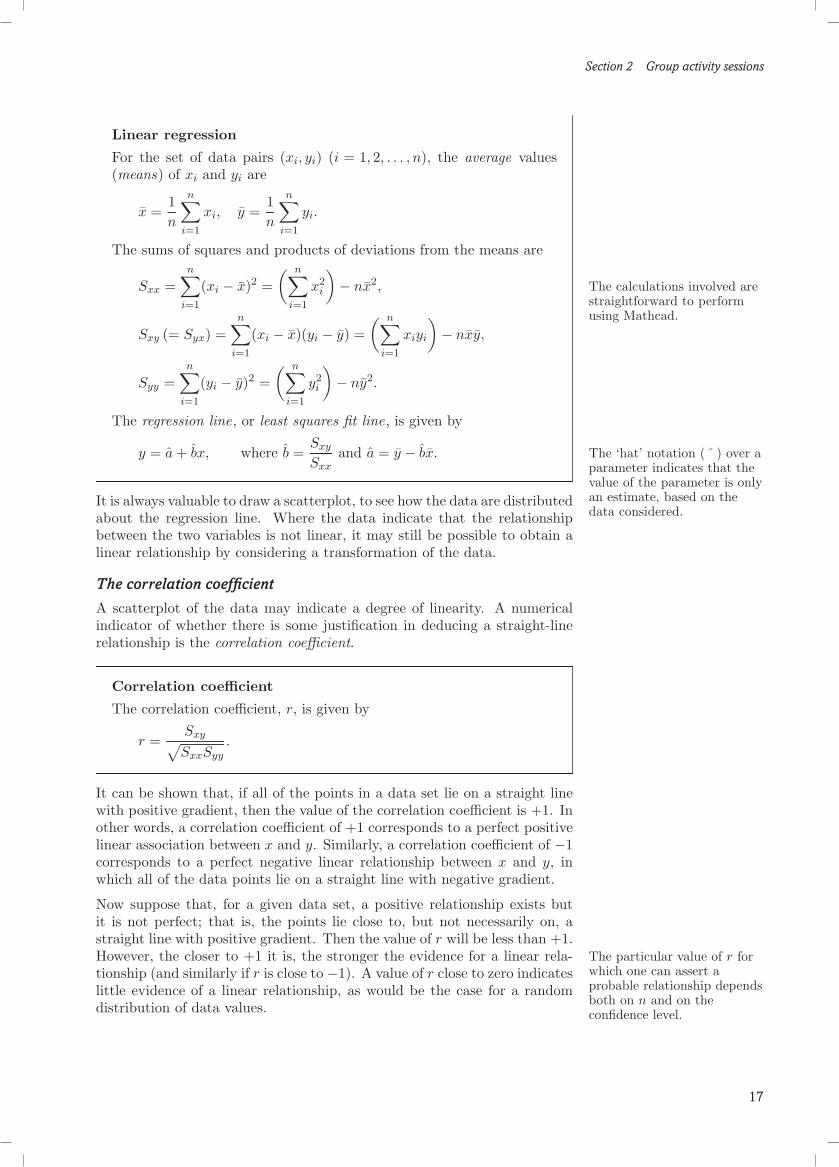
The regression line, or least squares fit line, is given by
y = a + bx, where b =Sxy
Sxxand a = y − bx. The ‘hat’ notation ( ˆ ) over a
parameter indicates that thevalue of the parameter is onlyan estimate, based on thedata considered.
It is always valuable to draw a scatterplot, to see how the data are distributedabout the regression line. Where the data indicate that the relationshipbetween the two variables is not linear, it may still be possible to obtain alinear relationship by considering a transformation of the data.
The correlation coefficient
A scatterplot of the data may indicate a degree of linearity. A numericalindicator of whether there is some justification in deducing a straight-linerelationship is the correlation coefficient.
Correlation coefficient
The correlation coefficient, r, is given by
r =Sxy√SxxSyy
.
It can be shown that, if all of the points in a data set lie on a straight linewith positive gradient, then the value of the correlation coefficient is +1. Inother words, a correlation coefficient of +1 corresponds to a perfect positivelinear association between x and y. Similarly, a correlation coefficient of −1corresponds to a perfect negative linear relationship between x and y, inwhich all of the data points lie on a straight line with negative gradient.
Now suppose that, for a given data set, a positive relationship exists butit is not perfect; that is, the points lie close to, but not necessarily on, astraight line with positive gradient. Then the value of r will be less than +1.However, the closer to +1 it is, the stronger the evidence for a linear rela- The particular value of r for
which one can assert aprobable relationship dependsboth on n and on theconfidence level.
tionship (and similarly if r is close to −1). A value of r close to zero indicateslittle evidence of a linear relationship, as would be the case for a randomdistribution of data values.
17

Section 2 Group activity sessions
Interval estimation
Linear regression assumes that the variables x and y are related by an equa-tion y = a + bx, where a, b have definite but unknown values, and wheremeasured values yi involve random fluctuations about a + bxi. The esti-mates a and b for the values of the parameters a and b, as found from aparticular sample (data set), will usually be different to those obtained fromanother sample, unless the samples are very large. Hence there is a measure The collection of data in large
samples may involve a lot ofwork, and one aim ofstatistical analysis is toestimate how good theparameter values are, evenwhen the number of datapoints is small.
of uncertainty in the values of these parameters. Based on one data sample(provided that more than two data pairs are measured), it is possible toestimate also an interval in which the values of the underlying parametersa and b are likely to lie. This process is called interval estimation.
Interval estimates
Suppose that a, b are estimates obtained from a single data set for theparameters a, b, where y = a + bx is the assumed linear model.
The corresponding confidence limits for b are given by
b± t
√Syy − S2
xy/Sxx
n− 21
Sxx(for n > 2). Here t is a parameter that
depends on the sample size nand on the confidence levelrequired (typically 95%or 99%). Some values of t,obtained from tables or froma Mathcad function, are asfollows in the second andthird columns.
Sample Confidencesize, n level
95% 99%
5 3.182 5.84110 2.306 3.35515 2.160 3.01225 2.069 2.807
100 1.984 2.627
The corresponding confidence limits for a are given by
a± t
√Syy − S2
xy/Sxx
n− 2
(1n
+x2
Sxx
)(for n > 2).
In each case, the interval between the two confidence limits is calledthe corresponding confidence interval .
The prediction limits for a single observation of y at x are given by
a + bx± t
√Syy − S2
xy/Sxx
n− 2
(1 +
1n
+(x− x)2
Sxx
)(for n > 2).
The interval between the two prediction limits is called the correspond-ing prediction interval .
A word is called for here about the difference between confidence and predic-tion limits (and the corresponding intervals). A confidence interval applieswhere the quantity to be estimated is assumed to have a definite (but un-known) value, as is the case for either of the parameters a and b. This alsoapplies for the mean value of all responses y, taken over a large number of The expressions for the
confidence limits for thismean value are as for theprediction limits given in thebox above, but with theremoval of the first term ‘1’from within the large bracket.Hence the prediction intervalfor a single observation (for agiven x and confidence level)is wider than thecorresponding confidenceinterval for the mean value ofmany such observations.
independent measurements, but all corresponding to one value of x.
However, the prediction of a single observation corresponding to a particularvalue of x carries a further level of uncertainty, since it is subject to randomfluctuation about the mean value just referred to. Hence the ‘95% confidenceinterval’ for a single observation is called a 95% prediction interval.
The meaning of the 95% confidence interval for b is that there is probability0.95 that the actual value of b lies within this interval (and similarly forconfidence intervals for other quantities and for other confidence levels).On the other hand, the meaning of the 95% prediction interval for a singleobservation of y (for a given value of x) is that there is probability 0.95 thatthe single observation will lie within this interval.
If the confidence interval for b includes zero, then it is possible that there isno relationship between the two variables. This is equivalent to the correla-tion coefficient not being (statistically) significantly different from zero.
18

Section 2 Group activity sessions
The prediction limits for a single observation can be used to estimate wherea subsequent data point associated with the variables x and y is likely to lie.These prediction limit expressions, viewed now as functions of x, can alsobe used to plot corresponding graphs above and below the regression line.
Examples
There follow three examples in which these ideas are put into practice, withreference to a Mathcad worksheet that you will be able to use for your owndata analysis.
Example 2.1
This example concerns the results of an investigation into whether measure-ments of the density of timber beams might be used to predict the strengthof the beams. Measuring the strength of timber is cumbersome and time-consuming, whereas density is much easier to measure. The table at right This is Data Set 1 on the
worksheet.
Density (x) Strength (y)
0.499 11.140.558 12.740.604 13.130.441 11.510.550 12.380.528 12.600.418 11.130.480 11.700.406 11.020.467 11.42
Source: M248 Unit D2 .
contains data for a sample of ten beams (in appropriate units).
(a) Draw a scatterplot of these data, using Mathcad. From this, determinewhether it is reasonable to propose a straight-line relationship betweenthe two variables.
(b) Find the equation of the regression line, and plot this line on the scat-terplot.
(c) Calculate the correlation coefficient. Do you consider that the strengthof timber beams can be estimated from measurements of their density?
(d) Use the equation of the regression line to estimate the strength of atimber beam whose density is 0.485.
(e) Use Mathcad to plot graphs of the 95% prediction limits, for all valuesof x within the data range, and find the 95% prediction interval for thestrength of a timber beam whose density is 0.485.
Solution
(a) The graph below displays a scatterplot of these data. All of the calculations aredisplayed in this solution.However, it suffices to use theMathcad worksheet to derivethe answers.
Figure 2.4 The data for timber density and strength
The data indicate that a linear relationship is a good model for the twovariables.
19

Section 2 Group activity sessions
(b) The relevant part of the output from the Mathcad worksheet is as fol- Mathcad cannot reproduce allof the symbols that are usedin the text. Hence, in theworksheet, ‘xbar’ stands for x,‘aest’ for a, and ‘arange’ for theconfidence limits for a, andsimilarly for y and b; ‘p’ is theconfidence level for theconfidence or predictionlimits, expressed as apercentage. Other symbolsare as in the text.
lows.
Figure 2.5 Summary statistics for the timber data
Hence the equation of the regression line is
y = 6.519 + 10.822x.
This line is displayed on the graph below, together with the original Note that one of the datapoints is some way from theregression line.
data points.
Figure 2.6 The timber data with regression line
The best estimate for the slope is 10.822, but there is some variability.The two entries in the Mathcad vector brange are the lower and upper95% confidence limits. The conclusion is that there is probability 0.95that the value of the slope lies between 6.887 and 14.757; this is quite awide range.
(c) The correlation coefficient is given (from Figure 2.5) by
r = 0.913.
This is fairly close to +1, suggesting strongly a positive linear rela-tionship. The conclusion is that the strength of timber beams can beestimated from measurements of their density.
(d) When x = 0.485, the estimated value of the corresponding strength is Beware of the dangers ofextrapolation, which is use ofthe regression line to predictvalues of the response variableoutside the range of valuesspanned by the explanatoryvariable. This should beavoided because there is noinformation on what happensoutside this range.
y = 6.519 + (10.822× 0.485) / 11.768.
20
Section 2 Group activity sessions
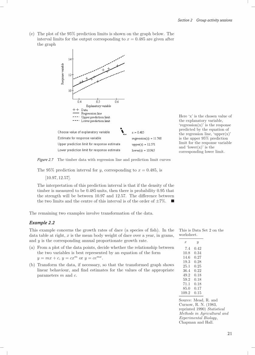
(e) The plot of the 95% prediction limits is shown on the graph below. Theinterval limits for the output corresponding to x = 0.485 are given afterthe graph.
Figure 2.7 The timber data with regression line and prediction limit curves
The 95% prediction interval for y, corresponding to x = 0.485, is
Here ‘x’ is the chosen value ofthe explanatory variable,‘regression(x)’ is the responsepredicted by the equation ofthe regression line, ‘upper(x)’is the upper 95% predictionlimit for the response variableand ‘lower(x)’ is thecorresponding lower limit.
[10.97, 12.57].
The interpretation of this prediction interval is that if the density of thetimber is measured to be 0.485 units, then there is probability 0.95 thatthe strength will be between 10.97 and 12.57. The difference betweenthe two limits and the centre of this interval is of the order of ±7%.
The remaining two examples involve transformation of the data.
Example 2.2
This example concerns the growth rates of dace (a species of fish). In the This is Data Set 2 on theworksheet.
x y
7.4 0.4210.8 0.3414.6 0.2719.3 0.2825.1 0.2536.4 0.2249.2 0.1859.2 0.1871.1 0.1885.0 0.17
109.2 0.15
Source: Mead, R. andCurnow, R. N. (1983,reprinted 1990) StatisticalMethods in Agricultural andExperimental Biology ,Chapman and Hall.
data table at right, x is the mean body weight of dace over a year, in grams,and y is the corresponding annual proportionate growth rate.
(a) From a plot of the data points, decide whether the relationship betweenthe two variables is best represented by an equation of the formy = mx + c, y = cxm or y = cemx.
(b) Transform the data, if necessary, so that the transformed graph showslinear behaviour, and find estimates for the values of the appropriateparameters m and c.
21

Section 2 Group activity sessions
Solution
(a) A plot of the data points is shown below.
Figure 2.8 Untransformed dace data
This does not appear linear. Using Mathcad, try both a log–log and alog–linear plot.
In Figure 2.9, the explanatoryvariable is lnx and theresponse variable is ln y. Ify = cxm, then thecorresponding relationship
ln y = ln c + m ln x
should show up as a straightline on this graph, with slopem = b and (ln y)-interceptln c = a.
In Figure 2.10, theexplanatory variable is x andthe response variable is ln y.If y = cemx, then thecorresponding relationship
ln y = ln c + mx
should show up as a straightline on this graph, with slopem = b and (ln y)-interceptln c = a.
Figure 2.9 Log–log plot for dace data
Figure 2.10 Log–linear plot for dace data
22
Section 2 Group activity sessions
From Figures 2.9 and 2.10, it looks as if the relationship is better rep-resented by y = cxm, since the log–log plot is closer to a straight linethan is the log–linear plot.
(b) The values of the parameters from the worksheet are as follows.
Figure 2.11 Summary statistics for log–log transformation of data
Fitting a regression line to the log–log plot gives b = −0.357 and
The value of the correlationcoefficient r is −0.984 for thetransformed data. This isclose to −1, indicating anegative linear relationshipbetween ln x and ln y.
a = −0.238. Hence the estimate for m is −0.357, and that for c isexp(−0.238) / 0.789. The equation of best fit is
y = 0.789x−0.357.
Example 2.3
In an experiment into the growth of duckweed, growth was monitored bycounting duckweed fronds at weekly intervals for eight weeks, starting oneweek after the introduction of a single duckweed plantlet (with 20 fronds)into water. The data are shown at right. This is Data Set 3 on the
worksheet.
Week (x) Fronds (y)
1 302 523 774 1355 2116 3267 5508 1052
Source: M248 Unit D2 .
(a) From a plot of the data points, decide whether the relationship betweenthe two variables is best represented by an equation of the formy = mx + c, y = cxm or y = cemx.
(b) Transform the data, if necessary, so that the transformed graph showslinear behaviour, and find estimates for the values of the appropriateparameters m and c.
(c) Find a 95% confidence interval for m.
Solution
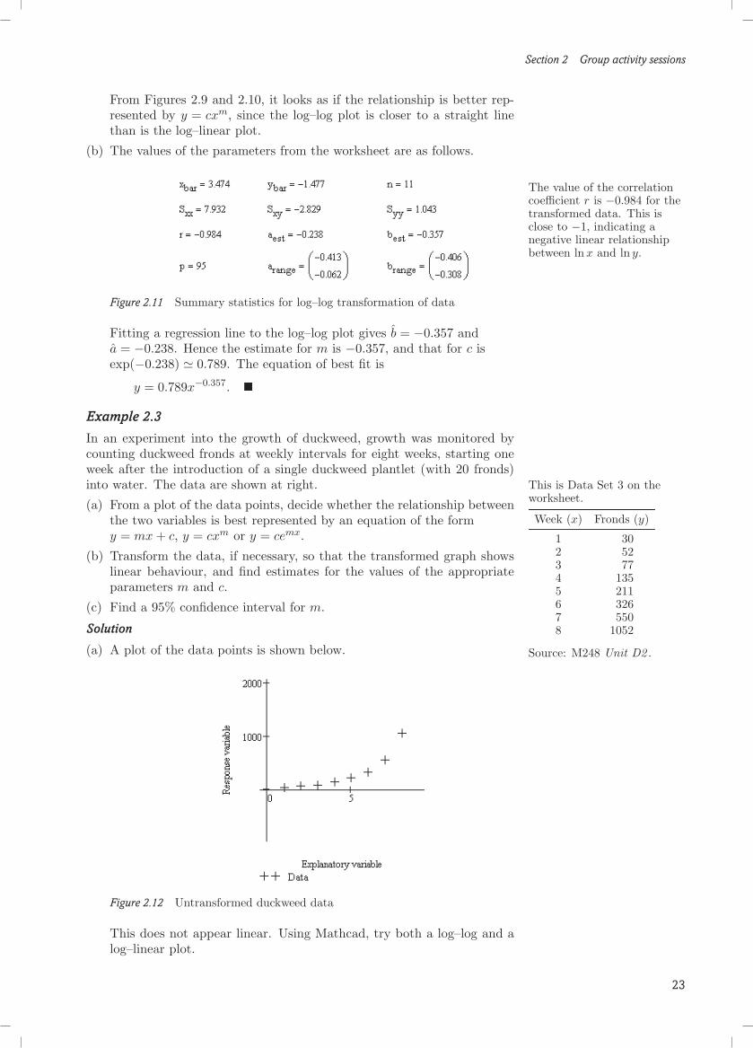
(a) A plot of the data points is shown below.
Figure 2.12 Untransformed duckweed data
This does not appear linear. Using Mathcad, try both a log–log and alog–linear plot.
23

Section 2 Group activity sessions
Figure 2.13 Log–log plot for duckweed data
Figure 2.14 Log–linear plot for duckweed data
From these two plots, it looks as if the relationship is better representedby y = cemx, since the log–linear plot is closer to a straight line than isthe log–log plot.
(b) The values of the parameters from the worksheet are as follows.
Figure 2.15 Summary statistics for log–linear transformation of duckweed data
Fitting a regression line to the log–linear plot gives b = 0.494 and
The value of r is 0.999 for thetransformed data. This isvery close to +1, indicatingstrongly a positive linearrelationship between xand ln y.
a = 2.904. Hence the estimate for m is 0.494, and the estimate forc is exp(2.904) / 18.256. The equation of best fit is
y = 18.256e0.494x.
(c) From Figure 2.15, a 95% confidence interval for the value of m is
[0.469, 0.519].
24
Section 2 Group activity sessions
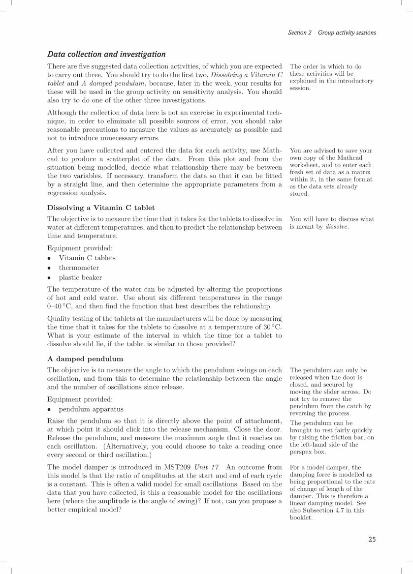
Data collection and investigationThere are five suggested data collection activities, of which you are expected The order in which to do
these activities will beexplained in the introductorysession.
to carry out three. You should try to do the first two, Dissolving a Vitamin Ctablet and A damped pendulum, because, later in the week, your results forthese will be used in the group activity on sensitivity analysis. You shouldalso try to do one of the other three investigations.
Although the collection of data here is not an exercise in experimental tech-nique, in order to eliminate all possible sources of error, you should takereasonable precautions to measure the values as accurately as possible andnot to introduce unnecessary errors.
After you have collected and entered the data for each activity, use Math- You are advised to save yourown copy of the Mathcadworksheet, and to enter eachfresh set of data as a matrixwithin it, in the same formatas the data sets alreadystored.
cad to produce a scatterplot of the data. From this plot and from thesituation being modelled, decide what relationship there may be betweenthe two variables. If necessary, transform the data so that it can be fittedby a straight line, and then determine the appropriate parameters from aregression analysis.
Dissolving a Vitamin C tablet
The objective is to measure the time that it takes for the tablets to dissolve in You will have to discuss whatis meant by dissolve.water at different temperatures, and then to predict the relationship between
time and temperature.
Equipment provided:• Vitamin C tablets• thermometer• plastic beaker
The temperature of the water can be adjusted by altering the proportionsof hot and cold water. Use about six different temperatures in the range0–40 ◦C, and then find the function that best describes the relationship.
Quality testing of the tablets at the manufacturers will be done by measuringthe time that it takes for the tablets to dissolve at a temperature of 30 ◦C.What is your estimate of the interval in which the time for a tablet todissolve should lie, if the tablet is similar to those provided?
A damped pendulum
The objective is to measure the angle to which the pendulum swings on each The pendulum can only bereleased when the door isclosed, and secured bymoving the slider across. Donot try to remove thependulum from the catch byreversing the process.The pendulum can bebrought to rest fairly quicklyby raising the friction bar, onthe left-hand side of theperspex box.
oscillation, and from this to determine the relationship between the angleand the number of oscillations since release.
Equipment provided:• pendulum apparatus
Raise the pendulum so that it is directly above the point of attachment,at which point it should click into the release mechanism. Close the door.Release the pendulum, and measure the maximum angle that it reaches oneach oscillation. (Alternatively, you could choose to take a reading onceevery second or third oscillation.)
The model damper is introduced in MST209 Unit 17 . An outcome from For a model damper, thedamping force is modelled asbeing proportional to the rateof change of length of thedamper. This is therefore alinear damping model. Seealso Subsection 4.7 in thisbooklet.
this model is that the ratio of amplitudes at the start and end of each cycleis a constant. This is often a valid model for small oscillations. Based on thedata that you have collected, is this a reasonable model for the oscillationshere (where the amplitude is the angle of swing)? If not, can you propose abetter empirical model?
25
Section 2 Group activity sessions
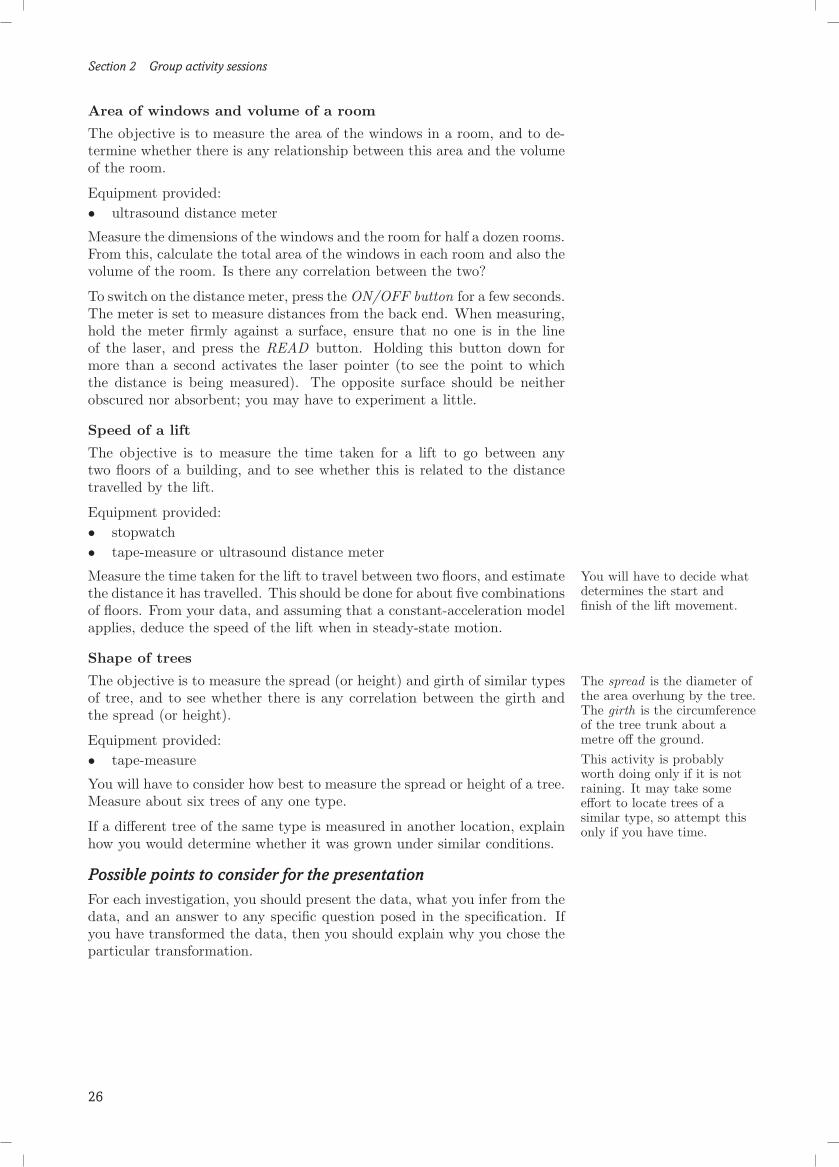
Area of windows and volume of a room
The objective is to measure the area of the windows in a room, and to de-termine whether there is any relationship between this area and the volumeof the room.
Equipment provided:• ultrasound distance meter
Measure the dimensions of the windows and the room for half a dozen rooms.From this, calculate the total area of the windows in each room and also thevolume of the room. Is there any correlation between the two?
To switch on the distance meter, press the ON/OFF button for a few seconds.The meter is set to measure distances from the back end. When measuring,hold the meter firmly against a surface, ensure that no one is in the lineof the laser, and press the READ button. Holding this button down formore than a second activates the laser pointer (to see the point to whichthe distance is being measured). The opposite surface should be neitherobscured nor absorbent; you may have to experiment a little.
Speed of a lift
The objective is to measure the time taken for a lift to go between anytwo floors of a building, and to see whether this is related to the distancetravelled by the lift.
Equipment provided:• stopwatch• tape-measure or ultrasound distance meter
Measure the time taken for the lift to travel between two floors, and estimate You will have to decide whatdetermines the start andfinish of the lift movement.
the distance it has travelled. This should be done for about five combinationsof floors. From your data, and assuming that a constant-acceleration modelapplies, deduce the speed of the lift when in steady-state motion.
Shape of trees
The objective is to measure the spread (or height) and girth of similar types The spread is the diameter ofthe area overhung by the tree.The girth is the circumferenceof the tree trunk about ametre off the ground.This activity is probablyworth doing only if it is notraining. It may take someeffort to locate trees of asimilar type, so attempt thisonly if you have time.
of tree, and to see whether there is any correlation between the girth andthe spread (or height).
Equipment provided:• tape-measure
You will have to consider how best to measure the spread or height of a tree.Measure about six trees of any one type.
If a different tree of the same type is measured in another location, explainhow you would determine whether it was grown under similar conditions.
Possible points to consider for the presentationFor each investigation, you should present the data, what you infer from thedata, and an answer to any specific question posed in the specification. Ifyou have transformed the data, then you should explain why you chose theparticular transformation.
26

Section 2 Group activity sessions
2.4 Sensitivity analysis session
Safety informationAll the work for this session will be based on results from two of the othergroup activities, and there should be no need for further data collection. Itis important that, for this session, you bring the data that you measured inthe other group activities.
AimsThe aims of this session are:• to determine the sensitivity of the final value obtained in a calculation
to changes in the values of input quantities used in the calculation;• to improve your Mathcad skills by using Mathcad to explore sensitivity.
Prerequisite knowledgeFor this session you will need an understanding of partial derivatives, for Partial derivatives are covered
in MST209 Unit 12 .which there are some exercises in Subsection 3.8. You will also need to beable to use Mathcad to plot graphs, to differentiate symbolically and to solvenon-linear algebraic equations.
IntroductionA modelling process usually results in equations that specify the values ofoutput variables or parameters in terms of input variables or parameters. Foran output quantity y, and input quantities x1, x2, x3, this can be representedas shown in Figure 2.16.
Model
✏✏✏✶✲
,,,#Inputs
x3
x2
x1
✲ y
Output
Figure 2.16 Inputs and output for a model
In most situations, the values of the input quantities are not known exactly,and they have some errors associated with them, which lead to a correspond-ing error in the output quantity. This is indicated in Figure 2.17, where δx1,δx2, δx3 are errors in the input quantities x1, x2, x3, respectively, and δy isthe resulting error in the output quantity y.
Model
✏✏✏✶✲
,,,#Inputs
x3 + δx3
x2 + δx2
x1 + δx1
✲ y + δy
Output
Figure 2.17 Inputs and output for a model, with errors
Sensitivity analysis is used to find which input values have most effect onthe final solution of a model. Errors in some of the inputs may have moreeffect on the output value than errors in other inputs.
27

Section 2 Group activity sessions
Definitions of sensitivity
The absolute sensitivity of an output value, y, with respect to changes in aninput value, x, is defined as δy/δx, where δy is the change in y caused by asmall change, δx, in the value of x.
The relative sensitivity of an output value, y, with respect to changes in aninput value, x, is defined as
δy/y
δx/x, that is,
x
y
δy
δx.
If the dimensions, or units, of x and y are different, then it is best to considerthe relative sensitivity, since a change in the unit of measurement will affectthe value of the absolute sensitivity but not that of the relative sensitivity.
There are two ways of determining the sensitivity of the output value tochanges in the input values. The first is an empirical approach, achieved by In the empirical approach,
only one input value at a timeis changed; if more than oneinput value were changed,then the effects of one changemight be masked by those ofanother.
changing the values of each input by a small amount, and then observing theeffect on the solution. The second approach is analytical, based on findingthe rate of change of the output with respect to each of the input quantities.
For the analytical approach, where y = f(x1, x2, . . . , xn):
• the absolute sensitivity of y with respect to xi is∂y
∂xi;
• the relative sensitivity of y with respect to xi isxi
y
∂y
∂xi.
Numerical values for (absolute or relative) sensitivity can be used to com-pare the effects on an output of changes in different inputs, and hence todetermine what changes of input most affect the output.
In the context of mathematical modelling, if the output is unduly sensi-tive to small changes in the value of a parameter, then it may be worthinvestigating the value of this parameter before considering a revision to themodel. Sensitivity analysis may also indicate which modelling assumptions(the ones that introduce this parameter) have most effect on the output andshould be considered for revision. On the other hand, if the output is notsensitive to a parameter value, then this may indicate that the modellingassumptions introducing this parameter are fairly robust and perhaps notcandidates for revision.
Independently of any modelling context, each individual sensitivity valuemeasures the extent to which the output is sensitive to changes in the se-lected input. This raises the question of how large the magnitude of thesensitivity has to be before one can say that ‘the output is sensitive tochanges in the input’. There is no simple answer to this question. In prac-tice, the interpretation of ‘sensitive’ is dependent on the context. However,where the context provides no guidance the following convention may beadopted. An output is regarded as (absolutely or relatively):
• insensitive to changes in an input if the magnitude of the corresponding These criteria are in line withthose adopted for absoluteill-conditioning inMST209 Unit 9 .
sensitivity is less than 5;
• neither sensitive nor insensitive to changes in an input if the magnitudeof the corresponding sensitivity is greater than 5 but less than 10;
• sensitive to changes in an input if the magnitude of the correspondingsensitivity is greater than 10.
28

Section 2 Group activity sessions
The investigationsThis session, on sensitivity, should come after you have completed the ac-tivities on data analysis (Subsection 2.3 on page 16) and at least one of themechanical modelling sessions on the air track (Subsection 2.1 on page 8)or the V-scope (Subsection 2.2 on page 12).
For the presentation, you should include the results of your sensitivity anal-ysis for at least three of the following investigations.
Dissolving a Vitamin C tablet
In this activity, you collected data on the time taken to dissolve a Vita-min C tablet in water whose temperature was measured. From these data,you determined a functional form for the relationship between time takenand water temperature, which involved two parameters whose values wereestimated from the data.
Investigate whether the time taken for a tablet to dissolve, as predicted byyour empirical function, is sensitive to changes in the parameter values.
A damped pendulum
In this activity, you collected data on the angle of swing of a pendulum asa function of the number of oscillations. Over each cycle of oscillation, theamplitude is multiplied by the factor λ (< 1). For small amplitudes, a lineardamping model applies, and for this λ is a constant. In fact, from MST209Unit 17 , the factor is given by
λ = exp(− 2πα√
1− α2
),
where α is the damping ratio.
In the data-analysis session, you should have found that θ = cemN providesthe best fit for the data values, from among the choices on offer. Here θ isthe angle of swing and N is the number of oscillations, while c and m areconstants whose values depend upon your data. Over one oscillation thisgives λ = em, so that
m = − 2πα√1− α2
.
Rearrange this equation to make α the subject, and from this deduce howsensitive the value of α is to changes in the value of m. Determine theconfidence interval for α.
Air track If you have done only one ofthe group activity sessions onthe air track and V-scope,then refer to that particularsection here. If you have doneboth, then you can choosewhichever you prefer.
In this session, you found a value for the period of the motion for a singleglider, and for the periods of the normal mode motion for two gliders. Thenormal mode behaviour was exhibited by releasing the gliders from rest withdisplacements from their equilibrium positions that were in proportion tothe eigenvector element values.
Investigate the sensitivity of each of the following to changes in the measuredvalues of the parameters (masses, stiffnesses):• the periods of motion;• the eigenvector element values.
29

Section 3 Exercises on mathematical methods
V-scope
In the first part of the V-scope session, you obtained a value for the coeffi-cient of sliding friction.
Investigate the sensitivity of this coefficient to changes in the measured slopeof the board.
In the second part of the V-scope session, you investigated the modellingassumption for a pulley. It was suggested that you compare the tensionseither side of the pulley instead of comparing the predicted accelerationwith that found by experiment.
Investigate the sensitivity of each of the predicted acceleration and the dif-ference in tensions to changes in the measured position values.
Possible points to consider for the presentationIn each investigation, you should indicate which of the input values has mosteffect on the output value. You should make use of both the empirical andanalytical approaches, but not necessarily for the same investigation. Yourpresentation should include a discussion of the advantages and disadvantagesof the empirical and analytical approaches.
3 Exercises on mathematical methodsThese exercises have been included to help you revise some of the mathemat- This section covers material
relevant to MST209 Units 2,3 and 9–12 . If you arecurrently studying MST209,then what you do not tacklenow can be used later forrevision purposes.
ical methods that you may need for your mathematical modelling or in thegroup activity sessions. It will be useful to have a good working knowledgeof these topics when you come to the group activity sessions.
The appropriate mathematical methods for each activity are as follows.
Activity Topic Subsection in MST209this booklet unit
Air track Second-order differential equations 3.3 3Systems of linear differential equations 3.7 11
Sensitivity Partial derivatives 3.8 12
The exercises are grouped by topic, and for each chosen topic you shouldtry at least the starred exercises. Do enough on each chosen topic to feelthat you have a good understanding before moving to the next topic.
3.1 Classification of differential equations
Before solving differential equations, it is important to classify them. Clas-sification involves identifying:• the independent variable;• the dependent variable;• the order of the differential equation;• whether it is linear, and if so whether it is constant-coefficient and/or
homogeneous;• any other striking characteristics.
30

Section 3 Exercises on mathematical methods
Exercise 3.1
Classify each of the following differential equations as much as you can.
*(a) xdy
dx+ y3 sin y = 4
*(b)d2x
ds2− 2s + esx = 3
*(c) xdp
dx= 4p− 8
(d)d3p
dy3− 3
d2p
dy2+ 2
dp
dy− 4y = 0
(e) sin(r + 1)dp
dr= 8p− 5r
*(f)d2q
ds2− 2
dq
ds+ 5q = 0
3.2 First-order differential equations
Consider first-order differential equations, i.e. those that can be written in This subsection coversmaterial in MST209 Unit 2 .the form
dy
dx= f(x, y).
There are two main methods of solution for such equations: separation ofvariables and the integrating factor method.
Separation of variablesThis method is applicable to differential equations that can be written inthe form
dy
dx= g(x)h(y). The cases dy/dx = g(x) and
dy/dx = h(y) can be seen asspecial cases of this method.
(3.1)
The technique proceeds as follows. ‘Separate’ dy/dx and the expressionsinvolving y to one side of the equation, and the expressions involving x tothe other side:
1h(y)
dy
dx= g(x) (leaving aside the case h(y) = 0).
Now integrate both sides with respect to x:∫1
h(y)dy
dxdx =
∫g(x) dx.
The left-hand side simplifies by using the rule for integration by substitution,to obtain∫
1h(y)
dy =∫
g(x) dx. (3.2)
The solution of the differential equation is now obtained by performing theintegrations. In practice, it is normal to proceed directly from (3.1) to (3.2).
In general, the solution of a first-order differential equation involves onearbitrary constant of integration and is called the general solution of thedifferential equation. The value of this constant can be found if an initialcondition is provided. This gives a particular solution.
31
Section 3 Exercises on mathematical methods
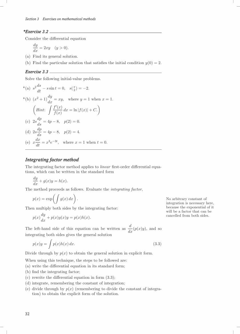
*Exercise 3.2
Consider the differential equation
dy
dx= 2xy (y > 0).
(a) Find its general solution.
(b) Find the particular solution that satisfies the initial condition y(0) = 2.
Exercise 3.3
Solve the following initial-value problems.
*(a) s2 ds
dt− s sin t = 0, s(π
2 ) = −2.
*(b) (x2 + 1)dy
dx= xy, where y = 1 when x = 1.(
Hint :∫
f ′(x)f(x)
dx = ln |f(x)|+ C.
)(c) 2s
dp
ds= 4p− 8, p(2) = 0.
(d) 2sdp
ds= 4p− 8, p(2) = 4.
(e) xdx
dt= x3e−3t, where x = 1 when t = 0.
Integrating factor methodThe integrating factor method applies to linear first-order differential equa-tions, which can be written in the standard form
dy
dx+ g(x)y = h(x).
The method proceeds as follows. Evaluate the integrating factor,
p(x) = exp(∫
g(x) dx
). No arbitrary constant of
integration is necessary here,because the exponential of itwill be a factor that can becancelled from both sides.
Then multiply both sides by the integrating factor:
p(x)dy
dx+ p(x)g(x)y = p(x)h(x).
The left-hand side of this equation can be written asd
dx(p(x)y), and so
integrating both sides gives the general solution
p(x)y =∫
p(x)h(x) dx. (3.3)
Divide through by p(x) to obtain the general solution in explicit form.
When using this technique, the steps to be followed are:(a) write the differential equation in its standard form;(b) find the integrating factor;(c) rewrite the differential equation in form (3.3);(d) integrate, remembering the constant of integration;(e) divide through by p(x) (remembering to divide the constant of integra-
tion) to obtain the explicit form of the solution.
32

Section 3 Exercises on mathematical methods
*Exercise 3.4
Find the general solution of the differential equation
dy
dx= 4− 2y.
Exercise 3.5
Solve the following initial-value problems.
*(a) xdy
dx+ 2y = 4x2 (x ≥ 1), y(1) = 2.
*(b) (x2 + 1)dy
dx= xy, where y = 1 when x = 1.
(c) t2dx
dt+ 5tx = 7t3 + 4 (t ≥ 1), x(1) = 4.
3.3 Linear constant-coefficient differential equations
Try this exercise first to judge whether you need to revise this topic. This subsection coversmaterial in MST209 Unit 3 .
*Exercise 3.6
Find the general solution of the differential equation
3x + 12x = 6.
Linear differential equations of any order which have constant coefficientsmultiplying the unknown function and its derivatives can be solved in a spe-cial way. The first-order case for such differential equations can be writtenin the form
ady
dx+ by = f(x).
The second-order case for such differential equations can be written in theform
ad2y
dx2+ b
dy
dx+ cy = f(x).
Consider first the homogeneous case, where f(x) is the zero function, andthen turn to the inhomogeneous case, where f(x) is a non-zero function of x.
Homogeneous equationsThe form of general solution of the homogeneous differential equation
ad2y
dx2+ b
dy
dx+ cy = 0
depends on the roots of the auxiliary equation, The first-order differentialequation can be considered asa simple version of thesecond-order differentialequation, with a = 0, so thatthe auxiliary equation islinear with only one real root.
aλ2 + bλ + c = 0.
There are three cases, depending on whether this equation has two distinctreal roots, equal roots or complex roots. The corresponding solutions of thedifferential equation are summarized in Table 3.1.
33

Section 3 Exercises on mathematical methods
Table 3.1
Roots of auxiliary equation General solution of differential equation
distinct real roots λ1, λ2 y = Ceλ1x + Deλ2x
equal real roots λ1 = λ2 y = (C + Dx)eλ1x
complex conjugate roots y = eαx(C cos(βx) + D sin(βx))λ1 = α + iβ, λ2 = α− iβ
Exercise 3.7
Find the roots of the auxiliary equations of the following differential equa-tions, and hence find the general solutions of the differential equations.
(a) 3dy
dx− 4y = 0 *(b) 2
dy
dt+ 5y = 0
*(c)d2y
dx2+ 3
dy
dx− 4y = 0 *(d)
d2x
dt2− 4
dx
dt+ 4x = 0
*(e)d2y
dx2+ 2
dy
dx+ 5y = 0 (f)
d2y
dt2− 4
dy
dt= 0
(g)d2y
dx2− 4y = 0 (h)
d2x
dt2+ 4x = 0
Inhomogeneous equationsNow consider inhomogeneous differential equations, of the form
ad2y
dx2+ b
dy
dx+ cy = f(x).
The general solution of this differential equation can be split into two parts:
general solution = complementary function + particular integral.
The complementary function is the general solution of the associated homo-geneous equation,
ad2y
dx2+ b
dy
dx+ cy = 0.
This part contains two arbitrary constants.
A particular integral is any particular solution of the inhomogeneous equa-tion. For common forms of the function f(x), it is possible to find a par-ticular solution by the method of undetermined coefficients . Suitable trialsolutions are given in Table 3.2.
Table 3.2
Right-hand side f(x) Trial solution y(x)
mnxn + mn−1xn−1 + · · ·+ m1x + m0 pnxn + pn−1x
n−1 + · · ·+ p1x + p0
mekx pekx
m cos(Ωx) + n sin(Ωx) p cos(Ωx) + q sin(Ωx)
34

Section 3 Exercises on mathematical methods
The technique for solving inhomogeneous linear constant-coefficient differ-ential equations can be summarized as follows:(a) find the roots of the auxiliary equation, and hence write down the com-
plementary function;(b) find a particular integral by substituting the trial solution (obtained from
Table 3.2) into the inhomogeneous differential equation and equatingcoefficients of corresponding terms;
(c) general solution = complementary function + particular integral.
Exercise 3.8
Find the general solution of the following differential equations. You will find the solutions toExercise 3.7 useful.
*(a) 2dy
dt+ 5y = 10t *(b) 2
dy
dt+ 5y = 3e−2t
(c) 2dy
dt+ 5y = sin(2t) *(d)
d2y
dx2+ 3
dy
dx− 4y = 2e2x
(e)d2x
dt2− 4
dx
dt+ 4x = 4t (f)
d2y
dx2+ 2
dy
dx+ 5y = 2 cos(2x)
Exercise 3.9
Find the solution of the differential equation You will find the solution toExercise 3.8(e) useful.
d2x
dt2− 4
dx
dt+ 4x = 4t
which satisfies the initial conditions
x = 0 anddx
dt= 0 when t = 0.
There is one case where the above procedure for finding a particular solutionfails. This is when the suggested trial solution contains a term that is alsoa solution to the associated homogeneous equation. For example, considerthe differential equation
d2x
dt2− 4
dx
dt+ 4x = e2t.
The complementary function is xc = (C + Dt)e2t = Ce2t + Dte2t (see Exer-cise 3.7(d)). The table suggests the trial solution pe2t, which is a solutionto the associated homogeneous equation, obtained by putting C = p andD = 0 in the complementary function. If this occurs, you should multiplythe suggested trial solution by the independent variable (t in this example)to obtain a new suggested trial solution; if necessary, repeat this procedureuntil the suggested trial solution contains no terms that are solutions to theassociated homogeneous equation.
Exercise 3.10
Find the general solution of the following differential equations. You will find the solutions toExercise 3.7 helpful.
(a) 3dy
dx− 4y = e4x/3
(b)d2y
dx2+ 3
dy
dx− 4y = e−4x
(c)d2x
dt2− 4
dx
dt+ 4x = e2t
35

Section 3 Exercises on mathematical methods
3.4 Gaussian elimination
A system of linear equations can be expressed in matrix form as Ax = b, This subsection coversmaterial in MST209 Unit 9 .where x and b are vectors and A is a square matrix. The problem, in terms
of matrices, is to determine the vector x that satisfies the equation Ax = b.
Example 3.1
Use matrices and the Gaussian elimination method to solve the followingsystem of linear equations. 2x1 + 3x2 − 2x3 = 1
4x1 + 7x2 + 3x3 = 36x1 + 3x2 − 2x3 = −3
Solution
Expressed in terms of matrices and vectors, this becomes
Ax = b,
where
A =
2 3 −24 7 36 3 −2
, x =
x1
x2
x3
, b =
13
−3
.
For computing purposes it is sufficient to record the information in theaugmented matrix:
A|b =
2 3 −2 14 7 3 36 3 −2 −3
R1
R2
R3
Stage 1 : eliminationThe aim here is to reduce the matrix to upper triangular form by subtractingmultiples of one row from others in an orderly fashion. Use the row labelsR1, R2 and R3 to record these row operations.
Stage 1(a): first column
R2 − 2R1
R3 − 3R1
2 3 −2 10 1 7 10 −6 4 −6
R1
R2a
R3a
Stage 1(b): second column
R3a + 6R2a
2 3 −2 10 1 7 10 0 46 0
R1
R2a
R3b
The matrix A is now in upper triangular form.
Stage 2 : back substitutionThe third row gives 46x3 = 0, so x3 = 0. The second row gives x2 + 7x3 = 1,so x2 = 1. The first row gives 2x1 + 3x2 − 2x3 = 1, so x1 = −1. In matrixterms, the solution is x = [−1 1 0]T .
The diagonal elements of the upper triangular matrix (2, 1 and 46 in theabove example) are called pivots. The steps in the Gaussian eliminationmethod (which fails if any of the pivots is zero) are contained in the followingprocedure.
36

Section 3 Exercises on mathematical methods
Gaussian elimination method
To solve a system of n linear equations in n unknowns, with coefficientmatrix A and right-hand-side vector b, carry out the following steps.
(a) Write down the augmented matrix A|b with rows R1, . . . ,Rn.
(b) Subtract multiples of R1 from R2,R3, . . . ,Rn to reduce the ele- Stage 1 : eliminationments below the leading diagonal in the first column to zero. Stage 1(a): first column
In the matrix obtained, subtract multiples of R2 from R3,R4, . . . ,Rn Stage 1(b): second columnto reduce the elements below the leading diagonal in the second col-umn to zero.
Continue this process until A|b is reduced to U|c, where U is an Stage 1(c): . . .upper triangular matrix.
(c) Solve the system of equations with coefficient matrix U and right- Stage 2 : back substitutionhand-side vector c by back substitution to determine the solution.
*Exercise 3.11
Use matrices and the Gaussian elimination method to solve the followingsystem of linear equations. x1 + 3x2 − 2x3 = 3
3x1 + 7x2 + 3x3 = 165x1 + 3x2 − 2x3 = 11
The Gaussian elimination method breaks down if one of the pivots is zero.This can often be rescued by performing an essential row interchange —interchanging the row containing the zero pivot with one of the rows beneathit. However, if the matrix A is singular, the Gaussian elimination methodwill always end up with a zero pivot that cannot be interchanged. In suchcases there will be either no solutions to the system of equations or an infinitenumber of solutions.
Exercise 3.12
Use matrices and the Gaussian elimination method with essential row inter-changes to solve each of the following systems of linear equations.
(a)
2x1 + 3x2 − 2x3 = 14x1 + 6x2 + 3x3 = 26x1 + 3x2 − 2x3 = 9
*(b)
2x1 + 3x2 − 2x3 = 14x1 + 6x2 + 3x3 = 26x1 + 9x2 − 2x3 = 3
(c)
2x1 + 3x2 − 2x3 = 14x1 + 6x2 + 3x3 = 26x1 + 9x2 − 2x3 = 7
37

Section 3 Exercises on mathematical methods
3.5 Determinants
The determinant detA of a square matrix A can be used to determine This subsection coversmaterial in MST209 Unit 9 .whether A is singular. The matrix A is singular if and only if detA = 0.
For the 2× 2 matrix
A =[
a bc d
],
the determinant is defined as
detA =∣∣∣∣ a bc d
∣∣∣∣ = ad− bc.
The determinant of the 3× 3 matrix
A =
a1 a2 a3
b1 b2 b3
c1 c2 c3
is given by
detA = a1
∣∣∣∣ b2 b3
c2 c3
∣∣∣∣− a2
∣∣∣∣ b1 b3
c1 c3
∣∣∣∣ + a3
∣∣∣∣ b1 b2
c1 c2
∣∣∣∣ . Note the minus sign for thesecond term.
Exercise 3.13
Evaluate the determinants of the following matrices.
*(a)[
4 11 2
](b)
[1 24 1
]
(c)
2 3 −24 6 36 3 −2
*(d)
2 3 −20 6 30 0 −2
*(e)
2 3 −24 6 36 9 −2
Which, if any, of these matrices is singular?
3.6 Eigenvalues and eigenvectors
Try this exercise first to judge whether you need to revise this topic. This subsection coversmaterial in MST209 Unit 10 .
*Exercise 3.14
Find the eigenvalues and eigenvectors of the matrix[−7 5
3 −5
].
Suppose that A is a square matrix. Then an eigenvalue λ of A is a numberfor which the equation
(A− λI)v = 0
has a solution other than v = 0. A vector v += 0 satisfying this equation isan eigenvector corresponding to the eigenvalue λ.
If the equation (A − λI)v = 0 has a solution other than v = 0, then thematrix A− λI must be singular. Hence, to find the eigenvalues of A, formthe characteristic equation of A,
det(A− λI) = 0,
and solve this for λ.
38
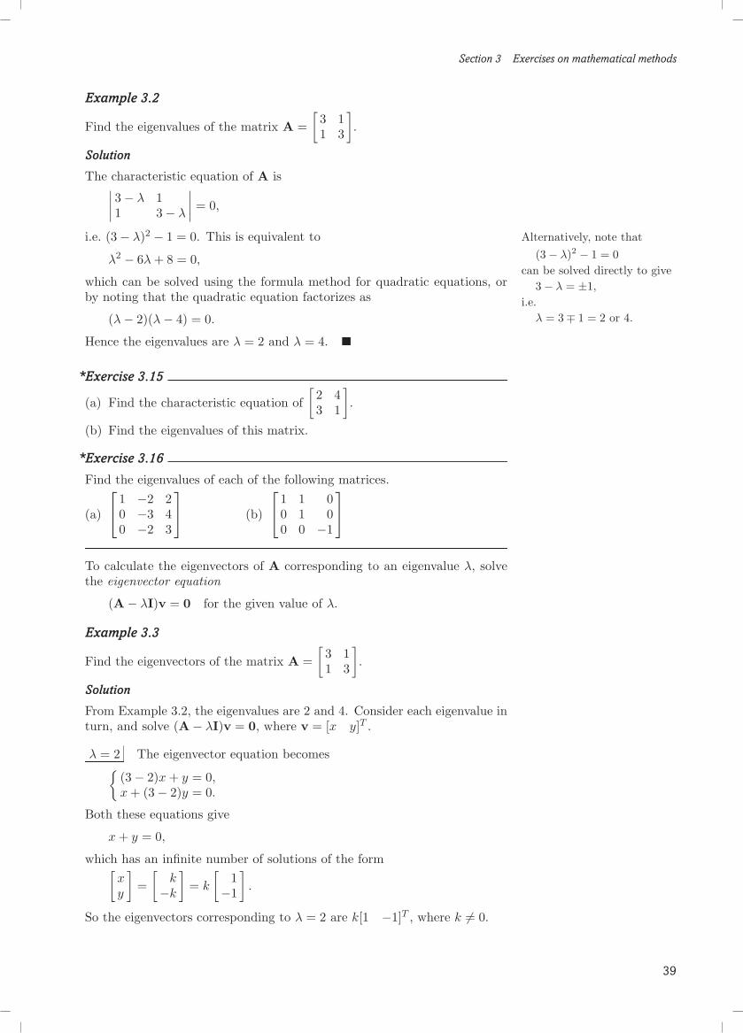
Section 3 Exercises on mathematical methods
Example 3.2
Find the eigenvalues of the matrix A =[
3 11 3
].
Solution
The characteristic equation of A is∣∣∣∣ 3− λ 11 3− λ
∣∣∣∣ = 0,
i.e. (3− λ)2 − 1 = 0. This is equivalent to Alternatively, note that(3− λ)2 − 1 = 0
can be solved directly to give3− λ = ±1,
i.e.λ = 3∓ 1 = 2 or 4.
λ2 − 6λ + 8 = 0,
which can be solved using the formula method for quadratic equations, orby noting that the quadratic equation factorizes as
(λ− 2)(λ− 4) = 0.
Hence the eigenvalues are λ = 2 and λ = 4.
*Exercise 3.15
(a) Find the characteristic equation of[
2 43 1
].
(b) Find the eigenvalues of this matrix.
*Exercise 3.16
Find the eigenvalues of each of the following matrices.
(a)
1 −2 20 −3 40 −2 3
(b)
1 1 00 1 00 0 −1
To calculate the eigenvectors of A corresponding to an eigenvalue λ, solvethe eigenvector equation
(A− λI)v = 0 for the given value of λ.
Example 3.3
Find the eigenvectors of the matrix A =[
3 11 3
].
Solution
From Example 3.2, the eigenvalues are 2 and 4. Consider each eigenvalue inturn, and solve (A− λI)v = 0, where v = [x y]T .
λ = 2 The eigenvector equation becomes{(3− 2)x + y = 0,x + (3− 2)y = 0.
Both these equations give
x + y = 0,
which has an infinite number of solutions of the form[xy
]=
[k
−k
]= k
[1
−1
].
So the eigenvectors corresponding to λ = 2 are k[1 −1]T , where k += 0.
39
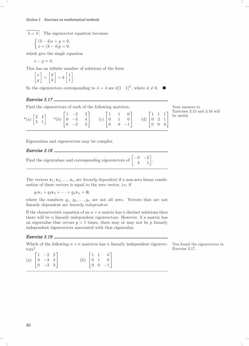
Section 3 Exercises on mathematical methods
λ = 4 The eigenvector equation becomes{(3− 4)x + y = 0,x + (3− 4)y = 0,
which give the single equation
x− y = 0.
This has an infinite number of solutions of the form[xy
]=
[kk
]= k
[11
].
So the eigenvectors corresponding to λ = 4 are k[1 1]T , where k += 0.
Exercise 3.17
Find the eigenvectors of each of the following matrices. Your answers toExercises 3.15 and 3.16 willbe useful.
*(a)[
2 43 1
]*(b)
1 −2 20 −3 40 −2 3
(c)
1 1 00 1 00 0 −1
(d)
1 1 10 2 10 0 3
Eigenvalues and eigenvectors may be complex.
Exercise 3.18
Find the eigenvalues and corresponding eigenvectors of[−3 −2
4 1
].
The vectors v1,v2, . . . ,vn are linearly dependent if a non-zero linear combi-nation of these vectors is equal to the zero vector, i.e. if
q1v1 + q2v2 + · · · + qnvn = 0,
where the numbers q1, q2, . . . , qn are not all zero. Vectors that are notlinearly dependent are linearly independent.
If the characteristic equation of an n×n matrix has n distinct solutions thenthere will be n linearly independent eigenvectors. However, if a matrix hasan eigenvalue that occurs p > 1 times, there may or may not be p linearlyindependent eigenvectors associated with that eigenvalue.
Exercise 3.19
Which of the following n× n matrices has n linearly independent eigenvec- You found the eigenvectors inExercise 3.17.tors?
(a)
1 −2 20 −3 40 −2 3
(b)
1 1 00 1 00 0 −1
40

Section 3 Exercises on mathematical methods
3.7 Systems of linear differential equations
Try this exercise first to judge whether you need to revise this topic. This subsection coversmaterial in MST209 Unit 11 .
*Exercise 3.20
Find the general solution of the pair of simultaneous second-order differentialequations You will find the solution to
Exercise 3.14 helpful.[x1
x2
]=
[−7 53 −5
] [x1
x2
]+
[−37
].
A system of differential equations, such as{x = 2x + 4y + sin ty = 3x + y + cos t,
can be written in matrix form as
x = Ax + h(t),
where
A =[
2 43 1
], x =
[xy
], x =
[xy
]and h(t) =
[sin tcos t
].
A system of differential equations that can be written in the formx = Ax + h(t) is linear and first-order. A system that can be written in theform x = Ax + h(t) is linear and second-order. If h(t) = 0 in either case,the system is homogeneous.
Exercise 3.21
Show that x = veλt (where v is a non-zero constant vector) is a solution ofx = Ax if λ is an eigenvalue of A and v is a corresponding eigenvector.
The result of Exercise 3.21 leads to a procedure for solving a first-orderhomogeneous system x = Ax, so long as the n× n matrix A has n linearlyindependent eigenvectors.
Theorem Suppose that the n × n matrix A has n linearly independenteigenvectors v1,v2, . . . ,vn, corresponding to eigenvalues λ1, λ2, . . . , λn. Thenthe general solution of the system x = Ax is
x = C1v1eλ1t + C2v2e
λ2t + · · ·+ Cnvneλnt,
where C1, C2, . . . , Cn are arbitrary constants.
Exercise 3.22
Using the results of Exercise 3.17 as appropriate, write down the generalsolutions of the systems below.
*(a){
x = 2x + 4yy = 3x + y
(b)
x = x + y + zy = 2y + zz = 3z
*(c)
x = x− 2y + 2zy = − 3y + 4zz = − 2y + 3z
41
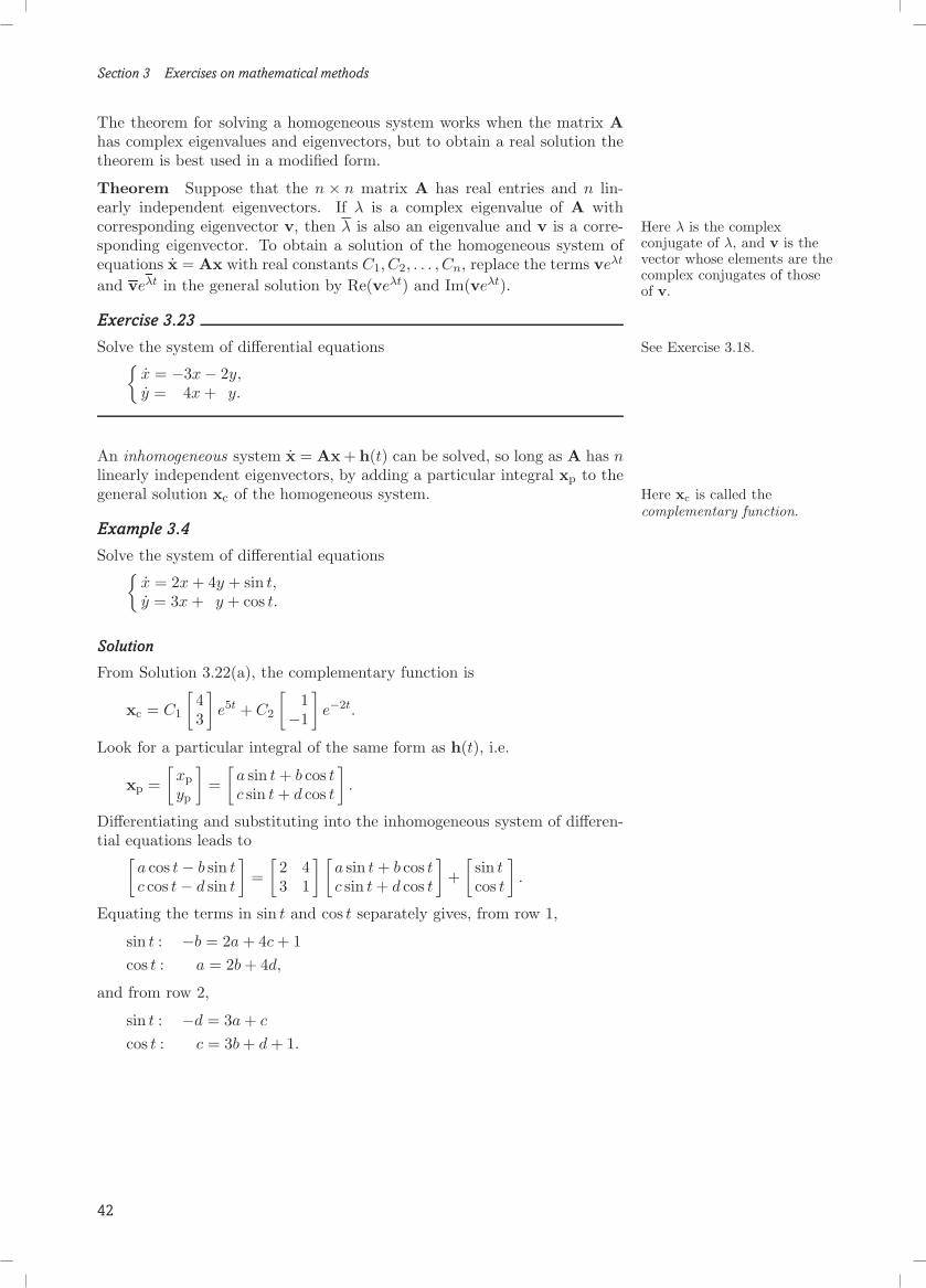
Section 3 Exercises on mathematical methods
The theorem for solving a homogeneous system works when the matrix Ahas complex eigenvalues and eigenvectors, but to obtain a real solution thetheorem is best used in a modified form.
Theorem Suppose that the n × n matrix A has real entries and n lin-early independent eigenvectors. If λ is a complex eigenvalue of A withcorresponding eigenvector v, then λ is also an eigenvalue and v is a corre- Here λ is the complex
conjugate of λ, and v is thevector whose elements are thecomplex conjugates of thoseof v.
sponding eigenvector. To obtain a solution of the homogeneous system ofequations x = Ax with real constants C1, C2, . . . , Cn, replace the terms veλt
and veλt in the general solution by Re(veλt) and Im(veλt).
Exercise 3.23
Solve the system of differential equations See Exercise 3.18.{x = −3x− 2y,y = 4x + y.
An inhomogeneous system x = Ax + h(t) can be solved, so long as A has nlinearly independent eigenvectors, by adding a particular integral xp to thegeneral solution xc of the homogeneous system. Here xc is called the
complementary function.Example 3.4
Solve the system of differential equations{x = 2x + 4y + sin t,y = 3x + y + cos t.
Solution
From Solution 3.22(a), the complementary function is
xc = C1
[43
]e5t + C2
[1
−1
]e−2t.
Look for a particular integral of the same form as h(t), i.e.
xp =[
xp
yp
]=
[a sin t + b cos tc sin t + d cos t
].
Differentiating and substituting into the inhomogeneous system of differen-tial equations leads to[
a cos t− b sin tc cos t− d sin t
]=
[2 43 1
] [a sin t + b cos tc sin t + d cos t
]+
[sin tcos t
].
Equating the terms in sin t and cos t separately gives, from row 1,
sin t : −b = 2a + 4c + 1cos t : a = 2b + 4d,
and from row 2,
sin t : −d = 3a + c
cos t : c = 3b + d + 1.
42

Section 3 Exercises on mathematical methods
These can be written in matrix form as−2 −1 −4 0
1 −2 0 −43 0 1 10 −3 1 −1
abcd
=
1001
.
Using Gaussian elimination, the solution of this system of equations isa = − 2
65 , b = −2965 , c = − 8
65 , d = 1465 , so the particular integral is
xp = 165
[−2 sin t− 29 cos t−8 sin t + 14 cos t
].
The general solution of the inhomogeneous system of differential equationsis
x = xc + xp = C1
[43
]e5t + C2
[1
−1
]e−2t + 1
65
[−2 sin t− 29 cos t−8 sin t + 14 cos t
].
*Exercise 3.24
Solve the following systems of differential equations. You will find the solution toExercise 3.22(c) helpful.
(a)
x = x− 2y + 2z + e2t
y = − 3y + 4z + 4e2t
z = − 2y + 3z + e2t(b)
x = x− 2y + 2z + 2y = − 3y + 4z + 4z = − 2y + 3z + 2
(c)
x = x− 2y + 2z + 2e2t + 2y = − 3y + 4z + 8e2t + 4z = − 2y + 3z + 2e2t + 2
As was noted earlier, a homogeneous second-order system of linear differen-tial equations, such as{
x = 2x + 4y,y = 3x + y,
can be written in the form x = Ax.
Exercise 3.25
(a) What conditions must v ( += 0) and µ satisfy if x = veµt is to be asolution of x = Ax?
(b) What conditions must v ( += 0) and ω satisfy if x = v cos(ωt + φ) andx = v sin(ωt + φ) are to be solutions of x = Ax?
(c) What conditions must v ( += 0) satisfy if x = (C1 + C2t)v is to be asolution of x = Ax?
The results of Exercise 3.25 can be encapsulated into a procedure for solvingcertain linear second-order homogeneous systems.
43

Section 3 Exercises on mathematical methods
Second-order homogeneous linear systemsTo solve a system x = Ax, where A is an n× n matrix with n distinct Complex eigenvalues and
repeated eigenvalues are notdiscussed here, but they canbe dealt with in a fashionsimilar to that of thefirst-order case.
real eigenvalues:(a) find the eigenvalues λ1, λ2, . . . , λn of A and a corresponding set of
eigenvectors v1, v2, . . . ,vn;(b) • each positive eigenvalue, µ2 say, corresponding to an eigenvec-
tor v, gives rise to two linearly independent solutions
veµt and ve−µt;
• each negative eigenvalue, −ω2 say, corresponding to an eigen-vector v, gives rise to two linearly independent solutions
v cos(ωt) and v sin(ωt);
• a zero eigenvalue corresponding to an eigenvector v gives riseto two linearly independent solutions
v and vt;
(c) the general solution is then an arbitrary linear combination of the2n linearly independent solutions found in (b), involving 2n arbi-trary constants.
Exercise 3.26
Using the results of Exercise 3.17 as appropriate, write down the generalsolutions of the following systems.
*(a){
x = 2x + 4yy = 3x + y
(b)
x = x + y + zy = 2y + zz = 3z
*(c)
x = x− 2y + 2zy = − 3y + 4zz = − 2y + 3z
3.8 Partial derivatives
Try this exercise first to judge whether you need to revise this topic. This subsection coversmaterial in MST209 Unit 12 .
*Exercise 3.27
Find the first and second partial derivatives of
f(x, y) = x1/3y − sin(xy2) (x += 0).
If you were unsure of the solution to the above, here are some more examplesfor practice.
Exercise 3.28
Find the first and second partial derivatives of each of the following func-tions.
(a) f(x, y) = πx3y4
(b) f(x, y) = xyex+y
(c) f(x, y) = sin(x/y) (y += 0)
44

Section 4 Exercises on mechanics
4 Exercises on mechanicsThese exercises have been included to help you revise some of the mechanics This section covers material
relevant to MST209Units 5–8, 14 and 16–18 . Ifyou are currently studyingMST209, then what you donot tackle now can be usedlater for revision purposes.
that you may need for your mathematical modelling or in the group activitysessions. It will be useful to have a good working knowledge of these topicswhen you come to the group activity sessions.
The appropriate mechanics topics for each activity are as follows.
Activity Topic Subsection in MST209this booklet unit
Air track Oscillations 4.4 7Normal modes 4.8 18
V-scope Static objects 4.2 5One-dimensional motion 4.3 6
Some of these mechanics topics rely on a working knowledge of the appro-priate mathematical methods, which are covered in Section 3.
The exercises are grouped by topic, and for each chosen topic you shouldtry at least the starred exercises. Do enough on each chosen topic to feelthat you have a good understanding before moving to the next topic.
4.1 Forces
Try the following exercise to judge whether you need to revise the topics inthis and the following subsection. This subsection covers
material in MST209 Unit 5 .*Exercise 4.1
A particle of mass m rests on a rough plane which is inclined at an angle θ
Figure 4.1
to the horizontal. The coefficient of static friction between the particle andthe plane is µ (where µ < tan θ). A force P, directed parallel to the slope,acts on the particle in the vertical plane containing a line of greatest slope,as shown in Figure 4.1. What is the maximum possible magnitude of theforce for which the particle will remain stationary?
Expressing forces (which are vectors) as the sum of projections onto thedirections of Cartesian unit vectors is often a key step in solving mechanicsproblems. The projection of a vector F onto a unit vector e is (|F| cos θ)e,where θ is the angle between F and e.
When calculating projections, it often simplifies matters to use the standardtrigonometric identities for the cosine of a sum or difference of two angles,
cos(A + B) = cos A cos B − sin A sin B,
cos(A−B) = cos A cos B + sin A sin B.
For example, the following results can be applied:
cos(π2 − α) = cos π
2 cos α + sin π2 sin α = sin α;
cos(π2 + α) = cos π
2 cos α− sin π2 sin α = − sin α;
cos(π− α) = cos π cos α + sin π sin α = − cosα;
cos(π + α) = cos π cosα− sin π sin α = − cosα.
Projecting a force onto a base set of vectors is called resolving the force intoits components relative to the set of vectors.
45
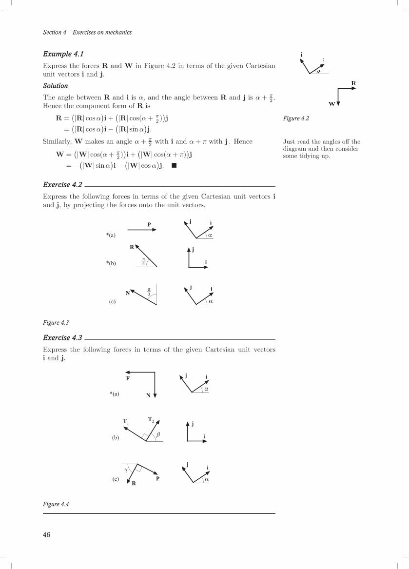
Section 4 Exercises on mechanics
Example 4.1
Express the forces R and W in Figure 4.2 in terms of the given Cartesianunit vectors i and j.
Solution
The angle between R and i is α, and the angle between R and j is α + π2 .
Hence the component form of R is
R =(|R| cos α
)i +
(|R| cos(α + π2 )
)j Figure 4.2
=(|R| cos α
)i− (|R| sin α
)j.
Similarly, W makes an angle α + π2 with i and α + π with j . Hence Just read the angles off the
diagram and then considersome tidying up.W =
(|W| cos(α + π2 )
)i +
(|W| cos(α + π))j
= −(|W| sin α)i− (|W| cos α
)j.
Exercise 4.2
Express the following forces in terms of the given Cartesian unit vectors iand j, by projecting the forces onto the unit vectors.
*
%#a$
%#b$
#c$
+
+
*
+ *
Q
L
O
3π
α
4π
α
Figure 4.3
Exercise 4.3
Express the following forces in terms of the given Cartesian unit vectorsi and j.
%#a$
#b$
#c$
*+
Q
L
D
O
+S,S.
*β
α
*+
γα
Figure 4.4
46

Section 4 Exercises on mechanics
Table 4.1 lists some commonly occurring forces and indicates how they are All of these forces areintroduced in MST209.modelled.
Table 4.1
Force Symbol Magnitude and direction
weight W mg downwards, where m is the mass of the objectnormalreaction
N any magnitude and at right angles to the common tan-gent plane of contact between two surfaces
friction(static)
F |F| ≤ µ|N| (where µ is the coefficient of static friction,assumed constant), opposing any possible motion andperpendicular to the normal reaction
friction(sliding)
F |F| = µ′|N| (where µ′ < µ is the coefficient of slidingfriction, assumed constant), opposing the motion andperpendicular to the normal reaction
string tensionforce
T any magnitude and along the length of the string fromthe point of attachment towards the centre of string
spring force H −k(l − l0)s, where s is a unit vector in the directionfrom the centre of the spring to the point of attachmentof the object, k is the stiffness of the spring, l is itslength and l0 is its natural length
air resistance(linear)
R −c1Dv, where v is the velocity, D is the effective di-ameter of the object, and c1 / 1.7× 10⁻⁴; this modelis valid for D|v| " 10−5
air resistance(quadratic)
R −c2D2|v|v, where v is the velocity, D is the effective
diameter of the object, and c2 / 0.20; this model isvalid for 10−2 " D|v| " 1
Where there is more than one force of the same type, then we commonlyuse subscripts to distinguish between them. Also, F is commonly used fora general force and not just for friction.
4.2 Static objects
The equilibrium condition for static objects is: This subsection coversmaterial in MST209 Unit 5 .(a) the vector sum of the forces acting on the object is zero;
(b) the vector sum of the torques acting on the object is zero.
If the object is a particle, then (b) is always satisfied if (a) is satisfied.
Solving statics problems
Given a statics problem, perform some or all of the following steps.(a) Draw a sketch of the physical situation and annotate it with any
relevant information.(b) Choose coordinate axes, and mark them on your sketch.(c) Draw a force diagram for each object or particle.(d) Use the equilibrium condition and any other appropriate law(s) to
obtain equation(s).(e) Solve the equation(s).(f) Interpret the solution in terms of the original problem.
47

Section 4 Exercises on mechanics
*Exercise 4.4
A particle of mass 5 kg is suspended from the ceiling by a model spring ofstiffness 50Nm−1 and natural length 1m. It is also attached by a modelspring of stiffness 100N m−1 and natural length 0.5 m to the floor at a pointvertically below the point of attachment to the ceiling. The ceiling is 3mabove the floor. How high above the floor is the particle when stationary?What are then the tensions in each of the model springs?
*Exercise 4.5
A jib crane of uniform cross-section, with length 10 m and mass 40 kg, is
3)1 .
.1 ,(
0+h
2+h
Figure 4.5
joined to the side of a ship’s mast by a hinge. The crane is held at an angleof 60◦ to the vertical by a light rope, which is attached to a point 7.5 m alongthe length of the crane from the hinge, as shown in Figure 4.5. The ropemakes an angle of 40◦ to the vertical. A crate of mass 25 kg is suspendedfrom the end of the crane by a light cable. Find the tension in the rope.
Exercise 4.6
A particle of mass m is suspended from the ceiling by a model spring ofstiffness k and natural length l0. It is also attached by a model string oflength 0.5 m to the floor at a point vertically below the point of attachmentto the ceiling. The ceiling is 3 m above the floor. How high above the flooris the particle when stationary? What are then the tensions in the modelspring and in the model string?
(Hint : You will need to consider three cases.)
Exercise 4.7
A particle of mass m rests on a rough plane which is inclined at an angle θO
.
θ
Figure 4.6
to the horizontal. The coefficient of static friction between the particle andthe plane is µ (where µ < tan θ). A horizontal force P acts on the particle inthe vertical plane containing a line of greatest slope, as shown in Figure 4.6.Find the range of magnitudes of the horizontal force for which the particlewill not move up or down the plane.
4.3 One-dimensional motion
Position, velocity and accelerationConsider the motion of a particle. After choosing an origin O and the i-, j-, This subsection covers
material in MST209 Unit 6 .and k-directions, the position vector r(t) specifies the position of the particleat time t. Then the velocity vector v(t) of the particle is
v =drdt
= r
and its acceleration vector a(t) is
a =dvdt
=d2rdt2
= r.
The acceleration in one-dimensional motion in the direction of i can also befound using the formulae
a =dv
dt=
d2x
dt2= v
dv
dx,
where a(t) = a(t)i, v(t) = v(t)i, r(t) = x(t)i.
48
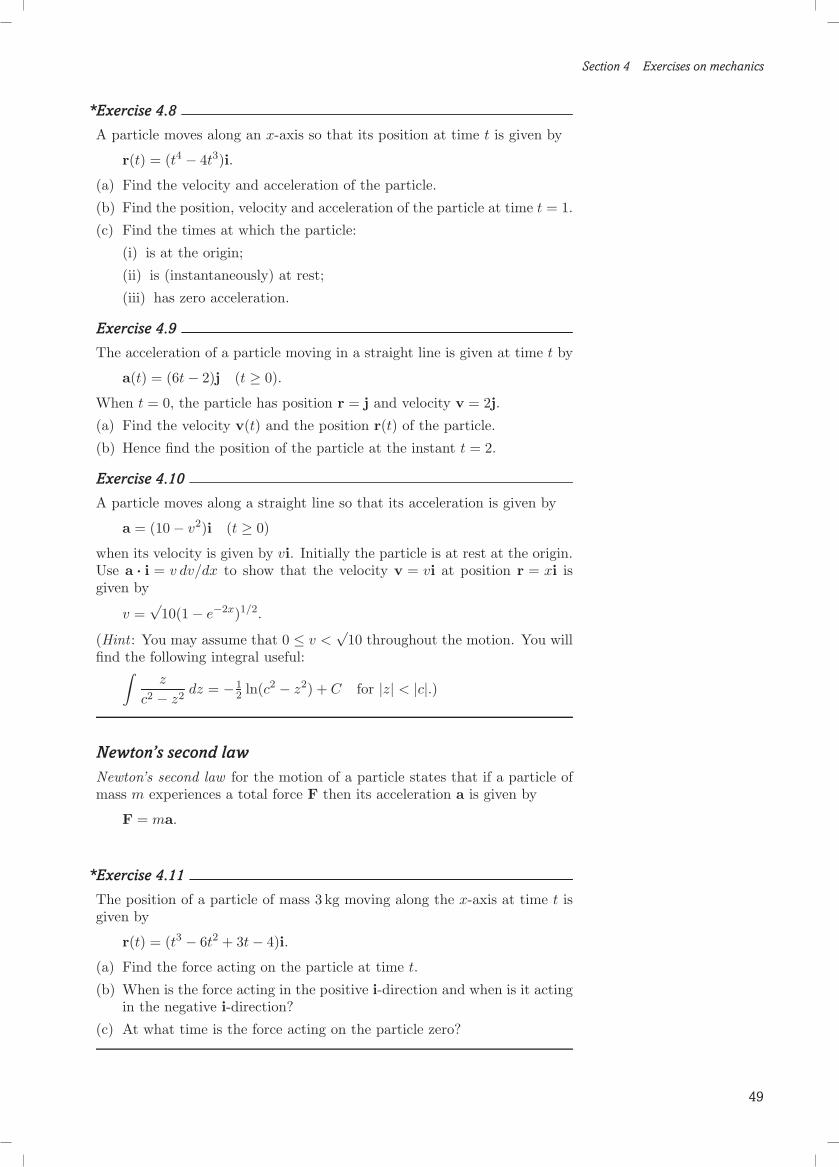
Section 4 Exercises on mechanics
*Exercise 4.8
A particle moves along an x-axis so that its position at time t is given by
r(t) = (t4 − 4t3)i.
(a) Find the velocity and acceleration of the particle.
(b) Find the position, velocity and acceleration of the particle at time t = 1.
(c) Find the times at which the particle:
(i) is at the origin;
(ii) is (instantaneously) at rest;
(iii) has zero acceleration.
Exercise 4.9
The acceleration of a particle moving in a straight line is given at time t by
a(t) = (6t− 2)j (t ≥ 0).
When t = 0, the particle has position r = j and velocity v = 2j.
(a) Find the velocity v(t) and the position r(t) of the particle.
(b) Hence find the position of the particle at the instant t = 2.
Exercise 4.10
A particle moves along a straight line so that its acceleration is given by
a = (10− v2)i (t ≥ 0)
when its velocity is given by vi. Initially the particle is at rest at the origin.Use a . i = v dv/dx to show that the velocity v = vi at position r = xi isgiven by
v =√
10(1− e−2x)1/2.
(Hint : You may assume that 0 ≤ v <√
10 throughout the motion. You willfind the following integral useful:∫
z
c2 − z2dz = −1
2 ln(c2 − z2) + C for |z| < |c|.)
Newton’s second lawNewton’s second law for the motion of a particle states that if a particle ofmass m experiences a total force F then its acceleration a is given by
F = ma.
*Exercise 4.11
The position of a particle of mass 3 kg moving along the x-axis at time t isgiven by
r(t) = (t3 − 6t2 + 3t− 4)i.
(a) Find the force acting on the particle at time t.
(b) When is the force acting in the positive i-direction and when is it actingin the negative i-direction?
(c) At what time is the force acting on the particle zero?
49

Section 4 Exercises on mechanics
When using Newton’s second law to derive the equation of motion, it is oftenconvenient to choose an x-axis for which position and velocity are alwayspositive, if this is possible.
Applying Newton’s second law
Given a mechanics problem involving one-dimensional motion in whicha question regarding the motion is to be answered, proceed as follows.(a) Draw a sketch of the physical situation and annotate it with any
relevant information.(b) Choose the x-axis to lie along the direction of motion and select an
origin. Mark the x-axis, its direction and the origin on your sketch.(c) Draw a force diagram.(d) Apply Newton’s second law to obtain a vector equation. Substitute
the value of each of the forces into the equation and project theequation onto the x-axis to obtain a scalar equation of motion.
(e) Substitute v dv/dx, dv/dt or d2x/dt2 for the acceleration a in thescalar equation of motion and solve the resulting differential equa-tion(s) to obtain the velocity v in terms of the position x or time t,or the position x in terms of the time t, as appropriate.
(f) Interpret the solution in terms of the original problem.
Exercise 4.12
A marble is dropped from rest from the top of a 10m-high tower into a poolof water 1m deep.
(a) Choose a suitable x-axis, and use Newton’s second law to find the equa-tion of motion of the marble before it hits the water, assuming that thenthe only force acting on the marble is the force of gravity.
(b) Hence find the total time of fall and the speed of the marble just beforeit hits the water.
(c) The marble is 1 cm in diameter and has a mass of 25 g. Find the speedwith which it hits the bottom of the pool.
(Hint : When the particle is travelling in water, the drag force on theparticle is given by the linear model R / −0.0094Dv when D|v| " 10−6
and by the quadratic model R / −156D|v|v when 10−3 " D|v| " 10−1.You may also find the following integral useful:∫
z
z2 − c2dz = 1
2 ln(z2 − c2) + C for |z| > |c|.)
*Exercise 4.13
A particle of mass m is thrown vertically upwards with initial speed v0.Assuming that the only forces acting on the particle are gravity and airresistance proportional to the particle’s speed, find how the speed of theparticle varies with time during the particle’s upward motion. Find thetime at which the particle reaches its maximum height.
50

Section 4 Exercises on mechanics
4.4 Oscillations
Try this exercise first to judge whether you need to revise this topic. This subsection coversmaterial in MST209 Unit 7 .
*Exercise 4.14
A particle P of mass 3 kg, attached to two model springs AP and PB,moves along a frictionless horizontal track. The other ends of the springsare fixed to two points A and B a distance 1m apart. Spring AP has stiffness8Nm−1 and natural length 0.5 m, whereas spring PB has stiffness 4 Nm−1
and natural length 0.5 m.
(a) Derive the equation of motion of the particle if the x-axis is chosen withits origin at the fixed point A and direction towards the fixed point B.
(b) Find the particle’s period of oscillations and its equilibrium position. You may find the solution toExercise 3.6 helpful.
Simple harmonic motionThe suggested approach for deriving an equation of motion for a particlesubject to forces due to model springs is as follows.(a) For each spring, find a formula for its length and so for its extension or
compression.(b) For each spring, write down the spring force using Hooke’s law.(c) Apply Newton’s second law to the particle.
If a particle is in one-dimensional motion under the action of model springsand possibly gravity, the equation of motion takes the form
x + ω2x = ω2xeq,
where xeq is the particle’s equilibrium position. The general solution is
x = xeq + B cos(ωt) + C sin(ωt),
or equivalently,
x = xeq + A cos(ωt + φ).
The period of the oscillations is τ = 2π/ω. The amplitude is A =√
B2 + C2
and the phase angle is given by
φ ={
arccos(B/A) for C ≤ 0,− arccos(B/A) for C > 0.
*Exercise 4.15
A particle of mass 4 kg is suspended from the ceiling by a model spring ofstiffness 36N m−1 and natural length 0.2 m. Find the forces acting on theparticle and hence the equation of motion of the particle. What is the periodof oscillation of the particle? If the particle is released from rest 0.5 m belowthe ceiling, what is the lowest that it will go?
*Exercise 4.16
A particle P of mass m, attached to two model springs AP and PB, movesalong a frictionless horizontal track. The other ends of the springs are fixedto two points A and B a distance 3l0 apart. Spring AP has stiffness k andnatural length l0, whereas spring PB has stiffness 2k and natural length l0.
(a) Derive the equation of motion of the particle if the x-axis is chosen withits origin at the fixed point A and direction towards the fixed point B.
(b) Find the particle’s period of oscillations and its equilibrium position.
51

Section 4 Exercises on mechanics
Exercise 4.17
A particle moves along the x-axis so that its position r = xi at time t satisfies
x + 4x = 0.
When t = 0, the position of the particle is given by x = 4 and its velocityby x = 6.
(a) Derive expressions x(t)i for the position of the particle and x(t)i for thevelocity of the particle.
(b) Find the amplitude of the particle’s oscillations.
(c) What are the particle’s position and velocity at time t = 18π?
4.5 Conservation of energy
Suppose that a particle of mass m moves on a straight line (the x-axis), This subsection coversmaterial in MST209 Unit 8 .and at time t has position xi and velocity vi. The law of conservation
of mechanical energy states that, if the total force on the particle has anx-component F (x) that depends only on the particle’s position, then thetotal mechanical energy E = T + U is constant, where T (v) = 1
2mv2 is theparticle’s kinetic energy and U(x) = − ∫
F (x) dx is the particle’s potentialenergy.
The gravitational potential energy is U = mg× height, where the height is The gravitational potentialenergy will be negative if theparticle’s position is belowthe datum.
measured vertically upwards from some chosen datum.
The potential energy for a model spring is U = 12 × stiffness× (deformation)2,
where the datum is chosen at the natural length of the spring.
Applying conservation of energy
A mechanics problem involving the one-dimensional motion of a parti-cle, in which the total force depends only on the position of the particle(or is constant), and where the question to be answered refers to a rela-tionship between the position xi and velocity vi of the particle, can besolved using the law of conservation of mechanical energy by adoptingthe following procedure.(a) Find the potential energy function. This may be done directly
where the form of the potential energy function is already known, aswith gravity or model springs; otherwise one must use the definitionU(x) = − ∫
F (x) dx. If there is more than one force acting on theparticle, then the potential energy function can be found for eachforce in turn, and the results summed to obtain the overall potentialenergy function U(x).
(b) The expression for U(x) will involve an arbitrary constant. Choosethe value for this constant so as to simplify the expression as far aspossible.
(c) Use information provided for the values of x and v at one and thesame time to calculate the (constant) value of the total mechanicalenergy E.
(d) Solve the resulting version of the equation T + U = E, either for x(at a specified value of v) or for v (at a specified value of x).
52

Section 4 Exercises on mechanics
*Exercise 4.18
A ball is thrown vertically upwards with a speed of 20 m s−1. Assuming thatair resistance can be neglected, use the law of conservation of mechanicalenergy to find
(a) the maximum height reached by the ball;
(b) the speed of the ball when its height is 15 m.
Exercise 4.19
A particle of mass 5 kg is hung from a fixed point by a model spring ofnatural length 0.2 m and stiffness 40 Nm−1. The particle is released fromrest when the spring has its natural length. By using the law of conservationof mechanical energy, find the maximum length of the spring during theparticle’s subsequent oscillations.
4.6 Projectiles
A projectile subject to gravity alone moves in a vertical plane. Its equation This subsection coversmaterial in MST209 Unit 14 .of motion is
r = −gj,
where the y-axis is taken vertically upwards and j is a unit vector in thisdirection. Suppose that the projectile is launched from (0,H) at time t = 0with launch speed u at an angle θ to the horizontal. The initial conditionsare r(0) = Hj and r(0) = (u cos θ)i + (u sin θ)j, where i is a unit vector inthe appropriate horizontal direction. The solution of the equation of motionis
r(t) = (ut cos θ)i +(H + ut sin θ− 1
2gt2)j. (4.1)
The projectile’s trajectory is a parabola whose equation (derived from Equa-tion (4.1)) is
y = H + x tan θ− x2 g
2u2
(1 + tan2 θ
). (4.2)
A projectile moving under gravity alone, whose points of launch and impactare in the same horizontal plane (i.e. H = 0), whose initial speed is u andwhose launch angle is θ, has range
R =u2 sin(2θ)
g.
If the point of launch is height H above the horizontal plane on which theprojectile lands, then the maximum range is
Rmax =√
L2 + 2LH, (4.3)
where L = u2/g, and is achieved using the launch angle
θ = arctan(
1√1 + 2H/L
).
To choose a launch angle so that a particular target is hit, first write downthe equation that ensures that the projectile’s trajectory passes through thetarget. This will be a quadratic equation for tan θ; solve it for tan θ. Ifthe quadratic has real roots then the target is achievable. If the quadraticequation does not have real roots then there is no launch angle (given thelaunch speed) that enables the target to be hit.
53

Section 4 Exercises on mechanics
*Exercise 4.20
A stone is thrown from a point O which is at the top of a cliff 10m abovea horizontal beach. The stone is thrown at 20 m s−1 and its launch angle isθ above the horizontal. The stone hits the beach at a horizontal distance of40 m from O. You may neglect any effects due to air resistance. Find thepossible launch angles θ. What is the furthest distance from O to which thestone can be thrown from the top of the cliff, with the same launch speedas before?
*Exercise 4.21
Jane, who works in an office, wishes to throw a box of matches to hit hercolleague on the head. They are separated by a partition that is 2.5 m high.Her colleague sits in such a way that his head is 2m away from the partitionand 1.5 m off the ground. Jane is 2 m away from the partition and shelaunches the box of matches from a height of 1m at a speed of 2
√2g m s−1.
Is it possible for Jane to hit her colleague on his head?
Exercise 4.22
Cinema films often show police chases across the roofs of buildings. Assumethat a policeman can run at 9 m s−1 and can take off at angles up to 1
9πradians (20◦) from the horizontal at this speed. The roof onto which he isjumping is 2m lower than the roof from which he takes off. What is thewidest gap that he can jump?
4.7 Damping, forcing and resonance
Try this exercise first to judge whether you need to revise this topic. This subsection coversmaterial in MST209 Unit 17 .
*Exercise 4.23
The equation of motion of an oscillating system with damping is modelledby the equation of motion
3x + 2x + 12x = 6,
where x (in m) is the displacement of the particle from a fixed point.
(a) Find the damping ratio, natural angular frequency and period of themotion, and the equilibrium position of the particle.
(b) Find the particular solution of the equation of motion for which theparticle is released from rest when x = 1.
(c) What is the time after which the particle remains always within 0.1 mof its equilibrium position?
The simple harmonic oscillator model, with no dissipative elements, can beextended by adding a new element, called a model damper. A schematicdiagram of a particle attached to a model damper is shown in Figure 4.7.
-
4
Figure 4.7
The particle here experiences a force given by
R = −rl s,
where l is the rate of change of length of the model damper, s is a unit vectorin the direction from the centre of the model damper towards the particle,and r is a positive constant called the damping constant.
54
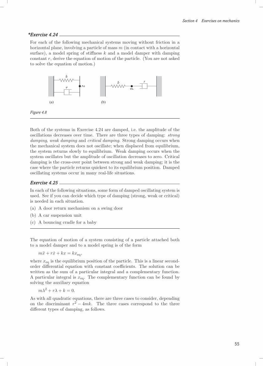
Section 4 Exercises on mechanics
*Exercise 4.24
For each of the following mechanical systems moving without friction in ahorizontal plane, involving a particle of mass m (in contact with a horizontalsurface), a model spring of stiffness k and a model damper with dampingconstant r, derive the equation of motion of the particle. (You are not askedto solve the equation of motion.)
#a$ #b$
Figure 4.8
Both of the systems in Exercise 4.24 are damped, i.e. the amplitude of theoscillations decreases over time. There are three types of damping: strongdamping, weak damping and critical damping. Strong damping occurs whenthe mechanical system does not oscillate; when displaced from equilibrium,the system returns slowly to equilibrium. Weak damping occurs when thesystem oscillates but the amplitude of oscillation decreases to zero. Criticaldamping is the cross-over point between strong and weak damping; it is thecase where the particle returns quickest to its equilibrium position. Dampedoscillating systems occur in many real-life situations.
Exercise 4.25
In each of the following situations, some form of damped oscillating system isused. See if you can decide which type of damping (strong, weak or critical)is needed in each situation.
(a) A door return mechanism on a swing door
(b) A car suspension unit
(c) A bouncing cradle for a baby
The equation of motion of a system consisting of a particle attached bothto a model damper and to a model spring is of the form
mx + rx + kx = kxeq,
where xeq is the equilibrium position of the particle. This is a linear second-order differential equation with constant coefficients. The solution can bewritten as the sum of a particular integral and a complementary function.A particular integral is xeq. The complementary function can be found bysolving the auxiliary equation
mλ2 + rλ + k = 0.
As with all quadratic equations, there are three cases to consider, dependingon the discriminant r2 − 4mk. The three cases correspond to the threedifferent types of damping, as follows.
55
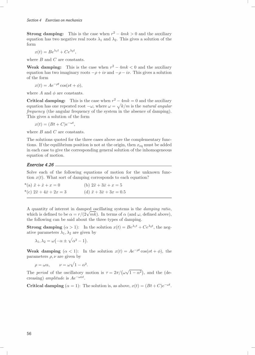
Section 4 Exercises on mechanics
Strong damping: This is the case when r2 − 4mk > 0 and the auxiliaryequation has two negative real roots λ1 and λ2. This gives a solution of theform
x(t) = Beλ1t + Ceλ2t,
where B and C are constants.
Weak damping: This is the case when r2 − 4mk < 0 and the auxiliaryequation has two imaginary roots −ρ + iν and −ρ− iν. This gives a solutionof the form
x(t) = Ae−ρt cos(νt + φ),
where A and φ are constants.
Critical damping: This is the case when r2 − 4mk = 0 and the auxiliaryequation has one repeated root −ω, where ω =
√k/m is the natural angular
frequency (the angular frequency of the system in the absence of damping).This gives a solution of the form
x(t) = (Bt + C)e−ωt,
where B and C are constants.
The solutions quoted for the three cases above are the complementary func-tions. If the equilibrium position is not at the origin, then xeq must be addedin each case to give the corresponding general solution of the inhomogeneousequation of motion.
Exercise 4.26
Solve each of the following equations of motion for the unknown func-tion x(t). What sort of damping corresponds to each equation?
*(a) x + x + x = 0 (b) 2x + 3x + x = 5
*(c) 2x + 4x + 2x = 3 (d) x + 3x + 3x = 0.5
A quantity of interest in damped oscillating systems is the damping ratio,which is defined to be α = r/(2
√mk). In terms of α (and ω, defined above),
the following can be said about the three types of damping.
Strong damping (α > 1): In the solution x(t) = Beλ1t + Ceλ2t, the neg-ative parameters λ1, λ2 are given by
λ1, λ2 = ω(−α±
√α2 − 1
).
Weak damping (α < 1): In the solution x(t) = Ae−ρt cos(νt + φ), theparameters ρ, ν are given by
ρ = ωα, ν = ω√
1− α2.
The period of the oscillatory motion is τ = 2π/(ω√
1− α2), and the (de-
creasing) amplitude is Ae−ωαt.
Critical damping (α = 1): The solution is, as above, x(t) = (Bt + C)e−ωt.
56
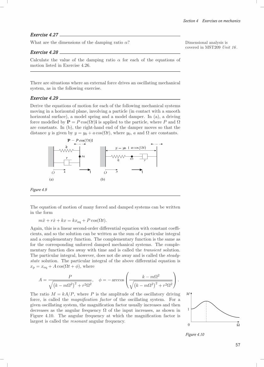
Section 4 Exercises on mechanics
Exercise 4.27
What are the dimensions of the damping ratio α? Dimensional analysis iscovered in MST209 Unit 16 .
Exercise 4.28
Calculate the value of the damping ratio α for each of the equations ofmotion listed in Exercise 4.26.
There are situations where an external force drives an oscillating mechanicalsystem, as in the following exercise.
Exercise 4.29
Derive the equations of motion for each of the following mechanical systemsmoving in a horizontal plane, involving a particle (in contact with a smoothhorizontal surface), a model spring and a model damper. In (a), a drivingforce modelled by P = P cos(Ωt)i is applied to the particle, where P and Ωare constants. In (b), the right-hand end of the damper moves so that thedistance y is given by y = y0 + a cos(Ωt), where y0, a and Ω are constants.
#a$ #b$
Figure 4.9
The equation of motion of many forced and damped systems can be writtenin the form
mx + rx + kx = kxeq + P cos(Ωt).
Again, this is a linear second-order differential equation with constant coeffi-cients, and so the solution can be written as the sum of a particular integraland a complementary function. The complementary function is the same asfor the corresponding unforced damped mechanical systems. The comple-mentary function dies away with time and is called the transient solution.The particular integral, however, does not die away and is called the steady-state solution. The particular integral of the above differential equation isxp = xeq + A cos(Ωt + φ), where
A =P√(
k −mΩ2)2 + r2Ω2
, φ = − arccos
k −mΩ2√(k −mΩ2
)2 + r2Ω2
.
The ratio M = kA/P , where P is the amplitude of the oscillatory driving K
'+
,
Figure 4.10
force, is called the magnification factor of the oscillating system. For agiven oscillating system, the magnification factor usually increases and thendecreases as the angular frequency Ω of the input increases, as shown inFigure 4.10. The angular frequency at which the magnification factor islargest is called the resonant angular frequency.
57

Section 4 Exercises on mechanics
*Exercise 4.30
The equation of motion of an oscillating mechanical system is
x + x + x = 2 cos(Ωt),
where x is the displacement of a particle from equilibrium and Ω is theangular frequency of the forcing input to the system.
(a) Show that the magnification factor for this system can be written as
M =1√
1− Ω2 + Ω4.
(b) Calculate the magnification factor for Ω = 0.1, 0.2, 0.6, 0.7, 0.8, 1.0, 1.5.Give your answers to two decimal places.
(c) Draw a sketch graph of the variation of the magnification factor withthe forcing angular frequency Ω.
(d) From your graph, estimate the resonant angular frequency of the system.
(e) The magnification factor in part (a) has a local maximum when the terminside the square root has a local minimum. The quartic expression1 − Ω2 + Ω4 can be written as a quadratic expression in x = Ω2, asf(x) = 1− x + x2. Show that f(x) has a local minimum when x = 1
2 .
(f) Use your answer to part (e) to calculate the resonant angular frequencyto four decimal places.
4.8 Normal modes
Try this exercise first to judge whether you need to revise this topic. This subsection coversmaterial in MST209 Unit 18 .
*Exercise 4.31
Two particles, P and Q, move along a straight frictionless horizontal track.Particle P , of mass 3 kg, is connected on its left to a fixed point, A, by amodel spring of stiffness 6Nm−1 and natural length 1 m. On its right, P isconnected to a second particle Q, of mass 5 kg, by a model spring of stiffness15 Nm−1 and natural length 1m. Particle Q is connected on its right to afixed point, B, by a model spring of stiffness 10 Nm−1 and natural length2 m. The distance AB is 4m. The distances of the two particles from theleft-hand fixed point are x1 and x2, respectively.
(a) Derive the equations of motion of the two particles, and express themas a single equation in matrix form.
(b) Find the particular motion of the system for which the initial conditions You will find the solution toExercise 3.20 helpful.are [
x1(0)x2(0)
]=
[1.51.7
],
[x1(0)x2(0)
]=
[00
].
The key concept of many-particle systems (and also some one-particle sys-tems) is that they have more than one degree of freedom. The number ofdegrees of freedom is basically the minimum number of coordinates neededto describe the motion.
58

Section 4 Exercises on mechanics
Exercise 4.32
Write down the number of degrees of freedom for each of the following me-chanical systems involving particles and model springs. In (a), the particleis allowed to slide smoothly along a wire. In (b) and (c), the particles areallowed to slide on a smooth horizontal table. The system in (d) is a doublependulum with a model rod forming the upper stem and a model springthe lower; its motion is restricted to a vertical plane through the point ofattachment of the rod to the fixed point.
4*0(
9*4&
#a$ #b$
#c$ #%$
Figure 4.11
For systems with more than one degree of freedom, a special motion in whichall of the particles move sinusoidally with the same frequency is called anormal mode.
Exercise 4.33
For each motion of a system shown below, state whether it represents a nor-mal mode. If it is a normal mode, state whether the motion of each pair ofparticles is in-phase or phase-opposed. In (a) and (b), graphs of the particlemotions are shown. In (c) and (d), the diagrams represent snapshots of themechanical systems at equal intervals in a cycle.
;
6
#a$ #b$
#c$ #%$
;
;
;
6
6
6
Figure 4.12
59

Section 4 Exercises on mechanics
In analysing the normal modes of a mechanical system, the first steps areto derive the equations of motion and to write them as a matrix equation.This entails applying to each particle Newton’s second law,
mr = F =n∑
i=1
Fi, (4.4)
where m is the mass of the particle, and the total force F acting on theparticle is the sum of individual forces F1,F2, . . . ,Fn.
However, an amended version of (4.4) can be applied when the displacementof the particle and the individual forces are to be measured relative to theirequilibrium values. If the forces on the same particle when in its equilibriumposition are F1,eq,F2,eq, . . . ,Fn,eq, then the equilibrium condition for staticobjects states that
n∑i=1
Fi,eq = 0.
It follows from (4.4) that Newton’s second law for the particle can also bewritten as
mr =n∑
i=1
ΔFi, In fact, this equation holdswith r taken relative to anychoice of origin.
(4.5)
where r is the displacement of the particle from its equilibrium position andΔFi = Fi − Fi,eq (i = 1, 2, . . . , n).
Where spring forces are involved, (4.5) can be applied in conjunction withan amended version of Hooke’s law, originally stated as H = −k(l− l0)s for Here s is the same for all
extensions of the spring, i.e.the particle motion is alongthe same line as that of thespring.
a spring of stiffness k, length l, natural length l0 and where s is a unit vectorfrom the centre of the spring towards the particle. Suppose that Heq is theforce provided by the spring in equilibrium, and that leq is the correspondingequilibrium length. Then an additional extension Δl = l − leq leads to anadditional force
ΔH = H−Heq = −kΔl s. (4.6)
*Exercise 4.34
Consider the system of two particles of mass m and three model springs ofstiffness k shown below, whose motion takes place along a horizontal lineand where the particles are resting on a smooth horizontal surface. O1 andO2 denote the equilibrium positions of the particles. Derive the equation ofmotion in matrix form.
Figure 4.13
60

Section 4 Exercises on mechanics
If the matrix equation of motion is x = Ax, then the general solution can This method is shown inMST209 Unit 11 .be written in terms of the eigenvalues and eigenvectors of the dynamic ma-
trix A. Let λ1, . . . , λn be the eigenvalues of A, and v1, . . . ,vn be corre-sponding eigenvectors. For a stable oscillating mechanical system, all theeigenvalues must be negative, so let ωi =
√−λi. The general solution canbe written as
x = C1v1 cos(ω1t + φ1) + · · · + Cnvn cos(ωnt + φn),
where C1, . . . , Cn and φ1, . . . , φn are constants. The term Civi cos(ωit + φi)corresponds to the normal mode of the mechanical system with normal modeangular frequency ωi and normal mode eigenvector vi.
*Exercise 4.35
Find the normal mode angular frequencies of the system in Exercise 4.34,given that [1 1]T and [1 − 1]T are eigenvectors of the dynamic matrix forthat system.
Exercise 4.36
Consider the mechanical system shown in Figure 4.14, where all three par-
Figure 4.14
ticles have mass m, where both model springs have stiffness k, and whosemotion takes place in a straight line on a smooth horizontal surface. HereO1, O2 and O3 denote the equilibrium positions of the particles.
(a) Derive the equations of motion of the system.
(b) Write down an eigenvector corresponding to the rigid body motion ofthe system, and verify that it is an eigenvector by multiplying by thedynamic matrix. What is the corresponding eigenvalue?
(c) In one of the normal modes of this system, the middle particle is sta-tionary while the two outermost particles are in phase-opposed motion.Write down an eigenvector corresponding to this motion, and find thecorresponding normal mode angular frequency.
(d) Another normal mode of this system can be obtained by starting theparticles from rest with the middle particle displaced twice as far to theleft as the other two particles are displaced to the right. Write downan eigenvector corresponding to this motion, and find the correspondingnormal mode angular frequency.
61

Appendix: Sample report for TMA 02
Appendix: Sample report for TMA 02Title: Installing a radiator The marginal notes give more
information about what isrequired in each section.Author: John Trapp (M9999999) 30 April 2008
A.1 Specify the purpose of the model
Definition of the problemThis report considers the costs of heating up a room to a specified temper-
5 marks are allocated for thissection, which should beabout 100 words in length.In most cases the problemspecified in the AssignmentBooklet is rather vague. Thisis deliberate, to give youscope to choose which aspectsof the problem you think areimportant. You shouldoutline, in a couple ofsentences, the approach thatyou have adopted in yourreport.
ature and keeping it at that temperature for a fixed number of hours eachday. The problem is to determine the optimum size of radiator to minimizethe total cost over a given time; if the radiator is too small, then it takes along time to reach the required temperature, wasting energy, whereas if itis too large, then the purchase cost is excessive.
Aspects of the problem to be investigatedThis report considers one room being heated by a single radiator. It includesthe heat loss from the room, the cost of buying the radiator and the cost ofusing it to heat up the room. The cost of keeping the room warm is ignoredsince this does not depend on the size of the radiator. The capital cost ofthe radiator is spread over a period of several years.
A.2 Create the model
Outline of the approach in the first modelThe room is heated to the desired temperature once a day, using a single
30 marks are allocated forthis section, which should beabout 500–700 words inlength.You need to specify theapproach that you will take inthe first model. This shouldbe an outline of how you willtackle the model, giving thereader some idea of what youare attempting to do. Itshould not be mathematical,but you may need to usesome mathematical jargonoccasionally.
radiator whose height is fixed and whose length is a variable. The heatingof a room is modelled by a differential equation that takes into account theheat energy provided by the radiator as well as the heat loss from the room.The solution to this equation computes the cost of repeatedly bringing theroom to the desired temperature.
The initial cost of the radiator, also dependent on the length, is added to theannual running cost over a period of years to determine the overall cost, fromwhich an optimum value for the length of radiator is found by minimizingthe cost.
Assumptions1. The temperature outside the room is constant and, before heating starts, It should be possible to
justify each major step in theformulation of mathematicalrelationships in your model,by appealing to one or moreof the assumptions. On theother hand, an assumptionthat is unnecessary for thederivation of your model issuperfluous, and should beomitted.In your first model, it is bestto simplify the problem asmuch as you can, withoutlosing any of its mostessential features.
the inside of the room is at this same temperature.2. The room is empty and, at any given time, the whole room is at the
same temperature.3. The only heat loss from the room is via the two external walls and one
window; there is no heat flow through the other two walls, doors, ceilingor floor, as the temperature on the other side of these is the same as inthe room.
4. The maximum rate of heat output from the radiator is proportional toits surface area.
5. While raising the room to the desired temperature, the radiator works atits maximum output rate. The time and energy required for the radiatorto reach its maximum output rate are negligible.
62

Appendix: Sample report for TMA 02
6. Once the desired temperature has been achieved, the cost of keeping theroom at this temperature for a fixed number of hours does not dependon the size of the radiator.
7. The cost of the radiator is a linear function of its surface area.8. The cost of installing the radiator is independent of its size or type.9. Energy costs are constant.10. All other costs are negligible.11. The heating is only required for a fixed number of days each year; it is
turned on for a fixed number of hours on each of these days.12. The height of the radiator is constant and only one type of radiator is
considered.13. The room has the shape of a cuboid.
Definition of variables and parameters
You may decide to list all thevariables and parameterstogether in this section, oryou may decide to give justthe main ones here and tointroduce others where theyare needed in developing themodel. In either case, makesure that each variable andparameter is clearly andunambiguously defined, andthat the units or dimensionsare given if appropriate.The report is much clearer ifall the variables andparameters are defined in atable.
Symbol Description Unit
l length of room mw width of room mh height of room mρ density of air in room kgm−3
m mass of air in room kgc specific heat capacity of air J kg−1 K−1
L length of radiator mH height of radiator mQ maximum rate of heat output from radiator
per unit areaW m−2
Lopt optimal length of radiator mL0 minimal feasible length of radiator m
t time since turning on radiator sT time taken for room to warm up to desired
temperatures
Θ temperature of room ◦CΘ0 initial temperature of room and surroundings ◦CΘT desired temperature of room ◦CΨ sum of U -value times surface area for external
walls and windowW K−1
q rate of heat loss from room W
E unit energy cost pence (kWh)−1
N time over which cost is spread yearsCR cost of radiator purchase £CH annual cost of heating £ year−1
C total cost of heating over N -year period £D number of days of heating required annually days year−1
63

Appendix: Sample report for TMA 02
Formulation of mathematical relationshipsThe mass of air in the room is the volume times the density, so In formulating each of the
mathematical relationships inyour model, you need toexplain to the reader, inwords, what the relationshipis and how it arises from yourassumptions. This is probablythe most difficult part of thereport, so make sure that youre-read what you have writtenwith a critical eye to ensurethat it is clear. If possible,ask someone else to read thispart of the report before yousubmit it, and ask him or herwhether your description ofthe formulation is easy tofollow. You may wish tocheck the dimensionalconsistency of anymathematical relationships.
m = ρwlh, (A.1)
since the shape of the room is a cuboid, by Assumption (13).
By Assumption (10), the total cost is made up from the costs of buying,installing and using the radiator, and all other costs are ignored.
By Assumption (8), the cost of installation is independent of the radiator’ssize or type, so only CR is considered for the cost other than due to heating.By Assumption (7), this is given by
CR(L) = α + βHL, (A.2)
where α and β are parameters for the radiator, whose height H and typeare fixed by Assumption (12).
The cost of using the radiator has two components, due respectively to theheating of the room to the required temperature ΘT, and the maintenanceof the room at this temperature. Because of Assumption (6), only the firstcomponent is considered, as the second is independent of radiator length.
To model the initial heating of the room, use the input–output principle.By Assumption (2), the accumulation of heat energy by the air in the roomover a short time interval [t, t + δt] is
accumulation = mc(Θ(t + δt)−Θ(t)
).
By Assumption (5), while the room is being heated initially, the radiatorsupplies heat energy at a constant rate Q per unit area. So, by Assump-tion (4), the energy supplied in the interval [t, t + δt] is
input = QHL δt.
By Assumptions (1) and (3), the rate of heat energy loss from the room attime t is
q = Ψ(Θ(t)−Θ0
),
where Ψ is calculated in Appendix 2. For a short time interval, assumesteady state conditions. Then the heat energy loss from the room over thetime interval [t, t + δt] is
output = q δt.
Thus, by the input–output principle,
mc(Θ(t + δt)−Θ(t)
)= QHL δt−Ψ
(Θ(t)−Θ0
)δt.
Dividing through by mcδt, and then taking the limit as δt → 0, gives
dΘ
dt=
QHL
mc− Ψ
mc
(Θ−Θ0
). (A.3)
The solution of Equation (A.3) gives an equation from which T (the timetaken to warm up the room) can be expressed in terms of L. Using Assump-tions (9) and (11), the cost of using the radiator to heat the room to thedesired temperature for a one-year period is
CH(L) = DT (L)3600
QHL
1000E
100=
T (L) QHLED
3.6× 10⁸.
Hence the total cost over an N -year period is
C(L) = CR(L) + NCH(L). (A.4)
64
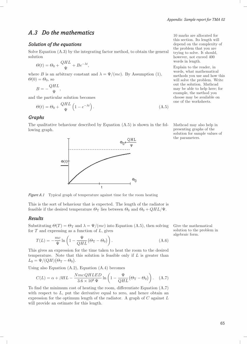
Appendix: Sample report for TMA 02
A.3 Do the mathematics
Solution of the equationsSolve Equation (A.3) by the integrating factor method, to obtain the general
10 marks are allocated forthis section. Its length willdepend on the complexity ofthe problem that you aretrying to solve. It should,however, not exceed 400words in length.Explain to the reader, inwords, what mathematicalmethods you use and how thiswill solve the problem. Writeout the solution. Mathcadmay be able to help here; forexample, the method youchoose may be available onone of the worksheets.
solution
Θ(t) = Θ0 +QHL
Ψ+ Be−λt,
where B is an arbitrary constant and λ = Ψ/(mc). By Assumption (1),Θ(0) = Θ0, so
B = −QHL
Ψ,
and the particular solution becomes
Θ(t) = Θ0 +QHL
Ψ
(1− e−λt
). (A.5)
GraphsThe qualitative behaviour described by Equation (A.5) is shown in the fol- Mathcad may also help in
presenting graphs of thesolution for sample values ofthe parameters.
lowing graph.
Figure A.1 Typical graph of temperature against time for the room heating
This is the sort of behaviour that is expected. The length of the radiator isfeasible if the desired temperature ΘT lies between Θ0 and Θ0 + QHL/Ψ.
ResultsSubstituting Θ(T ) = ΘT and λ = Ψ/(mc) into Equation (A.5), then solving Give the mathematical
solution to the problem inalgebraic form.
for T and expressing as a function of L, gives
T (L) = −mc
Ψln
(1− Ψ
QHL
(ΘT −Θ0
)). (A.6)
This gives an expression for the time taken to heat the room to the desiredtemperature. Note that this solution is feasible only if L is greater thanL0 = Ψ/(QH)
(ΘT −Θ0
).
Using also Equation (A.2), Equation (A.4) becomes
C(L) = α + βHL− NmcQHLED
3.6× 10⁸ Ψln
(1− Ψ
QHL
(ΘT −Θ0
)). (A.7)
To find the minimum cost of heating the room, differentiate Equation (A.7)with respect to L, put the derivative equal to zero, and hence obtain anexpression for the optimum length of the radiator. A graph of C against Lwill provide an estimate for this length.
65

Appendix: Sample report for TMA 02
A.4 Interpret the results
Data
13 marks are allocated forthis section, which should beno more than 500 words inlength.You should present the datathat you have collected,giving references to anysources of data that you haveused. If you have done yourown experiments to collectdata, then the descriptions ofthose experiments shouldappear in an appendix at theend of the report.
Quantity Value Source or justification
l 4.0m measuredw 3.2m measuredh 2.8m measuredρ 1.293 kgm−3 www.answers.com/topic/density-of-airm 46.34 kg Equation (A.1)H 0.45 m Appendix 1α 3.1£ Appendix 1β 95£m−2 Appendix 1Θ0 0 ◦C heating generally takes place only when
it is cold outsideΘT 18 ◦C generally reckoned to be a comfortable
temperaturec 993 J kg−1 K−1 MST209 Unit 15Ψ 47.85 W K−1 Appendix 2Q 2037W m−2 Appendix 1E 6.5 pence (kWh)−1 electricity billD 150 days year−1 this is just under half a yearN 15 years radiators last this long
Interpretation of resultsUsing the given data, the graph of C against L gives an estimate of the You should, if possible, give
both a qualitative andquantitative interpretation ofyour solution. The qualitativeinterpretation might includehow the solution varies withdifferent parameters andwhether this agrees withcommon sense, or it mightexamine whether the solutionbehaves as expected inlimiting cases, or in simplersituations. Choose anappropriate level of accuracyfor your numerical results.Be careful to present yoursolution in such a way that itaddresses the purpose of themathematical model.
optimum length, which is then used in a Mathcad solve block to determinethis length more accurately.
Figure A.2 Graph of total cost against length of radiator
The graph and the Mathcad solve block show that the optimum length of ra-diator is Lopt = 1.33m. The corresponding value of T , from Equation (A.6),is T (Lopt) = 1184 seconds, so according to the model it takes approximately20 minutes to warm the room up from 0 ◦C to 18 ◦C. The cost of doing sofor 150 days per year over 15 years is approximately £118.
The radiator can only heat up the room to the desired temperature if L isgreater than 0.94 m.
To test the sensitivity of the results to small changes in the parameters,change a selection of the parameters by 10%. The table below gives theparameter changes and the percentage change in the value of Lopt resultingfrom each of these parameter changes.
66

Appendix: Sample report for TMA 02
Sensitivity of Lopt to a 10% increase in parameter value
Parameter Symbol Lopt Change in Lopt Change (%)
energy cost E 1.354 0.026 2.0mass of air m 1.354 0.026 2.0days per year D 1.354 0.026 2.0number of years N 1.354 0.026 2.0heat loss rate K−1 Ψ 1.432 0.105 7.9desired temperature ΘT 1.460 0.133 10.0height of room H 1.206 −0.121 −9.1
The conclusion is that the optimum length is not unduly sensitive to changesin these parameter values, since in each case the percentage variation is nomore than the 10% change in the parameter.
Choice of results to compare with realityTest the validity of Equations (A.5) and (A.6) by comparing the modelled Which of your results can be
tested against reality? Thesetests do not have to bedirectly related to the purposeof the model, and there maybe ways of testing thereliability of your model byusing it to make predictionsin simple situations, or onlyfor parts of the model.
results with those of a simple experiment involving heating a room. Thedetails of the experiment are given in Appendix 3. Test the validity of Equa-tion (A.2) by looking at the costs of buying radiators (see Appendix 1). Testthe validity of Assumption (7) by looking at the heat output for various ra-diators (see Appendix 1).
A.5 Evaluate the model
Comparison with realityA graph of Θ against t for the model and chosen data is shown below. A
17 marks are allocated forthis section, which should beabout 400 words in length.You should try to comparesome of the predictions ofyour model with real data, inorder to test the model’saccuracy and reliability.Again, you should givereferences to any sources ofdata, and if you have carriedout any experiments then youshould present your resultshere. The descriptions of theexperiments can be put in anappendix at the end of thereport. How reliable are yourresults? Are any of thesimplifications that you madelikely to have led to an answerthat is too large or too small?If you feel that there are noappropriate tests for yourmodel, then you shouldexplain why.
comparison with the graph in Appendix 3 suggests qualitative agreement,but that the values of certain parameters may not be accurate.
Figure A.3 Graph of temperature against time for chosen data
From the results of Appendix 3, the most serious deficiencies in the modelarise from Assumption (2), which will give too small a value for the heatcapacity of the room, and Assumption (3), since there will be significantheat losses through the internal walls, doors, ceiling and floor.
67
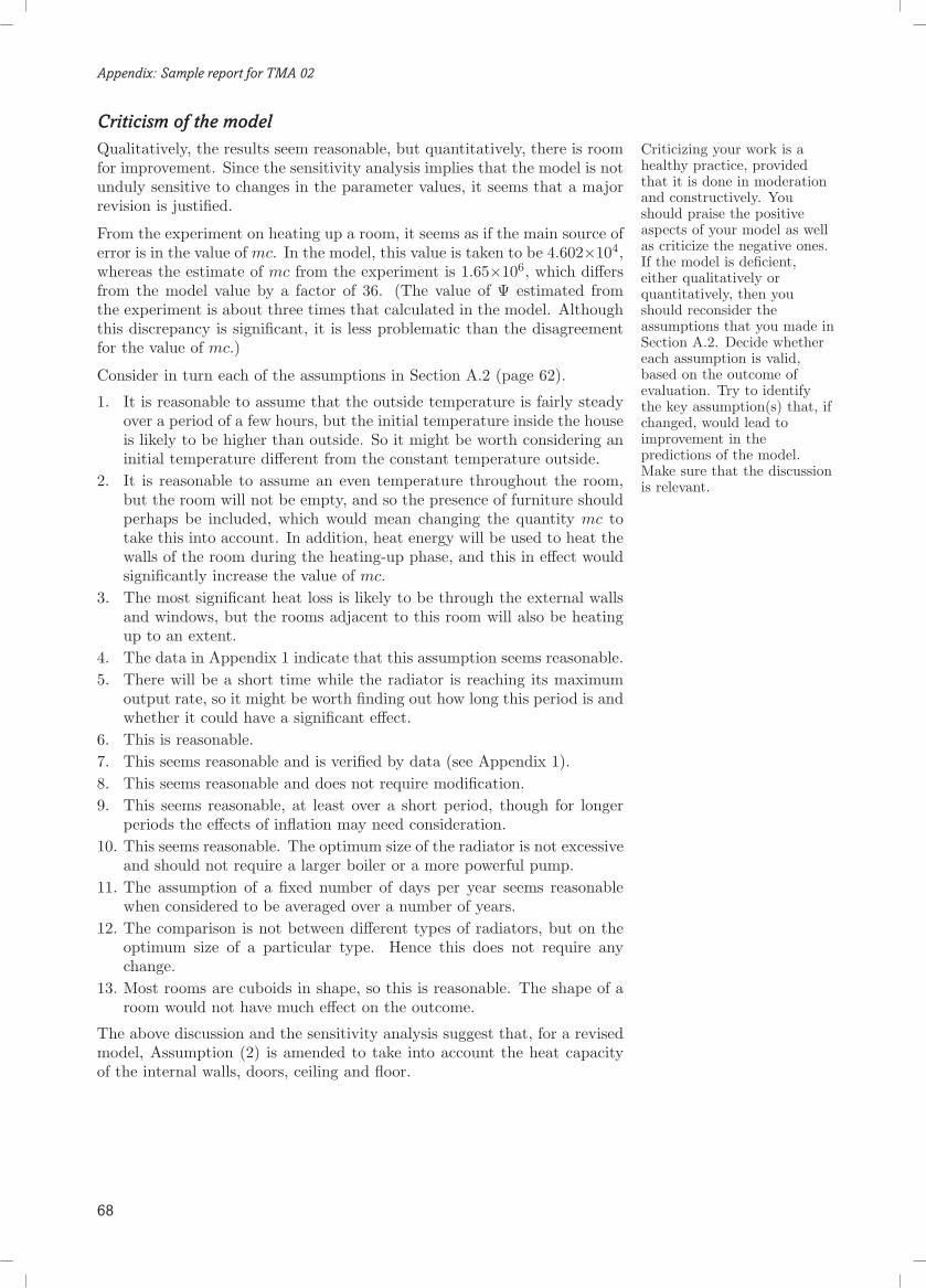
Appendix: Sample report for TMA 02
Criticism of the modelQualitatively, the results seem reasonable, but quantitatively, there is room Criticizing your work is a
healthy practice, providedthat it is done in moderationand constructively. Youshould praise the positiveaspects of your model as wellas criticize the negative ones.If the model is deficient,either qualitatively orquantitatively, then youshould reconsider theassumptions that you made inSection A.2. Decide whethereach assumption is valid,based on the outcome ofevaluation. Try to identifythe key assumption(s) that, ifchanged, would lead toimprovement in thepredictions of the model.Make sure that the discussionis relevant.
for improvement. Since the sensitivity analysis implies that the model is notunduly sensitive to changes in the parameter values, it seems that a majorrevision is justified.
From the experiment on heating up a room, it seems as if the main source oferror is in the value of mc. In the model, this value is taken to be 4.602×10⁴,whereas the estimate of mc from the experiment is 1.65×10⁶, which differsfrom the model value by a factor of 36. (The value of Ψ estimated fromthe experiment is about three times that calculated in the model. Althoughthis discrepancy is significant, it is less problematic than the disagreementfor the value of mc.)
Consider in turn each of the assumptions in Section A.2 (page 62).
1. It is reasonable to assume that the outside temperature is fairly steadyover a period of a few hours, but the initial temperature inside the houseis likely to be higher than outside. So it might be worth considering aninitial temperature different from the constant temperature outside.
2. It is reasonable to assume an even temperature throughout the room,but the room will not be empty, and so the presence of furniture shouldperhaps be included, which would mean changing the quantity mc totake this into account. In addition, heat energy will be used to heat thewalls of the room during the heating-up phase, and this in effect wouldsignificantly increase the value of mc.
3. The most significant heat loss is likely to be through the external wallsand windows, but the rooms adjacent to this room will also be heatingup to an extent.
4. The data in Appendix 1 indicate that this assumption seems reasonable.5. There will be a short time while the radiator is reaching its maximum
output rate, so it might be worth finding out how long this period is andwhether it could have a significant effect.
6. This is reasonable.7. This seems reasonable and is verified by data (see Appendix 1).8. This seems reasonable and does not require modification.9. This seems reasonable, at least over a short period, though for longer
periods the effects of inflation may need consideration.10. This seems reasonable. The optimum size of the radiator is not excessive
and should not require a larger boiler or a more powerful pump.11. The assumption of a fixed number of days per year seems reasonable
when considered to be averaged over a number of years.12. The comparison is not between different types of radiators, but on the
optimum size of a particular type. Hence this does not require anychange.
13. Most rooms are cuboids in shape, so this is reasonable. The shape of aroom would not have much effect on the outcome.
The above discussion and the sensitivity analysis suggest that, for a revisedmodel, Assumption (2) is amended to take into account the heat capacityof the internal walls, doors, ceiling and floor.
68

Appendix: Sample report for TMA 02
A.6 Revise the model
Description of the revisionRevise the model to take into account the heat energy needed to heat up
10 marks are allocated forthis section, which should be300–500 words in length.Your best policy for revisingand improving your model isto relax one (and no more) ofthe simplifying assumptionsthat you made in Section A.2and evaluated in Section A.5.In writing this section, youneed to make clear whichassumption has been changed.You do not need to solve therevised model, but you doneed to follow through thechanges to the formulation ofyour first model that occur asa consequence of the newassumptions.You should make aqualitative assessment of theeffects of the change to themodel that result.Note that using your firstmodel again with a new set ofvalues for the parametersdoes not constitute a revisionto the model. The revisionneeds to be based on a changein the assumptions thatunderpin the first model.After changing anassumption, you will probablyneed to modify the work thatyou did in creating the firstmodel.
the walls, doors, ceiling and floor, by adding two assumptions.
14. During the heating-up phase, heat energy is required to bring the tem-perature of the walls, doors, ceiling and floor up to the average of theinternal and external temperatures.
15. The walls, doors, ceiling, and floor all have the same specific heat ca-pacity.
The effect of this revision will be equivalent to increasing the value of mcin Equation (A.6), which will increase the value of T (L) and increase theoptimum length of the radiator.
The revised modelValues for the total mass of the walls, doors, ceiling and floor and for theirspecific heat capacity are required. For each wall/ceiling/floor, assume thatonly the interior half is heated up to temperature ΘT by the radiator beingmodelled, since the exterior half is either external (and remaining at thetemperature outside) or is being heated by a radiator in an adjoining room.
Definitions of additional variables
Symbol Description Unit
M mass of room surroundings kgcroom specific heat of the walls, doors, floor and ceiling J kg−1 K−1
The mass of the interior halves is 0.5M , where M is calculated in Appendix 4as approximately 15 570 kg. An estimate of the specific heat capacity croom
of the walls, doors, ceiling and floor is based (using Assumption (15)) on anaggregate value of 800 J kg−1 K−1. The value of Mcroom = 1.25× 10⁷ dwarfsthe value of mc = 4.60× 10⁴ for the air in the room.
The only change to the derivation is in the expression for the accumulation,which now becomes
accumulation = (mc + 0.5Mcroom)(Θ(t + δt)−Θ(t)
).
Since the rest of the development of the model is the same as before, usethe first model with mc replaced by mc + 0.5Mcroom.
A.7 Conclusions
The model shows that there is an optimum length of radiator, and derives
5 marks are allocated for thissection, which should beabout 100 words in length.This is your opportunity tosum up the work that youhave done, to say whether youhave obtained a satisfactorysolution to the problem thatyou set out to solve, and toindicate how you mightfurther improve your model.
a condition for the length of radiator that will minimize the running costsover a given number of years.
The predicted temperature changes from the first model are qualitatively,but not quantitatively, supported by comparison with reality. The mainproblem with the model seems to be the difficulty in estimating the heatlosses and the heat capacity of the room, and the revision to the modeladdressed this issue.
69
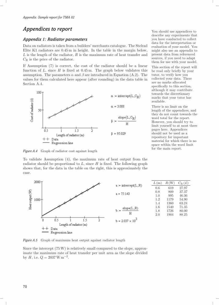
Appendix: Sample report for TMA 02
Appendices to report
Appendix 1: Radiator parametersData on radiators is taken from a builders’ merchants catalogue. The Stelrad
You should use appendices todescribe any experiments thatyou have conducted to collectdata for the interpretation orevaluation of your model. Youmight also use an appendix topresent data from referencedsources, if you need to adaptthem for use with your model.This section of the report willbe read only briefly by yourtutor, to verify how youcollected your data. Thereare no marks allocatedspecifically to this section,although it may contributetowards the discretionarymarks that your tutor hasavailable.There is no limit on thelength of the appendices, andthey do not count towards theword total for the report.However, you should try tolimit yourself to at most threepages here. Appendicesshould not be used as arepository for importantmaterial for which there is nospace within the word limitfor the main report.
L (m) R (W) CR (£)0.6 619 27.970.8 809 37.371.0 995 46.361.2 1179 54.901.4 1360 63.241.6 1540 71.351.8 1726 80.002.0 1904 88.25
Elite K1 radiators are 0.45 m in height. In the table in the margin below,L is the length of the radiator, R is the maximum rate of heat transfer andCR is the price of the radiator.
If Assumption (7) is correct, the cost of the radiator should be a linearfunction of L, since H is fixed at 0.45 m. The graph below validates thisassumption. The parameters α and β are introduced in Equation (A.2). Thevalues for them calculated here appear (after rounding) in the data table inSection A.4.
Figure A.4 Graph of radiator cost against length
To validate Assumption (4), the maximum rate of heat output from theradiator should be proportional to L, since H is fixed. The following graphshows that, for the data in the table on the right, this is approximately thecase.
Figure A.5 Graph of maximum heat output against radiator length
Since the intercept (75W) is relatively small compared to the slope, approx-imate the maximum rate of heat transfer per unit area as the slope dividedby H , i.e. Q = 2037 W m−2.
70

Appendix: Sample report for TMA 02
Appendix 2: Room dataThe room is on the corner of the building, on the ground floor, with twooutside walls and one window. There is a cellar below the room and abedroom above it. The outside walls are made of solid brick, for which theU -value is estimated as 2.1 W m−2 K−1. The window has a wooden frameand is single-glazed, for which the U -value is estimated as 5.0 W m−2 K−1.The window is 1m wide and 1.9 m high. The room is 2.8 m high, and 3.2 mby 4.0 m in plan area.
Component Area U -value UA
window 1× 1.9 = 1.9 5.0 9.5walls 2.8× (3.2 + 4.0)− 1.9 = 18.26 2.1 38.346
Hence the value of Ψ is 9.5 + 38.346 = 47.846 W K−1.
Appendix 3: Validation of model for heatingAn experiment was carried out to find the variation of temperature when theroom was heated. A 1 kW electric heater was switched on in the room, andthe temperature of the room was measured with a good thermometer, placedin the centre of the room, during the course of the day. The temperature ofthe room was initially the same as the temperature outside, which was 10◦C.The time th was measured in hours and the temperature Θ in ◦C. Themeasurements of time and temperature of the room are given in the tableon the right.
th (hours) Θ (◦C)0.25 10.00.75 10.61.17 11.31.50 12.12.08 12.72.42 13.03.25 13.83.75 14.34.33 14.64.75 15.05.50 15.16.50 15.37.67 15.78.25 15.8
10.00 16.0
The corresponding graph is shown below.
Figure A.6 Graph of temperature of room against time
Equation (A.5) from the model gives
Θ(t) = Θ0 +R
Ψ(1− e−λt
),
where λ = Ψ/(mc) and R (= 1000 W) takes the place of QHL. To validatethis model, an estimate is needed for the eventual steady-state value ofthe temperature, Θmax = Θ0 + R/Ψ. The solution can then be written asΘ(t) = Θmax − (R/Ψ)e−λt, which is equivalent to
ln(Θmax −Θ(t)
)= ln
(R
Ψ
)− λt.
71
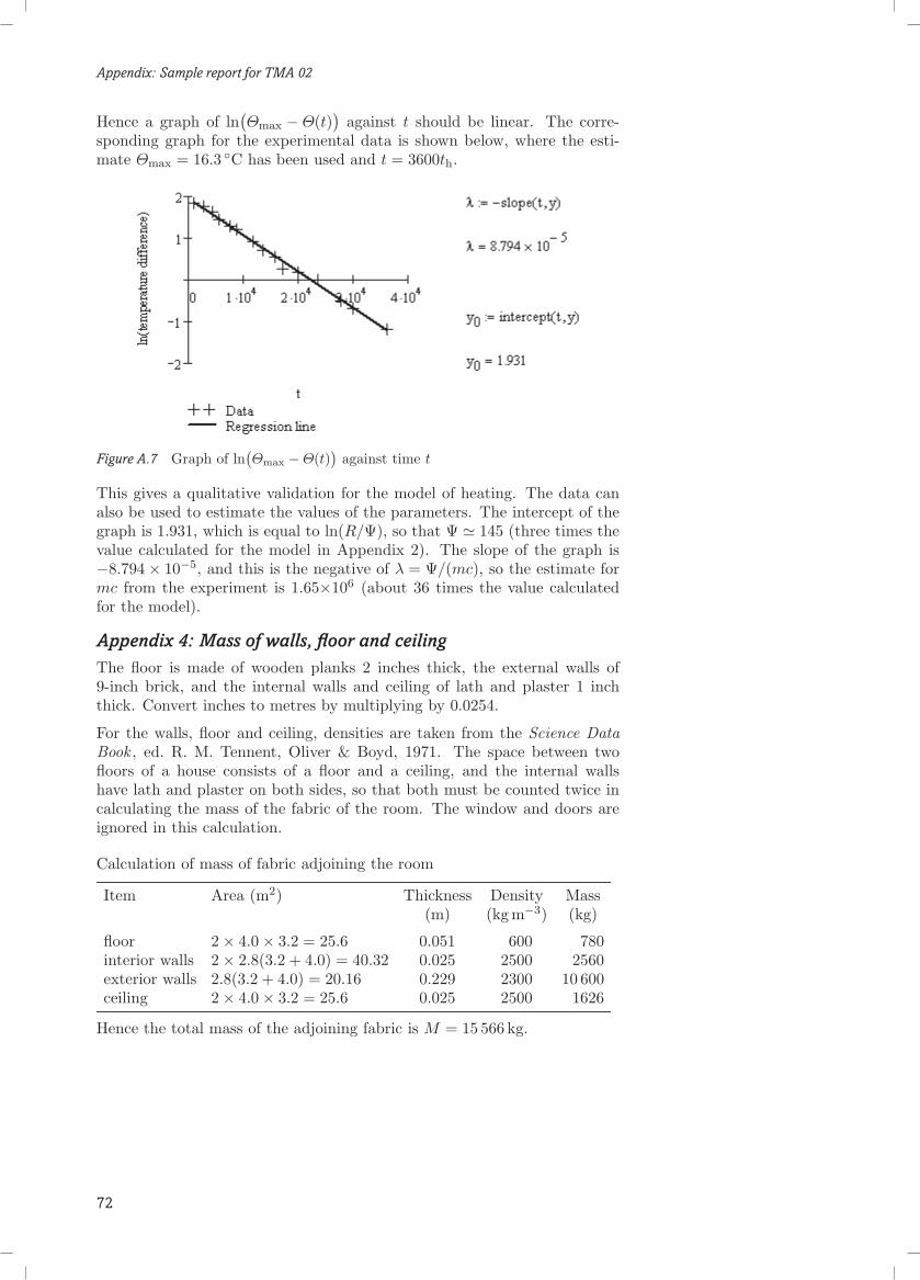
Appendix: Sample report for TMA 02
Hence a graph of ln(Θmax − Θ(t)
)against t should be linear. The corre-
sponding graph for the experimental data is shown below, where the esti-mate Θmax = 16.3 ◦C has been used and t = 3600th.
Figure A.7 Graph of ln(Θmax −Θ(t)
)against time t
This gives a qualitative validation for the model of heating. The data canalso be used to estimate the values of the parameters. The intercept of thegraph is 1.931, which is equal to ln(R/Ψ), so that Ψ / 145 (three times thevalue calculated for the model in Appendix 2). The slope of the graph is−8.794× 10⁻⁵, and this is the negative of λ = Ψ/(mc), so the estimate formc from the experiment is 1.65×10⁶ (about 36 times the value calculatedfor the model).
Appendix 4: Mass of walls, floor and ceilingThe floor is made of wooden planks 2 inches thick, the external walls of9-inch brick, and the internal walls and ceiling of lath and plaster 1 inchthick. Convert inches to metres by multiplying by 0.0254.
For the walls, floor and ceiling, densities are taken from the Science DataBook , ed. R. M. Tennent, Oliver & Boyd, 1971. The space between twofloors of a house consists of a floor and a ceiling, and the internal wallshave lath and plaster on both sides, so that both must be counted twice incalculating the mass of the fabric of the room. The window and doors areignored in this calculation.
Calculation of mass of fabric adjoining the room
Item Area (m2) Thickness Density Mass(m) (kgm−3) (kg)
floor 2× 4.0× 3.2 = 25.6 0.051 600 780interior walls 2× 2.8(3.2 + 4.0) = 40.32 0.025 2500 2560exterior walls 2.8(3.2 + 4.0) = 20.16 0.229 2300 10 600ceiling 2× 4.0× 3.2 = 25.6 0.025 2500 1626
Hence the total mass of the adjoining fabric is M = 15 566 kg.
72

Solutions to the exercises
Solutions to the exercisesSection 3
3.1 (a) Independent variable x, dependent variable y,first-order, non-linear.
(b) Independent variable s, dependent variable x,second-order, linear, not constant-coefficient, inhomo-geneous.
(c) Independent variable x, dependent variable p, first-order, linear, not constant-coefficient, inhomogeneous.
(d) Independent variable y, dependent variable p,third-order, linear, constant-coefficient, inhomoge-neous.
(e) Independent variable r, dependent variable p, first-order, linear, not constant-coefficient, inhomogeneous.
(f) Independent variable s, dependent variable q,second-order, linear, constant-coefficient, homogeneous.
3.2 (a) The differential equationdy
dx= 2xy (y > 0)
can be solved by separating variables and integrating,to obtain∫
1y
dy =∫
2xdx.
This gives ln y = x2 + C, since y > 0. This is an ac-ceptable way of writing the general solution, but theexplicit form y = function of x, if this can be achieved,is usually better. Taking exponentials of both sides,
y = exp(x2 + C) = ex2eC = Aex2
, where A = eC .
(b) The general solution is y = Aex2. Now y = 2 when
x = 0, hence A = 2. So the particular solution is
y = 2ex2.
3.3 (a) The differential equation
s2 ds
dt− s sin t = 0
can be rearranged (for s += 0) as
sds
dt= sin t,
where the variables are separated. Integrating with re-spect to t (the independent variable) gives
12s2 = − cos t + C.
(Note that s = 0 is a further solution of the given dif-ferential equation.)Using the initial condition, s(π
2 ) = −2, gives12 (−2)2 = − cos(π
2 ) + C
and therefore C = 2. The solution is12s2 = − cos t + 2.
To express s explicitly in terms of t, multiply by 2 andtake the square root (the negative square root, since theinitial condition has a negative value for s), to obtain
s = −√4− 2 cos t.
(Note that here, and in the other parts of this exer-cise, an alternative strategy is to express the dependentvariable explicitly in terms of the independent variablebefore imposing the initial condition.)
(b) The differential equation
(x2 + 1)dy
dx= xy
can be rearranged as1y
dy
dx=
x
x2 + 1(y += 0),
in which the variables are separated. Since x2 + 1 > 0and y = 1 > 0 initially, integration gives
ln y = 12 ln(x2 + 1) + C.
Now y = 1 when x = 1, so C = − 12 ln 2. Substitute this
value above, to obtainln y = 1
2 ln(x2 + 1)− 12 ln 2.
To express y explicitly, start by taking exponentials ofboth sides:
y = exp(
12 ln(x2 + 1)− 1
2 ln 2)
= exp(ln
((x2 + 1)1/2
)− ln(21/2
))= exp
(ln
(√x2 + 1√
2
))=√
x2 + 1√2
=
√x2 + 1
2.
The solution is
y =
√x2 + 1
2.
(Note the manipulations of logarithms that were neededbefore the use of exp(ln w) = w.)
(c) The differential equation
2sdp
ds= 4p− 8
can be rearranged as1
2p− 4dp
ds=
1s
(s += 0, p += 2).
Since s = 2 and p = 0 initially, so s > 0 and 2p− 4 < 0,integration gives
12 ln(4− 2p) = ln s + C.
The initial condition, p(2) = 0, gives 12 ln 4 = ln 2 + C
and therefore C = 12 ln 4− ln 2 = 0. The solution is
12 ln(4− 2p) = ln s,
which can be rearranged asp = 2− 1
2s2.
(d) The differential equation
2sdp
ds= 4p− 8
can be rearranged as1
2p− 4dp
ds=
1s
(s += 0, p += 2).
Since s = 2 and p = 4 initially, so s > 0 and 2p− 4 > 0,integration gives
12 ln(2p− 4) = ln s + C.
73

Solutions to the exercises
The initial condition, p(2) = 4, gives 12 ln 4 = ln 2 + C
and therefore C = 12 ln 4− ln 2 = 0. The solution is
12 ln(2p− 4) = ln s,
which can be rearranged asp = 1
2s2 + 2.
(e) The differential equation
xdx
dt= x3e−3t
can be rearranged as
x−2 dx
dt= e−3t (x += 0).
Integration gives−x−1 = − 1
3e−3t + C.
Now x = 1 when t = 0, so −1−1 = − 13e−0 + C and
therefore C = −1 + 13 = − 2
3 . The solution is
−x−1 = − 13e−3t − 2
3 ,
which can be rearranged as
x =3
e−3t + 2.
3.4 Rewriting the differential equationdy
dx= 4− 2y
in the standard form givesdy
dx+ 2y = 4.
The differential equation is linear, with integrating fac-tor
p(x) = exp(∫
2 dx
)= e2x.
Multiplying the standard form of differential equationby the integrating factor, and then integrating bothsides, results in
e2xy =∫
4e2x dx,
which givese2xy = 2e2x + C,
or equivalently,y = 2 + Ce−2x.
3.5 (a) First write the differential equation in stan-dard form (which can be done since x ≥ 1 > 0), as
dy
dx+
2x
y = 4x.
The differential equation is linear, with integrating fac-tor
p(x) = exp(∫
2x
dx
)= exp(2 ln x) = exp(ln x2) = x2.
Multiplying the standard form of the differential equa-tion by the integrating factor, and then integrating bothsides, results in
x2y =∫
4x3 dx,
which leads to x2y = x4 + C. Now y = 2 when x = 1,so 2 = 1 + C, which gives C = 1.
Hence x2y = x4 + 1, or equivalently,
y = x2 +1x2
.
(Note that here, and in the other parts of this exer-cise, an alternative strategy is to express the dependentvariable explicitly in terms of the independent variablebefore imposing the initial condition.)
(b) The standard form of the differential equation isdy
dx+
( −x
x2 + 1
)y = 0.
The differential equation is linear, with integrating fac-tor
p(x) = exp(∫ −x
x2 + 1dx
)= exp
(− 12 ln(x2 + 1)
)= (x2 + 1)−1/2.
Multiplying the standard form of the differential equa-tion by the integrating factor, and then integrating bothsides, results in
(x2 + 1)−1/2y =∫
0 dx,
which leads to (x2 + 1)−1/2y = C, or equivalently,
y = C(x2 + 1)1/2.
Now y = 1 when x = 1, so 1 = C(12 + 1)1/2, which givesC = 2−1/2. The solution is
y = 2−1/2(x2 + 1)1/2 =
√x2 + 1
2,
as also found in Solution 3.3(b).
(c) The standard form of the differential equation isdx
dt+
5tx = 7t + 4t−2.
The differential equation is linear, with integrating fac-tor (since t ≥ 1)
p(t) = exp(∫
5t
dt
)= e5 ln t = eln(t5) = t5.
Multiplying the standard form of the differential equa-tion by the integrating factor, and then integrating bothsides, results in
t5x =∫
(7t6 + 4t3) dt,
which leads tot5x = t7 + t4 + C.
Now x = 4 when t = 1, so 154 = 17 + 14 + C, whichgives C = 2. The solution is t5x = t7 + t4 + 2, or equiv-alently,
x = t2 + t−1 + 2t−5.
3.6 For 3x + 12x = 6, the associated homogeneous dif-ferential equation is
3x + 12x = 0.
This has the auxiliary equation 3λ2 + 12 = 0, with roots±2i, so the complementary function is
x = A cos(2t) + B sin(2t) (or C cos(2t + φ)) .
For the particular integral try x = c, where c is a con-stant, so x = x = 0. Substitution into the original dif-ferential equation gives 12c = 6 or c = 1
2 .
74

Solutions to the exercises
The general solution is thereforex = A cos(2t) + B sin(2t) + 1
2
(or C cos(2t + φ) + 1
2
).
(If you are unfamiliar with some of the words used here,then read the explanation in the text after this exercise.)
3.7 (a) The auxiliary equation is3λ− 4 = 0,
and therefore λ = 43 . The general solution is
y = Ce4x/3.
(b) The auxiliary equation is2λ + 5 = 0,
and therefore λ = − 52 . The general solution is
y = Ce−5t/2.
(c) The auxiliary equation is
λ2 + 3λ− 4 = (λ− 1)(λ + 4) = 0,
so λ1 = 1, λ2 = −4. The general solution isy = Cex + De−4x.
(d) The auxiliary equation is
λ2 − 4λ + 4 = (λ− 2)2 = 0,
so λ1 = λ2 = 2. The general solution isx = (C + Dt)e2t.
(e) The auxiliary equation is
λ2 + 2λ + 5 = 0,
so λ = 12
(−2±√4− 20)
= −1± 2i. The general solu-tion is
y = e−x(C cos(2x) + D sin(2x)
).
(f) The auxiliary equation is
λ2 − 4λ = λ(λ− 4) = 0,
so λ1 = 0, λ2 = 4. The general solution isy = Ce0 + De4t = C + De4t.
(g) The auxiliary equation is
λ2 − 4 = 0,
so λ = ±2. The general solution isy = Ce2x + De−2x.
(h) The auxiliary equation is
λ2 + 4 = 0,
so λ = ±2i. The general solution isx = C cos(2t) + D sin(2t).
3.8 (a) From Solution 3.7(b), the complementaryfunction is
yc = Ce−5t/2.
For a particular integral, try a function of the formy = p1t + p0,
so dy/dt = p1. Substituting into the differential equa-tion leads to
2p1 + 5(p1t + p0) = 10t,
which, upon equating coefficients, gives p1 = 2 andp0 = − 4
5 . So a particular integral is
yp = 2t− 45 .
The general solution is
y = Ce−5t/2 + 2t− 45 .
(Notice that, even though the right-hand side of thedifferential equation has no constant term, you need toinclude a constant term in the trial solution.)
(b) From Solution 3.7(b), the complementary functionis
yc = Ce−5t/2.
For a particular integral, try a function of the formy = pe−2t,
so dy/dt = −2pe−2t. Substituting into the differentialequation leads to
2(−2pe−2t
)+ 5
(pe−2t
)= 3e−2t,
which gives p = 3. So a particular integral isyp = 3e−2t.
The general solution is
y = Ce−5t/2 + 3e−2t.
(c) From Solution 3.7(b), the complementary functionis
yc = Ce−5t/2.
For a particular integral, try a function of the formy = p cos(2t) + q sin(2t),
so dy/dt = −2p sin(2t) + 2q cos(2t). Substituting intothe differential equation leads to
2(−2p sin(2t) + 2q cos(2t)
)+ 5
(p cos(2t) + q sin(2t)
)= sin(2t),
which, upon equating coefficients, gives−4p + 5q = 1,
5p + 4q = 0,
for which the solution is p = − 441 and q = 5
41 . So aparticular integral is
yp = − 441 cos(2t) + 5
41 sin(2t).The general solution is
y = Ce−5t/2 − 441 cos(2t) + 5
41 sin(2t).
(d) From Solution 3.7(c), the complementary functionis
yc = Cex + De−4x.
To find a particular integral, try a function of the formy = pe2x,
so dy/dx = 2pe2x and d2y/dx2 = 4pe2x. Substitutinginto the differential equation leads to
(4pe2x) + 3(2pe2x)− 4(pe2x) = 2e2x,
i.e. 6pe2x = 2e2x, which gives p = 13 . So a particular
integral isyp = 1
3e2x.
The general solution isy = Cex + De−4x + 1
3e2x.
75
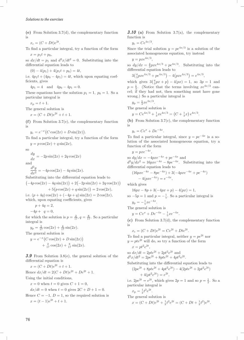
Solutions to the exercises
(e) From Solution 3.7(d), the complementary functionis
xc = (C + Dt)e2t.
To find a particular integral, try a function of the formx = p1t + p0,
so dx/dt = p1 and d2x/dt2 = 0. Substituting into thedifferential equation leads to
(0)− 4(p1) + 4(p1t + p0) = 4t,
i.e. 4p1t + (4p0 − 4p1) = 4t, which upon equating coef-ficients, gives
4p1 = 4 and 4p0 − 4p1 = 0.
These equations have the solution p1 = 1, p0 = 1. So aparticular integral is
xp = t + 1.
The general solution isx = (C + Dt)e2t + t + 1.
(f) From Solution 3.7(e), the complementary functionis
yc = e−x(C cos(2x) + D sin(2x)
).
To find a particular integral, try a function of the formy = p cos(2x) + q sin(2x),
sody
dx= −2p sin(2x) + 2q cos(2x)
andd2y
dx2= −4p cos(2x)− 4q sin(2x).
Substituting into the differential equation leads to(−4p cos(2x)− 4q sin(2x))
+ 2(−2p sin(2x) + 2q cos(2x)
)+ 5
(p cos(2x) + q sin(2x)
)= 2 cos(2x),
i.e. (p + 4q) cos(2x) + (−4p + q) sin(2x) = 2 cos(2x),which, upon equating coefficients, gives
p + 4q = 2,
−4p + q = 0,
for which the solution is p = 217 , q = 8
17 . So a particularintegral is
yp = 217 cos(2x) + 8
17 sin(2x).The general solution is
y = e−x(C cos(2x) + D sin(2x)
)+ 2
17 cos(2x) + 817 sin(2x).
3.9 From Solution 3.8(e), the general solution of thedifferential equation is
x = (C + Dt)e2t + t + 1.
Hence dx/dt = 2(C + Dt)e2t + De2t + 1.Using the initial conditions,
x = 0 when t = 0 gives C + 1 = 0,
dx/dt = 0 when t = 0 gives 2C + D + 1 = 0.
Hence C = −1, D = 1, so the required solution isx = (t− 1)e2t + t + 1.
3.10 (a) From Solution 3.7(a), the complementaryfunction is
yc = Ce4x/3.
Since the trial solution y = pe4x/3 is a solution of theassociated homogeneous equation, try instead
y = pxe4x/3,
so dy/dx = 43pxe4x/3 + pe4x/3. Substituting into the
differential equation leads to
3(
43pxe4x/3 + pe4x/3
)− 4(pxe4x/3
)= e4x/3,
which gives 3(
43px + p
) − 4(px) = 1, so 3p = 1 andp = 1
3 . (Notice that the terms involving xe4x/3 can-cel; if they had not, then something must have gonewrong.) So a particular integral is
yp = 13xe4x/3.
The general solution is
y = Ce4x/3 + 13xe4x/3 =
(C + 1
3x)e4x/3.
(b) From Solution 3.7(c), the complementary functionis
yc = Cex + De−4x.
To find a particular integral, since y = pe−4x is a so-lution of the associated homogeneous equation, try afunction of the form
y = pxe−4x,
so dy/dx = −4pxe−4x + pe−4x andd2y/dx2 = 16pxe−4x − 8pe−4x. Substituting into thedifferential equation leads to
(16pxe−4x − 8pe−4x) + 3(−4pxe−4x + pe−4x)− 4(pxe−4x) = e−4x,
which gives16px− 8p + 3(−4px + p)− 4(px) = 1,
so −5p = 1 and p = − 15 . So a particular integral is
yp = − 15xe−4x.
The general solution isy = Cex + De−4x − 1
5xe−4x.
(c) From Solution 3.7(d), the complementary functionis
xc = (C + Dt)e2t = Ce2t + Dte2t.
To find a particular integral, neither y = pe2t nory = pte2t will do, so try a function of the form
x = pt2e2t,
so dx/dt = 2pte2t + 2pt2e2t andd2x/dt2 = 2pe2t + 8pte2t + 4pt2e2t.Substituting into the differential equation leads to
(2pe2t + 8pte2t + 4pt2e2t)− 4(2pte2t + 2pt2e2t)+ 4(pt2e2t) = e2t,
i.e. 2pe2t = e2t, which gives 2p = 1 and so p = 12 . So a
particular integral isxp = 1
2 t2e2t.
The general solution isx = (C + Dt)e2t + 1
2 t2e2t = (C + Dt + 12 t2)e2t.
76

Solutions to the exercises
3.11 The augmented matrix is:
A|b =
1 3 −2 33 7 3 165 3 −2 11
R1
R2
R3
Stage 1 : eliminationStage 1(a): first column
R2 − 3R1
R3 − 5R1
1 3 −2 30 −2 9 70 −12 8 −4
R1
R2a
R3a
Stage 1(b): second column
R3a − 6R2a
1 3 −2 30 −2 9 70 0 −46 −46
R1
R2a
R3b
The matrix A is now in upper triangular form, and thesolution can be obtained by back substitution.Stage 2 : back substitutionThe third row gives −46x3 = −46, so x3 = 1. The sec-ond row gives −2x2 + 9x3 = 7, so x2 = 1. The first rowgives x1 + 3x2 − 2x3 = 3, so x1 = 2. In matrix terms,the solution is x = [2 1 1]T .
3.12 (a) The augmented matrix is:
A|b =
2 3 −2 14 6 3 26 3 −2 9
R1
R2
R3
Stage 1 : eliminationStage 1(a): first column
R2 − 2R1
R3 − 3R1
2 3 −2 10 0 7 00 −6 4 6
R1
R2a
R3a
Stage 1(b): second column. The pivot for stage 1(b)is zero, so it is necessary to perform an essential rowinterchange. Interchanging R2a and R3a gives
R3a ↔ R2a
2 3 −2 10 −6 4 60 0 7 0
R1
R2b
R3b
Stage 2 : back substitutionThe third row gives 7x3 = 0, so x3 = 0. The second rowgives −6x2 + 4x3 = 6, so x2 = −1. The first row gives2x1 + 3x2 − 2x3 = 1, so x1 = 2. Hence the solution isx = [2 − 1 0]T .
(b) The augmented matrix is:
A|b =
2 3 −2 14 6 3 26 9 −2 3
R1
R2
R3
Stage 1 : eliminationStage 1(a): first column
R2 − 2R1
R3 − 3R1
2 3 −2 10 0 7 00 0 4 0
R1
R2a
R3a
The matrix is already in upper triangular form, sostage 1 is complete.Stage 2 : back substitutionThe third row gives 4x3 = 0, so x3 = 0. The second row
gives 7x3 = 0, therefore x2 can take any value. Takex2 = k. The first row gives 2x1 + 3x2 − 2x3 = 1, sox1 = 1
2 (1 − 3k). Hence, there is an infinite number ofsolutions of the form x = [ 12 (1− 3k) k 0]T .
(c) The augmented matrix is:
A|b =
2 3 −2 14 6 3 26 9 −2 7
R1
R2
R3
Stage 1 : eliminationStage 1(a): first column
R2 − 2R1
R3 − 3R1
2 3 −2 10 0 7 00 0 4 4
R1
R2a
R3a
Again, the matrix is already in upper triangular form,so stage 1 is complete.Stage 2 : back substitutionThe third row gives 4x3 = 4, so x3 = 1. The second rowgives 7x3 = 0, so x3 = 0. Since these two results are in-consistent, the system of equations has no solution.∣∣∣∣ 4 1
1 2
∣∣∣∣ = 4× 2− 1× 1 = 7.3.13 (a)∣∣∣∣ 1 24 1
∣∣∣∣ = 1× 1− 2× 4 = −7.(b)
(Interchanging two rows of a determinant changes thesign of the determinant.)∣∣∣∣∣∣
2 3 −24 6 36 3 −2
∣∣∣∣∣∣ = 2×∣∣∣∣ 6 33 −2
∣∣∣∣− 3×∣∣∣∣ 4 36 −2
∣∣∣∣(c)
+ (−2)×∣∣∣∣ 4 66 3
∣∣∣∣= 2× (−21)− 3× (−26)− 2× (−24)= 84.∣∣∣∣∣∣
2 3 −20 6 30 0 −2
∣∣∣∣∣∣ = 2× 6× (−2) = −24.(d)
(The determinant of an upper (or lower) triangular ma-trix is the product of the diagonal elements.)∣∣∣∣∣∣
2 3 −24 6 36 9 −2
∣∣∣∣∣∣ = 2×∣∣∣∣ 6 39 −2
∣∣∣∣− 3×∣∣∣∣ 4 36 −2
∣∣∣∣(e)
+ (−2)×∣∣∣∣ 4 66 9
∣∣∣∣= 2× (−39)− 3× (−26)− 2× 0= 0.
Only the matrix in part (e) has determinant zero, soonly this matrix is singular.(Note that the matrix from part (e) is that from Exer-cise 3.12(b) and (c). When solving a system of linearequations, when the coefficient matrix is singular, thereare either no solutions (as in Exercise 3.12(c)) or an in-finite number of solutions (as in Exercise 3.12(b)). If amatrix is non-singular, the system of linear equationsalways has a unique solution.)
77

Solutions to the exercises
3.14 The characteristic equation is∣∣∣∣−7− λ 53 −5− λ
∣∣∣∣ = 0.
Expanding the determinant gives(−7− λ)(−5− λ)− 3× 5 = λ2 + 12λ + 20 = 0.
Factorizing this equation gives(λ + 10)(λ + 2) = 0,
so the eigenvalues are −10 and −2.To find the corresponding eigenvectors, consider eacheigenvalue in turn and solve the equation(A− λI)v = 0, where v = [x y]T .
λ = −10 The eigenvector equation becomes{(−7− (−10))x + 5y = 0,
3x +(−5− (−10)
)y = 0.
Both of these equations give3x + 5y = 0,
so an eigenvector is [5 − 3]T .
λ = −2 The eigenvector equation becomes{(−7− (−2))x + 5y = 0,
3x +(−5− (−2)
)y = 0.
Both of these equations givex− y = 0,
so an eigenvector is [1 1]T .(If you are unsure about determinants, then see Sub-section 3.5. If you are unsure about finding eigenvaluesand eigenvectors, then read the explanation followingthis exercise.)
3.15 (a) The characteristic equation is∣∣∣∣ 2− λ 43 1− λ
∣∣∣∣ = 0.
Expanding the determinant gives(2− λ)(1− λ)− 3× 4 = λ2 − 3λ− 10 = 0.
(b) Factorizing the characteristic equation gives(λ− 5)(λ + 2) = 0,
so the eigenvalues are 5 and −2.
3.16 (a) The characteristic equation is(1− λ)
((−3− λ)(3− λ)− (−2)× 4
)= 0,
which reduces to(1− λ)(λ2 − 1) = (1− λ)(λ− 1)(λ + 1) = 0,
so the eigenvalues are −1 and 1 (twice).
(b) The characteristic equation is(1− λ)(1− λ)(−1− λ) = −(1− λ)2(1 + λ) = 0,
so the eigenvalues are −1 and 1 (twice).
λ = 5 k[4 3]T3.17 (a)
λ = −2 k[1 −1]T
λ = −1 k[1 2 1]T(b)
λ = 1 [k l l]T (= k[1 0 0]T + l[0 1 1]T )
λ = −1 k[0 0 1]T(c)
λ = 1 k[1 0 0]T
(d) Since the matrix is upper triangular, the eigenval-ues are 1, 2 and 3.
λ = 1 k[1 0 0]T
λ = 2 k[1 1 0]T
λ = 3 k[1 1 1]T
3.18 The characteristic equation is(−3− λ)(1− λ)− 4× (−2) = λ2 + 2λ + 5 = 0,
for which the solutions are λ = −1± 2i. One eigenvalueand corresponding eigenvectors are:
λ = −1 + 2i k[−1 1 + i]T
The complex conjugates of these give the second eigen-value and associated eigenvectors.
3.19 (a) This 3× 3 matrix, from Exercise 3.17(b), has3 linearly independent eigenvectors.
(b) This 3× 3 matrix, from Exercise 3.17(c), has only2 linearly independent eigenvectors.
3.20 First, form the associated homogeneous system[x1
x2
]=
[−7 53 −5
] [x1
x2
].
Using the trial solution[x1
x2
]= veλt,
where v is a constant vector, gives
λ2veλt =[−7 5
3 −5
]veλt,
and dividing by eλt (which is never zero) gives
λ2v =[−7 5
3 −5
]v.
The eigenvalues of the matrix give λ2 and the eigenvec-tors give v. Using Solution 3.14, the complementaryfunction is[
x1
x2
]= C1
[11
]cos
(√2t + φ1
)+ C2
[5
−3
]cos
(√10t + φ2
),
where C1, C2, φ1 and φ2 are arbitrary constants. Forthe particular integral, try[
x1
x2
]=
[c1
c2
].
On substitution, this gives[00
]=
[−7 53 −5
] [c1
c2
]+
[−37
],
whose solution is[c1
c2
]=
[12
].
78
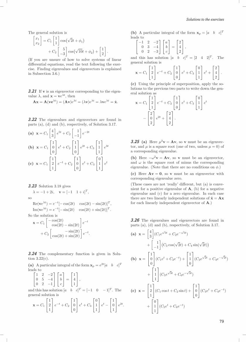
Solutions to the exercises
The general solution is[x1
x2
]= C1
[11
]cos
(√2t + φ1
)+ C2
[5
−3
]cos
(√10t + φ2
)+
[12
].
(If you are unsure of how to solve systems of lineardifferential equations, read the text following the exer-cise. Finding eigenvalues and eigenvectors is explainedin Subsection 3.6.)
3.21 If v is an eigenvector corresponding to the eigen-value λ, and x = veλt, then
Ax = A(veλt) = (Av)eλt = (λv)eλt = λveλt = x.
3.22 The eigenvalues and eigenvectors are found inparts (a), (d) and (b), respectively, of Solution 3.17.
x = C1
[43
]e5t + C2
[1
−1
]e−2t(a)
x = C1
100
et + C2
110
e2t + C3
111
e3t(b)
x = C1
121
e−t + C2
100
et + C3
011
et(c)
3.23 Solution 3.18 givesλ = −1 + 2i, v = [−1 1 + i]T ,
soRe(veλt) = e−t[− cos(2t) cos(2t)− sin(2t)]T ,
Im(veλt) = e−t[− sin(2t) cos(2t) + sin(2t)]T .
So the solution is
x = C1
[− cos(2t)cos(2t)− sin(2t)
]e−t
+ C2
[ − sin(2t)cos(2t) + sin(2t)
]e−t.
3.24 The complementary function is given in Solu-tion 3.22(c).
(a) A particular integral of the form xp = e2t[a b c]T
leads to 1 2 −20 5 −40 2 −1
abc
=
141
,
and this has solution [a b c]T = [−1 0 − 1]T . Thegeneral solution is
x = C1
121
e−t + C2
100
et + C3
011
et − 1
01
e2t.
(b) A particular integral of the form xp = [a b c]T
leads to−1 2 −20 3 −40 2 −3
abc
=
242
,
and this has solution [a b c]T = [2 4 2]T . Thegeneral solution is
x = C1
121
e−t + C2
100
et + C3
011
et +
242
.
(c) Using the principle of superposition, apply the so-lutions to the previous two parts to write down the gen-eral solution as
x = C1
121
e−t + C2
100
et + C3
011
et
− 2
02
e2t +
242
.
3.25 (a) Here µ2v = Av, so v must be an eigenvec-tor, and µ is a square root (one of two, unless µ = 0) ofa corresponding eigenvalue.
(b) Here −ω2v = Av, so v must be an eigenvector,and ω is the square root of minus the correspondingeigenvalue. (Note that there are no conditions on φ.)
(c) Here Av = 0, so v must be an eigenvector withcorresponding eigenvalue zero.(These cases are not ‘really’ different, but (a) is conve-nient for a positive eigenvalue of A, (b) for a negativeeigenvalue and (c) for a zero eigenvalue. In each casethere are two linearly independent solutions of x = Axfor each linearly independent eigenvector of A.)
3.26 The eigenvalues and eigenvectors are found inparts (a), (d) and (b), respectively, of Solution 3.17.
x =[
43
](C1e
√5t + C2e
−√5t)(a)
+[
1−1
](C3 cos(
√2t) + C4 sin(
√2t)
)x =
100
(C1et + C2e
−t) +
110
(C3e√
2t + C4e−√2t)(b)
+
111
(C5e√
3t + C6e−√3t)
x =
121
(C1 cos t + C2 sin t) +
100
(C3et + C4e
−t)(c)
+
011
(C5et + C6e
−t)
79
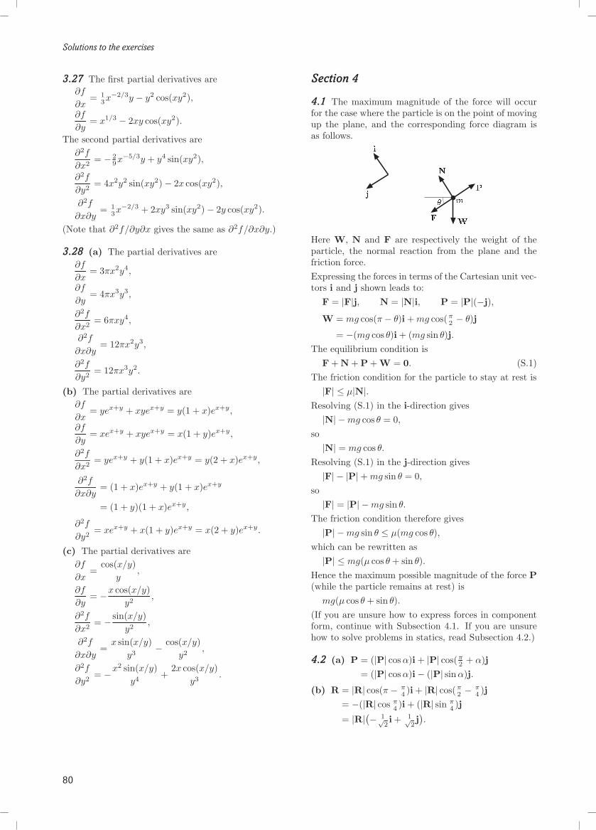
Solutions to the exercises
3.27 The first partial derivatives are∂f
∂x= 1
3x−2/3y − y2 cos(xy2),
∂f
∂y= x1/3 − 2xy cos(xy2).
The second partial derivatives are∂2f
∂x2= − 2
9x−5/3y + y4 sin(xy2),
∂2f
∂y2= 4x2y2 sin(xy2)− 2x cos(xy2),
∂2f
∂x∂y= 1
3x−2/3 + 2xy3 sin(xy2)− 2y cos(xy2).
(Note that ∂2f/∂y∂x gives the same as ∂2f/∂x∂y.)
3.28 (a) The partial derivatives are∂f
∂x= 3πx2y4,
∂f
∂y= 4πx3y3,
∂2f
∂x2= 6πxy4,
∂2f
∂x∂y= 12πx2y3,
∂2f
∂y2= 12πx3y2.
(b) The partial derivatives are∂f
∂x= yex+y + xyex+y = y(1 + x)ex+y,
∂f
∂y= xex+y + xyex+y = x(1 + y)ex+y,
∂2f
∂x2= yex+y + y(1 + x)ex+y = y(2 + x)ex+y,
∂2f
∂x∂y= (1 + x)ex+y + y(1 + x)ex+y
= (1 + y)(1 + x)ex+y,
∂2f
∂y2= xex+y + x(1 + y)ex+y = x(2 + y)ex+y.
(c) The partial derivatives are∂f
∂x=
cos(x/y)y
,
∂f
∂y= −x cos(x/y)
y2,
∂2f
∂x2= − sin(x/y)
y2,
∂2f
∂x∂y=
x sin(x/y)y3
− cos(x/y)y2
,
∂2f
∂y2= −x2 sin(x/y)
y4+
2x cos(x/y)y3
.
Section 4
4.1 The maximum magnitude of the force will occurfor the case where the particle is on the point of movingup the plane, and the corresponding force diagram isas follows.
Here W, N and F are respectively the weight of theparticle, the normal reaction from the plane and thefriction force.Expressing the forces in terms of the Cartesian unit vec-tors i and j shown leads to:
F = |F|j, N = |N|i, P = |P|(−j),
W = mg cos(π− θ)i + mg cos(π2 − θ)j
= −(mg cos θ)i + (mg sin θ)j.The equilibrium condition is
F + N + P + W = 0. (S.1)The friction condition for the particle to stay at rest is|F| ≤ µ|N|.
Resolving (S.1) in the i-direction gives|N| −mg cos θ = 0,
so|N| = mg cos θ.
Resolving (S.1) in the j-direction gives|F| − |P|+ mg sin θ = 0,
so|F| = |P| −mg sin θ.
The friction condition therefore gives|P| −mg sin θ ≤ µ(mg cos θ),
which can be rewritten as|P| ≤ mg(µ cos θ + sin θ).
Hence the maximum possible magnitude of the force P(while the particle remains at rest) is
mg(µ cos θ + sin θ).(If you are unsure how to express forces in componentform, continue with Subsection 4.1. If you are unsurehow to solve problems in statics, read Subsection 4.2.)
P = (|P| cos α)i + |P| cos(π2 + α)j4.2 (a)
= (|P| cos α)i− (|P| sin α)j.
R = |R| cos(π− π4 )i + |R| cos(π
2 − π4 )j(b)
= −(|R| cos π4 )i + (|R| sin π
4 )j
= |R|(− 1√2i + 1√
2j).
80
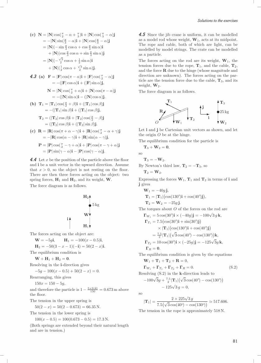
Solutions to the exercises
N = |N| cos(π2 − α + π
3 )i + |N| cos(π3 − α)j(c)
= −|N| sin(π3 − α)i + |N| cos(π
3 − α)j= |N|(− sin π
3 cosα + cos π3 sin α)i
+ |N|(cos π3 cosα + sin π
3 sin α)j
= |N|(−√
32 cos α + 1
2 sin α)i
+ |N|(12 cosα +
√3
2 sin α)j.
F = |F| cos(π− α)i + |F| cos(π2 − α)j4.3 (a)
= −(|F| cos α)i + (|F| sin α)j,
N = |N| cos(π2 + α)i + |N| cos(π− α)j
= −(|N| sin α)i− (|N| cos α)j.
T1 = |T1| cos(π2 + β)i + (|T1| cosβ)j(b)
= −(|T1| sin β)i + (|T1| cos β)j,
T2 = (|T2| cos β)i + |T2| cos(π2 − β)j
= (|T2| cos β)i + (|T2| sin β)j.
R = |R| cos(π + α− γ)i + |R| cos(π2 − α + γ)j(c)
= −|R| cos(α− γ)i + |R| sin(α− γ)j,
P = |P| cos(π2 − γ + α)i + |P| cos(π− γ + α)j
= |P| sin(γ− α)i− |P| cos(γ− α)j.
4.4 Let x be the position of the particle above the floorand i be a unit vector in the upward direction. Assumethat x > 0, so the object is not resting on the floor.There are then three forces acting on the object: twospring forces, H1 and H2, and its weight, W.The force diagram is as follows.
✉✻❄
❄
W
H1
H2
✻i
5 kg
The forces acting on the object are:W = −5gi, H1 = −100(x− 0.5)i,H2 = −50(3− x− 1)(−i) = 50(2− x)i.
The equilibrium condition isW + H1 + H2 = 0.
Resolving in the i-direction gives−5g − 100(x− 0.5) + 50(2− x) = 0.
Rearranging, this gives150x = 150− 5g,
and therefore the particle is 1− 5×9.81150 = 0.673m above
the floor.The tension in the upper spring is
50(2− x) = 50(2− 0.673) = 66.35N.
The tension in the lower spring is100(x− 0.5) = 100(0.673− 0.5) = 17.3N.
(Both springs are extended beyond their natural lengthand are in tension.)
4.5 Since the jib crane is uniform, it can be modelledas a model rod whose weight, W1, acts at its midpoint.The rope and cable, both of which are light, can bemodelled by model strings. The crate can be modelledas a particle.The forces acting on the rod are its weight, W1, thetension forces due to the rope, T1, and the cable, T2,and the force R due to the hinge (whose magnitude anddirection are unknown). The forces acting on the par-ticle are the tension force due to the cable, T3, and itsweight, W2.The force diagram is as follows.
✦✦✦✦✦✦✦
✦✦✦✦✦✦✦
"O
❄T2❄W1
❍❍❍❍T1
✡✡✡✣
R ✲i
✻j ✉25 kg
✻T3
❄W2
Let i and j be Cartesian unit vectors as shown, and letthe origin O be at the hinge.The equilibrium condition for the particle is
T3 + W2 = 0,
soT3 = −W2.
By Newton’s third law, T2 = −T3, soT2 = W2.
Expressing the forces W1, T1 and T2 in terms of i andj gives
W1 = −40g j,
T1 = |T1|(cos(130◦)i + cos(40◦)j
),
T2 = W2 = −25g j.
The torques about O of the forces on the rod are
ΓW1 = 5 cos(30◦)i× (−40g)j = −100√
3 g k,
ΓT1 = 7.5(cos(30◦)i + sin(30◦)j
)× |T1|
(cos(130◦)i + cos(40◦)j
)= 7.5
2 |T1|(√
3 cos(40◦)− cos(130◦))k,
ΓT2 = 10 cos(30◦)i× (−25g)j = −125√
3g k,
ΓR = 0.
The equilibrium condition is given by the equationsW1 + T1 + T2 + R = 0,
ΓW1 + ΓT1 + ΓT2 + ΓR = 0. (S.2)Resolving (S.2) in the k-direction leads to
−100√
3g + 7.52 |T1|
(√3 cos(40◦)− cos(130◦)
)− 125
√3 g = 0,
so
|T1| = 2× 225√
3 g
7.5(√
3 cos(40◦)− cos(130◦)) / 517.606.
The tension in the rope is approximately 518N.
81

Solutions to the exercises
4.6 There are three possibilities.(a) The spring is sufficiently stiff for the particle to be0.5m above the floor with the string taut.(b) The spring is less stiff, so the particle is between 0.5and 0m above the floor with the string slack.(c) The spring is even less stiff, so the particle is lyingon the floor.Let i be a unit vector in the upward direction. Considereach possibility separately(a) There are three forces acting on the particle: thespring force H, the string tension force T, and theweight W.
"✻❄
❄
m
W
T
H
✻i
Since the string is taut, the particle is 0.5m abovethe floor. The length of the spring is 2.5m, its ex-tension is 2.5 − l0, and therefore the spring force isH = −k(2.5− l0)(−i) = k(2.5− l0)i. The tension in thespring is k(2.5− l0). (Note that l0 < 2.5 in this case.)The equilibrium condition is
W + H + T = 0.
ThereforeT = −W−H = mgi− k(2.5− l0)i.
Since the tension force due to the string is down-wards, in the (−i)-direction, the tension in the stringis −(
mg − k(2.5− l0))
= k(2.5− l0)−mg. (Note that,since the string is taut, this tension must be positive,i.e. mg < k(2.5− l0).)(b) Since the string is slack (so mg ≥ k(2.5 − l0)),T = 0. So there are only two forces, W and H, actingon the particle. Let the particle be distance x abovethe floor. The spring force is
H = −k(3− x− l0)(−i) = k(3− x− l0)i.The equilibrium condition is
H + W = 0.
Therefore, resolving in the i-direction,−mg + k(3− x− l0) = 0
and x = 3 − l0 −mg/k. (The condition for the par-ticle to be off the floor is x > 0 or equivalently 3 >l0 + mg/k.) The spring tension is mg and the stringtension is 0.(c) Since the particle is on the floor, x = 0 and T = 0,but there is a normal reaction force N.
"✻❄
m
W
H
✻i
✻N
The spring force is H = −k(3− l0)(−i) = k(3− l0)i, sothe tension in the spring is k(3 − l0). The tension inthe string is 0.
4.7 There are four forces acting on the particle: theweight W, normal reaction N, friction F and horizon-tal force P. The difference between the two possiblecases is the direction of the friction force. In the firstcase friction is acting down the plane, to stop motionup the plane; in the second case it is the opposite.When selecting the axes, there is little to choose be-tween aligning the axes horizontally and vertically orparallel and perpendicular to the plane. The latter ar-rangement is chosen because it gives N and F directly.For the first possibility, where the particle is trying tomove up the plane, the force diagram is as follows.
Expressing the forces in terms of the Cartesian unit vec-tors i and j shown gives
F = |F|j, N = |N|i,P = |P| cos(θ + π
2 )i + |P| cos(π− θ)j= −(|P| sin θ)i− (|P| cos θ)j,
W = mg cos(π− θ)i + mg cos(π2 − θ)j
= −(mg cos θ)i + (mg sin θ)j.The equilibrium condition is
F + N + P + W = 0. (S.3)The friction condition for no motion is|F| ≤ µ|N|.
Resolving (S.3) in the i-direction gives|N| − |P| sin θ−mg cos θ = 0.
Therefore|N| = |P| sin θ + mg cos θ.
Resolving (S.3) in the j-direction gives|F| − |P| cos θ + mg sin θ = 0.
Therefore|F| = |P| cos θ−mg sin θ.
Using the friction condition leads to|P| cos θ−mg sin θ ≤ µ (|P| sin θ + mg cos θ)
which, upon rearrangement, gives
|P| ≤ mgµ cos θ + sin θ
cos θ− µ sin θ. (S.4)
(If θ is sufficiently large for the denominator to be lessthan zero, the conclusion is that no motion can takeplace up the plane whatever the magnitude of the hor-izontal force P.)
82
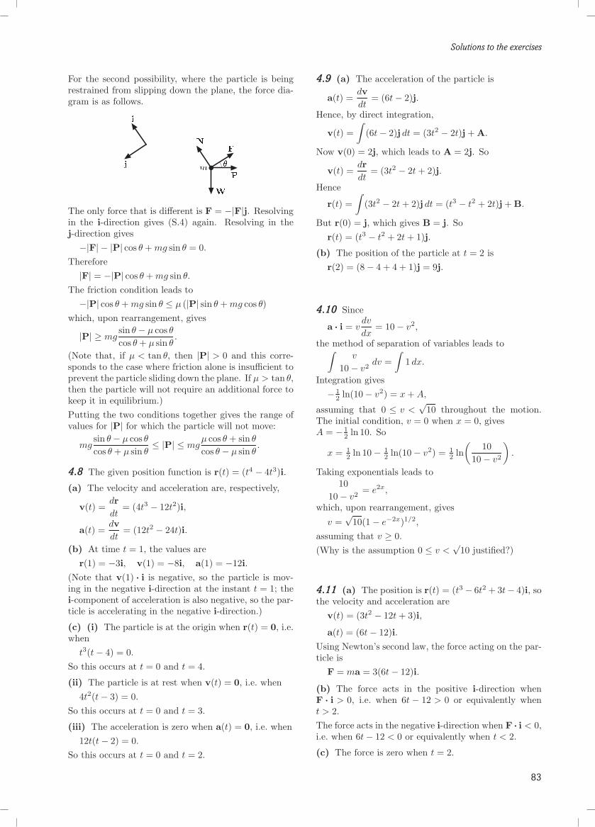
Solutions to the exercises
For the second possibility, where the particle is beingrestrained from slipping down the plane, the force dia-gram is as follows.
The only force that is different is F = −|F|j. Resolvingin the i-direction gives (S.4) again. Resolving in thej-direction gives−|F| − |P| cos θ + mg sin θ = 0.
Therefore|F| = −|P| cos θ + mg sin θ.
The friction condition leads to−|P| cos θ + mg sin θ ≤ µ (|P| sin θ + mg cos θ)
which, upon rearrangement, gives
|P| ≥ mgsin θ− µ cos θ
cos θ + µ sin θ.
(Note that, if µ < tan θ, then |P| > 0 and this corre-sponds to the case where friction alone is insufficient toprevent the particle sliding down the plane. If µ > tan θ,then the particle will not require an additional force tokeep it in equilibrium.)Putting the two conditions together gives the range ofvalues for |P| for which the particle will not move:
mgsin θ− µ cos θ
cos θ + µ sin θ≤ |P| ≤ mg
µ cos θ + sin θ
cos θ− µ sin θ.
4.8 The given position function is r(t) = (t4 − 4t3)i.
(a) The velocity and acceleration are, respectively,
v(t) =drdt
= (4t3 − 12t2)i,
a(t) =dvdt
= (12t2 − 24t)i.
(b) At time t = 1, the values arer(1) = −3i, v(1) = −8i, a(1) = −12i.
(Note that v(1) . i is negative, so the particle is mov-ing in the negative i-direction at the instant t = 1; thei-component of acceleration is also negative, so the par-ticle is accelerating in the negative i-direction.)
(c) (i) The particle is at the origin when r(t) = 0, i.e.when
t3(t− 4) = 0.
So this occurs at t = 0 and t = 4.
(ii) The particle is at rest when v(t) = 0, i.e. when4t2(t− 3) = 0.
So this occurs at t = 0 and t = 3.
(iii) The acceleration is zero when a(t) = 0, i.e. when12t(t− 2) = 0.
So this occurs at t = 0 and t = 2.
4.9 (a) The acceleration of the particle is
a(t) =dvdt
= (6t− 2)j.
Hence, by direct integration,
v(t) =∫
(6t− 2)j dt = (3t2 − 2t)j + A.
Now v(0) = 2j, which leads to A = 2j. So
v(t) =drdt
= (3t2 − 2t + 2)j.
Hence
r(t) =∫
(3t2 − 2t + 2)j dt = (t3 − t2 + 2t)j + B.
But r(0) = j, which gives B = j. Sor(t) = (t3 − t2 + 2t + 1)j.
(b) The position of the particle at t = 2 isr(2) = (8− 4 + 4 + 1)j = 9j.
4.10 Since
a . i = vdv
dx= 10− v2,
the method of separation of variables leads to∫v
10− v2dv =
∫1 dx.
Integration gives− 1
2 ln(10− v2) = x + A,
assuming that 0 ≤ v <√
10 throughout the motion.The initial condition, v = 0 when x = 0, givesA = − 1
2 ln 10. So
x = 12 ln 10− 1
2 ln(10− v2) = 12 ln
(10
10− v2
).
Taking exponentials leads to10
10− v2= e2x,
which, upon rearrangement, gives
v =√
10(1− e−2x)1/2,
assuming that v ≥ 0.(Why is the assumption 0 ≤ v <
√10 justified?)
4.11 (a) The position is r(t) = (t3 − 6t2 + 3t− 4)i, sothe velocity and acceleration are
v(t) = (3t2 − 12t + 3)i,
a(t) = (6t− 12)i.Using Newton’s second law, the force acting on the par-ticle is
F = ma = 3(6t− 12)i.
(b) The force acts in the positive i-direction whenF . i > 0, i.e. when 6t − 12 > 0 or equivalently whent > 2.The force acts in the negative i-direction when F . i < 0,i.e. when 6t− 12 < 0 or equivalently when t < 2.
(c) The force is zero when t = 2.
83

Solutions to the exercises
4.12 (a) The x-axis is chosen to point verticallydownwards with origin at the top of the tower. (Thisensures that x and v are positive throughout the mo-tion.) The only force acting on the marble is assumedto be its weight.
❄i
✉m
❄W
By Newton’s second law, the equation of motion isma = mgi, or equivalently a = g.
(b) Now a = dv/dt = g, hence v = gt + A. The initialcondition, v = 0 when t = 0, leads to A = 0. Hence
v =dx
dt= gt.
Integration givesx = 1
2gt2 + B.
The initial condition, x = 0 when t = 0, gives B = 0.Therefore
x = 12gt2.
The marble reaches the water when x = 10. So10 = 1
2 × 9.81× t2,
and thus
t =
√2× 109.81
/ 1.43 s.
At this time the speed isv = 9.81× 1.43 / 14.0 m s−1.
So the marble hits the water after about 1.43 secondswith a speed of about 14.0m s−1.(Would you expect these values to be increased or de-creased by the effects of air resistance?)
(c) First, determine whether the drag force is linear orquadratic for the marble’s motion through the water.When the marble hits the water,
D|v| = 0.01× 14.0 = 0.14,
so the quadratic model is almost appropriate, and iscertainly more appropriate than the linear model.The force diagram now includes the drag force R.
❄i
✉0.025 kg
❄W
✻R
The forces areW = mgi,
R = −156D|v|v = −1.56v2i,
where v = vi. By Newton’s second law, the equation ofmotion is
ma = mgi− 1.56v2i,
or equivalently,a = g − 1
0.0251.56v2 = g − 62.4v2.
Using a = v dv/dx and separating the variables, thisgives∫
v
9.81− 62.4v2dv = − 1
62.4
∫v
v2 − 0.39652=
∫1 dx.
Integrating, and recognizing from the initial conditionfor entry into the water that v > 0.3965, gives− 1
62.4 × 12 ln(v2 − 0.39652) = x + C.
The initial condition is v = 14.0 when x = 10, so− 1
124.8 ln(142 − 0.39652) = 10 + C.
Therefore C = −10 − 1124.85.277 / −10.04. The speed
with which it hits the bottom of the pool is given by− 1
124.8 ln(v2 − 0.39652) = 11− 10.04,
i.e. byv2 / 0.39652 + e−119.5.
Hence v / 0.3965m s−1 when the marble hits the bot-tom of the pool.
4.13 Choose an x-axis to point vertically upwardswith origin at the point of projection, so x andv are positive throughout the upward motion, andthe initial conditions are r(0) = 0 and v(0) = v0i.During the motion, the forces acting on the parti-cle are its weight, W = −mgi, and air resistance,R = −kv = −kvi (where v = vi), where k is the con-stant of proportionality.
✻i
"m
❄W
❄R
Newton’s second law gives
mdvdt
= −mgi + R = −(mg + kv)i.
Resolving in the i-direction and separating the variablesgives∫
m
mg + kvdv = −
∫1 dt,
som
kln(mg + kv) = −t + A,
since mg + kv > 0 throughout the upward motion. Ini-tially v = v0 when t = 0, which gives
A =m
kln(mg + kv0).
Henceln(mg + kv)− ln(mg + kv0) = −kt/m,
or equivalently,
ln(
mg + kv
mg + kv0
)= −kt
m. (S.5)
Take exponentials to obtainmg + kv
mg + kv0= e−kt/m.
Rearrange this to obtain
v =(mg
k+ v0
)e−kt/m − mg
k.
The particle reaches its maximum height when v = 0.From (S.5) this occurs when
t = −m
kln
(mg
mg + kv0
)=
m
kln
(mg + kv0
mg
).
(Is this value less than or greater than the value thatwould be obtained in the absence of air resistance?)
84

Solutions to the exercises
4.14 (a) There are four forces acting on the parti-cle P : its weight W, the normal reaction N and twospring forces, H1 and H2.
✉ ✲✛✻
❄
H2H1
W
N
✲✻
ij m
The first two forces can be expressed asW = −mgj, N = |N|j.
The lengths of springs AP and PB are x and 1− x, re-spectively. So their extensions are, respectively, x− 0.5and (1 − x) − 0.5 = 0.5 − x. Using Hooke’s law, thespring forces are
H1 = −8(x− 0.5)i,H2 = −4(0.5− x)(−i) = 4(0.5− x)i.
Now m = 3kg, so Newton’s second law gives3xi = H1 + H2 + N + W
= −8(x− 0.5)i + 4(0.5− x)i + N + W.
Hence, on resolving in the i-direction, the equation ofmotion is
3x + 12x = 6.
(b) The particle’s motion is simple harmonic with an-gular frequency ω = 2. So the period of oscillations is
τ =2π
ω= π.
The equilibrium position of the particle, xeq, is givenby the equation of motion with x = 0, i.e. by
12xeq = 6,
so xeq = 12 , which is the same as the particular integral.
(The subsection following this exercise has more exam-ples on oscillating systems.)
4.15 Take the origin at the ceiling with the x-axis ver-tically downwards. There are two forces acting on theparticle: its weight W and the spring force H.
✉✻❄
4 kg
W
H
❄i
When the length of the spring is x, its extension isx− 0.2, so the forces are
H = −36(x− 0.2)i,W = mgi = 4gi.
Newton’s second law gives4xi = 4gi− 36(x− 0.2)i,
sox + 9x = 9.81 + 1.8 = 11.61.
The angular frequency is 3, so the period of oscillationsis 2
3π.The general solution of the equation of motion is
x = 1.29 + B cos(3t + φ),
where B and φ are arbitrary constants. The initial con-ditions are x(0) = 0.5 and x(0) = 0. Substituting theseinto the general solution gives
0.5 = B cos φ + 1.29,
0 = −3B sin φ.
These give B = −0.79 and φ = 0. The particular solu-tion is
x = 1.29− 0.79 cos(3t).The maximum value of x (corresponding to the low-est position of the particle) is when cos(3t) = −1, i.e.xmax = 2.08m.
4.16 (a) There are four forces acting on the parti-cle P : its weight W, the normal reaction N and twospring forces, H1 and H2.
✉ ✲✛✻
❄
H2H1
W
N
✲✻
ij m
The first two forces can be expressed asW = −mgj, N = |N|j.
The lengths of springs AP and PB are x and 3l0−x, re-spectively. So their extensions are, respectively, x− l0and (3l0 − x) − l0 = 2l0 − x. Using Hooke’s law, thespring forces are
H1 = −k(x− l0)i,H2 = −2k(2l0 − x)(−i) = 2k(2l0 − x)i.
Now Newton’s second law givesmxi = H1 + H2 + N + W
= −k(x− l0)i + 2k(2l0 − x)i + N + W.
Hence, on resolving in the i-direction, the equation ofmotion is
mx + 3kx = 5kl0.
(b) The particle’s motion is simple harmonic with an-gular frequency ω given by ω2 = 3k/m. So the periodof oscillations is
τ =2π
ω= 2π
√m
3k.
The equilibrium position of the particle, xeq, is givenby the equation of motion with x = 0, i.e. by
3kxeq = 5kl0,
so xeq = 53 l0.
4.17 (a) The motion is simple harmonic with angularfrequency ω = 2. So
x(t) = B cos(2t) + C sin(2t).Differentiating, the particle’s velocity is
x(t) = −2B sin(2t) + 2C cos(2t).Use the initial conditions, x(0) = 4, x(0) = 6, to obtainB = 4, C = 3. So the position x(t)i is given by
x(t) = 4 cos(2t) + 3 sin(2t),and the velocity x(t)i is given by
x(t) = −8 sin(2t) + 6 cos(2t).
85

Solutions to the exercises
(b) The amplitude of the oscillations is
A =√
B2 + C2 =√
42 + 32 = 5.
(c) At t = π8 , the particle’s position and velocity are
given by
x(π8 ) = 4 cos π
4 + 3 sin π4 = 7√
2= 7
2
√2,
x(π8 ) = −8 sin π
4 + 6 cos π4 = − 2√
2= −
√2.
Hence the position is 72
√2 i and the velocity is −√2 i.
4.18 If x is the height of the ball above the point ofprojection, the gravitational potential energy is mgx.So the law of conservation of mechanical energy gives
12mv2 + mgx = E. (S.6)
Initially v = 20 and x = 0, soE = 1
2m× 202 + mg × 0 = 200m. (S.7)Hence, combine (S.6) and (S.7) to obtain
v2 + 2gx = 400. (S.8)
(a) At maximum height, v = 0. From (S.8) this occurswhen
x = 400/2g / 20.39.
Hence the maximum height of the ball is about 20.4 m.
(b) When x = 15, from (S.8),v2 = 400− 2g × 15 = 105.7.
So the speed of the ball is about 10.3m s−1.
4.19 If x is the length of the spring, its deforma-tion is x− l0. So the potential energy of the spring is12k(x− l0)2, where k is the stiffness of the spring. Usingthe upper end of the spring as datum, the gravitationalpotential energy is −mgx. So the total potential energyis
U = 12k(x− l0)2 −mgx,
and the total mechanical energy isE = 1
2mv2 + 12k(x− l0)2 −mgx. (S.9)
When the particle is released from rest (v = 0), x = l0,so (S.9) becomes E = −mgl0. Hence, by the law ofconservation of mechanical energy,
12mv2 + 1
2k(x− l0)2 −mgx = −mgl0.
When the spring has maximum length, v = 0, so12k(x− l0)2 −mgx + mgl0 = 0. (S.10)
With m = 5, l0 = 0.2 and k = 40, this becomes20x2 − (5g + 8)x + (g + 0.8) = 0,
so
x =5g + 8±√
(5g + 8)2 − 80(g + 0.8)40
=5g + 8± 5g
40=
10g + 840
or840
= 2.6525 or 0.2.
The solution x = 0.2m corresponds to the initial config-uration when the spring has its minimum length. So themaximum length of the spring during the oscillations isabout 2.65m.
(Note, as an alternative, that (S.10) can be factorizedas
(x− l0)(12k(x− l0)−mg) = 0.
Here x − l0 has to be one of the factors, because theparticle is released from rest at x = l0. The remainingfactor gives the required solution as x = l0 + 2mg/k.)
4.20 Using the base of the cliff as the origin, the pathof the stone goes through the point (0, 10) and the point(40, 0). So Equation (4.2) gives
0 = 10 + 40 tan θ− 402 9.812× 202
(1 + tan2 θ),
which reduces to19.62 tan2 θ− 40 tan θ + 9.62 = 0.
This is a quadratic in tan θ and the solution is
tan θ =40±√402 − 4× 19.62× 9.62
2× 19.62/ 1.76 or 0.279.
Therefore the possible launch angles areθ / 1.054 or 0.272 (60.4◦ or 15.6◦).
Using Equation (4.3), the maximum range is given by√(202/9.81)2 + 2× (202/9.81)× 10 / 49.78.
The stone can be thrown to land on the beach almost50m from the base of the cliff.
4.21 There are two parts to the solution. First, useEquation (4.2) to see whether, in the absence of thepartition, there are suitable launch angles. Second, useEquation (4.2) again to see whether either launch angleenables the partition to be cleared.Taking the origin on the floor below the launch point,the launch point is at (0, 1) and the target at (4, 1.5).Substituting these values and u2 = 8g into Equa-tion (4.2) gives
1.5 = 1 + 4 tan θ− 42 g
2× 8g(1 + tan2 θ).
Upon rearrangement, this givestan2 θ− 4 tan θ + 1.5 = 0,
which has roots tan θ = 2±√2.5. So there are two pos-sible launch angles that enable the target to be hit inthe absence of the partition.The top of the partition is at (2, 2.5), so use Equa-tion (4.2) again to see if either of the above launchangles gives y ≥ 2.5 when x = 2. Since
y = 1 + 2 tan θ− 22 g
2× 8g(1 + tan2 θ)
= 1 + 2(2±√
2.5)− 14
(1 + (2±
√2.5)2
)/ 4.71 or 1.54,
only the larger launch angle,
arctan(2 +√
2.5) / 1.298 (74.4 ◦),allows the partition to be cleared.Therefore it is possible for Jane to hit her colleague onthe head with the box of matches, provided that theceiling is more than 4.71m high. (In fact, the highestpoint of the trajectory occurs just after the partition iscrossed, but the height here is also 4.71m to 2 d.p.)
86

Solutions to the exercises
4.22 Taking the take-off point as the origin, use Equa-tion (4.2) to deduce the value of x when y = −2 for thelargest possible launch angle. Since
−2 = 0 + x tan π9 − x2 9.81
2× 92(1 + tan2 π
9 ),
this gives0.068 578x2 − 0.363 970x− 2 = 0.
The positive root of this is approximately 8.67. So, ifthe gap between the buildings is less than 8.67m thenthe policeman can jump from one roof to the other.
4.23 (a) Since m = 3, r = 2 and k = 12, the dampingratio is given by
α =r
2√
mk=
22√
3× 12= 1
6 .
Hence the damping is weak (since α < 1). The naturalangular frequency is
ω =
√k
m=
√123
= 2 s−1,
and the period of the motion is
τ =2π
ω√
1− α2=
6π√35/ 3.186 s.
The equilibrium position is xeq = 6/12 = 0.5.
(b) The displacement of the particle is given byx(t) = xeq + Ae−ρt cos(νt + φ),
where ρ = ωα = 13 , ν = ω
√1− α2 = 1
3
√35, xeq = 0.5.
Differentiating x(t) givesx(t) = −Aρe−ρt cos (νt + φ)−Aνe−ρt sin (νt + φ) .
The initial conditions x(0) = 1 and x(0) = 0 (releasefrom rest) give, respectively,
1 = 0.5 + A cos φ,
0 = −Aρ cos φ−Aν sin φ,
from which tan φ = −ρ/ν with − 12π < φ < 0 (since
cosφ > 0 and tan φ < 0), and A = 0.5/ cosφ. Hence
cosφ =ν√
ν2 + ρ2=
ω√
1− α2√ω2 (1− α2) + ω2α2
=√
1− α2 =√
3536 = 1
6
√35.
Therefore
A = 0.5× 6√35
=3√35/ 0.507
and
φ = − arctan(
1√35
)/ −0.167.
Hence the displacement is
x(t) = 0.5 +3√35
e−t/3 cos(
13
√35t− arctan
(1√35
))/ 0.5 + 0.507e−t/3 cos(1.972t− 0.167).
(c) The graph of this function is shown below.
!5 10
0.4
0.5
0.6
1.0
0 t
x(t)
The particle is within 0.1m of its equilibrium positionwhen it lies within the range 0.4 ≤ x ≤ 0.6. An upperestimate for the latest time T at which the particle en-ters this range and then stays there is given by solvingthe equation
3√35
e−T/3 = 0.1, i.e. T = 3 ln(
30√35
)/ 4.871 s.
A more accurate value for T is found by obtaining thelargest solution of the two equations
3√35
e−T/3 cos(
13
√35T − arctan
(1√35
))= ±0.1.
The graph suggests that this occurs in fact for −0.1 onthe right-hand side. Using a numerical method (e.g. aMathcad solve block), the solution is T / 4.870 s.
4.24 (a) The forces acting on the particle are: itsweight W, the spring force H, the resistance force Rdue to the damper and the normal reaction N. Onepossible force diagram is as follows. (The directionsof H and R could be to the left or right, depend-ing on whether the spring is compressed or extended,and whether the damper is increasing or decreasing inlength. It is usual to consider an extended spring and adamper whose length is increasing. The choice of direc-tions on the force diagram does not affect the results.)
✲i
"✛H✛R
❄
✻N
W
m
Applying Newton’s second law givesmr = H + R + N + W. (S.11)
Now the forces need to be modelled. Start with the forceexerted by the spring. Take the x-axis to be parallel tothe spring and damper, with origin at the fixed end, andi to be a unit vector in the positive x-direction (whichpoints to the right). Then the length of the spring is x,and a unit vector from the centre of the spring to theparticle is i, so Hooke’s law gives
H = −k(x− l0)i, (S.12)where k is the stiffness of the spring and l0 is the naturallength of the spring.
87

Solutions to the exercises
Now consider the model damper, which also has lengthx. The rate of change of length is x, and a unit vectorfrom the centre of the damper to the particle is i. Theforce due to the model damper is
R = −rx i, (S.13)where r is the damping constant. Since the motion ishorizontal, N + W = 0. Substituting (S.12) and (S.13)into (S.11) gives
mr = −k(x− l0)i− rx i.
Resolving in the i-direction and rearranging gives thescalar equation of motion of the particle,
mx + rx + kx = kl0.
(b) Using the same notation and axis as in (a), onepossible force diagram is as follows. (Again, the choiceof directions for H and R in the diagram does not affectthe results.)
✲i
✉✛ ✲H R
❄
✻N
W
m
Applying Newton’s second law givesmr = H + R + W + N. (S.14)
The forces need to be modelled. Start with the modelspring, which is in the same position as in (a), and soexerts the same force, given by
H = −k(x− l0)i. (S.15)Now consider the model damper, which has lengthL − x, where L is the distance between the left-handand right-hand walls. The rate of change of length ofthe model damper is
d
dt(L− x) = −x.
A unit vector from the centre of the model damper tothe particle is −i. The force due to the model damperis
R = −r(−x)(−i) = −rx i, (S.16)where r is the damping constant. Since the motion ishorizontal, W + N = 0. Substituting (S.15) and (S.16)into (S.14) gives
mr = −k(x− l0)i− rx i.
Resolving in the i-direction and rearranging gives thescalar equation of motion of the particle,
mx + rx + kx = kl0.
(This is the same equation as found in (a).)
4.25 (a) The door should return to equilibrium asquickly as possible, but not overshoot. Critical damp-ing is desirable, but difficult to achieve in practice; itwould be better to have damping that is slightly on thestrong side.
(b) If the objective is to minimize the forces experi-enced by the passengers, then slightly weak damping isrequired, to absorb the acceleration caused by the roadsurface. If the objective is to give good road-holding,then the damping should be near critical, to maintainan adequate normal reaction on the road.
(c) In this system the idea is for the baby to be ableto bounce the cradle easily and not to dissipate energy,so very weak damping is required.
4.26 (a) The auxiliary equation is
λ2 + λ + 1 = 0.
Since r2 − 4mk = −3, the damping is weak. The rootsof the auxiliary equation are − 1
2 ± i√
32 . The comple-
mentary function can be written as
xc = Ae−t/2 cos(√
32 t + φ),
where A and φ are constants. As the equation is ho-mogenous, this is also the general solution.
(b) The auxiliary equation is
2λ2 + 3λ + 1 = 0.
Since r2 − 4mk = 1, the damping is strong. The rootsof the auxiliary equation are − 1
2 and −1. The comple-mentary function can be written as
xc = Be−t/2 + Ce−t,
where B and C are constants. A particular integral isxp = 5, so the general solution is
x(t) = Be−t/2 + Ce−t + 5.
(c) The auxiliary equation is
2λ2 + 4λ + 2 = 0.
Since r2 − 4mk = 0, the damping is critical. The auxil-iary equation has one repeated root, −1. The comple-mentary function can be written as
xc = (Bt + C)e−t,
where B and C are constants. A particular integral isxp = 3
2 , so the general solution is
x(t) = (Bt + C)e−t + 32 .
(d) The auxiliary equation is
λ2 + 3λ + 3 = 0.
Since r2 − 4mk = −3, the damping is weak. The rootsof the auxiliary equation are − 3
2 ± i√
32 . The comple-
mentary function can be written as
xc = Ae−3t/2 cos(√
32 t + φ),
where A and φ are constants. A particular integral isxp = 1
6 , so the general solution is
x(t) = Ae−3t/2 cos(√
32 t + φ) + 1
6 .
88

Solutions to the exercises
4.27 To deduce the dimensions of the damping ratio α,first determine the dimensions of each of the other quan-tities in the formula
α =r
2√
mk.
The dimensions of r, the damping constant, can be de-duced from the equation R = −rl s. Now R is a force,so has dimensions MLT−2, and l s is a velocity, so hasdimensions LT−1. Hence
MLT−2 = [r] LT−1,
so [r] = MT−1. The stiffness k has units Nm−1 andhence dimensions MLT−2/L = MT−2. So
[α] =M T−1
1×√M×MT−2=
M T−1
M T−1= 1.
Hence the damping ratio is a dimensionless quantity.
α =1
2√
1× 1= 0.54.28 (a)
α =3
2√
2× 1/ 1.06(b)
α =4
2√
2× 2= 1(c)
α =3
2√
1× 3/ 0.87(d)
4.29 (a) If H denotes the spring force, R the resis-tance force due to the damper, W the particle’s weightand N the normal reaction, one possible force diagramis as follows.
✲i
✉✛ ✛H R ✲P
❄
✻
W
N
m
Applying Newton’s second law to the particle givesmr = H + R + P + N + W. (S.17)
The forces H and R are essentially the same as in So-lution 4.24(a), so
H = −k(x− l0)i,R = −rx i,
P = P cos(Ωt)i.Since the motion is horizontal, N + W = 0, and so(S.17) becomes
mr = −k(x− l0)i− rxi + P cos(Ωt)i.Resolving in the i-direction gives the equation of motion
mx = −k(x− l0)− rx + P cos(Ωt),which is usually written as
mx + rx + kx = kl0 + P cos(Ωt).
(b) Using the same notation as in (a), one possibleforce diagram is as follows.
✲i
✉✛ ✲H R
❄
✻N
W
m
Applying Newton’s second law to the particle givesmr = H + R + N + W. (S.18)
The force exerted by the spring is given by Hooke’s law:H = −k(x− l0)i.
To calculate the force due to the model damper, itslength has to be determined. From the data given in thequestion, the length of the model damper is l = y − x,where y = y0 + a cos(Ωt). So the rate of change oflength of the model damper is
l =d
dt
(y0 + a cos(Ωt)− x
)= −aΩsin(Ωt)− x.
This gives the force exerted by the model damper asR = −r
(−aΩsin(Ωt)− x)(−i)
= −r(aΩ sin(Ωt) + x
)i.
Substituting these forces into (S.18), and using the factthat N + W = 0 (the motion is horizontal), gives
mr = −k(x− l0)i− r(aΩsin(Ωt) + x
)i.
Resolving in the i-direction, and rearranging, gives theequation of motion of the particle as
mx + rx + kx = kl0 − raΩsin(Ωt).
4.30 (a) The magnification factor is
M =kA
P=
k√(k −mΩ2
)2 + r2Ω2
=1√(
1−Ω2)2 + Ω2
=1√
1− Ω2 + Ω4.
(b) The values are best presented as a table.
Ω 0.1 0.2 0.6 0.7 0.8 1.0 1.5M 1.00 1.02 1.14 1.15 1.14 1.00 0.51
(c) A sketch graph of the solution is as follows.
K
'+
,
+)3 ,
(d) From the graph it can be seen that resonance oc-curs approximately when Ω = 0.7.
(e) To find the local minimum of f(x), put the firstderivative equal to zero, and then use the second deriva-tive test. The derivative of f(x) is 2x − 1, and sothe derivative is zero when x = 1
2 . Also, f ′′(x) = 2 sof ′′(1
2 ) = 2, which is positive. So, by the second deriva-tive test, f(x) has a local minimum at x = 1
2 .
89

Solutions to the exercises
(f) Since f(x) has a local minimum at x = 12 it fol-
lows that 1/√
f(x) has a local maximum at x = 12 .
But M = 1/√
f(Ω2), so M has a local maximum when
Ω2 = 12 , i.e. when Ω = 1/
√2. So, to four decimal places,
the resonant angular frequency is 0.7071.
4.31 The arrangement of masses and springs in thisproblem is shown in the following diagram.
(a) The force diagrams are as follows.
✉3
✲i
✛
✻
W1❄
N1
H1 ✉5
✲H2 ✲
H4✛H3
✻
W2❄
N2
The equations of motion for the two particles are3x1i = H1 + H2 + N1 + W1,
5x2i = H3 + H4 + N2 + W2.
The normal reactions and weight forces are the onlyforces in the vertical direction, and since there is no ver-tical motion, N1 + W1 = 0 and N2 +W2 = 0. The fol-lowing table provides expressions for the spring forces.
force H1 H2
length x1 x2 − x1
extension x1 − 1 x2 − x1 − 1
vector s i −i
expression −6(x1 − 1)i 15(x2 − x1 − 1)i
force H3 H4
length x2 − x1 4− x2
extension x2 − x1 − 1 (4− x2)− 2
vector s i −i
expression −15(x2 − x1 − 1)i 10(2− x2)i
The equations of motion become3x1i = − 6(x1 − 1)i + 15(x2 − x1 − 1)i,5x2i = − 15(x2 − x1 − 1)i + 10(2− x2)i.
Resolving these in the i-direction and rearranging givesx1 = − 7x1 + 5x2 − 3,
x2 = 3x1 − 5x2 + 7.
This can be put into matrix form asx = Ax + c,
where
x =
[x1
x2
], A =
[−7 53 −5
]and c =
[−37
].
(b) From Solution 3.20, the general solution to theequations of motion is[
x1
x2
]= C1
[11
]cos
(√2t + φ1
)+ C2
[5
−3
]cos
(√10t + φ2
)+
[12
].
Since there is no initial velocity, φ1 = φ2 = 0. The ini-tial condition for displacements gives[
x1(0)x2(0)
]= C1
[11
]+ C2
[5
−3
]+
[12
]=
[1.51.7
],
i.e.C1 + 5C2 = 0.5, C1 − 3C2 = −0.3.
The solution to these equations is C1 = 0, C2 = 0.1.Hence the required particular solution of the system ofdifferential equations is[
x1
x2
]=
[0.5
−0.3
]cos
(√10t
)+
[12
].
(An alternative approach is to measure displacementsfrom the equilibrium positions, and this is explored inthe subsection following this exercise.)
4.32 (a) The system has one degree of freedom. Thedistance moved along the wire could be chosen as a co-ordinate.
(b) The system has two degrees of freedom. The par-ticle can move anywhere in a plane.
(c) The system has six degrees of freedom. Each par-ticle can move anywhere in a plane.
(d) The system has three degrees of freedom. The an-gles that the rod and the spring make with the verticaland the length of the model spring could be used ascoordinates.
4.33 (a) This is a normal mode with the particles inphase-opposed motion.
(b) This is not a normal mode, since the particles arenot moving sinusoidally.
(c) This is not a normal mode. One way to see thisis to note that the particles do not pass through theirequilibrium positions simultaneously.
(d) This is a normal mode, with motion of the left-most and right-most particles phase-opposed. The mo-tions of all other pairs of particles are neither phase-opposed nor in-phase, since the middle particle is sta-tionary.
90

Solutions to the exercises
4.34 The force diagrams are as follows.
✉m
✲i
✛
✻
W1❄
N1
H1 ✉m
✲H2 ✲
H4✛H3
✻
W2❄
N2
Since x1 and x2 are measured from the equilibrium po-sitions of the particles, this is a situation where themodified form of Newton’s second law given by Equa-tion (4.5) can be applied. This leads to
mr1 = ΔH1 + ΔH2, mr2 = ΔH3 + ΔH4. (S.19)Each of the ΔHi forces can be expressed using the mod-ified form of Hooke’s law, given by Equation (4.6). Theextension of the left-hand spring from its equilibriumlength is x1, and a unit vector from the centre of thespring towards the particle is i, so Equation (4.6) givesΔH1 = −kx1i. Similarly, for ΔH2, the unit vector is−i and the extension from equilibrium length is x2 − x1
(i.e. increasing x2 increases the length of the spring,and increasing x1 decreases the length of the spring).So Equation (4.6) gives
ΔH2 = −k(x2 − x1)(−i) = k(x2 − x1)i.Similarly, for ΔH3 and ΔH4, this leads to
ΔH3 = −ΔH2 = −k(x2 − x1)i,ΔH4 = −k(−x2)(−i) = −kx2i.
Substituting into (S.19) givesmr1 = −kx1i + k(x2 − x1)i,mr2 = −k(x2 − x1)i− kx2i.
Hence, resolving in the i-direction and writing in matrixform, the equation of motion is[
x1
x2
]=
k
m
[−2 11 −2
] [x1
x2
].
4.35 The eigenvalues of the dynamic matrix are k/mtimes those of the matrix[−2 1
1 −2
],
which has the same eigenvectors as the dynamic matrix.Now[−2 1
1 −2
] [11
]=
[−1−1
]= (−1)
[11
]and[−2 1
1 −2
] [1
−1
]=
[−33
]= (−3)
[1
−1
].
So the eigenvalues of[−2 1
1 −2
]are −1 and −3, and
correspondingly, those of the dynamic matrix are −k/mand −3k/m. Hence the normal mode angular frequen-cies are
√k/m and
√3k/m.
4.36 (a) The force diagrams are as follows.
"m ✲H1
❄
✻
W1
N1 "m
✛ ✲H2 H3
❄
✻
W2
N2
✲i
"m✛H4
❄
✻
W3
N3
Apply the modified version of Newton’s second law (4.5)to each particle, to obtainmr1 = ΔH1,
mr2 = ΔH2 + ΔH3,mr3 = ΔH4.
(S.20)
Modelling the forces using the modified version ofHooke’s law (4.6) gives
ΔH1 = −k(x2 − x1)(−i) = k(x2 − x1)i,ΔH2 = −k(x2 − x1)i,ΔH3 = −k(x3 − x2)(−i) = k(x3 − x2)i,ΔH4 = −k(x3 − x2)i.
Substituting these into (S.20), and resolving in thei-direction, gives mx1 = −kx1 + kx2,
mx2 = kx1 − 2kx2 + kx3,mx3 = kx2 − kx3.
(b) In a rigid body motion, all the particles moveat the same velocity, and so an eigenvector must be[1 1 1]T . To verify that this is an eigenvector, mul-tiply by the dynamic matrix, to obtain
k
m
−1 1 01 −2 10 1 −1
111
=
000
= 0
111
.
So [1 1 1]T is an eigenvector with eigenvalue zero.(The corresponding normal mode angular frequency isalso zero.)
(c) A suitable eigenvector is [1 0 − 1]T . To findthe normal mode angular frequency, first find the eigen-value:
k
m
−1 1 01 −2 10 1 −1
10
−1
=k
m
−101
= − k
m
10
−1
.
So [1 0 − 1]T is an eigenvector with eigenvalue−k/m, and the corresponding normal mode angular fre-quency is
√k/m.
(d) A suitable eigenvector is [1 − 2 1]T . To findthe normal mode angular frequency, first find the eigen-value:
k
m
−1 1 01 −2 10 1 −1
1−2
1
=k
m
−36
−3
= −3k
m
1−2
1
.
So [1 − 2 1]T is an eigenvector with eigenvalue−3k/m, and the corresponding normal mode angularfrequency is
√3k/m.
91
