MT5836 Galois Theory

MRQ

May 10, 2019

Contents

Introduction 3Structure of the lecture course . . . . . . . . . . . . . . . . . . . . . . . . . . . . . . . 4Recommended texts . . . . . . . . . . . . . . . . . . . . . . . . . . . . . . . . . . . . . 4

1 Rings, Fields and Polynomials 5Rings . . . . . . . . . . . . . . . . . . . . . . . . . . . . . . . . . . . . . . . . . . . . . 5Fields . . . . . . . . . . . . . . . . . . . . . . . . . . . . . . . . . . . . . . . . . . . . . 7Polynomials . . . . . . . . . . . . . . . . . . . . . . . . . . . . . . . . . . . . . . . . . . 9

2 Field Extensions 17The degree of an extension . . . . . . . . . . . . . . . . . . . . . . . . . . . . . . . . . 17Algebraic elements and algebraic extensions . . . . . . . . . . . . . . . . . . . . . . . . 19Simple extensions . . . . . . . . . . . . . . . . . . . . . . . . . . . . . . . . . . . . . . . 20Minimum polynomials . . . . . . . . . . . . . . . . . . . . . . . . . . . . . . . . . . . . 21

3 Splitting Fields and Normal Extensions 31Splitting fields . . . . . . . . . . . . . . . . . . . . . . . . . . . . . . . . . . . . . . . . 31Existence of splitting fields . . . . . . . . . . . . . . . . . . . . . . . . . . . . . . . . . 33Uniqueness of splitting fields and related isomorphisms . . . . . . . . . . . . . . . . . . 34Normal Extensions . . . . . . . . . . . . . . . . . . . . . . . . . . . . . . . . . . . . . . 37

4 Separability 40Separable polynomials . . . . . . . . . . . . . . . . . . . . . . . . . . . . . . . . . . . . 40Separable extensions and the Theorem of the Primitive Element . . . . . . . . . . . . 44

5 Finite Fields 47Construction of finite fields . . . . . . . . . . . . . . . . . . . . . . . . . . . . . . . . . 47The multiplicative group of a finite field . . . . . . . . . . . . . . . . . . . . . . . . . . 49

6 Galois Groups and the Fundamental Theorem of Galois Theory 52Galois groups . . . . . . . . . . . . . . . . . . . . . . . . . . . . . . . . . . . . . . . . . 52The sets F and G . . . . . . . . . . . . . . . . . . . . . . . . . . . . . . . . . . . . . . 52The Fundamental Theorem of Galois Theory . . . . . . . . . . . . . . . . . . . . . . . 54Examples of Galois groups . . . . . . . . . . . . . . . . . . . . . . . . . . . . . . . . . . 59Galois groups of finite fields . . . . . . . . . . . . . . . . . . . . . . . . . . . . . . . . . 63

7 Solution of Equations by Radicals 65Radical extensions . . . . . . . . . . . . . . . . . . . . . . . . . . . . . . . . . . . . . . 65Soluble groups and other group theory . . . . . . . . . . . . . . . . . . . . . . . . . . . 68Examples of polynomials with abelian Galois groups . . . . . . . . . . . . . . . . . . . 69Galois groups of normal radical extensions . . . . . . . . . . . . . . . . . . . . . . . . . 70A polynomial which is insoluble by radicals . . . . . . . . . . . . . . . . . . . . . . . . 72

1

Galois’s Great Theorem . . . . . . . . . . . . . . . . . . . . . . . . . . . . . . . . . . . 73

2

Introduction

The subject of Galois Theory traces back to Evariste Galois (1811–1832). He was a Frenchmathematician whose work involved understanding the solution of polynomial equations. Thestandard formula

x =−b±

√b2 − 4ac

2a

for the roots of the quadratic equation

ax2 + bx+ c = 0

is well-known. It turns out that analogous formulae exist for the roots of cubic and quarticpolynomial equations. For example, the method to solve the general cubic equation was con-sidered by mathematicians based in Bologna in the early 16th century (e.g., Scipione dal Ferro(1465–1526) and those who followed him).

What Galois did was to show that, in general, a quintic equation could not be solved by asimilar formula. What he did not do was succeed in explaining it to anyone in a comprehensibleway. For example, in 1830 he submitted his work to the Paris Academy of Sciences, but thefinal report states:

We have made every effort to understand Galois’s proof. His reasoning is not suffi-ciently clear, sufficiently developed, for us to judge its correctness, and we can giveno idea of it in this report. The author announces that the proposition which isthe special object of this memoir is part of a general theory susceptible of manyapplications. Perhaps it will transpire that the different parts of a theory are mu-tually clarifying, are easier to grasp together rather than in isolation. We wouldthen suggest that the author should publish the whole of his work in order to form adefinitive opinion. But in the state which the part he has submitted to the Academynow is, we cannot propose to give it approval.

[from Stewart, Galois Theory, Second edition, p.xxi]

Galois’s ideas were eventually understood, via the letter that he wrote to Chevalier on theeve of the duel which killed him. This theory is basically what is presented in this lecture course.As we now understand it, what Galois observed is the following:

• To every polynomial equation, f(x) = 0, we can associate a group, the Galois group,consisting of certain permutations of the roots.

• If the Galois group is soluble, then the polynomial equation can be solved by radicals (thatis, by a formula of the type we are interested in).

• We can construct a polynomial whose Galois group is the symmetric group S5, which isnot soluble since it contains the non-abelian simple group A5, and therefore we cannotsolve the corresponding polynomial equation by radicals.

3

In fact, what we do is more general. We shall actually consider a pair of fields one inside theother (F ⊆ K) and then associate to this a Galois group Gal(K/F ). Our work in this modulewill be to understand the link between the two concepts of the field extension F ⊆ K and itsGalois group. As a consequence of understanding these we can then establish Galois’s aboveobservations by specialising to the case when K is the field obtained by adjoining the roots ofour polynomial f(x) to the field F .

Structure of the lecture course

The following topics will be covered in the lectures:

• Basic facts about fields and polynomial rings: Mostly a review of material fromMT3503, but some new information about irreducible polynomials.

• Field extensions: Terminology and basic properties about the situation of two fieldswith F ⊆ K.

• Splitting fields and normal extensions: Field extensions constructed by adjoiningthe roots of a polynomial, constructed so that the polynomial factorizes into linear factorsover the larger field.

• Basic facts about finite fields: Existence and uniqueness of field of order pn, togetherwith the fact that the multiplicative group of a finite field is cyclic.

• Separable extensions and the Theorem of the Primitive Element: Separability isa technical condition to avoid repeated roots of irreducible polynomials. The Theorem ofthe Primitive Element applies in this circumstance and allows us to assume that our fieldextensions have a specific form and hence to simplify various proofs.

• Galois groups and the Fundamental Theorem of Galois Theory: The definitionof the Galois group as the collection of invertible structure preserving maps of a fieldextension (this will be made more precise later). The Fundamental Theorem of GaloisTheory states that the structure of the Galois group corresponds to the structure of thefield extension.

• Examples and Applications: Including the link between solution of a polynomial equa-tion by radicals and the solubity of the Galois groups.

Recommended texts

• Ian Stewart, Galois Theory, Chapman & Hall; 3rd Edition, 2004 in the library; 4th Edition,2015.

• John M. Howie, Fields and Galois Theory, Springer Undergraduate Mathematics Series,Springer, 2006.

• P. M. Cohn, Algebra, Vol. 2, Wiley, 1977, Chapter 3. [Out of print, but available in thelibrary.]

4

Chapter 1

Rings, Fields and Polynomials

This first chapter contains a review of the background material required to study Galois Theory.The majority comes from the module MT3505 Rings and Fields and consequently many proofsin this chapter are omitted or greatly abbreviated. The last part of this chapter is concernedwith polynomials and polynomial rings. One important concept that we shall use throughoutthe module is what it means for a polynomial to be irreducible. We shall devote some time tomethods for establishing that a polynomial is irreducible.

Rings

We start with properties of rings before specialise to fields and to polynomial rings.

Definition 1.1 A commutative ring with a 1 is a set R endowed with two binary operationsdenoted as addition and multiplication such that the following conditions hold:

(i) R forms an abelian group with respect to addition (with additive identity 0, called zero);

(ii) multiplication is associative: a(bc) = (ab)c for all a, b, c ∈ R;

(iii) multiplication is commutative: ab = ba for all a, b ∈ R;

(iv) the distributive laws hold:

a(b+ c) = ab+ ac

(a+ b)c = ac+ bc

for all a, b, c ∈ R;

(v) there is a multiplicative identity 1 in R satisfying a1 = 1a = a for all a ∈ R.

Comment: There is also a definition of a “ring”, without the assumption of the multiplica-tion being commutative or it having a multiplicative identity 1. One simply drops conditions(iii) and (v) from the definition above. Since we are interested in studying fields in this module,we shall not need to consider non-commutative rings as there will be no examples of such ringsoccurring in these notes. This is why we only give the more restricted definition of a commutativering with a 1 above as this is sufficient for our needs. In addition, note that in a commutativering one needs only assume one of the two distributive laws since the other may be deducedfrom that one via commutativity.

Definition 1.2 Let R be a commutative ring with a 1. An ideal I in R is a non-empty subsetof R that is both an additive subgroup of R and satisfies the property that if a ∈ I and r ∈ R,then ar ∈ I.

5

Thus a subset I of R is an ideal if it satisfies the following four conditions:

(i) I is non-empty (or 0 ∈ I);

(ii) a+ b ∈ I for all a, b ∈ I;

(iii) −a ∈ I for all a ∈ I;

(iv) ar ∈ I for all a ∈ I and r ∈ R.

(In a non-commutative ring, one needs to assume both ar and ra belong to I, but R beingcommutative ensures these products are equal.)

It follows from the definition that an ideal I of R is closed under multiplication: ab ∈ Ifor all a, b ∈ I (since an element b ∈ I is, in particular, an element of the larger set R). Thismeans that an ideal I is, in particular, a subring. Note that, in general, I does not contain themultiplicative identity 1, since if it did r = 1r ∈ I for all r ∈ R. Thus, the only ideal of R thatcontains the multiplicative identity 1 is the ring R itself.

The reason for being interested in ideals is that one can form quotient rings, as we shall nowdescribe. Let R be a commutative ring and let I be an ideal of R. Then I is, in particular, asubgroup of the additive group of R and the latter is an abelian group. We can therefore formthe additive cosets of I; that is, define

I + r = a+ r | a ∈ I

for each r ∈ R. We know from group theory (covered in both MT2505 and MT4003 ) when twosuch cosets are equal,

I + r = I + s if and only if r − s ∈ I,

and that the set of all cosets forms a group via addition of the representatives:

(I + r) + (I + s) = I + (r + s) for r, s ∈ R.

(In arbitrary group, one requires that the subgroup is normal, but this holds because R is anabelian group under addition.) As is observed in MT3505, the assumption that I is an idealthen ensures that there is a well-defined multiplication on the set of cosets, given by

(I + r)(I + s) = I + rs for r, s ∈ R,

with respect to which the set of cosets I + r forms a ring, called the quotient ring and denotedby R/I.

Theorem 1.3 Let R be a commutative ring with a 1 and I be an ideal of R. Then the quotientring R/I is a commutative ring with a 1.

Proof: The fact that R/I is a ring is omitted, since verifying the above operations are well-defined is relatively technical and this was all established in MT3505. That the multiplicationis commutative follows from the fact that the multiplication in R is commutative:

(I + r)(I + s) = I + rs = I + sr = (I + s)(I + r) for all r, s ∈ R.

The multiplication identity is I + 1:

(I + r)(I + 1) = I + r1 = I + r for all r ∈ R.

6

The other standard bit of terminology that we shall require relating to rings is, of course,the definition of a homomorphism. In the following, I shall use the common habit in algebra ofwriting maps on the right, so the image of an element a under a map φ is written aφ (ratherthan φ(a), as would be common in some other branches of mathematics).

Definition 1.4 Let R and S be commutative rings with 1. A homomorphism φ : R → S is amap such that

(i) (a+ b)φ = aφ+ bφ

(ii) (ab)φ = (aφ)(bφ)

for all a, b ∈ R.

Definition 1.5 Let R and S be commutative rings with 1 and φ : R→ S be a homomorphism.

(i) The kernel of φ iskerφ = a ∈ R | aφ = 0 .

(ii) The image of φ isimφ = Rφ = aφ | a ∈ R .

Theorem 1.6 (First Isomorphism Theorem) Let R and S be commutative rings with 1and φ : R → S be a homomorphism. Then the kernel of φ is an ideal of R, the image of φ is asubring of S and

R/kerφ ∼= imφ.

Proof: This is a standard result established in MT3505 (via a proof very similar to that usedfor groups). The isomorphism is the map given by

θ : (kerφ) + a 7→ aφ

for a ∈ R. One must, amongst other things, establish that this is well-defined, in the sense thatthe image of a coset under θ does not depend upon the choice of representative a for the cosetin the quotient ring.

A final set of ring-theoretic definitions are the following, to which we return at the end ofthis chapter.

Definition 1.7 Let R be a commutative ring with a 1.

(i) A zero divisor in R is a non-zero element a such that ab = 0 for some non-zero b ∈ R.

(ii) An integral domain is a commutative ring with a 1 containing no zero divisors.

Fields

Galois Theory can be viewed as the study of fields and their subfields. We shall now presentthe basic facts about such structures.

Definition 1.8 A field F is a commutative ring with a 1 such that 0 6= 1 and every non-zeroelement is a unit, that is, has a multiplicative inverse.

Thus a field F is a commutative ring with a 1 such that (i) there are non-zero elements and(ii) if a ∈ F with a 6= 0, then there exists some b ∈ F with ab = 1. We shall write a−1 or 1/afor the multiplicative inverse of a.

7

Example 1.9 (i) Standard examples of fields familiar from, for example, linear algebra arethe fields Q, R and C of rational numbers, real numbers and complex numbers, respectively.

(ii) If p is a prime number, the set Fp = 0, 1, 2, . . . , p − 1 forms a field under addition andmultiplication modulo p. To see that every non-zero element has a multiplicative inverse,note that if 1 6 x 6 p − 1, then x and p are coprime, so there exists u, v ∈ Z withux + vp = 1 (exploiting the fact that Z is a Euclidean domain). Hence, ux ≡ 1 (mod p)and so, modulo p, u is a multiplicative inverse for x in Fp.

Proposition 1.10 (i) Every field is an integral domain.

(ii) The set of non-zero elements in a field forms an abelian group under multiplication.

We write F ∗ for the multiplicative group of non-zero elements in a field.

Proof: [Omitted in lectures. These facts were observed in MT3505.]Let F be a field.(i) If a, b ∈ F with a 6= 0 and ab = 0, then b = a−1(ab) = 0. Hence if ab = 0, either a = 0 or

b = 0, so F contains no zero divisors.(ii) Write F ∗ = F \ 0. Part (i) tells us that F ∗ is closed under multiplication. The

remaining conditions to be an abelian group under this binary operation follow immediatelyfrom the definition of a field (multiplication is associative in any ring, it is commutative in anycommutative ring, there is a multiplicative identity in any ring with a 1, and in a field everynon-zero element has a multiplicative inverse).

If F is any field, with multiplicative identity denoted by 1, and n is a positive integer, let usdefine

n = 1 + 1 + · · ·+ 1︸ ︷︷ ︸n times

.

By the distributive law,mn = mn

for all positive integers m and n. Since F is, in particular, an integral domain, it follows thatif there exists a positive integer n such that n = 0 then necessarily the smallest such positiveinteger n is a prime number.

Definition 1.11 Let F be a field with multiplicative identity 1.

(i) If it exists, the smallest positive integer p such that p = 0 is called the characteristic of F .

(ii) If no such positive integer exists, we say that F has characteristic zero.

Our observation is therefore that every field F either has characteristic zero or has charac-teristic p for some prime number p. We shall say that K is a subfield of F when K ⊆ F andthat K forms a field itself under the addition and multiplication induced from F ; that is, whenthe following conditions hold:

(i) K is non-empty and contains non-zero elements (or, equivalently when taken with theother two conditions, 0, 1 ∈ K);

(ii) a+ b,−a, ab ∈ K for all a, b ∈ K;

(iii) 1/a ∈ K for all non-zero a ∈ K.

Theorem 1.12 Let F be a field.

8

(i) If F has characteristic zero, then F has a unique subfield isomorphic to the rationals Qand this is contained in every subfield of F .

(ii) If F has characteristic p (prime), then F has a unique subfield isomorphic to the field Fpof integers modulo p and this is contained in every subfield of F .

Definition 1.13 This unique minimal subfield in F is called the prime subfield of F .

Proof: This was proved in MT3505. One proves it as follows:(i) Suppose F has characteristic zero. Extend the notation n to all n ∈ Z by defining

0 = 0 and −n = −n

for all positive integers n. If K is any subfield of F then K contains 0, 1 and all sums involving 1,so n ∈ K for all n ∈ Z. Hence

Q = m/n | m,n ∈ Z, n 6= 0

is a subset of the subfield K.One now verifies, from the field axioms and the assumption that n 6= 0 when n 6= 0, that

the map n 7→ n is a ring homomorphism Z→ F and then extend this to a ring homomorphismQ→ F given by m/n 7→ m/n. We conclude that Q is a subfield of F that is isomorphic to thefield Q of rational numbers and is contained in every subfield K of F .

Finally, uniqueness of Q follows from the minimality condition: if Q1 and Q2 were subfieldscontained in every subfield of F then, in particular, Q1 ⊆ Q2 and Q2 ⊆ Q1, from which wededuce Q1 = Q2.

(ii) Use a similar argument to part (i). If F has characteristic p (prime) and K is any subfieldof F , then K contains all the elements n; that is,

P = 0, 1, 2, 3, . . . , p− 1 ⊆ K.

Now observe that P is closed under addition and multiplication and the map n 7→ n is anisomorphism from the field Fp of p elements to P .

Polynomials

Polynomials arise in a number of places within Galois Theory. The motivation of the subjectarises in the problem of solving polynomial equations. More significantly, algebraic elements,those arising as roots of polynomial equations, will be of great importance in our field extensionsas discussed in Chapter 2.

Definition 1.14 Let F be a field. A polynomial over F in the indeterminate X is an expressionof the form

f(X) = a0 + a1X + a2X2 + · · ·+ anX

n

where n is a non-negative integer and the coefficients a0, a1, . . . , an are elements of F .

We shall often substitute elements of a field for the indeterminate in a polynomial. Thusif α is an element of the field F , or indeed of any field that contains F as a subfield, andf(X) = a0 + a1X + · · ·+ anX

n where the coefficients are also elements in F , we write f(α) forthe expression

f(α) = a0 + a1α+ a2α2 + · · ·+ anα

n.

We shall write F [X] for the set of all polynomials in the indeterminate X with coefficientstaken from the field F . We add two such polynomials by simply adding the coefficients,∑

aiXi +∑

biXi =

∑(ai + bi)X

i,

9

and we multiply two polynomials by exploiting the distributive law:(∑aiX

i)(∑

biXi)

=∑

ciXi

where ck =∑k

i=1 aibk−i. With these definitions, one deduces in a straightforward way thatF [X] forms a commutative ring with a 1, namely the multiplicative identity is the constantpolynomial 1. If f(X) has a non-zero term anX

n of highest degree (that is, all other termsin f(X) has the form aiX

i with i < n) and g(X) has a non-zero term bmXm of highest degree,

then the term of highest degree in f(X)g(X) is anbmXn+m and this is non-zero since F is a

field so anbm 6= 0. Therefore F [X] is actually an integral domain since f(X), g(X) 6= 0 impliesf(X)g(X) 6= 0.

Proposition 1.15 If F is a field, the polynomial ring F [X] is a Euclidean domain.

The Euclidean function associated to F [X] is the degree of a polynomial. Recall that iff(X) = anX

n + an−1Xn−1 + · · ·+ a1X + a0 is a non-zero polynomial with leading term having

non-zero coefficient, that is, an 6= 0, the degree of f(X) is

deg f(X) = n.

The properties of the degree are:

(i) if f(X) and g(X) are non-zero, then deg f(X)g(X) = deg f(X) + deg g(X);

(ii) if f(X) and g(X) are polynomials with f(X) 6= 0, then there exist unique polynomialsq(X) and r(X) satisfying

g(X) = q(X) f(X) + r(X) with either r(X) = 0 or deg r(X) < deg f(X).

These properties were established in MT3505. They are not verified in this module, but will beassumed, and are what is claimed within Proposition 1.15.

As a consequence, all the properties of Euclidean domains established in MT3505 apply toa polynomial ring F [X] over a field F . For example:

Proposition 1.16 If F is a field, the polynomial ring F [X] is a principal ideal domain; thatis, every ideal I in F [X] has the form I =

(f(X)

)= f(X)g(X) | g(X) ∈ F [X] for some

polynomial f(X).

Proof: Let I be an ideal of F [X]. If I = 0, then I = (0). Suppose that I 6= 0. Letf(X) be a polynomial in I such that deg f(X) is as small as possible among the degrees ofnon-zero polynomials in I. Certainly

(f(X)

)⊆ I, since I is closed under multiplication by any

polynomial.Now if g(X) ∈ I, divide f(X) to obtain a quotient and remainder:

g(X) = q(X) f(X) + r(X)

where either r(X) = 0 or deg r(X) < deg f(X). Then r(X) = g(X)− q(X) f(X) belongs to I,since I is an ideal. By the assumption about f(X) having smallest degree amongst non-zeropolynomials in I, we conclude r(X) = 0. Hence g(X) is indeed a multiple of f(X). Thisestablishes I =

(f(X)

), as claimed.

Another fact that holds as a consequence of Proposition 1.15 concerns the greatest commondivisor of a pair (or more) of polynomials.

10

Definition 1.17 Suppose f(X) and g(X) are polynomials over the field F . A greatest commondivisor of f(X) and g(X) is a polynomial h(X) of greatest degree such that h(X) divides bothf(X) and g(X).

To say that h(X) divides f(X) means that f(X) is a multiple of h(X); that is, f(X) =h(X) q(X) for some q(X) ∈ F [X]. In a general Euclidean domain, the greatest common divisoris defined uniquely up to multiplication by a unit. In the polynomial ring F [X], the units areconstant polynomials (that is, elements of the base field F viewed as elements of F [X]). Thisfollows from the first property of degrees listed: deg f(X)g(X) = deg f(X) + deg g(X), so theonly way that f(X)g(X) = 1 can hold is if deg f(X) = 0. As a consequence, the greatestcommon divisor of a pair of polynomials is defined uniquely up to multiplication by a scalarfrom the field F .

We shall need at times the following fact about the form of the greatest common divisor ina Euclidean domain. This result is often accompanied with a practical algorithm for computingthe greatest common divisor, but that will not be as important in this module. The proof ofthe result can be found in MT3505.

Theorem 1.18 Let F be a field and f(X) and g(X) be two non-zero polynomials over F . Thenthere exist u(X), v(X) ∈ F [X] such that the greatest common divisor of f(X) and g(X) is givenby

h(X) = u(X) f(X) + v(X) g(X).

Another standard fact about a Euclidean domain is that it is necessarily a unique factoriza-tion domain. Consequently, every polynomial over F can be factorized as a product of irreduciblepolynomials and these irreducible factors are determined uniquely up to multiplication by scalars(as the units are the constant polynomials) and reordering of the factors (of course, since mul-tiplication is commutative). In view of this, we record the definition of what it means for apolynomial to be irreducible, since that will be a particularly significant concept in terms ofwhat follows.

Definition 1.19 Let f(X) be a polynomial over a field F of degree at least 1. We saythat f(X) is irreducible over F if it cannot be factorized as f(X) = g1(X) g2(X) whereg1(X) and g2(X) are polynomials in F [X] of degree smaller than f(X).

Thus, a polynomial f(X) is irreducible if the only polynomials of degree smaller than f(X)that divide it are the constant polynomials (i.e., the units). The term reducible is used for apolynomial that is not irreducible; that is, that can be factorized as a product of two polynomialsof smaller degree. It will be important to be able to show that certain polynomials are irreducible.In general, this is rather difficult to achieve and one generally needs to rely upon ad hoc methods,particularly over fields of characteristic p > 0.

We first make the observation that the concept of irreducibility depends heavily upon thefield over which we are working. After that we shall consider various examples of methods forshowing polynomials are irreducible.

Example 1.20 Consider the polynomial f(X) = X2 +1. If we view f(X) as a polynomial overthe real numbers R, then it is irreducible: if it were to factorize then it would be a product oftwo linear factors. However, the roots of this polynomial do not exist in the real numbers, sof(X) has no roots in R and hence is irreducible over R. However, when viewed as a polynomialover C, it is reducible:

X2 + 1 = (X − i)(X + i)

Similary g(X) = X2−2 is irreducible over Q (since it has no roots in Q, so can have no linearfactors), but is reducible over R (since it factorizes over this field as X2−2 = (X−

√2)(X+

√2).

11

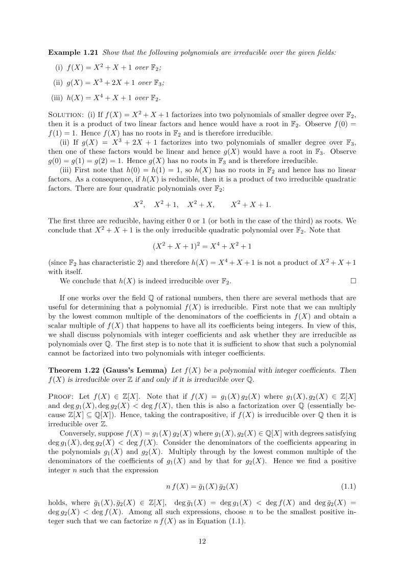
Example 1.21 Show that the following polynomials are irreducible over the given fields:

(i) f(X) = X2 +X + 1 over F2;

(ii) g(X) = X3 + 2X + 1 over F3;

(iii) h(X) = X4 +X + 1 over F2.

Solution: (i) If f(X) = X2 +X + 1 factorizes into two polynomials of smaller degree over F2,then it is a product of two linear factors and hence would have a root in F2. Observe f(0) =f(1) = 1. Hence f(X) has no roots in F2 and is therefore irreducible.

(ii) If g(X) = X3 + 2X + 1 factorizes into two polynomials of smaller degree over F3,then one of these factors would be linear and hence g(X) would have a root in F3. Observeg(0) = g(1) = g(2) = 1. Hence g(X) has no roots in F3 and is therefore irreducible.

(iii) First note that h(0) = h(1) = 1, so h(X) has no roots in F2 and hence has no linearfactors. As a consequence, if h(X) is reducible, then it is a product of two irreducible quadraticfactors. There are four quadratic polynomials over F2:

X2, X2 + 1, X2 +X, X2 +X + 1.

The first three are reducible, having either 0 or 1 (or both in the case of the third) as roots. Weconclude that X2 +X + 1 is the only irreducible quadratic polynomial over F2. Note that

(X2 +X + 1)2 = X4 +X2 + 1

(since F2 has characteristic 2) and therefore h(X) = X4 +X + 1 is not a product of X2 +X + 1with itself.

We conclude that h(X) is indeed irreducible over F2.

If one works over the field Q of rational numbers, then there are several methods that areuseful for determining that a polynomial f(X) is irreducible. First note that we can multiplyby the lowest common multiple of the denominators of the coefficients in f(X) and obtain ascalar multiple of f(X) that happens to have all its coefficients being integers. In view of this,we shall discuss polynomials with integer coefficients and ask whether they are irreducible aspolynomials over Q. The first step is to note that it is sufficient to show that such a polynomialcannot be factorized into two polynomials with integer coefficients.

Theorem 1.22 (Gauss’s Lemma) Let f(X) be a polynomial with integer coefficients. Thenf(X) is irreducible over Z if and only if it is irreducible over Q.

Proof: Let f(X) ∈ Z[X]. Note that if f(X) = g1(X) g2(X) where g1(X), g2(X) ∈ Z[X]and deg g1(X),deg g2(X) < deg f(X), then this is also a factorization over Q (essentially be-cause Z[X] ⊆ Q[X]). Hence, taking the contrapositive, if f(X) is irreducible over Q then it isirreducible over Z.

Conversely, suppose f(X) = g1(X) g2(X) where g1(X), g2(X) ∈ Q[X] with degrees satisfyingdeg g1(X),deg g2(X) < deg f(X). Consider the denominators of the coefficients appearing inthe polynomials g1(X) and g2(X). Multiply through by the lowest common multiple of thedenominators of the coefficients of g1(X) and by that for g2(X). Hence we find a positiveinteger n such that the expression

n f(X) = g1(X) g2(X) (1.1)

holds, where g1(X), g2(X) ∈ Z[X], deg g1(X) = deg g1(X) < deg f(X) and deg g2(X) =deg g2(X) < deg f(X). Among all such expressions, choose n to be the smallest positive in-teger such that we can factorize n f(X) as in Equation (1.1).

12

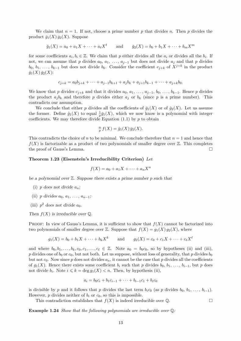
We claim that n = 1. If not, choose a prime number p that divides n. Then p divides theproduct g1(X) g2(X). Suppose

g1(X) = a0 + a1X + · · ·+ a`X` and g2(X) = b0 + b1X + · · ·+ bmX

m

for some coefficients ai, bi ∈ Z. We claim that p either divides all the ai or divides all the bi. Ifnot, we can assume that p divides a0, a1, . . . , aj−1 but does not divide aj and that p dividesb0, b1, . . . , bk−1 but does not divide bk. Consider the coefficient cj+k of Xj+k in the productg1(X) g2(X):

cj+k = a0bj+k + · · ·+ aj−1bk+1 + ajbk + aj+1bk−1 + · · ·+ aj+kb0.

We know that p divides cj+k and that it divides a0, a1, . . . , aj−1, b0, . . . , bk−1. Hence p dividesthe product ajbk and therefore p divides either aj or bk (since p is a prime number). Thiscontradicts our assumption.

We conclude that either p divides all the coefficients of g1(X) or of g2(X). Let us assumethe former. Define g1(X) to equal 1

p g1(X), which we now know is a polynomial with integercoefficients. We may therefore divide Equation (1.1) by p to obtain

np f(X) = g1(X) g2(X).

This contradicts the choice of n to be minimal. We conclude therefore that n = 1 and hence thatf(X) is factorizable as a product of two polynomials of smaller degree over Z. This completesthe proof of Gauss’s Lemma.

Theorem 1.23 (Eisenstein’s Irreducibility Criterion) Let

f(X) = a0 + a1X + · · ·+ anXn

be a polynomial over Z. Suppose there exists a prime number p such that

(i) p does not divide an;

(ii) p divides a0, a1, . . . , an−1;

(iii) p2 does not divide a0.

Then f(X) is irreducible over Q.

Proof: In view of Gauss’s Lemma, it is sufficient to show that f(X) cannot be factorized intotwo polynomials of smaller degree over Z. Suppose that f(X) = g1(X) g2(X), where

g1(X) = b0 + b1X + · · ·+ bkXk and g2(X) = c0 + c1X + · · ·+ c`X

`

and where b0, b1, . . . , bk, c0, c1, . . . , c` ∈ Z. Note a0 = b0c0, so by hypotheses (ii) and (iii),p divides one of b0 or c0, but not both. Let us suppose, without loss of generality, that p divides b0but not c0. Now since p does not divides an, it cannot be the case that p divides all the coefficientsof g1(X). Hence there exists some coefficient bi such that p divides b0, b1, . . . , bi−1, but p doesnot divide bi. Note i 6 k = deg g1(X) < n. Then, by hypothesis (ii),

ai = b0ci + b1ci−1 + · · ·+ bi−1c1 + bic0

is divisible by p and it follows that p divides the last term bic0 (as p divides b0, b1, . . . , bi−1).However, p divides neither of bi or c0, so this is impossible.

This contradiction establishes that f(X) is indeed irreducible over Q.

Example 1.24 Show that the following polynomials are irreducible over Q:

13

(i) Xn − p, for any prime number p;

(ii) 29X

5 + 53X

4 +X3 + 13 ;

(iii) Xp−1 +Xp−2 + · · ·+X2 +X + 1, for any prime number p.

Solution: (i) Xn − p is irreducible by Eisenstein’s Criterion: it is of the form to apply Theo-rem 1.23.

(ii) If f(X) = 29X

5 + 53X

4 +X3 + 13 , then

9f(X) = 2X5 + 15X4 + 9X3 + 3.

Thus 9f(X) is irreducible over Q by Eisenstein’s Criterion (using the prime p = 3), so cannotbe factorized as a product of polynomials of smaller degree over Q. The same therefore appliesto f(X). (Note that 9 is a unit in Q[X].)

(iii) Write Φ(X) = Xp−1 +Xp−2 + · · ·+X2 +X + 1. Suppose Φ(X) can be factorized as aproduct of polynomials of smaller degree over Q; say, Φ(X) = g(X)h(X). Note

(X − 1) · Φ(X) = (X − 1)(Xp−1 +Xp−2 + · · ·+X + 1) = Xp − 1.

Substitute Y = X − 1:

Y · Φ(Y + 1) = (Y + 1)p − 1 =

p∑i=1

(p

i

)Y i.

Hence

Φ(Y + 1) =

p∑i=1

(p

i

)Y i−1

= Y p−1 +

(p

p− 1

)Y p−2 +

(p

p− 2

)Y p−3 + · · ·+

(p

2

)Y +

(p

1

).

The constant coefficient in Φ(Y + 1) is(p1

)= p, which is divisible by p but not p2. Note that,

for i = 1, 2, . . . , p− 1,(p

i

)=

p!

i! (p− i)!=p(p− 1)(p− 2) . . . (p− i+ 1)

i!

and we know this is an integer. Note that the prime p is bigger than all the factors in i! (byassumption on i), so

the binomial coefficient

(p

i

)is divisible by the prime p for i = 1, 2, . . . , p− 1. (1.2)

Hence we may apply Eisenstein’s Criterion to Φ(Y +1) to conclude that Φ(Y +1) is irreducible asa polynomial in Y . Our original assumption, however, implies that Φ(Y +1) = g(Y +1)h(Y +1),which is a contradiction.

Hence Φ(X) is indeed irreducible over Q.

There is one final method that we mention for showing a polynomial (with integer coefficients)is irreducible is to reduce the coefficients modulo some prime p. The choice of prime p is usuallydelicate: when the type of argument presented here applies, it typically does so for some choicesof prime but not others.

Example 1.25 Show that the polynomial f(X) = X4 + 8X3 + 9X2 + 6X + 5 is irreducibleover Q.

14

Solution: Suppose that f(X) is reducible over Q. Then f(X) is reducible over Z, by Gauss’sLemma, so factorizes as a product of polynomials with integer coefficients of smaller degree.

We shall reduce all the coefficients modulo 3. To be more precise, there is a ring homomor-phism φ : Z→ F3 that arises by reducing an integer modulo 3. The kernel of φ is the ideal (3) ofall multiples of 3. We induce a map φ : Z[X]→ F3[X] by applying φ to the coefficients in a poly-nomial; that is, reducing the coefficients modulo 3. Since the coefficients of sums of polynomialsand products of polynomials are determined by operations in the base ring/field, it follows, fromthe fact that φ is a homomorphism, the induced map φ is a ring homomorphism Z[X]→ F3[X].Applying φ to the factorization of f(X) as a product of two polynomials from Z[X], we concludethat

f(X) = f(X)φ = X4 + 2X3 + 2

factorizes; that is, f(X) is reducible over F3. We shall show this is impossible.First note

f(0) = 2, f(1) = 2, f(2) = 24 + 24 + 2 = 1,

so that f(X) does not have any roots in F3 and hence has no linear factors. Therefore f(X) mustbe a product of quadratic factors:

X4 + 2X3 + 2 = (X2 + aX + b)(X2 + cX + d)

for some coefficients a, b, c, d ∈ F3. Equating coefficients:

a+ c = 2, ac+ b+ d = 0,

ad+ bc = 0, bd = 2

The constant coefficient tells us that either b = 1 and d = 2, or b = 2 and d = 1. Thus b+d = 0.The degree 2 coefficient then tells us ac = 0, so either a = 0 or c = 0. The degree 1 coefficientthen tells us that the other of a or c is also zero. Then a + c = 0, so the degree 3 coefficientequation fails.

In conclusion, f(X) is irreducible over F3 and we then deduce the original assumptionabout f(X) was incorrect. Hence f(X) is indeed irreducible over Q.

The final fact about integral domains, that we shall apply to the polynomial ring F [X], isthat every integral domain has a field of fractions. To be precise, if R is an integral domain,the field of fractions of R is the set of all expressions of the form r/s where (i) r, s ∈ R withs 6= 0, and (ii) we define r1/s1 = r2/s2 if and only if r1s2 = r2s1. (The latter condition definesan equivalence relation on ordered pairs (r, s) with s 6= 0 and we write r/s for the equivalencecontaining the ordered pair (r, s) under this equivalence relation.) Mirroring the definition ofaddition and multiplication on the rational numbers, we define

r1

s1+r2

s2=r1s2 + r2s1

s1s2and

r1

s1· r2

s2=r1r2

s1s2

for such fractions r1/s1 and r2/s2. One verifies that the set of all such fractions forms a commu-tative ring under this operation and that every non-zero fraction r/s (that is, when both r and sare non-zero) has a multiplicative inverse, namely s/r, because

r

s· sr

=rs

rs=

1

1

from the definition of when two fractions are equal. The latter is the multiplicative identity inthe field of fractions. Notice finally that R embeds in the field of fractions via the map r 7→ r/1;that is, the set r/1 | r ∈ R is a subring isomorphic to the original integral domain R.

Let us apply this construction in the case when R = F [X], the integral domain of polynomialswith coefficients from the field F . We consequently construct the following object:

15

Definition 1.26 Let F be a field. The field of rational functions with coefficients in F isdenoted by F (X) and is the field of fractions of the polynomial ring F [X].

The elements of F (X) are expressions of the form

f(X)

g(X)

where f(X) and g(X) are polynomials with coefficients from F . Equality of two such expressionsis given by

f1(X)

g1(X)=f2(X)

g2(X)if and only if f1(X) g2(X) = f2(X) g1(X).

If one exploits the fact that F [X] is a unique factorization domain, one can deduce from this thatf2(X) and g2(X) are obtained from f1(X) and g1(X) via cancelling and then multiplying by somecommon factors. Addition in F (X) is achieved by placing a pair of fractions over a commondenominator. The polynomial f(X) is identified with its image f(X)/1 in the field F (X).Thus, we view the polynomial ring F [X] as a subring of the field F (X) of rational functions. Inparticular, since the constant polynomials form a copy of F , we observe:

Proposition 1.27 The field F occurs as a subfield of the field F (X) of rational functions withcoefficients in F .

16

Chapter 2

Field Extensions

This chapter introduces the primary terminology that will be used throughout the module.Galois Theory is essentially the study of fields satisfying F ⊆ K; that is, what we call a fieldextension. We shall present here the basic technology required to work with such extensions.

Definition 2.1 Let F and K be fields such that F is a subfield of K. We then say that K isan extension of F . We also call F the base field of the extension.

In particular, note that every field is an extension of its prime subfield. The point of thisdefinition, though, is a change of perspective. We are not viewing a field extension F ⊆ Kas being the situation where we start with a field K and then pass to a subfield F . Instead,the philosophy here will be much more starting with a base field F and then creating a biggerfield K containing F that is the extension. We shall flesh out this viewpoint initially over thecourse of the chapter and subsequently over the whole module.

The degree of an extension

The first observation to make in this setting is that if the field K is an extension of the field F ,then K, in particular, satisfies the following conditions:

• K forms an abelian group under addition;

• we can multiply elements of K by elements of F ;

• a(x+ y) = ax+ ay for all a ∈ F and x, y ∈ K;

• (a+ b)x = ax+ bx for all a, b ∈ F and x ∈ K;

• (ab)x = a(bx) for all a, b ∈ F and x ∈ K;

• 1x = x for all x ∈ K.

Thus, we can view K as a vector space over the field F .

Definition 2.2 Let the field K be an extension of the field F .

(i) The degree of K over F is the dimension of K when viewed as a vector space over F . Wedenote this by |K : F |. Thus

|K : F | = dimF K.

(ii) If the degree |K : F | is finite, we say that K is a finite extension of F .

17

Warning: Note that saying K is a finite extension of F does not mean that K is a finite field.There are many situations where both fields have infinitely many elements in them. It refersprecisely to the dimension of the bigger field over the smaller field.

Example 2.3 (i) The field C of complex numbers is an extension of the field R of realnumbers. Every complex number can be written as x + iy where x, y ∈ R and it followsthat 1, i is a basis for the set of complex numbers when viewed as a real vector space.Hence

|C : R| = 2;

that is, this is a degree 2 extension.

(ii) The field R of real numbers is an extension of the field Q of rational numbers. Any finitedimensional vector space V over Q is countable, since if v1, v2, . . . , vn is a basis for Vover Q, then there are countably many elements of the form

α1v1 + α2v2 + · · ·+ αnvn

with α1, α2, . . . , αn ∈ Q. Since R is uncountable, we conclude that R is not a finiteextension of Q; it has infinite degree over Q.

Theorem 2.4 (Tower Law) Let F ⊆ K ⊆ L be field extensions. Then L is a finite extensionof F if and only if L is a finite extension of K and K is a finite extension of F . In such a case,

|L : F | = |L : K| · |K : F |.

Proof: First suppose that L is a finite extension of F . This means that, when viewed as avector space over F , L is finite-dimensional. Now K ⊆ L and K is closed under addition andby multiplication by elements of F (since it is a field). Hence K is a subspace of L, when viewedas a vector space over F , and so is also finite-dimensional over F .

Let B = x1, x2, . . . , xk be a basis for L over F . Then every element of L can be writtenin the form

a1x1 + a2x2 + · · ·+ akxk (2.1)

where a1, a2, . . . , ak ∈ F . Therefore, every element of L can also be written in the form (2.1)where we choose the coefficients ai from the field K. (We certainly get all the linear combinationsbuilt using scalars from F and cannot produce elements outside L since K is a subfield of L.)Hence B spans L when viewed as vector space over K and so we conclude |L : K| <∞.

Conversely, suppose that both |L : K| and |K : F | are finite. Let v1, v2, . . . , vm be a basisfor L over K and let w1, w2, . . . , wn be a basis for K over F . We claim that the set of productsB = viwj | 1 6 i 6 m, 1 6 j 6 n is a basis for L over F .

First note that if x ∈ L, then we can express x in terms of the basis for L over K, to deducethat there exist a1, a2, . . . , am ∈ K such that

x =

m∑i=1

aivi.

Now, for each i, express ai in terms of the basis for K over F to find bi1, bi2, . . . , bin ∈ F suchthat

ai =n∑j=1

bijwj .

18

Substitute this into the previous sum to conclude

x =

m∑i=1

n∑j=1

bijviwj

and we conclude that B does indeed span L as a vector space over F .Now suppose that for some coefficients cij ∈ F such that

m∑i=1

n∑j=1

cijviwj = 0.

First express this asm∑i=1

( n∑j=1

cijwj

)vi = 0

and use the fact that v1, v2, . . . , vm is a basis for L over K to conclude that, for i = 1, 2,. . . , m, the elements

n∑j=1

cijwj

in K are all equal to 0. Now use the fact that w1, w2, . . . , wn is a basis for K over F to deduce

cij = 0 for all i and j.

We therefore conclude that B is indeed a basis for L over F . In conclusion, L is a finite extensionof F and

|L : F | = |B| = mn = |L : K| · |K : F |.

Comment: We shall need the observation made in the course of the proof later, so we makethis explicit: In the setting of the theorem, if v1, v2, . . . , vm is a basis for L over K andw1, w2, . . . , wn is a basis for K over F , then viwj | 1 6 i 6 m, 1 6 j 6 n is a basis for Lover F .

Algebraic elements and algebraic extensions

The central results presented in this module will concern finite extensions and accordingly weseek to establish detailed information about such extensions. The first step is understand theconcept of algebraic elements and their link to polynomial equations. Later in this chapter weshall show that we can characterize finite extensions in terms of algebraic elements.

Definition 2.5 Let the field K be an extension of the field F .

(i) An element α ∈ K is said to be algebraic over F if there exists a non-zero polyno-mial f(X) ∈ F [X] such that f(α) = 0. When this holds, we shall say that α satisfiesthe polynomial equation f(X) = 0.

(ii) We say that K is an algebraic extension of F if every element of K is algebraic over F .

Thus to say that an element α ∈ K is algebraic over the subfield F is to say that there arecoefficients b0, b1, . . . , bn in F such that

b0 + b1α+ b2α2 + · · ·+ bnα

n = 0.

19

The first observation to make is that every element α of the base field F is algebraic over Fsince it is a root of the linear (i.e., degree 1) polynomial X−α. The interesting question is thenwhich other elements of K also happen to be algebraic over F . Indeed in the context of finiteextensions, our first, and important, observation is the following.

Lemma 2.6 Every finite extension is an algebraic extension.

Proof: Let K be an extension of F of degree n. Let α ∈ K. Then the n+ 1 elements

1, α, α2, . . . , αn

are linearly dependent over F , so there exist coefficients b0, b1, . . . , bn in F , not all of which arezero, such that

b0 + b1α+ b2α2 + · · ·+ bnα

n = 0.

Hence α satisfies a non-zero polynomial over F (namely f(X) = b0 + b1X + · · · + bnXn), so is

algebraic over F .

Simple extensions

To continue our investigation of finite extensions, we introduce the following notation to describehow a field extension is formed. It enables us to view an extension as formed from a base fieldby introducing further elements.

Definition 2.7 Let the field K be an extension of the field F and α1, α2, . . . , αn be elementsof K. We write

F (α1, α2, . . . , αn)

for the smallest subfield of K that contains both F and the elements α1, α2, . . . , αn.

It is straightforward to verify that the intersection of a collection of subfields of K is again asubfield (see Problem Sheet I, Question 2; one just needs to verify the conditions listed in Chap-ter 1 on page 8). Consequently, the “smallest subfield” containing F and the elements α1, α2,. . . , αn makes sense: it is the intersection of all the subfields of K that contain this collectionof elements. It is possible to describe more explicitly the elements of the field F (α1, α2, . . . , αn)in general, but we shall mainly concentrate on a special case.

Definition 2.8 We say that the field K is a simple extension of the field F if K = F (α) forsome α ∈ K. We then also say that K is obtained by adjoining the element α to F .

Simple extensions will be of great importance. In the case that α is algebraic over F , weshall have a precise description of elements in the simple extension F (α) and good knowledge ofthe degree |F (α) : F | (see Theorem 2.14 below). For a general extension K = F (α1, α2, . . . , αn)obtained by adjoining a finite collection of elements to a base field F , we can view this as achain of simple extensions,

F ⊆ F (α1) ⊆ F (α1, α2) ⊆ · · · ⊆ F (α1, α2, . . . , αn)

since at each stage F (α1, . . . , αi) is the simple extension obtained by adjoining the element αito the previous subfield F (α1, . . . , αi−1).

Example 2.9 Let F be a field and X be an indeterminate. The field F (X) of rational functionsis a simple extension of F .

Indeed, in Proposition 1.27 we observed that F occurs as a subfield of F (X), so F (X) isindeed an extension of F . The elements of F (X) has the form f(X)/g(X) where f(X) and g(X)

20

are polynomials with coefficients from F . Now if L is any subfield of F (X) that contains thesubfield F and the element X, then it first contains all polynomials in X, since L is closedunder multiplication and addition. It is also closed under quotients and hence contains allquotients f(X)/g(X) where f(X) and g(X) are polynomials. Therefore L = F (X). We concludethat F (X) indeed equals its smallest subfield containing F and the indeterminate X.

Thus the field F (X) of rational functions is the simple extension of F obtained by adjoiningthe indeterminate X. In particular, the notation F (X) as introduced in Definition 1.26 isconsistent with that in Definition 2.8. Moreover, X is not an algebraic element over F : if b0, b1,. . . , bn are elements of F , not all of which are zero, then

b0 + b1X + b2X2 + · · ·+ bnX

n

is some non-zero polynomial f(X) and so non-zero in the field F (X) of rational functions. Theterm transcendental is used for an element that is not algebraic over the base field. Thus theindeterminate X as used in F (X) is transcendental over the base field F . In fact, it turns out —though not so significant for this module — that if α is any transcendental element over the basefield F , then the simple extension F (α) is isomorphic to the field F (X) of rational functions.

Minimum polynomials

We shall be most interested in simple extensions F (α) where α is algebraic over the base field F .The most important definition we need in this context is the following:

Definition 2.10 Let F be a field and α be an element in some field extension of F such thatα is algebraic over F . The minimum polynomial of α over F is the monic polynomial f(X) ofleast degree in F [X] such that f(α) = 0.

Recall that a polynomial is monic if its leading term has coefficient 1. (The minimumpolynomial is also sometimes called the “minimal polynomial” in some sources.)

One can apply very similar arguments to those used in linear algebra to establish quitedirectly that the minimum polynomial of an algebraic element exists and is unique. We shall,however, use a more ring-theoretic flavour of argument since that will also set up the technologywe shall use to understand the structure of a simple extension.

Let α be an element in some extension of the field F that is algebraic over F . Define a mapφ : F [X]→ F (α) by evaluating a polynomial at α:

φ : g(X) 7→ g(α).

We shall first observe that φ is a ring homomorphism. This is actually quite straightforward anddepends upon only the ring axioms holding in the field F (α), but we shall check it explicitly.

Consider two polynomial g(X), h(X) ∈ F [X], say

g(X) =∑

aiXi and h(X) =

∑biX

i

(where we understand that these are finite sums: all but finitely many ai and bi are zero). Then

g(X)φ+ h(X)φ = g(α) + h(α)

=∑

aiαi +∑

biαi

=∑

(ai + bi)αi

= (g + h)(α)

=(g(X) + h(X)

)φ

21

and

g(X)φ · h(X)φ = g(α)h(α)

=(∑

aiαi)(∑

biαi)

=∑

ciαi,

where ci =∑i

j=0 ajbi−j , by the distributive laws. Note g(X)h(X) =∑ciX

i, by definition, so

g(X)φ · h(X)φ =(g(X)h(X)

)φ.

Hence φ is a ring homomorphism. The First Isomorphism Theorem (Theorem 1.6) tells us that

F [X]

kerφ∼= imφ

and imφ is some subring of F (α). (The latter field contains F , α and is closed, in particular,under products and sums, so necessarily contains all g(α).) The assumption that α is algebraicensures there exist some non-zero polynomials g(X) satisfying g(α) = 0; that is, kerφ 6= 0. Thefact that F [X] is a principal ideal domain tells us that

kerφ =(f(X)

)for some polynomial f(X). Moreover, the proof of Proposition 1.16 tells us that deg f(X) isminimal amongst all non-zero polynomials g(X) in kerφ; that is, amongst all non-zero polyno-mials g(X) satisfying g(α) = 0. Finally, note that the scalars are units in F [X], so we may divideby the coefficient of the leading terms of f(X), without changing the ideal generated by f(X),and hence assume f(X) is monic; that is, f(X) is the minimum polynomial of α over F .

We have therefore established the first two parts of the following result that describes themain properties of the minimum polynomial. The others can be deduced quickly, as we nowdemonstrate, from what we have done.

Theorem 2.11 Let F be a field and α be an element in some field extension of F such thatα is algebraic over F . Then

(i) the minimum polynomial f(X) of α over F exists;

(ii) the map φ : F [X] → F (α) given by g(X) 7→ g(α) (that is, evaluating each polynomialat α) is a ring homomorphism with kernel kerφ =

(f(X)

);

(iii) the minimum polynomial f(X) of α over F is irreducible over F ;

(iv) if g(X) ∈ F [X], then g(α) = 0 if and only if the minimum polynomial f(X) of α over Fdivides g(X);

(v) the minimum polynomial f(X) of α over F is unique;

(vi) if g(X) is any monic polynomial over F such that g(α) = 0, then g(X) is the minimumpolynomial of α over F if and only if g(X) is irreducible over F .

Proof: (iii) Suppose f(X) is reducible over F . Then f(X) = g1(X) g2(X) for some (necessarilynon-zero) polynomials g1(X) and g2(X) of smaller degree than f(X). Then

0 = f(α) = g1(α) g2(α).

Since F (α) is a field, either g1(α) = 0 or g2(α) = 0. However, this then contradicts theassumption that f(X) has smallest degree among polynomials satisfied by α.

22

We conclude that f(X) is indeed irreducible.

(iv) This follows from (ii):

g(α) = 0 if and only if g(X) ∈ kerφ =(f(X)

)if and only if f(X) divides g(X).

(v) Suppose that g(X) is a polynomial of the same smallest degree as f(X) such that g(α) =0. Then, by (iv), g(X) is a multiple of f(X); say, g(X) = f(X)h(X) for some polynomial h(X).However, deg g(X) = deg f(X), so we conclude h(X) must be a constant polynomial. Thusg(X) = c f(X) for some scalar c ∈ F . Consequently, if f(X) and g(X) are both monic, thenc = 1. Hence the monic polynomial f(X) of least degree such that f(α) = 0 is unique.

(vi) This is essentially a corollary of (iii) and (iv).⇒: If g(X) is not irreducible, then it cannot be the minimum polynomial of α by part (iii).⇐: Conversely suppose g(X) is irreducible. By (iv), g(X) = f(X)h(X) for some poly-

nomial h(X). Since g(X) is irreducible and f(X) is not constant, we conclude that h(X) isconstant. Hence g(X) = c f(X) for some scalar c and the fact that both polynomials are monicforces c = 1. Therefore g(X) = f(X) is the minimum polynomial of α over F .

We now have enough of the basic theory of minimum polynomials that we can find them insome of the more straightforward examples. Other examples can be quite difficult, but some ofthe theory that we develop later in this section will be useful for the problem of determining thedegree of a simple extension.

Example 2.12 Show that the following complex numbers are algebraic over Q and determinetheir minimum polynomials over Q:

(i)√m, where m is an integer such that p | m, for some prime p, but p2 - m;

(ii) 3√

2; (iii) e2πi/3.

Solution: (i) First observe that√m is a root of the polynomial f(X) = X2 − m. Hence√

m is algebraic over Q as it satisfies some polynomial with rational coefficients. Moreover,X2 −m is irreducible (since our choice of m together with the property of the prime p ensuresthat Eisenstein’s Criterion (Theorem 1.23) applies to f(X). Hence X2 − m is the minimumpolynomial of

√m over Q.

Note that it also follows from this that√m /∈ Q, since otherwise we would be able to

factorize f(X) into two linear factors: X2−m = (X−√m)(X+

√m), contrary to the quadratic

polynomial being irreducible over Q.(ii) The cube root 3

√2 is a root of the polynomial g(X) = X3 − 2. Hence 3

√2 is algebraic

over Q. Moreover, X3 − 2 is irreducible by Eisenstein’s Criterion. Therefore X3 − 2 is theminimum polynomial of 3

√2 over Q.

(iii) Let ω = e2πi/3. Note that ω3 = 1, so ω is a root of X3 − 1. Hence ω is indeed algebraicover Q. However, X3 − 1 is not irreducible: for a start, 1 ∈ Q is also a root of that polynomial.Instead, observe

ω3 − 1 = (ω − 1)(ω2 + ω + 1),

so, since ω 6= 1, we deduce ω2 + ω + 1 = 0; that is, ω is also a root of the polynomial h(X) =X2 + X + 1. The latter must be irreducible, since if it were not then it would be a productof two linear factors, one of which would have to be X − ω, yet ω /∈ Q so this is not possible.Hence X2 +X + 1 is the minimum polynomial of ω = e2πi/3 over Q.

23

Comment: Note that the minimum polynomial of an algebraic element α depends upon theparticular base field. For example, a special case of Example 2.12(i) is that

√2 has minimum

polynomial over X2 − 2 over Q, whereas its minimum polynomial over R is X −√

2.

If we concentrate our efforts on simple extensions F (α) with α algebraic over the base field F ,there are two questions that naturally arise and whose answers will enable us to make progress:

(i) Given an irreducible polynomial f(X) over the field F , can we construct a simple exten-sion F (α) such that the minimum polynomial of α over F is f(X)?

(ii) If α is algebraic over F , what is the structure of the simple extension F (α) and in whatway is this determined by the minimum polynomial of α over F?

These questions essentially boil down to the existence of simple extensions and to then investi-gating their properties (and essentially establishing uniqueness as a consequence). Note that inanswering the first question in the affirmative, as we do in the following theorem, we are showingthat we can always adjoin a root α of an irreducible polynomial to a field F to construct somesimple extension F (α).

Theorem 2.13 Let F be a field and f(X) be a monic irreducible polynomial over F . Thenthere exists a simple extension F (α) of F such that α is algebraic over F with minimum poly-nomial f(X).

The ideas discussed when establishing Theorem 2.11 give us a hint as to how to construct thesimple extension. We shall construct it using the quotient ring F [X]/

(f(X)

)of the polynomial

ring F [X] by the ideal generated by f(X).

Proof: Let I =(f(X)

), the ideal of the polynomial ring F [X] generated by f(X), and let

K = F [X]/I, the quotient ring of F [X] by the ideal I. Certainly K is a commutative ring witha 1. Note that the multiplicative identity is I + 1. Since f(X) is irreducible, non-zero constantpolynomials are not divisible by f(X) (irreducibles are not units) and so 1 /∈ I; that is, themultiplicative identity in K is non-zero.

Now if g(X) is any polynomial such that I + g(X) is non-zero (that is, g(X) /∈ I), considerthe greatest common divisor h(X) of f(X) and g(X). Since f(X) is irreducible, h(X) is eithera constant polynomial or a scalar multiple of f(X). However, f(X) does not divide g(X),by assumption, so we conclude that h(X) a constant. It follows therefore by the EuclideanAlgorithm (Theorem 1.18) that there are polynomials u(X), v(X) ∈ F [X] such that

1 = u(X) g(X) + v(X) f(X).

Hence, in the quotient ring,

I + 1 =(I + u(X)

)(I + g(X)

).

We conclude that every non-zero element of K has a multiplicative inverse and thus K is indeeda field.

Define the map ι : F → K byι : c 7→ I + c.

The definition of addition and multiplication in the quotient ring K ensures that ι is a homo-morphism. It is injective, since if cι = dι (for some c, d ∈ F ), then c− d ∈ I, which forces c = d(as the only constant polynomial in I =

(f(X)

)is 0). Hence im ι = I + c | c ∈ F is a subring

of K isomorphic to F ; that is, K is a field extension of a subfield isomorphic to F . Identifying Fwith this isomorphic copy via ι, we view K as a field extension of F .

24

Finally, write α = I + X ∈ K. Since every element of K has the form I + g(X), whereg(X) ∈ F [X], we see, using the definition of addition and multiplication in K, that every elementof K is expressible as a sum b0 + b1α + · · · + bnα

n for some non-negative integer n and someb0, b1, . . . , bn ∈ F . Thus, the smallest subfield of K containing the subfield F and the element αis the whole field K; that is, K = F (α). Moreover, applying this to the polynomial f(X), wecalculate

f(α) = f(I +X) = I + f(X) = I + 0;

that is, α satisfies the polynomial f(X), so α is algebraic and, by Theorem 2.11(vi), the minimumpolynomial of α is f(X).

Comments: There are two comments to make placing the above existence result for simpleextensions in context.

(i) Although not stated in Chapter 1, the Correspondence Theorem for rings tells us that thereis a one-one correspondence between ideals in the quotient ring F [X]/I, where I =

(f(X)

),

and ideals in the polynomial ring F [X] that contain I. We have shown that when f(X) isirreducible, the quotient K = F [X]/I is a field; that is, it has only two ideals 0 and K itself.Therefore, via the correspondence, I =

(f(X)

)is a maximal ideal of the polynomial ring:

there are no ideals J satisfying I < J < F [X]. Consequently, we are observing above that(f(X)

)is a maximal ideal when f(X) is irreducible. (The implication also reverses, as

follows quite easily, but we omit the proof.)

(ii) Recall that the prime subfields are constructed from the ring of integers Z. We observed,in Theorem 1.12, that the prime subfield of any field is either isomorphic to Q (which isthe field of fractions of the Euclidean domain Z) or to a finite field Fp (which occurs as thequotient Z/(p) by the ideal generated by some prime p, the primes being the irreducibleelements in Z). An analogous observation is being made here. If F is a field, the simpleextensions of F are constructed from the Euclidean domain F [X] as follows:

• If α is transcendental, then F (α) is isomorphic to the field of fractions, F (X), of F [X].

• If α is algebraic, then F (α) can be constructed as the quotient F [X]/(f(X)

)by an

ideal generated by an irreducible polynomial f(X).

Having established the existence of simple extensions with any specified minimum polyno-mial, we now establish the main result concerning the structure of such simple extensions F (α)with α algebraic. We determine the degree of the extension and establish a uniqueness resultshowing that F (α) is always constructed as in Theorem 2.13.

Theorem 2.14 Let F be a field and α be an element in some extension of F . The simpleextension F (α) over F is a finite extension if and only if α is algebraic over F . Moreover, in thiscase,

|F (α) : F | = deg f(X),

the degree of the minimum polynomial f(X) of α over F . Furthermore,

F (α) ∼=F [X](f(X)

)(as rings).

We shall use the various parts of Theorem 2.14, particularly the first two, throughout themodule. The final conclusion of the theorem will be particularly significant as a technical toolin a number of proofs.

25

Proof: If F (α) is a finite extension of F , then all its elements, in particular α, are algebraicover F by Lemma 2.6.

Conversely, suppose α is algebraic over F . Let f(X) be the minimum polynomial of αover F and let n be the degree of f(X). We make use of the technology developed whenproving Theorem 2.11. Recall the ring homomorphism φ : F [X]→ F (α) is defined by evaluatingpolynomials at α:

φ : g(X) 7→ g(α).

The kernel of φ is kerφ =(f(X)

). Let L = imφ. This is a subring of F (α) and it contains

all the elements of F (as the images of the constant polynomials under φ) and α (as the imageof X). We shall show that L is a field.

If g(α) 6= 0, then g(X) is not a multiple of f(X) by Theorem 2.11(iv). Since f(X) isirreducible, the greatest common divisor of f(X) and g(X) must be a constant. (It cannotbe f(X) as f(X) does not divide g(X).) Hence by Theorem 1.18 there exist polynomialsu(X), v(X) ∈ F [X] such that

1 = u(X) g(X) + v(X) f(X).

We now substitute α to conclude1 = u(α) g(α).

Hence g(α) has a multiplicative inverse in L and we conclude that L is indeed a field. We thenconclude F (α) = L from the definition of F (α) as the smallest field containing F and α. Thelast part of the theorem is now established

F (α) = imφ ∼=F [X]

kerφ=

F [X]

(f(X))

by the First Isomorphism Theorem.It remains to establish F (α) is a finite extension of F and to determine the degree of the

extension. If b ∈ F (α), then b = g(α) for some polynomial g(X) ∈ F [X]. Since F [X] is aEuclidean domain, we can write

g(X) = q(X) f(X) + r(X)

where either r(X) = 0 or deg r(X) < deg f(X) = n. Then

b = g(α) = q(α) f(α) + r(α) = r(α).

Hence every element of F (α) is the image of a polynomial of degree at most n− 1 under φ andwe conclude that F (α) is spanned by the set B = 1, α, α2, . . . , αn−1 as a vector space over F .In fact, B is linearly independent, for if we had a linear dependence relation

b0 + b1α+ · · ·+ bn−1αn−1 = 0

then g(X) = b0 + b1X + · · · + bn−1Xn−1 would be a polynomial of degree smaller than f(X)

satisfying g(α) = 0. The definition of the minimum polynomial forces

b0 = b1 = · · · = bn−1 = 0.

Hence B is a basis for F (α) over F . We conclude that F (α) is indeed a finite extension of Fand that the degree is

|F (α) : F | = |B| = n = deg f(X).

This completes the proof of the theorem.

We record the following observation that was made towards the end of the proof:

26

Corollary 2.15 Suppose that α is algebraic over F with minimum polynomial of degree n.Then 1, α, α2, . . . , αn−1 is a basis for the simple extension F (α) over F .

It will be important to interpret the isomorphism appearing in the proof of Theorem 2.14 invarious proofs that follow. When observing that F [X]/

(f(X)

)is isomorphic to the simple exten-

sion F (α), we applied the First Isomorphism Theorem. Recall that the specific isomorphism φestablishing the two rings are isomorphic is given by

φ : (kerφ) + g(X) 7→ g(X)φ = g(α)

for any g(X) ∈ F [X]. (See the sketch proof of Theorem 1.6 above.) In particular, the effect onspecific elements in the quotient ring are as follows:

φ :(f(X)

)+ a 7→ a

for any element a in the base field F , and

φ :(f(X)

)+X 7→ α.

We shall now use the Theorem, and its corollary, to give a description of a variety of fields thatwe can construct. We shall make use of the minimum polynomials calculated in Example 2.12.

Example 2.16 (i) The field Q(√

2) is the extension of Q obtained by adjoining√

2. Weknow from Example 2.12 that the minimum polynomial of

√2 over Q is f(X) = X2 − 2.

Since this has degree 2, we conclude

|Q(√

2) : Q| = 2.

Moreover, as noted in Corollary 2.15, 1,√

2 is a basis for Q(√

2) over Q. Thus everyelement of Q(

√2) can be expressed uniquely in the form

a+ b√

2

where a, b ∈ Q. The addition, subtraction, multiplication and division can now be explic-itly determined in terms of this form. Addition can be performed simply by adding thecoefficients in front of each basis element (after all, the addition is part of the vector spacestructure). To multiply use the distributive laws:

(a+ b√

2)(c+ d√

2) = (ac+ 2bd) + (ad+ bc)√

2

for any a, b, c, d ∈ Q. Division can be obtained by a process similar to “complex conjuga-tion”:

1

a+ b√

2=

1

a+ b√

2· a− b

√2

a− b√

2

=a− b

√2

a2 − 2b2

=a

a2 − 2b2− b

a2 − 2b2

√2

for any a, b ∈ Q. We know that the denominator is non-zero if a and b are not both 0,since 1,

√2 is a basis for Q(

√2) over Q.

Note here that if a, b 6= 0, then a2 − 2b2 6= 0 since otherwise√

2 = |a/b|, which would be acontradiction as

√2 /∈ Q.

27

(ii) The previous example has much in common to the behaviour of the complex numbers.Indeed, note that C = R(i), the field obtained by adjoining the imaginary number i to thereal numbers and the minimum polynomial of i over R is X2 + 1. This is consistent, viathe Theorem, with the fact that |C : R| = 2 (the degree of the minimum polynomial) and1, i is a basis for C over R.

(iii) Similarly, we know that the minimum polynomial of α = 3√

2 is X3−2, which has degree 3.Hence

|Q(α) : Q| = 3

and 1, α, α2 is a basis for Q(α) as a vector space over Q. Consequently, elements of Q(α)can be uniquely expressed in the form

a+ bα+ cα2,

where a, b, c ∈ Q, and multiplication of two such elements can be achieved by exploitingthe fact that α3 = 2.

(iv) Finally, turning to the final part of Example 2.12, recall that the minimum polynomial ofω = e2πi/3 over Q is X2 +X + 1. Hence

|Q(ω) : Q| = 2,

1, ω is a basis for Q(ω) over Q, and consequently every element of Q(ω) is uniquelyexpressed in the form

a+ bω

where a, b ∈ Q. We multiply two such expression by exploiting the fact that ω2 = −(ω+1).Thus

(a+ bω)(c+ dω) = ac+ (ad+ bc)ω + bdω2

= (ac− bd) + (ad+ bc− bd)ω.

The theory we have developed so far enables us to give a good description of finite extensionsof a base field.

Theorem 2.17 Let K be an extension of a field F . Then K is a finite extension of F if andonly if K = F (α1, α2, . . . , αn) for some finite collection α1, α2, . . . , αn of elements of K each ofwhich is algebraic over F .

Proof: First suppose that K is a finite extension of F . Then K has some finite basis, sayB = α1, α2, . . . , αn, over F . Necessarily then K = F (α1, α2, . . . , αn) since the smallest fieldcontaining F and the elements αi necessarily contains all F -linear combinations of the αi (thatis, all expression b1α1 + · · · + bnαn where the bi are selected from F ). Lemma 2.6 tells us thatevery element of K is algebraic over F , so in particular each of the αi is algebraic over F .

Conversely, suppose K = F (α1, α2, . . . , αn) where each αi is algebraic over the base field F .We shall show, by induction on n, that |K : F | is finite. The base case is n = 0, when K = Fand then |K : F | = 1 since 1 is a basis for F as a vector space over itself F .

Assume then that n > 1 and, by induction, that the subfield L = F (α1, . . . , αn−1) is a finiteextension of F . Note that L(αn) = K, since the smallest subfield of K containing L and theelement αn necessarily contains F and all the αi. Now the minimum polynomial of αn over Fhas coefficients in F , so these coefficients also belong L. Hence αn is algebraic over L andTheorem 2.14 tells us that |L(αn) : L| is finite. Therefore, by the Tower Law (Theorem 2.4),

|K : F | = |L(αn) : F | = |L(αn) : L| · |L : F |

is finite. This completes the induction and establishes the theorem.

28

Example 2.18 Determine the degree of Q(√

2 +√

3) over Q.

Solution: We shall first make use of the Tower Law (Theorem 2.4) in the form

|Q(√

2,√

3) : Q| = |Q(√

2,√

3) : Q(√

2)| · |Q(√

2) : Q|.

Now√

2 has minimum polynomial X2− 2 over Q (note this polynomial is irreducible over Q byEisenstein’s Criterion), so

|Q(√

2) : Q| = 2.

The element√

3 is algebraic over Q(√

2) since it is a root of the polynomial X2 − 3. Hence

|Q(√

2,√

3) : Q(√

2)| 6 2.

(Note at this stage, we do not know for certain that the minimum polynomial of√

3 over Q(√

2)is X2 − 3. This polynomial is irreducible over Q, but we need more work to determine whetheror not it is irreducible over Q(

√2).) If it were the case that |Q(

√2,√

3) : Q(√

2)| = 1, then thesetwo fields would be equal and

√3 ∈ Q(

√2). Thus we would be able to write√

3 = a+ b√

2

for some a, b ∈ Q (since Corollary 2.15 tells us that 1,√

2 is a basis for Q(√

2) over Q).Note that both a and b must be non-zero, as if b = 0 then

√3 = a ∈ Q while if a = 0 then√

6 = 2b ∈ Q, both of which are false as√

3 and√

6 are irrational. Upon squaring this equation,we conclude that

3 = a2 + 2ab√

2 + 2b2;

that is,√

2 =3− a2 − 2b2

2ab∈ Q.

This is again a contradiction. We conclude that√

3 /∈ Q(√

2) and hence |Q(√

2,√

3) : Q(√

2)| =2. We conclude, therefore, from the Tower Law, that

|Q(√

2,√

3) : Q| = 4.

Note also that the Tower Law tells us that 1,√

2,√

3,√

6 is a basis for Q(√

2,√

3) over Q (seethe comment after the proof of Theorem 2.4).

Now apply the Tower Law to the inclusions Q ⊆ Q(√

2 +√

3) ⊆ Q(√

2,√

3) (note that√2 +√

3 is an element of the larger field, so these inclusions hold):

4 = |Q(√

2,√

3) : Q| = |Q(√

2,√

3) : Q(√

2 +√

3)| · |Q(√

2 +√

3) : Q|,

so |Q(√

2 +√

3) : Q| divides 4.Note

√2+√

3 6∈ Q because 1,√

2,√

3 is linearly independent over Q. Hence |Q(√

2+√

3) :Q| = 2 or 4. Suppose the minimum polynomial of α =

√2 +√

3 is quadratic, say X2 + bX + cfor some b, c ∈ Q. Thus

0 = α2 + bα+ c = (√

2 +√

3)2 + b(√

2 +√

3) + c

= 2 + 2√

6 + 3 + b√

2 + b√

3 + c

= (5 + c) + b√

2 + b√

3 + 2√

6.

This contradicts the fact that 1,√

2,√

3,√

6 is linearly independent. Hence α is not a root ofa quadratic polynomial over Q. We conclude therefore

|Q(√

2 +√

3) : Q| = 4.

29

Example 2.19 Let us write A for the set of all elements of C that are algebraic over Q. Wecall A the field of algebraic numbers over Q. In this example, we show that A is indeed a subfieldof C and determine the degree |A : Q|.

Certainly A is non-empty since it contains Q (these are the roots of linear equations X − afor a ∈ Q) together with lots of elements considered already, e.g.,

√2,√

3, i, etc. Let α, β ∈ A.Note that

|Q(α, β) : Q| = |Q(α, β) : Q(α)| · |Q(α) : Q|

and here |Q(α) : Q| is finite because α is algebraic over Q and |Q(α, β) : Q(α)| is finite becauseβ is algebraic over Q, so also algebraic over Q(α). Hence |Q(α, β) : Q| is finite, so every elementof Q(α, β) is algebraic over Q by Lemma 2.6. Now Q(α, β) is a field, so it contains α + β, −α,αβ and, provided α 6= 0, also 1/α. Therefore the elements α+ β, −α, αβ and 1/α are algebraicover Q, so belong to A. This establishes that A is a subfield of C.

Finally, note also that n√

2 ∈ A and this has minimum polynomial Xn − 2 over Q (the latterpolynomial being irreducible by Eisenstein’s Criterion). Hence |Q(n

√2) : Q| = n and applying

the Tower Law to the inclusion Q ⊆ Q(n√

2) ⊆ A, we conclude that |A : Q| > n for all positiveintegers n. Therefore A is an infinite degree extension of Q consisting entirely of algebraicelements. (As a consequence, this tells us that the converse of Lemma 2.6 is false: there arealgebraic extensions that are not finite extensions.)

30

Chapter 3

Splitting Fields and NormalExtensions

The purpose of this chapter is to show how we can use the methods of Chapter 2 to construct,given a polynomial f(X) over some base field, an extension in which the polynomial f(X) canbe factorized as a product of linear (that is, degree 1) factors.

Splitting fields

Let F be a field and consider a polynomial f(X) over the field F . Suppose that there is anextension L of F such that, when f(X) is viewed as a polynomial over L, we can factorize it asa product of linear factors:

f(X) = c(X − α1)(X − α2) . . . (X − αn).

We shall then say that f(X) splits over L. Necessarily, in such a situation, then the rootsα1, α2, . . . , αn of f(X) are elements of the field L. Note then that f(X) might split in somesuch extension L, because it contains all the roots of f(X), but not in some particular subfieldof L because one or more of those roots do not belong to that subfield.

In this context, we make the following definition:

Definition 3.1 Let f(X) be a polynomial over some field F . We say that a field K is a splittingfield for f(X) over F if K is an extension of F satisfying the following properties:

(i) f(X) splits into a product of linear factors over K, and

(ii) if F ⊆ L ⊆ K and f(X) splits over L, then L = K.

Thus, a splitting field for a polynomial f(X) over a field F is an extension K of F in whichf(X) splits over K but such that f(X) does not split over any proper subfield of K; that is,K is a minimal field over which f(X) splits.

The form of a splitting field is quite naturally expressed using the roots of our polynomial:

Lemma 3.2 Let f(X) be a polynomial over a field F and suppose there is some extension Lof F such that f(X) splits over L with roots α1, α2, . . . , αn. Then

K = F (α1, α2, . . . , αn)

is a splitting field for f(X) over F .

31

In particular, in the case of a polynomial f(X) over F = Q, we know that L = C is a suitableextension to use in the lemma since we know from the Fundamental Theorem of Algebra (provedin Complex Analysis) that every polynomial over Q has roots in C and hence splits over C. Wethen obtain a splitting field for f(X) over Q as Q(α1, α2, . . . , αn) where α1, α2, . . . , αn are theroots of f(X) in C.

We now prove the lemma:

Proof: By assumption, over the field L, we can factorize f(X) as

f(X) = c(X − α1)(X − α2) . . . (X − αn).

where c ∈ F (since it is a coefficient of the original polynomial f(X)). Write

K = F (α1, α2, . . . , αn),

the smallest subfield of L containing α1, α2, . . . , αn. Certainly f(X) splits over the field K.Suppose F ⊆ K ′ ⊆ K such that f(X) splits over K ′. This means that we have a decompo-

sition of f(X) as a product of linear factors with coefficients from K ′, say

f(X) = c(X − β1)(X − β2) . . . (X − βn)

where β1, β2, . . . , βn ∈ K ′. As K ′ ⊆ K, we now have two factorizations in K[X] for f(X) asa product of linear factors. Since the polynomial ring K[X] is a unique factorization domain,these factorizations into irreducible polynomials must be the same; that is, the αi and the βi arethe same. We conclude that α1, α2, . . . , αn ∈ K ′ and the definition of K = F (α1, α2, . . . , αn) asthe smallest field containing F and the αi, then forces K ′ = K.

This establishes that K is indeed a splitting field for F .

We now apply the method of Lemma 3.2 to find some splitting fields of relatively straight-forward polynomials.

Example 3.3 Find splitting fields for the following polynomials over Q:

(i) f(X) = X2 − 2;

(ii) g(X) = X3 − 1;

(iii) h(X) = X3 − 2.

Solution: (i) The factorization of f(X) over C is

f(X) = (X −√

2)(X +√

2).

Hence a splitting field for f(X) over Q is, by our argument above,

K = Q(√

2).

(Note that −√

2 ∈ Q(√

2), as the latter is a field, so closed under subtraction.)(ii) The factorization of g(X) over Q is

g(X) = (X − 1)(X2 +X + 1).

We can further factorize it over Q as

g(X) = (X − 1)(X − ω)(X − ω2)

32

where ω = e2πi/3 (and note ω2 = e4πi/3 is the other cube root of 1 in C). Hence a splitting fieldfor g(X) over Q is

K = Q(ω).

(iii) The factorization of h(X) over C is

h(X) = (X − 3√

2)(X − ω 3√

2)(X − ω2 3√

2)

where ω = e2πi/3. Our method tells us a splitting field for h(X) over Q is

K = Q(3√

2, ω3√

2, ω2 3√

2).

However, note that ω belongs to this field K, since K is closed under division, and we nowobserve that this field K equals

K = Q(3√

2, ω).

The latter description would be helpful if we wished to use the methods of Chapter 2 to determinethe degree of K over Q and even to find a basis for this splitting field over the base field Q.

Existence of splitting fields

Using the method described above depends upon us being able to find some extension L inwhich f(X) splits and then finding a splitting field inside it. Over the rational numbers Q, thisis no problem since we can use the complex numbers C, but even then it gives little restrictionupon the degree of the splitting extension. In fact, using the theory developed in Chapter 2 wecan construct a splitting field for a polynomial f(X) irrespective of what the base field is andto also obtain decent bounds on the degree of the extension in terms of the polynomial, as weshall now show.

Theorem 3.4 (Existence of Splitting Fields) Let f(X) be a polynomial of degree n over afield F . Then there is a splitting field K for f(X) over F with degree |K : F | dividing n!.

Proof: We proceed by induction on n. If n = 1, then f(X) is already a linear polynomial, soF itself is a splitting field for f(X) over F and, of course, |F : F | = 1.

We now assume that the claimed result holds for all polynomials of degree less than n. Weconsider two cases:

Case 1: f(X) is irreducible over F .Let us apply Theorem 2.13 to adjoin a root α of f(X) to F . Then |F (α) : F | = n, by

Theorem 2.14 and we can writef(X) = (X − α) g(X)

for some polynomial g(X) of degree n−1 with coefficients in F (α). Now by induction, g(X) hasa splitting field K over F (α) and the degree |K : F (α)| divides (n − 1)!. Note that K =F (α, α2, . . . , αn) where α2, . . . , αn are the roots of g(X); that is, K is obtained by adjoiningthe roots of f(X) to F . Hence, using Lemma 3.2, K is a splitting field for f(X) over F and,by the Tower Law (Theorem 2.4),

|K : F | = |K : F (α)| · |F (α) : F | = |K : F (α)| · n,

which divides n!.

33

Case 2: f(X) is reducible over F .We can then write f(X) = g(X)h(X) where g(X) and h(X) are polynomials over F of

degree k and n− k, respectively (where 1 6 k 6 n− 1). By induction, there is a splitting field

L = F (β1, . . . , βk)

for g(X) over F where |L : F | divides k! and β1, . . . , βk are the roots of g(X) in L. Equally,there is a splitting field

K = L(γk+1, . . . , γn)

for h(X) over L where |K : L| divides (n− k)! and γk+1, . . . , γn are the roots of h(X) in K.Now in the field K, f(X) splits as a product of linear factors with roots β1, . . . , βk, γk+1,

. . . , γn. We conclude thatK = F (β1, . . . , βk, γk+1, . . . , γn)

is a splitting field for f(X) over F and the degree

|K : F | = |K : L| · |L : F |

divides k! (n− k)!, and hence divides n! (since the binomial coefficient(nk

)is an integer).

Uniqueness of splitting fields and related isomorphisms

We now know that splitting fields always exist, have some constraint about their degree over thebase field, and have a method to construct them in a nice case (for example, splitting fields overany subfield of C). We now turn to establishing that splitting fields are unique and in doing sowill also develop some key tools for the main theorem of the course.

We begin with the following first step.

Lemma 3.5 Let φ : F1 → F2 be an isomorphism between two fields. Let f(X) be an irreduciblepolynomial in F1[X] and write fφ(X) for the polynomial over F2 obtained by applying φ to thecoefficients in f(X). Let α be a root of f(X) and β be a root of fφ(X) in some extensions ofF1 and F2, respectively. Then there exists an isomorphism ψ : F1(α)→ F2(β) which extends φand maps α to β.

To say that ψ extends φ means that aψ = aφ for all a ∈ F1; that is, the restriction ψ|F1 of ψto F1 is the isomorphism φ we started with.

Proof: First note that the isomorphism φ : F1 → F2 induces an isomorphism φ∗ : F1[X] →F2[X] between the corresponding polynomial rings, namely

φ∗ : a0 + a1X + · · ·+ amXm 7→ (a0φ) + (a1φ)X + · · ·+ (amφ)Xm.

So, in this notation, fφ(X) = f(X)φ∗. This map φ∗ is indeed an isomorphism of rings becauseaddition and multiplication in polynomial rings is determined by operations on the coefficientswithin the polynomials and φ preserves these operations. Since f(X) is irreducible in F1[X],we conclude that fφ(X) = f(X)φ∗ is irreducible in F2[X]. The isomorphism φ∗ maps theideal

(f(X)

)to the ideal

(fφ(X)

)and hence we have an induced isomorphism

φ :F1[X](f(X)

) → F2[X](fφ(X)

)given by

φ :(f(X)

)+ g(X) 7→

(fφ(X)

)+ g(X)φ∗.

34

In particular,((f(X)

)+X

)φ =

(fφ(X)

)+X and

((f(X)

)+ a)φ =

(fφ(X)

)+ aφ

for a ∈ F1.We link these quotients to the field extensions F1(α) and F2(β). Recall from Theorem 2.14

that these field extensions are isomorphic to the quotient rings appearing above. To be specific,there are isomorphisms

ψ1 :F1[X](f(X)

) → F1(α)

ψ2 :F2[X](fφ(X)

) → F2(β)

and these satisfy ((f(X)

)+ a)ψ1 = a

((f(X)

)+X

)ψ1 = α((

fφ(X))

+ b)ψ2 = b

((fφ(X)

)+X

)ψ2 = β

for any a ∈ F1 and b ∈ F2. We now compose these isomorphisms: ψ−11 φψ2 is an isomorphism

from F1(α) to F2(β) satisfying

aψ−11 φψ2 =

((f(X)

)+ a)φψ2 =

((fφ(X)

)+ aφ

)ψ2 = aφ,

for all a ∈ F1, and

αψ−11 φψ2 =

((f(X)

)+X

)φψ2 =

((fφ(X)

)+X

)ψ2 = β.

This establishes the result.

We use this as the base step in an induction to establish the uniqueness of splitting fields.The most important theorem in this chapter is the following:

Theorem 3.6 Let φ : F1 → F2 be an isomorphism between two fields. Let f(X) be any poly-nomial in F1[X] and write fφ(X) for the polynomial over F2 obtained by applying φ to thecoefficients in f(X). Let K1 be a splitting field for f(X) over F1 and K2 be a splitting fieldfor fφ(X) over F2. Then there exists an isomorphism θ : K1 → K2 which extends φ.

To establish uniqueness of splitting fields, we take F1 = F2 and φ to be the identity map inthe above theorem. This tells us that two splitting fields for a polynomial over F1 are isomorphicvia an isomorphism that restricts to the identity on F1.

We accordingly make the following definition:

Definition 3.7 Let F be a field and let K1 and K2 be extensions of F . An F -isomorphismfrom K1 to K2 is a field isomorphism ψ : K1 → K2 such that

aψ = a for all a ∈ F .

We then say K1 and K2 are F -isomorphic.

Thus taking F1 = F2 = F in Theorem 3.6 and φ to be the identity, we conclude:

Corollary 3.8 (Uniqueness of Splitting Fields) Let f(X) be a polynomial over a field F .Any two splitting fields for f(X) over F are F -isomorphic.

35

It remains then to establish the above theorem.

Proof of Theorem 3.6: Let n = deg f(X) and proceed by induction on n. If n = 1, thenK1 = F1 and K2 = F2, so we may take θ = φ.

Now we assume the result holds for all polynomials of degree smaller than n. We shallconsider two cases:

Case 1: f(X) is irreducible over F1.Let α be any root of f(X) in the field K1 and β be any root of fφ(X) in K2. (We know these

exist because K1 and K2 are splitting fields for f(X) and fφ(X) over F1 and F2 respectively.)By Lemma 3.5, there is an isomorphism ψ : F1(α) → F2(β) such that ψ|F1 = φ and αψ = β.Now

f(X) = (X − α) g(X),

for some polynomial g(X) of degree n− 1 with coefficients from F1(α), and, applying ψ to thecoefficients, we observe

fφ(X) = (X − β) gψ(X)

(where gψ(X) is the polynomial with coefficients in F2(β) obtained by applying ψ to the co-efficients of g(X)). Now K1 is a splitting field for g(X) over F1(α) (since K1 is obtained byadjoining α and all the roots of g(X) to F1) and K2 is a splitting field for gψ(X) over F2(β).Hence, by induction, there is an isomorphism θ : K1 → K2 such that θ|F1(α) = ψ. In particular,

θ|F1 = ψ|F1 = φ,

as required.

Case 2: f(X) is reducible over F1.Let us write f(X) = g(X)h(X) in F1[X] where g(X) and h(X) are non-constant polynomi-

als. Applying φ to the coefficients, we obtain

fφ(X) = gφ(X)hφ(X)

in F2[X] (using the notation introduced in the statement of the Theorem). Let α1, α2, . . . , αk bethe roots of g(X) in K1 and β1, β2, . . . , βk be the roots of gφ(X) in K2. Put

L1 = F1(α1, α2, . . . , αk) and L2 = F2(β1, β2, . . . , βk).

Then L1 is a splitting field for g(X) over F1 and L2 is a splitting field for gφ(X) over F2. Byinduction, there is an isomorphism ψ : L1 → L2 such that ψ|F1 = φ.

Finally, note that K1 is obtained from F1 by adjoining all the roots of f(X), so it is obtainedfrom L1 by adjoining all the roots of h(X); that is, K1 is a splitting field for h(X) over L1.Similarly K2 is a splitting field for hφ(X) = hψ(X) over L2. Hence, by induction, there is anisomorphism θ : K1 → K2 such that θ|L1 = ψ. In particular,

θ|F1 = ψ|F1 = φ.

This completes the inductive step and establishes the theorem.

Before turning to the final topic of this chapter, we shall give an example illustrating howthe results established so far will appear within the later theory.

Definition 3.9 (i) An automorphism of a field F is an isomorphism from F to itself.

(ii) Let K be an extension of the field F . An F -automorphism of K is an F -isomorphismfrom K to itself.

36

Thus an F -automorphism of the extension K is an isomorphism φ : K → K such that aφ = afor all a in the base field F .

Example 3.10 Determine all Q-automorphisms of the simple extension Q(i).

To fit this example in context, note that the roots of the polynomial X2 + 1 in C are ±i.Hence Q(i) is the splitting field for X2 + 1 over Q. (In view of the uniqueness in Corollary 3.8,we are also now justified in referring to “the splitting field” rather than “a splitting field” of apolynomial.)

Solution: As noted, i is a root of the polynomial X2 + 1. The latter polynomial is irreducibleover Q, so it is the minimum polynomial of i over Q, the degree |Q(i) : Q| = 2 and 1, i is abasis for Q(i) over Q. Let ψ be a Q-automorphism of Q(i). Then

(a+ bi)ψ = a+ b(iψ),

for a, b ∈ Q, and we conclude that ψ is determined by its effect on i. Now i2 +1 = 0, so applyingthe automorphism ψ we see that

(iψ)2 + 1 = 0.

Hence ψ must map i to a root of X2 + 1; that is, iψ = ±i. Thus, there are at most twoQ-automorphisms of Q(i).

Conversely, if β is any root of X2 + 1, applying Lemma 3.5 (taking F1 = F2 = Q and φ to bethe identity map), there is a Q-isomorphism Q(i)→ Q(β) which maps i to β. However, β = ±i,so Q(β) = Q(i) and ψ is a Q-automorphism of Q(i).

We conclude that there are precisely two Q-automorphisms of Q(i).

Normal Extensions

Definition 3.11 An extension K of a field F is a normal extension if every irreducible polyno-mial over F that has at least one zero in K splits over K.

Note that saying K is a normal extension of F only tells us about irreducible polynomialsover F that have a root in the larger field K. It tells us nothing about reducible polynomialsnor does it guarantee that a particular polynomial has any roots in the larger field K.

Example 3.12 (i) The field C of complex numbers is a normal extension of R, since everypolynomial over R splits over C.

(ii) Consider the simple extension Q( 3√

2) obtained by adjoining the cube root of 2 to Q. Thisis not a normal extension of Q since the irreducible polynomial X3−2 (over Q) has a rootin Q( 3

√2) but does not split over this field as the other two roots are complex numbers.

It would seem on the face of it rather complicated to show that an extension is normal. Thedefinition asks us to show check that every irreducible polynomial with a root in the bigger fieldactually splits. The following theorem characterizes finite normal extensions (and hence givesessentially all examples) as the splitting fields of polynomials.

Theorem 3.13 A finite extension K of a field F is a normal extensions if and only if K is thesplitting field of some polynomial over F .

So we know that an extension is normal if we can recognize it as a splitting field of somepolynomial (which does not need itself to be an irreducible polynomial). On the other hand, toshow an extension is not normal, we should find an irreducible polynomial over the base fieldwhich has a root but does not split in the larger field and then by definition the extension is notnormal.

37

Proof: Suppose K is a finite normal extension of F . By Theorem 2.17, we know that K is analgebraic extension of F of the form

K = F (α1, α2, . . . , αm)

for some α1, α2, . . . , αm ∈ K. Let fi(X) be the minimum polynomial of αi over F and let

g(X) = f1(X) f2(X) . . . fm(X) ∈ F [X].

Now fi(X) is an irreducible polynomial over F and has a root αi in K, Hence, by normality,fi(X) splits over K. It follows that g(X) splits over K. On the other hand, K is constructedfrom F by adjoining (some of) the roots of g(X), so K is the splitting field of g(X) over F .

Conversely, suppose K is the splitting field of some polynomial g(X) over F . Let f(X) beany irreducible polynomial over F and suppose that f(X) has some root α in K. We mustshow that f(X) splits over K. First let L be the splitting field for f(X) over K. (Our goalis essentially to show, in fact, that L = K.) Let β be any root of f(X) in L and consider thefollowing diagram (where an upward sloping line indicates inclusion):

L

K(α) K(β)

K

F (α) F (β)

F

We shall show that K(β) = K to conclude β ∈ K. It will then follow that all the roots of f(X)in L actually belong to K.

By the Tower Law (Theorem 2.4):

|K(β) : K| · |K : F | = |K(β) : F | = |K(β) : F (β)| · |F (β) : F ||K(α) : K| · |K : F | = |K(α) : F | = |K(α) : F (α)| · |F (α) : F |

(3.1)

Since f(X) is irreducible over F and α and β are roots of f(X) in some extension, we know

|F (α) : F | = |F (β) : F | = deg f(X)

and

F (α) ∼=F [X](f(X)

) ∼= F (β)

by Theorem 2.14. Let φ : F (α) → F (β) be this isomorphism. Note, from the form of theisomorphism from F [X]/

(f(X)

)to F (α) and F (β) in Theorem 2.14, that φ is an F -isomorphism

(that is, aφ = a for all a ∈ F ).Observe that K(α) can be obtained from F (α) by adjoining the roots of g(X) to F (α), since

we build K from F by adjoining these roots, and hence K(α) is the splitting field for g(X)

38

over F (α). Similarly, K(β) is the splitting field for g(X) over F (β). We now make use of The-orem 3.6 to produce an isomorphism θ : K(α)→ K(β) such that θ|F (α) = φ. This isomorphismthen maps the subfield F (α) to the subfield F (β). Consequently, θ will map a basis for K(α)over F (α) to a basis for K(β) over F (β). Therefore these bases have the same cardinality; thatis,

|K(α) : F (α)| = |K(β) : F (β)|.

From this we conclude that the right-hand sides appearing in the Equations 3.1 are equal, andtherefore the left-hand sides are equal. Hence

|K(α) : K| = |K(β) : K|.

However, α ∈ K, so we conclude |K(β) : K| = 1; that is, β ∈ K.We have now shown that every root of f(X) does indeed belong to K and hence f(X) splits

over K. It follows that K is indeed a normal extension of F .

39

Chapter 4

Separability

The purpose of this chapter is to introduce a technical condition that appears within our maintheorem. We shall observe that all extensions of a field of characteristic zero satisfy this condition(see Corollary 4.9 below), so the main purpose of introducing this condition is to ensure thatthe theory can be applied both in characteristic zero and in positive characteristic. The mainresult of this chapter is the Theorem of the Primitive Element that tells us that we can assume,under the technical condition provided, that a finite extension is actually a simple extension.This will enable us to establish later results more easily.

Separable polynomials

Definition 4.1 Let f(X) be an irreducible polynomial over a field F . We say that f(X) isseparable over F if it has no multiple roots in a splitting field.

So this means that if f(X) is a separable polynomial over a field F , then firstly it is irreducibleover F and secondly, if K is a splitting field for f(X) over F , then over K

f(X) = c(X − α1)(X − α2) . . . (X − αn)

where the elements α1, α2, . . . , αn in K are distinct.In order to interpret and make use of this definition, we introduce the concept of formal

differentiation:

Definition 4.2 Let f(X) = a0 + a1X + a2X2 + · · ·+ anX

n be a polynomial over some field F .The formal derivative of f(X) is the polynomial

Df(X) = a1 + 2a2X + 3a3X2 + · · ·+ nanX

n−1.

Example 4.3 (i) When dealing with a polynomial over C (or indeed over any subfield of C),the formal derivative D is simply the usual derivative of a complex-valued function.

(ii) If f(X) = Xp + 1 over some field of characteristic p, then

Df(X) = pXp−1 = 0.

Thus the formal derivative can behave somewhat unexpectedly when we work over a fieldof positive characteristic.

Despite the unusual behaviour just observed, formal differentiation does satisfy some familiarproperties, namely it is linear and satisfies the usual product rule for differentiation.

40

Lemma 4.4 (Basic properties of formal differentiation) Let f(X) and g(X) be polyno-mials in F [X] and α and β be scalars in F . Then

D(α f(X) + β g(X)

)= αDf(X) + β Dg(X)

D(f(X) g(X)

)= f(X) ·Dg(X) +Df(X) · g(X)

Proof: Suppose first that f(X) =∑aiX

i and g(X) =∑biX

i. Then

α f(X) + β g(X) =∑

(αai + βbi)Xi,

so

D(α f(X) + β g(X)

)=∑i>1

i(αai + βbi)Xi−1

= α∑i>1

iaiXi−1 + β

∑i>1

ibiXi−1

= αDf(X) + β Dg(X),

as required.Having shown that formal differentiation is linear, we shall now turn to the product rule.

Consider first the case when f(X) = Xm and g(X) = Xn are powers of X. Then

D(f(X) g(X)

)= D(Xm+n) = (m+ n)Xm+n−1,

while

f(X) ·Dg(X) +Df(X) · g(X) = Xm · nXn−1 +mXm−1 ·Xn

= nXm+n−1 +mXm+n−1

= (m+ n)Xm+n−1

= D(f(X) g(X)

),

in this special case.We now use linearity to deal with arbitrary polynomials: for f(X) =

∑aiX

i and g(X) =∑biX

i, observe

D(f(X) g(X)

)= D

((∑aiX

i)(∑

bjXj))

= D

(∑i,j

aibjXiXj

)=∑i,j

aibjD(XiXj)

=∑i,j

aibj(Xi ·D(Xj) +D(Xi) ·Xj)

=

(∑i

aiXi

)(∑j

bjD(Xj)

)+

(∑i

aiD(Xi)

)(∑j

bjXj

)

=

(∑i

aiXi

)·D(∑

j

bjXj

)+D

(∑i

aiXi

)·(∑

j

bjXj

)= f(X) ·Dg(X) +Df(X) · g(X),

as claimed.

41

We have now shown that formal differentiation satisfies familiar properties of “normal” dif-ferentiation. We are also only using it with polynomials, which were the easiest functions thatwe first learnt to differentiate anyway. One just simply needs to be careful with polynomialsover fields of positive characteristic, where some unusual things happen (as observed in Exam-ple 4.3(ii) above). The crucial link between formal differentiation and the concept of separabilityis the following:

Lemma 4.5 Let f(X) be a polynomial over a field F . Then f(X) has a repeated root in asplitting field if and only if f(X) and the formal derivative Df(X) have a common factor ofdegree at least one in the polynomial ring F [X].

These lecture notes now contain two proofs of this lemma. The second was the original foundin the notes, but the first is a clarified version of the proof presented during the lectures. Thefirst half of the proof is the same for both versions; it is the second half that is updated in thenew version.

Proof: [New proof] Suppose first that f(X) has a repeated root in a splitting field K for f(X).Then

f(X) = (X − α)2 g(X)

where α ∈ K and g(X) ∈ K[X] is some polynomial. Hence, using the basic properties of formaldifferentiation,

Df(X) = (X − α)2Dg(X) + 2(X − α) g(X)

over K. In particular, f(α) = Df(α) = 0; that is, f(X) and Df(X) are polynomials over Fwhich vanish when evaluated at α in K. Therefore, by Theorem 2.11(iv), they are both divisibleby the minimum polynomial of α. Consequently they have a common factor in F [X] of degreeat least one.

Conversely suppose f(X) and Df(X) have a common factor in F [X] of degree at least one.Passing to the splitting field, we conclude that these two polynomials have a common factorin K[X] of degree at least one and that this common factor is a product of linear factors (sinceit divides f(X) and this splits over K). In particular, there is a linear factor X − α (for someα ∈ K) that divides both f(X) and Df(X) in K[X]. Write

f(X) = (X − α)h(X)

for some h(X) ∈ K[X]. Then

Df(X) = (X − α)Dh(X) + h(X)

by our properties of formal differentiation. By assumption, X − α divides Df(X), so it alsodivides h(X) = Df(X)− (X − α)Dh(X). Hence we can write

h(X) = (X − α) g(X)

for some polynomial g(X) ∈ K[X]. Thus

f(X) = (X − α)2 g(X)

over K and we conclude that f(X) has a repeated root α in K. This completes the proof of thelemma.

42

Proof: [Original proof in lecture notes] Suppose first that f(X) has a repeated root in asplitting field K for f(X). Then

f(X) = (X − α)2g(X)

where α ∈ K and g(X) ∈ K[X] is some polynomial. Hence, using the basic properties of formaldifferentiation,

Df(X) = (X − α)2 ·Dg(X) + 2(X − α) g(X)

over K. In particular, f(α) = Df(α) = 0; that is, f(X) and Df(X) are polynomials over Fwhich vanish when evaluated at α in K. Therefore, by Theorem 2.11(iv), they are both divisibleby the minimum polynomial of α. Thus they have a common factor of degree at least one.

Conversely, suppose f(X) has no repeated root in a splitting field K. Over the next stage ofthe proof, we work over the splitting field K and temporarily forget about the original field F .

Claim: f(X) and Df(X) are coprime in K[X].We proceed by induction on the degree n of f(X). If n = 1, then Df(X) is a non-zero

constant (even over a field of positive characteristic), so the highest common factor is also aconstant (that is, a unit in F [X]) and hence f(X) and Df(X) are indeed coprime in this case.

Suppose that n > 1 and, over the splitting field K, write

f(X) = (X − α) g(X)

where α ∈ K and g(X) ∈ K[X]. Our original hypothesis tells us that g(X) has no repeatedroots in K, so by induction we can assume that g(X) and Dg(X) are coprime in K[X]. Inaddition, X − α does not divide g(X). Now, by the basic properties of formal differentiation,

Df(X) = (X − α) ·Dg(X) + g(X). (4.1)

Suppose that f(X) and Df(X) are not coprime over K. As K is a splitting field for f(X)over F , any polynomial that divides f(X) in K[X] can be factorized into linear factors and weconclude that there exists some linear factor of f(X) in K[X] that also divides Df(X). SinceX − α does not divide g(X), use of Equation (4.1) shows that it does not divide Df(X) either.Thus any linear factor dividing both f(X) and Df(X) is not X − α. Hence there is a linearfactor of g(X) that divides Df(X) and, from Equation (4.1), this linear factor divides Dg(X).This contradicts the induction hypothesis and we have therefore established the claim.

We now return to the base field F . If f(X) and Df(X) have a common factor h(X) in F [X],then it also divides these two polynomials in K[X], so it is constant by what we have justestablished. This shows that, under the assumption that f(X) has no repeated root in K, wecan conclude f(X) and Df(X) have only constants as factors. This establishes the requiredconverse.

Proposition 4.6 Let f(X) be an irreducible polynomial over a field F of characteristic zero.Then f(X) is separable.

Proof: Let f(X) be an irreducible polynomial over a field F . Necessarily f(X) is not constant,so using the fact that F has characteristic zero,

Df(X) 6= 0.

(If the leading term of f(X) is anXn with an 6= 0, then the leading term of Df(X) is nanX

n−1

and nan 6= 0 in F .) Suppose that f(X) is not separable. Then, by Lemma 4.5, f(X) and Df(X)have a common factor g(X) of degree at least one. Now

deg g(X) 6 degDf(X) = deg f(X)− 1,

yet f(X) is irreducible so has no non-constant divisors of degree less than deg f(X). This is acontradiction and we conclude that f(X) is indeed separable.

43

The same result is not true over a field of characteristic p. The proof above breaks down sincepossible Df(X) = 0 even when f(X) is an irreducible polynomial over a field of characteristic p.To construct a counterexample requires a bit of work. We shall state the construction here, butdefer the details to Problem Sheet IV, Question 5, since this is not central to the theory wedevelop.

Example 4.7 Let t be an indeterminate and consider the field F = Fp(t) of rational functionsover the finite field Fp in the indeterminate t. Define

f(X) = Xp − t,

a polynomial in the indeterminate X with coefficients in the field F . One can establish thefollowing facts:

(i) f(X) = 0 has no roots in F ;

(ii) if α is any root of f(X) in a splitting field, then f(X) = (X − α)p;

(iii) f(X) is irreducible over F .

Hence f(X) is an inseparable polynomial over the field F .

Separable extensions and the Theorem of the Primitive Element

We shall now extend the concept of separability to extensions. Since it relates to the minimumpolynomials of elements in the extension, this definition applies to algebraic extensions.

Definition 4.8 Let K be an algebraic extension of a field F . We say that K is a separableextension of F if the minimum polynomial of every element of K over F is separable over F .

In view of Proposition 4.6, we conclude:

Corollary 4.9 Every algebraic extension of a field of characteristic zero is a separable extension.

We now turn to establish the Theorem of the Primitive Element concerning finite separableextensions. This will enable us to assume that we are working with a simple extension; that is,an extension of the form F (α) for some algebraic element α.

Lemma 4.10 Let L be a separable extension of an infinite field F and let β, γ ∈ L. Then thereexists some α ∈ F (β, γ) such that

F (β, γ) = F (α).

Proof: Recall that a separable extension is, in particular, an algebraic extension. Let f(X) bethe minimum polynomial of β over F and g(X) be the minimum polynomial of γ over F . LetK be a splitting field for the polynomial f(X) g(X) over F . Let

β1, β2, . . . , βm and γ1, γ2, . . . , γn

be the roots of f(X) and g(X), respectively, in K, where β1 = β and γ1 = γ, without loss ofgenerality. The assumption that L is a separable extension ensures that the βi are distinct andthe γi are distinct.

Since F is an infinite field, we can choose c ∈ F such that c 6= 0 and

c 6= β1 − βiγ1 − γj

for all i > 2 and j > 2. Put α = β1 − cγ1. The purpose of our choice of c is to achieve thefollowing claim:

44

Claim:βi − cγj = α if and only if i = j = 1. (4.2)

Certainly if i = j = 1, then βi − cγi = β1 − cγ1 = α. Conversely, suppose βi − cγj = β1 − cγ1.Then c(γ1 − γj) = β1 − βi. If j 6= 1, then c = (β1 − βi)/(γ1 − γj) which is impossible since ifi = 1, it says c = 0, and if i > 2 then we have contradicted the definition of c. Hence j = 1 andnow β1 − βi = 0, which gives i = 1 since the roots of f(X) are distinct.

Let E = F (α), which is some subfield of F (β, γ) since α = β1 − cγ1 ∈ F (β, γ). We mustestablish the reverse inclusion.

Consider the two polynomials

h(X) = f(cX + α) and g(X),

which are polynomials over E. Observe that

h(γ1) = f(cγ1 + α) = f(β1) = 0,

while g(γ1) = 0. Our goal is to determine the greatest common divisor of these two polynomialsin E[X]. However, we first work over the larger field K. Indeed, over K, we know

g(X) = (X − γ1)(X − γ2) . . . (X − γn)

and so the greatest common divisor k(X) of h(X) and g(X) in K[X] is a product of some ofthese factors X − γj . If X − γj is a divisor of h(X), then h(γj) = 0; that is,

f(cγj + α) = 0.

This cγj +α = βi for some i and, as noted above in Equation (4.2), this forces i = j = 1. Henceany such common factor of h(X) and g(X) could only be X − γ1 and this is indeed a factorsince h(γ1) = g(γ1) = 0. Hence

the greatest common divisor of h(X) and g(X) in K[X] is k(X) = X − γ1.

Now consider the highest common factor of h(X) and g(X) in E[X]. It is certainly a factorof h(X) and g(X) in the larger ring K[X], so divides k(X) = X−γ1. However, if h(X) and g(X)were coprime in E[X], we would be able to find u(X), v(X) ∈ E[X] such that

1 = u(X)h(X) + v(X) g(X),

but this would give a contradiction since the right-hand side evaluates to 0 when we substitethe element γ1 for X. We conclude that the highest common factor of h(X) and g(X) in E[X]must also be X − γ1 and hence the coefficient γ = γ1 ∈ E. Finally

β = β1 = α+ cγ1 ∈ E

and we deduce F (β, γ) ⊆ E = F (α).From this we conclude the claimed equality: F (α) = F (β, γ).

Theorem 4.11 (Theorem of the Primitive Element) Let K be a finite separable exten-sion of an infinite field F . Then K = F (α) for some α ∈ K.

Proof: By Theorem 2.17, we know that K = F (β1, β2, . . . , βn) for some β1, β2, . . . , βn ∈ K. Ifn = 1, then certainly the claim holds.

If n > 1, we now apply induction. Since every element of K has separable minimum polyno-mial over F , we conclude that F (β1, . . . , βn−1) is also a finite separable extension of F . Hence,by induction,

F (β1, . . . , βn−1) = F (γ)

for some γ. Now K = F (γ, βn) and, by Lemma 4.10, we now conclude K = F (α) for someα ∈ K, as required.

45

Corollary 4.12 Every finite extension of a field of characteristic zero can be expressed as asimple extension.

As we mentioned at the start of the chapter, separable extensions will appear in our maintheorem. We still need to understand finite separable extensions of finite fields, since Theo-rem 4.11 does not apply. Accordingly, we study finite fields in the next chapter to establish, inparticular, an analogous result upon which we can rely in that case.

46

Chapter 5

Finite Fields

Many courses on Galois Theory finish with a final chapter which discusses the properties of finitefields and how the study of Galois Theory applies to them. In these lecture notes, however, Ihave chosen to place at this point in the notes the information about the structure of finite fields(in particular, their construction) since the methods developed in the previous two chaptersare sufficient. It is also my plan to exploit the Theorem of the Primitive Element duringour investigation of the main theory. This theorem essentially applies to infinite fields andconsequently we need alternative methods for finite fields. Hence it will be important to establishthat the multiplicative group of a finite field is cyclic, as we shall do in this chapter.

Construction of finite fields

Let F be a finite field. Then F has characteristic p for some prime number p and it has asubfield isomorphic to the finite field Fp (that is, the prime subfield of F ). Let n = |F : Fp| bethe degree of the extension. (As F is finite, it is certainly finite dimensional as a vector spaceover Fp.) If x1, x2, . . . , xn is a basis for F over Fp, then every element of F can be expresseduniquely in the form

a1x1 + a2x2 + · · ·+ anxn

where a1, a2, . . . , an ∈ Fp. Hence|F | = pn.

Thus, we can make our first observation:

Proposition 5.1 A finite field F has order pn where p is a prime number equal to the charac-teristic of F and where n is the degree of F over its prime subfield Fp.

Note, in particular, this argument shows that a finite extension of the field Fp (or indeed ofany finite field) is still a finite field.

Of course, Proposition 5.1 provides us with a restriction which finite fields could exists,namely that they must all have prime-power order, but we need to do more to show that fieldsof each such order do indeed exist. We shall need two observations in our argument.

Lemma 5.2 Let F be a finite field of order q = pn and characteristic p. Then

(i) aq−1 = 1 for all a ∈ F \ 0;

(ii) (“Freshman’s Exponentiation”)

(a+ b)pk

= apk

+ bpk

for all a, b ∈ F and non-negative integers k.

47

Proof: (i) The set of non-zero elements of F forms the multiplicative group F ∗, which is agroup of order q − 1, so aq−1 = 1 for all a ∈ F ∗ by Lagrange’s Theorem.

(ii) We proceed by induction on k. When k = 0, the result is immediate since both sidesequal a+ b. Now if c, d ∈ F , note that

(c+ d)p =

p∑i=0

(p

i

)cidp−i. (5.1)

We already observed (back in Example 1.24(iii)) that each binomial coefficient(pi

)is divisible

by p for i = 1, 2, . . . , p− 1. Hence, in our field F of characteristic p,

(c+ d)p = cp + dp.

Returning to the inductive step,

(a+ b)pk+1

=((a+ b)p

k)p= (ap

k+ bp

k)p by induction

= (apk)p + (bp

k)p by Equation (5.1)

= apk+1

+ bpk+1

,

completing the induction.

We can now establish that there exists a finite field of each prime-power order and, moreover,it is unique.

Theorem 5.3 Let p be a prime number and n be a positive integer. Then there is preciselyone field of order pn up to isomorphism.

Proof: We start by establishing existence. Let f(X) = Xpn − X and let F be the splittingfield of f(X) over Fp (which exists by Theorem 3.4). Let S be the set of roots of f(X) in F .Note certainly 0, 1 ∈ S. If a, b ∈ S, then ap

n= a, bp

n= b, so

(ab)pn

= apnbpn

= ab

(a+ b)pn

= apn

+ bpn

= a+ b

(−a)pn

= (−1)pnap

n= −a

(1/a)pn

= 1/apn

= 1/a

(if a 6= 0 in the last). Note here that in the second equation we use Freshman’s Exponentiation(Lemma 5.2(ii)), while in the third note that (−1)p

n= −1 when p is odd, while (−1)p

n= 1 = −1

when p = 2. The conclusion is that S is a subfield of F . In particular, S must contain the primesubfield, so Fp ⊆ S. However, we now recall that F is the splitting field of f(X) over Fp and sois the smallest field containing Fp and all the roots of f(X); that is, F = S, so we record:

Every element of F is a root of f(X).

To determine the order of the splitting field F , we shall determine the number of rootsof f(X) in F . Observe the formal derivative of f(X) is

Df(X) = pnXpn−1 − 1 = −1

and we conclude that f(X) and Df(X) have no common factor of degree one or more. Hence,by Lemma 4.5, the polynomial f(X) has no repeated roots in the splitting field F ; that is,f(X) has precisely pn roots in F . We conclude:

48

The splitting field F is a finite field of order pn.

To establish uniqueness, consider any field K of order pn, so that K is an extension of theprime subfield Fp of degree n. The multiplicative group of K has order pn − 1, so

apn−1 = 1 for all a ∈ K \ 0

and thereforeap

n= a for all a ∈ K.

We conclude that our polynomial f(X) has pn distinct roots in K and therefore this polynomialsplits in K; that is, K is a splitting field for f(X) over Fp. We now use the fact that splittingfields are unique (Corollary 3.8) to conclude that K is Fp-isomorphic to the field F constructedpreviously. This completes the proof.

Definition 5.4 The (unique) field of order pn is denoted Fpn and is often called the Galois fieldof order pn.

Although the theorem establishes that the Galois field Fpn is the splitting field of Xpn −Xover Fp, this is not necessarily a convenient description to construct the field. It is often easierto go back to Theorem 2.13 which describes how to construct a simple extension with a specifiedminimum polynomial.

Example 5.5 Construct the Galois field F4 of order 4 and give its multiplication table.

Solution: Let f(X) = X2 + X + 1 over F2. Note that this polynomial is irreducible over F2

sincef(0) = f(1) = 1

so f(X) has no linear factors. Adjoin a root α of f(X) over F2 to construct the simple exten-sion F2(α). Thus we have a degree 2 extension of F2 with basis 1, α. The elements of F2(α)are

0, 1, α, α+ 1

so F2(α) ∼= F4 (using the uniqueness of finite fields that we have established in Theorem 5.3). Ad-dition is straightforward: we just use the vector space structure. The multiplication is achievedby exploiting the fact that f(α) = 0, so α2 = α+ 1. Hence the multiplication table of F4 is:

0 1 α α+ 1

0 0 0 0 01 0 1 α α+ 1α 0 α α+ 1 1

α+ 1 0 α+ 1 1 α

Indeed, observe for exampleα(α+ 1) = α2 + α = 1.

The multiplicative group of a finite field

In this section, we shall show that the multiplicative group of a finite field is always a cyclicgroup. In some examples that we know, this can be seen straightaway. For example, F∗4 is agroup of order 3, so is cyclic generated by any non-identity element and indeed, in the notationof the solution for Example 5.5,

α, α2 = α+ 1, α3 = α2 + α = 1

49

are the three non-zero elements of F4. Equally, if we calculate the powers of 3 in F7, we observethey are

3, 32 = 2, 33 = 6, 34 = 4, 35 = 5, 36 = 1.

This example does illustrate the need for care though, since 3 is a generator for F∗7, but 2 doesnot generate this multiplicative group.

To work towards showing that the multiplicative group of a finite field is indeed cyclic, webegin by introducing the following terminology:

Definition 5.6 The exponent of a finite group is the least common multiple of the orders ofelements of G.

Note that Lagrange’s Theorem tells us that the order of every element of a finite group Gdivides the order of G and hence the exponent of G also divides |G|.

Lemma 5.7 Let G be a finite abelian group with exponent ν. Then there exists some g ∈ Gof order ν.

This could be established relatively quickly from the Classification of Finite Abelian Groupsas direct products of cyclic groups. The proof presented here will be direct without requiringexplicit use of that result. (Some aspects of the proof will be in common with the proof of saidClassification.)

Proof: First factorize ν into its product of primes,

ν = pα11 pα2

2 . . . pαkk ,

and let q = pα22 . . . pαkk . Consider an element x1 ∈ G such that the order of x is a power of p1

and that o(x1) = pβ1 with β as large as possible.

Claim: β = α1.Since ν is the lowest common multiple of the element orders, certainly pβ1 divides ν and so

β 6 α1. Suppose β < α1. Then if h ∈ G, we note, from the fact that o(h) divides ν, that

1 = hν = (hq)pα11 ,

so hq is an element of p1-power order. From our assumption on x as having the largest p1-power

order in G, we conclude then that (hq)pβ1 = 1; that is,

hpβ1 q = 1

so the order of h divides pβ1q. This is true for all elements h in G and we conclude that thelowest common multiple of the orders of elements in G divides

pβ1q = pβ1pα22 . . . pαkk < ν,

contrary to the assumption that ν is the exponent of G.In conclusion, β = α1 and we observe that there is an element x1 in G of order pα1

1 .

Similarly, we now conclude that there are elements x1, x2, . . . , xk in G with o(xi) = pαii .Finally, as x1, x2, . . . , xk commute and have coprime orders, we conclude

o(x1x2 . . . xk) = o(x1) o(x2) . . . o(xk) = ν,

as required.

50

Theorem 5.8 The multiplicative group of a finite field is cyclic.

Proof: Let F be a finite field of order pn. Let ν be the exponent of the multiplicative group.Since ν is divisible by the order of any element a ∈ F ∗, we conclude

aν = 1 for all a ∈ F \ 0.

Henceaν+1 − a = 0 for all a ∈ F .

We conclude that the polynomial Xν+1−X has pn roots in F , so its degree ν + 1 > pn. On theother hand, we know that the exponent ν divides the group order |F ∗| by Lagrange’s Theorem(as noted before), so ν 6 pn − 1. We conclude therefore that

ν = pn − 1.

Now Lemma 5.7 tells us that F ∗ contains an element g of order pn− 1, so F ∗ = 〈g〉, as required.

We can use the fact that the multiplicative group is cyclic to provide an alternative to theTheorem of the Primitive Element for finite fields.

Corollary 5.9 Let F ⊆ K be an extension of finite fields. Then K = F (α) for some α ∈ K.

Proof: Indeed, choose α to be the generator for K∗. Then the smallest subfield containing αmust be the whole of K, so K = F (α).

Putting Theorem 4.11 together with Corollary 5.9, we conclude that if K is a finite separableextension of F , then K = F (α) for some α ∈ K irrespective of whether F is an infinite field ora finite field.

51

Chapter 6

Galois Groups and the FundamentalTheorem of Galois Theory

We now turn to the key idea of Galois Theory, namely that to every extension K of a field F wecan associate a group, the Galois group of K over F , and that properties of the field extension aredetermined by the structure of the group. This latter fact is encoded within the FundamentalTheorem of Galois Theory and we prove this theorem, the main result of the course, in thischapter.

Galois groups

The primary object that we are interested in when studying Galois theory is the following:

Definition 6.1 Let K be an extension of the field F . The Galois group Gal(K/F ) of K over F isthe set of all F -automorphisms of K with binary operation being composition of automorphisms.

Recall that an F -automorphism of K is an isomorphism φ : K → K such that aφ = a for alla ∈ F . Certainly the identity map is an F -automorphism, while if φ and ψ are F -automorphismsof K then so are the composite φψ and the inverse φ−1. Of course, composition of maps is anassociative binary operation and we can therefore conclude that the Galois group Gal(K/F ) isindeed a group.

Example 6.2 Recall from Example 3.10 that there are precisely two Q-automorphisms of Q(i),namely those given, respectively, by

a+ bi 7→ a+ bi and a+ bi 7→ a− bi

for a, b ∈ Q; that is, a Q-automorphism is determined by to which of the two roots of X2 + 1 itmaps i. Hence |Gal(Q(i)/Q)| = 2; that is, Gal(Q(i)/Q) ∼= C2.

We shall observe in our main theorem that it is no coincidence that this group order equalsthe degree |Q(i) : Q| of the extension.

The sets F and G

Definition 6.3 Let K be an extension of the field F and let G = Gal(K/F ) be the Galoisgroup of K over F .

(i) Define G to be the set of subgroups of G.

(ii) Define F to be the set of intermediate fields; that is,

F = L | L is a field with F ⊆ L ⊆ K .

52

(iii) If H ∈ G , defineH∗ = x ∈ K | xφ = x for all φ ∈ H ,

the set of points in K fixed by all F -automorphisms in H.

(iv) If L ∈ F , defineL∗ = φ ∈ G | xφ = x for all x ∈ L ,

the set of all F -automorphisms that fix all points in L.

We shall show that (iii) and (iv) in this definition provide us with maps ∗ : G → F and∗ : F → G and then investigate properties of these maps.

We also use the notation FixK(H) for the elements of the field K that are fixed by allautomorphisms in the subgroup H ∈ G ; that is,

H∗ = FixK(H).

Equally, note that automorphisms in L∗ consists of automorphisms of K that are the identitywhen applied to elements of L, so

L∗ = Gal(K/L)

for any L ∈ F .

Comment: Stewart’s book denotes the above maps by † and ∗ to distinguish between them. Ichoose to follow the notation in Cohn’s chapter on field theory, namely to denote both maps bythe same symbol. My reason for this is that it is usually clear which one we are actually using,some of the notation becomes a little more transparent (at least, in my opinion) and it certainlygives me one less thing of which to keep track.

Lemma 6.4 Let K be an extension of the field F and G = Gal(K/F ).

(i) If H ∈ G , then H∗ ∈ F ;

(ii) If L ∈ F , then L∗ ∈ G ;

(iii) If H1, H2 ∈ G with H1 6 H2, then H∗1 ⊇ H∗2 ;

(iv) If L1, L2 ∈ F with L1 ⊆ L2, then L∗1 > L∗2.

Thus our definitions of ∗ provide us with maps G → F and F → G that reverse inclusions.

Proof: (i) All elements of the Galois group, by definition, fix all points in the base field F , sowe certainly observe

F ⊆ H∗ ⊆ K.

In particular, H∗ is non-empty and contains non-zero elements since it contains the field F .Suppose x, y ∈ H∗. Then, since each φ ∈ H is a field isomorphism,

(x+ y)φ = xφ+ yφ = x+ y

(xy)φ = (xφ)(yφ) = xy

(−x)φ = −(xφ) = −x(1/x)φ = 1/(xφ) = 1/x

for all φ ∈ H (and where x 6= 0 in the fourth equation). This shows that x + y, xy,−x ∈ H∗and, if x 6= 0, that 1/x ∈ H∗. Hence H∗ is closed under the field operations, so we concludethat H∗ is indeed an intermediate field.

53

(ii) First note that the identity map certainly fixes all points in the intermediate field L, soL∗ is non-empty. Let φ, ψ ∈ L∗. Then

x(φψ) = (xφ)ψ = xψ = x for all x ∈ L,

using the fact that xφ = xψ = x for all x ∈ L, and hence φψ ∈ L∗. Similarly

x = xφφ−1 = (xφ)φ−1 = xφ−1 for all x ∈ L,

so φ−1 ∈ L∗. We conclude that L∗ is a subgroup of G.(iii) Suppose H1 6 H2. If x ∈ H∗2 , then xφ = x for all φ ∈ H2, so xφ = x for all φ ∈ H1.

Hence x ∈ H∗1 .(iv) Suppose L1 ⊆ L2. If φ ∈ L∗2, then xφ = x for all x ∈ L2, so xφ = x for all x ∈ L1. Hence

φ ∈ L∗1.

The Fundamental Theorem of Galois Theory

In the Fundamental Theorem of Galois Theory, we shall actually observe that ∗ : G → Fand ∗ : F → G are inverses of each other under sufficient assumptions concerning the fieldextension K of F . We shall define the term that encodes these conditions.

Definition 6.5 A finite extension of fields is called a Galois extension if it is normal andseparable.

Lemma 6.6 Let K be a finite Galois extension of a field F and L be an intermediate field(F ⊆ L ⊆ K). Then K is a Galois extension of L.

Proof: First K is a finite normal extension of F , so by Theorem 3.13, it is the splitting fieldof some polynomial g(X) ∈ F [X]. Now g(X) can also be viewed as a polynomial over L andK is still the splitting field for g(X) over L (it is obtained by adjoining the roots of g(X) to thesubfield L). Hence K is a finite normal extension of L.

Second K is a separable extension of F . If γ ∈ K, then the minimum polynomial m(X) of γover F has distinct roots in a splitting field (that is, distinct roots in K). Now the minimumpolynomial m′(X) of γ over L must divide m(X) (by Theorem 2.11(iv)) and so m′(X) also hasdistinct roots in K where it splits. It follows that K is also a separable extension of L.

Thus the extension K of L satisfies the two required conditions so is a Galois extension.

Theorem 6.7 (Fundamental Theorem of Galois Theory) Let K be a finite Galois exten-sion of a field F and G = Gal(K/F ). Then:

(i) |G| = |K : F |.

(ii) The maps H 7→ H∗ and L 7→ L∗ are mutual inverses and give a one-one inclusion-reversingcorrespondence between G and F .

(iii) If L is an intermediate field, then

|K : L| = |L∗| and |L : F | = |G|/|L∗|.

(iv) An intermediate field L is a normal extension of F if and only if L∗ is a normal subgroupof G. Moreover, in this situation,

Gal(L/F ) ∼= G/L∗.

54

Proof: (i) Let n = |K : F |. Since K is a finite separable extension of F , use the Theorem ofthe Primitive Element (Theorem 4.11), or Corollary 5.9 when F is a finite field, to write

K = F (α)

for some α ∈ K. Let f(X) be the minimum polynomial of α over F . Then

deg f(X) = |F (α) : F | = n.

Note that the elements of F (α) are linear combinations of powers of α,

x = a0 + a1α+ a2α2 + · · ·+ an−1α

n−1,

with a0, a1, . . . , an−1 ∈ F , and the effect of applying any F -automorphism φ ∈ G is then deter-mined by the value of αφ:

xφ = (a0 + a1α+ a2α2 + · · ·+ an−1α

n−1)φ

= a0 + a1(αφ) + a2(αφ)2 + · · ·+ an−1(αφ)n−1.

Furthermore, if we apply φ to the equation f(α) = 0 we obtain

f(αφ) = 0,

so αφ must be one of the roots of f(X). Since f(X) has degree n, we conclude that there areat most n F -automorphisms of K; that is,

|G| 6 n.

Finally, recall that since K is a separable extension of F , the minimum polynomial f(X) of αhas distinct roots in its splitting field. It splits over K, because f(X) is irreducible over F , hasat least one root in K and K is a normal extension of F . We conclude that f(X) has n distinctroots in K. Let β be any root of f(X) in K. Now

|F (β) : F | = deg f(X) = |F (α) : F | = |K : F |,

by Theorem 2.14, so F (β) = K = F (α). We now apply Lemma 3.5 to conclude there is anisomorphism ψ : F (α) → F (β) such that ψ extends the identity map F → F and satisfiesαψ = β. Hence there is an F -automorphism ψ ∈ G which maps α to β. This establishes thereverse inequality, there are at least n F -automorphisms in G, and we have established part (i)of the Fundamental Theorem:

|G| = n = |K : F |.

(iii) We can deduce the third part of the Fundamental Theorem from (i). Let L be anintermediate field: F ⊆ L ⊆ K. Then, by definition,

L∗ = φ ∈ G | xφ = x for all x ∈ L = Gal(K/L),

since L∗ consists of all automorphisms of K that fix all points of L. By Lemma 6.6, K is a finiteGalois extension of L, so we can apply part (i) to conclude

|L∗| = |Gal(K/L)| = |K : L|.

Finally, we complete the proof of (iii) by use of the Tower Law (Theorem 2.4):

|L : F | = |K : F ||K : L|

=|G||L∗|

.

55

(ii) We have observed that for an intermediate field L ∈ F ,

L∗ = φ ∈ G | xφ = x for all x ∈ L = Gal(K/L),

while, by definition, for a subgroup H ∈ G ,

H∗ = x ∈ K | xφ = x for all φ ∈ H = FixK(H),

the set of points of K fixed by the maps in H. Lemma 6.4 tells us that

L∗ ∈ G , H∗ ∈ F

and that the ∗-operations reverse inclusions. To complete the proof of (ii), namely to show eachoperation is the inverse of the other, we must prove that

H∗∗ = H for all H ∈ G

L∗∗ = L for all L ∈ F .

This will require us to make use of two further lemmas.

Lemma 6.8 Let K be a finite Galois extension of a field F and G = Gal(K/F ). The fixed fieldof G,

G∗ = FixK(G) = x ∈ K | xφ = x for all φ ∈ G ,

is precisely the base field of F .

Proof: Let us write F1 = G∗. It follows from Lemma 6.4(i) that F1 is some intermediate field:F ⊆ F1 ⊆ K.

Let us apply the Theorem of the Primitive Element (Theorem 4.11, or use Corollary 5.9 ifF is finite) to observe K = F (α) for some α ∈ K. Let f(X) be the minimum polynomial of αover F and let g(X) be the minimum polynomial of α over F1. Since f(X) is a polynomial withcoefficients from F1 (as F ⊆ F1) with f(α) = 0, we conclude that g(X) divides f(X) in F1[X].

Now f(X) is an irreducible polynomial over F with the root α in the normal separableextension K. Hence f(X) splits over K and the roots of f(X) in K are distinct. Let β be oneof these roots of f(X) in K. In the proof of part (i) of the Fundamental Theorem of GaloisTheory, we observed there is an element ψ ∈ G mapping α to β. Apply ψ to the equation

g(α) = 0.

The coefficients of g(X) are elements of F1, so they are fixed by ψ (by definition of F1). Hence,upon applying ψ, we conclude

g(β) = g(αψ) =(g(α)

)ψ = 0.

Hence each of the roots of f(X) is also a root of g(X). As these roots are distinct, we concludethat g(X) is not a proper divisor of f(X) but must have the same degree. Thus

|K : F1| = |F1(α) : F1| = deg g(X)

= deg f(X) = |F (α) : F | = |K : F | = |K : F1| · |F1 : F |

Hence |F1 : F | = 1 and F1 = F , as required.

Lemma 6.9 Let K be a finite separable extension of a field F and let H be a finite group ofF -automorphisms of K (that is, H is some subgroup of Gal(K/F )). Then

|K : H∗| = |H|

(where H∗ = FixK(H)).

56

Proof: Write L = H∗. By the Theorem of the Primitive Element (Theorem 4.11, or Corol-lary 5.9 if F is finite), write K = F (α) for some α ∈ K. Put

g(X) =∏φ∈H

(X − αφ),

which is some polynomial with coefficients from K; that is, g(X) ∈ K[X]. If ψ ∈ H, write ψ forthe automorphism of the ring K[X] obtained by applying ψ to the coefficients of polynomials. Ifwe apply ψ to one of the linear factors X−αφ of g(X), we produce X−αφψ, which is again oneof the linear factors of g(X) since the product φψ is again an element of the group H. Indeed,the map φ 7→ φψ is a bijection H → H and so ψ permutes the linear factors of g(X); that is,

g(X)ψ =∏φ∈H

(X − αφψ) = g(X)

for all ψ ∈ H. Thus the coefficients appearing in g(X) are fixed by all elements of H; that is,these coefficients belong to FixK(H) = H∗ = L and we conclude that

g(X) ∈ L[X].

The definition of g(X) says that it splits in K and, since K = F (α), we certainly build K byadjoining the roots of K to the subfield L. Thus K is the splitting field of g(X) over L andhence, by Theorem 3.13, K is a normal extension of L.

The field K is also a separable extension of L, since K is a separable extension of F . (Thiswas observed in the second half of the proof of Lemma 6.6; also see Question 3(b) on ProblemSheet IV.) In conclusion, K is a finite Galois extension of L and we can apply part (i) of theFundamental Theorem of Galois Theory to conclude

|K : L| = |Gal(K/L)| > |H|.

(Note every element of H is an L-automorphism of K, so H is a subgroup of Gal(K/L).)On the other hand, deg g(X) = |H|, so the degree of the minimum polynomial of α over L

is at most |H|. Hence|K : L| = |L(α) : L| 6 |H|.

We have therefore shown|K : H∗| = |K : L| = |H|,

as required.

We now return to the proof of part (ii) of the Fundamental Theorem of Galois Theory. LetL ∈ F . It follows from Lemma 6.6 that K is also a Galois extension of L. We have observedL∗ = Gal(K/L) in part (iii). Now

L∗∗ = FixK(L∗) = L,

by Lemma 6.8 applied to the extension K of L.Now let H ∈ G . Let H1 = H∗∗. Certainly H fixes all the points in H∗ (by definition of H∗),

so H 6 H1. Take L = H∗ in the previous step to conclude

H∗1 = H∗∗∗ = (H∗)∗∗ = H∗.

Now by Lemma 6.9 applied to each of the subgroups H and H1,

|K : H∗| = |H| and |K : H∗1 | = |H1|,

57

so we conclude |H| = |H1|. It follows that

H = H1 = H∗∗,

as required. The completes the proof of part (ii) of the Fundamental Theorem of Galois Theory.

(iv) We turn to the last part of the Fundamental Theorem. Let L ∈ F and consider whatit means for L∗ to be a normal subgroup of G. Observe

L∗ P G if and only if φθφ−1 ∈ L∗ for θ ∈ L∗, φ ∈ Gif and only if x(φθφ−1) = x for x ∈ L, θ ∈ L∗, φ ∈ Gif and only if xφθ = xφ for x ∈ L, θ ∈ L∗, φ ∈ Gif and only if xφ ∈ L∗∗ for x ∈ L, φ ∈ Gif and only if xφ ∈ L for x ∈ L, φ ∈ G,

using part (ii). Hence

L∗ P G if and only if Lφ ⊆ L for all φ ∈ G.

Now suppose Lφ ⊆ L for all φ ∈ G. Let g(X) be an irreducible polynomial over F andsuppose that g(X) has some root β which lies in L. We may assume that g(X) is monic, bydividing by a scalar if necessary, so that g(X) is the minimum polynomial of β over F . Put

h(X) =∏φ∈G

(X − βφ).

If ψ ∈ G, the induced automorphism ψ of K[X] permutes the linear factors of h(X) whenwe apply it, so ψ fixes the coefficients of h(X); that is, h(X) is actually a polynomial withcoefficients in G∗ = FixK(G) = F (using Lemma 6.8). Since β is a root of h(X) by construction,the minimum polynomial g(X) of β over F divides h(X). By assumption, Lφ ⊆ L for allφ ∈ G, and hence all the roots of h(X) belong to L. Since g(X) divides h(X), we conclude thatg(X) splits in L. We have shown that if Lφ ⊆ L for all φ ∈ G, then L is a normal extensionof F .

Conversely, suppose L is a normal extension of F . Let α ∈ L and φ ∈ G. Let f(X) be theminimum polynomial of α over F . Now f(α) = 0, so applying φ, we conclude f(αφ) = 0. Thusαφ is a root of f(X). However, since L is a normal extension of F , all the roots of f(X) belongto L. We thus conclude αφ ∈ L. It follows that if L is a normal extension of F then Lφ ⊆ L forall φ ∈ G.

We have then proved the following lemma which will be key in establishing part (iv) of theFundamental Theorem:

Lemma 6.10 Let K be a finite Galois extension of a field F and G = Gal(K/F ). The followingconditions on an intermediate field L are equivalent:

(i) L∗ is a normal subgroup of G;

(ii) Lφ ⊆ L for all φ ∈ G;

(iii) L is a normal extension of F .

The equivalence of (i) and (iii) in the lemma establish the first step of part (iv) of theFundamental Theorem. Finally, let us assume L is a normal extension of F . First this meansthat L is a Galois extenson of F (since L inherits separability from the bigger field K). Thelemma also tells us that L∗ P G and Lφ ⊆ L for all φ ∈ G. Hence each F -automorphism φ

58

of K induces a F -automorphism φ|L of L. (The restriction is certainly a map φ|L : L→ L thatpreserves the field operations, while it is an automorphism since φ−1|L is the inverse.) Hencewe can define a map Φ: G→ Gal(L/F ) by

φ 7→ φ|L.

Nowker Φ = φ ∈ G | xφ = x for all x ∈ L = L∗,

by definition, so

|im Φ| = |G||L∗|

(by the First Isomorphism Theorem for groups)

=|K : F ||K : L|

(by parts (i) and (iii))

= |L : F | (by the Tower Law)

= |Gal(L/F )| (by (i) applied to the Galois extension L of F ).

Hence Φ is surjective and so, by the First Isomorphism Theorem,

Gal(L/F ) ∼= G/L∗.

This completes the proof of the Fundamental Theorem of Galois Theory.

In light of the fact that we have established part (ii) of the Fundamental Theorem, we canmake the following definition.

Definition 6.11 When K is a finite Galois extension of the field F , the maps H 7→ H∗ andL 7→ L∗ are called the Galois correspondence between the set G of subgroups of the Galois groupand the set F of intermediate fields.

Examples of Galois groups

Let us now turn to illustrating the use of the Fundamental Theorem of Galois Theory and thecalculation of Galois groups. We make a further definition of what we mean by a Galois group.

Definition 6.12 Let f(X) be a polynomial over a field F . The Galois group GalF (f(X))of f(X) is the Galois group Gal(K/F ) of the splitting field K of f(X) over F .

If F is a field of characteristic zero, then the splitting field K of a polynomial f(X) over Fis a normal extension, by Theorem 3.13, and is separable by Corollary 4.9. Hence we may applythe Fundamental Theorem of Galois Theory in such a situation.

Example 6.13 Let f(X) = X4 − 2 over Q. The roots of this polynomial in C are

4√

2, − 4√

2, i4√

2, −i 4√

2.

Hence the splitting field of f(X) over Q is

K = Q(4√

2, i).

Now f(X) is the minimum polynomial of 4√

2 over Q (since it is irreducible over Q by Eisenstein’sCriterion), so

|Q(4√

2) : Q| = deg f(X) = 4.

59

As Q( 4√

2) ⊆ R, the minimum polynomial of i over Q( 4√

2) is X2 + 1 (the latter cannot factorizeinto linear polynomials over a subfield of R). Hence

|Q(4√

2, i) : Q(4√

2)| = 2.

Hence, by the Tower Law,

|K : Q| = |K : Q(4√

2)| · |Q(4√

2) : Q| = 8.

Part (i) of the Fundamental Theorem of Galois Theory tells us that

|Gal(K/Q)| = 8.

On the other hand, any Q-automorphism of K is determined by its effect on 4√

2 and i, butmust map 4

√2 to one of the four roots of f(X) and must map i to ±i. These choices would

give us at most eight Q-automorphisms, so they must all be Q-automorphisms of K. Hence themembers of Gal(K/Q) are as follows:

σ : 4√

2 7→ i 4√

2, i 7→ i

σ2 : 4√

2 7→ − 4√

2, i 7→ i

σ3 : 4√

2 7→ −i 4√

2, i 7→ i

σ4 = id: 4√

2 7→ 4√

2, i 7→ i

τ : 4√

2 7→ 4√

2, i 7→ −iστ : 4

√2 7→ −i 4

√2, i 7→ −i

σ2τ : 4√

2 7→ − 4√

2, i 7→ −iσ3τ : 4

√2 7→ i 4

√2, i 7→ −i

The formulae for these automorphisms are calculated as follows. Write σ and τ for the mapslabelled as such above. Then

(4√

2)σ2 = (i4√

2)σ = (iσ)(4√

2σ) = i · i 4√

2 = − 4√

2

andiσ2 = i

since iσ = i. Hence, if the first map is σ, the second map is indeed σ2. Similar calculationsapply for the other Q-automorphisms.

Our conclusion is that Gal(K/Q) is a group of order 8 possessing an element σ of order 4and an element τ of order 2. We also calculate that

τ−1στ :4√

2 7→ −i 4√

2, i 7→ i,

soτ−1στ = σ3 = σ−1.

HenceGal(K/Q) ∼= D8,

the dihedral group of order 8.The Galois correspondence is a one-one inclusion-reversing correspondence between the sub-

groups of D8 and the intermediate fields between Q and K.For example, 〈σ〉 is a subgroup of Gal(K/Q) of order 4, so 〈σ〉∗ is an intermediate field such

that |K : 〈σ〉∗| = 4 (take L = 〈σ〉∗ in part (iii) of the Fundamental Theorem of Galois Theory);that is,

|〈σ〉∗ : Q| = 2.

60

Note that i is certainly fixed by σ, so i ∈ 〈σ〉∗ and we conclude

〈σ〉∗ = Q(i).

Furthermore, 〈σ〉 P Gal(K/Q), while Q(i) is the splitting field of X2 + 1 over Q, so is a normalextension of Q (consistent with part (iv) of the Fundamental Theorem of Galois Theory).

Similarly, 〈τ〉 is a subgroup of Gal(K/Q) of order 2, so |〈τ〉∗ : Q| = 4. Note that 4√

2 ∈ 〈τ〉∗,so

〈τ〉∗ = Q(4√

2).

In this case, 〈τ〉 is not a normal subgroup of Gal(K/Q) and neither is Q( 4√

2) a normal extensionof Q (since the irreducible polynomialX4−2 has a root in the field but does not split over Q( 4

√2)).

With further analysis, we can work out the subgroup lattice of D8∼= Gal(K/Q):

1

〈σ2τ〉 〈τ〉 〈σ2〉 〈στ〉 〈σ3τ〉

〈σ2, τ〉 〈σ〉 〈σ2, στ〉

Gal(K/Q)

The corresponding lattice of intermediate fields is obtained by inverting the above diagram:

K

Q(i 4√

2) Q( 4√

2) Q(i,√

2)Q((1− i) 4

√2)

Q((1 + i) 4√

2)

Q(√

2) Q(i) Q(i√

2)

Q

A general result which will help us calculate Galois groups is the following:

Lemma 6.14 Let f(X) be a polynomial over the field F , let K be the splitting field of f(X)over F and let Ω be the set of roots of f(X) in K. Then Gal(K/F ) is isomorphic to the groupof permutations that it induces on Ω.

61

Since a polynomial of degree n has at most n roots in a splitting field, the above lemma hasthe following consequence as an immediate corollary.

Corollary 6.15 Let f(X) be a polynomial of degree n over a field F . The Galois group of f(X)over F is isomorphic to a subgroup of the symmetric group Sn of degree n.

Proof of Lemma 6.14: Let Ω = ω1, ω2, . . . , ωn. Any F -automorphism φ of K fixes thecoefficients of f(X) and hence, upon applying φ to the equation f(ωi) = 0, we conclude thatφ must map a root of f(X) to another root. Since φ is bijective, we conclude that φ induces apermutation of the finite set Ω. Hence we have a map

ρ : G→ Sym(Ω)

φ 7→ φ|Ω.

Since the group operation in both groups is composition, it follows that ρ is a group homomo-morphism. Let φ ∈ ker ρ. Then ωiφ = ωi for i = 1, 2, . . . , n. However, K = F (ω1, ω2, . . . , ωn);that is, every element of K is a sum of products involving elements from F and powers of the ωi,so φ must then act as the identity on K; that is, φ = 1. Thus ker ρ = 1, ρ is injective and

G ∼= im ρ,

which is a subgroup of the symmetric group Sym(Ω).

Example 6.16 (Cubic polynomials) If f(X) is a polynomial of degree 3 over Q, then theGalois group of f(X) over Q is isomorphic to a subgroup of the symmetric group S3 of degree 3.We shall show that all possibilities can occur.

(i) Take f(X) = X3. Then f(X) splits over Q, so the splitting field is K = Q and the Galoisgroup is trivial:

Gal(K/Q) = 1.

(ii) Take f(X) = X3 +X = X(X2 + 1). The splitting field of f(X) over Q is K = Q(i). TheFundamental Theorem of Galois Theory tells us that

|Gal(K/Q)| = |Q(i) : Q| = 2,

soGal(K/Q) ∼= C2,

a cyclic group of order 2.

(iii) Take f(X) = X3 − 3X − 1. Note

f(X + 1) = (X + 1)3 − 3(X + 1)− 1

= X3 + 3X2 − 3,

which is irreducible over Q by Eisenstein’s Criterion. Hence f(X) is irreducible over Q.To find the roots of the polynomial, recall the trigonometric formula

cos 3θ = 4 cos3 θ − 3 cos θ.

Now if α = 2 cos θ for some θ, then

α3 − 3α = 8 cos3 θ − 6 cos θ = 2 cos 3θ.

Hencef(α) = 0 if and only if cos 3θ = 1

2 .

62

It follows that the three roots of f(X) in C are

α = 2 cos π9 , β = 2 cos 7π9 , γ = 2 cos 13π

9 .

Now

β = 2 cos 7π9 = −2 cos 2π

9

= −2(2 cos2 π

9 − 1)

= 2− α2,

while α+β+γ = 0 (from the X2 coefficient in f(X)). Hence γ = α2−α−2. We concludethat the splitting field of X3 − 3X − 1 over Q is K = Q(α). Then, by the FundamentalTheorem of Galois Theory,

|Gal(K/Q)| = |K : Q| = 3,

soGal(K/Q) ∼= C3,

a cyclic group of order 3.

(iv) Take f(X) = X3−2. The splitting field of f(X) over Q is K = Q( 3√

2, ω) where ω = e2πi/3.Then

|K : Q| = |Q(3√

2, ω) : Q(3√

2)| · |Q(3√

2) : Q| = 6,

since the minimum polynomial of 3√

2 over Q is f(X) and the minimum polynomial of ωover Q( 3

√2) is X2 +X+ 1. Hence, combining the Fundamental Theorem of Galois Theory

with Corollary 6.15, we conclude that Gal(K/Q) is isomorphic to a subgroup of order 6inside the symmetric group S3 of degree 3; that is,

Gal(K/Q) ∼= S3.

Galois groups of finite fields

We finish this chapter by considering the Galois group of a finite field Fpn over its prime sub-field Fp. Recall that Fpn occurs as the splitting field of the polynomial f(X) = Xpn−X over Fp,so Fpn is a normal extension of Fp. Also if α ∈ Fpn , then α is a root of f(X), so the mini-mum polynomial of α divides Xpn −X and hence has distinct roots. Consequently, Fpn is alsoa separable extension of Fp. We conclude that Fpn is a finite Galois extension of Fp and theFundamental Theorem of Galois Theory applies. In particular, it tells us

|Gal(Fpn/Fp)| = |Fpn : Fp| = n.

We will construct the Fp-automorphisms of Fpn using the following:

Definition 6.17 The Frobenius automorphism γ of the finite field Fpn of order pn is the mapγ : Fpn → Fpn given by

γ : a 7→ ap

for all a ∈ Fpn .

First note that(ab)γ = (ab)p = ap bp = (aγ)(bγ)

and, by “Freshman’s Exponentiation”,

(a+ b)γ = (a+ b)p = ap + bp = aγ + bγ

63

for all a, b ∈ Fpn . Hence γ is a homomorphism Fpn → Fpn . Note

a ∈ ker γ if and only if ap = 0 if and only if a = 0,

using the fact that a field has no zero divisors. This tells us ker γ = 0 and therefore γ is aninjective map. The fact that Fpn is finite then tells us that γ is necessarily also surjective. Inconclusion, γ is an automorphism of the finite field Fpn .

Furthermore, the multiplicative group F∗p of the prime subfield Fp is cyclic of order p− 1, so

ap−1 = 1 for all a ∈ Fp \ 0

and henceap = a for all a ∈ Fp;

that is,aγ = a for all a ∈ Fp.

In summary, we have established the following fact about the Frobenius automorphism:

Lemma 6.18 The Frobenius automorphism γ of Fpn , given by aγ = ap for all a ∈ Fpn , is anFp-automorphism of Fpn (that is, an element of the Galois group Gal(Fpn/Fp)).

Note further that, for any positive integer k,

aγk = apk

for each a ∈ Fpn .

We know that every element of Fpn satisfies apn

= a; that is, aγn = a. Hence γn = 1, theidentity element of the Galois group. Now suppose γk = 1 for some positive integer k; that is,

apk

= a for all a ∈ Fpn .

Thus every element of Fpn is a root of the polynomial Xpk −X. Since a polynomial cannot havemore roots than its degree, we conclude that k > n.

Hence the smallest positive integer k such that γk = 1 is k = n; that is, the order of γ, asan element of the Galois group, is precisely n. It follows that 〈γ〉 is a subgroup of Gal(Fpn/Fp)of order n and since the Galois group has order n, we conclude

Gal(Fpn/Fp) = 〈γ〉.

Thus we have established:

Theorem 6.19 Let p be a prime number and n a positive integer. Then the Galois groupGal(Fpn/Fp) of the Galois field of order pn over its prime subfield is cyclic of order n generatedby the Frobenius automorphism γ.

Example 6.20 Let α be a root of the irreducible polynomial f(X) = X3 + X + 1 in someextension of the field F2. Express the roots of f(X) in F2(α) in terms of the basis 1, α, α2.

Solution: Note that f(X) is indeed irreducible over F2, since f(0) = f(1) = 1, so f(X) has noroots and hence no linear factors over F2. The simple extension F2(α) then has degree 3 over F2

and consequently 1, α, α2 is a basis for F2(α) over F2.The field F2(α) ∼= F8, so the Galois group Gal(F2(α)/F2) is cyclic of order 3 generated by

the Frobenius automorphism γ : a 7→ a2. The Galois group permutes the roots of the polyno-mial f(X) and hence the roots of f(X) are α, α2 = αγ and α4 = αγ2. Observe

α4 = α · α3 = α(α+ 1) = α2 + α.

Hence the roots of X3 + X + 1 in F2(α), expressed in terms of the basis 1, α, α2, are α, α2

and α2 + α.

64

Chapter 7

Solution of Equations by Radicals

We now establish the fact that we cannot always express the roots of a polynomial by formulaeof the form similar to that of the quadratic formula. To be precise, we shall show that thesplitting field of a polynomial is what is known as a radical extension if and only if the Galoisgroup is soluble. In Example 7.14, we give an example of a polynomial whose Galois group isnot soluble and hence it is not soluble by radicals.

Radical extensions

In this chapter, we consider the question of when there is a formula for the solutions of apolynomial equation analogous to the standard formula for roots of a quadratic polynomial. Bya “formula” for the solution, we mean an expression of form similar, for example, to

α =1 + 7

√−2+

√−3

4+ 5√5

2− 3√

17;

that is, formed by repeated use of field operations and taking (various types of) roots. In orderto formalize what we mean by these formulae and to make precise what we mean by “solutionby radicals,” we make the following definition.

Definition 7.1 (i) An extension K of a field F is said to be a simple radical extension ifK = F (α) for some element α ∈ K satisfying αp ∈ F for some prime number p.

(ii) An extensionK of a field F is called a radical extension if there is a sequence of intermediatefields

F = K0 ⊆ K1 ⊆ · · · ⊆ Kn = K

such that Ki is a simple radical extension of Ki−1 for i = 1, 2, . . . , n.

Consequently, if K is a radical extenson of F , then

K = F (α1, α2, . . . , αn)

where, for each i, some prime power of αi belongs in the subfield F (α1, α2, . . . , αi−1). We cantherefore view αi as being a root of an element of F (α1, α2, . . . , αi−1), so every element of Kcan be written as a formula involving field operations and pth roots (for a variety of primenumbers p).

We make the following basic observations about radical extensions. The second part notesthat there is no restriction in only permitting pth roots for prime values p in the definition of asimple radical extension.

65

Lemma 7.2 (i) Suppose that K is a radical extension of F and that L is a radical extensionof K. Then L is a radical extension of F .

(ii) Suppose K = F (α) where αm ∈ F for some positive integer m > 1. Then K is a radicalextension of F .

(iii) A radical extension is a finite extension.

Proof: (i) By assumption we have a chain of simple radical extensions from F to K and from Kto L. Putting these together we get a chain of intermediate fields:

F = K0 ⊆ K1 ⊆ · · · ⊆ Km = K = L0 ⊆ L1 ⊆ · · · ⊆ Ln = L

where each Ki is a simple radical extension of Ki−1 and each Lj is a simple radical extensionof Lj−1. This has the right form for us to conclude that L is a radical extension of F .

(ii) We proceed by induction on m. If m is prime, then by definition K is a simple radicalextension of F and there is nothing to prove.

Otherwise m = kp for some positive integer k > 1 and some prime p. Put β = αp andconsider the chain of subfields

F ⊆ F (β) ⊆ F (α).

(Note β ∈ F (α) as β = αp, so F (β) ⊆ F (α).) Now βk = αkp = αm ∈ F , so by induction F (β) isa radical extension of F , while F (α) is a (simple) radical extension of F (β) since αp = β ∈ F (β).Hence, by (i), F (α) is a radical extension of F . This completes the induction step.

(iii) If F (α) is a simple radical extension of F , then α is a root of the polynomial Xp − λover F (where λ = αp ∈ F and p is some prime). In particular, α is algebraic over F , so F (α) isof finite degree over F . Now if K is a radical extension of F , say

F = K0 ⊆ K1 ⊆ · · · ⊆ Kn = K

where each Ki is a simple radical extension of Ki−1, then K is of finite degree over F by repeateduse of the Tower Law.

Definition 7.3 Let f(X) be a polynomial over a field F of characteristic zero. We say thatf(X) is soluble by radicals if there exists a radical extension of F over which f(X) splits.

Thus, f(X) is soluble by radicals when the splitting field K of f(X) over F is contained insome radical extension L of F . This is then consistent with what we referred to previously as a“formula for a root of a polynomial equation.” If f(X) is soluble by radicals, then every root issome element of a radical extension of the base field and hence can be expressed as a formulainvolving repeated use of field operations and pth roots (for a variety of prime numbers p).

We wish to make use of Galois groups and the Fundamental Theorem of Galois Theory in thecontext of solution by radicals. Accordingly we shall need to be considering normal extensionsand so shall make use of the following lemma. Note that separability comes for free since we arenow exclusively working over a field of characteristic zero and so can use Corollary 4.9.

Lemma 7.4 Let K be a radical extension of a field F of characteristic zero. Then there existsan extension L of K such that L is a normal radical extension of F .

Proof: LetF = K0 ⊆ K1 ⊆ · · · ⊆ Kn = K (7.1)

be a sequence of intermediate fields such that each Ki is a simple radical extension of Ki−1.Then there exists α1, α2, . . . , αn ∈ K and prime numbers p1, p2, . . . , pn such that

Ki = F (α1, α2, . . . , αi) and αpii = λi ∈ Ki−1.

66

For each i, let fi(X) be the minimum polynomial of αi over F . We construct a chain of fields Lias follows. Define L0 = F and then, having defined Li−1, set Li to be the splitting field of fi(X)over Li−1.

Claim: Each Li contains a subfield K ′i such that the chain of fields

F = K ′0 ⊆ K ′1 ⊆ · · · ⊆ K ′n

is the image of the chain (7.1) under an F -isomorphism Kn → K ′n.

We take K ′0 = F . Suppose that we have shown that, for some value m, each Li with0 6 i 6 m− 1 contains a subfield K ′i such that

F = K ′0 ⊆ K ′1 ⊆ · · · ⊆ K ′m−1

is the image of the first m terms of (7.1) under some F -isomorphism Km−1 → K ′m−1. Letg(X) be the minimum polynomial of αm over Km−1. Then g(X) divides fm(X) in the polynomialring Km−1(X). Hence when we apply the F -isomorphism φ to the coefficients, we deduce thatgφ(X) divides fm(X) over the field K ′m−1. In particular, gφ(X) splits over the field Lm. Letγ be any root of gφ(X) in Lm. Now apply Lemma 3.5 to conclude there is an isomorphismψ : Km−1(αm)→ K ′m−1(γ) that extends φ. In particular, ψ is an F -isomorphism Km → K ′m =K ′m−1(γ) that maps the first m+ 1 terms of (7.1) to the subfields K ′i for 0 6 i 6 m.

By induction, the claim now follows. Furthermore, we identify each Ki with its image underthe F -isomorphism Kn → K ′n; that is, we may assume that we have constructed a chain of fields

F = L0 ⊆ L1 ⊆ L2 ⊆ · · · ⊆ Ln

with Ki ⊆ Li for each i and such that Li is obtained by adjoining the roots of fi(X) to Li−1.As a consequence, each Li is the splitting field of f1(X) f2(X) . . . fi(X) over F , so is a normalextension of F (via Theorem 3.13).

Claim: Each Li is a radical extension of F .

Again we proceed by induction on i, noting that the result is trivial for i = 0 since L0 = F .Therefore assume Li−1 is a radical extension of F for some i > 1. We shall prove that Li is aradical extension of F by constructing the necessary intermediate fields between Li−1 and Li.

Let β1, β2, . . . , βk be the roots of fi(X) in Li, where β1 = αi without loss of generality.(This is where we use the identification made above of Ki = Ki−1(αi) with the correspondingsubfield of Li.) Then by definition

Li = Li−1(β1, β2, . . . , βk).

Consider any root βj . Since fi(X) is an irreducible polynomial over F , by Lemma 3.5, there is anisomorphism ψ : F (β1)→ F (βj) such that ψ|F is the identity map F → F and β1ψ = βj . NowLi is the splitting field for f1(X) f2(X) . . . fi(X) over both F (β1) and F (βj) (one obtains Lifrom these fields by adjoining the other roots of this product). Hence, by Theorem 3.6, thereexists an isomorphism θ : Li → Li such that θ|F (β1) = ψ. Thus θ is an element of the Galoisgroup Gal(Li/F ) and

αiθ = β1θ = β1ψ = βj .

Recall that αpii = λi ∈ Li−1. Now as Li−1 is a normal extension of F , by Lemma 6.10 appliedto the Galois group Gal(Li/F ),

Li−1θ ⊆ Li−1.

67

Henceβpij = (αiθ)

pi = (αpii )θ = λiθ ∈ Li−1.

Therefore we have a chain of simple radical extensions:

Li−1 ⊆ Li−1(β1) ⊆ Li−1(β1, β2) ⊆ · · · ⊆ Li−1(β1, β2, . . . , βk) = Li.

It follows that Li is a radical extension of Li−1 and, by our inductive hypothesis, also then aradical extension of F . Taking L = Ln, we now have the required normal radical extension of Fthat contains K = Kn.

Soluble groups and other group theory

The key theorem of the chapter links radical extensions to what are called soluble groups.Accordingly, we need to introduce enough group theory to work with such groups. We shallomit the proofs, since they belong most naturally in a course on group theory (for example,they appear in the version of MT5824 Topics in Groups that I taught in some years and forwhich the lecture notes can be found on my webpages).

The definition we require is the following:

Definition 7.5 A group G is called soluble (solvable in the U.S.) if there are subgroups

G = G0 > G1 > G2 > . . . > Gd = 1 (7.2)

such that, for each i = 1, 2, . . . , d, the subgroup Gi is normal in Gi−1 and the quotientgroup Gi−1/Gi is abelian.

There are multiple equivalent possible definitions for the concept of a soluble group. Forexample, an equivalent definition is that the derived series of G (see MT4003 ) reaches the trivialsubgroup 1 after finitely many steps. The concept of commutators and derived subgroups isnot essential for the Galois Theory context and we shall stick to soluble groups as given byDefinition 7.5. The following observations are straightforward from the above definition:

• An abelian group is soluble: If G is abelian take G0 = G and G1 = 1 in the definition.

• A non-abelian simple group is not soluble: If G is simple, then the only proper normalsubgroup is G1 = 1 and G is only soluble if it is abelian.

The basic properties of soluble groups that we need are the following:

Proposition 7.6 (i) If G is soluble, then every subgroup of G is soluble.

(ii) If G is soluble, then every quotient group of G is soluble.

(iii) If N is a normal subgroup of G such that G/N and N are both soluble, then G is soluble.

The proofs of these facts are omitted since they belong most naturally in a course on grouptheory. If H is a subgroup of a soluble group G with a chain of subgroups as in Equation (7.2),then the corresponding chain for H has quotients isomorphic to subgroups of the Gi−1/Gi, soare abelian. If N is a normal subgroup of G, then the quotients in the corresponding chainfor G/N are quotients of the Gi−1/Gi, so are abelian. Finally, for (iii), the quotients for thechain for G are those of G/N together with those for N . (More details are found on the ProblemSheet VII.)

In the context of soluble groups, we shall also need the following observation:

68

Proposition 7.7 Let G be a finite soluble group. Then G has a chain of subgroups

G = H0 > H1 > H2 > · · · > Hn = 1

such that, for i = 1, 2, . . . , n, Hi is a normal subgroup of Hi−1 and Hi−1/Hi is cyclic of primeorder.

Proof: [Slightly sketched] We start with the chain of subgroups

G = G0 > G1 > G2 > · · · > Gd = 1

provided by the definition of a soluble group. Suppose some quotient Gi−1/Gi is not simple.This means that there is a non-trivial proper normal subgroup and this corresponds to somenormal subgroup N of Gi−1 containing Gi. We then produce a new chain of subgroups

G = G0 > · · · > Gi−1 > N > Gi > · · · > Gd = 1

and here N/Gi is a subgroup of Gi−1/Gi so is abelian and, by the Third Isomorphism Theorem,

Gi−1/N ∼=Gi−1/GiN/Gi

which is abelian as a quotient of an abelian group.We repeat this process until we cannot proceed any further. (This must eventually stop since

G is finite so has only finitely many subgroups.) Our final product is a chain of subgroups

G = H0 > H1 > H2 > · · · > Hn = 1

such that each Hi is a normal subgroup of Hi−1 and Hi−1/Hi is both abelian and simple; thatis, they are all cyclic of prime order.

We also state one further fact from group theory that we need. For those that have coveredSylow’s Theorem in a previous course can deduce it from that theorem. (It is basically an easierfirst case of that theorem.)

Theorem 7.8 (Cauchy’s Theorem) Let G be a finite group and p be a prime number thatdivides the order of G. Then G contains an element of order p.

Deduction from Sylow’s Theorem: Let P be a Sylow p-subgroup of G. The hypothesisensures P 6= 1 and then if g is a non-identity element of P it has order pk for some k > 0. Nowgp

k−1has order p.

Examples of polynomials with abelian Galois groups

When considering radical extensions of a field, we involve a number of intermediate fields, eachof which is a simple radical extension of the previous one. Consequently, we shall first considerthe special case of a simple radical extension F (α) of a field F . Here we know that αp = λ forsome λ ∈ F and some prime number p. Accordingly the following two lemmas provide us withthe detailed information that we need and in both cases we observe that the resulting Galoisgroup is abelian (and hence link with our definition of soluble group above).

Lemma 7.9 Let F be a field of characteristic zero and let K be the splitting field of Xp − 1over F , where p is a prime number. Then the Galois group Gal(K/F ) is abelian.

69

Proof: Let f(X) = Xp − 1. The formal derivative is Df(X) = pXp−1, so f(X) and Df(X)has no common factors of degree > 1. Hence the roots of f(X) in K are distinct. Consider theset Z of roots of f(X) in K. If α, β ∈ Z, then

(αβ)p = αpβp = 1 and (1/α)p = 1/αp = 1,

so Z is closed under multiplication and division. Hence Z is a subgroup of K∗ of order p. As agroup of prime order, it is therefore cyclic, so there is a generator ε for Z. The roots of f(X)are then ε, ε2, . . . , εp−1 and 1, so

K = F (ε).

Any φ ∈ Gal(K/F ) is then determined by its effect on ε and it must map ε to a root of f(X);that is, to a power of ε. Let φ, ψ ∈ Gal(K/F ), say

φ : ε 7→ εi and ψ : ε 7→ εj ,

for some i and j. Thenεφψ = (εi)ψ = (εψ)i = (εj)i = εij

and εψφ = εij similarly. Since these automorphisms are determined by their effect on ε, weconclude φψ = ψφ, as required.

Lemma 7.10 Let F be a field of characteristic zero in which Xn − 1 splits. Let λ ∈ F and letK be the splitting field for Xn − λ over F . Then the Galois group Gal(K/F ) is abelian.

Proof: Fix one root α of Xn − λ in K. Since Xn − 1 splits over F , any other root of Xn − λin K has the form εα where ε ∈ F is a root of Xn − 1. Thus K = F (α).

Now any φ ∈ Gal(K/F ) is determined by its effect on α and must map α to a root of Xn−λ.Hence if φ, ψ ∈ Gal(K/F ), they have the form

φ : α 7→ εα and ψ : α 7→ ηα

where ε, η ∈ F are roots of Xn − 1. Now

αφψ = (εα)ψ = εηα,

since ψ fixes ε (as ε ∈ F ). Similarly αψφ = εηα. Hence φψ = ψφ, as required.

Galois groups of normal radical extensions

We now have the ingredients needed to prove our first result about the Galois group of a normalradical extension.

Theorem 7.11 Let F be a field of characteristic zero and K be a normal radical extensionof F . Then the Galois group Gal(K/F ) is soluble.

Corollary 7.12 (Galois) Let f(X) be a polynomial over a field F of characteristic zero. Iff(X) is soluble by radicals then the Galois group of f(X) over F is soluble.

Proof: By assumption, the splitting field L for f(X) over F is contained in some radicalextension of F . By applying Lemma 7.4, we pass to the situation where

F ⊆ L ⊆ K

70

and K is a normal radical extension of F . Theorem 7.11 then tells us that Gal(K/F ) is asoluble group. However, L is a normal extension of F , so part (iv) of the Fundamental Theoremof Galois Theory (Theorem 6.7) tells us that

GalF (f(X)) = Gal(L/F ) ∼=Gal(K/F )

L∗,

which is a quotient of a soluble group, hence soluble by Proposition 7.6(ii). This establishes thecorollary.

Proof of Theorem 7.11: We proceed by induction on the degree |K : F |. Note that if|K : F | = 1, then Gal(K/F ) = 1, so is certainly soluble. Assume |K : F | > 1 and let

F = K0 ⊂ K1 ⊂ · · · ⊂ Kn = K

be a chain of intermediate fields such that Ki is a simple radical extension of Ki−1, say Ki =Ki−1(αi). We may assume that Ki 6= Ki−1 for all i. We shall now construct some normalextensions of F inside K from the element α1 with K1 = F (α1). This will enable us to applyinduction.

Suppose αp1 = λ ∈ F for some prime number p and let g(X) be the minimum polynomialof α1 over F . Note that g(X) divides Xp − λ. Since g(X) has a root in K and K is a normalextension of F , g(X) must split in K. Now α1 /∈ F , so deg g(X) > 2 and, moreover by use ofProposition 4.6, g(X) is separable and so has distinct roots. Let β be a root of g(X) in K withβ 6= α1. Put ε = β/α1. Then ε 6= 1 and

εp = βp/αp1 = λ/λ = 1.

Thus ε is an element of order p in the multiplicative group of K, so the polynomial Xp−1 splitsin K with roots 1, ε, ε2, . . . , εp−1. Let L = F (ε), which is then the splitting field of Xp − 1over F .

Then let M = L(α1) ⊆ K. Now the roots of Xp − λ in K are α1, εα1, . . . , εp−1α1, all ofwhich belong to M . Consequently, M = L(α1) is the splitting field for Xp − λ over L (and alsoover F ).

Now consider the chain of fields

F ⊆ L ⊆M ⊆ K. (7.3)

We first apply Lemma 7.9 to the extension L = F (ε) of F and conclude that Gal(L/F ) is abelian.We also apply Lemma 7.10 to the extension M = L(α1) of L and conclude that Gal(M/L) isabelian. We also know that α1 ∈ M , so M 6= F . Hence the degree |K : M | is strictly smallerthan |K : F |. Now K is a normal extension of F , so it is a normal extension of M . Also we have

M = M1 ⊆M2 ⊆ · · · ⊆Mn = K

where Mi = Mi−1(αi) and some prime power of αi lies in Ki−1 ⊆ Mi−1. Hence K is a radicalextension of M . We now apply induction to conclude that Gal(K/M) is soluble.

Now let us turn to the Galois group G = Gal(K/F ). We shall apply the FundamentalTheorem of Galois Theory (Theorem 6.7). Applying the Galois correspondence to the fieldsappearing in Equation (7.3) yields subgroups of G:

1 6M∗ 6 L∗ 6 G,

where M∗ = Gal(K/M) and L∗ = Gal(K/L) occurring as subgroups of G. We have observedM∗ is soluble. Now M is a normal extension of L (as the splitting field of Xp−λ), so by part (iv)of the Fundamental Theorem of Galois Theory, M∗ P L∗ = Gal(K/L) and

L∗/M∗ ∼= Gal(M/L),

71

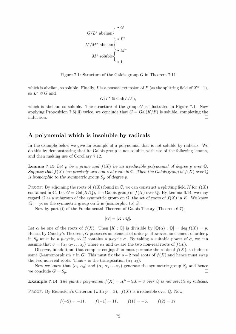
rrrr

1

M∗

L∗

G

M∗ soluble

L∗/M∗ abelian

G/L∗ abelian

Figure 7.1: Structure of the Galois group G in Theorem 7.11

which is abelian, so soluble. Finally, L is a normal extension of F (as the splitting field of Xp−1),so L∗ P G and

G/L∗ ∼= Gal(L/F ),

which is abelian, so soluble. The structure of the group G is illustrated in Figure 7.1. Nowapplying Proposition 7.6(iii) twice, we conclude that G = Gal(K/F ) is soluble, completing theinduction.

A polynomial which is insoluble by radicals

In the example below we give an example of a polynomial that is not soluble by radicals. Wedo this by demonstrating that its Galois group is not soluble, with use of the following lemma,and then making use of Corollary 7.12.

Lemma 7.13 Let p be a prime and f(X) be an irreducible polynomial of degree p over Q.Suppose that f(X) has precisely two non-real roots in C. Then the Galois group of f(X) over Qis isomorphic to the symmetric group Sp of degree p.

Proof: By adjoining the roots of f(X) found in C, we can construct a splitting field K for f(X)contained in C. Let G = Gal(K/Q), the Galois group of f(X) over Q. By Lemma 6.14, we mayregard G as a subgroup of the symmetric group on Ω, the set of roots of f(X) in K. We know|Ω| = p, so the symmetric group on Ω is (isomorphic to) Sp.

Now by part (i) of the Fundamental Theorem of Galois Theory (Theorem 6.7),

|G| = |K : Q|.

Let α be one of the roots of f(X). Then |K : Q| is divisible by |Q(α) : Q| = deg f(X) = p.Hence, by Cauchy’s Theorem, G possesses an element of order p. However, an element of order pin Sp must be a p-cycle, so G contains a p-cycle σ. By taking a suitable power of σ, we canassume that σ = (α1 α2 . . . αp) where α1 and α2 are the two non-real roots of f(X).

Observe, in addition, that complex conjugation must permute the roots of f(X), so inducessome Q-automorphism τ in G. This must fix the p− 2 real roots of f(X) and hence must swapthe two non-real roots. Thus τ is the transposition (α1 α2).

Now we know that (α1 α2) and (α1 α2 . . . αp) generate the symmetric group Sp and hencewe conclude G = Sp.

Example 7.14 The quintic polynomial f(X) = X5 − 9X + 3 over Q is not soluble by radicals.

Proof: By Eisenstein’s Criterion (with p = 3), f(X) is irreducible over Q. Now

f(−2) = −11, f(−1) = 11, f(1) = −5, f(2) = 17.

72

Hence, by the Intermediate Value Theorem, f(X) has at least three real roots (one between−2 and −1, one between −1 and 1 and one between 1 and 2). The derivative of f(X) is

f ′(X) = 5X4 − 9,

so f ′(X) has exactly two real roots, so f(X) has two turning points. There must be a turningpoint between every pair of real roots (Rolle’s Theorem), so f(X) has exactly three real rootsand therefore two non-real roots. Now Lemma 7.13 tells us that

GalF (f(X)) ∼= S5,

the symmetric group of degree 5. Now the alternating group A5 is a non-abelian simple groupand is therefore not soluble. Hence, using Proposition 7.6(i), the Galois group of f(X) over Qis not soluble and, by Corollary 7.12, f(X) is not soluble by radicals.

Thus for this particular quintic polynomial, we cannot express the roots using formulaeinvolving field operations and pth roots.

Galois’s Great Theorem

We finish the chapter by establish the converse of Corollary 7.12; that is, we shall show thatif the Galois group of a polynomial is soluble then the polynomial is soluble by radicals. Webegin with a special case in Lemma 7.16, which can be viewed as a base step of an inductionargument, but we first need a technical result in the middle.

Lemma 7.15 Let K be a finite normal extension of a field F of characteristic zero, let ε ∈ Fand suppose that Gal(K/F ) is cyclic of order p generated by some F -automorphism φ. Thenthere exists some x ∈ K such that

x+ ε(xφ) + ε2(xφ2) + · · ·+ εp−1(xφp−1) 6= 0.

Proof: We actually prove a stronger assertion: Namely we claim that there does not existnon-zero scalars λ0, λ1, . . . , λp−1 in K such that

λ0x+ λ1(xφ) + · · ·+ λp−1(xφp−1) = 0

for all x ∈ K. Suppose for a contraduction that such non-zero scalars λi exist. Choose n to beas small as possible such that there exist non-zero λ0, λ1, . . . , λn ∈ K with

λ0x+ λ1(xφ) + · · ·+ λn(xφn) = 0 (7.4)

for all x ∈ K. Our assumption ensures n 6 p− 1, while n > 1 since K is a field.Since n 6 p− 1, the automorphism φn is not the identity and so we can choose y ∈ K with

yφn 6= y. Note that successive application of φ permutes the elements of y, yφ, yφ2, . . . , yφp−1in a cycle of length p. In particular, since p is prime, these elements must be distinct.

Substitute yx for x in the above equation (7.4). We use the fact that φ and all its powersare automorphisms to conclude

λ0yx+ λ1(yφ)(xφ) + · · ·+ λn(yφn)(xφn) = 0 (7.5)

for all x ∈ K. Now multiply Equation (7.4) by yφn and subtract Equation (7.5) to deduce

λ0(yφn − y)x+ λ1(yφn − yφ)(xφ) + · · ·+ λn−1(yφn − yφn−1)(xφn) = 0

73

for all x ∈ K. Since the images of y under the powers of φ are distinct, the coefficients µi =λi(yφ

n − yφi) are non-zero and we now have an equation

µ0x+ µ1(xφ) + · · ·+ µn−1(xφn) = 0

for all x ∈ K. This contradicts our minimality choice of n.In conclusion, there does not exist non-zero scalars λi satisfying

λ0x+ λ1(xφ) + · · ·+ λp−1(xφp−1) = 0

for all x ∈ K. In particular, taking λi = εi, there exists some x ∈ K such that

x+ ε(xφ) + · · ·+ εp−1(xφp−1) 6= 0.

Lemma 7.16 Let K be a finite normal extension of a field F of characteristic zero and supposethat Xp− 1 splits in F (for some prime p). If Gal(K/F ) is cyclic of order p then K = F (α) forsome α satisfying αp ∈ F .

Thus the lemma shows that, under the given hypotheses, K is a simple radical extensionof F .

Proof: By the Theorem of the Primitive Element (Theorem 4.11), K = F (β) for some β ∈ F .We know that the roots of Xp − 1 in K are 1, ε, ε2, . . . , εp−1 for some ε ∈ F . Let φ be agenerator for G = Gal(K/F ). Use Lemma 7.15 to produce x ∈ K such that

α = x+ ε(xφ) + ε2(xφ2) + · · ·+ εp−1(xφp−1) 6= 0.

Then, noting εφ = ε since φ is an F -automorphism and ε ∈ F ,

αφ = xφ+ ε(xφ2) + ε2(xφ3) + · · ·+ εp−1x = ε−1α,

so(αp)φ = (αφ)p = (ε−1α)p = αp.

Hence αp ∈ FixK(G) = F (by Lemma 6.8).Since ε 6= 1 and α 6= 0, we have αφ 6= α, so α /∈ F . Thus

F $ F (α) ⊆ K.

Now by part (i) of the Fundamental Theorem of Galois Theory (Theorem 6.7),

|K : F | = |G| = p

so, using the Tower Law, F (α) = K, as required.

Theorem 7.17 (Galois’s Great Theorem) Let f(X) be a polynomial over a field F of char-acteristic zero. Then f(X) is soluble by radicals if and only if the Galois group of f(X) over Fis soluble.

Proof: One direction of this theorem is, of course, already established as Corollary 7.12. Itremains to establish the converse.

Let K be the splitting field of f(X) over F and assume that G = Gal(K/F ) is a solublegroup. We shall establish the existence of a radical extension of F that contains the splittingfield K. We proceed by induction on the order of G. If G = 1, then K = F (by part (i) of

74

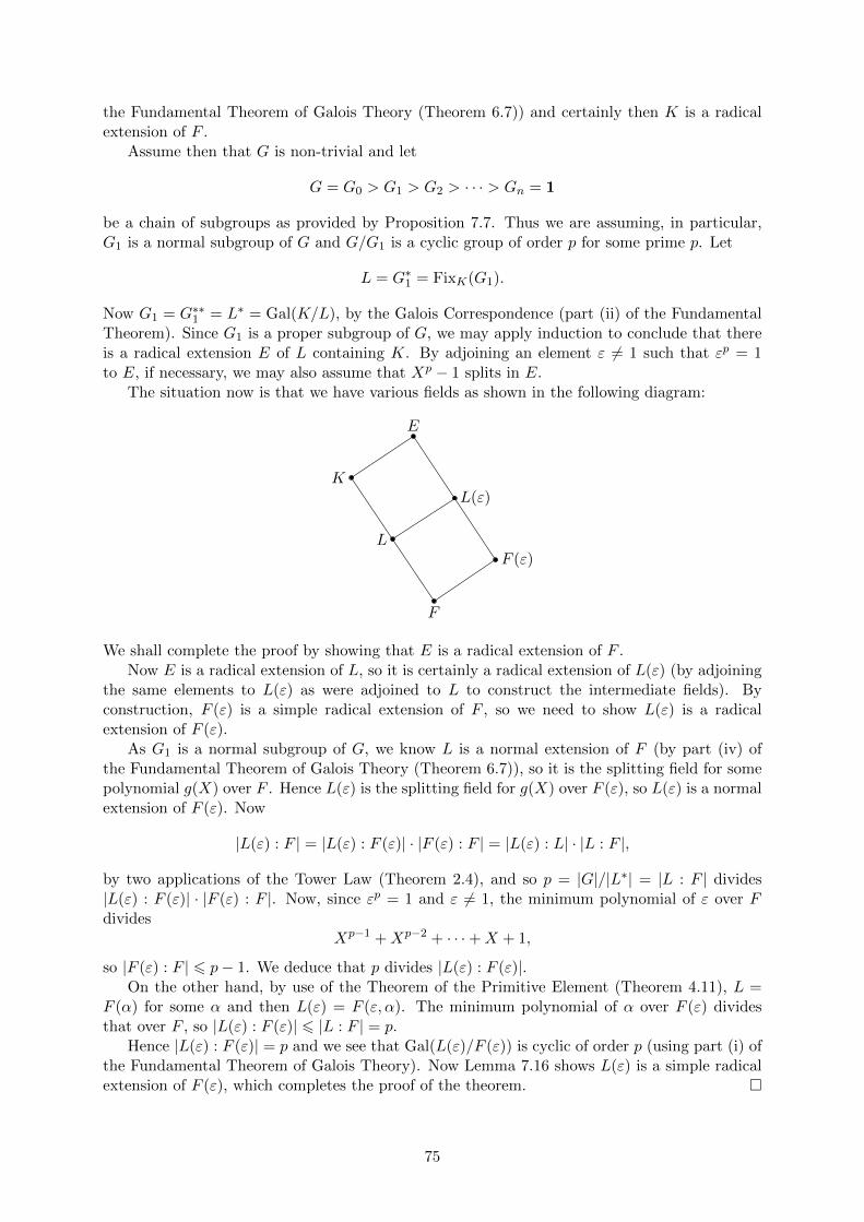
the Fundamental Theorem of Galois Theory (Theorem 6.7)) and certainly then K is a radicalextension of F .

Assume then that G is non-trivial and let

G = G0 > G1 > G2 > · · · > Gn = 1

be a chain of subgroups as provided by Proposition 7.7. Thus we are assuming, in particular,G1 is a normal subgroup of G and G/G1 is a cyclic group of order p for some prime p. Let

L = G∗1 = FixK(G1).

Now G1 = G∗∗1 = L∗ = Gal(K/L), by the Galois Correspondence (part (ii) of the FundamentalTheorem). Since G1 is a proper subgroup of G, we may apply induction to conclude that thereis a radical extension E of L containing K. By adjoining an element ε 6= 1 such that εp = 1to E, if necessary, we may also assume that Xp − 1 splits in E.

The situation now is that we have various fields as shown in the following diagram:

F

L

K

E

L(ε)

F (ε)

We shall complete the proof by showing that E is a radical extension of F .Now E is a radical extension of L, so it is certainly a radical extension of L(ε) (by adjoining

the same elements to L(ε) as were adjoined to L to construct the intermediate fields). Byconstruction, F (ε) is a simple radical extension of F , so we need to show L(ε) is a radicalextension of F (ε).

As G1 is a normal subgroup of G, we know L is a normal extension of F (by part (iv) ofthe Fundamental Theorem of Galois Theory (Theorem 6.7)), so it is the splitting field for somepolynomial g(X) over F . Hence L(ε) is the splitting field for g(X) over F (ε), so L(ε) is a normalextension of F (ε). Now

|L(ε) : F | = |L(ε) : F (ε)| · |F (ε) : F | = |L(ε) : L| · |L : F |,

by two applications of the Tower Law (Theorem 2.4), and so p = |G|/|L∗| = |L : F | divides|L(ε) : F (ε)| · |F (ε) : F |. Now, since εp = 1 and ε 6= 1, the minimum polynomial of ε over Fdivides

Xp−1 +Xp−2 + · · ·+X + 1,

so |F (ε) : F | 6 p− 1. We deduce that p divides |L(ε) : F (ε)|.On the other hand, by use of the Theorem of the Primitive Element (Theorem 4.11), L =

F (α) for some α and then L(ε) = F (ε, α). The minimum polynomial of α over F (ε) dividesthat over F , so |L(ε) : F (ε)| 6 |L : F | = p.

Hence |L(ε) : F (ε)| = p and we see that Gal(L(ε)/F (ε)) is cyclic of order p (using part (i) ofthe Fundamental Theorem of Galois Theory). Now Lemma 7.16 shows L(ε) is a simple radicalextension of F (ε), which completes the proof of the theorem.

75