1

On the Relationship Between Environmental and Macroeconomic Policy.

October, 2019

PRELIMINARY DRAFT: PLEASE DO NOT QUOTE.

Nicholas Z. Muller Carnegie Mellon University

National Bureau of Economic Research Wilton E. Scott Institute for Energy Innovation

Abstract

This paper explores the relationship between environmental policy and macroeconomic policy. The link hinges on a redefinition of output that deducts pollution damage from Gross Domestic Product. The paper proposes a dual link through the object of stabilization policy, consumption volatility, and stabilization tools, interest rates. Volatility in pollution-adjusted consumption depends on the covariance of market goods and services and pollution damage. The nature of the covariance hinges on the stringency of pollution control. Pollution-adjusted interest rates depend on the intertemporal changes in pollution intensity. Economies on a cleaning-up path justify a higher natural rate. Societies growing more pollution intensive suggest a lower natural rate. In an empirical application to the U.S. economy, the natural rate inclusive of pollution damages differs significantly from the federal funds rate. The implementation of major federal air pollution legislation enacted in the 1970s significantly affected the covariance between damages and output. The effect of this on year-over-year variance in per capita consumption, net of pollution damage, is appreciable. Keywords: Natural interest rate, stabilization, air pollution, greenhouse gases, environmental accounting. JEL Codes: E43, E63, E21, Q53, Q54, Q56, Q58, Q51.

2

I. Introduction.

Macroeconomic policymakers rely on the National Income and Product Accounts (NIPAs) for

estimates of real output and growth, both of which are important determinants of efforts to

stabilize, and more broadly, manage, economic and financial systems. Yet, the NIPAs are

incomplete. The NIPAs omit three key contributors to national economic welfare: the value of

leisure time, home production, and environmental goods and services (Nordhaus and Tobin,

1973; NAS NRC, 1999). The present paper demonstrates that the third omission has large and

measureable consequences for metrics critical to macroeconomic policy: volatility in per capita

consumption and the natural interest rate.

To show that extending the NIPAs to include the environment has repercussions for

macroeconomic policy, the paper introduces an adjusted measure of consumption grounded in

the national accounting literature (Nordhaus and Tobin, 1973; Nordhaus, 2006; Abraham and

Mackie, 2006; Muller, 2014). In accord with this literature, pollution damage is deducted from

Gross Domestic Product (GDP) to measure net or environmentally adjusted value-added (EVA)

since emissions are an unpriced residual from market production and consumption1.

In contrast to prior analyses of environmentally-adjusted accounts that focus on sectoral

decompositions (Muller, Mendelsohn, and Nordhaus, 2011; Tschofen et al., 2019), growth

(Muller, 2014; 2019b), or discounting (Muller, 2019a), the present focus lies at the intersection

1 The presence of environmental regulation may give one pause as to whether such costs are already in the accounts. Note, however, that what is subtracted are damages from remaining emissions, net of environmental policy. The only case in which double counting would occur is if emissions are taxed according to their marginal damages (or if firms, subject to a system of tradable permits, had to purchase all allowances in an auction format). U.S. environmental regulations take the form of standards as well as a collection of small-scale or regional cap-and-trade programs that, for the most part, grant allowances for free.

3

of environmental and macroeconomic stabilization policies. The paper proposes a dual link. One

connection occurs through the object of stabilization: consumption volatility. The other relation

manifests through tools to achieve stabilization: interest rates.

With pollution damage deducted from market consumption, volatility in EVA depends not just

on the variance of its parts but also on their co-movements2. Positive covariance between

damage and market consumption dampens volatility in EVA since the covariance term enters the

expression for the variance of a difference of random variables negatively. However, negatively

covariant damages and output accentuate volatility. Importantly, the sign of the covariance

between market consumption and pollution damage hinges on environmental policy. Absent

aggressive environmental policy, this covariance is likely positive. Greenhouse gases and most

major air pollutants are produced from the combustion of fossil fuels from power production,

manufacturing processes, transportation, and agriculture. Hence, more economic output, absent

abatement, translates to more emissions. Upon implementation of binding environmental

controls, the covariance term may attenuate or become negative. Environmental policy affects

volatility in consumption through the sign of the relationship between market output and

damage.

Using the redefinition of potential income (inclusive of pollution damages) proposed above,

pollution damages also affect interest rates. This connection is most clearly evident if one

considers a definition of the natural interest rate. Laubach and Williams (2015) define the natural

rate as “the real short-term interest rate consistent with the economy operating at its full

potential.” Similarly, Goodfriend (2016) states that “the natural interest rate is the interest rate

that makes desired aggregate lifetime consumption plans conform to present and expected future

2 Recall that the variance of a difference of two random variables is: Var(X – Y) = var(X) + var(Y) – 2cov(X,Y)

4

potential output…” The contention herein is that “potential” or “full potential” income is

fundamentally mis-measured without consideration of environmental pollution damage3. The

empirical analysis conducted in this paper demonstrates that environmental policy affects

pollution damages and, thus, the level of potential output. This forges the connection between

natural interest rates and environmental policy.

The connection between environmental quality and full potential income, a key driver of the

natural interest rate, may seem oblique. To concretize this mechanism, consider that since the

1970’s, empirical research reports an association between exposure to environmental air

pollutants and premature mortality (Lave and Seskin, 1970; Dockery et al., 1993; Krewski et al.,

2009; Lepeule et al., 2012)4. Further, a range of morbidity (illness) states are also amplified by

exposures to environmental pollutants (USEPA, 1999; 2010). Thus, both the size (through

mortality risk) and the productivity (through illness and absenteeism) of the labor force are

plausibly affected by environmental exposures. Hence the link between pollution exposure,

damage, and potential output.

The empirical section of the paper employs carbon dioxide (CO2) and air pollution damage

estimates spanning from 1957 to 2016 in the U.S. economy. The air pollution series (developed

in Muller, 2019b), reports estimates of premature mortality risk from exposure to fine particulate

matter (PM2.5) on an annual, aggregate (across the U.S.) basis. The CO2 series uses U.S.

Department of Energy emission estimates along with the social cost of carbon to tabulate

greenhouse gas damage (USDOE, 2011; 2019; USFWG, 2016). The 60-year time horizon in this

study encompasses years before and after the passage and implementation of landmark federal

3 The position that mis-measurement of potential income will yield mischaracterization of the natural interest rate is also noted in Laubach and Williams (2015), though not due to environmental hazards. 4 In addition to the epidemiological literature, recent research in environmental economics reports significant causal impacts of exposure to PM2.5 on adult mortality rates (Jha and Muller, 2018; Deryugina et al., 2019).

5

legislation to control air pollution. (The Clean Air Act was passed in 1970, and implemented in

the years following.) The period also includes several recessions and, hence, considerable

variation in macroeconomic conditions. The empirical setting provides an excellent opportunity

to test how pollution-adjusted measures of consumption volatility and natural interest rates

change relative to environmental policy and the business cycle.

a. Preview of Results.

The conceptual modeling confirms the links between environmental pollution damages (and

hence, environmental policy) and macroeconomic policy proposed above. The first result

pertains to volatility in the augmented measure of per capita consumption. The conceptual model

introduces uncertainty in both future market consumption and pollution damage. Doing so

confirms that volatility in EVA is the sum of the variances of consumption of market goods and

services and pollution damage less their covariance. The empirical analysis shows that the

variance of EVA was less than GDP prior to passage of the Clean Air Act. During this pre-policy

period, GDP and pollution damages were positively correlated. Following enactment of the Act,

volatility in EVA exceeded that of GDP because of the significant negative covariance between

GDP and damages. Thus, the sign of the covariance hinges on the stringency of pollution control.

This critically affects the relative volatility of EVA and GDP.

The second result pertains to the calibration of the natural interest rate. When potential income

reflects the deduction of pollution damage, the pollution-adjusted rate (hereafter, the green

interest rate) depends on the intertemporal changes in pollution intensity. Economies on a

cleaning-up path justify a higher rate. Societies growing more pollution intensive suggest a lower

rate. The intuition for this orientation is the following. In economies becoming cleaner, or less

pollution intensive, current prospects for future consumption brighten. Thus, delaying present

6

consumption so that it occurs when less environmental pollution damage is deducted from

market consumption enhances welfare. Higher rates induce savings and investment, encouraging

more future consumption relative to that in the present. Conversely, if an economy is degrading

its environment, expectations for future consumption prospects become dimmer; consumption in

the future suffers a greater implicit tax stemming from higher losses due to pollution damage.

Under such conditions, the interest rate should fall, reducing the incentive to save. Consuming

more in the present attenuates the effective penalty from pollution damage.

The paper empirically compares the green interest rate to the federal funds rate. On average, the

green interest rate exceeded the federal funds rate by 50 basis points. However, the green interest

rate was less than the federal funds rate from 1957 to 1970. This occurred because pollution

intensity and damages were on the rise, dampening future consumption prospects. The lower

green rate encourages more near-term consumption at the expense of future consumption when

the pollution penalty (the deduction of damage from potential income) was higher. Following

1970, the green interest rate exceeded the federal funds rate because combined CO2 and air

pollution damage fell over the 1970 to 2016 time period. Hence, a relatively higher interest rate

induces less near-term consumption and slightly more in the future when pollution damage is

lower.

In a simulation exercise, the analysis models intertemporal changes to consumption and savings

that would occur if households faced the green interest rate. In total, the intertemporal

reallocation of consumption induced by the green interest rate would have prevented between

7,000 and 25,000 premature deaths from PM2.5 exposure. Importantly, the vast majority of these

benefits would have occurred immediately following passage and prior to full enactment of the

Clean Air Act. While these reductions are a small fraction of total damages, and of the emission

7

changes induced by the Clean Air Act, this new environmental-macroeconomic policy dimension

could have provided an important stopgap prior to the full enactment of the Clean Air Act.

The remainder of the paper is structured as follows. Section II introduces the conceptual model

and works through the alternative definitions of consumption, interest rates, the intertemporal

consumption path, and volatility in consumption. Section III presents the data and methods.

Section IV covers results and V concludes.

II. Model.

This section of the paper begins by laying out the basic conceptual modeling set up and

establishing the alternative definitions of consumption. Next it derives expressions for the

interest rates using each measure of consumption and the resulting intertemporal consumption

paths. Finally, the conceptual model introduces uncertainty in labor productivity and pollution

intensity.

a. Basic Set-Up

Assume the economy is comprised of identical consumers that seek to maximize lifetime utility

derived from consumption in a two period model: 𝑈(𝑐 , 𝑐 ) = 𝑢(𝑐 ) + 𝑢(𝑐 ), where (ct) is

consumption of market-produced goods in period (t), and the pure rate of time preference is

given by (𝜌). More specifically, let 𝑈(𝐶 ) = , denote utility from consumption in period

(t)5. As is well-known, the present value of lifetime utility is maximized when the marginal

utility from consumption, again in present value terms, is equated across time periods and

5 The appendix explores a constant elasticity of substitution utility function defined over environmental quality and market goods.

8

consumers utilize their entire budget. And, with power utility, because consumers can borrow

and lend at (r), the extant real interest rate, this condition is shown in (1):

= (1)

Hence, the marginal rate of substitution is equated to (one plus) the interest rate, discounted.

Following Goodfriend (2004; 2016), let , reflect potential income in periods

(1) and (2), respectively. The (𝜇 ) term in the denominator reflects distortions that attenuate

potential income such a taxes, regulations and the like. The (𝛾 ) term represents expenditures on

environmental quality (i.e. pollution control). Plugging in to (1), for (c2), and

rearranging yields an expression for current consumption: 𝑐 = .

The same notation for period (1) potential output obtains:

= (2)

Thus, consumption across the two periods equals potential income. Ultimately, (2) is solved for

(r), the interest rate that maximizes two-period consumption. The next subsection introduces

pollution into potential income.

a. Alternative definitions of potential income.

In addition to the market-centric definition of potential income above, this paper includes both

investments in environmental quality (pollution control) and damages from pollution. As above,

in period (t), 𝛾 depicts the fraction of income allocated to pollution control; investments in

9

abatement of environmental pollutants such as CO2 or particulate matter. Next, let 𝛼 denote the

pollution intensity of output, say CO2 damage per unit GDP, and 𝛽 shows the responsiveness of

environmental pollution damage to abatement investment 𝛾 .

Therefore, maximum potential income in period (1) is redefined as shown in (3):

𝑐 =( )

(3)

Here, the superscript (e) denotes “environmentally-adjusted” consumption. Note that abatement

expenditure (𝛾 ) reduced damage through (𝛽 ) and it deducts from potential income through the

denominator of (3).

b. Interest Rates.

The analysis next turns to interest rates. The thrust of this section is to characterize differences in

interest rates with and without acknowledgement of non-market pollution damages. This section

solves for the two-period consumption maximizing interest rate beginning with deterministic

consumption measures. Section II.d introduces uncertainty in productivity and pollution intensity

and the implications of this for volatility in consumption as defined in (3).

To begin, (2) is solved for (r). This yields the natural interest rate; that which equates

consumption in each period to maximum potential output. For simplicity, we assume 𝜂 = 1.

This yields (4):

𝑟 = (1 + 𝜌) − 1 (4)

10

Hence, the natural rate of interest is increasing in the growth of potential income (labor

productivity) and in households’ rate of time preference and it is attenuated by income-reducing

distortions.

Substituting (3), the pollution-adjusted measure of consumption into (2) and solving for (r) yields

(5):

𝑟 = (1 + 𝜌)( )

( )− 1 (5)

Expression (5) is the green interest rate.

Of particular interest is the final term: ( )

( ). This is the ratio of pollution intensity

across the two periods. That is, 𝑌 (𝛼 − 𝛽 𝛾 ) characterizes period (1) monetary pollution

damage, and 𝑌 1 − (𝛼 − 𝛽 𝛾 ) depicts period (1) net potential income. Hence, (1 −

(𝛼 − 𝛽 𝛾 )) conveys the pollution intensity of the economy in period 1; higher values of (1 −

(𝛼 − 𝛽 𝛾 )) indicate lower pollution density of output, given abatement. Thus, the ratio

( )

( ) shows how environmental pollution damage intensity changes across the two

time periods.

As is clear in (5), the direction of change in pollution damage is crucial to determining the green

interest rate. An economy on a “cleaning-up” trajectory features ( )

( )> 1.

Conversely, an economy with rising pollution intensity suggests: ( )

( )< 1. If

( )

( )> 1, the reduction in future damages boosts consumption prospects in the future,

and the interest rate in (5) will be higher than (4). As demonstrated below, the higher green

11

interest rate (when pollution damages are falling) induces more savings, less consumption today,

and more consumption in the future. More consumption occurs when the economy is “cleaner”,

or pollution intensity is lower.

However, when ( )

( )< 1, pollution intensity is rising; this dampens the green interest

rate because rising damage implies more limited consumption opportunities (lower potential

income) in the future. A lower green interest rate due to rising damages draws consumption from

the future into the present when the drag due to pollution damage is lower.

Expression (5) and the subsequent discussion forge the first link between environmental policy

and macroeconomic policy in this paper. Specifically, the stringency of environmental policy

clearly influences the net intensity of pollution damage. Intertemporal changes in net pollution

intensity are transmitted through the green interest rate to affect intertemporal consumption

decisions.

Mismeasurement of income potential, and by extension income growth, results in

mischaracterization of the natural interest rate (Laubach and Williams, 2015). In the present

context, mismeasurement occurs by omission of non-market pollution damage and changes in

pollution intensity over time. Expression (6) shows the measurement error implicit in the natural

interest rate due to omitting environmental pollution damage.

Δ = 𝑟 − 𝑟 = (1 + 𝜌)( ) ( )

( ) (6)

The difference in rates is positive if pollution intensity is falling. Conversely, (r1) exceeds the

green interest rate if damages are rising. There is no mismeasurement if pollution intensity is

static between the two time periods. Expression (6) also reveals that the difference in rates is

12

increasing in the degree to which the economy is polluted in period 1; the difference becomes

arbitrarily large as (𝛼 − 𝛽 𝛾 ) → 1. In this extreme case, the (environmental, or social) penalty

to consumption in the present becomes infinitely large.

c. The Consumption Path.

The model next considers how the interest rates (r1) and (rg) affect environmentally-adjusted

consumption in the two period model. To accomplish this, the expressions for (𝑐 , 𝑐 ) are

evaluated at (r1) and (rg), for the case of log utility.

Deducting 𝑐 (𝑟 ) from 𝑐 𝑟 yields (7):

Δ , = 𝑐 𝑟 − 𝑐 (𝑟 ) =( ) ( )

( ) (7)

This expression indicates that the difference in period (1) consumption, according to whether

households face (r1) or (rg), hinges on whether pollution intensity of output is rising or falling. In

an economy with rising pollution intensity, Δ , > 0. Consumption tilts to the present if households

face (rg) rather than (r1). This should be intuitive. An economy growing more polluted levies a

larger effective tax on consumption in the future. That is, a greater share of consumption is lost to

pollution damage in the future period relative to the present. Interest rates should convey these

expected conditions to consumers. This is precisely the signal that (rg) presents, relative to (r1).

In the opposite case, in which pollution intensity is falling, Δ , < 0. Consumption tilts to the future

if consumers face the green interest rate relative to (r1). This occurs because with less distortion

from pollution in period (2), it is preferred for households to consume less in the present and more

in the less-polluted context of period (2). The higher green interest rate presents consumers with

this incentive. And, trivially, if pollution intensity is constant: Δ , = 0.

13

Repeating this experiment for period (2), produces the following expression for the difference in

consumption given (r1) and (rg):

Δ , = 𝑐 𝑟 − 𝑐 (𝑟 ) =( ) ( )

( ) (8)

Expression (8) presents the mirror image of (7). With rising (falling) pollution intensity,

consumption in period (2) subject to (rg) falls short of (exceeds) that conditional on (r1). The

intuition of this permutation of consumption in period (2) given (rg) relative to (r1) is presented

above.

Of course, whether or not policymakers target the natural rates defined by (r1) or (rg) also has

implications for the consumption growth rate. Specifically, evaluating 𝑐 and 𝑐 according to (r1)

or (rg), then computing the proportional growth rates in consumption produces (9) and (10).

𝐺 =( ) ( )

( ) ( )− 1 (9)

𝐺 =( ) ( )

( ) ( )− 1 (10)

In (9), which relies on the natural rate of interest absent environmental damage, growth of

consumption is increasing (decreasing) if pollution damage intensity is rising (falling). This sub-

optimal consumption path stems from the mismeasurement of consumption in the expression for

(r1). In contrast, (10) shows that the green interest rate induces a higher growth rate when pollution

damage is falling. This comports with the logic laid out above.

The consumption path induced by (r1) is demonstrably sub-optimal. The first-order condition for

optimal inter-temporal consumption equates the marginal rate of substitution between

consumption in periods (1) and (2) to . Evaluating marginal utilities at (𝑐 , 𝑐 ), which follow

14

from the green interest rate (rg), and computing the ratio yields: ( )

( ), or

. Conversely, computing marginal utilities at the levels of consumption induced by (r1), and

computing the ratio yields: ( )

( )≠ . The key difference lies in the

last terms: ( )

( ) and

( )

( ).

Figure 1 shows these different paths. The two linear downward sloping lines represent budget

constraints. The outer constraint corresponds to apparent feasible consumption paths. The inner

constraint deducts environmental pollution damage. Note the difference in slopes. The slope of the

outer constraint is , whereas the slope of the inner constraint is: . In this configuration,

𝑌 (𝛼 − 𝛽 𝛾 ) > 𝑌 (𝛼 − 𝛽 𝛾 ). Damages are falling. As demonstrated above, when damages fall

from period 1 to period 2, the consumption path incentivized by features more consumption

in period 1 and less in period 2 than the path induced by . This is shown on figure 1 by the

point B, relative to the tangency condition at (𝑐 , 𝑐 ). At point B, consumers equate their MRS to

, inducing a suboptimal intertemporal consumption path.

Summarizing this subsection, interest rates based on measures of output that omit damage yield

suboptimal consumption paths. The orientation of this sub-optimality hinges on whether pollution

intensity is rising or falling. An economy on a cleaning-up trajectory will feature too much near

term consumption if interest rates are defined without consideration of pollution. Conversely, in

an economy becoming dirtier, too much savings occurs.

15

d. Uncertainty in Productivity, Pollution, and Consumption.

While uncertainty is likely to permeate each aspect of this model, the focus is on uncertainty in

productivity growth and pollution intensity growth. (One motivation for not exploring uncertainty

in abatement intensity is that environmental policy targets are often pre-specified, or codified, in

extant policies.) In accord with the notation above, let expected productivity in period (t) = (𝑌 ),

and the expected pollution intensity in period (t) = (𝛼 ). Time period (t) additive shocks to these

two rates are given by (𝜀 , ) and (𝜀 , ). In terms of the distribution of these shocks, it is assumed

that Ε(𝜀 ) = 0, and Ε(𝜀 ) = 0; Ε(𝜀 ) = 𝜎 ; Ε(𝜀 ) = 𝜎 ; Ε 𝜀 𝜀 = 𝜌 , . Thus, the period (t)

realization of productivity is: 𝑌 + 𝜀 , ; and that for pollution intensity is; 𝛼 + 𝜀 , . In this setting,

the period (2) equivalent of (2) and (3) with uncertainty is given by (11) and (12):

𝑐 =

(11)

𝑐 =

(12)

From an ex ante perspective, the policymaker is not equipped with sufficient information to set the

optimal rate (either (𝑟 ) or (𝑟 )) conditional on realized productivity and pollution shocks. The

policymaker’s second best choice is to regulate according to their expectations over productivity

and pollution shocks. According to this tack, and because of the mean-zero property of the

distribution of pollution and productivity shocks, the regulator employs the deterministic

characterizations of (𝑟 ) or (𝑟 ) shown in (4) and (5).

16

A primary goal of macroeconomic policy is limiting volatility in consumption. A key reason for

this policy objective is that excessive variability in economic conditions is costly (Lucas, 1981).

The analysis first characterizes the variance in future consumption for both (11) and (12). In

examining the variance in future consumption, (11) and (12) are evaluated at (r1) and (rg),

respectively.

Expression (13) presents the variance in consumption absent pollution damage.

𝑣𝑎𝑟 𝑐 = 𝜎 =( )

(13)

Straightforwardly, the variance in future market consumption depends on the variation in future

productivity shocks.

The value of expression (13) is in comparison with (14) below, which depicts the variance in

augmented consumption.

𝑣𝑎𝑟(𝑐 ) = 𝜎 =( )

𝜎 1 − (𝛼 − 𝛽 𝛾 ) + 𝜎 (𝑌 + 𝜀 ) − 2𝜌 , 1 − (𝛼 − 𝛽 𝛾 )

(14)

While this expression may seem cumbersome, it is quite intuitive, given how augmented

consumption is defined. The form in (14) stems from the fact that augmented consumption is

market consumption less pollution damage. Hence, it is the variance of a difference of random

variables. This structure yields a well-known general form: the sum of variances less the

covariance of the random variables6.

6 Specifically: Var(X – Y) = var(x) + var(y) – 2cov(X,Y).

17

The first term (inside the parenthesis) indicates that the variance in productivity shocks affects

the variance in this measure of consumption through (one minus) the damage intensity of output.

Hence, it is the variance in productivity shocks times the marginal productivity net of damage.

The second term is the variance in pollution intensity shocks. This term is scaled by period (2)

productivity. This means that the contribution of variance in pollution shocks to variance in

consumption is increasing in productivity. Finally, the covariance between pollution and

productivity affects the variance of augmented consumption through marginal productivity net of

damage, akin to the productivity shock. Whether (14) exceeds or is less than variance in market

consumption (13) critically depends on the sign and the magnitude of the covariance term. If

damage and market consumption are negatively correlated, then (14) likely exceeds the variance

in market output. If damage and market consumption are positively correlated, then the

magnitude of (14) relative to (13) is ambiguous.

Of central importance to the covariance between pollution and productivity shocks is abatement.

That is, absent efforts to reduce emissions, one might conjecture that abnormally productive

periods would occur together with high pollution episodes. However, pollution controls limiting

particularly high realizations of (𝜀 ), or even inducing predominantly negative pollution shocks,

may result in negative covariance. Thus, variance in augmented consumption relative to that of

market consumption depends heavily on the presence and stringency of pollution control policy.

III. Data and Methods.

The empirical analysis conducted in this paper relies on several sources of data. These data are

subdivided into two groups: macroeconomic data and environmental data. Section III.a focuses on

the environmental data while III.b discusses sources and methods for the macroeconomic data.

18

a. Environmental pollution data.

The local air pollution series covers annual average fine particulate matter (PM2.5) estimates

reported in Muller (2019b). These data correspond to a combination of satellite observations and

modeled data from 1980 – 2016 provided by Meng et al., (2019), see figure A.1 in the appendix.

For the earlier data, the analysis relies on imputed PM2.5 from total suspended particulate matter

(TSP) data gathered from the early air pollution monitoring networks. The TSP data are provided

by Clay et al., (2016). The imputation, discussed at length in Muller (2019a), regresses observed

PM2.5 in the U.S. Environmental Protection Agency’s AQS monitor network from 1999 to 2016

on matching (spatially and temporally) TSP data. Predictions of PM2.5 are made from 1979 back

to 1957 and this series is spliced with the 1980-2016 satellite series to produce a continuous

PM2.5 series from 1957 to 2016 (see figure A.2).

Conversion of ambient PM2.5 estimates into monetary damage relies on an approach that is

standard in policy analyses (USEPA, 1999; 2010) and in the academic literature (Levy, Baxter,

Schwartz, 2009; Muller, Mendelsohn, Nordhaus, 2011; Muller, 2014). The damages are limited

to premature mortality risk from exposure to PM2.5 both because of historic data constraints and

because prior research in this area has repeatedly demonstrated that this category of damage

accounts for the majority of all air pollution damage (USEPA, 1999; 2010).

Calculation of mortality damage requires vital statistics going back to 1957. The Centers for

Disease Control and Prevention (CDC) provide population and mortality rate data used in this

analysis. These data are reported by age group. This is an essential component of the empirical

analysis because baseline mortality rates vary considerably over the life-cycle and the functions

that link exposure to mortality risk are multiplicative in nature (Krewski et al., 2009).

19

Using population by age cohort (a), location (i), and time (t), denoted (Popa,t), and baseline

(reported) mortality rates, by (a) and (t), denoted (Ma,t), (CDC, various) premature mortality due

to PM2.5 exposure is computed as shown in (15).

𝑀𝑜𝑟𝑡 , , = 𝑃𝑜𝑝 , , 𝑀 , , 1 − 1𝑒𝑥𝑝 𝜃𝑃𝑀 ,

(15)

The (𝜃) term, which controls the marginal effect on mortality risk from PM2.5 exposure, is

reported in the epidemiological literature (Krewski et al., 2009). Aggregating over age groups

and locations yields an estimate of national premature mortality.

In the air pollution context, mortality risk is commonly monetized using the Value of Statistical

Life (VSL) approach. The VSL is the marginal rate of substitution between money (income) and

mortality risk (Hammit and Robinson, 2011). This tack is used by the USEPA in its benefit-cost

analyses of the Clean Air Act (USEPA, 1999; 2010) and by numerous academic researchers

(Levy, Baxter, Schwartz, 2009; Muller and Mendelsohn, 2009; Fann et al., 2009; Muller, 2014;

2019a; 2019b). It is typical to apply the VSL to all populations within a given time period

uniformly, regardless of income. Thus, monetary damages (D) in period (t) are calculated by

simply multiplying premature mortalities times the VSL, shown as (Vt).

𝐷 = ∑ ∑ 𝑀𝑜𝑟𝑡 , , 𝑉 (16)

A crucial concern in the relatively long-run context of the present paper is that the VSL (Vt)

varies by year according to the reported per capita income. To construct the VSL series over the

60-year span of the present study depends on estimates of the VSL-income elasticity reported in

the literature (Kleckner and Neumann, 1999; Costa, Kahn, 2004; Hammitt, Robinson, 2011). The

present analysis employs the VSLs by decade reported in Costa and Kahn (2004) from 1957 to

20

1980. For the 1980 to 2016 period, the paper begins with the USEPA’s recommended VSL of

$7.4 million ($2006). This VSL is adjusted according to changes in real income using the

USEPA’s 0.4 income elasticity (Kleckner and Neumann, 1999). This series was used in Muller

(2019a). Figure A.3 in the appendix shows how the VSL changes from 1957 to 2016.

Emissions of greenhouse gases (expressed as CO2 equivalents) are provided by the U.S.

Department of Energy (DOE, 2011; 2019). These are economy-wide emission estimates.

Monetization of the CO2 emissions employs the social cost of carbon (SCC) metric. This is the

dollar-per-ton marginal damage of CO2 emissions. This study uses the updated SCC from the U.S.

Federal Inter-Agency Working Group report from 2016 (USFWG, 2016). The annual real rate of

change reported in USFWG (2016) is used to estimate the SCC back to 1957. Both the emissions

and the SCC estimates are depicted in figure A.4.

b. Macroeconomic data.

In order to calculate the interest rate specifications derived in section II., several macroeconomic

datasets are required. National GDP is provided by the U.S. Bureau of Economic Analysis

(USBEA, 2019). The fraction of output allocated to abatement of air pollution is calculated from

the USEPA’s most recent benefit cost analysis of the Clean Air Act (USEPA, 2010). Conversion

from nominal to real values relies on the USBEA’s GDP deflator.

What is the appropriate interest rate to serve as the basis for comparison of the green interest

rate? The empirical analysis begins by using the federal funds rate (FRED, 2019b). Kaplan

(2018) refers to the natural interest rate as the “theoretical federal funds rate at which the stance

of Federal Reserve policy is neither accommodative nor restrictive.” Goodfriend (2016) similarly

links policy rates to the natural interest rate: “Interest rate policy is…about shadowing the natural

21

interest rate.” (Goodfriend, 2016 p.4). Finally, Laubach and Williams (2015) aver that the natural

interest rate is “the real short-term interest rate consistent with the economy operating at its full

potential”. Thus, the empirical calibrations of the green interest rate begin with short term, year-

over-year changes in pollution intensity and comparisons are made to the federal funds rate.

The conceptual model characterizes net, potential income in period (1) as: 𝑌 1 − (𝛼 − 𝛽 𝛾 ) .

In order to compute this environmentally-adjusted measure, the gross external damage (GED)

from air pollution and CO2 are computed and deducted from real GDP, by year, from 1957 to

2016. At the national, or economy-wide, scale, this adjusted measure is referred to as

environmentally-adjusted value added (EVA), (Muller, 2014; 2019a). All macroeconomic

aggregates (GDP, GED, and EVA) are expressed in real, per capita terms.

In the appendix section I. is a detailed description of the methods used to provide an assessment

of the effect that the green interest rate would have on consumption/savings decisions by

households. Briefly, this hinges on consumption responses (and, subsequently, damages) to the

change in interest rates if households faced the green interest rate. The simulation recursively

tracks the change in consumption and damages from 1957 to 2016. In doing so, it also estimates

EVA and EVA growth rates to assess the effect of the green interest rate on adjusted growth.

IV. Results.

The results section begins with a brief description of summary statistics and stylized facts that

are relevant to the analysis that follows. Figure 2 depicts the real GDP, EVA, and GED series

from 1957 to 2016. Real, per capita GDP increased from just under $20,000 in the late 1950s to

nearly $60,000 in 2016. By definition, EVA is always less than GDP, as GED is deducted from

GDP to estimate EVA. Fluctuations and the business cycle are evident in both series. From 1957

22

to 1970, GED increased in concert with GDP. EVA grew less rapidly that GDP over this decade

(Muller, 2019a). However, figure 2 makes clear that since real GED fell from roughly 1970 to

2016, the gap between EVA and GDP narrowed over this 50 year period. Thus, since 1970, EVA

growth seemingly outpaced real, per capita GDP growth.

Table 1 concretizes the results in figure 2. Prior to 1970, air pollution and climate damage

averaged just under $7,000 per capita or about 1/3 of per capita income. This figure (also

reported in Muller, 2019a) reveals a stunningly large external cost burden. Just 7 percent of this

damage was due to CO2 emissions. Table 1 and the left panel of figure 3 reveals that CO2

damage climbed throughout the sample, while air pollution GED started to fall in the 1970’s.

The shares of GED from air pollution and CO2 changed considerably between 1970 and 2016; in

the final decade of the analysis CO2 damage comprises 13 percent of GED.

Table 2 focuses on annual growth rates. Column (1) reports the 60-year average growth rates for

GED, GDP, and EVA. Over the entire period, air pollution damage fell by one half of a

percentage point per year. In contrast, damages from CO2 increased by two percent, annually.

Real, per capita GDP increased by just under two percent per year. Deducting the GED enhances

growth, relative to GDP. Specifically, when GED (including both air pollution damages and

CO2) is deducted from GDP, the EVA growth rate was 2.40 percent, or about half of a

percentage point more rapid than GDP. Table 2 reports considerable heterogeneity in growth of

GED, EVA, and GDP by decade7. The central result from the comparison of growth rates over

time in the U.S. economy is that before 1970, EVA growth fell short of GDP growth, because

GED was growing. Whereas, after 1970 which featured the passage of the Clean Air Act, EVA

7 While Muller (2019a) reported air pollution GED and relative growth metrics for this time period, the present study includes CO2.

23

growth outpaced GDP growth because the air pollution GED fell rapidly (Muller, 2019a). More

specifically, prior to 1970 air pollution GED grew rapidly at about 4 percent annually. CO2

damage was also growing quickly: 3.4 percent per annum. After 1970, air pollution GED

contracted because the local air pollutants comprising GED were regulated by the Clean Air Act.

The maximum rate of decline (2.9 percent) occurred during the 2000’s. In contrast, CO2

continued to expand. This growth in CO2 GED occurred because this pollutant was largely

unregulated throughout the entire sample period.

The difference between EVA and GDP growth, while persistently positive after 1970, narrowed

considerably. During the 1970s, the growth gap averaged about 150 basis points. During the

1980s the spread was roughly 100 basis points. By 2016, the divergence was just 15 basis points.

The growth rate of CO2 and air pollution damage, along with real GDP are shown in the right

panel of figure 3. This graph makes clear the influence of environmental policy on the relative

growth rates of CO2 and air pollution damage. From 1957 to 1970, GED from these two

pollutants increased. Then, upon passage of the Clean Air Act in 1970, the growth rates of GED

from air pollution turned negative. Growth in CO2 damage was typically positive and closely

aligned with GDP. And both air pollution and CO2 damages are clearly sensitive to the business

cycle.

a. Interest rates.

Table 3 reports two different sets of interest rates. As a benchmark for comparison, table 3

reports the federal funds rate (FRED, 2019b). Over the entire sample, the federal funds rate

averaged about 5 percent. As is well known, the federal funds rate fluctuated over this 60-year

period. In the 1960s, the federal funds rate averaged less than four percent. The federal funds rate

24

increased in the 1970s, and peaked in the 1980s, during which time it averaged about 10 percent.

From the 1990s through 2016, the federal funds rate fell. Table 3 also reports the green interest

rate calculated using the expression in (5). Table 3 reports that on average the green rate

exceeded the federal funds rate by about 50 basis points. Hence, the green interest rate suggests

less current consumption and more savings relative to what the federal funds rate would produce.

Why is this the case? The reason is that pollution damage (air pollution and CO2 combined) has

fallen in real terms from 1957 to 2016 as shown in table 1 and table 2. Recall from section II.

that an economy on a cleaning up trajectory justifies a higher green interest rate because falling

damages imply greater (net) consumption prospects (potential income) in the future. Higher rates

induce such behavior.

However, table 3 also shows that, prior to 1970, the green interest rate fell short of the federal

funds rate by 70 basis points. This difference manifests because per capita GED increased during

this time (see table 1 and table 2). Pollution was not regulated. With rising damage, future

potential income, net of damage, is attenuated. Rising damages necessitate a lower green interest

rate because lower rates tilt consumption to the present.

Following enactment of the Clean Air Act in the early 1970s, the green interest rate exceeded the

federal funds rate. The difference between the two rates was largest in absolute terms during the

1970s (150 basis points, p < 0.01). This rate spread steadily attenuated to just 15 basis points in

the 2010s. Recall that the growth rate differential between EVA and GDP reported in table 2

diminished from about 140 basis points during the 1970s down to just 15 points after 2010. A

key driver in both the convergence in growth rates and the interest rates is the attenuation of the

rate at which damages were falling late in the sample.

25

Figure 4 plots the federal funds rate and the green interest rate series. The vertical line

demarcates passage of the Clean Air Act. First, prior to the Act, the green interest rate was more

frequently lower than the federal funds rate. However, upon passage and implementation of the

Act, the green interest rate exceeded the federal funds rate. Hence, the figure reinforces the

decadal averages reported in table 3.

b. Interest Rates and the Business Cycle.

Table 4 compares the interest rates at different stages of the business cycle. Column (1), as in

table 3, simply reports the averages across all 60 years. Column (2), however, reports averages

during NBER recession years. During contractions, the federal funds rate averaged 6.5 percent

while the green interest rate averaged 7.4 percent for a difference of 0.73 (p < 0.05). During

expansionary periods, the difference attenuated, falling down to 0.44 percent (p < 0.05). Table 5

also separately compares the rates during expansions and contractionary periods before and after

1970. The sensitivity of the difference between the green interest rate and the federal funds rate

to the business cycle is considerably greater before 1970 and the passage of the Clean Air Act.

Table A3 in the appendix provides some insights into this pattern. Prior to 1970, and absent

federal air pollution regulation, GED fell slightly in recessionary periods, while during

expansions, GED grew by more than 6 percent annually. In contrast, after 1970, GED fell in both

recession and non-recession periods. The rapid growth of GED during expansions prior to 1970

drives the green interest rate lower than the federal funds rate by 120 basis points. Thus, the

difference between the green interest rate and the federal funds rate, prior to the onset of federal

air pollution policy, hinges on the business cycle because the rate of change in damage fluctuates

in a strong pro-cyclical manner.

26

Generally, that the green interest rate exceeds bond yields by a larger spread during recessionary

periods than while the economy expands runs counter to the typical conceptualization of interest

rate or stabilization policy. That is, conventionally, lowering rates stimulates consumption,

mitigating short run recessionary effects. However, inclusion of environmental damages in the

green interest rate tempers this standard policy prescription. As stated above, when the economy

is growing dirtier (more pollution intensive), more consumption should occur in the present. The

penalty from pollution damages is greater in the future. Hence, tilting consumption to the present

mitigates the implicit tax from pollution damage. The intertemporal reallocation of consumption

toward the low damage period increases total consumption and welfare. The appropriate policy

position to stimulate more consumption in the present is to lower rates. The converse argument

holds when an economy is cleaning up. Delaying consumption raises welfare because

households consume more during the period when the penalty from pollution damage is lower.

And, raising interest rates (increasing the return to saving) induces just such a delay.

The critical second piece to the argument for the countercyclical effect of pollution damage on

interest rates is the following: table 4 and figures 2 and 3 provide clear evidence that pollution

intensity falls during recessions. Thus, delaying consumption as the economy cleans up during

recessions reduces gross pollution damage. Importantly, a standard measure of within-market

consumption (without pollution) overlooks the non-pecuniary benefits from holding back

consumption as the economy cleans up. The measure of consumption proposed herein captures

this benefit and results in the countercyclical modification to standard interest rate policy.

Table A3 emphasizes an additional critical finding: absent comprehensive policy, pollution

damage is pro-cyclical (more so than when binding policies are in place). Thus, the effect of the

27

green rate on damages (and comprehensive consumption) is especially important for unregulated

pollutants.

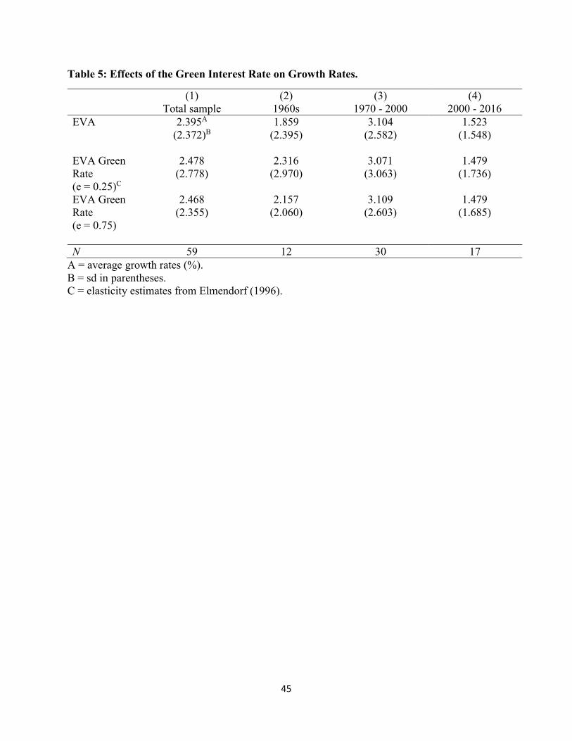
c. Changes in Damages from the Green Interest Rate.

Together with estimates of the elasticity of consumption with respect to changes in interest

rates8, and the green interest rate reported in table 3, the intertemporal reallocation of

consumption and damage induced by the green interest rate is calculated. The details of the

calculation are shown in the appendix. The changes in consumption and damage are used to

compute EVA conditional on consumers facing the green interest rate. The resulting impacts on

EVA growth are reported in table 5. Across the entire 60-year period, the green interest rate

induces a modest 8 basis point increase in growth rates. However, this small boost to growth

masks considerable temporal variability. The largest change to growth rates occurs prior to 1970;

the green interest rate induces a 46 basis point increase to growth. Because the GED was rapidly

changing through the 1950s and 1960s (recall from table 2 that GED grew at nearly 4 percent,

annually before 1970) the reallocation of consumption due to the green interest rate has a large

effect on GED levels and the EVA. Following the 1970 passage of the Clean Air Act, GED

comprise a much smaller share of GDP and the effect of reallocation due to the green rate is

much smaller.

The total reduction in premature mortalities from air pollution exposure due to the green interest

rate ranges between 7,000 and 25,000 as shown in figure A.6. The range of total avoided deaths

stems from the two elasticities used. Early in the sample, deaths rise due to the consumption

reallocation. This occurs because damages increased at an increasing rate. Total avoided deaths

8 Two values (0.25 and 0.75) from Elmendorf (1996) are used.

28

turn negative in 1970. Mortalities from air pollution continue to fall until about 1980. Hence, the

majority of these reductions occurs immediately following passage and prior to full

implementation of the Clean Air Act. While these reductions are a small fraction of total deaths

from pollution, and of the emission changes induced by the Clean Air Act, this new

environmental-macroeconomic policy dimension could have provided an important stopgap prior

to the Clean Air Act.

Importantly, the conceptual model considers two time periods which need not be consecutive or

adjacent. That is, the green interest rate could be computed over longer maturities. Figure A.7

models the case in which the green interest rate is modeled over a five-year maturity. Thus,

consumers face longer consumption-savings tradeoffs than in the two period maturities modeled

in figure A.6. The effect of this longer maturity on avoided mortalities is considerable. Rather

than a range between 7,000 and 25,000 avoided deaths, figure A.7 reveals that the five-year

maturity avoids nearly 60,000 deaths (assuming the 0.25 elasticity). This larger reduction in

PM2.5 deaths occurs because the term that drives the difference between the federal funds rate

and the green interest rate ( ) ( )

( ), is much greater over five-year periods.

d. Variance in Market and Adjusted Consumption.

The top panel of table 6 reports the partial correlation coefficients between GDP and air

pollution, CO2, and combined GED. The 60-year sample is divided into the years prior to the

passage of the CAA, 1970 to 2000, and 2000 to 2016. Column (1) of the top panel indicates that

both combined damage and air pollution damage are negatively correlated with GDP in levels (p

< 0.01). In contrast, CO2 damages are nearly perfectly, positively correlated with GDP (p <

0.01). Columns (2) and (3) highlight the importance of environmental policy. Before passage of

the CAA, air pollution and CO2 damage were positively correlated with GDP (p < 0.01).

29

However, after the CAA became law, air pollution damage became negatively associated with

GDP (p < 0.01), while CO2 remained positively correlated with GDP (p < 0.01). And, after the

year 2000, the sign of the correlations between local air pollution, CO2, and GDP remained as

they were after 1970 (p < 0.01).

The second panel of table 6 explores correlations in growth rates. Across the full sample, GDP

growth was positively correlated with air pollution, and CO2 damage growth (p < 0.01). The key

insight here is that the correlation between GDP growth and air pollution damage growth

weakened after the passage of the CAA both in magnitude of the correlation coefficient and in

statistical significance. In contrast, the correlation between CO2 damage growth and GDP growth

strengthened.

Figure 3 provides an alternative, supporting perspective on these results. In both panels, CO2

moves in lock step with GDP. The left panel shows that both GDP and CO2 damage roughly

triple between 1957 and 2016. The right panel displays the strong positive correlation between

CO2 growth and GDP growth. However, air pollution damage, while rising with GDP through

1970, then fell to 75 percent of its real value in 1957. The right panel of figure 3 shows

consistently negative growth in air pollution damage after 1970, while GDP growth remained

mostly positive. In both panels, drawing on a theme from section IV.b above, the importance of

the business cycle is clear.

The bottom portion of table 6 reports the variances of EVA, GDP, and GED (combined CO2 and

air pollution). In general, EVA levels and growth were more variable than GDP levels and

growth over the 1957 to 2016 period. However, the relative degrees of volatility changed before

and after the passage of the CAA. EVA was less variable than GDP before 1970 (in both levels

and growth). This stems from the strong positive correlation between GDP and GED before

30

1970. In striking contrast, EVA was more variable than GDP between 1970 and 2000. Again, the

top panel of table 6 conveys strong negative correlations between GDP and GED levels from

1970 to 2000. In light of expression (14), the negative correlation boosts the variance of EVA.

Similarly, the positive correlation between GED growth and GDP was substantially weaker after

1970 than before. Thus, all else equal, EVA volatility was enhanced by this effect as shown in

the bottom panel, column (3).

These empirical calculations show that, in levels, pollution damage was positively correlated

with GDP prior to the enactment of the Clean Air Act, and negatively correlated afterwards.

Further, growth rates in pollution damage began strongly, positively correlated and became

weakly correlated after 1970. The effect of these changes in the relationships between damage

and GDP is a reorientation of the variance of EVA and GDP. Prior to the passage of the Clean

Air Act, EVA is less volatile than GDP. However, following passage and enactment, EVA is

more variable both in levels and growth rates.

V. Conclusions.

This paper proposes a novel intersection between environmental policy and two aspects of

macroeconomic policy: volatility in per capita consumption and interest rates. This intersection

fundamentally stems from a redefinition of consumption to include pollution damage that rests

on a firm footing established in the environmental accounting literature (Nordhaus and Tobin,

1973). The paper shows that the covariance between productivity and pollution is the critical

determinant of whether pollution-adjusted consumption is more or less variable than market

consumption. And, the sign of this covariance term depends on whether pollution is regulated

because in an unregulated setting, the covariance term would almost assuredly be positive.

Further, by extending consumption beyond just market-produced goods and services to include

31

pollution damage, the paper develops an expression for natural interest rates that depends on the

trajectory of pollution intensity of output. Economies on a cleaning up path should feature

somewhat higher interest rates (relative to conventionally-defined rates) because future

consumption incurs a smaller pollution penalty. Thus, the higher green interest rate delays

consumption to the less pollution intensive state. In contrast, economies becoming more polluted

should feature lower interest rates. This incentivizes more current consumption in the less

polluted economy.

The empirical portion of the paper shows that the green interest rate exceeds the federal funds

rate by about 50 basis points. However, prior to the passage of the Clean Air Act in 1970, the

green interest rate fell short of the federal funds rate because pollution damages were rising.

Once, the Act was passed, enacted, and implemented, damages from air pollution fell. This

caused the orientation between market rates and the green interest rate to switch, with the green

rate exceeding the federal funds rate in the post-1970 context of falling damage.

The passage of the Act also induced a reversal of the relative magnitudes of volatility in GDP

and adjusted consumption. Prior to the Clean Air Act, the variance in adjusted consumption was

less than that of GDP because positively correlated productivity and pollution shocks dampened

the variance in EVA. After 1970, negatively correlated shocks amplified consumption volatility.

The empirical analysis highlights two sources of environmental damage: CO2 and local air

pollutants. Recent research suggests that damages from these pollutants amount to a considerable

share of GDP (Muller, 2019a; 2019b). The present paper demonstrates that the regulatory status

of the two types of pollution dictates the nature of correlation between damage and productivity

shocks. Unregulated CO2 is positively correlated with GDP. Local air pollutants were regulated

beginning in 1970. Prior to this date damages from these substances covaried positively with

32

GDP. After 1970, the covariance became negative. This result has broad implications for future

research that may seek to incorporate additional pollutants, or sources of environmental goods

and services, into the extended measure of consumption used herein. Namely, unregulated

externalities driven by procyclical emissions will dampen volatility in consumption. Residual

damages from managed emissions will, in contrast, accentuate variability provided regulation is

stringent enough to induce negatively correlated damages and output.

33

References.

1) Abraham, Katherine G., and Christopher Mackie. 2006. “A Framework for Nonmarket

Accounting.” In D.W. Jorgensen, J.S. Landefeld, and W.D. Nordhaus, eds. A New

Architecture for the U.S. National Accounts. NBER Studies in Income and Wealth. Vol.

66, The University of Chicago Press. Chicago, Il, USA.

2) Clay, K., Lewis, J., & Severnini, E. 2016. Canary in a Coal Mine: Infant Mortality, Property

Values, and Tradeoffs Associated with Mid-20th Century Air Pollution (No. w22155).

National Bureau of Economic Research.

3) Costa, D.L., M.E. Kahn. 2004. “Changes in the Value of Life, 1940 – 1980.” Journal of

Risk and Uncertainty. 29(2): 159 – 180.

4) Dockery, Douglas W., C. Arden Pope, Xiping Xu, John D. Spengler, James H. Ware,

Martha E. Fay, Benjamin G. Ferris, Jr., and Frank E. Speizer. “An Association between

Air Pollution and Mortality in Six U.S. Cities.” New England Journal of Medicine.

329:1753-1759.

5) Elmendorf, Douglas, W. 1996. “The Effect of Interest-Rate Changes on Household Saving

and Consumption: A Survey.” Unpublished Working Paper.

6) Fann, Neal, Charles M. Fulcher, Bryan J. Hubbell. 2009. “The influence of location, source

and emission type in estimates of the human health benefits of reducing a ton of air

pollution.” Air Quality Atmosphere and Health. 2:169 – 176.

7) Federal Reserve Economic Data (FRED), 2019a. Nonfarm Business Sector: Hours of All

Persons, Index 2012=100, Quarterly, Seasonally Adjusted. HOANBS.

8) Federal Reserve Economic Data (FRED), 2019b. Effective Federal Funds Rate, Percent,

Monthly, Not Seasonally Adjusted. FEDFUNDS.

9) Goodfriend, Marvin. 2004. “Monetary Policy in the New Neoclassical Synthesis: A

Primer.” Federal Reserve Bank of Richmond. Economic Quarterly. Volume 90/3: 21- 45.

10) Goodfriend, Marvin. 2016. “The Case for Unencumbering Interest Rate Policy at the

Zero Bound.” Designing Resilient Monetary Policy Frameworks for the Future, A

Symposium Sponsored by the Federal Reserve Bank of Kansas City, Jackson Hole,

Wyo., August 25-27, 2016, Federal Reserve Bank of Kansas City, 2016, pp. 127-160.

34

11) Hammitt, J.K., L.A. Robinson. 2011 “The Income Elasticity of the Value per Statistical

Life: Transferring Estimates between High and Low Income Populations.” Journal of

Benefit-Cost Analysis. 2(1): 1 -27.

12) Kaplan, R.S. 2018. “The Neutral Rate of Interest.” Federal Reserve Bank of Dallas.

13) Kleckner, N., and J. Neumann. 1999. Recommended Approach to Adjusting WTP

Estimates to Reflect Changes in Real Income. Memorandum to Jim DeMocker, U.S.

EPA/OPAR. June 3. Available at

http://www.epa.gov/ttn/ecas/regdata/Benefits/background/klecknerandneumann1999.pdf.

14) Krewski D, Jerrett M, Burnett RT, Ma R, Hughes E, Shi, Y, et al. 2009. Extended follow-

up and spatial analysis of the American Cancer Society study linking particulate air

pollution and mortality. HEI Research Report, 140, Health Effects Institute, Boston, MA.

15) Laubach, T. and J.C. Williams, 2003. “Measuring the Natural Rate of Interest.” Review of

Economics and Statistics. 85(4), November, 1063–1070.

16) Laubach, T. and J.C. Williams, 2015. “Measuring the Natural Rate of Interest Redux.”

Federal Reserve Bank of San Francisco Working Paper Series 2015-16.

17) Lave, Lester B., and Eugene Seskin. 1973. “An Analysis of the Association Between U.

S. Mortality and Air Pollution.” Journal of the American Statistical Association, Vol. 68,

No. 342. pp. 284-290.

18) Lepeule J, Laden F, Dockery D, Schwartz J. 2012. “Chronic Exposure to Fine Particles

and Mortality: An Extended Follow-Up of the Harvard Six Cities Study from 1974 to

2009.” Environmental Health Perspectives. 120 (7):965-70.

19) Levy, Jonathan I., Lisa K. Baxter, Joel Schwartz. 2009. “Uncertainty and Variability in

Health-Related Damages from Coal-fired Power Plants in the United States.” Risk

Analysis. DOI: 10.1111/j.1539-6924.2009.01227.

20) Lucas, Robert. 1981. Studies in Business Cycle Theory. Cambridge, MIT Press.

21) Meng, J.; Li, C.; Martin, R. V.; van Donkelaar, A.; Hystad, P.; Brauer, M. 2019. “Estimated

Long-term (1981-2016) Concentrations of Ambient Fine Particulate Matter across North

America from Chemical Transport Modeling, Satellite Remote Sensing and Ground-based

Measurements.” Environmental Science and Technology. DOI: 10.1021/acs.est.8b06875

35

22) Muller, Nicholas Z., 2014. "Boosting GDP growth by accounting for the environment:

Including air pollution and greenhouse gas damages increases estimated U.S. growth."

Science. August 22nd, 2014, Vol. 345 no. 6199 pp. 873-874:

23) Muller, Nicholas Z., 2019a. "Long-Run Environmental Accounting in the United States

Economy.” National Bureau of Economic Research, WP #25910.

24) Muller, Nicholas Z., 2019b. "The Derivation of Discount Rates with an Augmented

Measure of Income.” Journal of Environmental Economics and Management:

https://doi.org/10.1016/j.jeem.2019.02.007.

25) Muller Nicholas Z., Robert O. Mendelsohn, 2009. Efficient Pollution Regulation:

Getting the Prices Right. American Economic Review. 99(5): 1714 – 1739.

26) Muller, Nicholas Z., Robert O. Mendelsohn, and William D. Nordhaus, 2011.

Environmental Accounting for Pollution in the U.S. Economy. American Economic

Review. 101(5): 1649 – 1675.

27) National Academy of Sciences, National Research Council. 1999. Nature’s Numbers:

expanding the U.S. national economic accounts to include the environment. W.D.

Nordhaus and E.C. Kokkelenberg, eds. National Academy Press, Washington, D.C.,

USA.

28) Nordhaus, William D., J. Tobin. 1973. “Is Growth Obsolete?“ in Economic Research:

Retrospect and Prospect-Economic Growth, 50th Anniversary Colloquium V, New York:

Columbia University Press for National Bureau of Economic Research.

29) Nordhaus, William D. 2006. “Principles of National Accounting for Non-Market

Accounts.” In D.W. Jorgensen, J.S. Landefeld, and W.D. Nordhaus, eds. A New

Architecture for the U.S. National Accounts. NBER Studies in Income and Wealth. Vol.

66, The University of Chicago Press. Chicago, Il, USA.

30) United States Bureau of Economic Analysis. 2019:

http://www.bea.gov/iTable/index_nipa.cfm.

31) United States Department of Energy (USDOE), 2011.

https://www.eia.gov/totalenergy/data/annual/pdf/sec11.pdf

32) United States Department of Energy (USDOE), 2019. Table 12.1 Carbon Dioxide

Emissions From Energy Consumption by Source.

36

33) United States Environmental Protection Agency. 1999. The Benefits and Costs of the Clean

Air Act: 1990--2010. EPA Report to Congress. EPA 410-R-99-001, Office of Air and

Radiation, Office of Policy, Washington, D.C.

34) United States Environmental Protection Agency. 2010. The Benefits and Costs of the Clean

Air Act: 1990--2020. Final Report. Office of Air and Radiation, Office of Policy,

Washington, D.C.

35) United States Interagency Working Group on Social Cost of Carbon (USFWG). 2016.

Technical Support Document: Technical Update of the Social Cost of Carbon for

Regulatory Impact Analysis Under Executive Order 12866.

https://www.epa.gov/sites/production/files/2016-

12/documents/sc_co2_tsd_august_2016.pdf

37

Figure 1: Inter-temporal Consumption Choices with Green Interest Rate.

38

Figure 2: GDP, Pollution Damage, and EVA.

Vertical lines demarcate NBER recessions.

Solid = GDP; Dash = EVA; Dash-dot = GED.

EVA = GDP – GED

39

Figure 3: GDP, Air Pollution and CO2 Damage.

Solid = Real GDP

Dash = Real CO2 GED

Dash-dot = Real air pollution GED

Vertical lines demarcate NBER recessions.

40

Figure 4: Federal Funds Rate and Green Interest Rates.

Left panel LOWESS smooth: Solid = Federal Funds Rate; Dash = Green Interest Rate.

Right panel: Green Interest Rate – Federal Funds Rate.

41

Tables.

Table 1: Output and Damage per Capita.

(1) (2) (3) (4) (5) (6) (7) Total sample 1960s 1970s 1980s 1990s 2000s 2010s GDP 35456.87A 20379.25 26983.46 32830.41 40247.88 49315.88 52672.27 (11844.9) (2538.2) (1924.6) (2837.3) (2790.2) (2101.2) (1715.5) EVA 28661.08 13546.24 18053.70 25259.12 33873.43 43700.98 47813.06 (12760.0) (1064.1) (2300.0) (3084.0) (3000.7) (2279.2) (1803.8) Air 6795.79 6833.00 8929.76 7571.29 6374.45 5614.90 4859.21 + Climate (1467.4) (1509.0) (469.1) (446.5) (297.0) (410.3) (117.2) Air 6347.24 6588.28 8555.26 7155.21 5856.45 4994.69 4224.37 (1545.5) (1473.2) (489.3) (454.8) (326.5) (411.4) (128.4) Climate 448.55 244.72 374.50 416.09 517.99 620.21 634.84 (145.1) (36.51) (27.49) (30.58) (36.52) (23.02) (21.53) N 60 13 10 10 10 10 7

A = ($2012)

Standard deviations in parenthesis.

42

Table 2: Growth Rates of Per Capita Output and Damage.

(1) (2) (3) (4) (5) (6) (7) Total sample 1960s 1970s 1980s 1990s 2000s 2010s GDP 1.90A 2.56 2.07 2.10 1.97 0.93 1.51 (2.105) (2.524) (2.421) (2.506) (1.550) (2.048) (0.575) EVA 2.40 1.86 3.51 3.15 2.65 1.43 1.66 (2.372) (2.395) (3.309) (2.732) (1.628) (1.968) (0.733) Air + Climate -0.35 3.89 -0.95 -1.37 -1.49 -2.87 -0.08 (5.065) (5.743) (3.467) (4.577) (2.832) (6.498) (3.426) Air -0.55 3.90 -1.12 -1.53 -1.78 -3.28 -0.30 (5.338) (5.914) (3.485) (4.721) (3.040) (7.084) (3.709) Climate 1.98 3.36 3.03 1.25 1.92 0.48 1.36 (2.829) (1.710) (3.293) (3.564) (1.256) (3.111) (3.011) N 59 12 10 10 10 10 7

A = all values are average growth in (%)

Standard deviations in parenthesis.

43

Table 3: Comparison of Federal Funds Rate and Green Interest Rate.

(1) (2) (3) (4) (5) (6) (7) Total sample 1957 –

1970 1970s 1980s 1990s 2000s 2010s

Federal Funds 5.04 3.83 7.10 9.97 5.15 2.96 0.16 (3.558) (1.730) (2.428) (3.152) (1.403) (2.012) (0.106) Green Rate 5.60 3.19 8.62 11.06 5.84 3.45 0.32 (4.252) (2.711) (3.143) (3.601) (1.589) (2.039) (0.429) Green Rate- 0.52*** -0.72 1.52** 1.10** 0.70*** 0.50** 0.16 Federal Funds

(1.495) (2.041) (1.738) (1.321) (0.534) (0.699) (0.366)

N 60 13 10 10 10 10 7 mean coefficients; sd in parentheses * p < 0.05, ** p < 0.01, *** p < 0.001 for t-test of rate difference H0 = 0.

44

Table 4: Comparison of Federal Funds Rate and Green Interest Rate Across the Business Cycle. (1) (2) (3) (4) (5) (6) (7) Total

sample Recession Expansion Recession

Pre-1970 Expansion Pre-1970

Recession Post-1970

Expansion Post-1970

Federal 5.04 6.50 4.42 3.61 3.97 7.62 4.52 Funds (3.558) (4.493) (2.917) (2.665) (1.007) (4.626) (3.209) Green 5.60 7.44 4.85 4.00 2.75 8.49 5.35 Rate (4.254) (5.150) (3.645) (3.456) (2.438) (5.219) (3.731) Green 0.52*** 0.73*** 0.43** 0.27 -1.22* 0.88** 0.82*** Rate - Fed. Funds

(1.495) (1.651) (1.439) (1.262) (2.242) (1.773) (0.830)

N 60 18 42 5 8 13 34 mean coefficients; sd in parentheses * p < 0.05, ** p < 0.01, *** p < 0.001 for t-test of rate difference H0 = 0.

45

Table 5: Effects of the Green Interest Rate on Growth Rates.

(1) (2) (3) (4) Total sample 1960s 1970 - 2000 2000 - 2016 EVA 2.395A 1.859 3.104 1.523 (2.372)B (2.395) (2.582) (1.548) EVA Green 2.478 2.316 3.071 1.479 Rate (e = 0.25)C

(2.778) (2.970) (3.063) (1.736)

EVA Green 2.468 2.157 3.109 1.479 Rate (e = 0.75)

(2.355) (2.060) (2.603) (1.685)

N 59 12 30 17

A = average growth rates (%). B = sd in parentheses. C = elasticity estimates from Elmendorf (1996).

46

Table 6. Variance and Correlations between per Capita GDP and Pollution Damage.

(1) (2) (3) (4) Correlation Levels

Total sample 1960s 1970 - 2000 2000 - 2016

Air + Climate -0.586***A 0.990*** -0.936*** -0.696** Air -0.649*** 0.990*** -0.944*** -0.724** Climate 0.990*** 0.994*** 0.980*** 0.831***

Growth

Air + Climate 0.583*** 0.753** 0.516** 0.570* Air 0.567*** 0.753** 0.498** 0.544* Climate 0.661*** 0.593* 0.642*** 0.784***

Variance Levels

GDP 1.40B 6.44 36.5 6.49 EVA 1.63 1.13 50.7 8.49 Air + Climate 2.15 2.28 1.29 2.47

Growth

GDP 4.43C 6.37 4.52 2.57 EVA 5.63 5.74 6.67 2.40 Air + Climate 25.66 32.99 12.77 30.16 N 59 12 30 17

* p < 0.05, ** p < 0.01, *** p < 0.001 A = pairwise Pearson’s correlation coefficient between each listed variable and GDP growth. B = ($2012) millions. C = growth rates (%).

47

Appendix

The supplementary appendix contains three sections. It begins with a discussion of the methods

and results from a set of calculations that demonstrate how intertemporal consumption and

damages would change if the green interest rate faced households, rather than actual market rates

are approximated by the 10-year Treasury bond. The second and third subsections include

additional figures and tables that support the main text.

I. Substitution between environmental damage and consumption.

An important issue in the context of the present paper is substitution between consumption of

market goods and environmental quality, or damage. The simple, univariate power utility

function employed in section II. of the main body of the paper is easily augmented to include

environmental quality in a separable fashion. For example, Hoel and Sterner (2007) propose a

utility function of the form:

𝑈 (𝑐 , 𝑒 ) = (1 − 𝜃)𝑐 + (𝜃) 𝑐 (𝛼 − 𝛽 𝛾 ) 𝑒

( )

a.1

where: 𝜎 = constant elasticity of substitution between environmental quality (et) and market goods (ct). 𝜃 = scaling parameter proportional to consumption shares of environmental quality (et) and market goods (ct). One central question is whether, conditional on the form shown in (a.1), the first order condition

with respect to consumption of market goods is affected. Recall from section II., that this first

order condition plays a key role in the conceptual analysis which solves for the green interest

rate.

To explore this, the marginal utility from market consumption is derived for t = 1 and t = 2. Here

the assumption of log utility is maintained for simplicity. This assumption yields (a.2).

48

𝑈 (𝑐 , 𝑒 ) = 𝑙𝑛 (1 − 𝜃)𝑐 + (𝜃) 𝑐 (𝛼 − 𝛽 𝛾 ) 𝑒 (a.2)

Setting marginal utilities from consumption of market goods in periods 1 and 2 equal and

rearranging yields (a.3) which is identical to (2).

= (a.3)

Thus, with power utility and with 𝜂 = 1, the key form used to derive interest rates is unaffected

by allowing arbitrary substitution between market goods and environmental quality in the

representative consumer’s utility function.

It is important to note that environmental quality does not enter into the utility function as

employed into the main body of the paper. Rather, environmental pollution damage is, in effect,

deducted from potential income. This treatment reflects guidance from the environmental

accounting literature (Nordhaus, 2006; Abraham and Mackie, 2006). This tack does imply

substitution between damage and consumption (through the adjustment of potential income).

This assumption that damages are deducted from potential income manifests through the

intercepts of the intertemporal budget constraint as shown in figure 1.

II. Damage change from green interest rates.

In order to (empirically) estimate the effect that implementation of the green interest rate would

have on consumption and damages the following approach is used. First, it is assumed that

consumers face a series of two period consumption-savings decisions in accord with the structure

of the theoretical model used in the main body of the paper. Thus, in period (t), households

decide how much to consume and save. In period (t+k), households face a new interest rate and

49

they repeat this process. The resulting change in consumption is translated to damages using the

empirically estimated damage intensity of output (GED/GDP) in periods (t) and (t+k). The sum

of damages over each pair of periods is computed from 1957 to 2016. These damage estimates

are then deducted from the observed GED, matched to each pair of years. These calculations are

shown in (a.4).

∆𝐺𝐸𝐷 = (∆𝑟 𝜀 𝐺𝐸𝐷 − ∆𝑟 𝜀 𝐺𝐸𝐷 + (∆𝑟 𝜀 𝐺𝐸𝐷 ) (a.4)

In (a.4), 𝜀 denotes consumers’ elasticity of savings with respect to the interest rate, and (∆𝑟) is

the difference between market and the green interest rate (expression 6). Estimates of 𝜀 , 0.25

and 0.75, are drawn from the literature (Elmendorf, 1996).

In addition to modeling year-over-year consumption/savings tradeoffs induced by the green

interest rate, the empirical analysis explores longer maturities. The basic structure of the

simulation is identical to that described above except that k = 5 in (a.4) rather than k = 1. Figure

A.7 shows that the avoided deaths due to the longer term (five-year) green interest rate are much

higher than under the one-year maturity. Specifically, a total of 60,000 avoided mortalities

accrue if households faced the 5-year green interest rate as opposed to just under 8,000 with the

one-year rate.

50

Supplementary Figures.

Figure A.1: Annual Average PM2.5 Concentrations: Satellite-Monitor Comparison.

Squares = USEPA AQS Monitor Data, Circles = PM2.5 Data from Meng et al., (2019).

Source: Muller (2019b).

51

Figure A.2: TSP and PM2.5 National Average Concentrations.

Dash = PM2.5 (95% Confidence intervals on predicted values prior to 1980); Solid = TSP Vertical lines demarcate NBER recessions. Source: Muller (2019b).

52

Figure A.3: VSL under various assumptions.

Source: Muller (2019a).

Solid: default VSL used in the present analysis.

Dash: VSL-income elasticity = 0.4

Dash-dot: VSL-income elasticity = 1.0

53

Figure A.4: U.S. Economy CO2 Emissions and Social Cost of Carbon Estimates.

Solid line = CO2 emission estimates.

Squares = SCC.

54

Figure A.5: Real, Per Capita Air Pollution and CO2 GED.

Solid = air pollution; Dash = CO2.

55

Figure A.6: Change in PM2.5 Deaths due to Households Facing Green Interest Rate.

Solid = assumes elasticity of savings of 0.25.

Dash = assumes elasticity of savings of 0.75.

56

Figure A.7: Change in GED due to Households Facing Green Interest Rate with 5-Year Maturity.

Solid = one year maturity.

Dash = five year maturity.

57

Supplementary Tables.

Table A1: Summary Statistics by Decade.

(1) (2) (3) (4) (5) (6) (7) Total

sample 1960s 1970s 1980s 1990s 2000s 2010s

Abatement 1.0001A 1.0000 1.0005 0.9998 0.9998 1.0002 1.0000 (0.00071) (0) (0.0016) (0.00028) (0.00002) (0.0002) (0.0001) Green 0.0052B -0.0074 0.0146 0.0107 0.0068 0.0050 0.0016 Coefficient (0.0146) (0.0203) (0.0171) (0.0132) (0.00517) (0.00684) (0.00357) GED/GDP 0.2088D 0.3235 0.3194 0.2200 0.1465 0.1016 0.0803 (0.101) (0.0312) (0.0384) (0.0294) (0.0169) (0.0110) (0.00476) N 59 12 10 10 10 10 7

All statistics in table A1 are year over year ratios.

A = fraction of GDP spent on abatement of air pollution (USEPA, 2011).

B = ( ) ( )

( )

C = Hours of all persons worked in non-farm business sector (FRED, 2019).

58

Table A2: Summary Statistics and the Business Cycle.

(1) (2) (3) (4) (5) Total sample Recession Not Recession Energy Crisis Great Recession Abatement 1.0001A 1.0004 0.9999 1.0027 1.0003 (0.000711) (0.00125) (0.000199) (0.00326) (0.000130) Green 0.0052B 0.0089 0.0036 0.0223 0.0049 Coefficient (0.0146) (0.0169) (0.0134) (0.00148) (0.00719) GED/GDP 0.2088D 0.2420 0.1942 0.3303 0.0903 (0.101) (0.0967) (0.0999) (0.0106) (0.00776) N 59 18 41 2 3

All statistics in table A2 are year over year ratios.

A = fraction of GDP spent on abatement of air pollution (USEPA, 2011).

B = ( ) ( )

( )

C = Hours of all persons worked in non-farm business sector (FRED, 2019).

59

Table A3: Growth Rates and the Business Cycle.

(1) (2) (3) (4) (5) (6) (7) Total

sample Recession Expansion Recession

Pre-1970 Expansion Pre-1970

Recession Post-1970

Expansion Post-1970

GDP 1.90 -0.35 2.81 0.06 3.81 -0.47 2.57 (2.105) (2.134) (1.249) (2.732) (1.209) (2.034) (1.153) EVA 2.39 0.36 3.21 0.36 2.65 0.37 3.34 (2.346) (2.497) (1.723) (2.133) (2.189) (2.678) (1.606) GED -0.55 -3.20 0.53 -0.49 6.10 -4.03 -0.79 (5.338) (5.742) (4.832) (5.266) (5.153) (5.815) (3.751) N 59 17 42 4 8 13 34