multi-agent simulation-based virtual test bed ecosystem
TRANSCRIPT

New York University
Rutgers University
University of Washington
The University of Texas at El Paso
City College of New York A USDOT University Transportation Center
Multi-agent Simulation-based
Virtual Test Bed Ecosystem:
MATSim-NYC
May 2020

Multi-Agent Simulation-Based Virtual Testbed In Nyc ii
Multi-agent Simulation-based Virtual Test Bed Ecosystem: MATSim-NYC
Joseph Y.J. Chow New York University
0000-0002-6471-3419 Kaan Ozbay
New York University 0000-0001-7909-6532
Yueshuai He
New York University 0000-0002-5794-7751
Jinkai Zhou
New York University 0000-0002-1563-1329
Ziyi Ma New York University
Mina Lee
New York University 0000-0002-4945-4738
Ding Wang
New York University 0000-0002-2398-1409
Di Sha
New York University
C2SMART Center is a USDOT Tier 1 University Transportation Center taking on some of today’s most pressing urban mobility challenges. Some of the areas C2SMART focuses on include:
Urban Mobility and Connected Citizens
Urban Analytics for Smart Cities
Resilient, Smart, & Secure Infrastructure
Disruptive Technologies and their impacts on transportation systems. Our aim is to develop innovative solutions to accelerate technology transfer from the research phase to the real world.
Unconventional Big Data Applications from field tests and non-traditional sensing technologies for decision-makers to address a wide range of urban mobility problems with the best information available.
Impactful Engagement overcoming institutional barriers to innovation to hear and meet the needs of city and state stakeholders, including government agencies, policy makers, the private sector, non-profit organizations, and entrepreneurs.
Forward-thinking Training and Development dedicated to training the workforce of tomorrow to deal with new mobility problems in ways that are not covered in existing transportation curricula.
Led by New York University’s Tandon School of Engineering, C2SMART is a consortium of leading research universities, including Rutgers University, University of Washington, the University of Texas at El Paso, and The City College of NY.
Visit c2smart.engineering.nyu.edu to learn more

Multi-Agent Simulation-Based Virtual Testbed In Nyc iii
Disclaimer
The contents of this report reflect the views of the authors, who are responsible for the facts and the
accuracy of the information presented herein. This document is disseminated in the interest of
information exchange. The report is funded, partially or entirely, by a grant from the U.S. Department of
Transportation’s University Transportation Centers Program. However, the U.S. Government assumes no
liability for the contents or use thereof.
Acknowledgements
The development of simulation test bed in MATSim involved collaboration with Dr. Balac Milos from ETH
Zurich and Joon Park from New York City Department of Transportation. Dr. Abdullah Kurkcu and Yubin
Shen supported the data sharing and management. PhD candidate Qi Liu assisted the calibration of
transit vehicle capacity and PhD candidate Haoran Su helped with the preparation of transit schedules.

Multi-Agent Simulation-Based Virtual Testbed In Nyc iv
Executive Summary
To grapple with emerging technologies, city agencies need to evaluate operational scenarios imposed by
private sector (e.g. what is the impact of e-hail ride-sourcing on traffic congestion?) or when considering
what-if scenarios related to new operating policies. This is especially important because technologies
companies developing public products need to gain approval from public agencies before they can
deploy in that region. As such, public agencies need to evaluate the product’s impact on the community.
Transportation products like policies and operating technologies face different challenges than
conventional technologies because of their public nature. Transportation technologies deployed to the
field can be both financially and socially costly, as unproven technologies may end up costing lives if
something goes wrong. Furthermore, even a successful deployment in one city may not be indicative
that the same technology can work well in another city because each city is a different market.
Prototyping serves to verify that a technology works, but it does not consider how the technology may
impact a community given the behavior of its population. This gap in the innovation process for
transportation technologies suggests a need for a deployment testing framework that falls between
prototyping and field piloting. Existing tools like NYBPM are designed more for long term capital
planning than for quick response evaluation of operating policies introduced by emerging transportation
technologies, which are often dynamic and impact travelers’ travel preferences throughout the day.
Congestion pricing, algorithms for microtransit or bikeshare rebalancing, electric vehicle fleets with
dynamic fast charging activities all impact travelers’ choices throughout the day, which in turn impact
the dynamics of traffic congestion throughout the day. These interactions are currently not addressed
by any existing tools in NYC, nor in most cities around the world.
One of the missions of C2SMART is to help cities around the country better understand the
transferability of transportation technologies. For this purpose, we initiated two yearlong projects from
2018 – 2020 to initiate a new virtual test bed ecosystem:
• 2018 – 2019: Phase I: Open Source Multi-Agent Virtual Simulation Testbed
• 2019 – 2020: Phase II: Development and Tech Transfer of Multi-Agent Simulation Testbed
This report covers the findings of both years’ projects. The objective of these two projects is to develop
an initial architecture and virtual test bed that can be replicated in future projects to other cities in the
C2SMART consortium and partners. The vision is for a “Network of Living Labs”, which is tentatively
dubbed as C2SMART’s “NOLL-Edge” system. Its goal is to be used by city agencies to evaluate emerging
technologies and operating policies using a consistent platform so that their effects can be quantified. In
the long term, cities may opt to use this test bed as a means of certification for policies and technologies
(e.g. NOLL-Edge-certified that policy A can achieve X% welfare improvement in NYC or reduce
congestion by Y% for population segments 1, 2, 3, etc.). The test bed system is integrated within an
Urban Data Observatory. Users of the virtual test bed are divided into 3 groups: (a) agencies that want

Multi-Agent Simulation-Based Virtual Testbed In Nyc v
to evaluate a scenario; (b) technology companies that want to submit their technologies for deployment
testing; (c) research partners who want to conduct research using data from the system. Users need to
be able to query data, define scenarios with C2SMART for which comparisons to baseline scenario are
made, submit extensions that capture new technologies to use in a scenario, or develop a new model
that better fits the needs of the scenario to be evaluated.
We developed an initial test bed for NYC using MATSim, a Multi-Agent Transportation Simulation.
MATSim models transportation networks using a mesoscopic simulation based on cellular automata. It is
open source and many extensions have been quickly developed for it to handle a wide assortment of
policy needs: autonomous vehicles, emissions modeling, parking, freight, electric vehicles, bikeshare,
etc. MATSim makes use of a synthetic population which is useful for modeling heterogeneous
population segments. It incorporates a day-to-day adjustment process that can reflect learning from the
population to achieve a social equilibrium under each technology scenario.
Based on this overarching goal, we set out on these two projects with the following set of objectives:
• Create an underlying synthetic population for NYC for a recent base year (2016) that includes
key emerging modes like Citi Bike and for-hire vehicles (FHVs) like Uber/Lyft/Via
• Construct, calibrate, and validate a MATSim model of NYC using the synthetic population
• Use the synthetic population and MATSim models to evaluate a set of scenarios for which
existing tools are not equipped:
o The now-defunct plan to establish an Amazon headquarters in Long Island City and the
impact resulting from trips taken by professional service employees to that area
o Citi Bike expansion plan and the resulting effect on travelers, which is not currently
modeled as a mode in any existing travel demand tool for NYC
o Congestion pricing for Manhattan, and its impact on traffic propagation into and out of
Manhattan by time of day
o Brooklyn-Queens Connector (BQX), a proposed streetcar service for which there is no
broad consideration of demand for its service at a citywide level.
• Exploration of other features of MATSim:
o Mobility-on-demand-based autonomous vehicle fleets
o Bike-share
o Multimodal travel
o More realistic traffic flow modeling on the links.
We used the PopGen 2.0 (MARG,2016) to generate the representative synthetic population while
controlling and matching both household-level and person-level attributes. We generated a population
of 8.24 million people for the base year of 2016, compared to a total true population of 8.34 million
people. There was an average of 4% difference between the synthetic population and the Longitudinal
Employer-Household Dynamics 2016 data. Travel agendas were replicated from the 2010/2011 Regional

Multi-Agent Simulation-Based Virtual Testbed In Nyc vi
Household Travel Survey, minus the mode for each trip. Over 30 million trips were synthesized. Modes
were synthesized using a mode choice model.
A tour-based nested logit model was developed and calibrated using the 2010/2011 RHTS for driving,
walking, carpool, public transit (both subway and bus), taxi, and bike. For-hire vehicles (e.g. e-hail,
ridesourcing) and Citi Bike modes were estimated by perturbing the existing model with new modes to
fit count data in 2016 using least squares. An additional smartphone ownership choice model was
estimated to use as an attribute or alternative availability indicator. The model was estimated for two
population segments: people living in Manhattan and those living outside Manhattan. The value of time
for the Manhattan segment was estimated to be $29/h. The model was validated against the 2017
Citywide Mobility Survey from the New York City Department of Transportation (NYC DOT), and found to
fit well.
The completed synthetic population was then fed into MATSim simulation along with data for the road
network from OpenStreetMap, transit schedule from GTFS, and other simulation-level configuration
parameters. Gateway trips were added to account for origins outside of NYC entering through the city,
which account for 1.18M additional population and 3.04M trips. The nested logit model parameters
were converted to equivalent multinomial logit model parameters to fit MATSim’s score function
framework. The road network was calibrated further by speed and capacity, differentiated by time of
day as well as by arterial or freeway. The speeds were initially calibrated against INRIX data while the
capacities were calibrated against the hourly traffic counts of 19 bridges and tunnels around the city.
The resulting model, called MATSim-NYC, had a relative difference on average of 7.2% for the freeways
and 17.1% for the arterials. The simulated screenlines along the bridges and tunnels had an average
relative difference of 25.9% for the Hudson screenline and 2.6% for the East River screenline, with an
overall average relative difference over different time periods of 10.3%. Validation of MATSim-NYC was
conducted using transit ridership across ten of the highest volume ridership and hourly volumes of 15
major locations in NYC. The transit stations show a difference in total daily ridership of 8% while the
median difference for the traffic volumes is 29%.
The calibrated synthetic population and MATSim-NYC model were then applied to create a baseline
scenario from which we analyzed four different scenarios. The first two scenarios are analyzed using the
synthetic population. Scenario 1 looked at building the office space for the Amazon HQ in Long Island
City as originally planned, showing that it would increase morning peak hour trips from 5000 to 8000
while expanding taxi and FHV demand to/from that location by more than four times. Scenario 2 studies
the Citi Bike expansion which predicts the number of daily trips would increase from 47K daily trips to
91K daily trips.
The latter two scenarios are analyzed using MATSim-NYC. Scenario 3 is the congestion pricing plan for
NYC. A $9.18 peak period pricing plan analyzed by RPA is also looked at. Our model predicts twice the

Multi-Agent Simulation-Based Virtual Testbed In Nyc vii
number of cars shifted away (127,000) than RPA (59,000); most of which are absorbed by transit.
Revenues are consistent. In addition, MATSim-NYC allows us to measure the impact on consumer
surplus, suggesting benefits for Manhattanites that are on average 54% higher than for non-
Manhattanites. This warrants more careful redistribution of the pricing revenue toward outer boroughs
transit services. We can also see to which modes the trips shift: 15% of car trips shift to transit and 10%
shift to FHV and taxi. Scenario 4 looks at the Brooklyn-Queens Connector (BQX) and predicts a higher
daily ridership (112K) than the original BQX study (50,000). We also predict a peak load during morning
peak hours of 1400 passengers/hour along with a prediction of 16% of BQX riders shifting from car
mode (18K cars).
A summary of other extensions are also provided: we developed more realistic traffic flow models
within the simulation; we investigated the use of an autonomous mobility-on-demand (AMoD)
extension for MATSim-NYC; we reviewed tools available for handling multimodal routing and bike-share
in MATSim; and we planned out next steps for integrating the test bed in the urban data observatory.
The projects have resulted in presentations given at University of Maryland, ETH Zurich, and ICTPA, as
well as a webinar covering application to congestion pricing and COVID-19. Four papers were prepared
directly from the tool development; several other papers were also prepared in conjunction while
studying multimodal transport and emerging technologies (12 in total). The work has supported two
other projects at C2SMART, supported several PhD students for portions of their dissertations, several
MS theses, a Center for Urban Science and Progress (CUSP) capstone, the The NYU Tandon School of
Engineering's Applied Research Innovations in Science and Engineering (ARISE) program, graduate and
undergraduate courses by Professor Chow, the NYU Tandon Research Expo presented to the public, and
integrated into courses and training for NYCDOT and ITS-NY members.

Multi-Agent Simulation-Based Virtual Testbed In Nyc viii
Table of Contents
Multi-agent Simulation-based Virtual Test Bed Ecosystem: MATSim-NYC ..................................... i
Executive Summary ............................................................................................................................ iv Table of Contents............................................................................................................................... viii List of Figures ...................................................................................................................................... ix List of Tables ........................................................................................................................................ x Section 1: Introduction ........................................................................................................................ 1
Subsection 1.1: Background ............................................................................................................. 1 Subsection 1.2: Research Objectives ............................................................................................... 4 Subsection 1.3: Organization of Report ........................................................................................... 7
Section 2: Overview of agent-based simulations and MATSim ............................................................ 8 Subsection 2.1: Agent-Based Modeling and Simulation .................................................................. 8 Subsection 2.2: MATSim Overview .................................................................................................. 9
Section 3: Synthetic Population ......................................................................................................... 11 Subsection 3.1: Population Synthesis ............................................................................................ 11 Subsection 3.2: Agenda Assignment .............................................................................................. 13 Subsection 3.3: Travel Mode Determination ................................................................................. 14
Section 4: Baseline Model Calibration ............................................................................................... 24 Subsection 4.1: Data Preparation .................................................................................................. 25 Subsection 4.2: Network Calibration ............................................................................................. 30 Subsection 4.3: Calibration Results ................................................................................................ 39 Subsection 4.4: Validation ............................................................................................................. 41
Section 5: Scenario Analyses .............................................................................................................. 44 Subsection 5.1: Scenario One ........................................................................................................ 45 Subsection 5.2: Scenario Two ........................................................................................................ 49 Subsection 5.3: Scenario Three ...................................................................................................... 53 Subsection 5.4: Scenario Four ........................................................................................................ 58
Section 6: Further Extension .............................................................................................................. 61 Subsection 6.1: MATSim Traffic Flow Model Improvement .......................................................... 61 Subsection 6.2: Autonomous Vehicle Fleet ................................................................................... 64 Subsection 6.3: Multimodal Router for MATSim ........................................................................... 69 Subsection 6.4: Bike-sharing Extension ......................................................................................... 72 Subsection 6.5: Urban Data Observatory ...................................................................................... 73
Section 7: Technology Transfer, Dissemination, and Broader Impacts .............................................. 73 Subsection 7.1: Technology Transfer ............................................................................................. 73 Subsection 7.2: Dissemination ....................................................................................................... 74 Subsection 7.3: Broader Impacts ................................................................................................... 76
References ......................................................................................................................................... 77

Multi-Agent Simulation-Based Virtual Testbed In Nyc ix
List of Figures
Figure 1. Spectrum of modes available in a MaaS paradigm (Wong et al., 2020).......................... 1
Figure 2. Selected transit partnerships, several of which are from the MOD Sandbox program
(GAO, 2018) ............................................................................................................................... 2
Figure 3. Illustration of unique aspects of innovation process for transportation technologies .... 3
Figure 4. Conceptual use case diagram of NOLL-Edge system ..................................................... 4
Figure 5. Illustrative screenshot of the MATSim interface ........................................................... 5
Figure 6. Illustrative screenshot of OD data query tool (NTA mode) ............................................ 6
Figure 7. Framework for day-to-day adjustment processes for evaluating market equilibrium of
dynamic transportation systems with user and operating learning (Djavadian and Chow, 2017b) 8
Figure 8. Framework of simulation in MATSim (Horni et al., 2016) ............................................. 11
Figure 9. Comparison of the synthesized and LEHD distributions of the population employment
industry ..................................................................................................................................... 13
Figure 10. Illustration of three tours from an individual: two home-based tours (H-A1-A2-H, H-
A4-H), one non-home-based subtour (A1-A3-A1) ....................................................................... 15
Figure 11. Structure of nested logit model ................................................................................. 15
Figure 12. Aggregated mode share of 2011 RHTS, synthetic population and 2017 CMS .............. 24
Figure 13. Road network from OSM data ................................................................................... 25
Figure 14. Modal network of NYC .............................................................................................. 26
Figure 15. Gateway locations around the city ............................................................................ 27
Figure 16. FDs of MATSim queue-based model (a) Flow vs Density and (b) Speed vs Density ...... 31
Figure 17. The framework of calibration process ........................................................................ 32
Figure 18. Select facilities for link capacity calibration and East River screenline ........................ 34
Figure 19. Distribution of average hourly speed at 12 AM from INRIX data ................................ 34
Figure 20. Comparison of INRIX speed (observed) and simulated speed ..................................... 40
Figure 21. Average simulated and real volume distribution of East River screenline across all time
periods ...................................................................................................................................... 40
Figure 22. Subway locations for validation ................................................................................. 42
Figure 23. Distribution of volume count facilities ....................................................................... 44
Figure 24. Original planned site of Amazon’s NYC Headquarters (LIC Development MOU, 2018) 45
Figure 25. Process flow of experimental design.......................................................................... 46
Figure 26. Spatial distribution of home locations for workers in TAZ 362 (a) in 2016, and (b) in
2028 with Amazon HQ relocation .............................................................................................. 47

Multi-Agent Simulation-Based Virtual Testbed In Nyc x
Figure 27. Time-of-day distribution of inbound and outbound trips at TAZ 362 in 2028 (a) without
Amazon and (b) with Amazon .................................................................................................... 49
Figure 28. Planned Citi Bike service area expansion (Citi Bike, 2019) .......................................... 50
Figure 29. Distribution of synthetic daily Citi Bike trip densities per origin zone under (a) original
service area, (b) Citi Bike’s expansion plan, and (c) the whole city as the service area ................ 52
Figure 30. Charging area in Manhattan ...................................................................................... 53
Figure 31. Daily trip shifts after charging congestion price for charging-related segment ........... 55
Figure 33. Average hourly volume distribution (a) before congestion pricing and (b) under
Schema 2 .................................................................................................................................. 58
Figure 34. Plan of the Brooklyn Queens Connector (BQX, 2019) ................................................. 59
Figure 35. Simulated volume and expected volume across all stations of BQX ............................ 60
Figure 36. Simulated north-bound load profile in AM peak ........................................................ 60
Figure 37. Mode shift of BQX riders ........................................................................................... 61
Figure 38. Overview of the AMoD simulation process ................................................................ 65
Figure 39. AMoD scenario visualization ...................................................................................... 66
Figure 40. Distribution of request per total travel time .............................................................. 67
Figure 41. Distribution of requests served by autonomous taxi .................................................. 67
Figure 42. Distribution of request per drive time ....................................................................... 68
Figure 43. Distribution of requests per wait time ....................................................................... 68
Figure 44. User interface of Open Trip Planner .......................................................................... 70
Figure 45. A Sample Query of Open Trip Planner ....................................................................... 71
List of Tables
Table 1. Sensitivity tests of stability of MATSim predicted trips per mode over four runs ............ 9
Table 2. Attributes available from ACS, LEHD and SED data ........................................................ 12
Table 3. Validation results of the synthetic population comparing with SED data by zone .......... 13
Table 4. Estimation results of nested logit model for both segments .......................................... 20
Table 5. Results of coefficients of Smart Phone ownership model .............................................. 21
Table 6. Estimated parameters and confidence intervals for FHV and Citi Bike ........................... 24
Table 7. Parameters for activity score in MATSim ...................................................................... 28
Table 8. Parameters for travel score of both Manhattan and Non-Manhattan segments ............ 30
Table 9. List of traffic count facilities .......................................................................................... 33
Table 10. Average observed speed in each time period for Freeway and Arterial links (mph) ..... 35

Multi-Agent Simulation-Based Virtual Testbed In Nyc xi
Table 11. Calibrated link capacity factors for Freeway and Arterial links ..................................... 39
Table 12. Differences between modeled daily volumes and real counts of NYBPM and MATSim
NYC model ................................................................................................................................ 41
Table 13. Comparison of simulated and observed daily ridership of 10 stations ......................... 43
Table 14. Locations for link volume validation ............................................................................ 44
Table 15. Mode share of Amazon workers in 2016 and 2028 ..................................................... 47
Table 16. Mode share from synthetic population under different expansion scenarios .............. 51
Table 17. Simulated charging schemas of congestion pricing ..................................................... 54
Table 18. Revenues collected under each schema ..................................................................... 55
Table 19. Average change in daily consumer surplus ($) per traveler by segment ....................... 56
Figure 32. Mode shift of car drivers after charged congestion price under (a) Schema 1 (b)
Schema 2 .................................................................................................................................. 57
Table 20. Performance of traffic flow model calibration ............................................................. 64
Table 21. Delivered products ..................................................................................................... 74

Multi-Agent Simulation-Based Virtual Testbed In Nyc 1
Section 1: Introduction
Subsection 1.1: Background
Cities are facing a growth in new technologies and operational models due to the rise of the Internet of
Things (IoT) within the “smart cities” context. A fine example of the impact this paradigm shift has on
mobility options is shown in Figure 1 under a Mobility-as-a-Service (MaaS) paradigm. Whereas
traditional transportation planning tools focused on evaluation of roadway infrastructure and public
transit alternatives, emerging mobility services and technologies play a much bigger role (Chow, 2018).
Figure 1. Spectrum of modes available in a MaaS paradigm (Wong et al., 2020)
To grapple with these emerging technologies, city agencies need to evaluate operational scenarios
imposed by private sector (e.g. what is the impact of e-hail ride-sourcing on traffic congestion?) or when
considering what-if scenarios related to new operating policies. This is especially important because
technologies companies developing public products need to gain approval from public agencies before
they can deploy in that region. As such, public agencies need to evaluate the product’s impact on the
community.
How should government agencies test such products? For most engineered products, the evaluation and
testing phases of a product out of research and development is either prototyping or deployment
testing in the field. An illustration of these kinds of efforts in deployment testing is shown in Figure 2,
which shows a set of pilot public-private partnership projects in various parts of the country. It includes

Multi-Agent Simulation-Based Virtual Testbed In Nyc 2
several funded by the Federal Transit Administration to test the deployment of new technologies and
operating policies, called the MOD (mobility-on-demand) Sandbox program.
Figure 2. Selected transit partnerships, several of which are from the MOD Sandbox program
(GAO, 2018)
However, transportation products like policies and operating technologies face different challenges than
conventional technologies because of their public nature. As illustrated in Figure 3, transportation
technologies deployed to the field can be both financially and socially costly, as unproven technologies
may end up costing lives if something goes wrong. Furthermore, even a successful deployment in one
city may not be indicative that the same technology can work well in another city because each city is a
different market. Prototyping serves to verify that a technology works, but it does not consider how the
technology may impact a community considering the behavior of its population. This gap in the
innovation process for transportation technologies suggests a need for a deployment testing framework
that falls between prototyping and field piloting. The lack of a consistent deployment modeling and
testing phase between prototyping and deployment pilot can lead to higher failure rates in emerging
technologies. As we have seen, companies like Chariot, Bridj, ReachNow, Bird, among others (see Chow,

Multi-Agent Simulation-Based Virtual Testbed In Nyc 3
2018, for other examples), have all failed to operate sustainably. An ex post analysis of Kutsuplus
microtransit suggests the operating conditions might not have been adequate to maintain such services
(Haglund et al., 2019).
Figure 3. Illustration of unique aspects of innovation process for transportation technologies
As an example, consider New York City. When new mobility providers wish to enter the market, they
need approval from city officials. The officials have at their disposal a limited set of tools to evaluate the
impact of the technology on the city. One prominent tool is the regional travel demand model from the
New York Metropolitan Transportation Council (NYMTC), called the New York Best Practice Model
(NYBPM). The NYBPM study area includes 28 counties of New York, New Jersey and Connecticut and
both road and public transit network are incorporated. It took about two years (from mid-May 2013 to
mid 2015) to update the base year of the model to 2010. The 2012 base year update was expected to be
ready by end of 2018. Even the latest version of NYBPM (2012) is too old to capture the dramatic growth
of FHV since 2015. NYBPM is designed more for long term capital planning than for quick response
evaluation of operating policies introduced by emerging transportation technologies which are often
dynamic and impact travelers’ travel preferences throughout the day.
Another available tool is the Balanced Transportation Analyzer (BTA) developed by Nurture Nature
Foundation (NNF). It is an intricate spreadsheet model that can analyze the impacts of transportation
fares or other variables. The Regional Planning Association (RPA) published a report about the
congestion pricing analysis in Manhattan using this model. However, this model does not capture
spatiotemporal interactions within the city and can only provide a city-level assessment of a congestion
pricing plan.
Congestion pricing, algorithms for microtransit or bikeshare rebalancing, electric vehicle fleets with
dynamic fast charging activities all have one thing in common: they impact travelers’ choices throughout

Multi-Agent Simulation-Based Virtual Testbed In Nyc 4
the day, which in turn impact the dynamics of traffic congestion throughout the day. These interactions
are currently not addressed by any existing tools in NYC, nor in most cities around the world.
Subsection 1.2: Research Objectives
One of the missions of C2SMART is to help cities around the country better understand the
transferability of transportation technologies. For this purpose, we initiated two yearlong projects from
2018 – 2020 to initiate a new virtual test bed ecosystem:
• 2018 – 2019: Phase I: Open Source Multi-Agent Virtual Simulation Testbed
• 2019 – 2020: Phase II: Development and Tech Transfer of Multi-Agent Simulation Testbed
This report covers the findings of both years’ projects. The objective of these two projects is to develop
an initial architecture and virtual test bed that can be replicated in future projects to other cities in the
C2SMART consortium and partners. The vision is for a “Network of Living Labs”, which is tentatively
dubbed as C2SMART’s “NOLL-Edge” system. Its goal is to be used by city agencies to evaluate emerging
technologies and operating policies using a consistent platform so that their effects can be quantified. In
the long term, cities may opt to use this test bed as a means of certification for policies and technologies
(e.g. NOLL-Edge-certified that policy A can achieve X% welfare improvement in NYC or reduce
congestion by Y% for population segments 1, 2, 3, etc.). A conceptual use case diagram of the system is
provided in Figure 4.
Figure 4. Conceptual use case diagram of NOLL-Edge system

Multi-Agent Simulation-Based Virtual Testbed In Nyc 5
The test bed system is integrated within an Urban Data Observatory. Users of the virtual test bed are
divided into 3 groups: (a) agencies who want to evaluate a scenario; (b) technology companies that want
to submit their technologies for deployment testing; (c) research partners who want to conduct
research using data from the system. Users need to be able to query data, define scenarios with
C2SMART for which comparisons to baseline scenario are made, submit extensions that capture new
technologies to use in a scenario, or develop a new model that better fits the needs of the scenario to
be evaluated. An illustrative screenshot is shown in Figure 5 and a screenshot of a data query interface is
shown in Figure 6.
Figure 5. Illustrative screenshot of the MATSim interface

Multi-Agent Simulation-Based Virtual Testbed In Nyc 6
Figure 6. Illustrative screenshot of OD data query tool (NTA mode)
The requirements for the virtual test bed system are listed as follows:
• It needs to recognize dynamic traffic propagation to capture traffic technologies and policies like
congestion pricing
• It needs to recognize activity scheduling behavior of travelers (see Kang et al., 2013)
• It needs to recognize different segments of travelers in the population, e.g. low and high
income, age groups, residents of different socioeconomic backgrounds
• It needs to be flexible enough to adapt to new emerging technologies
Based on these requirements, we chose to develop the initial test bed for NYC using MATSim, a Multi-
Agent Transportation Simulation. MATSim models transportation networks using a mesoscopic
simulation based on cellular automata. It is open source and many extensions have been quickly
developed for it to handle a wide assortment of policy needs: autonomous vehicles, emissions modeling,
parking, freight, electric vehicles, bikeshare, etc. MATSim makes use of a synthetic population which is
useful for modeling heterogeneous population segments. It incorporates a day-to-day adjustment
process that can reflect learning from the population (see Djavadian and Chow, 2017a,b) to achieve a
social equilibrium under the technology scenario.
It also has many limitations. The base platform does not directly incorporate freight populations, nor
parking, nor easily account for shared lanes between buses and passenger vehicles. It doesn’t handle
dynamic tolling, bikeshare, or multimodal trips. This is more reason to conduct a study to test its
capabilities and limitations in modeling different policies and emerging technologies.

Multi-Agent Simulation-Based Virtual Testbed In Nyc 7
Based on this overarching goal, we set out on these two projects with the following set of objectives:
• Create an underlying synthetic population for NYC for a recent base year (2016) that includes
key emerging modes like Citi Bike and for-hire vehicles (FHVs) like Uber/Lyft/Via
• Construct, calibrate, and validate a MATSim model of NYC using the synthetic population
• Use the synthetic population and MATSim models to evaluate a set of scenarios that existing
tools are not equipped to evaluate:
o The now-defunct Amazon headquarters location plan in Long Island City and the impact
of increased trips to that area by professional service employees
o Expansion plan by Citi Bike, not currently modeled as a mode in any existing travel
demand tool for NYC, and the resulting effect on travelers
o Congestion pricing for Manhattan, which requires evaluating its impact on traffic
propagation into and out of Manhattan by time of day
o Brooklyn-Queens Connector (BQX), a proposed streetcar service for which there is no
broad consideration of demand for its service at a citywide level.
• Exploration of other features of MATSim:
o Mobility-on-demand-based autonomous vehicle fleets
o Bike-share
o Multimodal travel
o More realistic traffic flow modeling on the links
Subsection 1.3: Organization of Report
The rest of the report is organized as follows. Section 2 provides an overview of MATSim and agent-
based modeling needed to work with the subsequent sections. Section 3 introduces the development of
the eight-million synthetic population. The calibration of MATSim baseline model is demonstrated in
Section 4 and the results of scenario analyses are discussed in Section 5. Section 6 presents the findings
of the exploratory efforts on other features of MATSim as well as an overview of the Urban Data
Observatory under which the NOLL-Edge system would reside. Section 7 concludes the report and
summarizes the tech transfer from this project, which includes future plans to make the system accessible
to stakeholders and further grow the system.

Multi-Agent Simulation-Based Virtual Testbed In Nyc 8
Section 2: Overview of agent-based simulations and MATSim
Subsection 2.1: Agent-Based Modeling and Simulation
Agent-Based Modeling and Simulation (ABMS) (von Neumann, 1966; Bonabeau, 2002) can be used to
model complex heterogeneous agents with interaction rules and agent learning. ABMS has been applied
to many problems in the transportation area (see Dia, 2002; Hidas, 2002; Zhang, 2006; Rieser et al.,
2016). Macal and North (2006) classified the applications of ABMS into two categories: “Small, elegant,
minimalist models” and “Large-scale decision-support systems”. The latter is more suitable to facilitate
the emerging needs of policymakers. Djavadian and Chow (2017a,b) demonstrated how agent-based
simulation can be used to capture market equilibration for dynamic transportation systems, many of
which feature in MaaS systems. An illustration of this framework is shown in Figure 7. In the figure, FTS
stands for “flexible transport systems” which represent dynamic service systems that may include user
and operator decisions. The framework is shown to reach a stochastic user equilibrium for populations
that are sampled sufficiently (Djavadian and Chow, 2017a), which provides a basis for agent-based
simulations of such transportation systems.
Figure 7. Framework for day-to-day adjustment processes for evaluating market equilibrium
of dynamic transportation systems with user and operating learning (Djavadian and Chow,
2017b)

Multi-Agent Simulation-Based Virtual Testbed In Nyc 9
There are several well-known ABMS platforms designed to support decision-making, including but not
limited to Transportation Analysis and Simulation System (TRANSIMS) (Nagel et al., 1999, Multi-Agent
Transport Simulation Toolkit (MATSim) (Balmer et al., 2009), Sacramento Activity-Based Travel Demand
Simulation Model (SACSIM) (Bradley et al., 2012) Simulator of Activities, Greenhouse Emissions,
Networks, and Travel (SimAGENT) (Goulias et al., 2011), and Polaris (Auld et al., 2016), SimMobility (e.g.
Nahmias-Biran et al., 2019). TRANSIMS was a first-generation tool developed by the Federal Highway
Administration (FHWA), after which its creators took the lessons learned from it to produce the next
generation tool MATSim.
These agent-based simulation tools typically assume a single population of agents, so the results of their
simulations may not necessarily converge toward a theoretical stochastic user equilibrium described in
Djavadian and Chow (2017a), but they can provide an approximation especially given a large enough
synthetic population that allows for a sufficiently broad range of agents to be simulated. To illustrate,
we ran MATSim over four different runs at 4% of population. As shown in Table 1, the sample standard
deviation over the four runs are quite small, suggesting that only one run is necessary.
Car Carpool Transit Taxi Bike Walk Citi Bike FHV
Mean 28567 2516 208042 19907 8168 126431 1022 18497
Std Dev.
190 43 323 219 61 97 37 222
Table 1. Sensitivity tests of stability of MATSim predicted trips per mode over four runs
Subsection 2.2: MATSim Overview
MATSim is an open-source simulation toolkit implemented in Java. It has three desirable features that
make it unique among other agent-based simulations. The first is the use of a synthetic population that
includes activity schedules so that simulation incorporates activity scheduling behavior. The role of
MATSim as a simulation of activity scheduling is discussed at great length in Chapter 4 of Chow (2018).
The issue in many activity scheduling models is the lack of sensitivity to spatial temporal constraints
reflected at a large scale in the population, a drawback discussed in Chow and Recker (20120 and Chow
and Djavadian (2015). MATSim provides a feedback loop by using a day-to-day adjustment process,
although the adjustment process is simplified with a heuristic (a genetic algorithm) and the use of only a
single population.
The second desirable feature is that MATSim can simulate large-scale scenarios using a spatial queue
model (Cetin et al., 2003) to simulate the traffic dynamics instead of car-following and lane-changing
models (Zheng et al., 2013). To shorten the computation time, MATSim also adopts parallel computation
Multi-Agent Simulation-Based Virtual Testbed In Nyc 10
for the spatial queue model. However, there are some shortcomings of the spatial-queue model in
MATSim. First, the backward wave speed may not be realistic. Since vehicles leave the link one by one as
a queue, when the previous vehicle leaves the link, the whole link would be available immediately and
the backward wave speed is nearly the length of the link per time step. The intra-link interactions among
vehicles are ignored. Second, factors like traffic signal, pedestrians, and on-street parking are ignored by
the default MATSim model. In a complex urban road network like NYC, traffic flows are significantly
affected by those factors. These two shortcomings are addressed in the project.
Another advantage of MATSim is its numerous extensions as an open-source platform, which makes it
easier for users to simulate and evaluate different scenarios. There are many applications of MATSim
around the world, including Berlin (Neumann, 2016; Ziemke, 2016), Zurich (Rieser-Schu s̈sler et al.,
2016), Singapore (Erath and Chakirov, 2016) among others. These applications prove that MATSim is
suitable for analyzing the complex urban transportation system in large cities. MATSim has also been
used to evaluate several emerging technologies, including the following examples:
• Autonomous vehicle fleet (Hörl et al., 2019)
• Carshare (Ciari et al., 2016)
• Urban air mobility (Rothfield et al., 2018)
• Demand-responsive transit (Cich et al., 2017)
• MaaS (Becker et al., 2020)
As an agent-based simulation, MATSim can capture the behavior of each agent and the interaction
between agents and transportation system. Each agent refers to an individual traveler. Traveler
behavior is represented by a series of activities, travel modes and routes. MATSim uses an iterative
framework for simulation, as shown in Figure 8. The goal of the iterative framework is to find the
equilibrated state of the system. The overall simulation procedures are:
• Put the agents with the initial travel plans into MATSim and simulate their mobility in the physical
system.
• Calculate the score (utility) of each agent’s executed plan.
• Randomly select a certain proportion of agents and mutate their plans. Go back and re-run the
simulation until the agents’ scores converge.

Multi-Agent Simulation-Based Virtual Testbed In Nyc 11
Figure 8. Framework of simulation in MATSim (Horni et al., 2016)
The output of MATSim has very high resolution. It contains the executed plan of all the agents. Many
useful results can be extracted from this output, such as:
• Aggregated-level mode share
• Individual mode shift in a specific scenario
• Departure time distributions across a day
• Trip travel distance distributions per mode
• Average hourly speed distribution across a day per link
• Transit ridership profile per line
• Passenger flow distribution per station
• Traffic count at specific link
Section 3: Synthetic Population
There are three major steps to develop a synthetic population for NYC: population synthesis, agenda
assignment and travel mode determination. All three steps are introduced in detail in the rest of this
section.
Subsection 3.1: Population Synthesis
We used the PopGen 2.0 (MARG,2016) to generate the representative synthetic population while
controlling and matching both household-level and person-level attributes. PopGen 2.0 uses an
enhanced iterative proportional updating (IPU) algorithm (Konduri,2016) to control the distribution of
population attributes at different spatial layers simultaneously.
The population attributes are distributed in both county level as well as Traffic Analysis Zone (TAZ) level
in the NYC model. Available attributes are collected from the American Community Survey (ACS),
NYMTC 2040 Socioeconomic and Demographic (SED) Forecasts, and Longitudinal Employer-Household
Dynamics 2016 (LEHD), as shown in Table 2. Some data from ACS and LEHD are based on the
Blockgroup spatial resolution, which is inconsistent with our default TAZ spatial resolution. We matched

Multi-Agent Simulation-Based Virtual Testbed In Nyc 12
the Blockgroup to TAZ to keep the consistency of the data. If one Blockgroup is shared by more than one
TAZ, we assign the attributes from ACS and LEHD to the TAZ according to its proportion of area among
the overlapped TAZs.
We generated a population of 8.24 million people for the base year of 2016 with the attributes given in
Table 2, compared to a total true population of 8.34 million people (SED, 2016). This resulted in
30,991,820 average daily trips made by the synthetic population in 2016. The computation time was 12
minutes and 35 seconds on an Intel Xeon 3.5 GHz with 125 GB RAM.
The distribution of employment industry proportion from the synthetic population was compared to
LEHD data shown in Figure 9. The Educational services industry has the largest difference as 9% lower,
with the average difference 4%. The distribution of personal information was also validated to SED
forecast data (Table 3).
Data Source Attributes Description
ACS
Person Age Age group of the person
Person School Enrollment Status If student, person’s academic level
Person Gender Male or female
Household Size Number of people in the household
Household Income Income group of the household
Household Car Ownership Number of cars owned by the household
LEHD Person Work Industry If working, person’s employment industry according to NAICS
SED
Employment Worker or not
Total Population by TAZ Resident population in TAZ
Total Population by County Resident population in County
Table 2. Attributes available from ACS, LEHD and SED data

Multi-Agent Simulation-Based Virtual Testbed In Nyc 13
Figure 9. Comparison of the synthesized and LEHD distributions of the population
employment industry
Attributes Maximum % Difference Mean % Difference
Person Age 5 2
Person School Enrollment Status 9 4
Person Gender 6 4
Person Work Industry 4 3
Employment 7 4
Total Population by TAZ 3 2
Total Population by County 3 2
Table 3. Validation results of the synthetic population comparing with SED data by zone
Subsection 3.2: Agenda Assignment
The travel agenda of a person consists of a series of activities and trips. The agents’ agendas have
multiple dimensions, such as activity purpose, destination choice, departure time choice, and duration
choice. We only model tour-based mode choice; the other dimensions are simply assigned from the

Multi-Agent Simulation-Based Virtual Testbed In Nyc 14
2010/2011 Regional Household Travel Survey (RHTS), which includes 35,207 agendas. There are more
than 30 million trips in total and 3.5 trips per capita. We assigned RHTS agendas to the synthetized
population using socio-demographic information. There are two assignment considerations: home
location and occupation.
Generally, every person in the synthetic population is assigned an agenda of a RHTS sample individual
from the same TAZ with the same type of occupation, but some TAZs have few or no responses. The
sampling pool for agents drawn from TAZs with less than 15 sample agendas is extended to the Public
Use Microdata Area (PUMA) level where the TAZ belongs.
Travel patterns are also dependent on the agent’s occupation. Four categories of occupation are
defined: K-12 (kindergarten to 12th grade) students, university students, workers, and
retiree/unemployed. K-12 students only receive school agendas, university students receive university
agendas, workers receive work agendas, and retirees and the unemployed receive only secondary
activity agendas.
Based on these two criteria, every person is given an agenda. If an agenda is drawn from the PUMA
level, the start location for the first trip of the day and the end location of the last trip of the day is
adjusted to the home location of its agent. A mode choice model is proposed in the next section to
simulate the modes chosen for each trip in the agendas of the synthetic population.
Subsection 3.3: Travel Mode Determination
Subsection 3.3.1: Model Specification
A tour-based nested logit model is proposed to determine the travel mode choices of the synthetic
population. A tour consists of a series of linked trips of which the beginning of the first trip and the end
of the last trip are the same location. Here we assume all tours are independent from each other.
Furthermore, some long tours consist of a series of “sub-tours”. A sub-tour is part of a tour starting and
ending at the same location. The tours and subtours are illustrated in Figure 10, which shows the
possibility for multiple tours from home (H). Each home-based tour is decided as car or non-car. For
non-car tours, the modes of each trip are decided independently. The availability of car mode in a
subtour (e.g. A1-A3-A1) depends on whether the greater tour used a car or not. The tour-based design
captures the interdependency among trips and the car consistency across a tour, compared to the
traditional trip-based model.

Multi-Agent Simulation-Based Virtual Testbed In Nyc 15
Figure 10. Illustration of three tours from an individual: two home-based tours (H-A1-A2-H, H-
A4-H), one non-home-based subtour (A1-A3-A1)
The structure of the nested logit model is shown in Figure 11. The upper nest determines driving or not
in the tour level, while the lower nest determines the mode choice in the trip level based on the choice
of non-driving in the upper level. The model is initially estimated from the 2010/2011 RHTS ignoring
modes 6 and 7. This difference reflects the For-Hire-Vehicle (FHV) and Citi Bike, which are not
incorporated by RHTS.
Figure 11. Structure of nested logit model
In the driving nest 𝑁1, there is only driving mode for the whole tour. In the non-driving nest 𝑁2, we
denote a choice set 𝐽 = {1,2,3,4,5} corresponding to non-driving modes labeled in Figure 11.
To handle the difference in units between the lower level (per trip) and upper level (per tour), the
expected tour-level utility of 𝑁2 is calculated according to Eq. (3.1).

Multi-Agent Simulation-Based Virtual Testbed In Nyc 16
𝐸[𝑉𝑁2,𝑖] =1
𝜇∑ ln(∑𝑒𝜇𝑉𝑖𝑗𝑘
𝐽
𝑗=1
)
𝐾𝑖
𝑘=1
(3.1)
where 𝑖 denotes tour 𝑖, 𝐾𝑖 is the number of trips in tour 𝑖, 𝐽 represents the non-driving choice set, and 1
𝜇
is the scale factor between nests. 𝑉𝑖𝑗𝑘 is the utility of mode 𝑗 of trip 𝑘 in tour 𝑖.
With respect to the utility function of each mode, the main attributes we consider are in-vehicle travel
time and travel cost. The utility functions of the upper level alternatives are shown in Eq. (3.2a) (driving)
and (3.2b) (non-driving). Eq. (3.3a) shows the utility functions of the lower level non-driving modes
except for public transit; Eq. (3.3b) shows the function for public transit. The alternative specific
constant for carpool is set to zero, i.e. 𝛽1,𝐶 = 0.
𝑉𝑑𝑟𝑖𝑣𝑖𝑛𝑔,𝑖 = ∑ (𝛽𝑑𝑟𝑖𝑣𝑖𝑛𝑔,𝐶 +1
𝜇× 𝛽𝑐𝑜𝑠𝑡 × 𝐶𝑜𝑠𝑡𝑖,𝑘,𝑑𝑟𝑖𝑣𝑖𝑛𝑔)
𝐾𝑖
𝑘=1
(3.2a)
𝑉𝑛𝑜𝑛−𝑑𝑟𝑖𝑣𝑖𝑛𝑔,𝑖 = 𝐸[𝑉𝑁2,𝑖] (3.2b)
𝑉𝑗,𝑖,𝑘 = 𝛽𝑗,𝐶 + 𝛽𝑐𝑜𝑠𝑡 × 𝐶𝑜𝑠𝑡𝑖,𝑘,𝑗 + 𝛽𝑡𝑖𝑚𝑒,𝑗 × 𝑇𝑖𝑚𝑒𝑖,𝑘,𝑗, 𝑗 ∈ 𝐽\{1,2} (3.3a)
𝑉2,𝑖,𝑘 = 𝛽2,𝐶 + 𝛽𝑐𝑜𝑠𝑡 × 𝐶𝑜𝑠𝑡𝑖,𝑘,2 + 𝛽𝑡𝑖𝑚𝑒,2 × (𝑇𝑖𝑚𝑒𝑖,𝑘,2 − 𝑇𝑖𝑚𝑒𝑖,𝑘,𝑑𝑟𝑖𝑣𝑖𝑛𝑔) + 𝛽𝐴𝑇 × 𝐴𝑇𝑖,𝑘
+ 𝛽𝐸𝑇 × 𝐸𝑇𝑖,𝑘 + 𝛽𝑊𝑇 × 𝑊𝑇𝑖,𝑘 + 𝛽𝑓 × 𝑓𝑖,𝑘 (3.3b)
𝛽𝑑𝑟𝑖𝑣𝑖𝑛𝑔,𝐶 is the alternative specific constant of driving and 𝐶𝑜𝑠𝑡𝑖,𝑘,𝑑𝑟𝑖𝑣𝑖𝑛𝑔 is the cost of driving in tour 𝑖.
For all the cost attributes, we use the same coefficient in the non-driving nest 𝑁2 because people have
the same perception of monetary cost. The 1
𝜇 is the scale factor between nests. In Eq. (3.3), 𝐶𝑜𝑠𝑡𝑖,𝑘,𝑗 is
the 𝑗 for trip 𝑘 in tour 𝑖, 𝑇𝑖𝑚𝑒𝑖,𝑘,𝑗 is the in-vehicle travel time (hr) of 𝑗 for trip 𝑘 in tour 𝑖. 𝑊𝑇𝑖,𝑘 denotes
the wait time (hr) during transfer, 𝐴𝑇𝑖,𝑘 for transit access time (hr), 𝐸𝑇𝑖,𝑘 for transit egress time (hr), 𝑓𝑖,𝑘
is a binary variable representing whether (1) or not (0) there is at least one transfer during the trip . For
the transit utility function, we subtract the in-vehicle travel time of driving from in-vehicle travel time of
transit for each trip to incorporate the in-vehicle travel time in the same level.

Multi-Agent Simulation-Based Virtual Testbed In Nyc 17
The model is applied to two different population segments: Manhattan and Non-Manhattan. People’s
travel patterns are different in Manhattan than outside Manhattan due to different built environments
(transit accessibility, parking space, etc.). If the origin or destination of any trip in one tour is inside
Manhattan, the whole tour is assigned to the Manhattan segment.
Subsection 3.3.2: Estimation Results
The travel cost for driving is comprised of parking cost and toll cost reported by 2010/2011 RHTS. For
trips that have no response, the average parking and toll cost is assumed for the individual: $4.94 for
each Manhattan-related trip and $1.37 for each Non-Manhattan-related trip. The cost of transit is $2.75
per trip. Taxi cost is calculated according to the standard metered fare from NYC Taxi and Limousine
Commission (TLC) plus 8.875% tax and 20% tips (TLC, 2018). We also considered the wait times for taxi,
assuming wait times for taxi are 3 minutes in Manhattan and 5 minutes outside Manhattan. We added
the wait times as the equivalent monetary cost to the travel cost of taxi. Carpool cost is assumed to be
half that of taxi. There is no cost for bike and walking.
All the estimations are run in Python Biogeme version 2.6a on a MacBook Pro with 2.7 GHz Intel Core i5,
8GB memory. The results of both segments are presented in Table 4.
Variable number
Variable name Coefficient estimate
Standard error t statistic
Manhattan
Segment
1 Auto constant -2.15 0.10 -22.53 ***
2 Transit constant
3.14 0.10 30.42 ***
3 Taxi constant 1.06 0.11 9.53 ***
4 Bike constant 0.44 0.13 3.54 ***
5 Walk constant 5.74 0.11 54.64 ***
6 Travel cost ($) -0.06 0.01 -13.37 ***
7 Carpool travel time (h)
0.60 0.13 4.50 ***
8 Transit travel time(h)
-1.74 0.28 -6.18 ***

Multi-Agent Simulation-Based Virtual Testbed In Nyc 18
9 Bike travel time(h)
-4.31 0.36 -11.84 ***
10 Walk travel time(h)
-5.70 0.14 -39.50 ***
11 Transit access time (h)
-2.71 0.46 -5.88 ***
12 Transit egress time(h)
-2.63 0.48 -5.53 ***
13 Transit transfer time(h)
-3.08 0.73 -4.25 ***
14 Transit transfer -0.03 0.07 -0.46
15 1/mu 0.03 0.01 3.23 *
*, **, and *** indicate statistical significance at the 0.05, 0.01, 0.001 levels, respectively.
Summary Statistics – Upper Level
Number of observations = 6935
Initial log likelihood = -4806.976
Final log likelihood = -1944.573
McFadden Rho-Square = 0.595
Summary Statistics – Lower Level
Number of observations = 13769
Initial log likelihood = -21217.510
Final log likelihood = -7040.113
McFadden Rho-Square = 0.668
Non-Manhattan
Segment
Variable number
Variable name Coefficient estimate
Standard error t statistic
1 Auto constant -0.48 0.05 -10.28 ***
2 Transit constant
0.93 0.07 12.90 ***
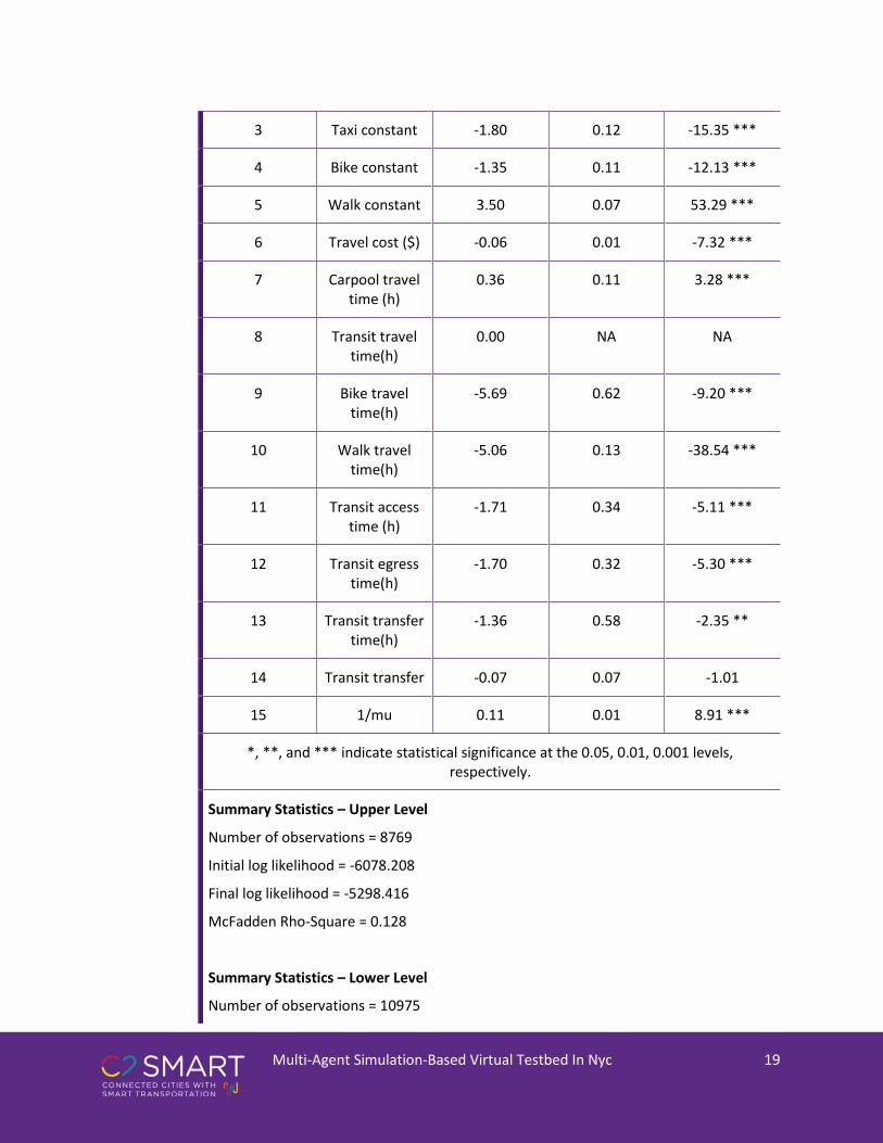
Multi-Agent Simulation-Based Virtual Testbed In Nyc 19
3 Taxi constant -1.80 0.12 -15.35 ***
4 Bike constant -1.35 0.11 -12.13 ***
5 Walk constant 3.50 0.07 53.29 ***
6 Travel cost ($) -0.06 0.01 -7.32 ***
7 Carpool travel time (h)
0.36 0.11 3.28 ***
8 Transit travel time(h)
0.00 NA NA
9 Bike travel time(h)
-5.69 0.62 -9.20 ***
10 Walk travel time(h)
-5.06 0.13 -38.54 ***
11 Transit access time (h)
-1.71 0.34 -5.11 ***
12 Transit egress time(h)
-1.70 0.32 -5.30 ***
13 Transit transfer time(h)
-1.36 0.58 -2.35 **
14 Transit transfer -0.07 0.07 -1.01
15 1/mu 0.11 0.01 8.91 ***
*, **, and *** indicate statistical significance at the 0.05, 0.01, 0.001 levels, respectively.
Summary Statistics – Upper Level
Number of observations = 8769
Initial log likelihood = -6078.208
Final log likelihood = -5298.416
McFadden Rho-Square = 0.128
Summary Statistics – Lower Level
Number of observations = 10975

Multi-Agent Simulation-Based Virtual Testbed In Nyc 20
Initial log likelihood = -16503.397
Final log likelihood = -7851.371
McFadden Rho-Square = 0.524
Table 4. Estimation results of nested logit model for both segments
We calculated the value of time (VOT) in Manhattan segment by computing 𝛽𝑡,𝑡𝑟𝑎𝑛𝑠𝑖𝑡
𝛽𝑐𝑜𝑠𝑡= $29/ℎ. This
value is higher than the $22.87/hr reported in Lam and Small (2001), which makes sense when
considering inflation and higher cost of living in Manhattan. The VOT for non-Manhattan is not reported
since it is not statistically significant.
Subsection 3.3.3: Smartphone Ownership Model and Mode Choice Update
Since the 2010/2011 RHTS didn’t include choices of FHV and Citi Bike, we need to update our model to
incorporate these two choices for our 2016 baseline model. Considering the choice of these two modes
is highly correlated to the ownership of smartphone, we estimated a smartphone ownership model for
NYC first.
The data comes from ACS household and person sample records (U.S. Census Bureau, 2016). Revealed
preference data for smartphones is only available in household records, so we use single-person
household records and match them to person records to obtain personal attributes. To be consistent
with the data available from RHTS, the person’s age, income and work status are selected as attributes.
All the attributes are categorical and have the same classifications as in RHTS. The final estimated utility
function specification for each individual 𝑛 choosing to own a smartphone is shown in Eq. (3.4) relative
to 𝑉𝑛𝑜,𝑛 = 0.
𝑽𝒚𝒆𝒔,𝒏 = 𝑪𝒚𝒆𝒔 + 𝜷𝒊𝒏𝒄𝟏× 𝒊𝒏𝒄𝟏,𝒏 + 𝜷𝒊𝒏𝒄𝟑
× 𝒊𝒏𝒄𝟑,𝒏 + 𝜷𝒊𝒏𝒄𝟒× 𝒊𝒏𝒄𝟒,𝒏 + 𝜷𝒂𝒈𝒆𝟓𝟔
× 𝒂𝒈𝒆𝟓𝟔,𝒏
+ 𝜷𝒂𝒈𝒆𝟕× 𝒂𝒈𝒆𝟕,𝒏 + 𝜷𝒘𝒐𝒓𝒌 × 𝒘𝒐𝒓𝒌𝒏
(3.4)
where 𝐶𝑦𝑒𝑠 is an alternative-specific constant of having the smartphone, 𝑖𝑛𝑐𝑖,𝑛 is a binary variable for
inclusion in annual income category 𝑖 (1: below $30K, 3: $75K-99.9K, 4: above $100K) for person 𝑛,
𝑎𝑔𝑒𝑖,𝑛 is a binary variable for inclusion in age category 𝑖 (56: 35-64, 7: older than 75) for person 𝑛, and
𝑤𝑜𝑟𝑘𝑛 indicates whether person 𝑛 works (1) or not (0).
We estimate the binary logit model using the open-source software PandasBiogeme (Bierlaire, 2018).
The estimation was run on a desktop with Intel Xeon 3.5 GHz and 125 GB RAM. Table 5 shows the
results of the estimated model. The coefficients of higher ages (group 5&6, and 7) are negative, which

Multi-Agent Simulation-Based Virtual Testbed In Nyc 21
indicates that elderly people are less likely to own a smartphone. And people with higher income or with
jobs are more likely to own a smartphone.
Variable name Coefficient estimate Standard error t statistic
Alt. Spec. Constant 1.75 0.138 12.7 ***
Age groups 5 & 6 -1.48 0.122 -12.1 ***
Age group 7 -2.63 0.126 -20.8 ***
Income group 1 -0.478 0.0679 -7.04 ***
Income group 3 0.641 0.125 5.11 ***
Income group 4 0.789 0.113 6.96 ***
Work status 1.08 0.0681 15.9 ***
*, **, and *** indicate statistical significance at the 0.05, 0.01, 0.001 levels, respectively.
Summary Statistics
Number of observations = 8030
Initial log likelihood = -5565.972
Final log likelihood = -3911.692
McFadden Rho-Square = 0.297
Table 5. Results of coefficients of Smart Phone ownership model
We updated the model to incorporate new mobility services. According to the synthetic population in
2016, the total number of daily trips is 30.5M, excluding the FHV and Citi Bike trip counts. The total daily
trips from 2010/2011 RHTS is 23.8M. The total daily trips increased by 28.33% from 2011 to 2016, so we
expanded the trips in 2011 by this factor to fit for 2016.
The probability of owning a smartphone obtained from the previous model was regarded as the
availability of FHV. The probability of choosing FHV is shown in Eq. (3.5). 𝑃𝑖,𝑘(𝐹𝐻𝑉) represents the
probability of choosing FHV for trip 𝑘 in tour 𝑖, 𝑉6,𝑖,𝑘 is identical to that of choosing taxi except for the
alternative specific constant which needs to be estimated, i.e. 𝑉6,𝑖,𝑘 = 𝛽6,𝐶 + 𝛽𝑐𝑜𝑠𝑡 × 𝐶𝑜𝑠𝑡𝑖,𝑘,6 +
𝛽𝑡𝑖𝑚𝑒,3 × 𝑇𝑖𝑚𝑒𝑖,𝑘,6, and 𝑃𝑆𝑀,𝑖(𝑦𝑒𝑠) is the probability of owning a smartphone in tour 𝑖. The 𝑇𝑖𝑚𝑒𝑖,𝑘,6

Multi-Agent Simulation-Based Virtual Testbed In Nyc 22
for FHV is assumed to be 80% that of taxi, resulting in 2.4 minutes in Manhattan and 4 minutes outside
Manhattan.
𝑃𝑖,𝑘(𝐹𝐻𝑉) = 𝑃𝑖,𝑘(𝐹𝐻𝑉|𝑁2) × 𝑃𝑖(𝑁2) × 𝑃𝑆𝑀,𝑖(𝑦𝑒𝑠)
=𝑒𝑉6,𝑖,𝑘
∑ (𝑒𝑉𝑗,𝑖,𝑘)𝐽∗
𝑗
×𝐸[𝑉𝑁2,𝑖]
𝐸[𝑉𝑁2,𝑖] + 𝑒𝑉𝑁1,𝑖×
𝑒𝑉𝑦𝑒𝑠
𝑒𝑉𝑦𝑒𝑠 + 1
(3.5)
The presence of FHV also impacts other modes because it affects the choice set. The probability of
choosing each mode except FHV is calculated with Eq. (3.6). 𝑃𝑖,𝑘(𝑚) denotes the probability of choosing
mode 𝑚 (excluding FHV) for trip 𝑘 in tour 𝑖. Since the probability of owning a smartphone is interpreted
as the availability of FHV, the probability of choosing each mode is calculated as the expected
probability conditional on owning a smartphone. 𝑃𝑖,𝑘(𝑚|𝑁2) × 𝑃𝑖(𝑁2) includes FHV in the choice set
whereas 𝑃′𝑖,𝑘(𝑗|𝑁2) × 𝑃′
𝑖(𝑁2) does not.
𝑃𝑖,𝑘(𝑚) = 𝑃𝑖,𝑘(𝑚|𝑁2) × 𝑃𝑖(𝑁2) × 𝑃𝑆𝑀,𝑖(𝑦𝑒𝑠) + 𝑃′𝑖,𝑘(𝑗|𝑁2) × 𝑃′
𝑖(𝑁2) × (1 − 𝑃𝑆𝑀,𝑖(𝑦𝑒𝑠))
=𝑒𝑉𝑚,𝑖,𝑘
∑ (𝑒𝑉𝑗,𝑖,𝑘)𝐽∗
𝑗
×𝐸[𝑉𝑁2,𝑖]
𝐸[𝑉𝑁2,𝑖] + 𝑒𝑉𝑁1,𝑖×
𝑒𝑉𝑦𝑒𝑠
𝑒𝑉𝑦𝑒𝑠 + 1
+𝑒𝑉𝑚,𝑖,𝑘
∑ (𝑒𝑉𝑗,𝑖,𝑘)𝐽∗
𝑗≠6
×𝐸[𝑉𝑁2,𝑖]𝑗≠6
𝐸[𝑉𝑁2,𝑖]𝑗≠6+ 𝑒𝑉𝑁1,𝑖
×1
𝑒𝑉𝑦𝑒𝑠 + 1, ∀𝑚 ∈ 𝐽∗ 𝑎𝑛𝑑 𝑚 ≠ 6
(3.6)
The utility of the Citi Bike choice is shown in Eq. (3.7).
𝑉𝑖,𝑘,7 = 𝛽7,𝐶 + 𝛽𝑐𝑜𝑠𝑡 ∗ 𝐶𝑜𝑠𝑡𝑖,𝑘,7 + 𝛽𝑡𝑖𝑚𝑒,4 ∗ 𝑇𝑖𝑚𝑒𝑖,𝑘,7 + 𝛽𝑠𝑚𝑎𝑟𝑡𝑝ℎ𝑜𝑛𝑒 ∗ 𝑃𝑆𝑀,𝑖(𝑦𝑒𝑠) (3.7)
In summary, we need to estimate the following parameters for the two emerging mobility modes:
𝛽6,𝐶 , 𝛽𝑠𝑚𝑎𝑟𝑡𝑝ℎ𝑜𝑛𝑒 , 𝛽7,𝐶, for two different segments, Manhattan and non-Manhattan (six parameters in
total).

Multi-Agent Simulation-Based Virtual Testbed In Nyc 23
Estimation of the three parameters is done using the aggregation of the choices from the two market
segments in 2016 compared to observed trips generated per zone, using nonlinear least squares
regression (NLSR). The objective of the NLSR estimation is shown in Eq. (3.8).
min 𝑧𝛽6,𝐶,𝛽𝑠𝑚𝑎𝑟𝑡𝑝ℎ𝑜𝑛𝑒,𝛽7,𝐶
= ∑[(𝑇𝑟𝑖𝑝𝑝𝑟𝑒,𝑖,𝐹𝐻𝑉 − 𝑇𝑟𝑖𝑝𝑜𝑏𝑠,𝑖,𝐹𝐻𝑉)2+ (𝑇𝑟𝑖𝑝𝑝𝑟𝑒,𝑖,𝐶𝐵 − 𝑇𝑟𝑖𝑝𝑜𝑏𝑠,𝑖,𝐶𝐵)
2]
𝑁
𝑖=1
(3.8)
where 𝑇𝑟𝑖𝑝𝑝𝑟𝑒,𝑖,𝐹𝐻𝑉 = 𝑇𝑟𝑖𝑝𝑝𝑟𝑒,𝑖,𝐹𝐻𝑉,𝑀𝑎𝑛ℎ𝑎𝑡𝑡𝑎𝑛 + 𝑇𝑟𝑖𝑝𝑝𝑟𝑒,𝑖,𝐹𝐻𝑉,𝑛𝑜𝑛𝑀𝑎𝑛ℎ𝑎𝑡𝑡𝑎𝑛, and 𝑁 = {1,2,… ,1622} is
the set of TAZs in NYC. The NLSR is run in MATLAB 2016a on a desktop with Intel® Core™ i7-6700 CPU @
3.40 GHZ, 16 GB RAM. The calculation time is 531 seconds.
A bootstrapping method was adopted to measure the statistical significance of the estimated
coefficients. The coefficient set generated by bootstrapping (Chernick and LaBudde, 2014) has 50
bootstrap samples for each coefficient. The estimated coefficients from the NLSR and the statistical
significance tests are shown in Table 6. The approximate t-stats based on bootstrapping suggest the
coefficients are statistically significant.
Bootstrap
Segment No. Variable
name Estimated
value Lower bound
Upper bound
Standard Error
t-stat
Manhattan
1 Citi Bike Constant
-0.35 -0.53 -0.11 0.09 -3.89***
2 FHV Constant
0.80 0.69 0.92 0.06 13.33***
3 Smartphone -0.34 -0.67 -0.06 0.10 -3.40***
Non-
Manhattan
4 Citi Bike Constant
-1.91 -2.64 -1.67 0.20 -9.55***
5 FHV Constant
-3.46 -3.89 -2.74 0.21 -16.48***
6 Smartphone -1.51 -2.11 -1.34 0.16 -9.44***
# of Observations
1622

Multi-Agent Simulation-Based Virtual Testbed In Nyc 24
RMSE (%CV) FHV: 401.83 trips/zone (154% NYC, 51% Manhattan)
Citi Bike: 59.80 trips/zone (54%)
*, **, and *** indicate statistical significance at the 0.05, 0.01, 0.001 levels, respectively.
Table 6. Estimated parameters and confidence intervals for FHV and Citi Bike
To validate the model, we compared the aggregated mode share from the synthetic population to the
2017 Citywide Mobility Survey (CMS) from NYC DOT. The results are presented in Figure 12. Comparing
to the mode share of 2011 RHTS, the prediction of synthetic population is closer to the 2017 CMS.
Figure 12. Aggregated mode share of 2011 RHTS, synthetic population and 2017 CMS
Section 4: Baseline Model Calibration
As introduced in Section 2, MATSim uses a queue model to simulate traffic dynamics. We calibrate the
road network in the baseline model to capture factors not considered: e.g. arterial traffic systems, non-
resident (tourist) trips, truck deliveries. The synthetic population’s mode choice model also needs to be
adjusted to fit the MNL-oriented model structure from the nested logit model.

Multi-Agent Simulation-Based Virtual Testbed In Nyc 25
Subsection 4.1: Data Preparation
Subsection 4.1.1: Modal Networks
The Modal networks consists of a road network transformed from Open Street Map (OSM) data and a
transit network generated from GTFS data. The transformation of road network is conducted via the
open-source Java-based network edit tool JOSM (JOSM, 2018). The OSM data is extracted in November
2018. The road network is shown in Figure 13. We classified the links of road network to two categories:
Arterial link and Freeway link. If the free flow speed of a link is above 33.33 m/s (about 75 mph), it
belongs to a Freeway link, otherwise it is an Arterial link.
The transit network is generated from GTFS data (MTA, 2018) in September 2016. The stop locations,
operation schedules and timetables are the same as in the historical data. Vehicle capacities are also
calibrated. We combined the transit network with the road network using MATSim extension
“pt2matsim”. The combined modal network is presented in Figure 14. The routes of transit lines are
artificially generated according to the distances between stations and operation timetables, instead of
searching in the road network. As a result, the transit assignment is simulated on dedicated links.
Figure 13. Road network from OSM data

Multi-Agent Simulation-Based Virtual Testbed In Nyc 26
Figure 14. Modal network of NYC
Subsection 4.1.2: Extended Travel Demand
In Section 3, we developed the synthetic population of NYC with personal information, travel agendas
and mode choices. However, this population only incorporates city residents. Those who live outside the
city but travel to NYC are not included, which would lead to less volumes in some areas. Therefore, we
generated a subpopulation of those non-residential travelers to compensate for the missing volumes.
The subpopulation is duplicated from the 2011 RHTS, keeping the agendas the same. The modes are
aggregated to walking, driving and transit. For the trips cross the boundary of the city, the
origin/destination of inside/outside trips will be switched to the nearest gateway by modes. The
locations of all the gateways are shown in Figure 15. In the end, a 1.18M population was added to the
simulation with 3.04M trips.

Multi-Agent Simulation-Based Virtual Testbed In Nyc 27
Figure 15. Gateway locations around the city
Subsection 4.1.3: Activity and Travel Parameters in MATSim
In MATSim, each agent has multiple plans in a day and selects one to execute among them. To evaluate
the plans, a score is calculated for each plan, which is similar to the mode utility in the mode choice
model but incorporates the additional utility (score) of activities (Nagel et al., 2016). The basic function
of calculating the plan score is shown in Eq. (4.1).
𝑆𝑝𝑙𝑎𝑛 = ∑ 𝑆𝑎𝑐𝑡,𝑞 + ∑ 𝑆𝑡𝑟𝑎𝑣,𝑚𝑜𝑑𝑒(𝑞)
𝑁−1
𝑞=0
𝑁−1
𝑞=0
(4.1)
where 𝑁 is the number of activities in the plan, 𝑆𝑎𝑐𝑡,𝑞 refers to the score of activity 𝑞 and 𝑆𝑡𝑟𝑎𝑣,𝑚𝑜𝑑𝑒(𝑞)
represents the score of trip after activity 𝑞 by 𝑚𝑜𝑑𝑒(𝑞). The last activity is combined with the first one
to have the same number of activities and trips. The score functions are shown in Eqs. (4.2a) – (4.2d).
𝑆𝑑𝑢𝑟,𝑞 = 𝛽𝑑𝑢𝑟 ∗ 𝑡𝑡𝑦𝑝,𝑞 ∗ ln (𝑡𝑑𝑢𝑟,𝑞 𝑡0,𝑞)⁄ (4.2a)
𝑆𝑤𝑎𝑖𝑡,𝑞 = 𝛽𝑤𝑎𝑖𝑡 ∗ 𝑡𝑤𝑎𝑖𝑡,𝑞 (4.2b)

Multi-Agent Simulation-Based Virtual Testbed In Nyc 28
𝑆𝑙𝑎𝑡𝑒 𝑎𝑟𝑟,𝑞 = {𝛽𝑙𝑎𝑡𝑒 𝑎𝑟𝑟 ∗ (𝑡𝑠𝑡𝑎𝑟𝑡,𝑞 − 𝑡𝑙𝑎𝑡𝑒𝑠𝑡 𝑎𝑟𝑟,𝑞), 𝑖𝑓 𝑡𝑠𝑡𝑎𝑟𝑡,𝑞 > 𝑡𝑙𝑎𝑡𝑒𝑠𝑡 𝑎𝑟𝑟,𝑞
0, 𝑜𝑡ℎ𝑒𝑟𝑤𝑖𝑠𝑒
(4.2c)
𝑆𝑒𝑎𝑟𝑙𝑦 𝑑𝑒𝑝,𝑞 = {𝛽𝑒𝑎𝑟𝑙𝑦 𝑑𝑒𝑝 ∗ (𝑡𝑒𝑎𝑟𝑙𝑖𝑒𝑠𝑡 𝑑𝑒𝑝,𝑞 − 𝑡𝑒𝑛𝑑,𝑞 ), 𝑖𝑓 𝑡𝑒𝑎𝑟𝑙𝑖𝑒𝑠𝑡 𝑑𝑒𝑝,𝑞 > 𝑡𝑒𝑛𝑑,𝑞
0, 𝑜𝑡ℎ𝑒𝑟𝑤𝑖𝑠𝑒
(4.2d)
𝑆𝑠ℎ𝑜𝑟𝑡 𝑑𝑢𝑟,𝑞 = {𝛽𝑠ℎ𝑜𝑟𝑡 𝑑𝑢𝑟 ∗ (𝑡𝑠ℎ𝑜𝑟𝑡 𝑑𝑢𝑟,𝑞 − 𝑡𝑑𝑢𝑟,𝑞), 𝑖𝑓 𝑡𝑠ℎ𝑜𝑟𝑡 𝑑𝑢𝑟,𝑞 > 𝑡𝑑𝑢𝑟,𝑞
0, 𝑜𝑡ℎ𝑒𝑟𝑤𝑖𝑠𝑒
(4.2e)
where 𝑡𝑡𝑦𝑝,𝑞 is the typical duration of activity 𝑞, 𝑡𝑑𝑢𝑟,𝑞 is the actual duration of activity 𝑞, 𝑡0,𝑞 is the
duration when the utility of activity 𝑞 starts to be positive. 𝑡0,𝑞 is set to 𝑡𝑡𝑦𝑝,𝑞 × exp (−10ℎ/𝑡𝑡𝑦𝑝,𝑞)
according to Rieser et al. (2014). We have five activity types defined in MATSim: Home, Work, School,
University and Secondary. MATSim defines the maximum durations for the whole population by activity
type: we set the maximum durations of the activities as 8h, 8h, 8h, 1h and 1h correspondingly. 𝑡𝑤𝑎𝑖𝑡,𝑞 is
the wait time before activity 𝑞 starts, 𝑡𝑠𝑡𝑎𝑟𝑡,𝑞 is the actual start time of activity 𝑞, 𝑡𝑙𝑎𝑡𝑒𝑠𝑡 𝑎𝑟𝑟,𝑞 is the latest
start time of activity 𝑞 without penalty, 𝑡𝑒𝑛𝑑,𝑞 is the actual end time of activity 𝑞, 𝑡𝑒𝑎𝑟𝑙𝑖𝑒𝑠𝑡 𝑑𝑒𝑝,𝑞 is the
earliest possible leaving time of activity 𝑞, 𝑡𝑠ℎ𝑜𝑟𝑡 𝑑𝑢𝑟,𝑞 is the shortest possible duration of activity 𝑞. Eq.
(4.2a) defines the score of performing an activity, which is usually positive. Eq. (4.2b) represents the wait
penalty. Eq. (4.2c) is the penalty of late arrival, Eq. (4.2d) is the penalty of early departure, and Eq. (4.2e)
denotes the penalty for a “too short” activity. 𝛽𝑤𝑎𝑖𝑡, 𝛽𝑒𝑎𝑟𝑙𝑦 𝑑𝑒𝑝 , 𝛽𝑠ℎ𝑜𝑟𝑡 𝑑𝑢𝑟 are recommended to be 0
according to Nagel et al. (2016), if no data is available to determine those parameters. 𝛽𝑑𝑢𝑟 is set to be
the same as the positive value of the parameter for travel time of driving alone, and the 𝛽𝑙𝑎𝑡𝑒 𝑎𝑟𝑟 is
determined relative to the parameter of travel time of driving alone according to Small (1982). Small
(1982) proposed a scheduling model for work trips and the results indicated that the parameter of
schedule delay is about 2.39 times of travel time. We use this to estimate a 𝛽𝑙𝑎𝑡𝑒 𝑎𝑟𝑟 = −4.19. The
parameters used to calculate the activity score in MATSim-NYC are presented in Table 7. Since 𝛽𝑑𝑢𝑟 is
assumed in order to have agents try to maximize their durations, we make sure to omit the duration
attribute from the score calculations when determining consumer surplus (i.e. the consumer surplus
measure reported in our results captures travel disutilities and schedule delays, not activity participation
utility).
𝜷𝒅𝒖𝒓 𝜷𝒘𝒂𝒊𝒕 𝜷𝒍𝒂𝒕𝒆 𝒂𝒓𝒓 𝜷𝒆𝒂𝒓𝒍𝒚 𝒅𝒆𝒑 𝜷𝒔𝒉𝒐𝒓𝒕 𝒅𝒖𝒓
1.75 0 -4.19 0 0
Table 7. Parameters for activity score in MATSim
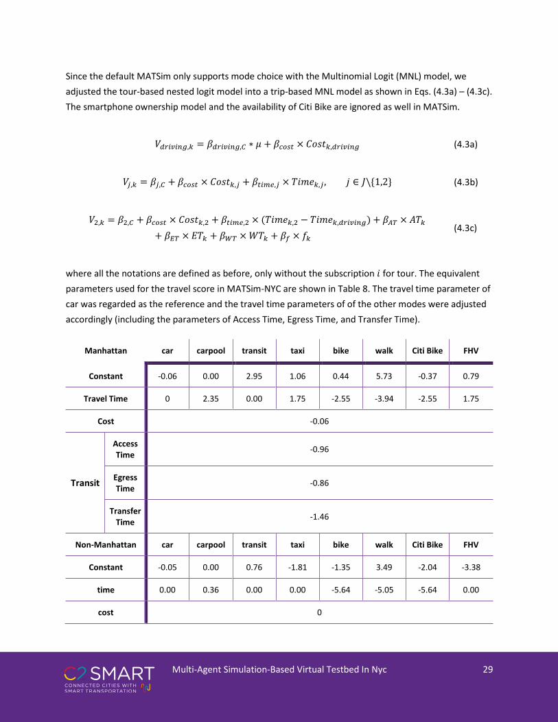
Multi-Agent Simulation-Based Virtual Testbed In Nyc 29
Since the default MATSim only supports mode choice with the Multinomial Logit (MNL) model, we
adjusted the tour-based nested logit model into a trip-based MNL model as shown in Eqs. (4.3a) – (4.3c).
The smartphone ownership model and the availability of Citi Bike are ignored as well in MATSim.
𝑉𝑑𝑟𝑖𝑣𝑖𝑛𝑔,𝑘 = 𝛽𝑑𝑟𝑖𝑣𝑖𝑛𝑔,𝐶 ∗ 𝜇 + 𝛽𝑐𝑜𝑠𝑡 × 𝐶𝑜𝑠𝑡𝑘,𝑑𝑟𝑖𝑣𝑖𝑛𝑔 (4.3a)
𝑉𝑗,𝑘 = 𝛽𝑗,𝐶 + 𝛽𝑐𝑜𝑠𝑡 × 𝐶𝑜𝑠𝑡𝑘,𝑗 + 𝛽𝑡𝑖𝑚𝑒,𝑗 × 𝑇𝑖𝑚𝑒𝑘,𝑗, 𝑗 ∈ 𝐽\{1,2} (4.3b)
𝑉2,𝑘 = 𝛽2,𝐶 + 𝛽𝑐𝑜𝑠𝑡 × 𝐶𝑜𝑠𝑡𝑘,2 + 𝛽𝑡𝑖𝑚𝑒,2 × (𝑇𝑖𝑚𝑒𝑘,2 − 𝑇𝑖𝑚𝑒𝑘,𝑑𝑟𝑖𝑣𝑖𝑛𝑔) + 𝛽𝐴𝑇 × 𝐴𝑇𝑘
+ 𝛽𝐸𝑇 × 𝐸𝑇𝑘 + 𝛽𝑊𝑇 × 𝑊𝑇𝑘 + 𝛽𝑓 × 𝑓𝑘 (4.3c)
where all the notations are defined as before, only without the subscription 𝑖 for tour. The equivalent
parameters used for the travel score in MATSim-NYC are shown in Table 8. The travel time parameter of
car was regarded as the reference and the travel time parameters of of the other modes were adjusted
accordingly (including the parameters of Access Time, Egress Time, and Transfer Time).
Manhattan car carpool transit taxi bike walk Citi Bike FHV
Constant -0.06 0.00 2.95 1.06 0.44 5.73 -0.37 0.79
Travel Time 0 2.35 0.00 1.75 -2.55 -3.94 -2.55 1.75
Cost -0.06
Transit
Access Time
-0.96
Egress Time
-0.86
Transfer Time
-1.46
Non-Manhattan car carpool transit taxi bike walk Citi Bike FHV
Constant -0.05 0.00 0.76 -1.81 -1.35 3.49 -2.04 -3.38
time 0.00 0.36 0.00 0.00 -5.64 -5.05 -5.64 0.00
cost 0
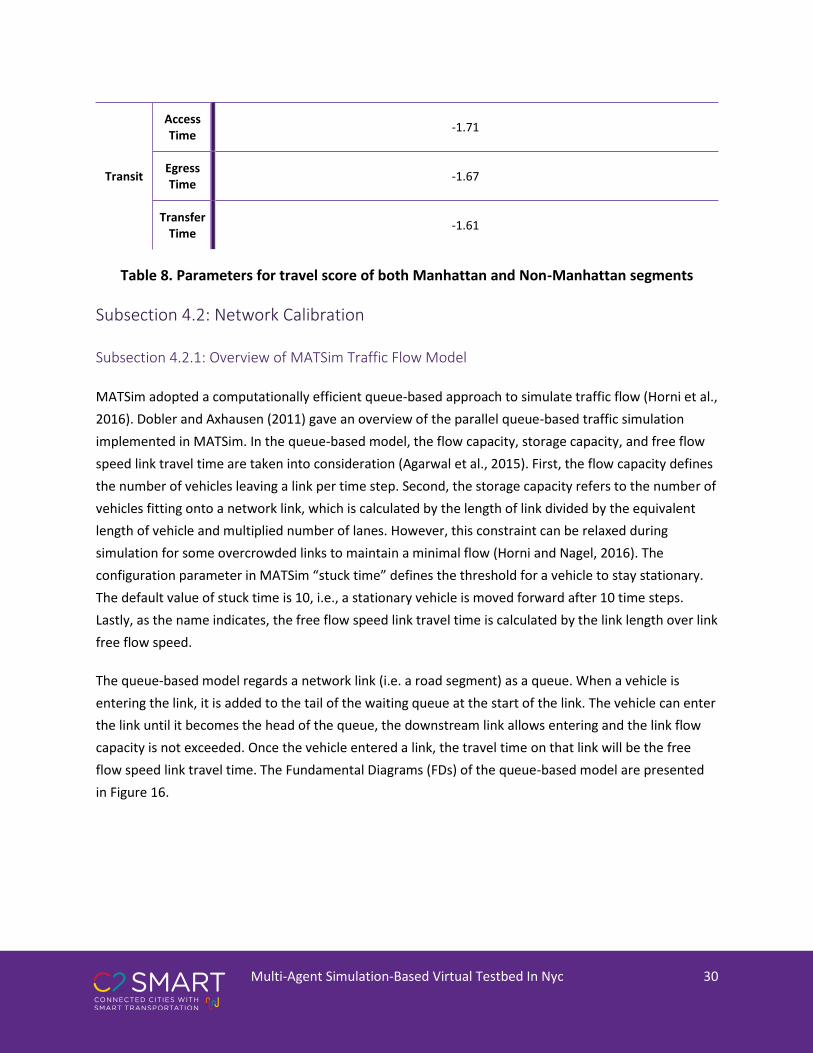
Multi-Agent Simulation-Based Virtual Testbed In Nyc 30
Transit
Access Time
-1.71
Egress Time
-1.67
Transfer Time
-1.61
Table 8. Parameters for travel score of both Manhattan and Non-Manhattan segments
Subsection 4.2: Network Calibration
Subsection 4.2.1: Overview of MATSim Traffic Flow Model
MATSim adopted a computationally efficient queue-based approach to simulate traffic flow (Horni et al.,
2016). Dobler and Axhausen (2011) gave an overview of the parallel queue-based traffic simulation
implemented in MATSim. In the queue-based model, the flow capacity, storage capacity, and free flow
speed link travel time are taken into consideration (Agarwal et al., 2015). First, the flow capacity defines
the number of vehicles leaving a link per time step. Second, the storage capacity refers to the number of
vehicles fitting onto a network link, which is calculated by the length of link divided by the equivalent
length of vehicle and multiplied number of lanes. However, this constraint can be relaxed during
simulation for some overcrowded links to maintain a minimal flow (Horni and Nagel, 2016). The
configuration parameter in MATSim “stuck time” defines the threshold for a vehicle to stay stationary.
The default value of stuck time is 10, i.e., a stationary vehicle is moved forward after 10 time steps.
Lastly, as the name indicates, the free flow speed link travel time is calculated by the link length over link
free flow speed.
The queue-based model regards a network link (i.e. a road segment) as a queue. When a vehicle is
entering the link, it is added to the tail of the waiting queue at the start of the link. The vehicle can enter
the link until it becomes the head of the queue, the downstream link allows entering and the link flow
capacity is not exceeded. Once the vehicle entered a link, the travel time on that link will be the free
flow speed link travel time. The Fundamental Diagrams (FDs) of the queue-based model are presented
in Figure 16.

Multi-Agent Simulation-Based Virtual Testbed In Nyc 31
Figure 16. FDs of MATSim queue-based model (a) Flow vs Density and (b) Speed vs Density
The queue-based model ignores the intra-link interactions to improve the computational efficiency.
When a link is saturated, the flow stays the same in MATSim as long as the downstream link is open,
while in the real world, the flow goes down as the density increases. This assumes that the MATSim
equilibrium operates in a steady state where traffic would not be oversaturated. Speed, even though it
goes down with density after the link is saturated, is still higher than the real speed because vehicles
travel with free flow speed after entering a link. Improvements are made to address these limitations in
Section 6.
Subsection 4.2.2: Calibration framework
Since the storage capacity is always set large enough or relaxed by configuration, the link flow capacity
and free flow speed are the major attributes that influence the traffic flow simulation in MATSim. In the
MATSim-NYC model, the road network is transformed from OSM data which has imprecise link flow
capacities and free flow speeds and therefore cannot represent the real road network. Other factors
(e.g. arterial traffic system, non-resident (tourist) trips, truck deliveries, etc.) that affect the link flow
capacity and free flow speed are not incorporated due to limitations of the data. The road network
attributes (link flow capacity and free flow speed) need to be calibrated to make the simulation model
more realistic.
We defined two sets of parameters for those two major network attributes. Based on the queue-based
model, vehicles travel with unsaturated flow speed when entering a link. Therefore, the link unsaturated
flow speed parameters are calibrated first according to the INRIX speed data and then implemented in
the road network. The link capacity factors are perturbated iteratively to find the equilibrium of the
calibrated link capacity and unsaturated flow speed, which leads to a closer volume distribution
compared to the real traffic count. The overview of the process is shown in Figure 17.

Multi-Agent Simulation-Based Virtual Testbed In Nyc 32
Figure 17. The framework of calibration process
Subsection 4.2.3: Reference Data
The 2016 bridges/tunnels volumes data (NYCDOT,2016) and INRIX speed data in September 2016, from
DOT were used as the calibration reference data. The volumes data contains hourly average traffic
counts of 59 bridges/tunnels around the city on a typical weekday. The speed data includes observed 5-
minute speeds for 6,996 link segments across the city.
We selected 19 facilities from the volumes data to calibrate the road capacities, as shown in Error! R
eference source not found.. A screenline along East River was defined, as red curves shown in Error!
Reference source not found., which consists of Queensboro Bridge, Williamsburg Bridge, Queens
Midtown Tunnel, Manhattan Bridge, Brooklyn Bridge, and Hugh Carey Tunnel. The Hudson River
crossings are not considered since most of the trips are made by non-residents which are not sensitive
to the calibration of the road network.
ID Facility
1 Brooklyn Bridge
2 Ed Koch Queensboro Bridge
3 Williamsburg Bridge
4 Alexander Hamilton Bridge

Multi-Agent Simulation-Based Virtual Testbed In Nyc 33
5 Macombs Dam Bridge
6 Madison Avenue Bridge
7 University Heights Bridge
8 Washington Bridge
9 Willis Avenue Bridge
10 145th Street Bridge
11 Hugh L. Carey Tunnel
12 Queens-Midtown Tunnel
13 Robert F. Kennedy Memorial Bridge Manhattan Plaza
14 Robert F. Kennedy Memorial Bridge Bronx Plaza
15 Verrazzano-Narrows Bridge
16 George Washington Bridge
17 Holland Tunnel
18 Lincoln Tunnel
19 Manhattan Bridge
Table 9. List of traffic count facilities

Multi-Agent Simulation-Based Virtual Testbed In Nyc 34
Figure 18. Select facilities for link capacity calibration and East River screenline
For the speed calibration, we took the average hourly speed on weekdays of September, 2016, as
reference. Figure 19 presents the distribution of average observed speed at 12 AM.
Figure 19. Distribution of average hourly speed at 12 AM from INRIX data

Multi-Agent Simulation-Based Virtual Testbed In Nyc 35
Subsection 4.2.4: Link Unsaturated Flow Speed Calibration
The default link free flow speed in MATSim is fixed across a day, while the speed from INRIX data varies
with time. We adopted a time-variant network to capture the variation of link free flow speed in our
simulation. Six time periods are defined for one day: 6 - 9 AM, 9 AM - 12 PM, 12 - 3 PM, 3 - 6 PM, 6 -
9PM and 9 PM - 6 AM. Different speed factors were applied to links according to link types (defined in
Section 4.1.1) and time. Denote 𝐿 = {1,2}, where 1 is freeway and 2 is arterial, and 𝑇 = {1,2,3,4,5,6}
refers to six time periods correspondingly.
First, the average speed data from INRIX were aggregated by link type and time period (Table 10). We
can calculate the link speed factors of each freeway link as Eq. (4.4).
𝑓1,𝑡𝑠 𝑣1
0 = 𝑣1,𝑡𝑜𝑏 , 𝑡 ∈ 𝑇 (4.4)
where 𝑣1,𝑡𝑜𝑏 refers to the average observed speed for the freeway link in time period 𝑡, and 𝑣1
0 represents
the default free flow speed for the freeway link.
6AM-9AM 9AM-12PM 12PM-3PM 3PM-6PM 6PM-9PM 9PM-12AM
Freeway 36.88 37.93 37.61 33.05 36.25 42.41
Arterial 14.10 13.42 13.11 12.80 13.91 15.34
Table 10. Average observed speed in each time period for Freeway and Arterial links (mph)
For Arterial links, further adjustments are needed due to high variation in free flow speed. A set of sub-
categories 𝐽 = {1,2,3} is used to represent arterial links with free flow speeds 22.2 m/s, 15.0 m/s and
8.3m/s, respectively. To adjust the link speed as close to observed speed as possible, we applied
different link speed factors to corresponding sub-categories of arterial links using Eq. (4.5).
𝑓2,𝑡,𝑗𝑠 𝑣2,𝑗
0 = 𝑣2,𝑡𝑜𝑏 , 𝑡 ∈ 𝑇, 𝑗 ∈ 𝐽 (4.5)
where 𝑣2,𝑗0 is the default link free speed for link sub-category 𝑗.

Multi-Agent Simulation-Based Virtual Testbed In Nyc 36
Subsection 4.2.3: Link Capacity Calibration
After the free flow speeds are adjusted to accommodate time-varying conditions like non-resident
traffic and signal control, the next step is the capacity calibration. Based on the time variant network
feature of MATSim, a link behaves according to Eq. (4.6).
𝐶𝑙,𝑡𝑠𝑖𝑚 = 𝐶𝑙
0𝑓𝑙,𝑡𝑐 (4.6)
where 𝐶𝑙,𝑡𝑠𝑖𝑚 is the link flow capacity in simulation for facility type 𝑙 ∈ 𝐿 in time period 𝑡 ∈ 𝑇, 𝐶𝑙
0 is the
default link capacity for facility type 𝑙 ∈ 𝐿 from OSM, and 𝑓𝑙,𝑡𝑐 is a factor to adjust the capacity for a given
facility type 𝑙 ∈ 𝐿 in time period 𝑡 ∈ 𝑇. The storage capacities are unchanged from the default values
(average vehicle length set to 7.5 m). The flow capacities are used in a cellular automata model to
propagate traffic within the road network to output location volumes by time of day within one day. The
simulation then proceeds through multiple days with each subsequent day updating the travel choices
of the population and the cellular automata model updates the system performance based on the
propagation of the new day’s traffic. The resulting output of 𝑛 days of simulation is denoted as Ωn, i.e.
({𝑉𝑖,𝑡𝑠𝑖𝑚}) = Ωn(𝜃, 𝐼; 𝑓𝑠) for location 𝑖 at time period 𝑡. In our model there are 12 (2 types, 6 periods)
capacity parameters to be calibrated. The 19 locations in Error! Reference source not found. are used f
or the calibration.
The objective is to minimize the simulation error with respect to the observed data (Yu and Fan, 2017).
The loss function 𝐿(𝜃, 𝐼; 𝑓𝑠) is a response to a set of parameters and model input data 𝐼 given speed
factors 𝑓𝑠. It is shown in Eq. (4.7). 𝜃 is a generic term representing the set of flow capacity factors 𝑓𝑙,𝑡𝑐 .
min𝐿(𝜃, 𝐼; 𝑓𝑠) = ∑∑|𝑉𝑖,𝑡𝑜𝑏 − Ω(𝜃, 𝐼; 𝑓𝑠)|/𝑉𝑖,𝑡
𝑜𝑏
𝑡∈𝑇𝑖∈𝑁
(4.7)
where 𝑉𝑖,𝑡𝑜𝑏 and 𝑉𝑖,𝑡
𝑠𝑖𝑚 are the average observed volumes and average simulated volumes of location 𝑖 in
time period 𝑡.
To estimate the capacity parameters 𝜃 in Eq. (4.7), the approach of stochastic approximation (SA) is
applied (Robbins and Monro, 1951). The SA approach is an iterative algorithm to update the parameter
set. Let 𝜃𝑘 denote the estimate for 𝜃∗ at the 𝑘th iteration. The standard form of the update algorithm is
shown in Eq. (4.8), where 𝑔𝑘 is the gradient and 𝑎𝑘 is a step size at the 𝑘th iteration.

Multi-Agent Simulation-Based Virtual Testbed In Nyc 37
𝜃𝑘 = 𝜃𝑘−1 − 𝑎𝑘−1𝑔𝑘−1(𝜃𝑘−1) (4.8)
The general idea of the SA algorithm is to mimic the gradient search method used in deterministic
optimization problems, which requires a gradient of the loss function for the parameter update.
However, for a traffic simulation model, the analytical form of the gradient of Ω(𝜃, 𝐼; 𝑓𝑠) is not available
for calculation. A numerical approximation of the gradient is obtained instead. With an approximated
gradient, Equation (4.8) can be rewritten as Eq. (4.9).
𝜃𝑘 = 𝜃𝑘−1 − 𝑎𝑘−1�̂�𝑘−1(𝜃𝑘−1) (4.9)
A well-known method for gradient approximation is the finite-difference (FD) method (Dennis and
Schnabel, 1989). This method has two types, namely, one-sided and two-sided approximation. They are
shown as:
𝑔𝑘(�̂�𝑘) =
[ 𝐿(𝜃𝑘 + 𝑐𝑘𝑒1) − 𝐿(𝜃𝑘)
𝑐𝑘
⋮𝐿(𝜃𝑘 + 𝑐𝑘𝑒𝑝) − 𝐿(𝜃𝑘)
𝑐𝑘 ]
(4.10)
𝑔𝑘(�̂�𝑘) =
[ 𝐿(𝜃𝑘 + 𝑐𝑘𝑒1) − 𝐿(𝜃𝑘 − 𝑐𝑘𝑒1)
2𝑐𝑘
⋮𝐿(𝜃𝑘 + 𝑐𝑘𝑒𝑝) − 𝐿(𝜃𝑘 − 𝑐𝑘𝑒𝑝)
2𝑐𝑘 ]
(4.11)
where 𝑒𝑖 denotes a vector with a one in the 𝑖th place and zeros elsewhere. However, this method is not
computationally efficient for problems with an increasing parameter size. For example, if the number of
parameters is p, the one-sided approximation needed to calculate p+1 functions and the two-sided one
needs 2p functions. The computational effort increases linearly with the number of parameters. To
address this difficulty, the simultaneous perturbation stochastic approximation (SPSA) algorithm
provides a good alternative to the FD method.
The SPSA method (Spall, 1988, 1998a, 1998b) requires only two measurements to approximate the
gradient at each iteration regardless of the dimension of the parameters vector 𝜃. This is achieved as all

Multi-Agent Simulation-Based Virtual Testbed In Nyc 38
elements of the 𝜃𝑘 vector are varied simultaneously, instead of calculating the measurements one by
one for p+1 or 2p times like in the FD method. The formulation for SPSA algorithm is shown as:
𝑔𝑘(�̂�𝑘) =
[ 𝐿(𝜃𝑘 + 𝑐𝑘Δ𝑘) − 𝐿(𝜃𝑘 − 𝑐𝑘Δ𝑘)
2𝑐𝑘Δ𝑘1
⋮𝐿(𝜃𝑘 + 𝑐𝑘Δ𝑘) − 𝐿(𝜃𝑘 − 𝑐𝑘Δ𝑘)
2𝑐𝑘Δ𝑘𝑝 ]
=𝐿(𝜃𝑘 + 𝑐𝑘Δ𝑘) − 𝐿(𝜃𝑘 − 𝑐𝑘Δ𝑘)
2𝑐𝑘
[ Δ𝑘1
−1
Δ𝑘2−1
⋮Δ𝑘𝑝
−1]
(4.12)
The approximation function for each parameter is the same except the perturbation term. This means
the measurement of the loss function just needs to be calculated twice, 𝐿(𝜃𝑘 + 𝑐𝑘Δ𝑘) and
𝐿(𝜃𝑘 − 𝑐𝑘Δ𝑘). Compared with the FD method, this provides significant computational improvement for
optimization analysis. More detailed discussion of SPSA algorithm can be found refer in Spall (1988,
1998a, 1998b). The capacity calibration algorithm is summarized in Figure 17. The SPSA method from
Spall is shown in Algorithm 1.
Algorithm 1: SPSA (source: Spall (1988, 1998a, 1998b))
Input: initial vector of link capacity factors 𝜃0
0: Initialization
Set 𝑘 = 1, 𝛽, 𝛾, 𝑎, 𝐴, 𝑐 as initial values.
1: Generation of simultaneous perturbation vectors
Generate a 𝑝-dimension ∆𝑘 by Monte Carlo. Each element of ∆𝑘 is generated independently from a
Bernoulli ±1 distribution with probability of ½.
Calculate 𝑎𝑘 =𝑎
(𝑘+𝐴)𝛽 and 𝑐𝑘 =
𝑐
𝑘𝛾.
2: Gradient approximation

Multi-Agent Simulation-Based Virtual Testbed In Nyc 39
Calculate the gradient by Eq. (4.9).
3: Update 𝜃𝑘 estimation
Update 𝜃𝑘 by Eq. (4.6).
Terminate the algorithm when loss function in Eq. (4.9) reached the threshold or the maximum
iteration were reached, or set 𝑘 = 𝑘 + 1 and return step 1.
Output: final vector of link capacity factors 𝜃𝑘
The SPSA method was implemented in Java and run with the MATSim-NYC model. The initial coefficients
are 𝛽 = 0.602, 𝛾 = 0.101, 𝑎 = 0.16, 𝐴 = 3000, 𝑐 = 0.05. The initial value of the link flow capacity
factor is 0.6. The upper bound and lower bound of link capacity factors are set as 0.8 and 0.3 to make
sure the link capacities stay in a reasonable range. To save computation time for calibration, we ran only
𝑛 = 50 days in MATSim for each iteration of the calibration.
Subsection 4.3: Calibration Results
The calibration was running on a desktop with Intel(R) Xeon(R) CPU E5-2637 v4 @ 3.50GHz processors
and 128GB RAM. We ran the calibration for 6 iterations until the simulated screenline volumes were
observed to be close to the observed data. Each iteration took around 11 hours. The calibrated link
capacity factors are presented in Table 11.
6AM-9AM 9AM-12PM 12PM-3PM 3PM-6PM 6PM-9PM 9PM-12AM
Freeway 0.61 0.69 0.51 0.63 0.55 0.68
Arterial 0.59 0.51 0.57 0.50 0.46 0.68
Table 11. Calibrated link capacity factors for Freeway and Arterial links

Multi-Agent Simulation-Based Virtual Testbed In Nyc 40
Figure 20. Comparison of INRIX speed (observed) and simulated speed
As Figure 20 shows, the simulated average speed in each time period is close to the INRIX speed. For the
Freeway links, the relative difference is 7.2% on average, with the highest of 9.5%. For the Arterial links,
the relative difference is 17.1% on average, with the highest at 18.5%. The results of the Arterial links
are worse because the default free flow speeds of the Arterial links vary more.
Figure 21. Average simulated and real volume distribution of East River screenline across all
time periods
The simulated volumes of the screenlines are also close to the real traffic count. For the East River
screenline, the difference between the total daily simulated volumes and real volumes is only 2.6%. If
we look at different time periods, the relative difference is 10.3% on average, with the highest at 16.3%.

Multi-Agent Simulation-Based Virtual Testbed In Nyc 41
We also compared the calibration results of East River screenline with the NYBPM 2010 update
(Brinckerhoff, 2014). The results are presented in Table 12. The MATSim NYC model has the similar
difference of East River screenline with NYBPM, which is 2.6% to -2.4%.
East River screenline
NYBPM 2010 update -2.4%
MATSim NYC model 2.6%
Table 12. Differences between modeled daily volumes and real counts of NYBPM and
MATSim NYC model
Subsection 4.4: Validation
We validated the calibrated model by comparing the simulation output transit station ridership with
observed turnstile count data as well as with volumes on key corridors.
Subsection 4.4.1: Validation Data
Two data sources are adopted for validation: 2016 Average Weekday Subway Ridership data (MTA,
2018) and 2014-2018 Traffic Volume Counts data (NYC DOT, 2019). The subway ridership data
incorporates the average weekday ridership per subway station across the city. The ridership refers to
the number of passengers entering the station, including passengers transfer from other stations.
Passengers transferring in the same station are not incorporated. We selected 10 stations of the city as
reference (shown in Figure 22). The validation results of transit station ridership are presented in Table
13. The difference of total daily ridership is only 8%.

Multi-Agent Simulation-Based Virtual Testbed In Nyc 42
Figure 22. Subway locations for validation
Station Real Simulated Difference %
14 St - Union Square 106,718 97,825 -8%
Grand Central - 42 St 158,580 170,025 7%
Penn Station - 123 & ACE 173,108 256,825 48%
Times Square 202,363 191,425 -5%
Fulton St 85,440 83,025 -3%
Canal St 70,806 78,250 11%
59 St - Columbus Circle 73,836 75,050 2%
34 St - Herald Sq 125,682 124,500 -1%

Multi-Agent Simulation-Based Virtual Testbed In Nyc 43
Atlantic Av-Barclays Ctr (Brooklyn) 42,711 59,350 39%
Jackson Hts-Roosevelt Av (Queens) 52,296 41,200 -21%
Average 1,091,540 1,177,475 8%
Table 13. Comparison of simulated and observed daily ridership of 10 stations
The 2014-2018 Traffic Volume Counts data was collected by NYC DOT for validation of NYBPM. The data
consists of hourly volumes of 597 locations across the city from 2014 – 2018. To validate the MATSim
NYC model, the volume counts in 2016 of 15 locations are selected (listed in Table 14). As the red links
show in Figure 23, some locations (e.g. 3 AVENUE) have more than one count facility. When matched
with those facilities in the MATSim-NYC network, 42 links were selected. The daily volumes of the 42
links were compared and the relative difference between simulated volumes and real counts is 39.8% on
average. The median difference is 29%.
ID Location
1 10th Avenue
2 2nd Avenue
3 3rd Avenue
4 5th Avenue
5 9th Avenue
6 Canal Street
7 East 119th Street
8 FDR Drive
9 Grand Central Parkway
10 Grand Street
11 Madison Avenue
12 Northern Boulevard
13 West 29th Street

Multi-Agent Simulation-Based Virtual Testbed In Nyc 44
14 Long Island Expressway
15 Brooklyn-Queens Expressway
Table 14. Locations for link volume validation
Figure 23. Distribution of volume count facilities
Section 5: Scenario Analyses
We conducted five scenario analyses based on the calibrated baseline model in MATSim. Scenario One is
the impact analysis of the hypothetical set-up of a new Amazon HQ in Long Island City. Scenario Two is
the demand forecast of Citi Bike’s expansion plan. The analyses of those two scenarios are completed
based solely on the synthetic population and estimated tour-based mode choice model. Scenario Three
is the evaluation of the congestion pricing policy in CBD area of Manhattan. Scenario Four is the
implementation of the Brooklyn Queens Connector (BQX). Scenario Five is the deployment of
autonomous vehicles in Manhattan. The last three scenarios are tested on the calibrated simulation test
bed. The details of all scenarios are introduced in the rest of this section.
For our base model, we use the calibrated model with an adjustment for the fare price. Assume a
passenger pays $2.75 per transit trip (unlimited plan and free transfers are assumed to be priced into
that fare). The utility function of transit is adjusted and shown in Eq. (5.1) and (5.2). The disutility of
fixed transit fare per trip was added into the constant of the previous utility function of transit.

Multi-Agent Simulation-Based Virtual Testbed In Nyc 45
𝑉′2,𝑘 = 𝛽′2,𝐶 + 𝛽𝑡𝑖𝑚𝑒,2 × (𝑇𝑖𝑚𝑒𝑘,2 − 𝑇𝑖𝑚𝑒𝑘,𝑑𝑟𝑖𝑣𝑖𝑛𝑔) + 𝛽𝐴𝑇 × 𝐴𝑇𝑘 + 𝛽𝐸𝑇 × 𝐸𝑇𝑘 + 𝛽𝑊𝑇 × 𝑊𝑇𝑘
+ 𝛽𝑓 × 𝑓𝑘
(5.1)
𝛽′2,𝐶 = 𝛽2,𝐶 + 𝛽𝑐𝑜𝑠𝑡 ∗ 2.75 (5.2)
Subsection 5.1: Scenario One
Amazon planned to build a new HQ in Long Island City (LIC Development MOU, 2018). The project
expected to create 25,000 new jobs in ten years and up to 40,000 new jobs in fifteen years. Although
that decision has since been canceled (NBC, 2019), it presents a timely case study with well-defined
parameters to study its potential effect on travel patterns as NYC continues growing its technology
sector.
Figure 24. Original planned site of Amazon’s NYC Headquarters (LIC Development MOU, 2018)
We assume the new HQ will attract employees from the “professional, scientific, and technical services”
(PSTS), with North American Industry Code System (NAICS) code 54. The process flow of this scenario
analysis is shown in Figure 25. First, the population is expanded with the natural growth rate 0.3% (NYC
Planning, 2017) to predict the population in 2028. About 8,023 new people will join the PSTS industry for
the whole city under the natural growth, of which 8.01% (643 in total) are attracted by Amazon. The
reminder of 25,000 new jobs come from outside the city. Then, socio-demographic attributes and
agendas are randomly assigned to those increment of population. Amazon workers receive attributes

Multi-Agent Simulation-Based Virtual Testbed In Nyc 46
from PSTS industry while others receive attributes from other industries. Amazon workers have the
simplest agenda: 8:30AM from home to work and 5:30PM from work to home. Others take the agendas
as the same as the existing population excluding PSTS workers.
Figure 25. Process flow of experimental design
By using a synthetic population, we can adjust specific individuals by employment industry. As a result,
the spatial distribution of potential employees can be modeled as shown in
Figure 26.

Multi-Agent Simulation-Based Virtual Testbed In Nyc 47
Figure 26. Spatial distribution of home locations for workers in TAZ 362 (a) in 2016, and (b) in
2028 with Amazon HQ relocation
The mode choices of the increment of population are simulated based on the mode choice model. The
prediction is presented in Table 15. A dramatic increase is predicted with the new HQ. The demand for
taxi and FHV is expanded by more than four times, with the ridership of transit increased nearly three
times. This prediction can act as a reference for policymakers to plan the improvement of infrastructure
such as ensuring sufficient capacity for transit facilities nearby.
Driving Carpool Transit Taxi Bike Walk FHV Citi Bike
Total
Number of trips
2016 6519 1262 10,716 266 176 2144 143 34 21,260
2028 without Amazon
6749 1316 11,106 272 181 2220 145 37 22,026
2028 with
Amazon
20,081 3368 42,254 1393 848 3120 773 189 72,026
Change in percentage
2028 without Amazon
3% 4% 4% 2% 3% 3% 1% 8% 3%
2028 with
Amazon
208% 167% 294% 424% 382% 46% 441% 456% 239%
Table 15. Mode share of Amazon workers in 2016 and 2028

Multi-Agent Simulation-Based Virtual Testbed In Nyc 48
A further advantage of using a synthetic population is that a time-of-day analysis can be easily
conducted, as shown in

Multi-Agent Simulation-Based Virtual Testbed In Nyc 49
Figure 27. The new HQ is predicted to increase total trips from 5,000 to 8,000 in the morning peak and
from 3,000 to 8,000 in the afternoon peak. Late night trips would also expand.
Figure 27. Time-of-day distribution of inbound and outbound trips at TAZ 362 in 2028 (a)
without Amazon and (b) with Amazon
Subsection 5.2: Scenario Two
Citi Bike proposed plans in 2019 to expand its service area to double its size by 2023. The expansion plan
is shown in Figure 28. We estimated the demand attracted by the expanded service assuming that the
level of service of the system remains the same. The parameters estimated for the bikeshare mode

Multi-Agent Simulation-Based Virtual Testbed In Nyc 50
should still be applicable in the expanded system condition, with users from more zones having access
to the mode.
Figure 28. Planned Citi Bike service area expansion (Citi Bike, 2019)
We re-simulated the mode choices of the synthetic population with different Citi Bike service areas and
presented the mode share in Table 16. With service area doubled, the demand for Citi bike also
doubled, increasing from 0.15% (47,475 daily trips) to 0.30% (91,052 daily trips). When expanding the

Multi-Agent Simulation-Based Virtual Testbed In Nyc 51
service area to the whole city, the increment of demand only increased to 0.48% (147,308 daily trips),
which is about three times the original service demand.
Mode Driving Carpool Transit Taxi Bike Walk Citi Bike FHV
Original 22.69% 5.39% 36.23% 2.12% 1.86% 30.63% 0.15% 0.92%
2A: Citi Bike’s
expansion plan
22.68% 5.39% 36.16% 2.12% 1.85% 30.58% 0.30% 0.92%
2B: Whole
city
22.67% 5.37% 36.09% 2.11% 1.85% 30.51% 0.48% 0.92%
Table 16. Mode share from synthetic population under different expansion scenarios
A spatial analysis can be conducted since we model each individual that chooses Citi Bike for a trip. This
is shown in Figure 29.

Multi-Agent Simulation-Based Virtual Testbed In Nyc 52
Figure 29. Distribution of synthetic daily Citi Bike trip densities per origin zone under (a)
original service area, (b) Citi Bike’s expansion plan, and (c) the whole city as the service area

Multi-Agent Simulation-Based Virtual Testbed In Nyc 53
Subsection 5.3: Scenario Three
In the following sections, the scenarios all use the calibrated MATSim-NYC model as the base scenario.
When running alternative scenarios to compare against a base scenario, the set of plans at the end of
the base scenario runs for the population is used to initiate the new scenario run to represent their
acquired knowledge of their options.
NYC plans to implement a congestion pricing policy to charge vehicles entering Manhattan under 60th
Street to relieve congestion and raise money to support public transit (Holland and Shah, 2019). The
charge area is bounded with red lines in Figure 30.
Figure 30. Charging area in Manhattan
We study the scenario using MATSim-NYC. The advantage of using MATSim-NYC to evaluate these
scenarios is that the travelers can experience queue delays in a single day’s simulation due to changes in
spillback effects from the congestion pricing that cannot be captured using a static assignment model.
Furthermore, the day-to-day adjustment in MATSim-NYC allows travelers to adjust their schedules and
departure times, which is more realistic than a static model which forces travelers to, at best, substitute
trips with other modes or routes. Third, as the model is multi-agent and linked up with the experienced
travel agendas on the dynamic traffic network, we can compute the output utility change to each

Multi-Agent Simulation-Based Virtual Testbed In Nyc 54
traveler to compute the social welfare effect of a policy. This has powerful economic value to evaluating
emerging transportation technologies and policies.
The Regional Plan Association (RPA) published a report about the impacts of congestion pricing in
Manhattan. Four different charging schemas were compared. We implemented the highest charging
schema from that plan in our virtual test bed. Another schema tested is $14 per passenger vehicle
according a new pilot program (Holland and Shah, 2019). The simulated charging schemas are presented
in Table 17. All prices are charged two-way, which is consistent with RPA’s report.
Schema 1 2
Peak (6-10AM, 2-8PM) $9.18 $14
Off-peak (5-6AM, 10AM-2PM,8-11PM) $3.06 $3.06
Night (11PM-5AM) $3.06 $3.06
Table 17. Simulated charging schemas of congestion pricing
The congestion pricing was implemented using MATSim’s extension “Road Pricing”. The simulations
were run on a desktop with Intel(R) Xeon(R) CPU E5-2637 v4 @ 3.50GHz processors and 128GB RAM.
Each implementation of schema ran with 100 iterations in MATSim. The computation time is
approximately 15 hours per scenario.
Considering the charging area is not the whole Manhattan, we use a different population segment
definition to evaluate the impact of the policies. Two segments are defined as “Charging-related” vs.
“Non-charging-related”. A person who has at least one trip related to the charging area belongs to the
Charging-related segment (including travelers making trips completely within the charging area without
paying a cordon fee); otherwise, they belong to the Non-charging-related segment.
The trips shift for people from charging-related segment as shown in Figure 31. A significant drop in car
trips is found under both schemas, where the higher price leads to a larger drop. Compared to the
59,000 decrease of daily car trips from RPA, our simulation indicates a 127,000 decline under the same
schema (Schema 1). Trips of all modes except for transit and walk decreased after charging the
congestion price. These outcomes are in line with expectations since Manhattan would become less
congested and more people will use transit instead of car.

Multi-Agent Simulation-Based Virtual Testbed In Nyc 55
The daily and annual revenues collected under each schema are calculated and presented in Table 18.
The daily revenues are obtained from the simulation and the annual revenues are calculated by
aggregating the daily revenues of weekdays through a year (261 days), with 4% legislated exemptions,
$113M operating cost, and $30M deduction from a technical memorandum (RPA, 2019). The results are
consistent with RPA’s projection, although our simulation reports double the reduction in cars shifted to
other modes.
Figure 31. Daily trip shifts after charging congestion price for charging-related segment
Schema 1 Schema 2 RPA's proposal
Daily Revenue 4.91M 6.75M N/A
Annual Revenue 1.09B 1.55B 1.09B
Table 18. Revenues collected under each schema
The changes in consumer surplus for travelers relative to the baseline scenario are estimated and
presented in Table 19. When calculating the changes in people’s daily utilities, the utility of performing
activities is excluded, i.e. the utility calculated by Eq. (4.2a) is subtracted from the daily utility. This is
because that portion of the utility is not calibrated unless panel travel surveys are conducted over
multiple weeks to observe changes in activity participation per individual (Chow and Nurumbetova,
2015). Here we only focus on the impact of congestion pricing on the travel disutility. First, people from
both population segments (charging-related and non-charging-related) have an increase in consumer
surplus, which indicates a positive impact on people in NYC from congestion pricing. People from the

Multi-Agent Simulation-Based Virtual Testbed In Nyc 56
charging-related segment benefit more than those from the non-charging-related segment, by an
increase of 53 – 55%. This implies that the congestion pricing provides a net savings in travel times for all
the travelers within the charging area that significantly overcompensates for the cost of the charge on
people crossing it. The results endorse the decision of charging congestion price in Manhattan.
Furthermore, the revenues collected from charging a congestion price can be used to improve social
welfare, e.g. invest in the public transit system to improve the level of service, and suggest that
redistribution of toll revenues should focus on outer boroughs transit service. Second, we see that
Schema 2 results in a lower net benefit than Schema 1. This implies that the $14 charge may be too high
compared to the $9.18 charge, although it would further (incrementally) benefit folks in the charging
area. This result suggests the importance of using policy tools like MATSim-NYC to help design the
congestion pricing policy as it can offset benefits from one population segment against another. This
finding would not have been possible using a static network policy tool.
Charging-related Non-charging-related Citywide
Schema 1 +21.99 +14.37 +16.52
Schema 2 +22.01 +14.21 +16.41
Table 19. Average change in daily consumer surplus ($) per traveler by segment
Another finding from our analysis that is possible due to the use of an agent-based simulation is tracking
the mode shifts of the car drivers under congestion pricing. The results are presented in

Multi-Agent Simulation-Based Virtual Testbed In Nyc 57
. About 72% of car trips are maintained, 15% shifted to transit, 10% switched to FHV and taxi
Figure 32. Mode shift of car drivers after charged congestion price under (a) Schema 1 (b)
Schema 2
Based on the versatile output of MATSim, the simulated hourly volumes of each link are available. The
spatial distributions of average hourly volume in AM peak hour (6AM – 10AM) before and after
congestion pricing are shown in Figure 33. After charging congestion pricing, the volumes in midtown
and downtown Manhattan have a slight decline, while the volumes in the area above 60th Street, which
is outside the charging area, increase. The results are aggregated to daily average; specific times of day
can be output.

Multi-Agent Simulation-Based Virtual Testbed In Nyc 58
Figure 33. Average hourly volume distribution (a) before congestion pricing and (b) under
Schema 2
Subsection 5.4: Scenario Four
BQX is a proposed streetcar service connecting Astoria in Queens and Red Hook in Brooklyn, as shown in
Figure 34. The city's Economic Development Corporation and NYC DOT have a plan to release the final

Multi-Agent Simulation-Based Virtual Testbed In Nyc 59
design by 2023 and finish construction in 2029 (Robbins, 2020). The BQX is anticipated to have an initial
daily ridership of 50,000 and up to 90,000 after a few decades. According to the design report of BQX
(BQX, 2018), the service time will be 5AM to 11PM, with five minutes headway in peak hours (6:30AM –
9:30AM; 4:30PM – 7:30PM) and ten minutes headway in off-peak hours. Assuming the travel speed of
BQX is 8mph, we simulated the BQX with our test bed on a desktop with Intel(R) Xeon(R) CPU E5-2637
v4 @ 3.50GHz processors and 128GB RAM. The computation times are around 13 hours.
Figure 34. Plan of the Brooklyn Queens Connector (BQX, 2019)
The simulated daily ridership of BQX is 112,775, which is more than twice of the proposed daily ridership
(50,000). The results of the simulation indicate that the BQX might be more attractive than expected.
The simulated volume and proposed volume across all stations are presented in Figure 35. The
distribution of simulated volume is similar to the proposed volume although the magnitudes are much
greater.

Multi-Agent Simulation-Based Virtual Testbed In Nyc 60
Figure 35. Simulated volume and expected volume across all stations of BQX
The north-bound vehicle load profile in the morning peak hour is presented in Figure 36. The results
show that the route’s peak load occurs around the 50th Ave – Vernon Blvd station.
Figure 36. Simulated north-bound load profile in AM peak
By tracking the agents, we see the mode shift of BQX riders in Figure 37. Most of the BQX riders
switched from other transit routes. About 16% of passengers were drivers who gave up driving private
car and shifted to BQX. This suggests that it’s primarily attracting transit users who find that BQX

Multi-Agent Simulation-Based Virtual Testbed In Nyc 61
improves their journey’s level of service. The around 16% shift means that BQX would take 18,000
drivers off the road to take transit per day.
Figure 37. Mode shift of BQX riders
Section 6: Further Extension
Subsection 6.1: MATSim Traffic Flow Model Improvement
Traffic flow model and its parameters have critical impacts on the simulation performance, in this study,
we introduce a method to improve the default traffic flow model and calibrate its parameters in
MATSim.
MATSim uses queuing models to capture the queue formation, spillback and dissipation (e.g. point
queue, spatial queue). Although the point queue and spatial queue model are mainly used in MATSim,
however, the intra-link interaction is ignored because when a vehicle leaves the upstream end of a link,
the space immediately becomes available, even if this is not a very realistic assumption from the traffic
flow theory perspective. To address this problem, we modify the default traffic flow model in MATSim to
incorporate more realistic link dynamics. Agarwal et al. (2018) integrated the link transmission model
(LTM) model into the existing MATSim spatial queue model by introducing a concept called “backward
traveling hole”, also known as the double-queue model. We extend the traffic flow model in Agarwal et
al. (2018) by relaxing the assumption of a fix backward hole traveling speed by making the hole speed
heterogeneous among links based on real traffic data.

Multi-Agent Simulation-Based Virtual Testbed In Nyc 62
In addition, due to the limitation of available traffic flow data in New York City, we propose a clustering-
based calibration framework to calibrate the parameters of traffic flow model. We first employ a
clustering algorithm to extract typical traffic patterns from link-based traffic speed profile. Using these
clusters, traffic flow parameters of individual links belonging to a specific cluster can be calibrated using
speed-flow data available for a subset of all the links in NY network.
Subsection 6.1.1: Data
Historical traffic speed data is shared by INRIX with the approval of NYCDOT. INRIX is a private company
that provides data for transportation research and city planning (http://inrix.com/). The speed data is
aggregated to a 5 min time interval. Furthermore, to calibrate the parameter of a given traffic flow
model, the relationships among traffic flow 𝑞, speed 𝑣 and density 𝑘 are needed. The speed-volume
data from 281 links that are part of the NYC Midtown in Motion (MiM) project, which became
operational in 2011, are used. The available sensor data is from a 110-square block area or “zone” from
2nd to 6th Avenues and from 42nd to 57th streets. The link speed-flow data from the 281 segments
were collected through Nov 1st to Nov 7th of 2011 in intervals of 1 minute.
Subsection 6.1.2: Modify the Traffic Flow Model
In Agarwal et al. (2018), the space freed from a leaving vehicle is called a “hole” and travels opposite to
the direction of the traffic flow. In unsaturated conditions, flow increases linearly with density, while in
saturated conditions, flow decreases linearly with density. A maximal value of flow is equal to:
�̂� = 𝑣𝑓𝑣ℎ𝑜𝑙𝑒𝜌𝑗𝑎𝑚
𝑣𝑓 + 𝑣ℎ𝑜𝑙𝑒 (6.1)
where q̂ is the maximum flow, 𝑣𝑓 and 𝑣ℎ𝑜𝑙𝑒 are free flow speed and backward speed respectively, 𝜌 is
density, 𝜌𝑐 is critical density and 𝜌𝑗𝑎𝑚 is jam density. The hole’s travel time (𝑡ℎ𝑜𝑙𝑒) is calculated
as: 𝑡ℎ𝑜𝑙𝑒 = 𝑙𝑒𝑓𝑓/𝑣ℎ𝑜𝑙𝑒, where 𝑣ℎ𝑜𝑙𝑒 is the travel speed of the hole, and 𝑙𝑒𝑓𝑓 is the effective length of the
vehicle.
A constant hole speed of 15 km/h is assumed in Agarwal et al. (2018). We modify the model to relax this
assumption and make the hole travel speed heterogeneous among links. The maximum density in
MATSim equals one over the length of a vehicle (effective cell size attribute of the links element) for a
single-lane link and needs to be multiplied with the number of lanes (permlanes attribute of the link
element). Then under free speed condition (𝜌 ≤ 𝜌𝑐), the flow (𝑞) is 𝑞 = 𝑣𝑓 𝜌. If the link is congested
(𝜌𝑐 ≤ 𝜌 ≤ 𝜌𝑗𝑎𝑚), the flow (𝑞) is 𝑞 = 𝑣ℎ𝑜𝑙𝑒 (𝜌𝑗𝑎𝑚 − 𝜌). At critical density 𝜌𝑐, the flow from the free-
speed branch and congested branch will be equal:

Multi-Agent Simulation-Based Virtual Testbed In Nyc 63
𝑣𝑓 𝜌𝑐 = 𝑣ℎ𝑜𝑙𝑒 (𝜌𝑗𝑎𝑚 − 𝜌𝑐) (6.2)
Thus, the backward hole traveling speed is estimated as:
𝑣ℎ𝑜𝑙𝑒 = 𝜌𝑐 ∗ 𝑣𝑓 /(𝜌𝑗𝑎𝑚 − 𝜌𝑐) (6.3)
Subsection 6.1.3: Clustering-based Algorithm for Parameter Calibration
We employ the hierarchical clustering algorithm to group links based on their speed profiles. The basic
agglomerative hierarchical clustering algorithm is as follows: a) consider each of the 𝑛 objects as a
unique cluster; b) merge clusters based on their similarity measurement, Euclidean distance; 3) repeat
step b repeatedly until a desired number of clusters is achieved.
The three variables needed to be calibrated in the modified traffic flow model are free flow speed, flow
capacity and critical density. Free-flow speed is “practically determined as the average speed of
passenger cars in conditions of low traffic flow rates” (Erdelić et al., 2015). Since there are no explicit
free-flow speed data available, we estimate the free-flow speeds using nighttime speeds from INRIX
when traffic moves freely without congestion, where nighttime is defined as the time interval between
01:00h and 05:00h. The flow capacity is estimated by assigning the maximum value of flow crossing a
given link. Then the flow capacity value is horizontally projected to the free-flow line in the triangular
fundamental diagram. The intersection is the critical density, with the free-speed branch on the left side
and congested branch on the right side. The hole travel speed is then obtained from Equation (6.3).
Subsection 6.1.4: Model Performance Discussion
To test the performance of the modified model, we use 0.1% and 1% samples of the 8.2 million
synthetic population. In the configuration file of the simulation, we set the parameters of activities as
default and the parameters of travel modes the same as the mode choice model in the synthetic
population. The traffic speed data generated 9 representative clusters. The relative accuracy for each
link is the difference of average link speed between simulated and observed data (INRIX speed data).
Then the difference is averaged through all the links to obtain the average relative accuracy.
The default model refers to the basic queue model in MATSim while the improved model refers to the
modified model. We ran 20 iterations of the simulation for each scenario: a) 0.1% population with
default model; b) 0.1% population with modified model c) 1% population with default model; d) 1%
population with modified model. The result of this comparison is shown in Table 20.

Multi-Agent Simulation-Based Virtual Testbed In Nyc 64
Clearly, the results show that the improved traffic flow model with calibrated link parameters can
significantly increase the simulation accuracy while having little impact on the overall computational
time.
Computation time
(hh:mm:ss)
Relative error of link average
speed
Improvement
Default model Modified
model
Default model Modified
model
0.1% population 0:10:38 0:10:48 52.15% 26.47% 23.68%
1% population 1:10:17 1:16:43 47.86% 29.49% 18.37%
Table 20. Performance of traffic flow model calibration
Subsection 6.2: Autonomous Vehicle Fleet
Testing of Autonomous Vehicle (AV) in an urban setting can be cost prohibitive and sometimes fatal
(Aupperlee, 2017). MATSim-NYC provides a cost-effective way to test AV routing and operating
strategies in an urban environment. MATSim has shown promising results when simulating large-scale
scenarios for transport planning with agent-based micro simulations in a reasonable time. It is able to
handle not only the traffic patterns but also detailed descriptions at the single agent level (Balmer et al.,
2009).
MATSim can also be used to test the feasibility of AV fleet deployment (Hörl et al., 2019). The success of
an AV operator can depend on the selection of its service area. Deploying few vehicles in areas of high
demand might drastically increase the wait times of users and limit AV usage. A small fleet size will have
smaller capital expenditures but inevitably increases wait times. An efficient use of vehicles restricts the
number of empty VMT, but also increases wait times, as vehicles without a passenger on board cannot
be relocated to high demand locations. As AV fleets are becoming a reality, there is need to address
their operational efficiency in an urban environment through agent-based simulation like MATSim-NYC.
The simulation of AV fleets or Autonomous Mobility-on-Demand (AMoD) (Hörl et al., 2019) in MATSim
uses the Dynamic Vehicle Routing Package DVRP (Maciejewski et al., 2017). MATSim can simulate riders’
daily plan to assign a score according to the durations and distances covered in the mode, their arrival

Multi-Agent Simulation-Based Virtual Testbed In Nyc 65
times, waiting times, their stay durations at an activity and other dimensions. We investigate the
package in MATSim-NYC.
Subsection 6.2.1: Methodology
A typical simulation run using the AMoD extension in MATSim includes the steps depicted in Figure 38.
Figure 38. Overview of the AMoD simulation process
The input to an autonomous mobility-on-demand simulation scenario consists of a network containing
road information in the MATSim-native XML format. It includes all nodes and links including their spatial
position and parameters such as the free-flow speed and link capacity. Furthermore, the scenario
consists of a population of agents, each agent having travel and activity plans on the network. Custom
data such as manually set link speed reductions, a public transportation network, cost models or other
can be added to the scenario. Finally, a wide range of settings can be used to modify the scenario. These
settings include for instance the choice of the AMoD dispatching logic or pricing structure. The AMoD
dispatching logic defines how to handle requests by agents, who choose to use an AV service. Th pricing
structure can either be implemented individually or can be based on a standard implementation, where
one can define monetary costs per time and distance, as well as the billing intervals.
A complete scenario is then processed using the AMoD extension in MATSim using the dispatching logic
and pricing structure formulated in the input part. In addition to the MATSim output results, the AMoD
extension creates a custom scenario viewer as displayed in Figure 39.

Multi-Agent Simulation-Based Virtual Testbed In Nyc 66
Figure 39. AMoD scenario visualization
Subsection 6.2.2: Simulation Results
The simulation was run with a 0.1% sample population of NYC (about 8000 agents) and an autonomous
fleet of 100 fleet vehicles to test its proof-of-concept for use in MATSim-NYC. The simulation results are
presented in Figure 40 – 43.

Multi-Agent Simulation-Based Virtual Testbed In Nyc 67
Figure 40. Distribution of request per total travel time
Figure 41. Distribution of requests served by autonomous taxi

Multi-Agent Simulation-Based Virtual Testbed In Nyc 68
Figure 42. Distribution of request per drive time
Figure 43. Distribution of requests per wait time

Multi-Agent Simulation-Based Virtual Testbed In Nyc 69
Subsection 6.3: Multimodal Router for MATSim
MATSim does not generate multimodal routes in its default package. However, multimodal travel,
particularly in the context of Mobility-as-a-Service (MaaS), is rather important in cities like NYC
(Djavadian and Chow, 2017b; Ma et al., 2019; Pantelidis et al., 2019). Trips combinations of one or more
modes with walking, biking, transportation and driving. There are a few specialized open-source routing
tools. We investigated R5, OpenTripPlanner (OTP), and the SBB-extension of MATSim. Using passenger
information and transportation network provided, these routing engines are planning trips with the
combination of different mode and time windows by multicriteria optimization.
With the growing popularity of micro mobility services such as CitiBike and Escooter, we especially
focused on applying intermodal access/egress routing, which is required for door to door routing. SBB-
extension can capture not only the usage of transportation system and personal car, but also the
behavior of each agent for access/egress to transit. We tried to add different modes for access/egress
trips to the transit stations.
Subsection 6.3.1: R5 Multi-modal Router
R5, “Rapid Realistic Routing on Real-world and Reimagined networks”, is a multi-modal routing engine
developed by Conveyal1. It is an open-source project based on Java. The routing method of R5 is
discussed in detail by Conway et al. (2017, 2018). On the basis of the Round-Based Public Transit Routing
(RAPTOR) algorithm, R5 adopted range RAPTOR with Multi-criteria pareto-optimal search to calculate
the multi-modal routes.
The R5 requires OpenStreetMap data as the road network and GTFS data as the transit network. The
output is the multi-modal routes for a given OD pair.
Subsection 6.3.2: Open Trip Planner
OTP is another open-source and cross-platform multimodal route planner written in Java. It computes
the multimodal shortest path with several criteria: earliest arrival, fewest transfers, wheelchair
accessibility, safety, elevation and so on. Compared with other routers, it is able to carry out analysis
1 See details in https://github.com/conveyal/r5.

Multi-Agent Simulation-Based Virtual Testbed In Nyc 70
with amended transport data, such as amended GTFS data and modified network. It also included bike
modes in multimodal routes, which is rare in route planners.
The routing algorithm of OTP is A*, which is a derived from Dijkstra’s algorithm, with improvements in
searching time. Raptor is also incorporated into OTP in 2018, which is able to search with multiple
criteria, minimizing both arrival time and number of transfers. OTP has been implemented in multiple
transportation agencies, including for New York State (see 511 Rideshare, 2020).
Figure 44 is the user interface of OTP implemented on the NYC road network. Users can either click on
the map or enter coordinates to define the origin and destination.
Figure 44. User interface of Open Trip Planner
In OTP, the route searching is restricted by user’s preferences. Users can define their preferred routes
and banned routes, as well as their preferred departure/arrival time and modes. All the modes that can
be selected from include:
• Transit • Bus only • Rail only • Airplane only • Walk only • Drive only • Park and Ride • Kiss and Ride • Bicycle only • Bike and Ride

Multi-Agent Simulation-Based Virtual Testbed In Nyc 71
• Rented Bicycle • Transit and Rented Bicycle
When a user selects the mode of “Transit”, he or she can define a preferred longest walking distance.
When a user selects a mode with bike, it will ask the user to “drag” his or her preference between
quickness, flatness and bike friendliness. With the above information, 3 itineraries are generated, which
are the top 3 routes searched by the criteria defined by the user as shown in Figure 45. Except for using
the interface, researchers can use R to generate routes automatically with the package “otpr”.
Figure 45. A Sample Query of Open Trip Planner
The data that OTP needs as input includes transit data in GTFS format, street Infrastructure data from
OpenStreetMap and elevation data from the National Elevation Dataset. If the modes associate with
bikes are required, data on the distribution of bicycle facilities is also needed.
Subsection 6.3.3: SBB-extension
The MATSim SBB-extension is provided by Swiss Federal Railways (SBB, Schweizerische Bundesbahnen).
It is also based on the RAPTOR algorithm and applies several optimizations. It acts as a replacement for
the default transit router in MATSim, and also provides additional features. One of those additional
features, intermodal access and egress, can be utilized to generate multi-modal trips. Be defining
available modes for access and egress of a transit trip and related attributes (e.g. searching radius), the
extension can calculate the multi-modal routes with transit as the major mode.

Multi-Agent Simulation-Based Virtual Testbed In Nyc 72
Subsection 6.3.4: Discussion
After investigating all three multi-modal routers, here are our findings. First, R5 is still problematic to be
implemented in the context of NYC. More efforts are needed to look into the coding side. OTP can
generate multi-modal routes for given OD pairs in NYC under several criteria. However, since the OTP is
an independent router from MATSim, further efforts are needed to incorporate it into the simulation of
MATSim. Third, as an extension of MATSim, it is convenient to incorporate SBB-extension into MATSim
simulation, which is better than the other two routers. However, the multi-modal routes from the SBB-
extension are not real “multi-modal” routes. They are transit routes with multi-modal access and egress.
There are still errors when implemented with the real road and transit networks in NYC.
For next steps, our suggestion is to continue with the SBB-extension. Considering the compatibility of
code, it might take much more effort to incorporate R5 and OTP with MATSim-NYC, whereas there is no
such concern for the SBB-extension as a MATSim extension. It would be more efficient to customize the
SBB-extension to overcome the limitations mentioned before.
Subsection 6.4: Bike-sharing Extension
The simulation of bicycles and bike-sharing in MATSim is not incorporated in the default packages. The
bike trips are simulated as teleportation in our baseline model. In other words, if an agent selects bike
mode for a trip, the travel time would be calculated by the Euclidian distance divided by a predefined
bike speed, instead of calculating based on the shortest path in network. However, since MATSim is an
open-source transportation simulation toolkit, it is possible to extend MATSim to incorporate bicycle
traffic and bike-sharing.
Dubernet and Axhausen (2014) designed a prototypical simulation framework for a bike sharing system
and incorporated with MATSim. They conducted a case study in Zurich and analyzed four scenarios with
different bike re-distribution strategies, i.e. no redistribution vs optimal re-distribution. The simulation
was running with 10% sample population for 200 iterations. Agents don’t generate new plans for the
last 10 iterations. The results indicate a significant difference in demand depending on the re-
distribution strategy.
Ziemke et al. (2017) concentrated more on the bicycle traffic modeling in MATSim. The attributes of
infrastructure were taken into consideration when simulating the decisions of cyclists. A more specific
utility function was applied to cyclist in MATSim and a case study was conducted for the area near the
campus of TU Berlin.
Hebenstreit and Fellendorf (2018) developed a dynamic bike-sharing module within a multimodal
context. The module can simulate station-based bike-sharing and incorporate the interaction with other

Multi-Agent Simulation-Based Virtual Testbed In Nyc 73
transport modes, like transit. The within day reschedule for bike-sharing trips is also supported by the
module.
The extension of bike-sharing in MATSim is still under development and there is no module currently
available. To simulate the bike-sharing system in the context of NYC, more efforts are needed to
investigate the module development first.
Subsection 6.5: Urban Data Observatory
NYU C2SMART has recognized the needs of a tool for sharing data and enhancing collaboration among
researchers and practitioners and developed a Common Innovation Platform (CIP). CIP provides an
environment that allows two-way interaction with various communication and data tools by integrating
four main components: A data storage system and analysis system, data repositories, project and task
management tools, and a multifaceted collaborative project workspace. Each tool is combined through
CIP using API capabilities into a single and easy navigable location.
For the MATSim project, we are encouraged to utilize CIP to share the back data (e.g. synthetic
population) and results (e.g. aggregated mode share, simulated volumes). C2SMART Urban Data
Observatory (UDO) is offering an interactive analysis and visualization of data, using PostgreSQL server.
The data and its results after performing various analyses can be displayed to all users in a collaborative
workspace simultaneously, and authorized users can perform operations on the UDO server.
Accordingly, the MATSim project data (transit schedule and synthetic population) will be made
accessible in UDO for authorized users and the analysis results will be displayed allowing custom
querying in public. For instance, the query interface will provide several filters for users to select their
interested synthetic population, including ages, work industries, trip purpose, origin/destination TAZs,
etc. The users can also obtain some analysis results through the query interface, like the ridership of one
transit line, the volume in peak hours for some major links, etc.
Section 7: Technology Transfer, Dissemination, and Broader Impacts
Subsection 7.1: Technology Transfer
We provide links to all the completed products we developed during this project as shown in Table 21.
Each of the items in the table served on its own to transfer “new knowledge” or contributed to
developing the product that did.

Multi-Agent Simulation-Based Virtual Testbed In Nyc 74
Output Description
Synthetic population Travel demand of NYC, including travel agendas, personal attributes, and mode
choices
Calibrated time-variant network
Time-variant multi-modal network for MATSim, with link free speed factors and capacity factors calibrated
SPSA calibration module SPSA calibration module integrated with MATSim to calibrate link capacity
factors
MATSim output analysis scripts
Transfer MATSim output from xml to csv and analyze mode share, travel time, etc.
Calibrated virtual test bed MATSim baseline model for 2016
Urban Data Observatory Data sharing platform for C2SMART center
Table 21. Delivered products
Subsection 7.2: Dissemination
The virtual test bed project was presented in a workshop2 hosted by the National Socio-Environmental
Synthesis Center (SESYNC) of the University of Maryland in Annapolis, MD (February 2019). The topic of
the presentation is “Evaluating emerging transportation technologies and policies with a Network of
Living Labs”.
Another presentation was a guest talk by Brian He at ETH, Zurich (July 2019). The topic was “Evaluating
emerging technologies and policies with a ‘Network of Living Labs’: Case of New York City”.
2 The topic of the workshop is “SESYNC Pursuit: People, Land, Water And Fish: Integrating Social and Environmental
Models in the Chesapeake Watershed”. Organized by Center for Environmental Science, Horn Point Laboratory
(UMCES), and the Center for Smart Growth Research and Education (NCSG) at the University of Maryland, funded
by the National Science Foundation through the National Socio-Environmental Synthesis Center (SESYNC) of the
University of Maryland as part of a research project.

Multi-Agent Simulation-Based Virtual Testbed In Nyc 75
A presentation was given by Dr. Chow to the International Chinese Transportation Professionals
Association (ICTPA), US Northeast chapter, for their 25th Annual Meeting on October 5th, 2019. The topic
was “A simulation-as-a-service ecosystem for evaluating mobility technologies and policies.
The work was presented by Brian He and Dr. Chow to local agencies and practitioners in a webinar
“Open Source Multi-Agent Virtual Simulation Testbed – Applications for Congestion Pricing and COVID-
19 Pandemic Recovery”. The webinar link can be found here:
https://www.youtube.com/watch?v=L4AMnFrz9kw.
Four papers were prepared directly as an output of the MATSim-NY tool. The first one “Evaluation of
city-scale built environment policies in New York City with an emerging-mobility-accessible synthetic
population” is under revision. Another paper “Calibration, validation, and application of multi-agent
simulation test bed to New York City emerging transportation policies and technologies” is in
preparation for submission to a journal. A third paper, “Traffic flow model calibration for an agent-based
traffic simulation model applied in New York City”, was accepted for presentation at DTA2020 (which
was subsequently postponed due to COVID-19). A fourth paper on AV deployment optimization is being
prepared entitled “Simulation-based optimization of autonomous taxi fleet service area design”.
Several other papers were also prepared as part of the study of multimodal transport and emerging
technologies for developing the tool during the study.
Papers:
• He, B. Y., Zhou, J., Ma, Z., Chow, J. Y. J., Ozbay, K., Evaluation of city-scale built environment
policies in New York City using an emerging mobility-accessible synthetic population, working
paper.
• He, B. Y., Zhou, J., Ma, Z., Wang, D., Sha, D., Lee, M., Chow, J. Y. J., Ozbay, K., Calibration,
validation, and application of multi-agent simulation test bed to New York City emerging
transportation policies and technologies, working paper.
• Wang, D., Ozbay, K., He, B.Y., Shen, B.Y., Chow, J.Y.J., 2020. Traffic flow model calibration for an
agent-based traffic simulation model applied in New York City, Proc. DTA2020, Seattle, WA.
• Zhou, J., Chow, J.Y.J., Simulation-based optimization of autonomous taxi fleet service area
design, working paper.
• Yoon, G., & Chow, J. Y. (2020). Unlimited-ride bike-share pass pricing revenue management for
casual riders using only public data. International Journal of Transportation Science and
Technology, 9(2), 159-169.
• Caros, N. S., & Chow, J. Y. (2020). Effects of violent crime and vehicular crashes on active mode
choice decisions in New York City. Travel Behaviour and Society, 18, 37-45.
• Jung, J. Y., & Chow, J. (2019). Large-scale simulation-based evaluation of fleet repositioning
strategies for dynamic rideshare in New York City (No. 2019-01-0924). SAE Technical Paper.

Multi-Agent Simulation-Based Virtual Testbed In Nyc 76
• Jung, J., & Chow, J. Y. (2019). Effects of charging infrastructure and non-electric taxi competition
on electric taxi adoption incentives in new york city. Transportation Research Record, 2673(4),
262-274.
• Allahviranloo, M., & Chow, J. Y. (2019). A fractionally owned autonomous vehicle fleet sizing
problem with time slot demand substitution effects. Transportation Research Part C: Emerging
Technologies, 98, 37-53.
• Lee, M., Chow, J.Y.J., Yoon, G., He, B.Y., 2019. Forecasting e-scooter competition with direct and
access trips by mode and distance in New York City, 99th Annual Meeting of the TRB,
https://arxiv.org/abs/1908.08127.
• Rath, S., Chow, J. Y. J., 2019. Air Taxi Skyport Location Problem for Airport Access,
https://arxiv.org/abs/1904.01497.
• Liu, Q., Chow, J.Y.J., A schedule-based dynamic transit passenger flow estimator using stop
count data, working paper.
Subsection 7.3: Broader Impacts
In addition to the direct dissemination and technology transfer, this research has led to a number of
broader impacts.
The work has also been used in support of two other projects. The first is the C2SMART project on
“Simulation and Analytical Evaluation of Bus Redesign Alternatives in Transit Deserts with Ride-hail
Presence” by Dr. Chow in collaboration with Dr. Goldwyn at the Marron Institute. That study makes use
of the MATSim-NYC model to evaluate bus networks in Brooklyn. A second project is the C2SMART study
of NYC under COVID-19 (http://c2smart.engineering.nyu.edu/covid-19-update-2) which uses MATSim-
NYC to understand travel behavior pre- and post-COVID pandemic.
Student training and involvement: Several students have portions of their dissertations based on this
project: Brian Yueshuai He, Jinkai Zhou, and Ding Wang. Through the Summer Undergraduate Research
Program, several students have been trained as well: Matthew Shen, Carol Shlyakhova, and Ziyi Ma. Ziyi
has gone on to work as a graduate researcher in support of this project and the bus redesign project
while completing his MS degree. In addition to the main research team, we participated in the ARISE
program to expose K-12 STEM students to this research and other projects from our lab. Material from
this project have been included in Dr. Chow’s graduate and undergraduate courses; for example,
students make use of the OD demand queried from the synthetic population. This includes the use of
the data for a Capstone project at CUSP working with startup company Dollaride from the Urban Future
Labs. The data has also supported the MS thesis topics for Mengyun Li (school student locations) and Yu
Ching Emily Chao (parking activity in Manhattan).

Multi-Agent Simulation-Based Virtual Testbed In Nyc 77
Public engagement: The team presented our work at the NYU Tandon Research Expo3, which exposes
our project to the local community as well as to other students at NYU Tandon. The webinar “Open
Source Multi-Agent Virtual Simulation Testbed – Applications for Congestion Pricing and COVID-19
Pandemic Recovery” has been made available to the public through Youtube.
Industry engagement: The team has presented the research to industry through the dissemination
efforts mentioned above. In addition, the COVID impact study using MATSim-NYC has been presented to
ITS-NY members as part of a Continuing Education program through Professional Development Hours.
NYCDOT training workshops held each year include material from the MATSim-NYC model.
References
511 Rideshare (2020). https://511nyrideshare.org/web/511ny-rideshare/trip-planner, last accessed June 5,
2020.
Abar, S., Theodoropoulos, G. K., Lemarinier, P., & O’Hare, G. M. P. (2017). Agent Based Modelling and
Simulation tools: A review of the state-of-art software. Computer Science Review.
https://doi.org/10.1016/j.cosrev.2017.03.001
Agarwal, A., Lämmel, G., & Nagel, K. (2018). Incorporating within link dynamics in an agent-based
computationally faster and scalable queue model. Transportmetrica A: Transport Science, 14(5-6), 520-
541.
Agarwal, A., Zilske, M., Rao, K. R., & Nagel, K. (2015). An elegant and computationally efficient approach
for heterogeneous traffic modelling using agent based simulation. Procedia Computer Science, 52, 962-
967.
Auld, J., Hope, M., Ley, H., Sokolov, V., Xu, B., & Zhang, K. (2016). POLARIS: Agent-based modeling
framework development and implementation for integrated travel demand and network and operations
simulations. Transportation Research Part C: Emerging Technologies, 64, 101-116.
Aupperlee, A. (2017). Uber driver, self-driving software not at fault in Pittsburgh crash, company
determines. Trib Live.
3 https://engineering.nyu.edu/events/2019/05/03/2019-research-expo

Multi-Agent Simulation-Based Virtual Testbed In Nyc 78
Balanced Transportation Analyzer. Retrieved from https://nurturenature.org/pages/balanced-
transportation-analyzer.
Balmer, M., Rieser, M., Meister, K., Charypar, D., Lefebvre, N., & Nagel, K. (2009). MATSim-T:
Architecture and Simulation Times. In Multi- Agent Systems for Traffic and Transportation Engenieering.
Balmer, M., Rieser, M., Meister, K., Charypar, D., Lefebvre, N., & Nagel, K. (2009). MATSim-T:
Architecture and simulation. In A. L. C. Bazzan & F. Klugl (Eds.), Multi-agent systems for traffic and
transportation engineering (pp. 57–78). Hershey, PA: IGI Global.
Becker, H., Balac, M., Ciari, F., & Axhausen, K. W. (2020). Assessing the welfare impacts of shared
mobility and Mobility as a Service (MaaS). Transportation Research Part A: Policy and Practice, 131, 228-
243.
Bierlaire, M. (2018). PandasBiogeme: a short introduction. Technical report TRANSP-OR 181219.
Transport and Mobility Laboratory, ENAC, EPFL.
Bonabeau, E. (2002). Agent-Based Modeling: Methods and Techniques for Simulating Human Systems.
PNAS, Vol. 99, No. 3, 2002a.
BQX. (2018). BQX Completion of Conceptual Design Report. Retrieved August, 2019 from
http://www.bqx.nyc/wp-
content/uploads/2018/09/BQX_Completion_of_Conceptual_Design_Report_2018.08.pdf.
BQX. (2019). Retrieved August, 2019 from http://www.bqx.nyc.
Bradley, M., Bowman, J. L., & Griesenbeck, B. (2010). SACSIM: An applied activity-based model system
with fine-level spatial and temporal resolution. Journal of Choice Modelling, 3(1), 5–31.
Brinckerhoff, P. (2014). 2010 Base Year Update and Validation of the NYMTC New York Best Practice
Model. Retrieved from https://www.nymtc.org/LinkClick.aspx?fileticket=8WgNz6e-6dY=&portalid=0
Cetin, N., Burri, A., & Nagel, K. (2003). A parallel queue model approach to traffic microsimulations.
Paper presented at the Transportation Research Board 82nd Annual Meeting, Washington, DC.
Chernick, M. R., & LaBudde, R. A. (2014). An introduction to bootstrap methods with applications to R.
John Wiley & Sons.
Chow, J. Y. J. (2018). Informed Urban Transport Systems: Classic and Emerging Mobility Methods toward
Smart Cities. Elsevier.

Multi-Agent Simulation-Based Virtual Testbed In Nyc 79
Chow, J. Y. J., & Djavadian, S. (2015). Activity-based market equilibrium for capacitated multimodal
transport systems. Transportation Research Part C: Emerging Technologies, 59, 2-18.
Chow, J. Y. J., & Nurumbetova, A. E. (2015). A multi-day activity-based inventory routing model with
space–time–needs constraints. Transportmetrica A: Transport Science, 11(3), 243-269.
Chow, J. Y. J., & Recker, W. W. (2012). Inverse optimization with endogenous arrival time constraints to
calibrate the household activity pattern problem. Transportation Research Part B:
Methodological, 46(3), 463-479.
Ciari, F., Balac, M., & Axhausen, K. W. (2016). Modeling carsharing with the agent-based simulation
MATSim: State of the art, applications, and future developments. Transportation Research
Record, 2564(1), 14-20.
Cich, G., Knapen, L., Maciejewski, M., Bellemans, T., & Janssens, D. (2017). Modeling demand responsive
transport using SARL and MATSim. Procedia Computer Science, 109, 1074-1079.
Conway, M. W., Byrd, A., & van der Linden, M. (2017). Evidence-based transit and land use sketch
planning using interactive accessibility methods on combined schedule and headway-based networks.
Transportation Research Record, 2653, 45-53. https://doi.org/10.3141/2653-06
Conway, M. W., Byrd, A., & van Eggermond, M. (2018). Accounting for uncertainty and variation in
accessibility metrics for public transport sketch planning. Journal of Transport and Land Use, 11(1).
https://doi.org/10.5198/jtlu.2018.1074
Dennis, J. E., and D. J. Schnabel. (1989). A view of unconstrained optimization. Handbooks in Operation
Research and Management Science (G.L. Nemhauser et al., Eds), Vol. 1, 1989, pp. 1-72.
Department of City Planning. (2015). NYC Open Data. Retrieved May 1, 2019, from
https://data.cityofnewyork.us/Housing-Development/Public-Use-Microdata-Areas-PUMA-/cwiz-gcty
Dia, H. (2002). An Agent-Based Approach to Modeling Driver Route Choice Behavior Under the Influence
of Real- Time Information. Transportation Research Part C, Vol. 10, 2002, pp. 331–349.
Djavadian, S., & Chow, J. Y. J. (2017a). Agent-based day-to-day adjustment process to evaluate dynamic
flexible transport service policies. Transportmetrica B: Transport Dynamics, 5(3), 281-306.
Djavadian, S., & Chow, J. Y. J. (2017b). An agent-based day-to-day adjustment process for modeling
‘Mobility as a Service’with a two-sided flexible transport market. Transportation research part B:
methodological, 104, 36-57.

Multi-Agent Simulation-Based Virtual Testbed In Nyc 80
Dobler, C. and K. W. Axhausen (2011) Design and implementation of a parallel queue-based traffic flow
simulation, Working Paper, 732, IVT, ETH Zurich, Zurich.
Dubernet, T. and K.W. Axhausen (2014) A multiagent simulation framework for evaluating bike
redistribution systems in bike sharing schemes, Arbeitsberichte Raum- und Verkehrsplanung, 1010, IVT,
ETH Zurich, Zurich.
Erath, A and Chakirov, A. 2016. Singapore. In: Horni, A, Nagel, K and Axhausen, K W. (eds.) The Multi-
Agent Transport Simulation MATSim, Pp. 379–382. London: Ubiquity Press. DOI: http://dx.doi.org/
10.5334/baw.57. License: CC-BY 4.0
Erdelić, T., Vrbančić, S., & Rošić, L. (2015). A model of speed profiles for urban road networks using g-
means clustering. Paper presented at the 2015 38th International Convention on Information and
Communication Technology, Electronics and Microelectronics (MIPRO).
GAO (2018). Public transit partnerships: Additional information needed to clarify data reporting and
share best practices. GAO-18-539, U.S. Government Accountability Office.
Goulias, K. G., Bhat, C. R., Pendyala, R. M., Chen, Y., Paleti, R., Londuri, K. C., et al. (2011). Simulator of
activities, greenhouse emissions, networks, and travel (SimAGENT) in southern California. Paper
presented at the Transportation Research Board 91st Annual Meeting, Washington, DC.
Haglund, N., Mladenović, M. N., Kujala, R., Weckström, C., & Saramäki, J. (2019). Where did Kutsuplus
drive us? Ex post evaluation of on-demand micro-transit pilot in the Helsinki capital region. Research in
Transportation Business & Management, 100390.
Hebenstreit, C., & Fellendorf, M. (2018). A dynamic bike sharing module for agent-based transport
simulation, within multimodal context. Procedia computer science, 130, 65-72.
Hidas, P. (2002). Modeling Lane Changing and Merging in Microscopic Traffic Simulation. Transportation
Research Part C, Vol. 10, 2002, pp. 351–371.
Holland and Shah. (2019, December 4). Amazon, UPS and DHL are testing cargo bikes in New York City.
Retrieved from https://www.cnbc.com/2019/12/04/amazon-ups-and-dhl-are-testing-cargo-bikes-in-
new-york-city.html
Hörl, S., Ruch, C., Becker, F., Frazzoli, E., & Axhausen, K. W. (2019). Fleet operational policies for
automated mobility: A simulation assessment for Zurich. Transportation Research Part C: Emerging
Technologies. https://doi.org/10.1016/j.trc.2019.02.02

Multi-Agent Simulation-Based Virtual Testbed In Nyc 81
Horni, A and Nagel, K. 2016. More About Configuring MATSim. In: Horni, A, Nagel, K and Axhausen, K W.
(eds.) The Multi-Agent Transport Simulation MATSim, Pp. 35–44. London: Ubiquity Press. DOI:
http://dx.doi.org/10.5334/baw.4. License: CC-BY 4.0
Horni, A, Nagel, K and Axhausen, K W. (2016). Introducing MATSim. In: Horni, A, Nagel, K and Axhausen,
K W. (eds.) The Multi-Agent Transport Simulation MATSim, Pp. 3–8. London: Ubiquity Press. DOI:
http://dx.doi.org/10.5334/baw.1. License: CC-BY 4.0.
JSOM. (2018). Available at https://josm.openstreetmap.de.
Kang, J. E., Chow, J. Y. J., & Recker, W. W. (2013). On activity-based network design
problems. Transportation Research Part B: Methodological, 57(C), 398-418.
Konduri, K. C., You, D., Garikapati, V. M., & Pendyala, R. M. (2016). Enhanced synthetic population
generator that accommodates control variables at multiple geographic resolutions. Transportation
Research Record: Journal of the Transportation Research Board, (2563), 40-50.
Lam, T. C., & Small, K. A. (2001). The value of time and reliability: measurement from a value pricing
experiment. Transportation Research Part E: Logistics and Transportation Review, 37(2-3), 231-251.
LIC Development MOU. Long Island City Development Project, Attachment A.
https://d39w7f4ix9f5s9.cloudfront.net/4d/db/a54a9d6c4312bb171598d0b2134c/new-york-
agreement.pdf. Accessed Nov 12.
Macal, C. M., & North, M. J. (2006b). Tutorial on agent-based modeling and simulation Part 2: How to
model with agents. Proceedings of the 2006 Winter Simulation Conference, Monterey, CA.
Maciejewski, M., Bischoff, J., Hörl, S., & Nagel, K. (2017). Towards a testbed for dynamic vehicle routing
algorithms. Communications in Computer and Information Science. https://doi.org/10.1007/978-3-319-
60285-1_6
Major Citi Bike Expansion Map Revealed. Citi Bike. https://www.citibikenyc.com/blog/major-citi-bike-
expansion-map-revealed. Accessed July 28,2019.
MARG (2016) PopGen: Synthetic Population Generator [online]. Mobility Analytics Research Group.
Available at: http://www.mobilityanalytics.org/popgen.html, Accessed [September 2018].
Metropolitan Transportation Authority. (2018). Average Weekday Subway Ridership. Retrieved
December 2019 from http://web.mta.info/nyct/facts/ridership/ridership_sub.html.

Multi-Agent Simulation-Based Virtual Testbed In Nyc 82
Nagel, K., Beckman, R. L., & Barrett, C. L. (1999). TRANSIMS for transportation planning. Paper presented
at the 6th International Conference on Computers in Urban Planning and Urban Management, Franco
Angeli, Milano, Italy.
Nagel, K, Kickho f̈er, B, Horni, A and Charypar, D. 2016. A Closer Look at Scoring. In: Horni, A, Nagel, K
and Axhausen, K W. (eds.) The Multi-Agent Transport Simulation MATSim, Pp. 23–34. London: Ubiquity
Press. DOI: http://dx.doi.org/10.5334/baw.3. License: CC-BY 4.0
Nahmias-Biran, B.H., Oke, J.B., Kumar, N., Basak, K., Araldo, A., Seshadri, R., Akkinepally, A., Lima
Azevedo, C. and Ben-Akiva, M., 2019. From Traditional to Automated Mobility on Demand: A
Comprehensive Framework for Modeling On-Demand Services in SimMobility. Transportation Research
Record, p.0361198119853553.
NBC, 2019. Amazon opts out of building New York City headquarters. NBC News,
https://www.nbcnews.com/tech/tech-news/amazon-opts-out-building-new-york-city-headquarters-
n971636, February 14.
Neumann, A. 2016. Berlin I: BVG Scenario. In: Horni, A, Nagel, K and Axhausen, K W. (eds.) The Multi-
Agent Transport Simulation MATSim, Pp. 369–370. London: Ubiquity Press. DOI:
http://dx.doi.org/10.5334/ baw.53. License: CC-BY 4.0
New York Best Practice Model. Retrieved from https://www.nymtc.org/Data-and-Modeling/New-York-
Best-Practice-Model-NYBPM.
New York City Department of Transportation. (2016). 2016 New York City Bridges Traffic Volumes.
Retrieved December 2019 from http://www.nyc.gov/html/dot/downloads/pdf/nyc-bridge-traffic-report-
2016.pdf.
New York City Department of Transportation. (2019). Traffic Volume Counts (2014-2018). Retrieved
December 2019 from https://catalog.data.gov/dataset/traffic-volume-counts-2014-2018.
New York Metropolitan Transportation Council. 2040 SED Forecasts. New York, US. Transportation
Information Gateway. Accessed on (September,8,2018) at https://tig.nymtc.org/views/24/table
New York Metropolitan Transportation Council. 2010/2011 Regional Household Travel Survey. New
York, US. Transportation Information Gateway. Accessed on (June, 1, 2017) at
https://www.nymtc.org/Portals/0/Pdf/SED/Excel.zip?ver=2016-05-26-130138-000
Pantelidis, T., Chow, J.Y.J., Rasulkhani, S., 2019. A path-based many-to-many assignment game to model
Mobility-as-a-Service market networks, arXiv preprint arXiv:1911.04435.

Multi-Agent Simulation-Based Virtual Testbed In Nyc 83
Regional Plan Association. (2019). Congestion Pricing in NYC: Getting it right. Retrieved November, 2019
from https://www.rpa.org/publication/congestion-pricing-in-nyc-getting-it-right.
Rieser, M., Dobler, C., Dubernet, T., Grether, D., Horni, A., Lammel, G., Wariach, R., Zilske, M., Axhausen,
K.W. & Nagel, K. (2014). MATSim user guide. Zurich: MATSim.
Rieser, M, Horni, A and Nagel, K. (2016). Scenarios Overview. In: Horni, A, Nagel, K and Axhausen, K W.
(eds.) The Multi-Agent Transport Simulation MATSim, Pp. 367–368. London: Ubiquity Press. DOI:
http://dx.doi.org/10.5334/baw.52. License: CC-BY 4.0.
Rieser-Schu s̈sler, N, Bo s̈ch, P M, Horni, A and Balmer, M. 2016. Zu r̈ich. In: Horni, A, Nagel, K and
Axhausen, K W. (eds.) The Multi-Agent Transport Simulation MATSim, Pp. 375–378. London: Ubiquity
Press. DOI: http://dx.doi.org/10.5334/baw.56. License: CC-BY 4.0
Robbins, C. (Jan, 10th, 2020). De Blasio's Still Pushing The $2.7 Billion Streetcar Plan You Probably Forgot
About. The Gothamist. Retrieved from https://gothamist.com/news/bqx-streetcar-nyc-to-shelbyville.
Robbins, H., & Monro, S. (1951). A stochastic approximation method. The annals of mathematical
statistics, 400-407.
Rothfeld, R., Balac, M., Ploetner, K. O., & Antoniou, C. (2018). Agent-based simulation of urban air
mobility. In 2018 Modeling and Simulation Technologies Conference (p. 3891).
Shaheen, S., Cohen, A., & Jaffee, M. (2018). Innovative Mobility: Carsharing Outlook. UC Berkeley:
Transportation Sustainability Research Center. http://dx.doi.org/10.7922/G2CC0XVW Retrieved from
https://escholarship.org/uc/item/49j961wb
Small, K. (1982). The Scheduling of Consumer Activities: Work Trips. The American Economic
Review, 72(3), 467-479. Retrieved June 2, 2020, from www.jstor.org/stable/1831545
Spall, J. C. (1988). A stochastic approximation algorithm for large-dimensional systems in the Kiefer-
Wolfowitz setting. Presented at the 27th Conference on Decision and Control, Austin, Texas, USA, 1988.
Spall, J. C. (1998). An overview of the simultaneous perturbation method for efficient optimization.
Johns Hopkins APL Technical Digest, Vol. 19, 1998b, pp. 482-492.
Spall, J. C. (1998). Implementation of the simultaneous perturbation algorithm for stochastic
optimization. IEEE Transactions on Aerospace and Electronic Systems, Vol. 34, No. 3, 1998a, pp. 817-823.
U.S. Census Bureau; 2016 Census Summary File 1; Tables P1 and QT-P1; generated by John Smith; using
American FactFinder; <http://factfinder.census.gov>; (12 August 2018).

Multi-Agent Simulation-Based Virtual Testbed In Nyc 84
U.S. Census Bureau. (2018). LEHD Origin-Destination Employment Statistics Data (2002-2015) [computer
file]. Washington, DC: U.S. Census Bureau, Longitudinal-Employer Household Dynamics Program
[distributor], accessed on {8 September 2018} at https://lehd.ces.census.gov/data/#lodes. LODES 7.3
Von Neumann, J. (1966). Theory of Self-Reproducing Automata. Edited by A. W. Burk. Urbana: University
of Illinois Press.
Wong, Y. Z., Hensher, D. A., & Mulley, C. (2020). Mobility as a service (MaaS): Charting a future
context. Transportation Research Part A: Policy and Practice, 131, 5-19.
Yang, H. (1999). System optimum, stochastic user equilibrium, and optimal link tolls. Transportation
Science. https://doi.org/10.1287/trsc.33.4.354
Yu, M., and W. D. Fan. (2017). Calibration of microscopic traffic simulation models using metaheuristic
algorithms. International Journal of Transportation Science and Technology, Vol. 6, 2017, pp. 63-77.
Zhang, L. (2006). An Agent-Based Behavioral Model of Spatial Learning and Route Choice. Presented at
85th Annual Meeting of the Transportation Research Board, Washington, D.C., 2006.
Zheng, H., Son, Y. J., Chiu, Y. C., Head, L., Feng, Y., Xi, H., ... & Hickman, M. (2013). A primer for agent-
based simulation and modeling in transportation applications (No. FHWA-HRT-13-054). United States.
Federal Highway Administration.
Ziemke, D. 2016. Berlin II: CEMDAP-MATSim-Cadyts Scenario. In: Horni, A, Nagel, K and Axhausen, K W.
(eds.) The Multi-Agent Transport Simulation MATSim, Pp. 371–372. London: Ubiquity Press. DOI: http://
dx.doi.org/10.5334/baw.54. License: CC-BY 4.0
Ziemke, D., Metzler, S., & Nagel, K. (2017). Modeling bicycle traffic in an agent-based transport
simulation. Procedia Computer Science, 109, 923-928.