#multi-area network analysis
TRANSCRIPT

MULTI-AREA NETWORK ANALYSIS
A Dissertation
by
LIANG ZHAO
Submitted to the Office of Graduate Studies of Texas A&M University
in partial fulfillment of the requirements for the degree of
DOCTOR OF PHILOSOPHY
December 2004
Major Subject: Electrical Engineering

MULTI-AREA NETWORK ANALYSIS
A Dissertation
by
LIANG ZHAO
Submitted to Texas A&M University in partial fulfillment of the requirements
for the degree of
DOCTOR OF PHILOSOPHY
Approved as to style and content by:
Ali Abur (Chair of Committee)
Mladen Kezunovic (Member)
Andrew K. Chan (Member)
Du Li (Member)
Chanan Singh (Head of Department)
December 2004
Major Subject: Electrical Engineering

iii
ABSTRACT
Multi-area Network Analysis. (December 2004)
Liang Zhao, B.S., Tsinghua University;
M.S., Tsinghua University
Chair of Advisory Committee: Dr. Ali Abur
After the deregulation of the power systems, the large-scale power systems may contain
several areas. Each area has its own control center and each control center may have its
own state estimator which processes the measurements received from its local
substations. When scheduling power transactions, which involve several control areas a
system-wide state estimation solution is needed. In this dissertation, an estimation
approach which coordinates locally obtained decentralized estimates while improving
bad data processing capability at the area boundaries is presented. It is assumed that
synchronized phasor measurements from different area buses are available in addition to
the conventional measurements provided by the substation remote terminal units. The
estimator with hierarchical structure is implemented and tested using different
measurement configurations for two systems having 118 and 4520 buses. Furthermore,
we apply this multi-area solution scheme to the problem of Total Transfer Capability
(TTC) calculation. In a restructured power system, the sellers and buyers of power
transactions may be located in different areas. Computation of TTC will then require
system-wide studies. We investigate a multi-area solution scheme, which takes
advantage of the system-wide calculated Power Transfer Distribution Factors (PTDF) in
order for each area to calculate its own TTC while a central entity coordinates these
results to determine the final value. The proposed problem formulation and its solution
algorithm are presented. 30 and 4520 bus test systems are used to demonstrate the
approach and numerically verify the proposed TTC calculation method.

iv
To my family: my mother, father and brother

v
ACKNOWLEDGMENTS
I owe the greatest debts to Dr. Ali Abur for providing me an opportunity to work under
him and for his invaluable guidance during the entire course of my research at Texas
A&M University. Without his patience and support, the research for this dissertation
would have never been possible.
Sincere thanks and gratitude are extended to my committee members Dr. Mladen
Kezunovic, Dr. Andrew K. Chan, and Dr. Li Du for their precious time and support.
I would also like to thank Professor Shousun Chen, my instructor during my graduate
studies at Tsinghua University, for his constant encouragement throughout my studies at
Texas A&M University.
My appreciations also go to my colleagues Ms. Bei Xu, Mr. Nan Zhang, Mr. Hongbiao
Song, Mr. Xu Luo and Mr. Xuefeng Song for their help and suggestions on this
dissertation.
From the bottom of my heart, I cannot thank enough my parents and brother for their
encouraging me all the time.

vi
TABLE OF CONTENTS CHAPTER Page
I INTRODUCTION………………………………….……………….
1
1.1 Motivation …………………………………………………... 1 1.2 Objectives……………………………….………………….... 3 1.3 Contributions of the Dissertation…………………………….. 3 1.4 Outline of the Dissertation…………………………………...
4
II STATE ESTIMATION…………………………………..………….
6
2.1 State Estimation Problem.……..…………………………...... 6 2.2 State Estimation Problem Formulation……………………… 9 2.2.1 State Estimation………………………………………... 9 2.2.2 Bad Data Detection…………………………………..... 10 2.2.3 Chi-Squares Test……………………………………..... 10 2.2.4 Largest Normalized Residual ( Nr ) Test………………. 12 2.3 Synchronized Phasor Measurement…………..……………... 13 2.4 State Estimation with Hierarchical Structure………………... 14 2.5 Summary……………………………………………………..
16
III STATE ESTIMATION IN MULTI-AREA POWER SYSTEM…………………………………..………………………...
17
3.1 Introduction.………..………………………….…………….. 17 3.2 Multi-area System Decomposition…………………………... 18 3.3 Formulation of the State Estimation Problem……………….. 21 3.3.1 Required Exchange of Data and Measurements...…….. 21 3.3.2 Individual Area State Estimation……………………… 22 3.3.3 System-wide State Estimation…………………………. 23 3.4 Simulation Results……………………………….…………... 25 3.4.1 ERCOT 4520 Bus System……………………………... 26 3.4.2 IEEE 118 Bus System…………………………………. 31 3.4.3 Effect of Phasor Measurement on SE Accuracy………. 33 3.5 Conclusions…………………………………………………..
34
IV TOTAL TRANSFER CAPABILITY….…………………………..………………………..
36
4.1 Problem Definition.………………………………………….. 36

vii
CHAPTER Page
4.2 Formulation of the Problem………………..………………... 39 4.3 Existing Method of TTC Calculation ……………………….. 40 4.3.1 Continuation Methods…..……………………………... 40 4.3.2 Optimal Power Flow Approach………………………... 41 4.3.3 Repeated Power Flow Method………………………… 41 4.4 Decentralized TTC Calculation….………………………….. 41 4.5 Summary……………………………………………………..
42
V TOTAL TRANSFER CAPABILITY IN MULTI-AREA POWER SYSTEM…………………….………………………………………
44
5.1Introduction………………………..…………………………. 44 5.2 Layout of TTC Calculation in Multi-area Power System…… 46 5.3 DC TTC Problem……………………………………………. 47 5.3.1 Integrated System DC TTC Problem Formulation...….. 47 5.3.2 Hierarchical TTC Problem Formulation………………. 48 5.3.3 Solution Algorithm…………………….………………. 52 5.3.4 Numerical Simulation…………….…………………… 53 5.4 AC TTC Problem..………………………..…………………. 56 5.4.1 Integrated System AC TTC Problem Formulation …… 56 5.4.2 Hierarchical TTC Problem Formulation………………. 57 5.4.3 Solution Algorithm…………………………………….. 60 5.4.4 Numerical Simulation…………………………………. 63 5.4.4.1 IEEE 30 Bus Test System Result…....…………... 63 5.4.4.2 ERCOT 4520 Bus System Result………………... 64 5.5 Conclusion…….....………………………..………………….
66
V CONCLUSIONS………….……………………………………...…
67
6.1 Summary……………………………………………........ 67 6.2 Suggestions for Future Research…………………………
68
REFERENCES……………………………………………………………………..
69
APPENDIX A……………………………………………………………………...
77
APPENDIX B……………………………………………………………………… 81
VITA……………………………………………………………………………….. 94

viii
LIST OF FIGURES
FIGURE Page
1 Simple Example for Chi-Squares Test………………………………………. 11
2 Phasor Measurement Unit………………….…………………..……………. 13
3 Overlapping Bus Assignments for Areas……………….…………………… 19
4 Data and Measurement Exchange..………………………………………….. 21
5 The Bad Data Cannot be Identified in the Local Area SE Because of the
Particular System Decomposition…..…………………………….…………. 23
6 Control Areas of the ERCOT System..…………………………….………... 26
7 Magnified View of the Interconnection between Areas 1 and 13…………… 28
8 Boundary Measurements in Case 3...…………………………………….….. 30
9 Control Areas of the IEEE 118 Bus System.…..………………………….… 31
10 Area Topology and Measurements for Case 2.……………………………… 32
11 Topology and Measurement Locations for Case 3…..………………………. 33
12 Total Transfer Capability in a 6-bus System....……………………….……... 37
13 Two-layer Multi-area TTC Calculation Structure..…………..……………… 47
14 Flowchart for the Two-layer Algorithm.…….………….…………………… 51
15 Computational Flow Chart for Each Area…………………………………… 53
16 IEEE 30 Bus System Partitioned into Three Areas.………………………… 54
17 ERCOT 4520 Bus System Partitioned into Thirteen Areas.………………… 64
18 IEEE 30 Bus System Diagram………………………………………………. 80
19 IEEE 118 Bus System Diagram…………………………………………….. 93

ix
LIST OF TABLES
TABLE Page
1 Phasor Measurements………………………………….…………………….. 27
2 Results of Integrated and Multi-area SE Solutions in ERCOT System .……. 28
3 Results of Integrated and Multi-area SE Solutions in IEEE 118 System…… 32
4 Effect of Using Phasor Measurements………………………………………. 34
5 TTCP of Different Areas in DC Case..………………………………………... 54
6 Results of the Integrated and Multi-area Calculations…..……….………….. 54
7 Phase Angles Calculated by the Integrated and Multi-area Methods……….. 55
8 TTCP of Different Area in AC Case..……………………………..………….. 63
9 TTC Results of Integrated System and Multi-area System………..………… 64
10 TTC Results of Integrated System and Multi-area System of ERCOT 4520
Bus System…………………………………………………………………. 65

1
CHAPTER I
INTRODUCTION
1.1 Motivation
Modern power systems are now stepping into the post-restructuring era, in which electric
power industry has unbundled the energy generation, transmission, distribution and
reliability service previously supplied by vertically integrated utilities. Federal Energy
Regulator Commission (FERC) order No. 888 [1] and 889 [2] enable that the entities
that can supply the reliable electric service to compete to provide these services in
wholesale power markets. In December 1999, following the initial creation of several
Independent System Operators (ISOs), FERC issued Order No. 2000 [3] to require
owners of transmission systems form or join Regional Transmission Organizations.
The old integrated utilities now have been divided into a more complex system with
several new and often independent entities: operators of generating facilities, purchases
of wholesale electricity, non-profit or for profit operators of transmission grid and
traders in various energy, transmission and capacity products [4]-[21]. In such a
decentralized environment, the interpretation of price signals becomes one of the
primary business tasks of market participants. This task is much more complex than the
unit-commitment, transmission planning, economic dispatch and generation planning
problem of old utility: to the difficulties associated with anticipating uncertain future
events are added to the problems of anticipating the behavior of the other players.
Furthermore, the traditional integrated large-scale power transmission system has been
changed into an unbundled power system, which contains transmission, distribution and
This dissertation follows the style and format of IEEE Transactions on Power Systems.

2
generation sub-systems. The transmission system may cover several control areas. Each
area is under the supervision of Independent System Operator (ISO). It is a challenging
task to manage a very large-scale power system with several areas. It is necessary to
have a central entity to monitor and control the overall system so that the power
transactions between different local areas can be managed without congestion or
compromising system security. On the other hand, huge size of the interconnected
system with several areas makes this kind of task very difficult. Based on commercial
and/or technical requirements, there may be limited or no information exchange (such as
measurements, load and generation within the area) between individual areas. Then, a
good compromise would be for the individual area to manage its own system operation
and to have the central entity to coordinate system operation of the overall system. This
requires a control center, which has a hierarchical structure.
Hierarchical structure is not a new concept. T.E. Dy-Liacco mentions a control center
[22], which has hierarchical structure: each area has its own control center and the
central entity coordinates the system operation of overall system. Two level structure
concept is also studied in several power system applications, such as power flow, state
estimation [23]-[26] OPF, ATC and TTC calculations [27]-[32]. In all these studies,
researchers focus mainly on the reduction in computing time, memory requirements and
data exchange between areas.
This dissertation presents the State Estimation and TTC calculation with hierarchical
structure in very large-scale power systems, which contain several areas. State
Estimation constitutes the core of the on-line system security analysis and acts like a
filter between the raw information received for the system and all application functions
that need the reliable data for the current state of the system. Total Transfer Capability
(TTC) is an important indicator of how much power can be exchanged between two
points in the system without compromising system security.

3
1.2 Objectives
The dissertation is mainly focused on the large-scale power system operation, which
may contain several areas. After the deregulation of the power systems, operators are
faced with the need to monitor and coordinate power transactions taking place over large
distances in remote parts of the power system. In a large-scale power system, which
may contain several areas, each area will have its own control center. Each control
center may carry out applications, such as power flow, state estimation, and TTC
calculations for its own area. When scheduling power transactions, which involve
several control areas, a system-wide solution is needed. Such a solution may be
obtained by a central application, which will collect wide area information and will solve
the very large-scale application problem. However, the huge size of the interconnected
system will make this task very difficult. Furthermore, the individual independent
system operators (ISO) may be reluctant to modify their existing hardware and software
in order to meet the new specifications imposed by the central application for the large-
scale solution. Also, the ISOs may be unwilling to share the application data between
each other. Then, a good compromise would be for the individual ISOs to keep their
existing monitoring software and to have a central entity to coordinate their results to
determine the overall system solution. In this study, two applications--state estimation
and TTC calculation--are investigated. Novel approaches for state estimation and TTC
calculation are introduced. These approaches are based on hierarchical structures and
will be discussed in detail in the following chapters.
1.3 Contributions of the Dissertation
This study proposes a hierarchical structure to satisfy the special requirement of multi-
area power system operation. This new structure allows local area control centers to
keep their own applications and process their data independently. When the central
entity receives the processed data from these local centers, it determines overall system
solution. This dissertation explores how this new scheme is used in two specific

4
applications, namely state estimation and total transfer capability calculation. The
following contributions are achieved:
• A new solution scheme is designed for the multi-area state estimation problem by
giving local area centers freedom to solve their own problems while a central
entity integrating their results. That is to say, in each area, the control center
keeps its own applications, and the central entity addresses the overall system
solution based on the received results from each local area. As a result, the
information exchange between the areas is avoided.
• In state estimation, through proper decomposition of the system, the boundary
injection measurements, which are commonly ignored in previous studies, are
used in the local as well as central coordinator state estimator.
• In state estimation, the bad data appearing at area boundaries can be detected and
identified.
• Synchronized phasor measurements are used to improve measurement
redundancy and to facilitate bad data detecting/identification at area boundaries.
• TTC calculation is carried out in a distributed manner, without requiring a large-
scale integrated network solution. A new multi-area method that makes use of the
Power Transfer Distribution Factor (PTDF) is developed for this purpose.
1.4 Outline of the Dissertation
The dissertation includes six chapters. Chapter I introduces the motivations, objectives,
and contributions of the completed work. Chapter II analyzes the traditional state
estimation problem—its definition, formulation, and its function in bad data detection.
Furthermore, a new type measurement, phasor measurement, is introduced. At last some
previous state estimation works, which have hierarchical structure, are reviewed. The
previous work cannot satisfy the special requirement of the multi-area state estimation,
and the need to have a new scheme to solve multi-area state estimation problem is
addressed. Chapter III demonstrates the new designed state estimation in multi-area

5
power system. This chapter specifies the decomposition of the system, formulation of
the state estimation with hierarchical structure, and simulation results. In the hierarchical
state estimation, the boundary injection measurements, which are normally ignored in
previous work, are used in local area state estimation and coordinate level state
estimation. The application of the synchronized phasor measurements is also elaborated.
Chapter IV reviews the traditional TTC calculation, including the TTC problem
definition, formulation, and TTC calculation method, and surveys a recent study
addressing the hierarchical structure in TTC calculation. The chapter concludes that it is
necessary to have a new scheme to solve the multi-area TTC calculation. Chapter V
initiates a new designed scheme to solve the TTC calculation in multi-area power
system, including the problem formulation, and solution of DC TTC and AC TTC in
multi-area power system. The application of PTDFs is generated by central entity and
used in TTC calculation on each area. Following a summary of the contributions of the
completed work, Chapter VI offers suggestions for future research.

6
CHAPTER II
STATE ESTIMATION
In this chapter, the traditional state estimation problem is introduced, such as problem
definition, formulation and bad data detection. Before presenting the main ideas of the
dissertation, it is appropriate to provide a review of the state of act in the area of state
estimation. The review will cover the Weighted Least Squares (WLS) method to solve
the state estimation problem processing, as well as the commonly used chi-squares test
and largest normalized residual test for bad data processing. We will also review
previously proposed methods for hierarchical state estimation.
2.1 State Estimation Problem
State Estimation constitutes the core of the on-line system security analysis, and acts like
a filter between the raw information received from the system and all application
functions that need the reliable data for the current state (complex bus voltage phasors)
of the system. In the power system control center, the measurement data are collected
from the Supervisory Control and Data Acquisition (SCADA) system, but this kind of
data is not always complete due to telemetry or transducer failures, further more this
kind of data may include some bad data. On the other hand, a real-time AC power flow
may not be extracted directly from the collected measurement data. State estimation is a
tool, which is developed to solve these problems [33]. The function of the state
estimation is to use the measurement data from SCADA as well as the information about
the status of the circuit breakers, switches, transformer taps and the parameters of the
transmission lines, transformers and shunt capacitors and reactors to estimate the state of
the power system.
State Estimation process involves the following functions:

7
• Topology processing: obtains the on-line model of the system based on the
information on the circuit break/switch statuses, transmission line and
transformer parameters.
• Observability analysis: tests if there are sufficient measurements available to
estimate the entire system state. If the test fails, then the pseudo-measurements
will be added to enlarge the identified observable islands, until the entire system
is observable [34]-[39].
• State estimation: finds out the estimated state of entire system by solving a non-
linear optimization problem. When the state is estimated, estimates for other
quantities, such as line flows and bus injections, can be computed.
• Bad data processing: checks the measurements for the existence of possible bad
data. If any bad data are detected, they will be removed from measurement set
and state estimation will be repeated [40][41].
In this dissertation, it will be assumed without loss of generality that the entire system is
observable. This implies that the system has enough measurement redundancy to keep
the system observable. Only state estimation solution algorithm and bad data processing
problems will be addressed.
For the power system, the measurements can be of different types. The commonly used
types are as follows:
• Power Flows: real and reactive power flows measured at the terminal buses of a
transmission line or transformer.
• Power injections: real and reactive power injected at the system buses.
• Voltage magnitude: voltage magnitude measurements at system buses.
• Current magnitude: current flows along the transmission lines or transformers
measured at the terminal buses. Only magnitude (Amps) is measured.
• Synchronized phasor measurement: voltage phasor measured at the system buses.

8
The measurements in the system are assumed to have the errors which have a Gaussian
distribution with zero mean.
Consider a measurement i expressed in terms of the system state:
iii exhz += )( (2.1)
where:
iz is the measured value of the ith measurement;
)(xhi is the nonlinear function relating error free measurement i to the state vector x ;
],,,[ 21 nT xxxx L= is the system state vector, including voltage magnitude and phase of
all the system buses excluding the reference bus phase angle;
ie is the measurement error, which is assumed to have a normal distribution with zero
mean and known variance. Furthermore, the measurement errors are assumed to be
independent, i.e. 0)( =jieeE .
Hence, the covariance matrix of the measurement errors is diagonal and each diagonal
entry is 2][)cov( iiiiii ReeEe δ===
where:
iδ is the standard deviation of the measurement error which is calculated to reflect the
expected accuracy of the corresponding meter used. Every measurement i will be
assigned a weight iiW based on its standard deviation as 2−= iiiW δ
The residual for measurement i is defined as:
)( iii zEzr −= (2.2)
where )()(Λ
= xhzE ii , Λ
x is the estimated state.
State estimation problem is formulated assuming a positive sequence model of the power
system. This implies that power system is balanced, and the transmission lines are fully
transposed and therefore the three phase system can be modeled by its single phase
equivalent circuit.

9
2.2 State Estimation Problem Formulation
2.2.1 State Estimation
The commonly used Weighted Least Squares (WLS) state estimation problem can be
formulated as the following optimization problem:
Minimize ∑=
=m
iiii rWxJ
1
2)( (2.3)
Subject to mirxhz iii L,2,1,)( =+=
where
],,[ 1 mT zzz L= is the measurement vector;
)](,),([)( 1 xhxhxh mT L= is nonlinear measurement function vector;
,,,, 22111
1mmm diagRRdiagRW δδ LL ===− is covariance matrix of measurements;
],,,[ 21 nT xxxx L= is the state vector;
m: number of measurements;
n: number of states;
It is assumed that there are n states and m measurements in the power system.
In order to solve equation (2.3), the following first order optimality conditions must be
satisfied:
0)]([)()()( 1 =−−=∂
∂= − xhzRxH
xxJxg T (2.4)
where xxhxH
∂∂
=)()(
The nonlinear equation (2.4 ) can be solved by Newton’s method using the iterative
procedue below:
)())(( 11 kkkk xgxGxx −+ −= (2.5)
where
k is the iteration index;

10
)()()()( 1 kkTk
k xHRxHxxgxG −=∂
∂= (2.6)
))(()()( 1 kkTk xhzRxHxg −−= − (2.7)
)(xG is called as “gain” matrix.
If the system is fully observable, the gain matrix will be positive definite. At each
iteration, the gain matrix will be decomposed into its triangular factors, and
forward/backward substitutions will be used to solve the following sparse linear set of
equation:
)]([)()( 11 kkTkk xhzRxHxxG −=∆ −+ (2.8)
where 11 ++ ∆+= kkk xxx
2.2.2 Bad Data Detection
Sometimes, the measurements are not accurate due to meter, telemetery or other types of
errors. After the WLS state estimation, the bad data detection and identification will be
done by processing the measurement residuals.
The commonly used method to detect bad data is the Chi-squares test. When bad data
are detected, the Largest Normalized Residual ( Nr ) test will be applied to identify the
bad data. The details of the two methods will be illustrated in the following two sections.
2.2.3 Chi-Squares Test
Chi-squares test is based on the premise that the sum of squares of independent random
variables, each distributed according to the standard normal distribution, will have a Chi-
squares distribution. Then the WLS state estimator objective function J(x) can be shown
to approximate a Chi-squares distribution with )( nm − degrees of freedom. )( nm − is
the number of redundant measurements in the power system, m,n being the number of
measurements and states respectively.
The steps of applying the Chi-squares test are given below:

11
• Solve the WLS state estimation, obtain the state estimate Λ
x , and compute the
objective function )]([)]([)( 1Λ
−Λ
−−= xhzRxhzxJ T .
• Look up the value C corresponding to p (e.g. 95%) probability and )( nm −
degrees of freedom from chi-squares distribution table. Here )Pr( CYp ≤= ,
where Y is a random variable with 2, pnm−χ distribution.
• Test if CxJ ≤Λ
))( . If yes, then no bad data will be detected; otherwise, it will be
suspected that there is bad data in the measurement set.
A simple case is shown in figure 1. Consider a 3-bus system. The number of state
variables is (2*3-1)=5 (slcak bus phase angle being excluded from the state list). Assume
that there are 10 measurements: 2 voltage magnitude measurements, 2 pair real/reactive
power flow measurements and 2 pair real/reactive power injection measurements . The
degree of freedom will be 10-5=5. Using 0.95 probability, the value found from the Chi-
squares table will be 07.11295.0,5 =χ . Hence, if the objective function ))(
Λ
xJ evaluated at
the WLS estimate Λ
x , is larger than 11.07, bad data will be suspected in the measurement
set.
Figure 1. Simple Example for Chi-Squares Test
Voltage Magnitude
Measurements
Power measurement
12
2.2.4 Largest Normalized Residual ( Nr ) Test
Before describing this test, the properties of measurement residuals will be briefly
reviewed.
Consider the state estimate in the linearized measurement model:
zRHHRHx TT ∆=∆ −−−Λ
111 )( (2.9)
zKxHz ∆=∆=∆ΛΛ
(2.10)
here Λ
∆ z is the estimated value of z∆ and 111 )( −−−= RHHRHHK TT is called the “hat
matrix”. It is noted that HKH =
Then the measurement residual can be expressed as below:
SeeKI
exHKIzKI
zzr
=−=
+∆−=∆−=
∆−∆=Λ
)())((
)( (2.11)
where S is called the residual sensitivity matrix. The covariance matrix for the residuals
Ω , can then be calculated as:
SRSRSSeeSErrE TTTT ====Ω ][][ (2.12)
Hence, the normalized value of the residual for the measurement i is:
iiii
i
ii
iNi SR
rrr =
Ω= (2.13)
Next the steps of the largest normalized residual test will be presented:
• Solve the WLS state estimation problem and obtain the measurement residual
vector )(Λ
−= xhzr .
• Compute the normalized residual: iiii
i
ii
iNi SR
rrr =
Ω= for mi ,,2,1 L= .
• Find the largest one Nkr among all normalized residuals.

13
• If cr Nk > , then the k-th measurement will be identified as the bad data.
Otherwise, no bad data is detected. Here c is a threshhod, e.g. 3.0;
• Remove the bad data, and repeat the state estimation again.
2.3 Synchronized Phasor Measurement
Phasor measurement units (PMUs) use the synchronization signals received from the
GPS satellite system. Figure 2 shows the functional block diagram of a PMU [42].
Figure 2 Phasor Measurement Unit
The GPS receiver provides the synchronization signal to A/D transformer, and the
voltage or current analog signals are input into A/D transformer through an anti-aliasing
and surge filter. The microprocessor determines the phasor of the voltage or current
according to the digital signal from the A/D transformer.
PMUs have evolved into mature tools, and now are being commercially used in power
system. Such measurements make significant improvements in control and protection
GPS Receiver
FilterV
I A/D Microprocessor
Phasor Measurement

14
functions at the substations [43]-[46]. Their benefits also extend to the state estimation
function, as illustrated by the preliminary work reported in [47]-[50].
2.4 State Estimation with Hierarchical Structure
The use of hierarchical structure is not new. T.E. Dy-Liacco mentions a control center in
[22], which has hierarchical structure. In this structure, each area has its own control
center and a central entity coordinates the integrated system operation. Hierarchical
concept has been used in large-scale power system power flow, OPF, TTC and ATC
studies [27]-[32]. It has also been applied to the state estimation problem since 1970’s
[23]-[26]. The objective of previous work in this area is mainly to reduce the computing
time, memory requirements and data exchange between areas in a large –scale power
system.
Based on different decomposition schemes, or special requirements on such thing like
accuracy (optimal or non-optimal), information exchange, computing time, etc., there are
many different types of hierarchical schemes for state estimation. Some of these will be
reviewed briefly next.
• Method of Clements et al. [23]: The network is partitioned into several regions.
Each branch belongs to only one region. Thus, two adjacent regions have some
boundary bus in common. The system is composed by boundary buses. The first
level state estimation is a conventional state estimation, and its results will be
fully used as pseudo-measurement in the second level state estimation and be
corrected. Because there is no iteration between first level and second level, it is
a global non-optimal method. This method can not use the injection
measurements on the boundary buses because of the decomposition scheme. Bad
data detection will be addressed in the first level easily.

15
• Method of Kobayashi et al. [24]: The network is supposed to be composed of
several non-over-lapping areas connected by tie-lines. Each tie-line only belongs
to one of two adjacent area. The first level state estimation is a normal state
estimation. In second level state estimation, there are two steps: first step,
estimate the boundary bus status; second step, using the results from first level
state estimation and first step, estimate the overall system state (global
optimization). The iteration is needed between the two levels. The injection
measurements on the boundary buses have not been considered. But it would be
possible to use them through modifying their algorithm at first step of second
level state estimation. The algorithm is a little bit complex, and the bad data
processing is very difficult, but it a global optimal solution.
• Method of Van Cutsem et al. [25]: The network is supposed to be composed of
several non-over-lapping areas connected by tie-lines. The tie-lines do not belong
to any area, so the flow measurements on tie-line can not be used in the first level
state estimation. The first level state estimation is a conventional one and the
state of boundary buses will be send to second level state estimation. In second
level state estimation, the boundary bus states will be used as pseudo-
measurements together with the tie-line flow measurements. There will be no
iteration between two levels, and it is not a global optimal method. Because of
the decomposition scheme, the injection measurements on the boundary buses
can not be used.
• Method of Mukai et al. [26]: The network is composed by the topology of the
network but by the measurement configuration (structure of gain matrix). It is
specially designed for parallel calculating and reducing the computing time.
Mathematically decomposed a large-scale optimization problem to several sub-
problems, solve the sub-problems in parallel computers and coordinate the result
in the central computer. Iteration is necessary between local level and central

16
level. The method is global optimal and has fast computing speed. But the
observability analysis and bad data detection will be very difficult.
2.5 Summary
In this chapter, the traditional state estimation and bad data processing are briefly
introduced. The hierarchical structure is described as well as its application in state
estimation. Some state estimation with hierarchical structure are briefly reviewed, their
advantages and disadvantages are mentioned and compared.
In the deregulated power system, which may contain several areas, when scheduling
power transactions, a system-wide state estimation solution is needed. Such a solution
may be obtained by a central state estimator which will collect wide area measurements
and will solve the very large scale state estimation problem. The fact that control areas
are reluctant to share network and application data between them adds to this challenge.
Then, a good compromise would be for the individual ISOs to run its own state estimator
and to have a central entity to coordinate their results to determine the state of the overall
system. In such a case, it is necessary to have a new scheme to solve the multi-area state
estimation problem. As well, in the previous works, they have difficult to use the
boundary injection measurements or even exclude these measurements in their scheme.
In the new designed state estimator, all available measurements will be used, including
the boundary injection measurements.
In next chapter, a newly designed state estimator with hierarchical structure, which can
satisfy the special requirements of deregulated power system, will be introduced. Phasor
measurements will be used in the coordinator state estimator and benefits gained through
their utilization will be presented.

17
CHAPTER III
STATE ESTIMATION IN MULTI-AREA POWER SYSTEM
3.1 Introduction
This chapter will introduce a new approach to solve the large-scale system state
estimation problem. The proposed system decomposition, formulation of the state
estimation problem within this decomposed framework and finally the solution
procedure will be described in detail. Simulation results will be given to demonstrate the
proposed procedure.
After the deregulation of the power systems, operators are faced with the need to
monitor and coordinate power transactions taking place over large distances in remote
parts of the power grid. Real-time measurements are used for this purpose. State
estimation (SE) function is the primary tool used at the control centers for the
management of real-time data received from the substations. Each control center may
have its own state estimator which processes the measurements received from its local
substations. When scheduling power transactions, which involve several control areas, a
system-wide state estimation solution is needed. Such a solution may be obtained by a
central state estimator, which will collect wide area measurements and will solve the
very large-scale state estimation problem. However, the huge size of the interconnected
system will complicate this solution. Furthermore, the individual independent system
operators (ISO) may be reluctant to modify their existing hardware and software in order
to meet the new specifications imposed by the central state estimator for the large-scale
solution. Then, a good compromise would be for the individual ISOs to keep their
existing monitoring software and to have a central entity to coordinate their results to
determine the state of the overall system. This chapter will introduce the design and
implementation of such an estimation scheme, which involves independent local
estimators and a central coordinator. The new scheme will use all available
measurements including the injection measurements on boundary buses and try to reach

18
a objective: available measurements to estimate the state, detect, and identify the bad
data for integrated system, will also be applicable to state estimator with hierarchical
structure.
Until very recently, the measurements used by the state estimators typically included
voltage magnitudes, branch power flows, bus power injections and occasionally current
magnitude measurements. However, nowadays it is also possible to have synchronized
phasor measurements at the substations. Such measurements make significant
improvements in control and protection functions at the substations. Their benefits also
extend to the state estimation function.
It is assumed that each area has its own state estimator, which processes measurements
from its own area. A central coordinator receives the results from individual area state
estimators and the phasor measurements, along with the measurements from their
boundaries, and then computes the system wide solution. The proposed algorithm does
not impose any special requirements on the boundary measurements so that it can be
applied to any multi-area measurement configuration. Furthermore, since individual
area estimators do not interact or exchange data, each area can have its own special
estimation algorithm, measurement, and network database without affecting the
performance of the rest of the area estimators.
3.2 Multi-area System Decomposition
Let us consider a large power system containing N buses and n areas. Areas are
separated by tie-lines whose terminal buses are assigned to both areas. This assignment
of buses creates protruding boundaries, which include tie-lines and their remote end
buses as shown in Figure 3.

19
This type of overlapping bus assignments for multiple areas can be found also in
[24][25]. Based on this decomposition, in each area “i”, a bus will belong to one of the
following three categories:
Internal bus, all of whose neighbors belong to the area i.
Boundary bus, whose neighbors are area i internal buses and at least one boundary bus
from another area.
External bus, which is a boundary bus of another area with a connection to at least one
boundary bus in area i.
Figure 3. Overlapping Bus Assignments for Areas
In Figure 3, buses 1, 2 and 3 are examples of internal, boundary and external buses
respectively for area 1. Similarly, state variables associated with these three different
types of buses can be defined for area i ( ni ,,2,1 L= ) as follows:
The vector bix consisting of the voltage magnitudes and phase angles at the boundary
buses of area i.
The vector intix consisting of the voltage magnitudes and phase angles at the internal
buses of area i.
AREA 3
AREA 2
External
Bus
Boundary Bus
Internal
Bus
AREA 1
3
2
1

20
The vector extix consisting of the voltage magnitudes and phase angles at the external
buses of area i.
The phase angle of the chosen slack bus for the area will be excluded from the
appropriate vector bix , int
ix or extix . Thus, the state vector for area i will be given by:
[ ]TTexti
Ti
Tbii xxxx ,, int
∆
=
whose dimension is ni. As evident from the above definitions, each area state vector
includes not only the states of that area but also part of the states belonging to its
immediate neighbors. Hence, some of the states will be estimated simultaneously by two
neighboring area estimators in the local level where individual areas independently
execute their state estimators based on their measurements. The types of measurements
used by each area estimator at this level will be discussed in detail in the next section.
Next we turn our attention to the coordination level, where a single central entity
receives state estimation results from each area as well as certain extra measurements
and calculates the system wide state estimation solution.
At this level, the state estimator will essentially be coordinating the individual area
estimates and also perhaps more importantly, will ensure that all bad data associated
with the boundary measurements will be identified and corrected. The states, which are
to be estimated in this level, will be defined as:
[ ]TTTb
S uxx ,∆
=
where:
[ ]TTbn
TbTbb xxxx ,,, 21 L∆
=
],,[ 32 nuuuu L∆
=
iu is the phase angle of the slack bus of the ith area with respect to the slack bus of area
1. Area 1 is arbitrarily chosen to be the reference area with 01 =u .

21
The above-described two-level framework will now be used to formulate the multi-area
state estimation problem. The objective of this formulation will be to allow each area
estimator to remain completely independent in the local level and have the results be
coordinated by an independent and central entity in the coordinate level.
3.3 Formulation of the State Estimation Problem
3.3.1 Required Exchange of Data and Measurements
A diagram of the required data and measurement exchanges for the proposed
implementation of the multi-area state estimator is shown in Figure 4. As illustrated in
the figure, each area has its own state estimator, which will process locally acquired
measurements including any available boundary measurements. Estimated states from
L
L
L
Independent Coordinator
Area 1
SE
Area n
SE
Z1internal
Z1boundary
Zninternal
Znboundary
GPS based Phasor Measurement
Units
Z1b Zn
b
1x nx
Phasor Measurements
Figure 4. Data and Measurement Exchange

22
each area and its own boundary measurements will then be sent to the coordination
center where the second stage estimation will be executed. The coordinate level state
estimator will be responsible for the estimation of the coordination vector
[ ]TTTb
S uxx ,= and also identifying and eliminating any bad data in the boundary
measurements. It will also receive a limited set of synchronized phasor measurements,
which are expected to significantly enhance the reliability and accuracy of the estimated
states.
3.3.2 Individual Area State Estimation
In this study, the commonly used Weighted Least Squares (WLS) estimation method,
which is introduced in last part, is adopted for all estimators. Hence, the individual area
state estimation problem for each area is formulated as follows:
iiT
ii rRrJMinimize 1−= (3.1)
iiii rxhztoSubject += )( (3.2)
where,
iz is the vector of available measurements in area i, having mi elements. They include
not only all the internal measurements but also the injection and flow measurements
incident at the boundary buses and the area tie-lines.
ir is the residual of measurement iz .
iR is the measurement error covariance matrix for area i.
)( ii xh is the measurement function for area i measurements.
Through Chi-square test and largest normalized test, which are introduced in last part,
the bad data can be detected and identified
It is assumed that it is the responsibility of individual areas to make sure that there is
enough redundancy in the area measurement set to allow bad data identification and
elimination for all internal area measurements. This means that at the completion of the
individual area state estimations, the internal state estimate for area each area intx can be

23
assumed to be unbiased. If this is not the case, a proper meter placement program can be
employed to upgrade the measurement system for the deficient area. A special scenario
is shown in figure 5. to demonstrate the need of this assumption. In this scenario, the
IEEE 14-bus system is decomposed into two areas. For the local level estimator for area
I, the flow measurement 13-14 will be a critical measurement whose bad data is
undetectable because of the decomposition of the system. However, in the integrated
system, this measurement is no longer a critical measurement allowing its detection if it
carries bad data.
Figure 5 The Bad Data Cannot Be Identified in the Local Area SE Because of the
Particular System Decomposition
The individual area SE makes use of any available boundary injections and tie-line
flows. Hence, the estimated state vector is augmented by the external states associated
with the neighboring boundary buses. On the other hand, if there are not sufficient or no
such measurements incident at the boundary buses, then the associated states will simply
be unobservable and therefore will be ignored.

24
3.3.3 System-wide State Estimation
The central coordinator will process the SE solutions from all areas along with the GPS
based phasor measurements and raw measurements from area boundary buses in order to
reach an unbiased estimate for the entire system state. This requires the solution of the
following optimization problem:
)]([)]([ 1
1
SSSST
SSS
SST
SS
xhzRxhz
rRrJMinimize
−−=
=−
−
(3.3)
SSSS rxhztoSubject += )( (3.4)
where
[ ] TTextTbTps
TuS xxzzz ˆ,ˆ,,= , which represents all the available data and measurements to
the coordinator.
uz : Boundary measurement vector, which includes the tie-line flows and injections
incident at all boundary buses.
psz : GPS synchronized phasor measurements vector.
Sr : the residual vector of measurement Sz .
[ ]TTbn
TbTbb xxxx ˆ,,ˆ,ˆˆ 21 L= : Boundary state variables estimated by individual area SEs.
These are treated as pseudo-measurements by the coordinator SE. The covariance of
these pseudo-measurements is obtained from the covariance matrix of the states ixR , for
individual areas. This matrix is equal to the inverse of the gain matrix associated with
that area’s WLS state estimator.
[ ]TTextn
TextTextext xxxx ˆ,,ˆ,ˆˆ 21 L= , similar to bx , except defined for the external buses of
each area.
The measurement model will then be given as:
SSSS exhz += )( (3.5)
• [ ]TTbTS uxx ,= , is the coordination state vector whose dimension is Sn .

25
• Se is the error vector of measurements, having a Normal distribution with zero
mean and )( TSSS eeER = covariance.
• Sh is the non-linear function of ix
It is noted that, each area will communicate its SE results for its boundary states extb xx ˆ,ˆ
and its state covariance matrix ixR , to the coordinator. Furthermore, in general a
boundary bus may have two pseudo measurements associated with its state, one
provided by the solution of its own SE and another provided by the neighbor’s SE.
These will have different variances provided by different area SEs. In addition, since
processing of the boundary injections will require the topology information around those
boundary nodes that should also be provided to the central coordinator. This is the only
“raw” information that needs to be provided to the coordinator, in addition to the results
of the individual area state estimation. This scheme is quite suitable since it meets the
security requirements for each area without having them release details of their internal
system topology.
As expected, the effectiveness of the coordinator estimation strongly depends on the
measurement redundancy and quality for this estimator. Synchronized phasor
measurements can provide this redundancy very effectively. In both the individual area
and the coordinator state estimation, the Largest Normalized Residual Test will be
carried out to identify the bad data. Finally, it should be noted that due to the absence of
iterations between the individual area and coordinator estimators, this two-part algorithm
would in general not yield the same results as a single system-wide integrated estimator.
3.4 Simulation Results
A program is developed in order to simulate the proposed scheme and evaluate its
performance. IEEE 118 bus test system and ERCOT’s 4520 bus system are used for the
simulations. The results are presented in three subsections. Part A and B include results
obtained for the ERCOT and IEEE 118 bus systems respectively. Part C shows the

26
impact of phasor measurements on the accuracy of the final estimates for both test
systems.
Three cases are presented for both parts A and B. Case 1 is a comparison of integrated
and proposed multi-area SE results for both systems. Case 2 illustrates the performance
of the multi-area scheme when a single bad measurement exists on the boundary and
becomes a critical measurement as a result of the decomposition. The last case
demonstrates the benefits of having phasor measurements when there is low
measurement redundancy around the area boundary buses in the system.
3.4.1 ERCOT 4520 Bus System
ERCOT system is partitioned into thirteen areas as shown in Figure 6. It is assumed that
all areas have enough measurements to make the internal and boundary buses of each
area observable.
Figure 6 Control Areas of the ERCOT System

27
Case 1:
The measurements are chosen so that the integrated system as well as the individual
areas is observable with no critical measurements. Flow measurements are placed at
each branch and injections at all boundary buses. Some additional injections are placed
where necessary in order to ensure that there are no critical measurements in the system.
All the voltage, flow and injection measurements are added random errors with zero
mean and following standard deviations ( 008.0,01.0,004.0 === flowinjectionvoltage σσσ ).
Synchronized phasor measurements are assumed to have a standard deviation of
0001.0=phasorσ . Altogether 13 phasor measurements are assumed to exist in the ERCOT
system and their bus and area numbers are listed in Table 1.
Table 1. Phasor Measurements Phasor
MeasurementBus
NumberArea
Number1 1 8 2 800 9 3 1002 1 4 3831 4 5 3853 13 6 4001 2 7 5000 3 8 5500 10 9 5930 12
10 6006 4 11 7004 5 12 8033 6 13 9000 8
The simulated system has a total of 13 voltages, 5617 pairs of power flow, 1385 pairs of
injection and 13 synchronized phasor measurements. Hence, total number of
measurements and states are m=14030 and n=(4520*2-1)=9039 respectively. This yields
a χ2 test threshold of 5157 with 95% confidence level and a degree of freedom (d.f) of
14030-9039=4991. The objective function evaluated at the solution of state estimation

28
for the integrated and multi-area solutions are shown in Table 2. Note that the
discrepancy between the objective functions is expected since the multi-area estimator is
sub-optimal due to the lack of iterations between the coordination and individual area
solutions. However, since no bad data are simulated, the objective function values are
well below the χ2 test threshold.
Table 2. Results of Integrated and Multi-area SE Solutions in ERCOT System
Case 2: Case 2 is repeated by introducing a single bad data to the injection at bus 3092 in area 1.
The true injection is 0.03092 =P which is replaced by 0.23092 =P . Figure 7 presents the
magnified view of the interconnection between areas 1 and 13.
Figure 7 Magnified View of the Interconnection Between Areas 1 and 13.
J(x): Objective Function System/ No. of areas Integrated Two-level ERCOT / 13 765.3 782.9

29
Area 1 estimator yields an objective function, J(x) of 9538 which is above the χ2
threshold of 1624 (at 95% confidence level and d.f. of 1532) and indicates the presence
of bad data. Applying the largest normalized residual test, the injection at bus 3092 and
flow through the line 3092-3871, which form a critical pair, are found to have the largest
Nir =41.29.
In this case, even though bad data is detected, it cannot be identified by area 1 estimator.
The central coordinator receives 504 pairs of injections, 1008 pairs of pseudo state
measurements (estimated by all 13 area estimators), 550 pairs of flows, 1 voltage
magnitude and 13 phasor measurements. Altogether, there are 504 boundary buses. The
objective function evaluated by the coordinator is 16753, which is much larger than the
Chi-squares threshold of 3240, again indicating bad data. Identification of bad data is
carried out using the largest normalized residual test, which yields injection at bus 3092
having the largest Nir =42.78. After removing this bad data, J(x) drops down to 8736,
which is still above the threshold. So, the pseudo angle measurement at bus 3871 which
has the largest Nir =37.65 is identified as bad data. After removing this pseudo
measurement no more bad data are detected.
Case 3:
In this case, the base case measurement configuration is modified by removing the
injection and flow measurements between areas 1 and 13 as shown in Figure 8 as well as
the injection and flow measurements between area 2 and 13. Hence area 13 is isolated
from the rest of the system, except for the phasor measurements between the pairs of

30
buses (1156,3960), (1198,3993) and a flow measurement on line (3092,3871). However,
the flow measurement on line (3092-3871) is replaced by bad data, i.e. instead of the
correct value of 0.438713092 =−P , a wrong value of 0.638713092 =−P is substituted.
Figure 8 Boundary Measurements in Case 3.
The flow measurement on line (3092-3871) cannot be included in the individual area
estimation. Furthermore, in the central coordination estimation, if there are no phasor
measurements, the bad data on 38713092−P cannot be detected since it will be a critical
measurement. Note that, in this case, there are no incident measurements on the
boundary buses or tie-lines connecting area 1 to the rest of the system at buses 3871, and
3995. Hence, these buses are not included in the set of external buses for area 1.
In this case the central coordination estimation will yield a significant J(x) value of
17472 compared to the χ2-test threshold for this system, which is 3219. Applying the
largest normalized residual test correctly identifies the real power flow measurement on
line (3092-3871) with Nir 43.67. After removing this bad data, no more bad data are
detected. This case demonstrates the benefits of having synchronized phasor
B3092
B3871 B3995
B3400
Area 13
Area 1

31
measurements when there is low measurement redundancy around the boundary buses of
areas in the system. In this particular example, bad data on the tie-line power flow
measurements would have gone undetected in the absence of phasor measurements
processed by the central coordination estimator.
3.4.2 IEEE 118 Bus System
IEEE 118 bus system whose network data can be found in [51] is used for this study.
This system is partitioned into nine areas as done in [52], and shown in Figure 9.
Figure 9 Control Areas of the IEEE 118 Bus System.
Case 1:
Apart from the conventional measurements, synchronized phasor measurements are
assumed to exist between bus pairs (2,14), (4,13), (14,37), (24,37), (24,72), (47,72),
(72,103), (81,103) and (55,81). A standard deviation of 0001.0=phasorσ is used to
represent the noise in these measurements.
The system has a total of 9 voltage magnitudes, 187 pairs of power flow, 59 pairs of
power injection and 9 synchronized phasor measurements. This yields a total number of

32
m=502 measurements, n=(2*118)-1=335 states, and a degree of freedom of 502-
335=277. Hence, the Chi-squares test detection threshold is chosen as 317
corresponding to a 0.95 confidence level.
Similar to Case 1 of the ERCOT system, in this case the integrated and multi-area
solutions are found to agree with each other very closely. Small discrepancy is again
due to the sub-optimal nature of the proposed multi-area estimator. Table 3 shows the
results obtained for both solutions for the 118 bus system.
Table 3 Results of Integrated and Multi-area SE Solutions n IEEE 118 System
J(x) System/ No. of
areas Integrated Two-level
IEEE / 9 15.43 15.65
Case 2:
In this case, a single bad data is introduced to the injection measurement at bus 11 by
replacing the true value 7.011 −=P by 393.111 −=P . Magnified view of the boundary
measurements for area 1 are shown in Figure 10.

33
Figure 10 Area Topology and Measurements for Case 2
In this case, even though bad data is detected, it cannot be identified by area 1 estimator.
This along with the incorrect pseudo angle measurement at bus 13 is successfully
identified by the central coordinator estimation.
Case 3:
In this case, there is only one power flow measurement between area 1 and its neighbors
and this real power measurement is simulated as bad data. There are however two phasor
measurements between buses (2,14) and (4,13). In the absence of these phasor
measurements, even the central coordinator cannot detect bad data on the critical flow
measurement 11-13 in Figure 11. However, by introducing the phasor measurements,
this bad data is detected and identified by the central coordinator estimation.
Figure 11 Topology and Measurement Locations for Case 3.
3.4.3 Effect of Phasor Measurement on SE Accuracy
In this section, the effect of including phasor measurements on the accuracy of the final
state estimates is demonstrated. The results of state estimation with and without using
phasor measurements are comparatively presented. The power flow result is used as the

34
reference (“correct value”) and the sum of squares and absolute values of the
measurement residuals are used as the criteria in this comparison. Table 4 shows some
simulation results corresponding to two test systems. The results indicate that the effect
of phasor measurements on the accuracy of the estimated states and measurements is not
significant when the measurements have only Gaussian noise. On the other hand, when
there are gross errors in the boundary measurements, presence of phasor measurements
makes an important difference as observed for Case 2 of parts A and B above.
Table 4. Effect of Using Phasor Measurements
Without Phasor
Measurements
With Phasor
Measurements
System
Sum of
Squares of
Residuals
Sum of
Absolute
Residuals
Sum of
Squares of
Residuals
Sum of
Absolute
Residuals
ERCOT 7.169e-4 2.473 6.817e-4 2.285
IEEE 1.873e-5 0.0645 1.588e-5 0.0585
3.5 Conclusions
This chapter investigates the state estimation problem in a multi-area framework. It is
assumed that each area has its own state estimator, which processes the locally available
measurements. Area state estimators may use different solution algorithms, data
structures and post processing functions for bad data. Since they are required to only
provide their state estimates to the central coordinator, they can operate independently
without sharing network data with their neighbors or the coordinator. There is no
information exchange between areas.
The proposed coordinator is a central entity, which has access to area state estimation
solutions, raw measurements only from the area boundaries and few globally

35
synchronized phasor measurements from area buses. This allows detection and
identification of area boundary bus bad data, which will otherwise go undetected.
Simulation results obtained for realistic size power systems with many areas are
presented.

36
CHAPTER IV
TOTAL TRANSFER CAPABILITY
4.1 Problem Definition
In deregulated power systems, in order to have a reliable and economical electrical
supply, it may need to transfer bulk electrical power over long distances. For example,
the customers in Los Angeles may decide to buy the cheaper power from a power
generator in Texas. But the power transmission network has a limitation to transfer the
power. The maximum power that can be transferred through the transmission network
under specified system conditions is called the transfer capability. To operate the power
system safely and gain the maximum benefit of the transmission network, the transfer
capability must be calculated. The system will be operated in the condition that the
power transfer will not exceed the transfer capability.
Total Transfer Capability (TTC) is an important indicator of how much power can be
exchanged between two buses in the power system without compromising the system
security [53]-[55]. The accurate TTC provides important information for power system
planners, operators and marketers. Planners need to know where the system bottlenecks
are. Operators must not implement the transfers that may exceed the system transfer
capability, and marketers need to know if the transaction can be executed or not. The
accurate TTC calculation is needed to ensure that power system operate without causing
the risk of system overloads, equipment damage or system collapse. However, too
conservative estimate of TTC may limit the power transfer unnecessarily and will use
the power network inefficiently.
The concept of Total Transfer Capability may be explained in terms of a simple 6-bus
system, as shown in figure 12. In such a simple case, the additional power based on the
specified system condition will be generated at bus 1 and transferred to bus 6. In this
case bus 1 is called a source of power (sending bus) and bus 6 is called a sink of power

37
(receiving bus). The TTC between bus 1 and 6 is the maximum power that can be
delivered through the network without compromising the system security.
Figure. 12 Total Transfer Capability in a 6-bus System.
There are many assumptions and choices made in calculating the Total Transfer
Capability, which may influence the results. These are system topology, transfer itself,
the base case and limiting case, which will be described below.
• Base Case: the base case is a specified system operating condition to which the
additional transfer is applied. The base case is assumed power system operating
condition that is obtained by specifying power generation and consuming at each
bus and the control settings then solving the power flows of overall system. It is
also a secure operating condition that all quantities such as bus voltage and line
flow are within their limits.
• Transfer: a transfer is described by the injection changes at two buses in a
network. For example in figure 10, the power injection will be increased in bus 1
and reduced in bus 6. In particular case, if 10 MW are transferred from bus 1 to
6, the power injection at bus 6 is reduced by 10 MW and power injection at bus 1
increased by 10 MW plus the system losses changing.
• Limiting case: limiting case is such a operating condition that the transfer is
increased to a value that system operating point meet a security limit. The system
1 32
4 5 6

38
security limit can be voltage magnitude, line flow or other operation constrains.
If increase the transfer in limiting case, it will cause violations of system security
limits, system will operate in insecurity condition. The security limits of an
electrical transmission system may be anyone of the following:
1. Thermal Limits – The current flow in a conductor or electrical facility
will cause heating. The thermal limit is the maximum amount of current
that the transmission line or the facility can conduct without leading
overheating or violating the other public safety requirement.
2. Voltage Limits – The adequate voltage must be maintained in the
transmission network in normal condition, and even in a contingency.
When electricity is transferred along a transmission line or transformer,
the power loss (real and reactive power) occurs and a voltage drops. As
the amount of transferred electricity is increasing, the power loss will
increase, and the more reactive power is needed to support the system
voltages, especially in the receiving area. When the reactive power
generation is not enough, the voltages of the system will drops. The
minimum voltage limits can be established to avoid the damage to
system, customer facilities, or voltage collapse.
3. Stability Limits – When disturbances happen in the electrical system, the
system should be capable of surviving, with safe maximum power
transfer, through the disturbance time period. In transmission systems, all
generators are connected and operated in synchronism with each other.
When a system disturbance occurs, generators will oscillate from each
other, and the system frequency, loading and bus voltages will fluctuate.
If the disturbance is minor, the oscillation will damp out and the system
will run in a new, stable operating point. If a new, stable operating point
cannot be established, the generator will lose their synchronism with each
other, the system will be unstable. The system will be uncontrollable and

39
the equipment may be damaged. The stability limits will be established to
avoid the system unstable following the disturbance.
Now, we can summarize the TTC calculation and define the Transfer margin:
• Establish a base case, which is secure one;
• Define a transfer, which include a power source and sink;
• Establish a solved limiting case, in this case, one or more security limits will be
encountered;
• Find out the maximum power, which can be delivered from source to sink
through the transmission network.
The TTC calculation is based on some assumptions. When varying the base case, the
TTC will be quite different from each other. Re-dispatch of the generation and load or
different limits settings will have a particular effect on TTC. In this dissertation, there
are some additional assumptions and approximations: the security limits which will be
considered are line flow, voltage magnitude and voltage collapse, and for the transient
limits, it will be crudely approximated into the flow limits; The transmission network is
assumed to be fixed during the discussion, if there are any contingencies such as line
outages, it will be incorporated into the network and be discussed as a new base case.
4.2 Formulation of the Problem
Consider a system with N buses. Hence we can address some definitions and terms for
problem formulation.
Φ : Set of lines of the system;
σ : Set of PQ buses of the system.
In a power system, the TTC between a chosen sending bus I (Seller) and a receiving bus
J (Buyer) can be addressed by solving the following optimization problem. Note that the
sending bus I will automatically be selected as the slack bus and the load power (not
injected power) at the Buyer bus is considered to be a positive power for TTC.

40
Objective Function: TTCJPMax (4.1)
Subject to
JIiNiyxfP ii ,,1),( ≠== L (4.2)
),( yxfPP JTTCJJ =− (4.3)
σ∈= iyxgQ ii ),( (4.4)
Φ∈≤ iPFPF iimax (4.5)
NiVVV iii L1maxmin =≤≤ (4.6)
Here, TTCJP : TTC between sending bus I and receiving bus J;
Equality constrains (4.2-4.4) are power flow equations;
x : Power flow variable vector of the system, [ ]NIINVVx θθθθ LLL ,,,, 111,1 +−=
y : System topology parameter;
(4.5): The power flow limits for network branches;
(4.6): Voltage magnitude limits on the buses;
4.3 Existing Method of TTC Calculation
4.3.1 Continuation Methods
One way to calculate the TTC is via the use of continuation method [56]-[58]: from a
solved base case, the power flow with an additional specified transfer will be sought.
The amount of the transfer is a scalar parameter in the problem model. The continuation
method obtains a series of power flow solutions by increasing the parameter, but
avoiding sigularity of the Jacobian by way of a prediction-correction scheme.

41
4.3.2 Optimal Power Flow Approach
In the traditional regulated power system, the Optimal Power Flow (OPF) was an
important tool in real-time or near real-time power system operation. However, in
competitive environment of deregulated power system, there are some new challenges in
OPF, such as new objectives, congestion control and increasing volatility of dispatch and
operating conditions [59]-[62]. A lot of researchers have proposed to extend the OPF
tools to the problems of ATC and TTC calculation, congestion control etc. Indeed,
several papers [63]-[65] have been represented since 1999. Most of these papersshare a
common theme: the problem is formulated as an optimization problem, with equality
constrains which arise from the power flow, inequality constrains ranging from the basic
operation and equipment limits to more detailed approximation of transient stability
security requirements. Also for different problems, the objective functions vary widely.
In some sense, OPF here is not the same as originally defined to find an economic
solution for power generation and transmission and it has a single definition: an
optimization problem using network power flow constrains.
4.3.3 Repeated Power Flow Method
Another way to calculate the TTC is by repeated power flow solutions [66],[67]. This
approach starts from a base case, and repeatedly solves the power flow equations each
time increasing the power transfer by a small increment until an operation limit is
reached. The advantage of the repeated power flow approach is its simple
implementation and the ease with which it can take voltage stability constraints into
account. In this dissertation, we will use this method to solve the local area TTC
problem.
4.4 Decentralized TTC Calculation
For TTC or ATC calculation, most papers focus on the integrated system solution,
through applying continuation method or OPF approach, the problem can be solved
directly. A recent paper [32] applies Bender’s decomposition to the available transfer

42
capability calculations, and this method has a hierarchical structure. The objective is to
maximize the power transfer between specified source and sink subject to the power
flow equality constrains and system operation inequality limits. The “N-1” security
criterion is used as the contingency available. The Bender decomposition breaks the
original problem into two levels: In the first level (“Sub-problem”), each contingency is
incorporated into a sub-problem, and they will be solved concurrently or gradually.
Using an iterative algorithm, the integrated system solution can be solved in the second
level (“Master problem”). This method has a hierarchical structure: for each
contingency, it is a sub-problem, and the result from the sub-problems will be
coordinated in the central entity.
The use of hierarchical structure in power system is not new. T.E. Dy-Liacco mentions a
control center [22], which has hierarchical structure: each area has its own control center
and a central entity coordinates the integrated system operation. Hierarchical concept is
studied in the large-scale power system power flow, OPF and state estimation. The
objective of previous works are mainly on the reduction in computing time, memory
requirements and data exchange between areas in a large –scale power system.
A newly designed hierarchical state estimator which is suitable for multi-area power
system is introduced in the last chapter. There are no information exchange between
areas and limit information exchange between areas and central entity. Our objective is
to apply this kind of design to TTC calculation in multi-area power system. The details
will be introduced in the next chapter.
4.5 Summary
In this chapter, the definition of Total Transfer Capability is introduced as well as some
other relative terms: base case, transfer, limiting case etc. TTC is defined as the
maximum power can be delivered from a source to sink under a specified system
operation condition without comprise the system security limits. Furthermore, the

43
problem formulation and existing method of solving TTC problem is described. At last,
a decentralized TTC calculation method is reviewed. All existing methods cannot satisfy
the special requirement of multi-area power system TTC calculation. A newly designed
method with a hierarchical structure, which is extended from the idea of state estimator
introduced in the chapter III, will be described in the next chapter.

44
CHAPTER V
TOTAL TRANSFER CAPABILITY IN MULTI-AREA POWER SYSTEM
5.1 Introduction
The traditional methods in the present state, as defined in the last chapter, cannot solve
the TTC problem in multi-area power system. In order to have a reliable and economical
electrical supply in deregulated multi-area power system, however, it is necessary to
transfer bulk electrical power over long distances and between different areas. The
following pages will introduce a new method into the TTC calculation in multi-area
power system.
Transmission open access enables power transactions to take place between remote
locations, which may be separated by one or more control areas. It is therefore necessary
to have a central entity to oversee the overall system operation so that the power
transactions between different locations can be managed securely and without
congestion. TTC is an important indicator of how much power can be exchanged
between two points in the system. While the TTC calculation involves several
considerations including the contingency analysis and checking stability limits, in this
study only the line power flow and voltage limits will be considered.
TTC calculation for the overall system will be difficult in a power system with several
areas, where there is limited or no information exchange (such as the network data, load
and generation within the area) between the individual areas. One possible solution may
be to let each area run its own TTC calculation and let a central entity coordinate these
results from each area in a meaningful manner. The goal is to be able to compute a TTC
value, which is very close to the TTC that would be calculated if the entire system
information were available to a single central operator. Such hierarchical computational
schemes have been proposed and applied to state estimation in the chapter III. Here, this
kind of idea will be extended to the TTC calculation.

45
The main motivation of the chapter is to address the problem of heterogeneity among the
databases and solution methods for the existing application functions maintained by
different control areas. The fact that control areas are reluctant to share network and
application data between them adds to this challenge. In the proposed method below,
control areas are not required to share any data among themselves. However, they
exchange some data and information with the central coordinating entity. Unlike some
other functions such as protective relaying or generation control, TTC calculation can be
carried out at a rate slower than real-time. This will allow the implementation of solution
schemes, which may require communications between the coordinator and individual
areas.
Before introducing the new scheme, some terms, which will be used in this chapter, will
be defined here. Consider a system with N buses, which is composed of n inter-
connected areas. It is assumed that each bus belongs to one and only one area, whereas a
system branch may be inside an area or may be connecting two areas (Tie Line). Hence
we can address some definitions and terms.
iN : The number of buses in area i;
K : The number of total tie lines of integrated system;
iK : The number of tie lines, which are connected to area i;
iψ : Set of PQ buses in area i;
iλ : Set of boundary buses of area i, excluding the slack bus;
iΩ : Set of internal buses of area i, excluding the slack bus;
Φ : Set of lines of integrated system;
iΦ : Set of all lines internal to area i;
jγ : Set of tie lines those are incident to boundary bus j;
σ : Set of PQ buses of integrated system.
kT : Power flow on tie line k in Base Case;
kT∆ : Incremental power in the power flow on tie line k;

46
The proposed approach makes use of the Power Transfer Distribution Factors (PTDF),
which are commonly used in the analysis of power system markets [68]-[70]. It is
defined as the sensitivity of the power flow through branch k to the bus injection at bus
m.
minjection
kFlowmk P
PPTDF
,
,, ∆
∆=
For the nonlinear system, PTDF depends on the topology and operating point of the
power system. That is, PTDFs change when a line outage or controllable element
adjustment (such as Tap change or shunt capacitor change) occurs. As well, when the
system operating point shifts, PTDFs change too. In some cases, the power system will
be approximated as a linear DC system, in such a case, the DC PTDF depend only on the
topology of the system.
5.2 Layout of TTC Calculation in Multi-area Power System
Consider a system with N areas, each area having its own area control center. A central
coordinator will have communication links with each area. This constitutes the two-
layer structure shown in Figure 13. The central coordinator will compute and update the
Power Transfer Distribution Factors (PTDF) for all lines in the system based on the
current system topology and broadcast the values corresponding to area tie-lines to each
area sharing the respective tie-lines. Each area will adjust the sign of the PTDFs for its
own tie-lines so that they are defined with respect to the flows leaving the area towards
the neighboring areas. Then each area will solve its own TTC problem, details of which
will be described later. The central coordinator will coordinate the results from each area
and then determine the final TTC value between the specified buyer and sellers.
An area may belong to one of the following three categories:
1. An area which contains the sending bus I;
2. An area which contains the receiving bus J;

47
3. An area which contains neither.
The formulation of the TTC problem to be solved by individual areas will differ
depending on their category.
Figure 13 Two-layer Multi-area TTC Calculation Structure
In the next two sections, DC and AC TTC calculation in multi-area power system will be
proposed separately. The problem formulation, proposed algorithm and numerical results
will be detailed.
5.3 DC TTC Problem
5.3.1 Integrated System DC TTC Problem Formulation
In a power system, the TTC between a chosen sending bus I (Seller) and a receiving bus
J (Buyer) can be found by solving the following optimization problem. Note that the
sending bus I is considered the slack bus in the formulation. TTCJPMaximize (5.1)
Subject to
JIiNiyxfP ii ,,1),( ≠== L (5.2)
),( yxfPP JTTC
JJ =− (5.3)
Φ∈≤ iPFPF iimax (5.4)
Here,
Coordinator
Area 1 Area 2 Area n
PTTC PTDF
L

48
TTCJP : TTC between the chosen sending bus and the receiving bus J;
Equations (5.2)-(5.3) are the DC power flow equations;
x : Phase angle vector, [ ]NIIx θθθθ LL ,,, 111 +−=
y : Network parameter;
Inequality constraints given by (5.4) represent the power flow limits for network
branches.
5.3.2 Hierarchical TTC Problem Formulation
As introduced in the last section, for multi-are power system, each area will solve its
own TTC problem. The central coordinator will compute and update the Power Transfer
Distribution Factors (PTDF) for all lines in the system based on the current system
topology and broadcast the values corresponding to area tie-lines to each area sharing the
respective tie-lines. Then, the central coordinator will coordinate the results from each
area and then determine the final TTC value between the specified buyer and sellers. An
area may belong to one of three categories, and the formulations of the problem are
different, which depend on their category.
If area i belongs to the first category, which contains the sending bus (bus I), then the
sending bus will be automatically selected as the slack bus of the area and the problem
can be formulated as: TTCPMaximize
Subject to:
ill lyxfP Ω∈= ),( (5.5)
ijTTCjj jyxfPP λ∈=− ),( (5.6)
jk
kTTCj kTP γ∈∆−= ∑ (5.7)
iTTC
kk KkPPTDFT L1* =−=∆ (5.8)
ill lPFPF Φ∈≤ max (5.9)

49
ikkk KkTTT ∈≤∆+ max (5.10)
Here, TTCP : Area i’s TTC, which is to be determined.
kPTDF : Power Transfer Distribution Factor between the tie line k and receiving bus J
(in another area). Note that:
11
=∑−
iK
kkPTDF , so ∑
=
∆−=Ki
kk
TTC TP1
;
Equations (5.5)-(5.6) are DC power flow equations;
x : Phase angle vector of the area;
y : Network parameter;
Inequality constraints (5.9) and (5.10) represent the branch power flow limits for the
internal lines and tie lines of area i respectively.
If area i belongs to the second category, which contains the receiving bus (bus J), then an
internal bus SL will be selected as the slack bus of the area and the problem can be
formulated as: TTCJPMaximize
Subject to:
JllyxfP ill ≠Ω∈= ,),( (5.11)
JjjyxfPP ijTTCjj ≠∈=− ,),( λ (5.12)
jk
kTTCj kTP γ∈∆−= ∑ (5.13)
iTTC
kk KkPPTDFT L1* ==∆ (5.14)
),( yxfPP JTTC
JJ =− (5.15)
ill lPFPF Φ∈≤ max (5.16)
ikkk KkTTT ∈≤∆+ max (5.17)
Here,

50
TTCJP : TTC to be determined;
kPTDF : Power Transfer Distribution Factor between the tie line k and receiving bus J
(in another area). Note that:
11
−=∑−
iK
kkPTDF , so ∑
=
∆=Ki
kk
TTC TP1
;
Equations (5.11), (5.12) and (5.15) are DC power flow equations;
x : Phase angle vector of area i;
y : Subsystem network parameter;
Equation (5.16) is the power flow limits of the branches in area i;
Equation (5.17) is the power flow limits of the tie lines of area i.
Equation (5.15) is the receiving bus DC power flow equation. It is assumed that bus J is
not a boundary bus; otherwise below given equation will be used to replace equation
(5.18):
JJk
kTTC
JJ kyxfTPP γ∈=∆+− ∑ ),( (5.18)
If area i belongs to the third category, which does not contain either the sending or
receiving buses, then an internal bus SL will be selected as the slack bus of the area.
Assuming that the real power is injected into the area by tie lines IniKL1 and delivered
to the neighboring areas by the rest of them iIni KK L1+ the problem can be formulated
as: TTCPMaximize
Subject to:
ill lyxfP Ω∈= ),( (5.19)
ijTTCjj jyxfPP λ∈=− ),( (5.20)
jk
kTTCj kTP γ∈∆−= ∑ (5.21)
Ini
TTCInkk KkPPTDFT L1* ==∆ (5.22)
iIni
TTCkk KKkPPTDFT L1* +=−=∆ (5.23)

51
ill lPFPF Φ∈≤ max (5.24)
ikkk KkTTT ∈≤∆+ max (5.25)
Here, TTCP , TTC
InP : TTC to be optimized;
Equations (5.19) and (5.20) are power flow equations;
x : Phase angle vector of the area;
y : Network parameter;
kPTDF : Power Transfer Distribution Factor between tie line k and receiving bus J (in
another area). Note that:
011
=+ ∑∑+==
i
INi
Ini K
Kkk
K
kk PTDFPTDF , since DC lossless model is assumed, TTC
InTTC PP = .
Equation (5.24) gives the power flow limits for the lines;
Equation (5.25) gives the power flow limits for the tie lines.
Figure 14 Flowchart for the Two-layer Algorithm
The central coordinator compares the values of TTCP obtained from each area finds the
Compute TTC of each area and send TTCP to the coordinating layer.
Coordinator selects the smallest TTC
sP and sends it back to each area.
Based on TTCsP and the
constraints, each area can solve the TTC.

52
smallest one and sends this smallest TTCP back to all areas. The solution algorithm is
summarized in the flowchart shown in Figure 14.
5.3.3 Solution Algorithm
The TTC problem formulation can be concisely described for all area categories as
follows:
),,( yPJMaximize TTC α (5.26)
Subject to:
0),,( =yPF TTC α (5.27) MaxTTC GyPG ≤),,( α (5.28)
TTCP : TTC for the system;
α : Variable vector whose dimension is A, and includes all the variables except for TTCP ;
y : Network parameter vector of each subsystem;
Equation (5.27) is the DC equality constraints vector whose dimension is B.
Note that, for the TTC problem A=B and the objective function will monotonously
change with changing TTCP . When TTCP is fixed, the remaining variables can be solved
through the linear equality constrains.
In order to solve the TTC problem described above, the incremental power flow method,
whose flowchart is shown in Figure 15 will be applied. This will involve the following
computational steps:
1) Increase the value of TTCP ;
2) Solve the DC equality constraint equation (5.27);
3) Check if any limits are violated in (5.28);
4) If none are violated, go to step 1 and repeat steps 1-3; else record the value of TTCP and send it to the coordinator layer.

53
Figure 15. Computational Flowchart for Each Area
5.3.4 Numerical Simulation
The proposed two-layer multi-area solution scheme is implemented. IEEE 30 bus system
is divided into three areas and is used for testing the implemented solution scheme. The
system partitioning is shown in Figure 16.
The base case for the IEEE 30 bus system is used as the reference loading. A power
transaction between the bus 1 (source) and bus 25 (sink) is considered. The objective is
to find the TTC between bus 1 (sending bus) and bus 25 (receiving bus). Voltage limits
are neglected and only the following MVA limits are considered to be active in the test
system: MVAP 30max286 =− , MVAP 25max
1512 =−, MVAP 35max
96 =− . Applying the multi-area TTC
algorithm, each area determines its TTC value as shown in Table 5. In area I, the
limiting constraint is found to be the line flow limit on line 12-15, while for area II and
III, the flow limit on the tie-line 6-28 is hit first, leading to the same TTC value for both
areas. TTC results obtained by each area are shown in Table 5.
Yes
Increase the value of PTTC
Solve the equation (27)
Check for limit violations
Stop. Send PTTC to the coordinator layer
No

54
Figure 16 IEEE 30 bus System Partitioned into Three Areas
Table 5 TTCP of Different Areas in DC Case
Area I Area II Area III TTCP (MW) 57.20 25.38 25.38
Table 6 Results of the Integrated and Multi-area Calculations.
Integrated
system
Multi-area
system
PTTC (MW)
25.38
25.38
The coordinator selects the smallest TTCP which is 25.38 and sets all area TTCs equal
to 38.25=TTCP . The comparison between the integrated versus the two-layer multi-area
TTC calculations can be seen in Tables 6. Table 7 lists the phase angle solutions
obtained by the two approaches.
As expected, the results of the integrated and multi-area two-layer methods are identical.
This is not going to be true when the AC model is adopted and voltage constraints are

55
considered in addition to the flows. Extension of this method to the coupled AC solution
will be introduced in next section.
Table 7 Phase Angles Calculated by the Integrated and Multi-area Methods
Bus Number Integrated
system
Result (Angle)
Multi-Area
system
Result (Angle) 1 0.0000 0.0000 2 -6.4515 -6.4515 3 -9.4207 -9.4207 4 -11.6170 -11.6170 5 -16.3830 -16.3830 6 -13.7193 -13.7193 7 -15.5004 -15.5004 8 -15.5567 -15.5567 9 -17.4272 -17.4272
10 -19.4322 -19.4322 11 -17.4272 -17.4272 12 -18.1227 -18.1227 13 -18.1227 -18.1227 14 -19.5809 -19.5809 15 -20.0585 -20.0585 16 -19.1994 -19.1994 17 -19.6981 -19.6981 18 -20.9164 -20.9164 19 -21.1302 -21.1302 20 -20.7806 -20.7806 21 -20.4796 -20.4796 22 -20.5228 -20.5228 23 -21.3203 -21.3203 24 -22.3853 -22.3853 25 -25.8173 -25.8173 26 -25.9208 -25.9208 27 -21.8963 -21.8963 28 -15.8308 -15.8308 29 -23.7450 -23.7450 30 -25.9650 -25.9650

56
The coordinator selects the smallest TTCP which is 25.38 and sets all area TTCs equal
to 38.25=TTCP . The comparison between the integrated versus the two-layer multi-area
TTC calculations can be seen in Tables 6. Table 7 lists the phase angle solutions
obtained by the two approaches.
As expected, the results of the integrated and multi-area two-layer methods are identical.
This is not going to be true when the AC model is adopted and voltage constraints are
considered in addition to the flows. Extension of this method to the coupled AC solution
will be introduced in next section.
5.4 AC TTC Problem
5.4.1 Integrated System AC TTC Problem Formulation
In an AC power system, the TTC between a chosen sending bus I (Seller) and a
receiving bus J (Buyer) can be found by solving the following optimization problem.
Note that the sending bus I will automatically be selected as the slack bus and the load
power (not injected power) at the Buyer bus is considered to be a positive power for
TTC.
Objective Function: TTC
JPMax (5.29)
Subject to
JIiNiyxfP ii ,,1),( ≠== L (5.30)
),( yxfPP JTTC
JJ =− (5.31)
σ∈= iyxgQ ii ),( (5.32)
Φ∈≤ iPFPF iimax (5.33)
NiVVV iii L1maxmin =≤≤ (5.34)
Here, TTC
JP : TTC between sending bus I and receiving bus J;

57
Equations (5.30)-(5.32) are power flow equation;
x : Power flow variable vector of the system, [ ]NIINVVx θθθθ LLL ,,,, 111,1 +−=
y : System topology parameter;
(5.33): The power flow limits for network branches;
(5.34): Voltage magnitude limits on the buses;
5.4.2 Hierarchical TTC Problem Formulation
The system is assumed to have N areas, each area having its own area control center. A
central coordinator will have communication links with each area. The central
coordinator will compute and update the DC Power Transfer Distribution Factors
(PTDF) for all lines in the system based on the current system topology (base case) and
provide them to each area. Each area will solve its own TTC problem details of which
will be described later. The central coordinator will coordinate the results from each area
and then determine the final TTC value between the specified buyer and sellers.
The formulation of the TTC problem will be different depending on the type of area. For
each area, it is assumed that the tie line flow of Base Case kT will be considered as one
part of the load injection on boundary bus in the problem formulation.
For the area i, which contains sending bus (Bus I), it is assumed that the sending bus will
be automatically looked as slack bus of the area and the problem can be formulated as:
Objective Function: TTCPMax
Subjective to:
ill lyxfP Ω∈= ),( (5.35)
ijTTCjj jyxfPP λ∈=− ),( (5.36)
jk
kTTCj kTP γ∈∆−= ∑ (5.37)

58
iTTC
kk KkPPTDFT L1* =−=∆ (5.38)
ill lyxgQ ψ∈= ),( (5.39)
ill lPFPF Φ∈≤ max (5.40)
ikkk KkTTT ∈≤∆+ max (5.41)
ijjj NiVVV L1maxmin =≤≤ (5.42)
Here, TTCP : TTC to be determined;
Equations (5.35) (5.36) (5.39) are power flow equation;
x : Power flow variable vector of the area;
y : Network parameter vector;
kPTDF : Power Transfer Distribution Factor between tie line k and receiving bus J (in
another area);
(5.40): The power flow limits for network branches in this area;
(5.41): Power flow limits of tie lines;
(5.42): Voltage magnitude limits on the buses;
Hint: the “-”signal in equations (5.36)-(5.38) come from the different positive direction
definition: TTC is defined as load, and kT∆ is defined as flow injection.
For the area i, which contains receiving bus (Bus J), it is assumed that the bus SL is
slack bus of the area and the problem can be formulated as:
Objective Function: TTCPMax
Subjective to:
JllyxfP ill ≠Ω∈= ,),( (5.43)
JjjyxfPP ijTTCjj ≠∈=− ,),( λ (5.44)
jk
kTTCj kTP γ∈∆−= ∑ (5.45)

59
iTTC
Inkk KkPPTDFT L1* =−=∆ (5.38)
),( yxfPP JTTC
J =− (5.46)
),( yxfP SLBase
SL = (5.47)
ill lyxgQ ψ∈= ),( (5.48)
ill lPFPF Φ∈≤ max (5.49)
ikkk KkTTT ∈≤∆+ max (5.50)
ijjj NiVVV L1maxmin =≤≤ (5.51)
Here, TTCP : TTC to be determined;
Equations (5.43) (5.44) (5.46) (5.47) are power flow equation;
x : Power flow variable vector of the area;
y : Network parameter vector;
kPTDF : Power Transfer Distribution Factor between tie line k and receiving bus J;
BaseSLP : Injection on slack bus of Base Case;
(5.49): The power flow limits for network branches in this area;
(5.50): Power flow limits of tie lines;
(5.51): Voltage magnitude limits on the buses;
Equation (5.46) is receiving bus power flow equation. It is assumed that bus J is not a
boundary bus, otherwise equation (5.52) will be used to replace equation (5.43);
JJk
kTTC
JJ kyxfTPP γ∈=∆+− ∑ ),( (5.52)
For the area i, which does not contain sending bus (Bus I) or receiving bus (Bus J), it is
assumed that the bus SL is slack bus of the area. The tie lines IniKL1 inject the real
incremental power into the area and the tie line iIni KK L1+ deliver the real incremental
power out to another area. The problem can be formulated as:
Objective Function:

60
TTCPMax
Subjective to:
ill lyxfP Ω∈= ),( (5.53)
ijTTCjj jyxfPP λ∈=− ),( (5.54)
jk
kTTCj kTP γ∈∆−= ∑ (5.55)
Ini
TTCInkk KkPPTDFT L1* =−=∆ (5.56)
iIni
ATCkk KKkPPTDFT L1* +=−=∆ (5.57)
),( yxfP SLBase
SL = (5.58)
ill lyxgQ ψ∈= ),( (5.59)
ill lPFPF Φ∈≤ max (5.60)
ikkk KkTTT ∈≤∆+ max (5.61)
ijjj NiVVV L1maxmin =≤≤ (5.62)
Here, TTCP , TTC
InP : TTC to be determined;
Equations (5.53)(5.54)(5.55) are power flow equation;
x : Power flow variable vector of the area;
y : Network parameter vector;
kPTDF : Power Transfer Distribution Factor between tie line k and receiving bus J;
BaseSLP : Injection on slack bus of Base Case;
(5.60): The power flow limits for network branches in this area;
(5.61): Power flow limits of tie lines;
(5.62): Voltage magnitude limits on the buses;
5.4.3 Solution Algorithm
Sum all, for each area, the unified form of TTC problem for all areas will be address as:

61
Objective function:
),,( yPJMax TTC α
Subject to:
0),,( =yPF TTC α (5.63) MaxTTC GyPG ≤),,( α (5.64)
ATCP : Optimal variable;
α : Variable vector with the dimension A, include all the variables except TTCP ;
y : Network parameter vector of each subsystem;
(5.63) is equation constrain with dimension B;
For the TTC problem, it is easy to find out that A=B and the objective function will
monotonously change along with the TTCP changing.
After the TTC of each area is solved, in coordinate level, compare the value of TTCP
from each area and select the smallest one; then send the smallest TTCP back to all areas
through solving equation (5.63), the solution of integrated system will be addressed. The
flow char is as same as shown in Figure 5.2.
Remarks:
1) The DC PTDF is applied in this section. The advantage is that to generate the DC
PTDF matrix, only topology information is enough, not like AC PTDF, it needs
load and generation information, which may not be accessed because of the
security reason; the disadvantage is that DC PTDF may not be as accurate as AC
PTDF in AC TTC calculation.
2) Since PTDF cannot consider the reactive power flow, the voltage and reactive
power in hierarchical case will be a little different from integrated system. When
the power factor of the transmission lines is larger, then this kind of effect will be
trivial.

62
As mentioned in last section, for the TTC problem, the objective function will
monotonously change along with the TTCP changing and when TTCP is fixed, remain
variables can be solved through the equation constrains. The continuous power flow
method will be applied. The methods to solve the TTC problem depend on different area
type.
For the area, which contains the sending bus:
1) Increasing the TTCP ;
2) Solve the power flow;
3) Check if it exists any limits violation;
4) If no violation exists, go to step 1 and repeat step 1-3; other wise record the TTCP
and send to coordinate level;
For the area, which contains the receiving bus:
1) Increase the TTCP , based on PTDF distribute the TTCP to tie lines;
2) Solve the power flow;
3) Find out the generation change ( P∆ ) on slack bus;
4) Based on PTDF, distribute this P∆ to tie line;
5) Repeat step 2-4, until 0=∆P ;
6) Check if it exists any limitation violations;
7) If no violation exists, go to step 1 and repeat 1-6; otherwise figure out the TTCP
and send to coordinate level;
For the area, which does not contain sending bus or receiving bus:
1) Identify all boundary buses into two sets;
Power injection set (Set I): tie line inject the real incremental power to the area;
Power deliver set (Set II): tie line deliver the real incremental power out of the
area;
2) Increase the TTCP , based on PTDF distribute the TTCP to tie lines belong set II;

63
3) Solve the power flow;
4) Find out the generation change ( P∆ ) on slack bus;
5) Based on PTDF, distribute the P∆ to tie lines belong to set I;
6) Repeat 3-6 until 0=∆P ;
7) Check if it exists limit violation;
8) If no violation exists, go to step 1 and repeat 1-6; otherwise send the TTCP ;
5.4.4 Numerical Simulation
A program is developed in order to simulate the proposed scheme and evaluate its
performance. IEEE 30 bus system with three areas and ERCOT 4520 bus system with 13
areas are used for this study.
5.4.4.1 IEEE 30 Bus Test System Result
The base case of this system is standard IEEE 30 bus data. The decomposition of the
system is shown in Fig 5.5. The objective is to find the TTC between bus 1 (sending bus)
and bus 25 (receiving bus). It is assumed that there is no voltage limitation, and MVA
limitations are MVAP 30max286 =− , MVAP 30max
1512 =−, MVAP 35max
96 =− .
DC PTDF matrix is applied in the TTC calculation, after finishing the TTC of each area,
the result is in Table 8:
Table 8 TTCP of Different Area in AC Case
Area I Area II Area III TTCP (MW) 58.66 27.88 28.32
The coordinate level select the smallest TTCP as 27.88 and set all areas with the TTCP as
27.88. Through solving the power flow with fixed TTCP at each area; the overall system
solution is addressed.
The comparison between integrated TTC and multi-area TTC is in Table 9
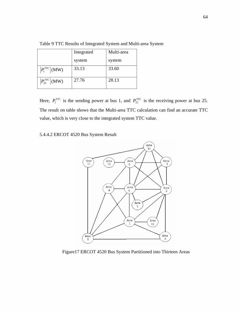
64
Table 9 TTC Results of Integrated System and Multi-area System
Integrated
system
Multi-area
system TTCP1 (MW) 33.13 33.60
TTCP25 (MW) 27.76 28.13
Here, TTCP1 is the sending power at bus 1, and TTCP25 is the receiving power at bus 25.
The result on table shows that the Multi-area TTC calculation can find an accurate TTC
value, which is very close to the integrated system TTC value.
5.4.4.2 ERCOT 4520 Bus System Result
Figure17 ERCOT 4520 Bus System Partitioned into Thirteen Areas

65
The base case of this system is ERCOT 4520 bus system data. The decomposition of the
system is shown in Figure 17. The objective is to find the TTC between 5026 (area 3)
and 5905 (area 11). The decomposition of the ERCOT system is shown in Fig. 17
In this part, three limiting cases will be studied; each case will not have voltage limit
violation but have one line flow limit violation at different area. DC PTDF as well as AC
PTDF matrix will be applied in TTC calculation at each case separately. The result is
listed in Table 10.
The result shows:
• The multi-area TTC result is very close to integrated TTC result.
• The more accurate PTDF the more accurate TTC result.
In order to generate the DC PTDF, the topology information of overall system is
necessary; but for AC PTDF, not only the topology information but also the power flow
information of current status (Jacobian matrix or load and injection information) of
overall system are necessary. The advantage of applying AC PTDF is accurate result, but
the price is more information exchange between area and central entity.
Table 10 TTC Results of Integrated System and Multi-area System of ERCOT 4520 Bus
System
Line
Limitation
Limitation
value
(MVA)
Integrated
TTC
(MW)
Multi-
Area TTC
with DC
PTDF
Multi-
Area TTC
with AC
PTDF
5901-5902
(area 11)
150 83.7 83.1 83.6
5025-5230
(area 3)
180 85.4 85.9 85.5
5502-5730
(area 10)
150 19.8 22.1 20.0

66
5.5 Conclusion
In this chapter a new method is presented, which has the hierarchical structure, to solve
the TTC problem of Multi-area power system. The proposed set-up is particularly
suitable for the deregulated power system with several areas where each area may solve
its own TTC based on DC PTDF matrix, and the central entity coordinate the result from
each area. There is no information exchange between each area, and limited information
exchange between areas and central entity. Simulation results on 30 and 4520 bus
system are shown to demonstrate the details of the proposed scheme.

67
CHAPTER VI
CONCLUSIONS
6.1 Summary
This dissertation addresses several important technical topics associated with the multi-
area power system operation. After the deregulation of the power systems, operators are
faced with the need to monitor and coordinate power transactions taking place over large
distances in different areas of the power systems and each area has its own control
center. The control areas are reluctant to share network and application data between
them. But it is necessry to have central entity to monitor and control the overall system,
so the overall system solutions (such as power flow, state estimation, total transfer
capability calculation, etc.) are needed. A new application scheme, which has a
hierarchical structure, is presented in the dissertation, and it is applied in the state
estimation and total transfer capability calculation. Following are the main achievements
of this dissertation:
• A new application scheme is designed to solve multi-area power system problem
by giving local area centers freedom for solving their own problems while the
central entity integrates their results. That is to say, in each area, the control
center keeps its own applications, and the central entity addresses the overall
system solution basing on the received results from each local area. As a result,
the information exchange between the areas is avoided.
• In state estimation, through proper decomposition of the system, the boundary
injection measurements can be used in the local area state estimator and
coordinator state estimator.
• In state estimation, the issue of bad data detection at area boundaries is
accomplished. The bad data can be detected and identified either by the local
state estimator or by the coordinator state estimator.
• In state estimation, synchronized phasor measurements are applied in the
coordinator state estimator. In case of low measurements redundancy at the area

68
boundaries, the phasor measurements can be helpful in improving the
redundancy and detecting bad data by the coordinator state;
• In total transfer capability calculation, the power transfer distribution factors
(PTDFs) are generated by the central entity and then are applied in the local TTC
calculation so that no information is exchanged between the areas in solving
local TTC problem.
6.2 Suggestions for Future Research
The work reported in this dissertation can be an important basis for future research
activities related to multi-area system operation. In general, future research directions
based on this dissertation are summarized below:
• In TTC calculation, the contingencies, such as line outage, may be considered in
the future research.
• Extend the multi-area solution scheme evaluate the Available Transfer Capabiltiy
(ATC) study, which involves other functions such as Capacity Benefit Margin
(CBM), Transfer Reliability Margin (TRM).
• Another posibility is to extend the same idea to other application functions, such
as voltage stability and transient stability calculations.

69
REFERENCES
[1] Promoting Wholesale Competition Through Open Access Non-discriminatory
Transmission Services by Public Utilities; Recovery of Stranded Costs by Public
Utilities and Transmitting Utilities. FERC. [Online]. Available:
http://www.ferc.gov/legal/ferc-regs/land-docs/order888.asp
[2] Open Access Same-Time Information System (formerly Real-Time Information
Networks) and Standards of Conduct. FERC. [Online]. Available:
http://www.ferc.gov/legal/ferc-regs/land-docs/order889.asp
[3] Final Rule, Regional Transmission Organization (RTO). FERC. [Online].
Available: http://www.ferc.gov/legal/ferc-regs/land-docs/RM99-2A.pdf
[4] G.B. Shrestha, K. Song, and L. Goel, “Strategic Self-dispatch Considering
Ramping Costs in Deregulated Power Markets”, IEEE Transactions on Power
Systems, vol. 19, pp. 1575–1581, Aug. 2004.
[5] X.H. Guan, F. Gao, and A.J. Svoboda, “Energy Delivery Capacity and Generation
Scheduling in the Deregulated Electric Power Market”, IEEE Transactions on
Power Systems, vol. 15, pp. 1275–1280, Nov. 2000.
[6] K. Lee, and R. Baldick, “Solving Three-player Games by the Matrix Approach
with Application to an Electric Power Market”, IEEE Transactions on Power
Systems, vol. 18, pp. 1573–1580, Nov. 2003.
[7] C. Silva, B.F. Wollenberg, and C.Z. Zheng, “Application of Mechanism Design to
Electric Power Markets”, IEEE Transactions on Power Systems, vol. 16, pp. 1–
8, Feb. 2001.
[8] C. Skoulidas, C. Vournas, and G. Papavassilopoulos, “Adaptive Game Modeling
of Deregulated Power Markets”, IEEE Power Engineering Review, vol. 22, pp.
42-45, Sept. 2002.
[9] R. Ragupathi, and T.K. Das, “A Stochastic Game Approach for Modeling
Wholesale Energy Bidding in Deregulated Power Markets”, IEEE Transactions on
Power Systems, vol. 19, pp. 849–856, May 2004.

70
[10] S.N. Singh, and A. K. David, “Towards Dynamic Security-constrained Congestion
Management in Open Power Market”, IEEE Power Engineering Review, vol. 20,
pp. 45-47, Aug. 2000.
[11] J. Douglas, ”Buying and Selling Power in the Age of Competition”, IEEE Power
Engineering Review, vol. 14, pp. 12-15, Oct. 1994.
[12] J. Zhong, E. Nobile, A. Bose, and K. Bhattacharya, “Localized Reactive Power
Markets Using the Concept of Voltage Control Areas”, IEEE Transactions on
Power Systems, vol. 19, pp. 1555–1561, Aug. 2004.
[13] P. Wang, and R. Billinton, “Reliability Assessment of a Restructured Power
System Considering the Reserve Agreements”, IEEE Transactions on Power
Systems, vol. 19, pp. 972–978, May 2004.
[14] A. Kumar, S.C. Srivastava, and S.N. Singh, “A Zonal Congestion Management
Approach Using Real and Reactive Power Rescheduling”, IEEE Transactions on
Power Systems, vol. 19, pp. 554–562, Feb. 2004.
[15] F. Albuyeh, and J. Kumar, “Decision Support Tools for Market Participants”,
IEEE Transactions on Power Systems, vol. 18, pp. 512–516, May 2004.
[16] R. Dahlgren, C.C. Liu, and J. Lawarree, “Risk Assessment in Energy Trading”,
IEEE Transactions on Power Systems, vol. 18, pp. 503–511, May 2004.
[17] A.F. Rahimi, and A.Y. Sheffrin, “Effective Market Monitoring in Deregulated
Electricity Markets”, IEEE Transactions on Power Systems, vol. 18, pp. 486–
493, May 2003.
[18] L. Battistelli, D. Lauria, and D. Proto, “Reactive Control in a Deregulated
Environment with Static VAR Compensators Improving Voltage Stability”, IEE
Proceedings on Generation, Transmission and Distribution, vol. 150, pp. 113-
18, Jan. 2003.
[19] N. Flatabo, G. Doorman, O.S. Grande, H. Randen, and I. Wangensteen,
“Experience with the Nord Pool Design and Implementation”, IEEE Transactions
on Power Systems, vol. 18, pp. 541–547, May 2003.
[20] C. Vazquez, M. Rivier, and I.J. Perez-Arriaga, “A Market Approach to Long-term

71
Security of Supply”, IEEE Transactions on Power Systems, vol. 17, pp. 349–
357, May 2004.
[21] D.T. Torre, J.W. Feltes, S.R. Gomez, and H.M. Merrill, “Deregulation,
Privatization, and Competition: Transmission Planning under Uncertainty”, IEEE
Transactions on Power Systems, vol. 14, pp. 460–465, May 1999.
[22] T.E. Dy-Liacco, “Modern Control Centers and Computer Networking”, Computer
Applications in Power, vol. 7, pp. 17-22, Oct. 1994.
[23] K.A. Clements, O.J. Denison, and R.J. Ringlee, “A Multi-area Approach to State
Estimation in Power System Networks”, Proc. IEEE/PES Summer Meeting, pp.
465-473, Jan. 1973.
[24] H. Kobayshi, S. Narita, and M.S.A.A. Hamman, “Model Coordination Method
Applied to Power System Control and Estimation Problems”, Presented at the
Proc. IFAC/IFIP 4th Int. Conf. on Digital Computer Appl. to Process Control, pp.
114-128, 1974.
[25] T. Van Cutsem, J.L. Horward, and M. Ribbens-Pavella, “A Two-level Static State
Estimator for Electric Power Systems”, IEEE Transactions on PAS, vol. PAS-100,
pp. 3722-3732, Aug. 1981.
[26] E. Mukai, “Report of Research Project 1764-1: Parallel Multiarea State
Estimation” Electric Power Research Institute , Jan. 1982.
[27] Y. Xiao, Y.H. Song, “Available Transfer Capability (ATC) Evaluation by
Stochastic Programming”. IEEE Power Engineering Review, vol. 20, pp. 50-52,
Sept. 2000.
[28] G.C. Ejebe, J. Tong, J.G. Waight, J.G. Frame, X. Wang, and W.F. Tinney,
“Available Transfer Capability Calculations”, IEEE Transactions on Power
Systems, vol. 13, pp. 1521–1527, Nov. 1998.
[29] R.F. Chang, C.Y. Tsai, C.L. Su, and C.N. Lu, “Method for Computing Probability
Distributions of Available Transfer Capability”, IEE Proceedings on Generation,
Transmission and Distribution, vol. 149, pp. 427-431 July 2002.
[30] B. Stott, “Review of Load Flow Calculation Methods”, Proc, 1974 IEEE-, vol. 62,

72
pp. 916-929, Aug. 1974.
[31] G. Cohen, and D.L. Zhu, “Decomposition Coordination Methods in Large Scale
Optimization Problems: the Non-differentiable Case and the Use of Augmented
Lagrangians”, Adv. Large Scale Syst., vol. 1, pp. 203-266, 1984
[32] M. Shaaban, W. Li, H. Liu, Z. Yan, Y.X. Ni, and F.F. Wu, “ATC Calculation with
Steady-state Security Constraints Using Benders Decomposition”, IEE
Proceedings on Generation, Transmission and Distribution, vol. 150, pp. 611-615,
Sept. 2003.
[33] A. Monticelli, State Estimation in Electric Power Systems: a Generalized
Approach, Boston: Kluwer Academic Publishers, 1999.
[34] A. Monticelli, and F.F. Wu, “Network Observability: Identification of Observable
Islands and Measurement Placement”, IEEE Transactions on PAS, vol. PAS-104,
pp. 1035-1041, May 1985.
[35] A. Monticelli, and F.F. Wu, “Network Observability: Theory”, IEEE Transactions
on PAS, vol. PAS-104, pp. 1042-1048, May 1985.
[36] G.R. Krumpholz, K.A. Clements, and P.W. Davis, “Power System Observability:
a Practical Algorithm Using Network Topology”, IEEE Transactions on PAS, vol.
PAS-99, pp. 1534-1542, July/Aug. 1980.
[37] K.A. Clements, G.R. Krumpholz, and P.W. Davis, “Power System State
Estimation with Measurement Deficiency: an Observability/Measurement
Placement Algorithm”, IEEE Transactions on PAS, vol. 102, pp. 2012-2020, July
1983.
[38] K.A. Clements, G.R. Krumpholz, and P.W. Davis, “Power System State
Estimation with Measurement Deficiency: an Algorithm that Determines the
Maximal Observable Subnetwork”, IEEE Transactions on PAS, vol. 101, pp.
3044-3052, July 1982.
[39] K.A. Clements, G.R. Krumpholz, and P.W. Davis, “Power System State
Estimation with Measurement Deficiency: an Algorithm Using Network
Topology”, IEEE Transactions on PAS, vol. 101, pp. 1779-1787, July 1982.

73
[40] A. Monticelli, and A. Garcia, “Reliable Bad Data Processing for Real-time State
Estimation”, IEEE Transactions on PAS, vol. PAS-102, pp. 1126-1139, July 1983.
[41] E. Handschin, F.C. Schweppe, J. Kohlas, and A. Fiechter, “Bad Data Analysis for
Power System State Estimation”, IEEE Transactions on PAS, vol. PAS-94, pp.
329-337, July 1975.
[42] A.G. Phadke, “Sychronized Phasor Measurement”, Computer Applications in
Power, vol. 6 , pp. 10-15, April 1993.
[43] J.S. Thorp, A.G. Phadke, S.H. Horowitz, and M.M. Begovic, “Some Applications
of Phasor Measurements to Adaptive Protection”, IEEE Transactions on Power
Systems, vol. 3, pp. 791–798, May 1998.
[44] B. Milosevic, and M Begovic, “Voltage-stability Protection and Control Using a
Wide-area Network of Phasor Measurements”, IEEE Transactions on Power
Systems, vol. 18, pp. 121–127, Feb. 2003.
[45] A.G. Phadke, B. Pickett, M. Adamiak, M. Begovic, G. Benmouyal, R.O. Burnett,
T.W. Cease, J. Goossens, D.J. Hansen, M. Kezunovic, L.L. Mankoff, P.G.
McLaren, G. Michel, R.J. Murphy, J. Nordstrom, M.S. Sachdev, H.S. Smith, J.S.
Thorp, M. Trotignon, T.C. Wang, and M.A. Xavier, “Synchronized Sampling and
Phasor Measurements for Relaying and Control”, IEEE
Transactions on Power Delivery, vol. 9 , pp. 442-452, Jan. 1994.
[46] R.O. Burnett, J. Butts, T.W. Cease, V. Centeno, G. Michel, R.J. Murphy, and A.G.
Phadke, “Synchronized Phasor Measurements of a Power System Event”, IEEE
Transactions on Power Systems, vol. 9, pp. 1643–1650, Aug. 1994.
[47] J.S. Thorp, A.G. Phadke, and K.J. Karimi, “Real Time Voltage-Phasor
Measurements for Static State Estimation”. IEEE Transactions on PAS, vol. PAS-
104, pp. 1779-1787, Aug. 1985.
[48] A.G. Phadke, J.S. Thorp, and K.J. Karimi, “State Estimation with Phasor
Measurements”. IEEE Transactions on PAS, vol. PAS-105, pp. 1231-1237, Aug.
1986.
[49] R. Zivanovic, and C. Cairns, “Implementation of PMU Technology in State

74
Estimation: an Overview”. IEEE Proceedings on AFRICON 4th, vol. 2, pp. 1006-
1011, July, 1996.
[50] L. Zhao, and A. Abur, “A Two-Level State Estimator for Multi-ISO Operation”,
Proceedings of the Thirty-fifth Annual North American Power Symposium. [CD-
ROM]. Rolla, Missouri, 2003.
[51] Power Systems Test Case, Electrical Engineering Department, University of
Washington. [Online]. Available: http://www.ee.washington.edu/research/pstca/
[52] A. Abur, and M.K. Çelik, “Multi-Area Linear Programming State Estimator Using
Dantzig-Wolfe Decomposition”, Proceedings Tenth Power Systems Computations
Conference, Graz, Austria, August 1990, pp.1038-1044.
[53] Transmission Transfer Capability Task Force, “Transmission Transfer
Capability”, North American Reliability Council, Princeton, New Jersey, 1995.
[54] Transmission Transfer Capability Task Force, “Available Transmission Capability
Definitions and Determination”, North American Reliability Council, Princeton,
New Jersey, 1996.
[55] I. Dobson, S. Greene, R. Rajaraman, C.L. Demarco, F.L. Alvarado, M. Glavic, J.
Zhang, and R. Zimmerman, Electrical Power Transfer Capability: Concepts,
Applications, Sensitivity, Uncertainty. Power Systems Engineering Research
Center. [Online]. Available:
http://www.pserc.cornell.edu/tcc/tutorial/TCC_Tutorial.pdf
[56] V. Ajjarapu, and C. Christy, “The Continuation Power Flow: a Tool for Steady
State Voltage Stability Analysis”, IEEE Transactions on Power Systems, vol. 7,
pp. 416–423, Feb. 1992.
[57] C.A. Canizares, and F.L. Alvarado, “Point of Collapse and Continuation Methods
for Large AC/DC Systems”, IEEE Transactions on Power Systems, vol. 7, pp. 1–
8, Feb. 1993.
[58] H.D. Chiang, A. Flueck, K.S. Shah, and N. Balu, “CPFLOW: A Practical Tool for
Tracing Power System Steady-state Stationary Behavior Due to Load and
Generation Variations”, IEEE Transactions on Power Systems, vol. 10, pp. 623–

75
634, May. 1995.
[59] S. Hao, G.A. Angelidis, H. Singh, and A.D. Papalexopoulos, ”Consumer Payment
Minimizaion in Power Pool Auction”, IEEE Transactions on Power Systems, vol.
13., pp. 986-991, Aug. 1998.
[60] M.D. Ilic, J.R. Lacalle-Melero, F. Nishinmura, W. Schenler, D. Shirmohammadi,
A. Crough, and A. Catelli, “Short-term Economic Energy Management in a
Competetitive Utility Enviroment”, IEEE Transactions on Power Systems, vol. 8,
pp. 198-206, Feb. 1993.
[61] H. Singh, S. Hao, and A. Papalexopoulos, “Transmission Congestion Management
in Competitive Electricity Markets”, IEEE Transactions on Power Systems, vol.
13, pp.672-680, May 1998.
[62] A. Papalexopoulos, “Challenges to On-line Optimal Power Flow Implementation”,
IEEE Transactions on Power Systems, vol. 12, pp 449-451, Feb. 1997.
[63] M. Pavella, D. Ruiz-Vega, J. Giri, and R. Avila-Rosales, “An Integrated Scheme
for On-line Static and Transient Stability Constrained ATC Calculations”, Proc.
1999 IEEE/PES Summer Meeting, vol. 1, pp. 273-276, July 1999.
[64] X. Wang and Y.H. Song, “Advanced Real-time Congestion Management through
Both Pool Balancing Market and Bilateral Market”, IEEE Power Engineering
Review, vol. 20, pp. 47-49, Feb. 2000.
[65] C.N. Yu, and M.D. Ilic, “An Algorithm for Implementing Transmission Rights in
a Competitive Power Industry”, Proc. 2000 IEEE/PES Winter Meeting, vol. 3, pp.
1708-1714, Jan. 2000.
[66] M.H. Gravener, and C. Nwankpa, “Available Transfer Capability and First Order
Sensitivity”, IEEE Transactions on Power Systems, vol. 14, pp. 512–518, May
1999.
[67] Y. Ou, and C. Singh, “Improvement of Total Transfer Capability Using TCSC and
SVC”, Proc. 2001 IEEE/PES Summer Meeting, vol. 2, pp. 944-948, July 2001.
[68] A. Fradi, S. Brignone, and B.F. Wollenberg, “Calcualtion of Energy Transaction
Allocation Factors”, IEEE Transactions on Power Systems, vol. 16, pp. 266–

76
272, May 2001.
[69] R. Christie, B.F. Wollenberg, and I. Wangstein, “Transmission Management in
Deregulated Environment”, IEEE Proc., vol. 88, pp. 170-195, Feb. 2000.
[70] M. Shaaban, Y.X. Ni, H.W. Dai, and F.F. Wu, “Considerations in Calculating
Total Transfer Capability”, in Proc. Intl. Conference on POWERCON, Beijing,
Aug. 1998, pp. 1356-1360.

77
APPENDIX A
DATA OF THE IEEE30-BUS SYSTEM
08/20/93 UW ARCHIVE 100.0 1961 W IEEE 30 Bus Test Case BUS DATA FOLLOWS 30 ITEMS 1 Glen Lyn 132 1 1 3 1.060 0.0 0.0 0.0 260.2 -16.1 132.0 1.060 0.0 0.0 0.0 0.0 0 2 Claytor 132 1 1 2 1.043 -5.48 21.7 12.7 40.0 50.0 132.0 1.045 50.0 -40.0 0.0 0.0 0 3 Kumis 132 1 1 0 1.021 -7.96 2.4 1.2 0.0 0.0 132.0 0.0 0.0 0.0 0.0 0.0 0 4 Hancock 132 1 1 0 1.012 -9.62 7.6 1.6 0.0 0.0 132.0 0.0 0.0 0.0 0.0 0.0 0 5 Fieldale 132 1 1 2 1.010 -14.37 94.2 19.0 0.0 37.0 132.0 1.010 40.0 -40.0 0.0 0.0 0 6 Roanoke 132 1 1 0 1.010 -11.34 0.0 0.0 0.0 0.0 132.0 0.0 0.0 0.0 0.0 0.0 0 7 Blaine 132 1 1 0 1.002 -13.12 22.8 10.9 0.0 0.0 132.0 0.0 0.0 0.0 0.0 0.0 0 8 Reusens 132 1 1 2 1.010 -12.10 30.0 30.0 0.0 37.3 132.0 1.010 40.0 -10.0 0.0 0.0 0 9 Roanoke 1.0 1 1 0 1.051 -14.38 0.0 0.0 0.0 0.0 1.0 0.0 0.0 0.0 0.0 0.0 0 10 Roanoke 33 1 1 0 1.045 -15.97 5.8 2.0 0.0 0.0 33.0 0.0 0.0 0.0 0.0 0.19 0 11 Roanoke 11 1 1 2 1.082 -14.39 0.0 0.0 0.0 16.2 11.0 1.082 24.0 -6.0 0.0 0.0 0 12 Hancock 33 1 1 0 1.057 -15.24 11.2 7.5 0.0 0.0 33.0 0.0 0.0 0.0 0.0 0.0 0 13 Hancock 11 1 1 2 1.071 -15.24 0.0 0.0 0.0 10.6 11.0 1.071 24.0 -6.0 0.0 0.0 0 14 Bus 14 33 1 1 0 1.042 -16.13 6.2 1.6 0.0 0.0 33.0 0.0 0.0 0.0 0.0 0.0 0 15 Bus 15 33 1 1 0 1.038 -16.22 8.2 2.5 0.0 0.0 33.0 0.0 0.0 0.0 0.0 0.0 0 16 Bus 16 33 1 1 0 1.045 -15.83 3.5 1.8 0.0 0.0 33.0 0.0 0.0 0.0 0.0 0.0 0 17 Bus 17 33 1 1 0 1.040 -16.14 9.0 5.8 0.0 0.0 33.0 0.0 0.0 0.0 0.0 0.0 0 18 Bus 18 33 1 1 0 1.028 -16.82 3.2 0.9 0.0 0.0 33.0 0.0 0.0 0.0 0.0 0.0 0 19 Bus 19 33 1 1 0 1.026 -17.00 9.5 3.4 0.0 0.0 33.0 0.0 0.0 0.0 0.0 0.0 0 20 Bus 20 33 1 1 0 1.030 -16.80 2.2 0.7 0.0 0.0 33.0 0.0 0.0 0.0 0.0 0.0 0 21 Bus 21 33 1 1 0 1.033 -16.42 17.5 11.2 0.0 0.0 33.0 0.0 0.0 0.0 0.0 0.0 0 22 Bus 22 33 1 1 0 1.033 -16.41 0.0 0.0 0.0 0.0 33.0 0.0 0.0 0.0 0.0 0.0 0
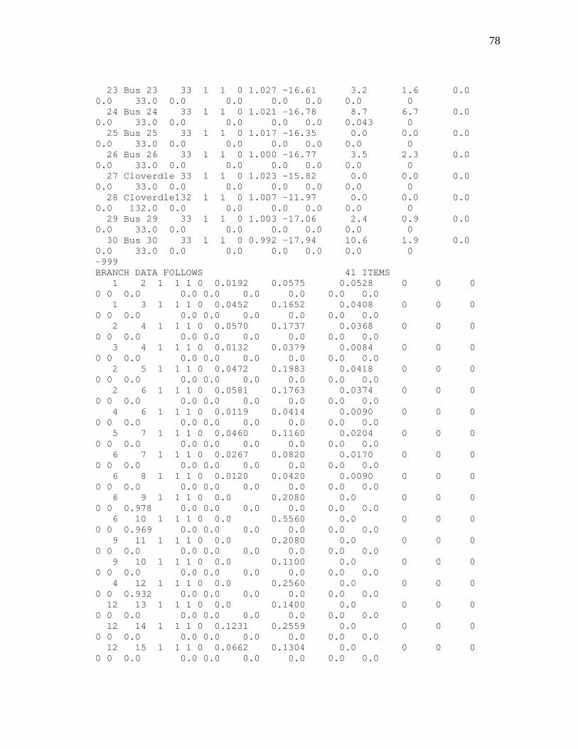
78
23 Bus 23 33 1 1 0 1.027 -16.61 3.2 1.6 0.0 0.0 33.0 0.0 0.0 0.0 0.0 0.0 0 24 Bus 24 33 1 1 0 1.021 -16.78 8.7 6.7 0.0 0.0 33.0 0.0 0.0 0.0 0.0 0.043 0 25 Bus 25 33 1 1 0 1.017 -16.35 0.0 0.0 0.0 0.0 33.0 0.0 0.0 0.0 0.0 0.0 0 26 Bus 26 33 1 1 0 1.000 -16.77 3.5 2.3 0.0 0.0 33.0 0.0 0.0 0.0 0.0 0.0 0 27 Cloverdle 33 1 1 0 1.023 -15.82 0.0 0.0 0.0 0.0 33.0 0.0 0.0 0.0 0.0 0.0 0 28 Cloverdle132 1 1 0 1.007 -11.97 0.0 0.0 0.0 0.0 132.0 0.0 0.0 0.0 0.0 0.0 0 29 Bus 29 33 1 1 0 1.003 -17.06 2.4 0.9 0.0 0.0 33.0 0.0 0.0 0.0 0.0 0.0 0 30 Bus 30 33 1 1 0 0.992 -17.94 10.6 1.9 0.0 0.0 33.0 0.0 0.0 0.0 0.0 0.0 0 -999 BRANCH DATA FOLLOWS 41 ITEMS 1 2 1 1 1 0 0.0192 0.0575 0.0528 0 0 0 0 0 0.0 0.0 0.0 0.0 0.0 0.0 0.0 1 3 1 1 1 0 0.0452 0.1652 0.0408 0 0 0 0 0 0.0 0.0 0.0 0.0 0.0 0.0 0.0 2 4 1 1 1 0 0.0570 0.1737 0.0368 0 0 0 0 0 0.0 0.0 0.0 0.0 0.0 0.0 0.0 3 4 1 1 1 0 0.0132 0.0379 0.0084 0 0 0 0 0 0.0 0.0 0.0 0.0 0.0 0.0 0.0 2 5 1 1 1 0 0.0472 0.1983 0.0418 0 0 0 0 0 0.0 0.0 0.0 0.0 0.0 0.0 0.0 2 6 1 1 1 0 0.0581 0.1763 0.0374 0 0 0 0 0 0.0 0.0 0.0 0.0 0.0 0.0 0.0 4 6 1 1 1 0 0.0119 0.0414 0.0090 0 0 0 0 0 0.0 0.0 0.0 0.0 0.0 0.0 0.0 5 7 1 1 1 0 0.0460 0.1160 0.0204 0 0 0 0 0 0.0 0.0 0.0 0.0 0.0 0.0 0.0 6 7 1 1 1 0 0.0267 0.0820 0.0170 0 0 0 0 0 0.0 0.0 0.0 0.0 0.0 0.0 0.0 6 8 1 1 1 0 0.0120 0.0420 0.0090 0 0 0 0 0 0.0 0.0 0.0 0.0 0.0 0.0 0.0 6 9 1 1 1 0 0.0 0.2080 0.0 0 0 0 0 0 0.978 0.0 0.0 0.0 0.0 0.0 0.0 6 10 1 1 1 0 0.0 0.5560 0.0 0 0 0 0 0 0.969 0.0 0.0 0.0 0.0 0.0 0.0 9 11 1 1 1 0 0.0 0.2080 0.0 0 0 0 0 0 0.0 0.0 0.0 0.0 0.0 0.0 0.0 9 10 1 1 1 0 0.0 0.1100 0.0 0 0 0 0 0 0.0 0.0 0.0 0.0 0.0 0.0 0.0 4 12 1 1 1 0 0.0 0.2560 0.0 0 0 0 0 0 0.932 0.0 0.0 0.0 0.0 0.0 0.0 12 13 1 1 1 0 0.0 0.1400 0.0 0 0 0 0 0 0.0 0.0 0.0 0.0 0.0 0.0 0.0 12 14 1 1 1 0 0.1231 0.2559 0.0 0 0 0 0 0 0.0 0.0 0.0 0.0 0.0 0.0 0.0 12 15 1 1 1 0 0.0662 0.1304 0.0 0 0 0 0 0 0.0 0.0 0.0 0.0 0.0 0.0 0.0

79
12 16 1 1 1 0 0.0945 0.1987 0.0 0 0 0 0 0 0.0 0.0 0.0 0.0 0.0 0.0 0.0 14 15 1 1 1 0 0.2210 0.1997 0.0 0 0 0 0 0 0.0 0.0 0.0 0.0 0.0 0.0 0.0 16 17 1 1 1 0 0.0524 0.1923 0.0 0 0 0 0 0 0.0 0.0 0.0 0.0 0.0 0.0 0.0 15 18 1 1 1 0 0.1073 0.2185 0.0 0 0 0 0 0 0.0 0.0 0.0 0.0 0.0 0.0 0.0 18 19 1 1 1 0 0.0639 0.1292 0.0 0 0 0 0 0 0.0 0.0 0.0 0.0 0.0 0.0 0.0 19 20 1 1 1 0 0.0340 0.0680 0.0 0 0 0 0 0 0.0 0.0 0.0 0.0 0.0 0.0 0.0 10 20 1 1 1 0 0.0936 0.2090 0.0 0 0 0 0 0 0.0 0.0 0.0 0.0 0.0 0.0 0.0 10 17 1 1 1 0 0.0324 0.0845 0.0 0 0 0 0 0 0.0 0.0 0.0 0.0 0.0 0.0 0.0 10 21 1 1 1 0 0.0348 0.0749 0.0 0 0 0 0 0 0.0 0.0 0.0 0.0 0.0 0.0 0.0 10 22 1 1 1 0 0.0727 0.1499 0.0 0 0 0 0 0 0.0 0.0 0.0 0.0 0.0 0.0 0.0 21 22 1 1 1 0 0.0116 0.0236 0.0 0 0 0 0 0 0.0 0.0 0.0 0.0 0.0 0.0 0.0 15 23 1 1 1 0 0.1000 0.2020 0.0 0 0 0 0 0 0.0 0.0 0.0 0.0 0.0 0.0 0.0 22 24 1 1 1 0 0.1150 0.1790 0.0 0 0 0 0 0 0.0 0.0 0.0 0.0 0.0 0.0 0.0 23 24 1 1 1 0 0.1320 0.2700 0.0 0 0 0 0 0 0.0 0.0 0.0 0.0 0.0 0.0 0.0 24 25 1 1 1 0 0.1885 0.3292 0.0 0 0 0 0 0 0.0 0.0 0.0 0.0 0.0 0.0 0.0 25 26 1 1 1 0 0.2544 0.3800 0.0 0 0 0 0 0 0.0 0.0 0.0 0.0 0.0 0.0 0.0 25 27 1 1 1 0 0.1093 0.2087 0.0 0 0 0 0 0 0.0 0.0 0.0 0.0 0.0 0.0 0.0 28 27 1 1 1 0 0.0 0.3960 0.0 0 0 0 0 0 0.968 0.0 0.0 0.0 0.0 0.0 0.0 27 29 1 1 1 0 0.2198 0.4153 0.0 0 0 0 0 0 0.0 0.0 0.0 0.0 0.0 0.0 0.0 27 30 1 1 1 0 0.3202 0.6027 0.0 0 0 0 0 0 0.0 0.0 0.0 0.0 0.0 0.0 0.0 29 30 1 1 1 0 0.2399 0.4533 0.0 0 0 0 0 0 0.0 0.0 0.0 0.0 0.0 0.0 0.0 8 28 1 1 1 0 0.0636 0.2000 0.0428 0 0 0 0 0 0.0 0.0 0.0 0.0 0.0 0.0 0.0 6 28 1 1 1 0 0.0169 0.0599 0.0130 0 0 0 0 0 0.0 0.0 0.0 0.0 0.0 0.0 0.0 -999 LOSS ZONES FOLLOWS 1 ITEMS 1 IEEE 30 BUS -99 INTERCHANGE DATA FOLLOWS 1 ITEMS -9 1 2 Claytor 132 0.0 999.99 IEEE30 IEEE 30 Bus Test Case TIE LINES FOLLOWS 0 ITEMS

80
-999 END OF DATA
Figure. 18 IEEE 30 Bus System Diagram

81
APPENDIX B
DATA OF THE IEEE118-BUS SYSTEM
08/25/93 UW ARCHIVE 100.0 1961 W IEEE 118 Bus Test Case BUS DATA FOLLOWS 57 ITEMS 1 Riversde V2 1 1 2 0.955 10.67 51.0 27.0 0.0 0.0 0.0 0.955 15.0 -5.0 0.0 0.0 0 2 Pokagon V2 1 1 0 0.971 11.22 20.0 9.0 0.0 0.0 0.0 0.0 0.0 0.0 0.0 0.0 0 3 HickryCk V2 1 1 0 0.968 11.56 39.0 10.0 0.0 0.0 0.0 0.0 0.0 0.0 0.0 0.0 0 4 NwCarlsl V2 1 1 2 0.998 15.28 30.0 12.0 -9.0 0.0 0.0 0.998 300.0 -300.0 0.0 0.0 0 5 Olive V2 1 1 0 1.002 15.73 0.0 0.0 0.0 0.0 0.0 0.0 0.0 0.0 0.0 -0.40 0 6 Kankakee V2 1 1 2 0.990 13.00 52.0 22.0 0.0 0.0 0.0 0.990 50.0 -13.0 0.0 0.0 0 7 JacksnRd V2 1 1 0 0.989 12.56 19.0 2.0 0.0 0.0 0.0 0.0 0.0 0.0 0.0 0.0 0 8 Olive V1 1 1 2 1.015 20.77 0.0 0.0 -28.0 0.0 0.0 1.015 300.0 -300.0 0.0 0.0 0 9 Bequine V1 1 1 0 1.043 28.02 0.0 0.0 0.0 0.0 0.0 0.0 0.0 0.0 0.0 0.0 0 10 Breed V1 1 1 2 1.050 35.61 0.0 0.0 450.0 0.0 0.0 1.050 200.0 -147.0 0.0 0.0 0 11 SouthBnd V2 1 1 0 0.985 12.72 70.0 23.0 0.0 0.0 0.0 0.0 0.0 0.0 0.0 0.0 0 12 TwinBrch V2 1 1 2 0.990 12.20 47.0 10.0 85.0 0.0 0.0 0.990 120.0 -35.0 0.0 0.0 0 13 Concord V2 1 1 0 0.968 11.35 34.0 16.0 0.0 0.0 0.0 0.0 0.0 0.0 0.0 0.0 0 14 GoshenJt V2 1 1 0 0.984 11.50 14.0 1.0 0.0 0.0 0.0 0.0 0.0 0.0 0.0 0.0 0 15 FtWayne V2 1 1 2 0.970 11.23 90.0 30.0 0.0 0.0 0.0 0.970 30.0 -10.0 0.0 0.0 0 16 N. E. V2 1 1 0 0.984 11.91 25.0 10.0 0.0 0.0 0.0 0.0 0.0 0.0 0.0 0.0 0 17 Sorenson V2 1 1 0 0.995 13.74 11.0 3.0 0.0 0.0 0.0 0.0 0.0 0.0 0.0 0.0 0 18 McKinley V2 1 1 2 0.973 11.53 60.0 34.0 0.0 0.0 0.0 0.973 50.0 -16.0 0.0 0.0 0 19 Lincoln V2 1 1 2 0.963 11.05 45.0 25.0 0.0 0.0 0.0 0.962 24.0 -8.0 0.0 0.0 0 20 Adams V2 1 1 0 0.958 11.93 18.0 3.0 0.0 0.0 0.0 0.0 0.0 0.0 0.0 0.0 0 21 Jay V2 1 1 0 0.959 13.52 14.0 8.0 0.0 0.0 0.0 0.0 0.0 0.0 0.0 0.0 0 22 Randolph V2 1 1 0 0.970 16.08 10.0 5.0 0.0 0.0 0.0 0.0 0.0 0.0 0.0 0.0 0

82
23 CollCrnr V2 1 1 0 1.000 21.00 7.0 3.0 0.0 0.0 0.0 0.0 0.0 0.0 0.0 0.0 0 24 Trenton V2 1 1 2 0.992 20.89 0.0 0.0 -13.0 0.0 0.0 0.992 300.0 -300.0 0.0 0.0 0 25 TannrsCk V2 1 1 2 1.050 27.93 0.0 0.0 220.0 0.0 0.0 1.050 140.0 -47.0 0.0 0.0 0 26 TannrsCk V1 1 1 2 1.015 29.71 0.0 0.0 314.0 0.0 0.0 1.015 1000.0 -1000.0 0.0 0.0 0 27 Madison V2 1 1 2 0.968 15.35 62.0 13.0 -9.0 0.0 0.0 0.968 300.0 -300.0 0.0 0.0 0 28 Mullin V2 1 1 0 0.962 13.62 17.0 7.0 0.0 0.0 0.0 0.0 0.0 0.0 0.0 0.0 0 29 Grant V2 1 1 0 0.963 12.63 24.0 4.0 0.0 0.0 0.0 0.0 0.0 0.0 0.0 0.0 0 30 Sorenson V1 1 1 0 0.968 18.79 0.0 0.0 0.0 0.0 0.0 0.0 0.0 0.0 0.0 0.0 0 31 DeerCrk V2 1 1 2 0.967 12.75 43.0 27.0 7.0 0.0 0.0 0.967 300.0 -300.0 0.0 0.0 0 32 Delaware V2 1 1 2 0.964 14.80 59.0 23.0 0.0 0.0 0.0 0.963 42.0 -14.0 0.0 0.0 0 33 Haviland V2 1 1 0 0.972 10.63 23.0 9.0 0.0 0.0 0.0 0.0 0.0 0.0 0.0 0.0 0 34 Rockhill V2 1 1 2 0.986 11.30 59.0 26.0 0.0 0.0 0.0 0.984 24.0 -8.0 0.0 0.14 0 35 WestLima V2 1 1 0 0.981 10.87 33.0 9.0 0.0 0.0 0.0 0.0 0.0 0.0 0.0 0.0 0 36 Sterling V2 1 1 2 0.980 10.87 31.0 17.0 0.0 0.0 0.0 0.980 24.0 -8.0 0.0 0.0 0 37 EastLima V2 1 1 0 0.992 11.77 0.0 0.0 0.0 0.0 0.0 0.0 0.0 0.0 0.0 -0.25 0 38 EastLima V1 1 1 0 0.962 16.91 0.0 0.0 0.0 0.0 0.0 0.0 0.0 0.0 0.0 0.0 0 39 NwLibrty V2 1 1 0 0.970 8.41 27.0 11.0 0.0 0.0 0.0 0.0 0.0 0.0 0.0 0.0 0 40 West End V2 1 1 2 0.970 7.35 20.0 23.0 -46.0 0.0 0.0 0.970 300.0 -300.0 0.0 0.0 0 41 S.Tiffin V2 1 1 0 0.967 6.92 37.0 10.0 0.0 0.0 0.0 0.0 0.0 0.0 0.0 0.0 0 42 Howard V2 1 1 2 0.985 8.53 37.0 23.0 -59.0 0.0 0.0 0.985 300.0 -300.0 0.0 0.0 0 43 S.Kenton V2 1 1 0 0.978 11.28 18.0 7.0 0.0 0.0 0.0 0.0 0.0 0.0 0.0 0.0 0 44 WMVernon V2 1 1 0 0.985 13.82 16.0 8.0 0.0 0.0 0.0 0.0 0.0 0.0 0.0 0.10 0 45 N.Newark V2 1 1 0 0.987 15.67 53.0 22.0 0.0 0.0 0.0 0.0 0.0 0.0 0.0 0.10 0 46 W.Lancst V2 1 1 2 1.005 18.49 28.0 10.0 19.0 0.0 0.0 1.005 100.0 -100.0 0.0 0.10 0 47 Crooksvl V2 1 1 0 1.017 20.73 34.0 0.0 0.0 0.0 0.0 0.0 0.0 0.0 0.0 0.0 0 48 Zanesvll V2 1 1 0 1.021 19.93 20.0 11.0 0.0 0.0 0.0 0.0 0.0 0.0 0.0 0.15 0 49 Philo V2 1 1 2 1.025 20.94 87.0 30.0 204.0 0.0 0.0 1.025 210.0 -85.0 0.0 0.0 0

83
50 WCambrdg V2 1 1 0 1.001 18.90 17.0 4.0 0.0 0.0 0.0 0.0 0.0 0.0 0.0 0.0 0 51 Newcmrst V2 1 1 0 0.967 16.28 17.0 8.0 0.0 0.0 0.0 0.0 0.0 0.0 0.0 0.0 0 52 SCoshoct V2 1 1 0 0.957 15.32 18.0 5.0 0.0 0.0 0.0 0.0 0.0 0.0 0.0 0.0 0 53 Wooster V2 1 1 0 0.946 14.35 23.0 11.0 0.0 0.0 0.0 0.0 0.0 0.0 0.0 0.0 0 54 Torrey V2 1 1 2 0.955 15.26 113.0 32.0 48.0 0.0 0.0 0.955 300.0 -300.0 0.0 0.0 0 55 Wagenhls V2 1 1 2 0.952 14.97 63.0 22.0 0.0 0.0 0.0 0.952 23.0 -8.0 0.0 0.0 0 56 Sunnysde V2 1 1 2 0.954 15.16 84.0 18.0 0.0 0.0 0.0 0.954 15.0 -8.0 0.0 0.0 0 57 WNwPhil1 V2 1 1 0 0.971 16.36 12.0 3.0 0.0 0.0 0.0 0.0 0.0 0.0 0.0 0.0 0 58 WNwPhil2 V2 1 1 0 0.959 15.51 12.0 3.0 0.0 0.0 0.0 0.0 0.0 0.0 0.0 0.0 0 59 Tidd V2 1 1 2 0.985 19.37 277.0 113.0 155.0 0.0 0.0 0.985 180.0 -60.0 0.0 0.0 0 60 SWKammer V2 1 1 0 0.993 23.15 78.0 3.0 0.0 0.0 0.0 0.0 0.0 0.0 0.0 0.0 0 61 W.Kammer V2 1 1 2 0.995 24.04 0.0 0.0 160.0 0.0 0.0 0.995 300.0 -100.0 0.0 0.0 0 62 Natrium V2 1 1 2 0.998 23.43 77.0 14.0 0.0 0.0 0.0 0.998 20.0 -20.0 0.0 0.0 0 63 Tidd V1 1 1 0 0.969 22.75 0.0 0.0 0.0 0.0 0.0 0.0 0.0 0.0 0.0 0.0 0 64 Kammer V1 1 1 0 0.984 24.52 0.0 0.0 0.0 0.0 0.0 0.0 0.0 0.0 0.0 0.0 0 65 Muskngum V1 1 1 2 1.005 27.65 0.0 0.0 391.0 0.0 0.0 1.005 200.0 -67.0 0.0 0.0 0 66 Muskngum V2 1 1 2 1.050 27.48 39.0 18.0 392.0 0.0 0.0 1.050 200.0 -67.0 0.0 0.0 0 67 Summerfl V2 1 1 0 1.020 24.84 28.0 7.0 0.0 0.0 0.0 0.0 0.0 0.0 0.0 0.0 0 68 Sporn V1 1 1 0 1.003 27.55 0.0 0.0 0.0 0.0 0.0 0.0 0.0 0.0 0.0 0.0 0 69 Sporn V2 1 1 3 1.035 30.00 0.0 0.0 516.4 0.0 0.0 1.035 300.0 -300.0 0.0 0.0 0 70 Portsmth V2 1 1 2 0.984 22.58 66.0 20.0 0.0 0.0 0.0 0.984 32.0 -10.0 0.0 0.0 0 71 NPortsmt V2 1 1 0 0.987 22.15 0.0 0.0 0.0 0.0 0.0 0.0 0.0 0.0 0.0 0.0 0 72 Hillsbro V2 1 1 2 0.980 20.98 0.0 0.0 -12.0 0.0 0.0 0.980 100.0 -100.0 0.0 0.0 0 73 Sargents V2 1 1 2 0.991 21.94 0.0 0.0 -6.0 0.0 0.0 0.991 100.0 -100.0 0.0 0.0 0 74 Bellefnt V2 1 1 2 0.958 21.64 68.0 27.0 0.0 0.0 0.0 0.958 9.0 -6.0 0.0 0.12 0 75 SthPoint V2 1 1 0 0.967 22.91 47.0 11.0 0.0 0.0 0.0 0.0 0.0 0.0 0.0 0.0 0 76 Darrah V2 1 1 2 0.943 21.77 68.0 36.0 0.0 0.0 0.0 0.943 23.0 -8.0 0.0 0.0 0

84
77 Turner V2 1 1 2 1.006 26.72 61.0 28.0 0.0 0.0 0.0 1.006 70.0 -20.0 0.0 0.0 0 78 Chemical V2 1 1 0 1.003 26.42 71.0 26.0 0.0 0.0 0.0 0.0 0.0 0.0 0.0 0.0 0 79 CapitlHl V2 1 1 0 1.009 26.72 39.0 32.0 0.0 0.0 0.0 0.0 0.0 0.0 0.0 0.20 0 80 CabinCrk V2 1 1 2 1.040 28.96 130.0 26.0 477.0 0.0 0.0 1.040 280.0 -165.0 0.0 0.0 0 81 Kanawha V1 1 1 0 0.997 28.10 0.0 0.0 0.0 0.0 0.0 0.0 0.0 0.0 0.0 0.0 0 82 Logan V2 1 1 0 0.989 27.24 54.0 27.0 0.0 0.0 0.0 0.0 0.0 0.0 0.0 0.20 0 83 Sprigg V2 1 1 0 0.985 28.42 20.0 10.0 0.0 0.0 0.0 0.0 0.0 0.0 0.0 0.10 0 84 BetsyLne V2 1 1 0 0.980 30.95 11.0 7.0 0.0 0.0 0.0 0.0 0.0 0.0 0.0 0.0 0 85 BeaverCk V2 1 1 2 0.985 32.51 24.0 15.0 0.0 0.0 0.0 0.985 23.0 -8.0 0.0 0.0 0 86 Hazard V2 1 1 0 0.987 31.14 21.0 10.0 0.0 0.0 0.0 0.0 0.0 0.0 0.0 0.0 0 87 Pinevlle V3 1 1 2 1.015 31.40 0.0 0.0 4.0 0.0 0.0 1.015 1000.0 -100.0 0.0 0.0 0 88 Fremont V2 1 1 0 0.987 35.64 48.0 10.0 0.0 0.0 0.0 0.0 0.0 0.0 0.0 0.0 0 89 ClinchRv V2 1 1 2 1.005 39.69 0.0 0.0 607.0 0.0 0.0 1.005 300.0 -210.0 0.0 0.0 0 90 Holston V2 1 1 2 0.985 33.29 78.0 42.0 -85.0 0.0 0.0 0.985 300.0 -300.0 0.0 0.0 0 91 HolstonT V2 1 1 2 0.980 33.31 0.0 0.0 -10.0 0.0 0.0 0.980 100.0 -100.0 0.0 0.0 0 92 Saltvlle V2 1 1 2 0.993 33.80 65.0 10.0 0.0 0.0 0.0 0.990 9.0 -3.0 0.0 0.0 0 93 Tazewell V2 1 1 0 0.987 30.79 12.0 7.0 0.0 0.0 0.0 0.0 0.0 0.0 0.0 0.0 0 94 Switchbk V2 1 1 0 0.991 28.64 30.0 16.0 0.0 0.0 0.0 0.0 0.0 0.0 0.0 0.0 0 95 Caldwell V2 1 1 0 0.981 27.67 42.0 31.0 0.0 0.0 0.0 0.0 0.0 0.0 0.0 0.0 0 96 Baileysv V2 1 1 0 0.993 27.51 38.0 15.0 0.0 0.0 0.0 0.0 0.0 0.0 0.0 0.0 0 97 Sundial V2 1 1 0 1.011 27.88 15.0 9.0 0.0 0.0 0.0 0.0 0.0 0.0 0.0 0.0 0 98 Bradley V2 1 1 0 1.024 27.40 34.0 8.0 0.0 0.0 0.0 0.0 0.0 0.0 0.0 0.0 0 99 Hinton V2 1 1 2 1.010 27.04 0.0 0.0 -42.0 0.0 0.0 1.010 100.0 -100.0 0.0 0.0 0 100 Glen Lyn V2 1 1 2 1.017 28.03 37.0 18.0 252.0 0.0 0.0 1.017 155.0 -50.0 0.0 0.0 0 101 Wythe V2 1 1 0 0.993 29.61 22.0 15.0 0.0 0.0 0.0 0.0 0.0 0.0 0.0 0.0 0 102 Smythe V2 1 1 0 0.991 32.30 5.0 3.0 0.0 0.0 0.0 0.0 0.0 0.0 0.0 0.0 0 103 Claytor V2 1 1 2 1.001 24.44 23.0 16.0 40.0 0.0 0.0 1.01 40.0 -15.0 0.0 0.0 0

85
104 Hancock V2 1 1 2 0.971 21.69 38.0 25.0 0.0 0.0 0.0 0.971 23.0 -8.0 0.0 0.0 0 105 Roanoke V2 1 1 2 0.965 20.57 31.0 26.0 0.0 0.0 0.0 0.965 23.0 -8.0 0.0 0.20 0 106 Cloverdl V2 1 1 0 0.962 20.32 43.0 16.0 0.0 0.0 0.0 0.0 0.0 0.0 0.0 0.0 0 107 Reusens V2 1 1 2 0.952 17.53 28.0 12.0 -22.0 0.0 0.0 0.952 200.0 -200.0 0.0 0.06 0 108 Blaine V2 1 1 0 0.967 19.38 2.0 1.0 0.0 0.0 0.0 0.0 0.0 0.0 0.0 0.0 0 109 Franklin V2 1 1 0 0.967 18.93 8.0 3.0 0.0 0.0 0.0 0.0 0.0 0.0 0.0 0.0 0 110 Fieldale V2 1 1 2 0.973 18.09 39.0 30.0 0.0 0.0 0.0 0.973 23.0 -8.0 0.0 0.06 0 111 DanRiver V2 1 1 2 0.980 19.74 0.0 0.0 36.0 0.0 0.0 0.980 1000.0 -100.0 0.0 0.0 0 112 Danville V2 1 1 2 0.975 14.99 25.0 13.0 -43.0 0.0 0.0 0.975 1000.0 -100.0 0.0 0.0 0 113 Deer Crk V2 1 1 2 0.993 13.74 0.0 0.0 -6.0 0.0 0.0 0.993 200.0 -100.0 0.0 0.0 0 114 WMedford V2 1 1 0 0.960 14.46 8.0 3.0 0.0 0.0 0.0 0.0 0.0 0.0 0.0 0.0 0 115 Medford V2 1 1 0 0.960 14.46 22.0 7.0 0.0 0.0 0.0 0.0 0.0 0.0 0.0 0.0 0 116 KygerCrk V2 1 1 2 1.005 27.12 0.0 0.0 -184.0 0.0 0.0 1.005 1000.0 -1000.0 0.0 0.0 0 117 Corey V2 1 1 0 0.974 10.67 20.0 8.0 0.0 0.0 0.0 0.0 0.0 0.0 0.0 0.0 0 118 WHuntngd V2 1 1 0 0.949 21.92 33.0 15.0 0.0 0.0 0.0 0.0 0.0 0.0 0.0 0.0 0 -999 BRANCH DATA FOLLOWS 80 ITEMS 1 2 1 1 1 0 0.03030 0.09990 0.02540 0 0 0 0 0 0.0 0.0 0.0 0.0 0.0 0.0 0.0 1 3 1 1 1 0 0.01290 0.04240 0.01082 0 0 0 0 0 0.0 0.0 0.0 0.0 0.0 0.0 0.0 4 5 1 1 1 0 0.00176 0.00798 0.00210 0 0 0 0 0 0.0 0.0 0.0 0.0 0.0 0.0 0.0 3 5 1 1 1 0 0.02410 0.10800 0.02840 0 0 0 0 0 0.0 0.0 0.0 0.0 0.0 0.0 0.0 5 6 1 1 1 0 0.01190 0.05400 0.01426 0 0 0 0 0 0.0 0.0 0.0 0.0 0.0 0.0 0.0 6 7 1 1 1 0 0.00459 0.02080 0.00550 0 0 0 0 0 0.0 0.0 0.0 0.0 0.0 0.0 0.0 8 9 1 1 1 0 0.00244 0.03050 1.16200 0 0 0 0 0 0.0 0.0 0.0 0.0 0.0 0.0 0.0 8 5 1 1 1 1 0.00000 0.02670 0.0 0 0 0 0 0 0.985 0.0 0.0 0.0 0.0 0.0 0.0 9 10 1 1 1 0 0.00258 0.03220 1.23000 0 0 0 0 0 0.0 0.0 0.0 0.0 0.0 0.0 0.0 4 11 1 1 1 0 0.02090 0.06880 0.01748 0 0 0 0 0 0.0 0.0 0.0 0.0 0.0 0.0 0.0 5 11 1 1 1 0 0.02030 0.06820 0.01738 0 0 0 0 0 0.0 0.0 0.0 0.0 0.0 0.0 0.0

86
11 12 1 1 1 0 0.00595 0.01960 0.00502 0 0 0 0 0 0.0 0.0 0.0 0.0 0.0 0.0 0.0 2 12 1 1 1 0 0.01870 0.06160 0.01572 0 0 0 0 0 0.0 0.0 0.0 0.0 0.0 0.0 0.0 3 12 1 1 1 0 0.04840 0.16000 0.04060 0 0 0 0 0 0.0 0.0 0.0 0.0 0.0 0.0 0.0 7 12 1 1 1 0 0.00862 0.03400 0.00874 0 0 0 0 0 0.0 0.0 0.0 0.0 0.0 0.0 0.0 11 13 1 1 1 0 0.02225 0.07310 0.01876 0 0 0 0 0 0.0 0.0 0.0 0.0 0.0 0.0 0.0 12 14 1 1 1 0 0.02150 0.07070 0.01816 0 0 0 0 0 0.0 0.0 0.0 0.0 0.0 0.0 0.0 13 15 1 1 1 0 0.07440 0.24440 0.06268 0 0 0 0 0 0.0 0.0 0.0 0.0 0.0 0.0 0.0 14 15 1 1 1 0 0.05950 0.19500 0.05020 0 0 0 0 0 0.0 0.0 0.0 0.0 0.0 0.0 0.0 12 16 1 1 1 0 0.02120 0.08340 0.02140 0 0 0 0 0 0.0 0.0 0.0 0.0 0.0 0.0 0.0 15 17 1 1 1 0 0.01320 0.04370 0.04440 0 0 0 0 0 0.0 0.0 0.0 0.0 0.0 0.0 0.0 16 17 1 1 1 0 0.04540 0.18010 0.04660 0 0 0 0 0 0.0 0.0 0.0 0.0 0.0 0.0 0.0 17 18 1 1 1 0 0.01230 0.05050 0.01298 0 0 0 0 0 0.0 0.0 0.0 0.0 0.0 0.0 0.0 18 19 1 1 1 0 0.01119 0.04930 0.01142 0 0 0 0 0 0.0 0.0 0.0 0.0 0.0 0.0 0.0 19 20 1 1 1 0 0.02520 0.11700 0.02980 0 0 0 0 0 0.0 0.0 0.0 0.0 0.0 0.0 0.0 15 19 1 1 1 0 0.01200 0.03940 0.01010 0 0 0 0 0 0.0 0.0 0.0 0.0 0.0 0.0 0.0 20 21 1 1 1 0 0.01830 0.08490 0.02160 0 0 0 0 0 0.0 0.0 0.0 0.0 0.0 0.0 0.0 21 22 1 1 1 0 0.02090 0.09700 0.02460 0 0 0 0 0 0.0 0.0 0.0 0.0 0.0 0.0 0.0 22 23 1 1 1 0 0.03420 0.15900 0.04040 0 0 0 0 0 0.0 0.0 0.0 0.0 0.0 0.0 0.0 23 24 1 1 1 0 0.01350 0.04920 0.04980 0 0 0 0 0 0.0 0.0 0.0 0.0 0.0 0.0 0.0 23 25 1 1 1 0 0.01560 0.08000 0.08640 0 0 0 0 0 0.0 0.0 0.0 0.0 0.0 0.0 0.0 26 25 1 1 1 1 0.00000 0.03820 0.0 0 0 0 0 0 0.960 0.0 0.0 0.0 0.0 0.0 0.0 25 27 1 1 1 0 0.03180 0.16300 0.17640 0 0 0 0 0 0.0 0.0 0.0 0.0 0.0 0.0 0.0 27 28 1 1 1 0 0.01913 0.08550 0.02160 0 0 0 0 0 0.0 0.0 0.0 0.0 0.0 0.0 0.0 28 29 1 1 1 0 0.02370 0.09430 0.02380 0 0 0 0 0 0.0 0.0 0.0 0.0 0.0 0.0 0.0 30 17 1 1 1 1 0.00000 0.03880 0.0 0 0 0 0 0 0.960 0.0 0.0 0.0 0.0 0.0 0.0 8 30 1 1 1 0 0.00431 0.05040 0.51400 0 0 0 0 0 0.0 0.0 0.0 0.0 0.0 0.0 0.0 26 30 1 1 1 0 0.00799 0.08600 0.90800 0 0 0 0 0 0.0 0.0 0.0 0.0 0.0 0.0 0.0

87
17 31 1 1 1 0 0.04740 0.15630 0.03990 0 0 0 0 0 0.0 0.0 0.0 0.0 0.0 0.0 0.0 29 31 1 1 1 0 0.01080 0.03310 0.00830 0 0 0 0 0 0.0 0.0 0.0 0.0 0.0 0.0 0.0 23 32 1 1 1 0 0.03170 0.11530 0.11730 0 0 0 0 0 0.0 0.0 0.0 0.0 0.0 0.0 0.0 31 32 1 1 1 0 0.02980 0.09850 0.02510 0 0 0 0 0 0.0 0.0 0.0 0.0 0.0 0.0 0.0 27 32 1 1 1 0 0.02290 0.07550 0.01926 0 0 0 0 0 0.0 0.0 0.0 0.0 0.0 0.0 0.0 15 33 1 1 1 0 0.03800 0.12440 0.03194 0 0 0 0 0 0.0 0.0 0.0 0.0 0.0 0.0 0.0 19 34 1 1 1 0 0.07520 0.24700 0.06320 0 0 0 0 0 0.0 0.0 0.0 0.0 0.0 0.0 0.0 35 36 1 1 1 0 0.00224 0.01020 0.00268 0 0 0 0 0 0.0 0.0 0.0 0.0 0.0 0.0 0.0 35 37 1 1 1 0 0.01100 0.04970 0.01318 0 0 0 0 0 0.0 0.0 0.0 0.0 0.0 0.0 0.0 33 37 1 1 1 0 0.04150 0.14200 0.03660 0 0 0 0 0 0.0 0.0 0.0 0.0 0.0 0.0 0.0 34 36 1 1 1 0 0.00871 0.02680 0.00568 0 0 0 0 0 0.0 0.0 0.0 0.0 0.0 0.0 0.0 34 37 1 1 1 0 0.00256 0.00940 0.00984 0 0 0 0 0 0.0 0.0 0.0 0.0 0.0 0.0 0.0 38 37 1 1 1 1 0.00000 0.03750 0.0 0 0 0 0 0 0.935 0.0 0.0 0.0 0.0 0.0 0.0 37 39 1 1 1 0 0.03210 0.10600 0.02700 0 0 0 0 0 0.0 0.0 0.0 0.0 0.0 0.0 0.0 37 40 1 1 1 0 0.05930 0.16800 0.04200 0 0 0 0 0 0.0 0.0 0.0 0.0 0.0 0.0 0.0 30 38 1 1 1 0 0.00464 0.05400 0.42200 0 0 0 0 0 0.0 0.0 0.0 0.0 0.0 0.0 0.0 39 40 1 1 1 0 0.01840 0.06050 0.01552 0 0 0 0 0 0.0 0.0 0.0 0.0 0.0 0.0 0.0 40 41 1 1 1 0 0.01450 0.04870 0.01222 0 0 0 0 0 0.0 0.0 0.0 0.0 0.0 0.0 0.0 40 42 1 1 1 0 0.05550 0.18300 0.04660 0 0 0 0 0 0.0 0.0 0.0 0.0 0.0 0.0 0.0 41 42 1 1 1 0 0.04100 0.13500 0.03440 0 0 0 0 0 0.0 0.0 0.0 0.0 0.0 0.0 0.0 43 44 1 1 1 0 0.06080 0.24540 0.06068 0 0 0 0 0 0.0 0.0 0.0 0.0 0.0 0.0 0.0 34 43 1 1 1 0 0.04130 0.16810 0.04226 0 0 0 0 0 0.0 0.0 0.0 0.0 0.0 0.0 0.0 44 45 1 1 1 0 0.02240 0.09010 0.02240 0 0 0 0 0 0.0 0.0 0.0 0.0 0.0 0.0 0.0 45 46 1 1 1 0 0.04000 0.13560 0.03320 0 0 0 0 0 0.0 0.0 0.0 0.0 0.0 0.0 0.0 46 47 1 1 1 0 0.03800 0.12700 0.03160 0 0 0 0 0 0.0 0.0 0.0 0.0 0.0 0.0 0.0 46 48 1 1 1 0 0.06010 0.18900 0.04720 0 0 0 0 0 0.0 0.0 0.0 0.0 0.0 0.0 0.0 47 49 1 1 1 0 0.01910 0.06250 0.01604 0 0 0 0 0 0.0 0.0 0.0 0.0 0.0 0.0 0.0

88
42 49 1 1 1 0 0.07150 0.32300 0.08600 0 0 0 0 0 0.0 0.0 0.0 0.0 0.0 0.0 0.0 42 49 1 1 1 0 0.07150 0.32300 0.08600 0 0 0 0 0 0.0 0.0 0.0 0.0 0.0 0.0 0.0 45 49 1 1 1 0 0.06840 0.18600 0.04440 0 0 0 0 0 0.0 0.0 0.0 0.0 0.0 0.0 0.0 48 49 1 1 1 0 0.01790 0.05050 0.01258 0 0 0 0 0 0.0 0.0 0.0 0.0 0.0 0.0 0.0 49 50 1 1 1 0 0.02670 0.07520 0.01874 0 0 0 0 0 0.0 0.0 0.0 0.0 0.0 0.0 0.0 49 51 1 1 1 0 0.04860 0.13700 0.03420 0 0 0 0 0 0.0 0.0 0.0 0.0 0.0 0.0 0.0 51 52 1 1 1 0 0.02030 0.05880 0.01396 0 0 0 0 0 0.0 0.0 0.0 0.0 0.0 0.0 0.0 52 53 1 1 1 0 0.04050 0.16350 0.04058 0 0 0 0 0 0.0 0.0 0.0 0.0 0.0 0.0 0.0 53 54 1 1 1 0 0.02630 0.12200 0.03100 0 0 0 0 0 0.0 0.0 0.0 0.0 0.0 0.0 0.0 49 54 1 1 1 0 0.07300 0.28900 0.07380 0 0 0 0 0 0.0 0.0 0.0 0.0 0.0 0.0 0.0 49 54 1 1 1 0 0.08690 0.29100 0.07300 0 0 0 0 0 0.0 0.0 0.0 0.0 0.0 0.0 0.0 54 55 1 1 1 0 0.01690 0.07070 0.02020 0 0 0 0 0 0.0 0.0 0.0 0.0 0.0 0.0 0.0 54 56 1 1 1 0 0.00275 0.00955 0.00732 0 0 0 0 0 0.0 0.0 0.0 0.0 0.0 0.0 0.0 55 56 1 1 1 0 0.00488 0.01510 0.00374 0 0 0 0 0 0.0 0.0 0.0 0.0 0.0 0.0 0.0 56 57 1 1 1 0 0.03430 0.09660 0.02420 0 0 0 0 0 0.0 0.0 0.0 0.0 0.0 0.0 0.0 50 57 1 1 1 0 0.04740 0.13400 0.03320 0 0 0 0 0 0.0 0.0 0.0 0.0 0.0 0.0 0.0 56 58 1 1 1 0 0.03430 0.09660 0.02420 0 0 0 0 0 0.0 0.0 0.0 0.0 0.0 0.0 0.0 51 58 1 1 1 0 0.02550 0.07190 0.01788 0 0 0 0 0 0.0 0.0 0.0 0.0 0.0 0.0 0.0 54 59 1 1 1 0 0.05030 0.22930 0.05980 0 0 0 0 0 0.0 0.0 0.0 0.0 0.0 0.0 0.0 56 59 1 1 1 0 0.08250 0.25100 0.05690 0 0 0 0 0 0.0 0.0 0.0 0.0 0.0 0.0 0.0 56 59 1 1 1 0 0.08030 0.23900 0.05360 0 0 0 0 0 0.0 0.0 0.0 0.0 0.0 0.0 0.0 55 59 1 1 1 0 0.04739 0.21580 0.05646 0 0 0 0 0 0.0 0.0 0.0 0.0 0.0 0.0 0.0 59 60 1 1 1 0 0.03170 0.14500 0.03760 0 0 0 0 0 0.0 0.0 0.0 0.0 0.0 0.0 0.0 59 61 1 1 1 0 0.03280 0.15000 0.03880 0 0 0 0 0 0.0 0.0 0.0 0.0 0.0 0.0 0.0 60 61 1 1 1 0 0.00264 0.01350 0.01456 0 0 0 0 0 0.0 0.0 0.0 0.0 0.0 0.0 0.0 60 62 1 1 1 0 0.01230 0.05610 0.01468 0 0 0 0 0 0.0 0.0 0.0 0.0 0.0 0.0 0.0 61 62 1 1 1 0 0.00824 0.03760 0.00980 0 0 0 0 0 0.0 0.0 0.0 0.0 0.0 0.0 0.0

89
63 59 1 1 1 1 0.00000 0.03860 0.0 0 0 0 0 0 0.960 0.0 0.0 0.0 0.0 0.0 0.0 63 64 1 1 1 0 0.00172 0.02000 0.21600 0 0 0 0 0 0.0 0.0 0.0 0.0 0.0 0.0 0.0 64 61 1 1 1 1 0.00000 0.02680 0.0 0 0 0 0 0 0.985 0.0 0.0 0.0 0.0 0.0 0.0 38 65 1 1 1 0 0.00901 0.09860 1.04600 0 0 0 0 0 0.0 0.0 0.0 0.0 0.0 0.0 0.0 64 65 1 1 1 0 0.00269 0.03020 0.38000 0 0 0 0 0 0.0 0.0 0.0 0.0 0.0 0.0 0.0 49 66 1 1 1 0 0.01800 0.09190 0.02480 0 0 0 0 0 0.0 0.0 0.0 0.0 0.0 0.0 0.0 49 66 1 1 1 0 0.01800 0.09190 0.02480 0 0 0 0 0 0.0 0.0 0.0 0.0 0.0 0.0 0.0 62 66 1 1 1 0 0.04820 0.21800 0.05780 0 0 0 0 0 0.0 0.0 0.0 0.0 0.0 0.0 0.0 62 67 1 1 1 0 0.02580 0.11700 0.03100 0 0 0 0 0 0.0 0.0 0.0 0.0 0.0 0.0 0.0 65 66 1 1 1 1 0.00000 0.03700 0.0 0 0 0 0 0 0.935 0.0 0.0 0.0 0.0 0.0 0.0 66 67 1 1 1 0 0.02240 0.10150 0.02682 0 0 0 0 0 0.0 0.0 0.0 0.0 0.0 0.0 0.0 65 68 1 1 1 0 0.00138 0.01600 0.63800 0 0 0 0 0 0.0 0.0 0.0 0.0 0.0 0.0 0.0 47 69 1 1 1 0 0.08440 0.27780 0.07092 0 0 0 0 0 0.0 0.0 0.0 0.0 0.0 0.0 0.0 49 69 1 1 1 0 0.09850 0.32400 0.08280 0 0 0 0 0 0.0 0.0 0.0 0.0 0.0 0.0 0.0 68 69 1 1 1 1 0.00000 0.03700 0.0 0 0 0 0 0 0.935 0.0 0.0 0.0 0.0 0.0 0.0 69 70 1 1 1 0 0.03000 0.12700 0.12200 0 0 0 0 0 0.0 0.0 0.0 0.0 0.0 0.0 0.0 24 70 1 1 1 0 0.00221 0.41150 0.10198 0 0 0 0 0 0.0 0.0 0.0 0.0 0.0 0.0 0.0 70 71 1 1 1 0 0.00882 0.03550 0.00878 0 0 0 0 0 0.0 0.0 0.0 0.0 0.0 0.0 0.0 24 72 1 1 1 0 0.04880 0.19600 0.04880 0 0 0 0 0 0.0 0.0 0.0 0.0 0.0 0.0 0.0 71 72 1 1 1 0 0.04460 0.18000 0.04444 0 0 0 0 0 0.0 0.0 0.0 0.0 0.0 0.0 0.0 71 73 1 1 1 0 0.00866 0.04540 0.01178 0 0 0 0 0 0.0 0.0 0.0 0.0 0.0 0.0 0.0 70 74 1 1 1 0 0.04010 0.13230 0.03368 0 0 0 0 0 0.0 0.0 0.0 0.0 0.0 0.0 0.0 70 75 1 1 1 0 0.04280 0.14100 0.03600 0 0 0 0 0 0.0 0.0 0.0 0.0 0.0 0.0 0.0 69 75 1 1 1 0 0.04050 0.12200 0.12400 0 0 0 0 0 0.0 0.0 0.0 0.0 0.0 0.0 0.0 74 75 1 1 1 0 0.01230 0.04060 0.01034 0 0 0 0 0 0.0 0.0 0.0 0.0 0.0 0.0 0.0 76 77 1 1 1 0 0.04440 0.14800 0.03680 0 0 0 0 0 0.0 0.0 0.0 0.0 0.0 0.0 0.0 69 77 1 1 1 0 0.03090 0.10100 0.10380 0 0 0 0 0 0.0 0.0 0.0 0.0 0.0 0.0 0.0

90
75 77 1 1 1 0 0.06010 0.19990 0.04978 0 0 0 0 0 0.0 0.0 0.0 0.0 0.0 0.0 0.0 77 78 1 1 1 0 0.00376 0.01240 0.01264 0 0 0 0 0 0.0 0.0 0.0 0.0 0.0 0.0 0.0 78 79 1 1 1 0 0.00546 0.02440 0.00648 0 0 0 0 0 0.0 0.0 0.0 0.0 0.0 0.0 0.0 77 80 1 1 1 0 0.01700 0.04850 0.04720 0 0 0 0 0 0.0 0.0 0.0 0.0 0.0 0.0 0.0 77 80 1 1 1 0 0.02940 0.10500 0.02280 0 0 0 0 0 0.0 0.0 0.0 0.0 0.0 0.0 0.0 79 80 1 1 1 0 0.01560 0.07040 0.01870 0 0 0 0 0 0.0 0.0 0.0 0.0 0.0 0.0 0.0 68 81 1 1 1 0 0.00175 0.02020 0.80800 0 0 0 0 0 0.0 0.0 0.0 0.0 0.0 0.0 0.0 81 80 1 1 1 1 0.00000 0.03700 0.0 0 0 0 0 0 0.935 0.0 0.0 0.0 0.0 0.0 0.0 77 82 1 1 1 0 0.02980 0.08530 0.08174 0 0 0 0 0 0.0 0.0 0.0 0.0 0.0 0.0 0.0 82 83 1 1 1 0 0.01120 0.03665 0.03796 0 0 0 0 0 0.0 0.0 0.0 0.0 0.0 0.0 0.0 83 84 1 1 1 0 0.06250 0.13200 0.02580 0 0 0 0 0 0.0 0.0 0.0 0.0 0.0 0.0 0.0 83 85 1 1 1 0 0.04300 0.14800 0.03480 0 0 0 0 0 0.0 0.0 0.0 0.0 0.0 0.0 0.0 84 85 1 1 1 0 0.03020 0.06410 0.01234 0 0 0 0 0 0.0 0.0 0.0 0.0 0.0 0.0 0.0 85 86 1 1 1 0 0.03500 0.12300 0.02760 0 0 0 0 0 0.0 0.0 0.0 0.0 0.0 0.0 0.0 86 87 1 1 1 0 0.02828 0.20740 0.04450 0 0 0 0 0 0.0 0.0 0.0 0.0 0.0 0.0 0.0 85 88 1 1 1 0 0.02000 0.10200 0.02760 0 0 0 0 0 0.0 0.0 0.0 0.0 0.0 0.0 0.0 85 89 1 1 1 0 0.02390 0.17300 0.04700 0 0 0 0 0 0.0 0.0 0.0 0.0 0.0 0.0 0.0 88 89 1 1 1 0 0.01390 0.07120 0.01934 0 0 0 0 0 0.0 0.0 0.0 0.0 0.0 0.0 0.0 89 90 1 1 1 0 0.05180 0.18800 0.05280 0 0 0 0 0 0.0 0.0 0.0 0.0 0.0 0.0 0.0 89 90 1 1 1 0 0.02380 0.09970 0.10600 0 0 0 0 0 0.0 0.0 0.0 0.0 0.0 0.0 0.0 90 91 1 1 1 0 0.02540 0.08360 0.02140 0 0 0 0 0 0.0 0.0 0.0 0.0 0.0 0.0 0.0 89 92 1 1 1 0 0.00990 0.05050 0.05480 0 0 0 0 0 0.0 0.0 0.0 0.0 0.0 0.0 0.0 89 92 1 1 1 0 0.03930 0.15810 0.04140 0 0 0 0 0 0.0 0.0 0.0 0.0 0.0 0.0 0.0 91 92 1 1 1 0 0.03870 0.12720 0.03268 0 0 0 0 0 0.0 0.0 0.0 0.0 0.0 0.0 0.0 92 93 1 1 1 0 0.02580 0.08480 0.02180 0 0 0 0 0 0.0 0.0 0.0 0.0 0.0 0.0 0.0 92 94 1 1 1 0 0.04810 0.15800 0.04060 0 0 0 0 0 0.0 0.0 0.0 0.0 0.0 0.0 0.0 93 94 1 1 1 0 0.02230 0.07320 0.01876 0 0 0 0 0 0.0 0.0 0.0 0.0 0.0 0.0 0.0

91
94 95 1 1 1 0 0.01320 0.04340 0.01110 0 0 0 0 0 0.0 0.0 0.0 0.0 0.0 0.0 0.0 80 96 1 1 1 0 0.03560 0.18200 0.04940 0 0 0 0 0 0.0 0.0 0.0 0.0 0.0 0.0 0.0 82 96 1 1 1 0 0.01620 0.05300 0.05440 0 0 0 0 0 0.0 0.0 0.0 0.0 0.0 0.0 0.0 94 96 1 1 1 0 0.02690 0.08690 0.02300 0 0 0 0 0 0.0 0.0 0.0 0.0 0.0 0.0 0.0 80 97 1 1 1 0 0.01830 0.09340 0.02540 0 0 0 0 0 0.0 0.0 0.0 0.0 0.0 0.0 0.0 80 98 1 1 1 0 0.02380 0.10800 0.02860 0 0 0 0 0 0.0 0.0 0.0 0.0 0.0 0.0 0.0 80 99 1 1 1 0 0.04540 0.20600 0.05460 0 0 0 0 0 0.0 0.0 0.0 0.0 0.0 0.0 0.0 92 100 1 1 1 0 0.06480 0.29500 0.04720 0 0 0 0 0 0.0 0.0 0.0 0.0 0.0 0.0 0.0 94 100 1 1 1 0 0.01780 0.05800 0.06040 0 0 0 0 0 0.0 0.0 0.0 0.0 0.0 0.0 0.0 95 96 1 1 1 0 0.01710 0.05470 0.01474 0 0 0 0 0 0.0 0.0 0.0 0.0 0.0 0.0 0.0 96 97 1 1 1 0 0.01730 0.08850 0.02400 0 0 0 0 0 0.0 0.0 0.0 0.0 0.0 0.0 0.0 98 100 1 1 1 0 0.03970 0.17900 0.04760 0 0 0 0 0 0.0 0.0 0.0 0.0 0.0 0.0 0.0 99 100 1 1 1 0 0.01800 0.08130 0.02160 0 0 0 0 0 0.0 0.0 0.0 0.0 0.0 0.0 0.0 100 101 1 1 1 0 0.02770 0.12620 0.03280 0 0 0 0 0 0.0 0.0 0.0 0.0 0.0 0.0 0.0 92 102 1 1 1 0 0.01230 0.05590 0.01464 0 0 0 0 0 0.0 0.0 0.0 0.0 0.0 0.0 0.0 101 102 1 1 1 0 0.02460 0.11200 0.02940 0 0 0 0 0 0.0 0.0 0.0 0.0 0.0 0.0 0.0 100 103 1 1 1 0 0.01600 0.05250 0.05360 0 0 0 0 0 0.0 0.0 0.0 0.0 0.0 0.0 0.0 100 104 1 1 1 0 0.04510 0.20400 0.05410 0 0 0 0 0 0.0 0.0 0.0 0.0 0.0 0.0 0.0 103 104 1 1 1 0 0.04660 0.15840 0.04070 0 0 0 0 0 0.0 0.0 0.0 0.0 0.0 0.0 0.0 103 105 1 1 1 0 0.05350 0.16250 0.04080 0 0 0 0 0 0.0 0.0 0.0 0.0 0.0 0.0 0.0 100 106 1 1 1 0 0.06050 0.22900 0.06200 0 0 0 0 0 0.0 0.0 0.0 0.0 0.0 0.0 0.0 104 105 1 1 1 0 0.00994 0.03780 0.00986 0 0 0 0 0 0.0 0.0 0.0 0.0 0.0 0.0 0.0 105 106 1 1 1 0 0.01400 0.05470 0.01434 0 0 0 0 0 0.0 0.0 0.0 0.0 0.0 0.0 0.0 105 107 1 1 1 0 0.05300 0.18300 0.04720 0 0 0 0 0 0.0 0.0 0.0 0.0 0.0 0.0 0.0 105 108 1 1 1 0 0.02610 0.07030 0.01844 0 0 0 0 0 0.0 0.0 0.0 0.0 0.0 0.0 0.0 106 107 1 1 1 0 0.05300 0.18300 0.04720 0 0 0 0 0 0.0 0.0 0.0 0.0 0.0 0.0 0.0 108 109 1 1 1 0 0.01050 0.02880 0.00760 0 0 0 0 0 0.0 0.0 0.0 0.0 0.0 0.0 0.0

92
103 110 1 1 1 0 0.03906 0.18130 0.04610 0 0 0 0 0 0.0 0.0 0.0 0.0 0.0 0.0 0.0 109 110 1 1 1 0 0.02780 0.07620 0.02020 0 0 0 0 0 0.0 0.0 0.0 0.0 0.0 0.0 0.0 110 111 1 1 1 0 0.02200 0.07550 0.02000 0 0 0 0 0 0.0 0.0 0.0 0.0 0.0 0.0 0.0 110 112 1 1 1 0 0.02470 0.06400 0.06200 0 0 0 0 0 0.0 0.0 0.0 0.0 0.0 0.0 0.0 17 113 1 1 1 0 0.00913 0.03010 0.00768 0 0 0 0 0 0.0 0.0 0.0 0.0 0.0 0.0 0.0 32 113 1 1 1 0 0.06150 0.20300 0.05180 0 0 0 0 0 0.0 0.0 0.0 0.0 0.0 0.0 0.0 32 114 1 1 1 0 0.01350 0.06120 0.01628 0 0 0 0 0 0.0 0.0 0.0 0.0 0.0 0.0 0.0 27 115 1 1 1 0 0.01640 0.07410 0.01972 0 0 0 0 0 0.0 0.0 0.0 0.0 0.0 0.0 0.0 114 115 1 1 1 0 0.00230 0.01040 0.00276 0 0 0 0 0 0.0 0.0 0.0 0.0 0.0 0.0 0.0 68 116 1 1 1 0 0.00034 0.00405 0.16400 0 0 0 0 0 0.0 0.0 0.0 0.0 0.0 0.0 0.0 12 117 1 1 1 0 0.03290 0.14000 0.03580 0 0 0 0 0 0.0 0.0 0.0 0.0 0.0 0.0 0.0 75 118 1 1 1 0 0.01450 0.04810 0.01198 0 0 0 0 0 0.0 0.0 0.0 0.0 0.0 0.0 0.0 76 118 1 1 1 0 0.01640 0.05440 0.01356 0 0 0 0 0 0.0 0.0 0.0 0.0 0.0 0.0 0.0 -999 LOSS ZONES FOLLOWS 1 ITEMS 1 IEEE 118 BUS -99 INTERCHANGE DATA FOLLOWS 1 ITEMS 1 80 CabinCrk V2 0.0 999.99 IEEE118 IEEE 118 Bus Test Case -9 TIE LINES FOLLOWS 0 ITEMS -999 END OF DATA
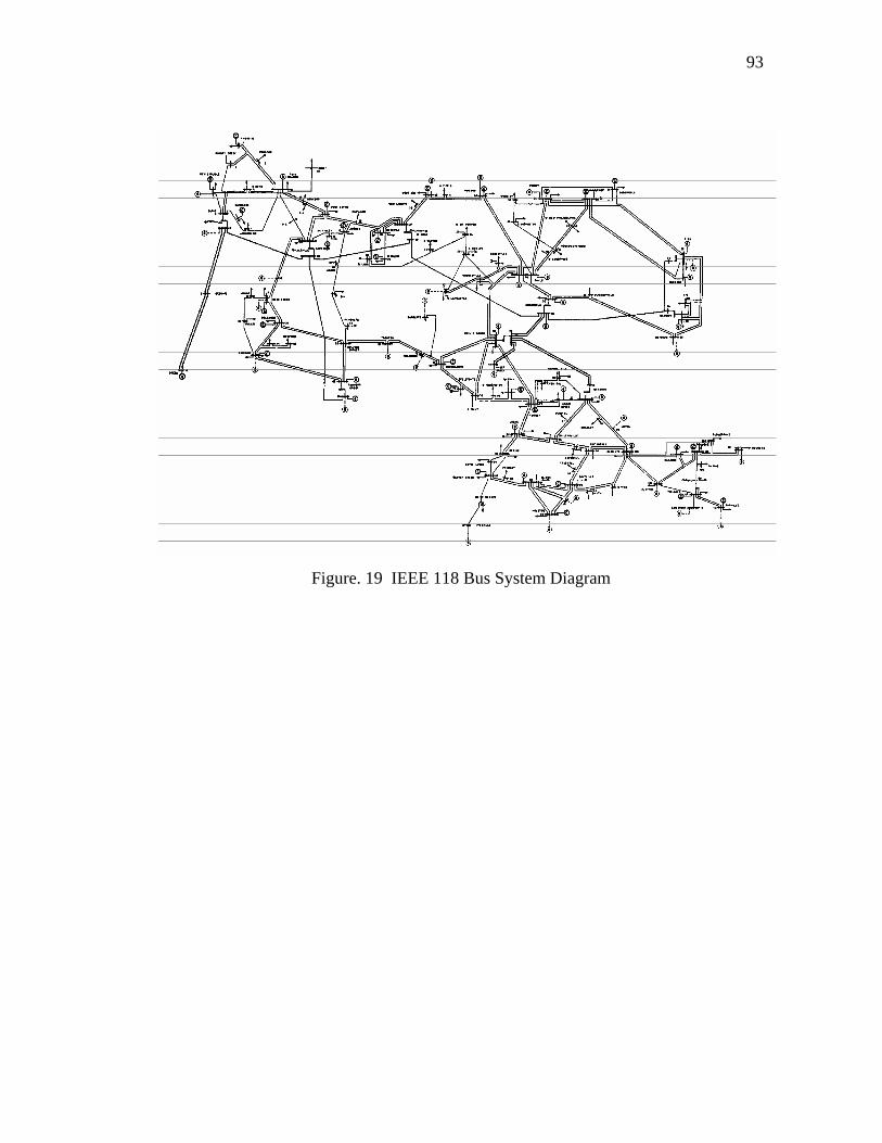
93
Figure. 19 IEEE 118 Bus System Diagram

94
VITA
Liang Zhao was born in Haimen, JiangSu province of P.R.China. He received his
Bachelor of Science degree in electrical engineering from Tsinghua Unversity in July
1994. He continued his studies as a graduate student and research assistant at Tsinghua
University during 1996-1998 and received the Master of Science degree in electrical
engineering in July 1998. Since September 2000, he has been with Texas A&M
University, working towards his Doctor of Philosophy degree in the Electrical
Engineering Department. During his Ph.D. program, he worked as Graduate Research
Assistant for the PSERC project, Graduate Assistant Non Teaching for the ELEN-460.
His research interests include power market, power system operation and planning. He is
a student member of the IEEE, the IEEE Power Engineering Society.
His permanent address is:
Liang Zhao
12, Hetang, Baochang
Haimen, JiangSu 226154
P.R.China