multi-criteria decision making under uncertain evaluations · multi-criteria decision making under...
TRANSCRIPT

Multi-Criteria Decision Making under Uncertain
Evaluations
Hesham Fahad A. Maghrabie
A thesis
in
The Concordia Institute
for
Information & Systems Engineering
Presented in Partial Fulfillment of the Requirements
For the Degree of
Doctor of Philosophy (Information and Systems Engineering) at
Concordia University
Montreal, Quebec, Canada
July 2018
© Hesham Fahad A. Maghrabie, 2018

CONCORDIA UNIVERSITY
SCHOOL OF GRADUATE STUDIES
This is to certify that the thesis prepared
By: Hesham Fahad A. Maghrabie
Entitled: Multi-Criteria Decision Making Under Uncertain Evaluations
and submitted in partial fulfillment of the requirements for the degree of
Doctor of Philosophy (Information and Systems Engineering)
complies with the regulations of the University and meets the accepted standards with respect to originality and
quality.
Signed by the final examining committee:
Chair
Dr. Ketra Schmitt
External Examiner
Dr. George Adbul-Nour
External to Program
Dr. Onur Kuzgunkaya
Examiner
Dr. Amin Hammad
Examiner
Dr. Nizar Bouguila
Thesis Co-Supervisor
Dr. Andrea Schiffauerova
Thesis Co-Supervisor
Dr. Yvan Beauregard
Approved by -
Dr. Chadi Assi, Graduate Program Director
Thursday, September 6, 2018
Dr. Amir Asif, Dean
Faculty of Engineering and Computer Science
iii
Abstract
Multi-Criteria Decision Making under Uncertain Evaluations
Hesham Fahad A. Maghrabie, Ph.D.
Concordia University, 2018
Multi-Criteria Decision Making (MCDM) is a branch of operation research that aims to
empower decision makers (DMs) in complex decision problems, where merely depending on DMs
judgment is insufficient. Conventional MCDM approaches assume that precise information is
available to analyze decision problems. However, decision problems in many applications involve
uncertain, imprecise, and subjective data.
This manuscripts-based thesis aims to address a number of challenges within the context of
MCDM under uncertain evaluations, where the available data is relatively small and information
is poor. The first manuscript is intended to handle decision problems, where interdependencies
exist among evaluation criteria, while subjective and objective uncertainty are involved. To this
end, a new hybrid MCDM methodology is introduced, in which grey systems theory is integrated
with a distinctive combination of MCDM approaches. The emergent ability of the new
methodology should improve the evaluation space in such a complex decision problem.
The overall evaluation of a MCDM problem is based on alternatives evaluations over the
different criteria and the associated weights of each criterion. However, information on criteria
weights might be unknown. In the second manuscripts, MCDM problems with completely
unknown weight information is investigated, where evaluations are uncertain. At first, to estimate
the unknown criteria weights a new optimization model is proposed, which combines the
maximizing deviation method and the principles of grey systems theory. To evaluate potential
alternatives under uncertain evaluations, the Preference Ranking Organization METHod for
Enrichment Evaluations approach is extended using degrees of possibility.

iv
In many decision areas, information is collected at different periods. Conventional MCDM
approaches are not suitable to handle such a dynamic decision problem. Accordingly, the third
manuscript aims to address dynamic MCDM (DMCDM) problems with uncertain evaluations over
different periods, while information on criteria weights and the influence of different time periods
are unknown. A new DMCDM is developed in which three phases are involved: (1) establish
priorities among evaluation criteria over different periods; (2) estimate the weight of vectors of
different time periods, where the variabilities in the influence of evaluation criteria over the
different periods are considered; (3) assess potential alternatives.

v
Acknowledgments
I would like to express my sincere appreciation to everyone who inspired me throughout my
PhD journey, especially my supervisors, Dr. Andrea Schiffauerova, from Concordia University,
and Dr. Yvan Beauregard, from École de technologie supérieure, Université du Québec. They have
taught me how to have a growth mindset and carry out a meaningful research. I am forever grateful
for their supports, valuable guidance, encouragement, and commitments.
I would also like to thank my PhD committee members, Prof. Amin Hammad, Prof. Nizar
Bouguila, and Dr. Onur Kuzgunkaya from Concordia University, for their discussions,
constructive comments, and time, which helped me to refine and improve my thesis. I also would
like to thank Prof. Georges Abdul-Nour my external examiner from Université du Québec à Trois-
Rivières, for his time and dedicated work in examining my thesis.
I would like to offer my deepest gratitude and appreciation to my wonderful parents, Mrs.
Manal Mattar and Mr. Fahad Maghrabie, for their continuous support, immense love, ultimate
kindness, and phenomenal faith in me, which have motivated me to strive toward my full potential.
However, words cannot express my incredible appreciation and gratitude to them.
I would also like to offer my endless gratitude and appreciation to my soulmate, Dr. Hanadi
Habibullah, for her endless love, support, care, and patience during my PhD journey. Hanadi has
made an incredible effort to successfully completing the Canadian board in the specialization of
radiation oncology, and sub-specialization in gynecologic cancers and breast cancers; while being
a wonderful and loving mother to our two children, Yousif and Manal. I am forever grateful for
her.
I would like to thank my lovely children, Yousif and Manal, for being a source of happiness
and motivation, which enormously helped me to overcome times of stress and frustration during
this journey.
I would like to extend my appreciation to my sisters, Heba, Shahad, and Hala Maghrabie; and
my brother Hani Maghrabie; and my brother in law Osama Faraj for their support, encouragement,
and believe in me.

vi
I would also like to offer special thanks and appreciation to my mother in law, Mrs. Aisha
Rozi, for her support, effort, and coming all the way from Saudi Arabia to Canada several times
to help us during tough times. Also, I would like to thank my father in law, Mr. Fouad Habibullah,
for his support, motivation, and bearing with us during the tough times.
I would also like to express my appreciation to my colleagues in Concordia University, for
their insightful discussions and valuable remarks, especially my friends, Saeed Sarencheh, Nawaf
Alhebaishi, Syed Eqbal, Dr. Tahseen Mustafa.
I would like to offer my sincere appreciation and gratitude to my close friend, Dr. Yasir Al-
Jefri, for his unlimited motivation, continuous inspiration, and invaluable guidance.
I acknowledge that comments and constructive criticisms from the anonymous reviewers of
different journal and conference committees, including Journal of Expert Systems with
Applications, Computers and Industrial Engineering International, Journal of Technological
Forecasting and Social Change, International Conference on Modeling, Optimization and
SIMulation, and Group Decision and Negotiation Annual Conference, have helped me in
enhancing and refining my research work.
I would like to thank the Saudi Ministry of Education, for providing generous financial support
during my studies. Also, I would like to extend my thanks to the Natural Sciences and Engineering
Research Council of Canada, for offering me the opportunity to participate in a collaboration
project between academia and industry through École de technologie supérieure, Université du
Québec, under the supervision of Dr. Yvan Beauregard.
Finally, I would like to thank the Canadian government and public, for providing my family
and I with a welcoming environment, which has made us so attached to Canada.

vii
Dedication
To the soul of my father, Mr. Fahad Maghrabie; my mother Mrs. Manal Mattar; my soulmate,
Dr. Hanadi Habibullah; and my lovely children, Yousif and Manal; for their boundless love,
endless support, unlimited motivation, and continuous inspiration.
viii
Table of Contents
List of Tables ................................................................................................................... x
List of Figures .................................................................................................................xii
List of Abbreviations ...................................................................................................... xiii
Chapter 1. Introduction ......................................................................................................... 1 1.1 Multi Criteria Decision Making .................................................................................................... 1
1.2 Uncertainty in MCDM .................................................................................................................. 2 1.3 MCDM with unknown weight information .................................................................................. 3
1.4 Dynamic multi-criteria decision problems .................................................................................... 3
1.5 Research Motivation ..................................................................................................................... 3
1.6 Research Objectives ...................................................................................................................... 4 1.7 Organization of the thesis ............................................................................................................. 5
Chapter 2. Grey-based Multi-Criteria Decision Analysis Approach: Addressing Uncertainty at
Complex Decision Problems ............................................................................................. 8 2.1 Introduction ................................................................................................................................... 9
2.2 Background ................................................................................................................................. 10 2.2.1 Multi-criteria decision analysis ........................................................................................... 10
2.2.2 Handling uncertainty in MCDA .......................................................................................... 12
2.3 Grey-based MCDA methodology (G-ANP-PROMETHEE II) .................................................. 15
2.3.1 Structure and model the decision problem .......................................................................... 17 2.3.2 Establish grey linguistic scales ........................................................................................... 17
2.3.3 Determine the weights of evaluation criteria ...................................................................... 18
2.3.4 Evaluate and rank feasible alternatives ............................................................................... 25
2.4 Case illustration of strategic decision making at the front end innovation for a small to medium-
sized enterprise within the Canadian quaternary sector .......................................................................... 30
2.4.1 Structure and model the decision problem .......................................................................... 30
2.4.2 Establish grey linguistic scales ........................................................................................... 31
2.4.3 Establish the priority level across criteria ........................................................................... 34 2.4.4 Evaluate and rank feasible alternatives ............................................................................... 36
2.5 Comparative Analysis ................................................................................................................. 41
2.6 Conclusion .................................................................................................................................. 45
Chapter 3. Multi-Criteria Decision-Making Problems with Unknown Weight Information under
Uncertain Evaluations ..................................................................................................... 47 3.1 Introduction ................................................................................................................................. 48 3.2 Background ................................................................................................................................. 49
3.3 Decision making method of interval grey MCDM with unknown weight information .............. 51
3.3.1 Problem description ............................................................................................................ 51
3.3.2 Normalize decision matrix .................................................................................................. 52 3.3.3 Establish criteria weights .................................................................................................... 53
3.3.4 Evaluate and rank feasible alternatives ............................................................................... 59
3.4 Illustrative example ..................................................................................................................... 61
3.5 Comparative analysis .................................................................................................................. 66

ix
3.6 Conclusion ........................................................................................................................................ 68
Chapter 4. A New Approach to Address Uncertain Dynamic Multi-Criteria Decision Problems
with Unknown Weight Information ................................................................................. 70 4.1 Introduction ................................................................................................................................. 71
4.2 Background ................................................................................................................................. 72
4.3 Decision making method of DGMCDM with unknown weight information ............................. 74
4.3.1 Problem description ............................................................................................................ 74 4.3.2 Normalize DGMCDM ........................................................................................................ 75
4.3.3 Establish criteria weights .................................................................................................... 76
4.3.4 Estimate the influence of dynamic evaluations ................................................................... 80
4.3.5 Evaluate and rank feasible alternatives ............................................................................... 83 4.4 Illustrative example ..................................................................................................................... 85
4.5 Comparative analysis .................................................................................................................. 89
4.6 Conclusion .................................................................................................................................. 90
Chapter 5. Conclusions, Contributions and Future Research .................................................. 92 5.1 Concluding remarks .................................................................................................................... 92
5.2 Conceptual contributions ............................................................................................................ 93
5.3 Methodological contributions ..................................................................................................... 94
5.4 Ideas for future research .............................................................................................................. 96 5.5 Related publications .................................................................................................................... 96
References ........................................................................................................................... 98

x
List of Tables
Table 2.1: Pairwise preference scale. ............................................................................................ 18
Table 2.2: Performance evaluation scale over qualitative criteria. ............................................... 19
Table 2.3: Consistency indices for a randomly generated matrix. ................................................ 22
Table 2.4: Influence matrix. .......................................................................................................... 23
Table 2.5: Evaluation criteria. ....................................................................................................... 32
Table 2.6: Interdependencies between sub-criteria. ...................................................................... 33
Table 2.7: Inner-dependencies among main criteria with respect to Market. ............................... 34
Table 2.8: Inner-dependence weights matrix of the main criteria. ............................................... 35
Table 2.9: Supermatrix.................................................................................................................. 36
Table 2.10: Weighted supermatrix. ............................................................................................... 37
Table 2.11: Evaluation of potential innovation projects on qualitative criteria. ........................... 38
Table 2.12: Evaluation of potential innovation projects on quantitative criteria. ......................... 38
Table 2.13: Normalized Performance matrix................................................................................ 39
Table 2.14: Multi-criteria preference matrix of A1. ...................................................................... 40
Table 2.15: Relative preference matrix. ........................................................................................ 40
Table 2.16: Global preference matrix - Outranking flows computations. .................................... 41
Table 2.17: Grey paired comparison matrix between dimensions. ............................................... 41

xi
Table 2.18: Criteria weights of the proposed methodology and the existing methodology. ........ 42
Table 2.19: Sub-criteria weights. .................................................................................................. 43
Table 2.20: Grey decision matrix of supplier selection. ............................................................... 44
Table 2.21: Relative preference matrix. ........................................................................................ 45
Table 2.22: Global preference matrix - Outranking flows computations. .................................... 45
Table 3.1: Uncertain decision matrix ............................................................................................ 62
Table 3.2: Normalized uncertain decision matrix ......................................................................... 63
Table 3.3: Preference matrix of A1 ............................................................................................... 63
Table 3.4: Preference matrix of A2 ............................................................................................... 64
Table 3.5: Preference matrix of A3 ............................................................................................... 64
Table 3.6: Preference matrix of A4 ............................................................................................... 65
Table 3.7: Relative preference matrix ........................................................................................... 65
Table 3.8: Outranking flows computations ................................................................................... 65
Table 3.9: Criteria weights using different approaches ................................................................ 66
Table 4.1: Uncertain decision matrix at each period .................................................................... 86
Table 4.2: Normalized uncertain decision matrix at each period ................................................. 87
Table 4.3: Preference matrix of A1 over T1 .................................................................................. 88
Table 4.4: Relative preference matrix of A1 over T1 .................................................................... 89

xii
List of Figures
Figure 1.1: Thesis framework. ........................................................................................................ 7
Figure 2.1: Analytic framework of G-ANP-PROMETHEE II. .................................................... 16
Figure 2.2: Network structure model. ........................................................................................... 17
Figure 2.3: Network structure of the evaluation criteria within the context of FEI...................... 33

xiii
List of Abbreviations
𝜆𝑚𝑎𝑥 Largest eigenvalue
AHP Analytic Hierarchy Process
ANP Analytical Network Process
BUM Basic Unit-interval Monotonic
CI Consistency Index
CR Consistency Ratio
DFMCDM Dynamic Fuzzy Multiple Criteria Decision Making
DGMCDM Dynamic Grey Multi-Criteria Decision Making
DIFWA∊ Dynamic Intuitionistic Fuzzy Einstein Averaging
DIFWG∊ Dynamic Intuitionistic Fuzzy Einstein Geometric Averaging
DIFWG Dynamic Intuitionistic Fuzzy Weighted Geometric
DMCDM Dynamic Multi-Criteria Decision Making
DMs Decision Makers
ELECTRE ELimination and Choice Expressing REality

xiv
FAHP Fuzzy Analytic Hierarchy Process
FEI Front End Innovation
GANP Grey Analytical Network process
GRA Grey Relational Analysis
GWSM Grey Weighted Sum Model
LINMAP Linear Programming Technique for Multidimensional Analysis of
Preference
MADA Multi-Attribute Decision Analysis
MAUT Multi-Attribute Utility Theory
MAVT Multi-Attribute Value Theory
MCA Multi-Criteria Analysis
MCDA Multi-Criteria Decision Analysis
MCDM Multi-Criteria Decision Making
PROMETHEE II Preference Ranking Organization METHod for Enrichment Evaluation II
𝑅𝐼 Consistency Index of a Random-like Matrix
SMAA Stochastic Multi-criteria Acceptability Analysis
xv
SMART Simple Multi-Attribute Rating Technique
TOPSIS Technique for Order Preference by Similarity to Ideal Solution
UDIFWG Uncertain Dynamic Intuitionistic Fuzzy Weighted Geometric
VIKOR Vlsekriterijumska Optimizacijia I Kompromisno Resenje
WSM Weighted Sum Method

1
Chapter 1
Introduction
1.1 Multi Criteria Decision Making
Decision making is an inherent character of human nature. The ultimate goal of any decision
maker is to make the right decision. Sometimes the process of undertaking the right decision
becomes a challenging task, especially when they encounter large amount of complex information.
Therefore, tremendous efforts have been dedicated to enrich the decision making process by
introducing multi-criteria analysis (MCA) approaches. The main role of MCA is to handle the
associated difficulties with decision problems where the ability of decision makers (DMs) are
deemed insufficient by itself to address the decision problems (Dodgson, Spackman, Pearman, &
Phillips, 2009). MCA can be defined as structured approaches for DMs to have a thorough analysis
over decision problems by analyzing and evaluating potential alternatives over a set of criteria
(Antunes & Henriques, 2016; Kurka & Blackwood, 2013).
Many approaches of MCA are available in the literature. However, different reasons justify the
existing of the different approaches (Dodgson et al., 2009):
• the dissimilarity among decisions in nature and purpose
• the available time for making a decision
• the nature of the data and its availability
• the analytical skills of the DMs
• the various type of administrative culture.
Among the popular approaches of MCA is the multi-criteria decision making (MCDM), also
known as multi-criteria decision analysis (MCDA) and multi-attribute decision analysis (MADA)
(Dodgson et al., 2009). The main role of MCDM is to aid DMs in establishing a coherent picture
about complex decision problems, e.g. decision problems that incorporate monetary and non-
monetary criteria (Kurka & Blackwood, 2013; Malczewski & Rinner, 2015; Roy, 2016; Wątróbski
& Jankowski, 2016). Moreover, it simplifies the analysis of a decision problem by disaggregating

2
the original problem into more manageable elements (Dodgson et al., 2009; Kurka & Blackwood,
2013).
A defined decision making problem can be categorized based on the problematic nature as
follows (Greco, Ehrgott, & Figueira, 2016; Wątróbski & Jankowski, 2016):
1. Choice problematic: Finding the best alternative
2. Sorting problematic: Sorting alternatives into defined categories
3. Ranking problematic: Ranking alternatives from the best to the worst.
Despite the diversity of MCDM approaches, at the most primitive level, MCDM can be
demonstrated by a set of alternatives, at least two evaluation criteria, and minimally one decision
maker (Greco et al., 2016).
1.2 Uncertainty in MCDM
Conventional MCDM approaches presume that the required information for analyzing a
decision problem is available and accurate. However, in many real life applications available
information is subject to uncertainty, imprecision, and subjectivity; which would limit the
applicability of conventional MCDM approaches (Banaeian, Mobli, Fahimnia, & Nielsen, 2018;
Karsak & Dursun, 2015; Guangxu Li, Kou, & Peng, 2015; Małachowski, 2016). Consequently,
different theories have been introduced to approximate ranges of evaluations using the related
knowledge and the available information of the decision problem under consideration (Lin, Lee,
& Ting, 2008).
The different approaches to address uncertainty have different use, which involves the way of
establishing preferences within a decision problem and the way of representing possible outcomes
(Durbach & Stewart, 2012). Therefore, differentiating among two types of uncertainty would be
useful to properly handle the associated uncertainty in a decision problem. The two types of
uncertainty are: (i) uncertainty associated with limited objective information, e.g., quantitative
(interval scales) and stochastic (probability distribution) data, and (ii) uncertainty associated with
subjective expert knowledge (i.e., ambiguous concepts and semantic meanings) (Malczewski &
Rinner, 2015; Moretti, Öztürk, & Tsoukiàs, 2016).
3
1.3 MCDM with unknown weight information
Solving a MCDM requires information on alternatives evaluations over the different criteria
and the associated weight of each criterion. Within the context of uncertain MCDM problems,
decision makers may encounter decision problems with unknown criteria weights, as a result of
different reasons such as time pressure, limited expertise, incomplete knowledge, and lack of
information (Das, Dutta, & Guha, 2016; S. Zhang, Liu, & Zhai, 2011). Accordingly, the overall
evaluations cannot be derived (Xu, 2015).
1.4 Dynamic multi-criteria decision problems
Conventional MCDM approaches have an implicit assumption in which decision problems are
static overtime (single period) (Pruyt, 2007). However, in many real-life applications this
assumption becomes inappropriate as decision information is provided at different periods such as
multi-period investment and medical diagnosis (Eren & Kaynak, 2017; G. Wei, 2011). In such
decision areas, the complexity of decision making process increases and requires the consideration
of different evaluations over the different periods.
1.5 Research Motivation
The associated uncertainty with many real-life applications of MCDM problems complicates
the decision-making process, in which it renders conventional MCDM approaches to be incapable
of addressing the multi-criteria decision problems (Banaeian et al., 2018; Karsak & Dursun, 2015;
Guangxu Li et al., 2015; Małachowski, 2016). Consequently, different hybrid methodologies have
been introduced, in which MCDM approaches have been supplemented by different methods to
handle the different types of uncertainty; such as probabilistic models, fuzzy set theory, and grey
systems theory. However, the existing methodologies are limited when it comes to handle MCDM
problems with a relatively small amount of data and poor information, where evaluation criteria
are of different nature and interdependencies exist among them.
As mentioned earlier, information on criteria weights is critical to solve MCDM problems (Xu,
2015). However, in many decision problems criteria weights are unknown (Das et al., 2016; S.
Zhang et al., 2011). Therefore, different approaches have been introduced to establish the unknown

4
criteria weights, which are listed in Chapter 3. Nevertheless, the applicability of these approaches
would be influenced when it comes to handle MCDM problems with small amount of data and
poor information.
In many decision areas information at different periods should be considered, such as multi-
period investment and medical diagnosis (G. Wei, 2011). Conventional MCDM approaches are
static and cannot handle dynamic decision problems. Different hybrid approaches have been
developed to overcome the shortcoming of the conventional approaches, which are mentioned in
Chapter 4. However, the developed approaches lack of a proper procedure to address one or both
of the following concerns: (1) Criteria weights establishment, where weight information is
unknown; (2) Establishing priorities of different periods, where the influence on a decision
problem of different evaluation criteria are changing over time.
In view of the aforementioned limitations, it is important to establish a decision model that
consider the interdependencies among evaluation criteria within the context of MCDM problems
with a relatively small amount of data and poor information. For decision problems with unknown
criteria weights a better method is needed to establish unknown criteria weights, where information
is poor and the available data is relatively small. In a multi-period MCDM where priority
information of different periods is unknown, the changing in the influence of the different
evaluation criteria over different periods should be considered in solving the dynamic decision
problems.
1.6 Research Objectives
This manuscript-based thesis consists of three journal papers, each of which will be discussed
in a separate chapter. The objectives of each paper are as follows:
➢ Paper 1: Grey-based Multi-Criteria Decision Analysis Approach: Addressing Uncertainty at
Complex Decision Problems
The ultimate goal of this research is to optimize the evaluation space in complex MCDM that
are subject to subjective and objective uncertainty over different types of interrelated criteria. To
this end, the main objective of this paper are as follows: prioritize interrelated criteria of different

5
nature, while uncertainty related aspects are present; evaluate different alternatives over complex
MCDM problems under subjective and objective uncertainty.
➢ Paper 2: Multi-Criteria Decision-Making Problems with Unknown Weight Information under
Uncertain Evaluations
The aim of this paper is to handle MCDM problems with small amount of data and poor
information, where information of criteria weights is unknown. Therefore, the objectives of this
paper are as follows: establish a new optimization model to estimate priorities among the
evaluation criteria under such a decision problem; evaluate and rank potential alternatives, where
uncertain information with respect to alternatives evaluations is provided.
➢ Paper 3: A New Approach to Address Uncertain Dynamic Multi-Criteria Decision Problems
with Unknown Weight Information
This paper aims to address a dynamic MCDM, where evaluations are given over different
periods, while information on criteria weights and the influence of different time periods are
unknown. Consequently, the objectives of this paper are as follows: prioritize criteria weights over
the different periods; establish weight vectors of different periods while considering the
variabilities in the influence of different criteria over different periods.
1.7 Organization of the thesis
This manuscript-based thesis is divided into five chapters. Chapter 1 provides a brief
background on related subject matters to introduce the motivations and objectives of this thesis.
The objectives of this thesis have been carried-out through Chapters 2 to 4, as outlined below:
Chapter 2: Grey-based Multi-Criteria Decision Analysis Approach: Addressing Uncertainty at
Complex Decision Problem. In this chapter, a new hybrid MCDM model is developed to better
address complex decision problems with relatively small amount of data and poor information.
The proposed methodology considers the interdependencies among the evaluation criteria of
different clusters while establishing criteria weights. Moreover, it extends the approach of
Preference Ranking Organization METHod for Enrichment Evaluation II (PROMETHEE II), in

6
which it would be utilized to define optimal ranking among potential alternatives in complex
decision problem under subjective and objective uncertainty.
Chapter 3: Multi-Criteria Decision-Making Problems with Unknown Weight Information
under Uncertain Evaluations. This chapter introduces a new methodology to carry out the overall
evaluation for MCDM problems with small amount of data and poor information, where
information on criteria weight is unknown completely. A new optimization model is developed to
establish criteria weights, while different scenarios are considered to generalize the model.
Chapter 4: A New Approach to Address Uncertain Dynamic Multi-Criteria Decision Problems
with Unknown Weight Information. A new methodology is proposed in this chapter to account for
the dynamic aspect of a MCDM, where evaluations from different periods are provided, while
information on criteria weights and the influence of the different periods are unknown completely.
The new approach pays attention to the variabilities in the influence of different evaluation criteria
on a MCDM problem over different periods.
Finally, Chapter 5 provides a summary of this thesis including the concluding remarks,
contributions and ideas for future research. The analytical framework of the thesis is illustrated in
Figure 1.1.

7
Figure 1.1: Thesis framework.
Static No Yes
Information on
interrelated
criteria
Multi-Criteria Decision
Making under Uncertain
Evaluations
No Yes
Chapter 3
MCDM with Unknown
Weight Information under
Uncertain Evaluations
Chapter 2
Grey-based Multi-Criteria
Decision Analysis Approach
Chapter 4
A New Approach to Address
Uncertain DMCDM with
Unknown Weight Information
• Establish deviation matrix
over multiple periods
• Estimate optimal criteria
weights over multiple
periods
• Construct optimization
DMCDM model
• Estimate the influence of the
dynamic evaluations
• Evaluate and rank visible
alternatives
• Establish deviation matrix
• Construct optimization
MCDM model
• Determine optimal criteria
weights
• Evaluate and rank visible
alternatives
• Structure & model decision
problem
• Establish grey linguistic scale
• Determine criteria weights
• Evaluate and rank visible
alternatives

8
Chapter 2
Grey-based Multi-Criteria Decision Analysis Approach:
Addressing Uncertainty at Complex Decision Problems
Abstract
In complex systems, decision makers encounter uncertainty from various sources. Grey
systems theory is recommended to address uncertainty for decision problems with a relatively
small amount of data (i.e., small samples) and poor information, which cannot be described by a
probability distribution. However, the existing approaches do not consider the influence among
criteria of different clusters. Accordingly, a new hybrid grey-based Multi-Criteria Decision
Analysis (MCDA) approach is proposed to optimize the evaluation space in decision problems
that are subject to subjective and objective uncertainty over different types of interrelated criteria.
The four-phased methodology begins with the formulation of a decision problem through the
analysis of the system of concern, its functionality, and substantial connections among criteria.
The second phase involves the development of grey linguistic scales to handle uncertainty of
human judgments. The third phase integrates the grey linguistic scale, concepts of grey systems
theory, and principles of Analytical Network Process to prioritize the evaluation criteria. Finally,
to evaluate and rank alternatives in such a complex setting, the Preference Ranking Organization
METHod for Enrichment Evaluation II approach is extended using a grey linguistic scale to
articulate subjective measures over qualitative criteria, grey numbers to account for objective
uncertainty over quantitative criteria, grey operating rules to normalize evaluation measures, and
the proposed approach of prioritizing the criteria to establish relative preferences. To demonstrate
the viability of the methodology, a case study is presented, in which a strategic decision is made
within the context of innovation. To validate the methodology, a comparative analysis is provided.

9
2.1 Introduction
Decision makers usually encounter large amount of complex information. The complexity of
decision problems increases when different evaluation criteria of different nature (e.g., qualitative
and quantitative), different scales, and different values (e.g., continuous, discrete, and linguistic)
are involved.
Multi-Criteria Decision Analysis (MCDA) is therefore considered one of the most fruitful sub-
disciplines of operations research. The main role of MCDA is to aid Decision Makers (DMs) in
establishing a coherent picture about complex decision problems (Kurka & Blackwood, 2013).
However, in many cases uncertainty-related aspects (i.e., uncertainty associated with limited
objective information and uncertainty associated with subjective expert knowledge) are present.
This adds to the complexity of analyzing the decision problems as the conventional MCDA
approaches presume the availability of precise information (Kuang, Kilgour, & Hipel, 2015; Guo-
dong Li, Yamaguchi, & Nagai, 2007).
Various methods have been proposed to deal with different types of uncertainty-related
aspects. Grey systems theory is recommended for decision problems with a relatively small
amount of data (i.e., small samples) and poor information, which cannot be described by a
probability distribution (C. Li & Yuan, 2017; D.-C. Li, Chang, Chen, & Chen, 2012; S. Liu & Lin,
2006). Accordingly, different researchers have considered the grey systems theory to address
uncertainty in decision problems, as presented in the next section. The existing approaches
assumed that DMs are able to assign the weights of the evaluation criteria precisely, did not
consider the interrelationships among evaluation criteria, or did not consider the relations among
the criteria of different clusters, hence a better method is needed to address the existing research
gaps.
The ultimate goal of this research is to enhance DMs abilities of handling multi-criteria
decision problems under uncertainty. To this end, the main objective of this manuscript is to
establish a structured methodology, which are able to carry on MCDA under uncertainty, by
integrating the grey systems theory with a distinctive combination of MCDA techniques (i.e.,
Analytical Network Process (ANP) and Preference Ranking Organization METHod for

10
Enrichment Evaluation II (PROMETHEE II)). The hybrid methodology uses the grey systems
theory as the key element for tackling uncertainty aspects; the principles of ANP to handle the
complexity of the decision structure; the extended PROMETHEE II approach to evaluate feasible
alternatives.
The contributions of this manuscript over other existing research works within the same
context of MCDM problems can be summarized in the following points: (1) Establishing priorities
among sub-criteria within a complex structure under uncertain subjective judgments using the
combination of linguistic expression, grey systems theory, and the principles of ANP; (2)
Extending PROMETHEE II, such that potential alternatives can be evaluated and ranked in such
a complicated decision structure; (3) Improving the evaluation space in a complex decision
problems under uncertainty by utilizing the emergent strengths of the integrated approach, which
would enhance the evaluation of a DM.
This manuscript is organized as follows: first, a brief background on related subject matters is
provided to identify the research problems and to establish the direction of the current research;
next, the proposed methodology is discussed and explained; afterwards, a case study is presented
to demonstrate the viability of the methodology; then, a comparative analysis with an existing
approach is performed for the validation purpose; finally, the conclusion is put forward.
2.2 Background
2.2.1 Multi-criteria decision analysis
Despite the diversity of MCDA approaches, at the most primitive level, MCDA can be
demonstrated by a set of alternatives, at least two evaluation criteria, and minimally one decision
maker (Greco et al., 2016). Accordingly, MCDA can be described as a systematic methodology
that helps in making decisions by evaluating a number of alternatives over a set of criteria
according to the preferences of the involved decision maker(s).
There is no optimal MCDA’s approach that would fit perfectly with every decision problem.
Therefore, understanding a decision problem’s nature is a critical step to identify the suitable

11
approach for it (Jaini & Utyuzhnikov, 2017; Wątróbski & Jankowski, 2016). The various
approaches of MCDA can be classified into three main categories (Belton & Stewart, 2002):
• Value measurement models: Approaches that belong to this category are value-focused,
where the utility value of each alternative is being recognized based on its overall performance
over the evaluation criteria. Among the most common approaches within this category are
Analytic Hierarchy Process (AHP), Analytic Network Process (ANP), Multi-Attribute Value
Theory (MAVT), Multi-Attribute Utility Theory (MAUT), Simple Multi-Attribute Rating
Technique (SMART), Stochastic Multi-criteria Acceptability Analysis (SMAA), and
Weighted Sum Method (WSM).
• Goal, aspiration, or reference-level models: In this set of approaches, alternatives are
evaluated with respect to a targeted level of performance over a particular goal, aspiration, or
reference levels, e.g., goal programming and heuristic algorithms. An example of this category
is Technique for Order Preference by Similarity to Ideal Solution (TOPSIS), Vlsekriterijumska
Optimizacijia I Kompromisno Resenje (VIKOR), and Linear Programming Technique for
Multidimensional Analysis of Preference (LINMAP).
• Outranking methods: A typical outranking approach performs pairwise comparisons between
alternatives across a specified set of evaluation criteria. Subsequently, the resulting
comparisons are aggregated and analyzed in accordance with the designated approach to favor
one alternative over another. Outranking methods include ELimination and Choice Expressing
REality (ELECTRE), and Preference Ranking Organization METHod for Enrichment
Evaluations (PROMETHEE) family of methods.
These conventional approaches of MCDA have an implicit assumption, which presumes the
availability and accuracy of information that is required for analyzing decision problems.
However, in real world applications, DMs encounter uncertainty from various sources, such as
limited human cognition, lack of understanding for interrelationships among decision criteria, and
limited input data (Belton & Stewart, 2002; Małachowski, 2016).

12
2.2.2 Handling uncertainty in MCDA
While the presence of uncertainty would limit the utilization of the MCDA approaches, several
research works have proposed different hybrid approaches, in which MCDA techniques have been
supplemented by uncertainty approaches. However, different uncertainty approaches have
different use, which involves the way of establishing preferences within a decision problem and
the way of representing possible outcomes (Durbach & Stewart, 2012). Therefore, differentiating
among two types of uncertainty would be useful to properly address the associated uncertainty in
a decision problem: (i) uncertainty associated with limited objective information, e.g., quantitative
(interval scales) and stochastic (probability distribution) data, and (ii) uncertainty associated with
subjective expert knowledge (i.e., ambiguous concepts and semantic meanings) (Malczewski &
Rinner, 2015; Moretti et al., 2016). Different approaches have been proposed to handle different
types of uncertainty:
Probabilistic models: A DM can assign probability distribution based on a relative experiences,
beliefs, and available data to describe uncertain values (i.e., imperfect information) of a decision
parameters (Mazarr, 2016). Consequently, comparisons can be established among feasible
alternatives and probabilistic statements can be made to describe the probability of occurrence for
each outcome, which can be achieved through different means (e.g., Monte Carlo simulation)
(Malczewski & Rinner, 2015; Zhou, Wang, & Zhang, 2017).
Fuzzy set theory: Zadeh (1965) introduced this theory to handle the associated vagueness and
imprecision with human judgments (i.e., ambiguous concepts and semantic meanings). Within the
context of MCDA, fuzzy numbers are utilized to map linguistic expressions that would express
human opinions using the concept of the membership function, such that by assigning a value
between 0 and 1 the linguistic term can be stated more precisely, where 0 indicates no membership
and 1 indicates full membership (Dincer, Hacioglu, Tatoglu, & Delen, 2016).
Grey systems theory: Ju-long (1982) introduced the grey systems theory as a methodology to
handle data imprecision or insufficiency in a system. It is intended for problems that involve a
relatively small amount of data and poor information, which cannot be described by a probability
distribution. Thus, a better understanding for such a system can be achieved through partially

13
known information using grey systems theory (S. Liu, Forrest, & Yang, 2015). Similar to fuzzy
set theory, grey systems theory can handle associated vagueness with verbal statements (linguistic
expressions) using grey numbers (Broekhuizen, Groothuis-Oudshoorn, Til, Hummel, & IJzerman,
2015), which is denoted by ⊗ (S. Liu & Lin, 2006).
As mentioned earlier, conventional MCDA approaches do not mimic the functional reality of
the human cognitive system in decision problems. Therefore, various hybrid approaches have been
proposed, in which uncertainty related aspects in MCDA are captured and represented using
probabilistic models, fuzzy set theory, and grey systems theory.
Fuzzy set theory is widely utilized with MCDA under uncertainty (Broekhuizen et al., 2015).
For instance, fuzzy AHP was used extensively in the literature: environmental impact assessment
(Ruiz-Padillo, Ruiz, Torija, & Ramos-Ridao, 2016), investment decisions (Dincer et al., 2016),
knowledge management (K.Patil & Kant, 2014); fuzzy ANP has been utilized to determine the
most important factors for a hospital information system (Mehrbakhsh, Ahmadi, Ahani,
Ravangard, & Ibrahim, 2016); fuzzy TOPSIS has been employed for the selection of renewable
energy supply system (Şengül, Eren, Shiraz, Gezderd, & Şengül, 2015); fuzzy VIKOR has been
used for evaluating and selecting green supplier development programs (Awasthi & Kannan,
2016); fuzzy PROMETHEE has been utilized to select the best waste treatment solution (Lolli et
al., 2016). However, the Probabilistic approach is commonly used with SMAA to provide the
specification of distributions (Groothuis-Oudshoorn, Broekhuizen, & van Til, 2017).
Although probabilistic models and fuzzy set theory are intended to investigate uncertain
systems, grey systems theory is preferred when it comes to problems with a relatively small amount
of data and poor information, which cannot be described by a probability distribution (C. Li &
Yuan, 2017; D.-C. Li et al., 2012; S. Liu & Lin, 2006), due to its less restricted procedure that
neither requires any robust membership function, nor a probability distribution (Memon, Lee, &
Mari, 2015). Consequently, several research papers have proposed grey systems theory to
supplement the deficiencies that exist in MCDA as a result of poor information. The rest of this
section deliberates on existing methods to solve multi-criteria decision problems under uncertainty
using grey systems theory, and the reasoning behind the proposed methodology.

14
Grey systems theory has been integrated with PROMETHEE II to evaluate performance of
available alternatives on certain criteria where uncertainty aspects are involved (Kuang et al.,
2015). However, the weights of evaluation criteria are assumed to be given by DMs precisely,
which is hardly the case in complex decision problems under uncertainty. Some other works have
tried to address this issue by integrating the grey systems theory with Analytic Hierarchy Process
(AHP) to prioritize evaluation criteria and to evaluate potential alternatives under uncertainty
(Jianbo, Suihuai, & Wen, 2016; Thakur & Ramesh, 2017). Also, Grey Relational Analysis (GRA),
which is a branch of grey systems theory, has been combined with the Technique for Order
Preference by Similarity to Ideal Solution (TOPSIS) approach to better rank feasible alternatives,
using fuzzy analytic hierarchy process (FAHP) to evaluate the criteria weights (Celik, Erdogan,
& Gumus, 2016; Sakthivel et al., 2014). Nevertheless, one of the underlying assumptions of AHP
is the independency (Ishizaka & Labib, 2011), which implies that elements of a hierarchal structure
are independent but in reality a complex system usually involves interactions and dependencies
among the system’s elements.
To tackle the problem of dependencies in a complex system, grey systems theory has been
used with ANP. This combination has been proposed in different areas such as, green supplier
development programs (Dou, Zhu, & Sarkis, 2014), R&D system development for a home
appliances company (Tuzkaya & Yolver, 2015), and early evaluation model for storm tide risk
(W. Zhang, Zhang, Fu, & Liu, 2009). However, the relations between sub-criteria of different
clusters have not been considered. Accordingly, a better method is needed to bridge the existing
research gaps.
In this manuscript, a new hybrid grey-based MCDA approach is proposed to enhance DMs
abilities of handling multi-criteria decision problems under uncertainty. The proposed approach
integrates the grey systems theory with a distinctive combination of MCDA (i.e., ANP and
PROMETHEE II). The combination of the proposed methodology has been considered for the
following reasons:
When it comes to performance evaluation of feasible alternatives, outranking approaches
outperform other MCDA methodologies, as other methodologies are designed to enrich the
dominance graph by reducing the number of incomparability and allocating an absolute utility to

15
each alternative. Consequently, the original structure of a multi-criteria decision problem would
be reduced to a single criterion problem for which an optimal solution exists (Maity &
Chakraborty, 2015). In contrast, outranking methods preserve the structure of multi-criteria
decision problems by considering the deviation between the evaluations of feasible alternatives
over each criterion (Andreopoulou, Koliouska, Galariotis, & Zopounidis, 2017; Maity &
Chakraborty, 2015; Segura & Maroto, 2017). Moreover, this category of MCDA can handle
quantitative and qualitative criteria. Furthermore, it requires a relatively small amount of
information from DMs (Malczewski & Rinner, 2015). Among the outranking methods,
PROMETHEE is preferred due to its mathematical properties and simplicity (Brans & De Smet,
2016; Kilic, Zaim, & Delen, 2015; Malczewski & Rinner, 2015). Among the PROMETHEE
family of methods, PROMETHEE II is preferred due to its ability of providing a complete ranking
for available alternatives based on outranking relations (Sen, Datta, Patel, & Mahapatra, 2015).
However, PROMETHEE II requires the weights of the evaluation criteria (Brans & De Smet,
2016; Segura & Maroto, 2017).
To estimate criteria weights, ANP is preferred over other MCDA approaches due to its
superiority in addressing different types of interrelationships (e.g., interactions and
interdependencies) within and between different evaluation clusters of a complex system (Hsu,
2015; Tuzkaya & Yolver, 2015).
While the presence of uncertainty would limit the utilization of the conventional approaches
of MCDA, grey systems theory would perfectly bridge this limitation (Dou et al., 2014; Kuang et
al., 2015). In particular, when it comes to address decision problems with a relatively small amount
of data and poor information, which cannot be described by a probability distribution (D.-C. Li et
al., 2012; S. Liu & Lin, 2006).
2.3 Grey-based MCDA methodology (G-ANP-PROMETHEE II)
The proposed decision analysis process (G-ANP-PROMETHEE II) is consisted of four phases: (1)
structure and model the decision problem, (2) establish grey linguistic scales, (3) determine the
weights of evaluation criteria, and (4) evaluate and rank feasible alternatives. The framework of
the proposed methodology is illustrated in Figure 2.1. The procedural steps of G-ANP-

16
PROMETHEE II are explained in the following subsections.
DM(S)CriteriaAlternatives
Phase 3: Determine criteria weights
Step 3.2
Interdependencies
(Sub criteria)
Step 3.1
Inner-dependencies
(Main criteria)
Step 3.3
Global weights
Phase 1
Structure & model
decision problem
Phase 2
Establish Grey-
linguistic scale
Phase 4: Evaluate & rank alternatives
Step 4.1
Performance Matrix
Step 4.2
Normalized Grey
Performance Matrix
Step 4.4
Relative Preference
Matrix
Step 4.3
Preference Matrix
Alternatives Ranking
Negative Outranking
Flows
Positive Outranking
Flows
Net Outranking
Flows
Figure 2.1: Analytic framework of G-ANP-PROMETHEE II.

17
2.3.1 Structure and model the decision problem
The first phase of the methodology is formulating the problem, which requires analysis for the
system of concern, its functionality, and substantial connections (i.e., connections within and
between various elements of the system; or between the system, relevant factors, and its
environment). Accordingly, the network structure can be used to model the decision problem, as
represented by Figure 2.2.
GOAL
Cluster 1
X1, X2, …, Xm
Cluster 2
X1, X2, …, Xm
Cluster 3
X1, X2, …, Xm
Alternatives
Inner-dependence
Outer-dependence
Feedback
Figure 2.2: Network structure model (Görener, 2012).
2.3.2 Establish grey linguistic scales
Multi-criteria decision problems involve some uncertainty because they are unlikely to fully
satisfy decision criteria. Also, it is difficult for DMs to precisely express preferences due to
information limitations and the uncertainty of human judgment. Therefore, linguistic expressions
are more often used in MCDA to articulate DMs’ preferences between evaluation criteria, and to
evaluate available alternatives over qualitative criteria (Kuang et al., 2015; Merigó, Palacios-
Marqués, & Zeng, 2016).

18
In this research, the concepts of grey systems theory and linguistic expressions provide the
basis for the proposed approach, in which linguistic expressions (e.g., low, medium, and high) are
used to express DMs judgments and the grey systems theory is used to handle the associated
vagueness with verbal statements through the operating rules of grey numbers.
To express preferences of DMs between evaluation criteria with respect to the system of
concern, a grey linguistic scale of six levels is proposed, as illustrated in Table 2.1. The proposed
scale has been established in accordance with the research of Ertay, Büyüközkan, Kahraman, and
Ruan (2005).
Table 2.1: Pairwise preference scale.
Pairwise linguistic scale Grey preference scale Reciprocal grey preference scale
Just equal [1,1] [1,1]
Equally important [1/2,3/2] [2/3,2]
Weakly more important [1,2] [1/2,1]
Moderately more important [3/2,5/2] [2/5,2/3]
Strongly more important [2,3] [1/3,1/2]
Extremely more important [5/2,7/2] [2/7,2/5]
When it comes to the assessment of feasible alternatives over qualitative criteria, it is also
expressed in linguistic values using a five-level scale as shown in Table 2.2.
2.3.3 Determine the weights of evaluation criteria
For a complex multi-criteria decision problem (i.e., decision problems that involves
interrelationships between evaluation criteria), ANP provides a structured procedure to analyze
such complexity in decision problems (Zaim et al., 2014). However, ANP cannot effectively
address uncertainty-related issues (Nguyen, Dawal, Nukman, & Aoyama, 2014), which are usually
present in real world applications. To overcome this limitation, linguistic expressions and concepts
19
Table 2.2: Performance evaluation scale over qualitative criteria.
Performance evaluation linguistic scale Grey evaluation scale
Low (L) [0,0.2]
Less than moderate (LM) [0.2,0.4]
Moderate (M) [0.4,0.6]
More than moderate (MM) [0.6,0.8]
High (H) [0.8,1.0]
of grey systems theory are integrated with ANP to establish the set of weights for evaluation
criteria. The procedural steps are as follows: (1) determine inner-dependencies among main
criteria, (2) examine interdependencies among sub-criteria, and (3) Estimate global weights for
sub-criteria using the outputs of steps a and b.
2.3.3.1 Determine inner-dependencies among main criteria
The purpose of inner-dependencies evaluation is to detect the relative importance among
various elements of the same level or cluster. This could be achieved by analyzing the influence
of an evaluation criterion over other elements of the same level/cluster using linguistic expressions
and relative grey numbers, as in Table 2.3, to articulate DMs’ preferences between evaluation
criteria.
2.3.3.1.1 Establish grey-based pairwise comparison matrices for main criteria
Definition 2.1 Let a set of criteria within a cluster be represented by 𝐶 = {𝐶1, 𝐶2 , … , 𝐶𝑚}, where
m is the number of criteria. Let 𝑎𝑖𝑗 indicate the existence of an influence relation of criterion 𝐶𝑖
over 𝐶𝑗, where
𝑎𝑖𝑗 = {1 ↔ 𝐶𝑖 influences 𝐶𝑗 ∨ (i = j)
0 ↔ 𝐶𝑖 𝒅𝒐𝒆𝒔 𝒏𝒐𝒕 influence 𝐶𝑗
, 𝑖, 𝑗 = 1, 2, …𝑚 (2.1)
20
Definition 2.2 Let 𝐼𝑘 represent a set of evaluation criteria that influence a criterion 𝐶𝑘, where 𝐼𝑘 ⊂
𝐶 and 𝐶𝑘 ∉ 𝐼𝑘. Let 𝑅[⊗] represent the set of grey numbers and 𝑇𝑘⊗ denote a grey description
function that describes the grey-based pairwise comparisons between elements of 𝐼𝑘 with respect
to 𝐶𝑘, such that
𝑇𝑘⊗ ∶ (𝐼𝑘 × 𝐼𝑘) → 𝑅[⊗], ∀𝑘 = 1, 2, …𝑚 (2.2)
Definition 2.3 Let 𝑘𝑖𝑗(⨂) ∈ 𝑇𝑘⊗ denote a grey number that articulates DMs’ verbal preference
of 𝐶𝑖 over 𝐶𝑗 with respect to a control criterion 𝐶𝑘, where both 𝐶𝑖 and 𝐶𝑗 influence 𝐶𝑘 and 𝑘 ≠ 𝑖, 𝑗.
Thus,
∃ 𝑘𝑖𝑗(⨂) ↔ (𝑎𝑖𝑘, 𝑎𝑗𝑘 = 1), ∀ 𝑇𝑘⊗ (𝐶𝑖, 𝐶𝑗), 𝑤ℎ𝑒𝑟𝑒 (2.3)
𝑘𝑖𝑗(⨂) = {𝑘𝑗𝑖(⨂)
−1 ↔ 𝑖 ≠ 𝑗
[1,1], otherwise , 𝑖, 𝑗, 𝑘 = 1, 2… ,𝑚
2.3.3.1.2 Estimate inner-dependence weights
To estimate the inner-dependence weights among evaluation criteria, the grey numbers at the
grey-based pairwise comparisons matrices need to be transformed to white numbers (i.e., single
values). To do this, the whitenization process should be performed.
The weight function of the whitenization process is decided based on the available information
of the relative grey numbers (e.g., distribution information), knowledge, and experience of
decision makers (S. Liu & Lin, 2006).
Definition 2.4 Assume that a whitenization function for a relative grey number 𝑥(⨂) is 𝑓(𝑥𝑖), then
the whitenization value 𝑥𝑖(⨂̃) can be defined as (Shi, Liu, & Sun, 2013):
𝑥(⨂̃) = 𝑥 . 𝑓(𝑥) (2.4)
In many practical applications, the weight function of the whitenization process is unknown
(S. Liu & Lin, 2006), which adds complexity to decision problems. Therefore, Liu and Lin (2006)
proposed the equal weight mean whitenization function to establish the associated white values of

21
interval grey numbers. In this research, the interval grey numbers are used and it is assumed that
the weight function of the whitenization process is unknown due to the lack of information.
Therefore, the equal weight mean whitenization function is considered for the whitenization
process as follows:
Definition 2.5 Let 𝑥(⨂) ∈ [𝑎, 𝑏] be a general interval grey number, where 𝑎 < 𝑏 and the
distribution information for the grey number is unknown. Let 𝛼 denote the weight coefficient. The
whitenization value 𝑥(⨂̃) can be obtained using the equal weight mean whitenization, such that
𝑥(⨂̃) = 𝛼𝑎 + (1 − 𝛼)𝑏, where 𝛼 =1
2 (2.5)
Once the inner-dependence grey matrices have been transformed to fixed number matrices
through the whitenization process, the inner-dependence weighs of the evaluation criteria can be
estimated using the computation of the eigenvector method (R. Saaty, 2013). However, the
resultant weights should be consistent relatively. In other words, if a criterion 𝐶𝑎 ≻ 𝐶𝑏 , and 𝐶𝑏 ≻
𝐶𝑑, the following can be inferred 𝐶𝑎 ≻ 𝐶𝑑; this is called “transitive law”. To this end consistence
test should be applied as follows:
Definition 2.6 Suppose the number of compared elements is 𝑚. Let 𝑎𝑖𝑗 denote the preference of
𝐶𝑖 over 𝐶𝑗 , 𝑖, 𝑗 = (1, 2… ,𝑚). Let 𝑠𝑗 denote the sum of the corresponding column element 𝑎𝑖𝑗. Let
𝑤 = (𝑤1, 𝑤2, …𝑤𝑚) represent the eigenvector (priority vector). Let 𝜆𝑚𝑎𝑥 represent the largest
eigenvalue. Let 𝐶𝐼 denote consistency index of a pairwise comparison matrix and 𝑅𝐼 represent the
consistency index of a random-like matrix using the scale of T. L. Saaty (1996) (Table 2.3), in
which 𝑅𝐼 represents the average of consistency indices of 500 randomly filled matrices of a similar
size (Mu & Pereyra-Rojas, 2017). Let 𝐶𝑅 reflect a consistency ratio that compare 𝐶𝐼 versus 𝑅𝐼,
such that
𝐶𝑅 =𝐶𝐼
𝑅𝐼, where (2.6)
𝐶𝐼 =𝜆𝑚𝑎𝑥−𝑚
𝑚−1,
𝜆𝑚𝑎𝑥 = ∑ ∑𝑎𝑖𝑗𝑤𝑗
𝑠𝑗
𝑚𝑖=1
𝑚𝑗=1 , 𝑖, 𝑗 = (1, 2… ,𝑚)

22
Table 2.3: Consistency indices for a randomly generated matrix.
𝑚 1 2 3 4 5 6 7 8 9 10
𝑅𝐼 0 0 0.52 0.89 1.11 1.25 1.35 1.40 1.45 1.49
Using the values in Table 2.3, the estimated weight (priority) vector is considered acceptable
for a consistency ratio of 0.10 or less (Mu & Pereyra-Rojas, 2017).
2.3.3.2 Examine interdependencies among sub-criteria
Different types of interdependencies exist in complex decision problems, as depicted in Figure
2.2. Therefore, these interdependencies should be considered for making better decisions.
To identify the relative importance among sub-criteria with respect to the system of concern,
different types of interdependencies (i.e., inner-dependencies within each cluster and outer-
dependencies between different clusters) should be identified using the network structure (Figure
2.2) or the influence matrix (Table 2.4), which is explained by Definition 2.7.
Definition 2.7 Let the set of sub-criteria for a criterion 𝐶𝑖 be represented by {𝑠𝑐𝑖1, 𝑠𝑐𝑖2 , … , 𝑠𝑐𝑖𝑟}
and the set of sub-criteria for criterion 𝐶𝑗 denoted by {𝑠𝑐𝑗1, 𝑠𝑐𝑗2 , … , 𝑠𝑐𝑗𝑧}, where 𝑖, 𝑗 = 1, 2… ,𝑚,
and 𝑚 is the number of the evaluation criteria. Let 𝑟 represent the number of sub-criteria for 𝐶𝑖,
such that 𝑓 = 1, 2… , 𝑟; and 𝑧 denote the number of sub-criteria for 𝐶𝑗, where ℎ = 1, 2… , 𝑧.
Let 𝐶𝑖 × 𝐶𝑗 denote the Cartesian product of two sets of evaluation criteria; and let B represent a
collection of influence relations between the elements of the two sets, where 𝑎𝑖𝑓,𝑗ℎ ∈ B represent
the influence of 𝑠𝑐𝑖𝑓 ∈ 𝐶𝑖 over 𝑠𝑐𝑗ℎ ∈ 𝐶𝑗. Accordingly, an influence relation from 𝐶𝑖 𝑡𝑜 𝐶𝑗 is
written as
∃B(𝑠𝑐𝑖𝑓 , 𝑠𝑐𝑗ℎ) = 𝑎𝑖𝑓,𝑗ℎ, ∀(𝐶𝑖 × 𝐶𝑗) → 𝐵, 𝑠𝑢𝑐ℎ 𝑡ℎ𝑎𝑡 (2.7)
𝑎𝑖𝑓,𝑗ℎ = {1 ↔ 𝑠𝑐𝑖𝑓 influences 𝑠𝑐𝑗ℎ
0 if 𝑠𝑐𝑖𝑓 𝒅𝒐𝒆𝒔 𝒏𝒐𝒕 influence 𝑠𝑐𝑗ℎ ∨ [(i = j) ∧ (f = h)]

23
Table 2.4: Influence matrix.
𝑪𝒋
𝒔𝒄𝒋𝟏 𝒔𝒄𝒋𝟐 … 𝒔𝒄𝒋𝒛
𝑪𝒊
𝒔𝒄𝒊𝟏 𝑎𝑖1,𝑗1 𝑎𝑖1,𝑗2 … 𝑎𝑖1,𝑗𝑧
𝒔𝒄𝒊𝟐 𝑎𝑖2,𝑗1 𝑎𝑖2,𝑗2 … 𝑎𝑖2,𝑗𝑧
… … … … …
𝒔𝒄𝒊𝒓 𝑎𝑖𝑟,𝑗1 𝑎𝑖1,𝑗2 … 𝑎𝑖𝑟,𝑗𝑧
Once all interdependencies among the sub-criteria have been identified, the grey-based
pairwise comparisons should be utilized to examine the influences among sub-criteria. To examine
the inner-dependence relations among sub-criteria of the same cluster, the same procedures for
determining the inner-dependence weights among the main criteria (i.e., Definitions 2.2 and 2.3)
are used. However, for the outer-dependence weights estimation, the following subsection
describes the associated procedures.
2.3.3.2.1 Estimate outer-dependence weights
Definition 2.8 Let 𝑓𝑗ℎ⊗ denote a grey description function that describes grey preference relations
between elements of a criterion 𝐶𝑖 over a sub-criterion 𝑠𝑐𝑗ℎ ∈ 𝐶𝑗, where 𝑖 ≠ 𝑗; and let ⊗ 𝑗ℎ𝑖𝑓,𝑖𝑓∗ ∈
𝑓𝑗ℎ⊗ represent a relative grey number that articulates DMs’ verbal preference of 𝑠𝑐𝑖𝑓 ∈ 𝐶𝑖 in
comparison to 𝑠𝑐𝑖𝑓∗ ∈ 𝐶𝑖 with respect to 𝑠𝑐𝑗ℎ. Accordingly, the grey description function 𝑓𝑗ℎ⊗ is
𝑓𝑗ℎ⊗ ∶ (𝐶𝑖 × 𝐶𝑖) → 𝑅[⊗], 𝑠𝑢𝑐ℎ 𝑡ℎ𝑎𝑡 (2.8)
∃𝑗ℎ𝑖𝑓,𝑖𝑓∗(⨂) ↔ (𝑎𝑖𝑓,𝑗ℎ, 𝑎𝑖𝑓∗,𝑗ℎ = 1), ∀𝑓𝑗ℎ⊗(𝑠𝑐𝑖𝑓 , 𝑠𝑐𝑖𝑓∗), 𝑤ℎ𝑒𝑟𝑒
𝑗ℎ𝑖𝑓,𝑖𝑓∗(⨂) = {𝑗ℎ𝑖𝑓∗,𝑖𝑓(⨂)
−1 ↔ 𝑓 ≠ 𝑓 ∗
[1,1], otherwise
Once the levels of outer-dependence influences over the identified sub-criteria have been
estimated using the grey-based pairwise comparisons approach, the outer-dependence weights
over each sub-criterion can be established by applying eigenvector computations on the qualifying
whitened values of the resultant grey numbers using Eq. (2.5). However, the consistence test
24
should be applied using Eq. (2.6) to assure the consistency among the resultant weights.
Consequently, the resultant interdependence matrices are the compositions of the unweighted
supermatrix.
2.3.3.3 Estimate global weights of sub-criteria
The first step to estimate global weights of sub-criteria is to evaluate the relative importance
among sub-criteria with respect to a final decision goal. To this end, the determined unweighted
supermatrix is weighted using the computed inner-dependence weights of the main criteria.
Note: it is assumed that the self-influence of a main criterion is the highest, which represents
one half of the total weight.
Definition 2.9 Let 𝑊𝑐 denote inner-dependence weights matrix for main criteria, where 𝑊𝑖𝑗 ∈ 𝑊𝑐
indicate the influence of 𝐶𝑖 over 𝐶𝑗; let 𝑤𝑠𝑐 represent the unweighted supermatrix, where [𝑤𝑖.,𝑗.] ⊂
𝑤𝑠𝑐 represent the interdependence unweighted matrix between the elements of 𝐶𝑖 over the elements
of 𝐶𝑗; and let 𝑄𝑤 denote weighted supermatrix, where [𝑄𝑖.,𝑗.] ⊂ 𝑄𝑤 represent the relevant
interdependence weighted matrix of [𝑤𝑖.,𝑗.]. The function of the weighted supermatrix is
𝑓: (𝑊𝑐 × 𝑤𝑠𝑐) → 𝑄𝑤 (2.9)
∃[𝑄𝑖.,𝑗.] ∈ 𝑄𝑤, ∀𝑓(𝑊𝑖𝑗 ∈ 𝑊𝑐 , [𝑤𝑖.,𝑗.] ∈ 𝑤𝑠𝑐)
Once the weighted supermatrix has been calculated, it should be normalized to obtain
synthesized results for the elements of the weighted supermatrix. To establish the normalized
supermatrix, the linear normalization approach is utilized: elements of each column are divided by
the column sum.
Subsequently, global weights of sub-criteria can be established by obtaining the limited
supermatrix. To this end, the normalized supermatrix should be raised to powers (i.e.,
exponentiation) until it converges into a stable matrix, where the elements of each row converge
(Hosseini, Tavakkoli-Moghaddam, Vahdani, Mousavi, & Kia, 2013). Thus, the overall priority

25
across the identified sub-criteria can be established using the proposed Grey-based ANP (G-ANP)
approach.
2.3.4 Evaluate and rank feasible alternatives
When it comes to performance evaluations and alternatives ranking with respect to the system
of concern, the following procedural steps are used: (1) Assess alternatives performance over the
evaluation criteria and establish performance matrix; (2) Normalize relative performance measures
of feasible alternatives to establish a comparison ground; (3) Evaluate preferences between
alternatives over each criterion by measuring the deviation between the evaluations of the
alternatives; (4) Calculate the relative preferences between alternatives across the evaluation
criteria; (5) Estimate the global preference of each alternative using the net outranking flow
computations, and rank available alternatives accordingly.
2.3.4.1 Establish performance matrix
The system of concern involves different types of criteria (e.g., quantitative and qualitative),
which require different assessment approaches. Moreover, the involvement of uncertainty adds to
the complexity of the system. Accordingly, to establish the performance matrix for available
alternatives within the context of the system at hand, each alternative should be evaluated over the
sets of criteria. While the performance over quantitative criteria is represented in numerical values;
the performance over qualitative criteria is articulated in linguistic expressions, in accordance with
the judgments of the involved DMs.
Definition 2.10 Let the set of alternatives be represented by 𝐴 = {𝐴1, 𝐴2 , … , 𝐴𝑛}, where 𝑛 is the
number of the feasible alternatives and 𝑡 = 1, 2… , 𝑛. Let 𝑆𝐶 = {𝑠𝑐1, 𝑠𝑐2 , … , 𝑠𝑐𝑖𝑚} denote the set
of evaluation criteria, where "𝑖𝑚" is the number of evaluation criteria, and 𝑔 = 1, 2… , 𝑖𝑚. Let
𝐴 × 𝑆𝐶 be the Cartesian product of the set of alternatives and the set of criteria, and let 𝑅 [⊗]
denote the set of grey numbers. Let 𝑦𝑡𝑔(⨂) represent the relative grey number that reflect the
performance of an alternative 𝐴𝑡 over an evaluation criterion 𝑠𝑐𝑔; where 𝑠𝑐𝑔 is a qualitative
criterion, or a quantitative criterion with uncertain data. Thus, the grey description function for the
performance matrix based on the definition of Kuang et al. (2015) would be

26
𝑓⊗: 𝐴 × 𝑆𝐶 → 𝑅[⊗], 𝑡ℎ𝑢𝑠 (2.10)
∀𝑓⊗(𝐴𝑡 ∈ 𝐴, 𝑠𝑐𝑔 ∈ 𝑆𝐶): 𝑦𝑡𝑔(⨂) ∈ 𝑅[⨂]
Note that for performance assessment over qualitative criteria, 𝑦𝑡𝑔(⨂) articulates DMs’ verbal
statements (i.e., linguistic expression) regarding the performance of 𝐴𝑡 over the criterion 𝑠𝑐𝑔; in
this manuscript, the maps between linguistic expressions and grey numbers are identified in Table
2.2. However, to measure alternatives performance over quantitative criteria where uncertainty
exists (e.g., imperfect numerical information), 𝑦𝑡𝑔(⨂) would take its values from either a discrete
set of values or an interval.
2.3.4.2 Normalize performance matrix
Once the performance matrix has been determined, consistency among performance measures
should be established to draw proper comparisons. To this end, a normalization process is applied
to adjust the performance matrix, wherein the following condition should be valid (Bai, Sarkis,
Wei, & Koh, 2012)
[0,0] ≤ 𝑦𝑡𝑔(⊗) ≤ [1,1] (2.11)
The normalization process is done in two steps: first, transform all non-grey values in the
performance matrix into general grey numbers; second, normalize all the values.
Definition 2.11 Let 𝑦𝑡𝑔 denote a white number that represents the performance of alternative 𝐴𝑡 on
a quantitative criterion 𝑠𝑐𝑔, the relative grey number of the white number (𝑦𝑡𝑔) is
𝑦𝑡𝑔(⊗) = [𝑦𝑡𝑔, 𝑦𝑡𝑔] , 𝑤ℎ𝑒𝑟𝑒 𝑦𝑡𝑔 = 𝑦𝑡𝑔 = 𝑦𝑡𝑔 (2.12)
Note that although some evaluations would be expressed by interval grey numbers, a
normalized scale over the criteria is not guaranteed. To establish a normalized scale for the
evaluations of feasible alternatives over different types of criteria, Algorithm 2.1, which is
explained by Definition 2.12, is proposed.

27
|
|
|
|
|
|
|
|
|
𝑖𝑓𝑔 𝑖𝑠 𝑖𝑛𝑐𝑟𝑒𝑎𝑠𝑖𝑛𝑔 𝑐𝑟𝑖𝑡𝑒𝑟𝑖𝑜𝑛
|
|
|𝑦𝑡𝑔(⨂̃) =
[𝑦𝑡𝑔(⊗)−𝑚𝑖𝑛(𝑦𝑘𝑔)]
[𝑚𝑎𝑥(𝑦𝑘𝑔) − 𝑚𝑖𝑛(𝑦𝑘𝑔)]
𝑒𝑙𝑠𝑒 𝑖𝑓 𝑔 𝑖𝑠 𝑑𝑒𝑐𝑟𝑒𝑎𝑠𝑖𝑛𝑔 𝑐𝑟𝑖𝑡𝑒𝑟𝑖𝑜𝑛
|
|𝑦𝑡𝑔(⨂̃) =
[𝑚𝑎𝑥(𝑦𝑘𝑔) − 𝑦𝑡𝑔(⊗)]
[𝑚𝑎𝑥(𝑦𝑘𝑔) − 𝑚𝑖𝑛(𝑦𝑘𝑔)]
𝑒𝑙𝑠𝑒 𝑔 𝑖𝑠 𝑡𝑎𝑟𝑔𝑒𝑡𝑒𝑑 𝑐𝑟𝑖𝑡𝑒𝑟𝑖𝑜𝑛
|𝑦𝑡𝑔(⨂̃) = 1 −|𝑦𝑡𝑔(⊗)−𝑦𝑔
∗|
𝑀𝑎𝑥{𝑚𝑎𝑥(𝑦𝑘𝑔), 𝑦𝑔∗} − 𝑀𝑖𝑛 {𝑚𝑖𝑛(𝑦𝑘𝑔), 𝑦𝑔∗}
Algorithm 2.1: Normalize alternatives performance based on grey systems theory.
Definition 2.12 Let 𝑦𝑡𝑔(⊗) represent a general grey number that reflects the performance of
alternative 𝐴𝑡 over a criterion 𝑠𝑐𝑔; let min(𝑦𝑘𝑔) and max(𝑦𝑘𝑔) denote the lower and upper bounds
of 𝑦𝑡𝑔(⊗), respectively. Let 𝑦𝑔∗ represent a given optimal performance value over a targeted
criterion 𝑠𝑐𝑔. Let ⊗ �̃�𝑡𝑔 denote the relative normalized value of the general grey number 𝑦𝑡𝑔(⊗),
such that 𝑦𝑡𝑔(⨂̃) is determined based on criteria type, i.e., increasing, decreasing, and targeted.
2.3.4.3 Establish preference matrix
The differences of performance measures explain the preferences between feasible
alternatives. Thus, the larger the difference, the larger the preference is. In order to establish the
preference matrix, the deviation between the evaluations of the feasible alternatives on each
criterion should be determined, based on the definition of Xu and Da (2002).
Definition 2.13 Let 𝑦𝑎𝑔(⨂̃) = [�̃�𝑎𝑔, �̃�𝑎𝑔] and 𝑦𝑏𝑔(⨂̃) = [�̃�𝑏𝑔, �̃�𝑏𝑔] represent general grey
numbers that reflect the normalized performance values of alternatives 𝐴𝑎 and 𝐴𝑏 over 𝑠𝑐𝑔,
respectively. Let 𝑙𝑎𝑔 and 𝑙𝑏𝑔 denote the difference between the upper and lower limits of 𝑦𝑎𝑔(⨂̃)
and 𝑦𝑏𝑔(⨂̃) , respectively, such that
𝑙𝑎𝑔 = �̃�𝑎𝑔 − �̃�𝑎𝑔 (2.13)
𝑙𝑏𝑔 = �̃�𝑏𝑔− �̃�𝑏𝑔

28
Definition 2.14 Let �̃�𝑔(𝐴𝑎, 𝐴𝑏) denote the deviation between the performance of alternative 𝐴𝑎
with respect to the performance of alternative 𝐴𝑏 over sub-criterion 𝑠𝑐𝑔, in which the function to
obtain the deviation can be defined as
�̃�𝑔(𝐴𝑎, 𝐴𝑏) =�̃�𝑎𝑔−�̃�𝑏𝑔
𝑙𝑎𝑔+𝑙𝑏𝑔 (2.14)
Once the deviation between the evaluations of feasible alternatives over each of the evaluation
criteria have been determined, preference degrees can be established as follows.
Definition 2.15 Let �̃�𝑔(𝐴𝑎, 𝐴𝑏) represent the preference degree of alternative 𝐴𝑎 over 𝐴𝑏 with
respect to 𝑠𝑐𝑔. Let the degree of preference vary between 0 and 1, where 0 indicates no preference
and 1 indicates full preference, such that (Kuang et al., 2015)
�̃�𝑔(𝐴𝑎, 𝐴𝑏) = {
0, �̃�𝑔(𝐴𝑎, 𝐴𝑏) ≤ 0
�̃�𝑔(𝐴𝑎, 𝐴𝑏), 0 < �̃�𝑔(𝐴𝑎, 𝐴𝑏) < 1
1, �̃�𝑔(𝐴𝑎, 𝐴𝑏) ≥ 1
(2.15)
2.3.4.4 Determine relative preference matrix
To determine the overall preferences between alternatives with respect to the given system, the
overall priority across the identified sets of the evaluation criteria (i.e., global weights) should be
considered.
Definition 2.16 Let �̃�(𝐴𝑎, 𝐴𝑏) denote the relative preference of alternative 𝐴𝑎 over 𝐴𝑏 across the
set of evaluation criteria 𝑆𝐶, where 𝑆𝐶 = {𝑠𝑐1, 𝑠𝑐2 , … , 𝑠𝑐𝑖𝑚}. Let the global weight of each
criterion be represented by 𝑤𝑔, where ∑ 𝑤𝑔 = 1𝑖𝑚𝑔=1 , 𝑔 = 1, 2… , 𝑖𝑚, and 𝑖𝑚 is the number of
evaluation criteria. Accordingly, the relative preference of 𝐴𝑎 over 𝐴𝑏 can be calculated using the
following function (Kuang et al., 2015).
�̃�(𝐴𝑎, 𝐴𝑏) =∑ 𝑤𝑔 �̃�𝑔(𝐴𝑎, 𝐴𝑏)𝑖𝑚
𝑔=1, 𝑤ℎ𝑒𝑟𝑒 𝑔 = (1, 2, … , 𝑖𝑚) (2.16)
29
2.3.4.5 Estimate global preferences and rank available alternatives
Once the relative preferences have been determined for each pair of alternatives, the global
preference among feasible alternatives can be estimated. To this end, the net outranking flow
should be calculated using the outranking flows measures, which determine the superiority (i.e.,
positive outranking flow) and inferiority (i.e., negative outranking flow) levels of a given
alternative over others.
Definition 2.17 Let �̃�+(𝐴𝑎) denote the positive outranking flow of alterative 𝐴𝑎, which indicates
the preference of 𝐴𝑎 over all other alternatives. Let �̃� (𝐴𝑎, 𝐴𝑏) represent the extent to which
alternative 𝐴𝑎 is preferred over 𝐴𝑏. The positive outranking flow can be defined as (Kuang et al.,
2015)
�̃�+(𝐴𝑎) = 1
𝑛−1∑ �̃�(𝐴𝑎, 𝐴𝑏), 𝑎 ≠ 𝑏 𝑛𝑏=1 (2.17)
Definition 2.18 Let �̃�−(𝐴𝑎) represent the negative outranking flow of alterative 𝐴𝑎, which
indicates the preference of other alternatives over 𝐴𝑎. Let �̃�(𝐴𝑏 , 𝐴𝑎) represent the extent to which
alternative 𝐴𝑎 is outranked by 𝐴𝑏. The function to obtain �̃�−(𝐴𝑎) can be written as (Kuang et al.,
2015)
�̃�−(𝐴𝑎) = 1
𝑛−1∑ �̃�(𝐴𝑏 , 𝐴𝑎), 𝑎 ≠ 𝑏 𝑛𝑏=1 (2.18)
Definition 2.19 Let �̃� (𝐴𝑎) denote the global preference (i.e., net outranking flow) of
alternative 𝐴𝑎, which can be obtained by measuring the difference between �̃�+(𝐴𝑎) and �̃�−(𝐴𝑎).
Thus, �̃� (𝐴𝑎) can be determined as follows (Kuang et al., 2015):
�̃� (𝐴𝑎) = �̃�+ (𝐴𝑎) − �̃�
− (𝐴𝑎) (2.19)
Once the net outranking flow has been estimated for all feasible alternatives, a complete
ranking index can be established based on the values of global preferences, wherein the higher the
value of �̃� (𝐴𝑎), the better is the alternative. Thus, the best alternative is the one with the highest
global preference value.

30
2.4 Case illustration of strategic decision making at the front end innovation for a small to
medium-sized enterprise within the Canadian quaternary sector
The given company is suffering from a low level of formalization, when it comes to making
strategic decisions with respect to innovation activities, which would jeopardize innovation
success. Consequently, the company is looking for a more systematic approach to identify,
characterize, evaluate, and respond better to potential opportunities for innovation. The proposed
methodology would be implemented on the framework of the case to bridge deficiencies of the
current process, thereby enhancing DMs’ abilities in making strategic decisions.
In this case study, three different innovation projects have been reported for study. Abductive
reasoning has been utilized to provide reasonable explanations about the different components of
the problem at hand, and the existing interrelationships among evaluation criteria.
In order to establish a coherent understanding about the current practice of the Front End
Innovation (FEI) within the firm, a triangulation technique has been used, which increases the
validity of the data (Schweizer, 2015). The three different techniques for data collection process
were semi-structured interviews (e.g., senior managers, systems engineers, and marketing
personnel); on site observations to gain first-hand knowledge on innovation activities for the
company; and reviewing the available archival data, including internal norms and strategies
relevant to the innovation process.
2.4.1 Structure and model the decision problem
The first step of the proposed methodology is to formulate the decision problem. To this end,
the different components of the decision problem (i.e., alternatives, criteria, and sub-criteria)
should be identified. Afterwards, essential connections among the evaluation criteria would be
modeled.
2.4.1.1 Identify feasible alternatives
As mentioned earlier, three innovation projects have been reported for the study, each of which
aims to create a competitive advantage for the company. However, each project has different set
of characteristics, which would make a difference in the evaluation process.

31
To differentiate between the potential alternatives, the type of the relative innovation strategy
would be considered. Thus, the potential alternatives are alternative 1 (A1): Radical
Diversification; alternative 2 (A2): Market Development; and alternative 3 (A3): Product / Service
Development.
2.4.1.2 Establish evaluation criteria
In this study, the evaluation aspects for the decision problem at hand have been established
based on the knowledge acquired from the case study and by building on the literature of the
relevant subject matter. Four main sets of criteria are proposed to evaluate feasible alternatives
from different perspectives. Table 2.5 shows the main criteria and the associated sub-criteria with
a brief description for each sub-criterion.
2.4.1.3 Establish various types of links and model the problem
To illustrate the different types of connections within the system of concern, a network
structure model has been utilized to demonstrate the general framework of the existing
interrelationships within and between the different evaluation clusters, as shown in Figure 2.3.
However, the influence matrix has been used to give the detailed view of the interdependencies
between the sub-criteria, as shown in Table 2.6; where 1 indicates the presence of influence
relation between the associated pair of sub-criteria.
2.4.2 Establish grey linguistic scales
The system at hand is regarded as a complex system under uncertainty. The complexity of the
decision problem could be handled by conventional MCDA approaches. However, the involved
uncertainty, due to the nature of FEI (e.g., limited input data), would limit the outcomes of using
MCDA solely. Therefore, the proposed methodology integrates grey systems theory with ANP
and PROMETHEE II to overcome the uncertainty-related aspects as follows: firstly, grey systems
theory would be utilized along with the principles of ANP to establish the set of weights for
evaluation criteria with respect to the system of concern; secondly, grey systems theory would be
integrated with PROMETHEE II to help measuring the performance of the alternatives over the
evaluation criteria that involve uncertain evaluations.

32
Table 2.5: Evaluation criteria.
Evaluation Criteria Description Reference
Market (C1)
Market insight (M1)
(sc11)
Market related knowledge (e.g., ability to
discover unfulfilled needs). (Reid & Brentani, 2015)
Growth rate (M2)
(sc12)
Potential increases in a market size (i.e.,
demand growth).
(Baker, Grinstein, &
Harmancioglu, 2016)
Competitive degree
(M3) (sc13)
Competition level indicator in a given
market.
(Mendi & Costamagna,
2017)
Technology (C2)
Sustainable competitive
advantage (T1) (sc21)
Ability to sustain advantage(s) over
competitors.
(Saeidi, Sofian, Saeidi,
Saeidi, & Saaeidi, 2015)
Specification fuzziness
(T2) (sc22)
Lack of clarity with respect to process
functions, technical specifications, or
technical requirements.
(Moos, Beimborn,
Wagner, & Weitzel,
2013)
Financial (C3)
Revenue stream (F1)
(sc31)
Potential earning from a given
investment.
(Gebauer, Worch, &
Truffer, 2012)
Cost structure (F2)
(sc32) Delivery cost estimation.
(Onetti, Zucchella,
Jones, & McDougall-
Covin, 2012) Potential sources of
funding (F3) (sc33)
Potential sources of funding (e.g., R&D
subsidy).
(Bronzini & Piselli,
2016)
Organizational (C4)
Familiarity with
targeted market (O1)
(sc41)
Level of familiarity with a targeted
market: new market, adjacent, or existing
market.
(Tzokas, Ah, Akbar, &
Al-dajani, 2015)
Current development
capability (O2) (sc42)
e.g., technological capability, whether the
targeted innovation project is fully
applicable, require significant adaptation,
or not applicable.
(Martín-de Castro,
2015)
33
Technical
T1, T2
Market
M1, M2, M3
Financial
F1, F2, F3
Inner dependence
Outer dependence
Feedback
Organizational
O1, O2
Figure 2.3: Network structure of the evaluation criteria within the context of FEI.
Table 2.6: Interdependencies between sub-criteria.
Sub criteria M1 M2 M3 T1 T2 F1 F2 F3 O1 O2
M1 0 1 1 1 1 1 1 1 1 1
M2 1 0 1 1 1 1 1 1 1 1
M3 1 1 0 1 1 1 1 1 1 1
T1 0 1 1 0 1 1 1 1 1 1
T2 1 1 1 1 0 1 1 1 1 1
F1 1 1 1 1 1 0 1 1 1 1
F2 1 1 1 1 1 1 0 1 1 1
F3 1 1 1 1 1 1 1 0 1 1
O1 1 1 1 1 1 1 1 1 0 1
O2 1 1 1 1 1 1 1 1 1 0
34
In this case study, the type of the decision problem is considered as single participant-multiple
criteria, which is the general case for MCDA. To express preferences of the involved DMs
regarding the evaluation criteria, Table 2.1 has been utilized. When it comes to the performance
evaluation stage, Table 2.2 has been applied to assess the performance of prospective projects over
qualitative measures.
2.4.3 Establish the priority level across criteria
After identifying the different components of the system of concern and modeling substantial
connections within the FEI, the next step is to establish the level of importance among the
evaluation criteria by estimating the weights of each criterion. To this end, different types of
interdependencies among evaluation criteria would be considered and analyzed using the proposed
G-ANP approach.
2.4.3.1 Determine inner-dependence weights among main criteria
Interdependence weights among the main criteria (i.e., market, technology, financial, and
organizational) are estimated by analyzing the influence of each criterion on other criteria, using
the linguistic expressions and the relative grey numbers in Table 2.1 in accordance with Eq. (2.3)
of the proposed methodology. Table 2.7 shows the grey-based pairwise comparison matrix
between the main criteria with respect to Market factor, which represents the control criterion of
this matrix.
Table 2.7: Inner-dependencies among main criteria with respect to Market.
Market Technical Financial Organizational
Technical [1, 1] [1, 2] [3/2, 5/2]
Financial [1/2, 1] [1, 1] [1, 2]
Organizational [2/5, 2/3] [1/2, 1] [1, 1]
Once all the inner-dependence relations among criteria have been established, the grey values
would be transformed into fixed numbers (Table 2.8), using the whitenization process, Eq. (2.5),
to estimate relative inner-dependencies through eigenvector computations.

35
Table 2.8: Inner-dependence weights matrix of the main criteria.
Main Criteria Market Technical Financial Organizational
Market 1 0.2268 0.5111 0.3527
Technical 0.4480 1 0.3067 0.4442
Financial 0.3232 0.4872 1 0.2031
Organizational 0.2289 0.2860 0.1821 1
2.4.3.2 Examine interdependence weights among sub-criteria
The complex interdependencies (i.e., inner-dependencies and outer-dependencies) among the
identified sub-criteria have been examined according to section 2.3.3.2 of the proposed
methodology. Note that Table 2.1 has been used to articulate DMs’ preferences between the sub-
criteria.
As mentioned in section 2.3.3.2, the estimated priority matrices, which demonstrate the level
of influence among the identified sub-criteria, are the compositions of the unweighted supermatrix
(Table 2.9). Note that the shaded areas of Table 2.9 represent the inner-dependence weights among
sub-criteria of the same cluster.
2.4.3.3 Estimate global weights of sub-criteria
To estimate the relative importance of each sub-criterion with respect to the decision problem
at hand, the constructed unweighted supermatrix has been weighted, as shown in Table 2.10, in
accordance with Eq. (2.9) using the computed inner-dependence weights matrix of the main
criteria (Table 2.8).
Accordingly, each element of the unweighted supermatrix (Table 2.9) is multiplied with the
associated element in Table 2.8. For example, the influence of “competitive degree” (M3), which
is a sub-criterion of “Market” (C1) cluster; on “sustainable competitive advantage” (F1), which is
a sub-criterion of “Technology” (C2) cluster, is 0.2268. However, the associated inner-dependence
weight in Table 2.8 is 0.4833. Consequently, the relevant value within the weighted supermatrix
would be 0.1096.

36
Table 2.9: Supermatrix.
Sub
criteria M1 M2 M3 T1 T2 F1 F2 F3 O1 O2
M1 0 0.5857 0.3406 0.2289 0.2289 0.4442 0.2289 0.2860 0.3232 0.2860
M2 0.6594 0 0.6594 0.4480 0.4480 0.3527 0.4480 0.4872 0.4480 0.4872
M3 0.3406 0.4143 0 0.3232 0.3232 0.2031 0.3232 0.2268 0.2289 0.2268
T1 0 0.4143 0.3406 0 1 0.5857 0.3406 0.5857 0.3406 0.3406
T2 1 0.5857 0.6594 1 0 0.4143 0.6594 0.4143 0.6594 0.6594
F1 0.4442 0.4480 0.4872 0.4872 0.4872 0 0.5857 0.6594 0.4872 0.4872
F2 0.3527 0.3232 0.2860 0.2860 0.2860 0.4143 0 0.3406 0.2268 0.2860
F3 0.2031 0.2289 0.2268 0.2268 0.2268 0.5857 0.4143 0 0.2860 0.2268
O1 0.4143 0.4143 0.3810 0.4143 0.2899 0.3406 0.3406 0.4143 0 1
O2 0.5857 0.5857 0.6190 0.5857 0.7101 0.6594 0.6594 0.5857 1 0
In order to determine the global weights, the elements of the weighted supermatrix results
(Table 2.10) have been normalized to obtain synthesized results. Subsequently, the global weights
of the sub-criteria can be obtained by raising the normalized supermatrix to powers until it
converges into a stable matrix (i.e., the limited supermatrix). In this study, the limited supermatrix
has been achieved at [�̃�𝑤 ]15
. As a result, the global weights of the sub-criteria are: M1 (0.0842),
M2 (0.1095), M3 (0.0714), T1 (0.1282), T2 (0.1551), F1 (0.11), F2 (0.0745), F3 (0.0776), O1
(0.0865), and O2 (0.103).
2.4.4 Evaluate and rank feasible alternatives
Once the evaluation criteria have been analyzed, feasible alternatives can be ranked. The
detailed procedure is explained in the following subsections.

37
Table 2.10: Weighted supermatrix.
Sub
criteria M1 M2 M3 T1 T2 F1 F2 F3 O1 O2
M1 0 0.5857 0.3406 0.0519 0.0519 0.2270 0.1170 0.1462 0.1140 0.1009
M2 0.6594 0 0.6594 0.1016 0.1016 0.1803 0.2290 0.2490 0.1580 0.1718
M3 0.3406 0.4143 0 0.0733 0.0733 0.1038 0.1652 0.1159 0.0807 0.0800
T1 0 0.1856 0.1526 0 1 0.1797 0.1045 0.1797 0.1513 0.1513
T2 0.4480 0.2624 0.2954 1 0 0.1271 0.2023 0.1271 0.2929 0.2929
F1 0.1435 0.1448 0.1575 0.2374 0.2374 0 0.5857 0.6594 0.0990 0.0990
F2 0.1140 0.1044 0.0924 0.1394 0.1394 0.4143 0 0.3406 0.0461 0.0581
F3 0.0656 0.0740 0.0733 0.1105 0.1105 0.5857 0.4143 0 0.0581 0.0461
O1 0.0948 0.0948 0.0872 0.1185 0.0829 0.0620 0.0620 0.0755 0 1
O2 0.1340 0.1340 0.1417 0.1675 0.2031 0.1201 0.1201 0.1067 1 0
2.4.4.1 Establish performance matrix
To evaluate feasible alternatives, the performance of each alternative should be assessed across
the evaluation criteria. Different types of criteria are involved in the decision problem at hand, i.e.,
quantitative and qualitative criteria, in which the sub-elements of the financial cluster (i.e., revenue
stream, cost structure, and potential sources of funding) are quantitative, while all others are
qualitative.
Due to the presence of uncertainty within the context of FEI, grey numbers have been used to
express the performance of feasible alternatives in which the performance over the quantitative
sub-criteria has been estimated using intervals, while the performance over the qualitative sub-
criteria has been evaluated based on DMs’ verbal judgments using the linguistic expressions and
the grey numbers in Table 2.2. Alternatives’ performances over the qualitative and quantitative
criteria are presented in Table 2.11 and Table 2.12, respectively. Note that the performance
estimations over the quantitative criteria are in thousands.

38
Table 2.11: Evaluation of potential innovation projects on qualitative criteria.
Performance matrix Alternatives
Qualitative criteria A1 A2 A3
Market insight (M1) L MM M
Growth rate (M2) H LM MM
Competitive degree (M3) L LM M
Sustainable competitive advantage (T1) H M MM
Specification fuzziness (T2) MM LM M
Familiarity with targeted market (O1) L MM LM
Current development capability (O2) L H LM
Table 2.12: Evaluation of potential innovation projects on quantitative criteria.
Performance matrix Alternatives
Quantitative criteria A1 A2 A3
Revenue stream (F1) [150, 350] [70, 200] [85, 250]
Cost structure (F2) [45, 60] [15, 25] [35, 50]
Potential sources of funding (F3) [20, 40] [5, 10] [10, 25]
2.4.4.2 Normalized performance matrix
To assure consistency over the preference evaluation process, the resultant performance
matrices have been normalized using Algorithm 2.1. The normalized performance matrix is shown
in Table 2.13.

39
Table 2.13: Normalized Performance matrix.
Performance matrix Alternatives
Qualitative criteria A1 A2 A3
Market insight (M1) [0, 0.25] [0.75, 1] [0.5, 0.75]
Growth rate (M2) [0.75, 1] [0, 0.25] [0.5, 0.75]
Competitive degree (M3) [0.67, 1] [0.33, 0.67] [0, 0.33]
Sustainable competitive advantage (T1) [0.67, 1] [0, 0.33] [0.33, 0.67]
Specification fuzziness (T2) [0, 0.33] [0.67, 1] [0.33, 0.67]
Familiarity with targeted market (O1) [0, 25] [0.75, 1] [0.25, 0.5]
Current development capability (O2) [0, 2] [0.8, 1] [0.2, 0.4]
Revenue stream (F1) [0.286, 1] [0, 0.464] [0.054, 0.643]
Cost structure (F2) [0, 0.333] [0.778, 1] [0.222, 0.556]
Potential sources of funding (F3) [0.429, 1] [0, 0.143] [0.143, 0.571]
2.4.4.3 Establish preference matrix
To establish the preference degree between the prospective projects, the deviation between the
evaluations of potential alternatives over each criterion has been evaluated using Eq. (2.14).
Afterwards, the preference degree between the projects over each criterion has been estimated in
accordance with Eq. (2.15). Accordingly, the resultant preferences of A1 over other alternatives
are shown in Table 2.14.
2.4.4.4 Determine relative preference matrix
To determine the overall preferences between the prospective projects, the relative preferences
between the projects should be determined by weighting the resultant preference measures (Table
2.14) using the global weights of the evaluation criteria in accordance with Eq. (2.16).
Accordingly, the relative preference measures between alternatives are depicted in Table 2.15.

40
Table 2.14: Multi-criteria preference matrix of A1.
Multi-criteria preference matrix Alternatives
Alternative Criteria A1 A2 A3
A1
Market insight (M1) 0.5 0 0
Growth rate (M2) 0.5 1 1
Competitive degree (M3) 0.5 1 1
Sustainable competitive advantage (T1) 0.5 1 1
Specification fuzziness (T2) 0.5 0 0
Familiarity with targeted market (O1) 0.5 0 0
Current development capability (O2) 0.5 0 0
Revenue stream (F1) 0.5 0.8485 0.726
Cost structure (F2) 0.5 0 0.1667
Potential sources of funding (F3) 0.5 1 0.8571
Table 2.15: Relative preference matrix.
Alternatives A1 A2 A3
A1 0.5 0.48 0.4679
A2 0.52 0.5 0.6176
A3 0.5321 0.3824 0.5
2.4.4.5 Estimate global preferences and rank feasible alternatives
To prioritize the prospective projects, the global preference measures should be established in
accordance with Eqs. (2.17), (2.18), and (2.19). Table 2.16 presents: outflows (positive outranking
flow), inflows (negative outranking flow), and the net-flows (global preferences). Consequently,
the three projects have been ranked based on the resultant net outranking flows, wherein the higher

41
the value of the net-flow, the better is the alternative. Thus, A2 is the most preferred project and
the ranking order of the prospective innovation projects according to the proposed methodology is
A2 ≻ A1 ≻ A3.
Table 2.16: Global preference matrix - Outranking flows computations.
Outranking flows
Alternatives
A1 A2 A3
Outflow 0.7240 0.8188 0.7073
Inflow 0.7760 0.6812 0.7927
Net flow -0.0521 0.1375 -0.0855
2.5 Comparative Analysis
To validate the proposed methodology, an existing case study in the literature is used. The case
study is taken from the work of Kuo, Hsu, and Chen (2015), where a framework has been
developed, by integrating fuzzy ANP and fuzzy TOPSIS approaches, to evaluate carbon
performance of suppliers. Table 2.17 shows the grey paired comparison matrix between criteria
(dimensions), and the estimated weights. The main criteria are: Organizational management (C1);
Process management (C2); Procurement management (C3); R&D management (C4). Table 2.18
illustrates the estimated criteria weights using both methodologies, by looking at the results, the
proposed methodology reflects similar priority order among the criteria.
Table 2.17: Grey paired comparison matrix between dimensions.
Main Criteria C1 C2 C3 C4
C1 [1,1] [1,3] [3,5] [6,8]
C2 [4,6] [1,1] [1,3] [4,6]
C3 [0.2,0.333] [0.333,1] [1,1] [2,4]
C4 [0.125,0.167] [0.167,0.25] [0.25,0.5] [1,1]

42
Table 2.18: Criteria weights of the proposed methodology and the existing methodology.
Criteria
Proposed methodology
Grey ANP – Grey
PROMETHEEII
Kuo et al., (2015)
Fuzzy ANP - Fuzzy
TOPSIS
Organizational management (c1) 0.413 0.494
Process management (c2) 0.405 0.272
Procurement management (c3) 0.134 0.141
R&D management (c4) 0.047 0.099
Due to the shortage of provided data with respect to sub-criteria in the case study, the final
weights of the sub-criteria, which is provided in the existing research, will be considered for
evaluating the performance of potential suppliers (Sn, where n=1, 2, ...7) using the extended grey
PROMETHEE II methodology. Table 2.19 demonstrates the sub-criteria and the associated
weights. The grey decision matrix for suppliers’ performance evaluations over the sub-criteria is
demonstrated in Table 2.20.
By utilizing alternatives evaluation procedures of the proposed methodology and the sub-
criteria weights in Table 2.19, the overall preferences between alternatives are reflected in Table
2.21. Accordingly, the global preferences among alternatives are demonstrated in Table 2.22, in
which S1 is the most preferred supplier, and the ranking order of the potential suppliers is S1 ≻ S4
≻ S2 ≻ S3 ≻ S7 ≻ S6 ≻ S5, which is similar to the ranking order of the exiting methodology.
Although both methodologies provide the same conclusion in this example, yet grey systems
theory is more suitable for decision problems with a relatively small amount of data and poor
information, which cannot be described by a probability distribution; as it offers simpler procedure,
which does not require a robust membership function as in fuzzy theory (Memon et al., 2015).
Moreover, PROMETHEE II is considered simple and easily comprehensible approach in
comparison to other MCDM approaches, including TOPSIS (Maity & Chakraborty, 2015).
Furthermore, it has been mentioned that the use of Euclidean distance in TOPSIS does not account
for the correlation of attributes (Velasquez & Hester, 2013; P. Wang, Li, Wang, & Zhu, 2015),

43
which influences the evaluation process of decision problems where correlations among criteria
(attributes) exist.
Table 2.19: Sub-criteria weights.
Sub-criteria Weights
Carbon governance (sc1) 0.229
Carbon policy (sc2) 0.188
Carbon reduction targets (sc3) 0.174
GHG verification (ISO 14064) (sc4) 0.003
Risk assessment for low carbon requirement (sc5) 0.125
Training-related carbon management (sc6) 0.073
Availability and use of low carbon technologies (sc7) 0.015
Energy efficiency (sc8) 0.014
Measures of carbon reduction (sc9) 0.018
Availability of a carbon supplier selection system (sc10) 0.070
Requirement of low carbon purchasing (sc11) 0.052
Capability of low carbon design of product (sc12) 0.029
Inventory of carbon footprint of product (sc13) 0.009

44
Table 2.20: Grey decision matrix of supplier selection.
Sub
criteria S1 S2 S3 S4 S5 S6 S7
sc1 [6.35,
8.36]
[4.98,
7.03]
[4.70,
6.87]
[6.20,
8.25]
[3.56,
5.72]
[4.09,
6.35]
[3.56,
8.36]
sc2 [6.73,
8.74]
[5.72,
7.79]
[5.10,
7.13]
[5.86,
7.89]
[3.56,
5.72]
[3.77,
5.86]
[4.44,
6.57]
sc3 [5.10,
7.28]
[4.70,
6.87]
[4.98,
7.03]
[5.86,
7.89]
[3.56,
5.72]
[3.77,
5.86]
[5.72,
7.79]
sc4 [6.20,
8.25]
[6.20,
8.25]
[5.86,
7.89]
[6.73,
8.74]
[4.98,
7.03]
[4.7,
6.73]
[5.27,
7.36]
sc5 [6.00,
8.00]
[4.33,
6.35]
[4.09,
6.20]
[5.10,
7.13]
[3.28,
5.40]
[2.49,
4.59]
[3.10,
5.27]
sc6 [4.09,
6.20]
[4.33,
6.49]
[3.28,
5.40]
[4.70,
6.87]
[3.28,
5.40]
[2.49,
4.59]
[3.10,
5.27]
sc7 [6.00,
8.00]
[5.40,
7.45]
[4.44,
6.57]
[5.53,
7.55]
[3.56,
5.72]
[4.09,
6.20]
[4.70,
6.73]
sc8 [6.20,
8.25]
[4.70,
6.73]
[6.00,
8.00]
[5.40,
7.45]
[3.28,
5.40]
[3.28,
4.44]
[4.33,
6.49]
sc9 [6.20,
8.25]
[5.10,
7.13]
[5.53,
7.55]
[5.86,
7.89]
[4.33,
6.35]
[4.09,
6.20]
[5.53,
7.55]
sc10 [4.09,
6.20]
[3.48,
5.53]
[3.10,
5.27]
[3.56,
5.72]
[2.00,
3.28]
[2.29,
3.56]
[2.63,
4.70]
sc11 [4.33,
6.35]
[4.98,
7.03]
[3.48,
5.53]
[4.70,
6.73]
[3.03,
5.10]
[3.48,
5.53]
[4.00,
4.00]
sc12 [5.10,
7.13]
[4.70,
6.87]
[5.53,
7.55]
[5.56,
7.89]
[3.56,
5.72]
[3.03,
5.10]
[5.53,
7.55]
sc13 [6.57,
8.63]
[4.98,
7.18]
[5.53,
7.55]
[6.35,
8.36]
[3.56,
5.72]
[4.09,
6.20]
[5.10,
7.13]

45
Table 2.21: Relative preference matrix.
Alternatives S1 S2 S3 S4 S5 S6 S7
S1 0.500 0.704 0.774 0.541 0.936 0.943 0.808
S2 0.295 0.500 0.571 0.337 0.876 0.840 0.614
S3 0.225 0.428 0.500 0.265 0.802 0.760 0.540
S4 0.458 0.662 0.734 0.500 0.978 0.985 0.777
S5 0.063 0.123 0.197 0.021 0.500 0.470 0.240
S6 0.056 0.159 0.239 0.014 0.529 0.500 0.278
S7 0.191 0.385 0.459 0.222 0.759 0.721 0.500
Table 2.22: Global preference matrix - Outranking flows computations.
Outranking
flows
Alternatives
S1 S2 S3 S4 S5 S6 S7
Outflow 0.868 0.672 0.587 0.849 0.269 0.296 0.540
Inflow 0.298 0.494 0.579 0.317 0.897 0.870 0.626
Net flow 0.569 0.179 0.008 0.532 -0.628 -0.574 -0.086
2.6 Conclusion
Although different methods are used to handle uncertainty-related aspects (i.e., subjective and
objective uncertainty), grey systems theory is preferred when it comes to decision problems with
a relatively small amount of data and poor information, which cannot be described by a probability
distribution. Different researchers proposed grey systems theory to deal with uncertainty in
decision problems. However, a number of shortcomings has been observed in the existing
approaches with respect to the influence of the interdependencies among the evaluation criteria of
different clusters on the evaluation process. As a result, a new hybrid grey-based MCDA approach
is developed to better handle complex decision problems that are subject to different types of

46
interrelated criteria (i.e., evaluation criteria with different nature, different scales, and different
values) and different types of uncertainty-related aspects. The intended purpose of integrating the
grey systems theory with a distinctive combinations of MCDA approaches (i.e., ANP and
PROMETHEE II) is to optimize the evaluation space in such a complex system under uncertainty
by utilizing the emergent strengths of the integrated approach: the mathematical ability and the
associated simplicity of PROMETHEE II in providing a complete ranking of feasible alternatives
over different types of criteria (i.e., quantitative and qualitative); the superiority of ANP in
establishing priorities among evaluation criteria within complex systems; and the distinctive ability
of the grey systems theory in handling problems with a relatively small amount of data and poor
information, which cannot be described by a probability distribution.
The proposed methodology is capable of establishing priorities among complex interrelated
criteria and account for the uncertainty of subjective judgments by combining linguistic
expressions, grey systems theory, and principles of ANP. Furthermore, it extends the
PROMETHEE II methodology to define optimal ranking among potential alternatives in such a
complicated decision problem using a combination of linguistic expressions to articulate human
judgments over subjective evaluations; grey systems theory to map linguistic expressions, to deal
with subjective and objective uncertainty, and to normalize performance measures over different
types of criteria; and the proposed G-ANP approach to establish relative preferences among
alternatives over interrelated criteria. Future work is needed to extend the applicability of the
proposed methodology for more complicated cases of MCDA; In particular, MCDA with multi-
participants where consensus cannot be reached.
The viability and the effectiveness of the proposed methodology have been proven through an
illustrative case study, in which the process of strategic decision making with respect to innovation
activities was the target to improve.
Finally, to validate the proposed methodology, an existing case study has been used, and a
comparative analysis with an existing hybrid approach (i.e., fuzzy ANP and fuzzy TOPSIS) has
been established.

47
Chapter 3
Multi-Criteria Decision-Making Problems with Unknown
Weight Information under Uncertain Evaluations
Abstract
Generally, the overall evaluation of a multi-criteria decision making (MCDM) problem is based
on alternatives evaluations over a set of criteria and the weights of the criteria. However, in cases
where the criteria weights are unknown, the overall evaluations cannot be derived. Therefore,
several methods have been proposed to handle such MCDM problems. Nevertheless, there exist
MCDM problems with small amount of data and poor information, which cannot be described by
a probability distribution. In such MCDM problems, the applicability of existing approaches would
be influenced. Accordingly, this manuscript investigates this type of MCDM problems with small
amount of data and poor information, where information on criteria weights is unknown. To this
end, a new hybrid MCDM is proposed; in which the unknown criteria weights are estimated using
the maximizing deviation method with grey systems theory’s principles. Consequently, potential
alternatives are evaluated and ranked by integrating degrees of possibility and PROMETHEE II.
To show the feasibility and practicability of the proposed methodology an example is provided
and to validate the methodology, a comparative analysis with an existing approach is performed.

48
3.1 Introduction
Multi-Criteria Decision Making (MCDM) is widely recognized for dealing with the evaluation
of alternatives with respect to multiple criteria. Different approaches of MCDM exist to handle
different types of multi criteria decision problems. A critical step in the selection of the proper
approach is to understand the nature of the decision problem (Wątróbski & Jankowski, 2016).
Accordingly, these approaches can be classified into three main categories (Belton & Stewart,
2002):
(1) Value measurement models, where the utility value of each alternative is evaluated based on
the overall performance over evaluation criteria. Examples of models within this category are:
Analytic Hierarchy Process (AHP), Multi-Attribute Utility Theory (MAUT), and Weighted
average approach.
(2) Goal, aspiration, or reference-level models, where alternatives are evaluated with respect to
a targeted level of performance over a particular goal, aspiration, or reference levels. Among
these models are: Technique for Order Preference by Similarity to Ideal Solution (TOPSIS)
and Vlsekriterijumska Optimizacijia I Kompromisno Resenje (VIKOR).
(3) Outranking methods, where alternatives are ranked based on the aggregated comparisons
results of their evaluations over a set of criteria. Outranking methods include ELimination and
Choice Expressing REality (ELECTRE) and Preference Ranking Organization METHod for
Enrichment Evaluations (PROMETHEE) family of methods.
Despite the ability of conventional MCDM approaches in handling complex decision problems
(i.e., decision problems that involve different alternatives and multi-criteria), these approaches
assume the accuracy of information. In real life situations, many decision problems involve
uncertainty, imprecision, and subjectivity, which all add to the complexity of the decision process
(Banaeian et al., 2018; Karsak & Dursun, 2015; Guangxu Li et al., 2015; Małachowski, 2016).
Under such a decision environment, decision makers would need to approximate ranges of
evaluations using their knowledge, cognition, and available information (Lin et al., 2008).
Different theories have been proposed to approximate ranges of evaluations. Among the proposed
theories is the grey systems theory, which was introduced by Ju-long (1982) to handle data
imprecision or insufficiency using grey numbers, in which an exact value for a grey number is

49
unknown but a range within which the value lies is known (Sifeng Liu & Lin, 2006). Grey systems
theory is recommended to address uncertainty of decision problems with small amount of data and
poor information, which cannot be described by a probability distribution (D.-C. Li et al., 2012; S.
Liu & Lin, 2006).
Generally, the overall evaluation of a MCDM problem is based on alternatives evaluations
over multi-criteria and the weights of the criteria. However, in cases where the criteria weights are
completely unknown due to different reasons, e.g., time pressure, limited expertise, incomplete
knowledge, and lack of information (Das et al., 2016; S. Zhang et al., 2011), the overall evaluations
cannot be derived (Xu, 2015). Accordingly, the proper assessment of criteria weights is critical for
MCDM problems and may influence the analysis of a decision problem (Das et al., 2016).
To handle decision problems with unknown criteria weights, the maximizing deviation method
was introduced by Wang (1998). It is considered the most popular method in establishing objective
weights (Gao & Liu, 2016). In the maximizing deviation method, larger deviations are being
emphasized more than smaller ones. Thus, criteria which make larger deviations should be
assigned higher weights in comparison to criteria which make smaller deviations.
3.2 Background
Several studies have integrated the maximizing deviation method to address MCDM problems
with unknown weight information. For instance, Wei (2008) established an optimization model
based on the maximizing deviation method and intuitionistic fuzzy set, which is an extension of
fuzzy set that defines the degree of membership as well as the degree of non-membership for an
element to a given set. To evaluate each alternative and provide a ranking index, the intuitionistic
fuzzy weighted averaging operator was used. Zhang and Liu (2010) proposed a methodology to
evaluate MCDM with unknown weight information, where evaluations are a mix of exact numbers,
interval numbers, and linguistic fuzzy numbers. The proposed approach used Grey Relational
Analysis approach (GRA), which is a branch of grey systems theory that can be used to rank
alternatives by measuring the distance from a reference sequence (i.e., optimal sequence of the
evaluations) (N. Li & Huiru, 2016; S. Zhang & Liu, 2011), based on the maximizing deviation
method to solve such MCDM type of problems. Zhang et al. (2011) offered an extended approach

50
of the combination of fuzzy theory and GRA, where the maximizing deviation method has been
adapted using the principles of conventional GRA method to establish criteria weights. Zhang and
Liu (2015) adapted the maximizing deviation method to estimate criteria weights using interval
pythagorean fuzzy set, which is an extension of intuitionistic fuzzy set where the square sum of
the membership degree and the non-membership degree should be equal to or less than one. To
aggregate the evaluations, the weighted averaging method is adapted using interval pythagorean
fuzzy set. Xu and Zhang (2013) proposed an approach based on TOPSIS and the maximizing
deviation method to address MCDM problems, where the evaluations are expressed in hesitant
fuzzy set, which has been introduced by Torra (2010) as an extension of fuzzy set where the
membership of an element to a given set can be denoted by interval in order to deal with uncertain
information. To estimate criteria weights, an optimization model has been proposed based on the
maximizing deviation method using hesitant fuzzy information; where the deviaitions degrees over
evaluation criteria would be measured using the principles of Euclidean distance, which is one of
the most widely used distance measures (Chen, 2018) and it represents the squared distance
between two data points (Dokmanic, Parhizkar, Ranieri, & Vetterli, 2015). Xu (2015) established
an optimization model to determine criteria weights by adapting the maximization deviation
method using the principles of interval numbers to measure deviations over evaluation criteria; to
calculate the overall evaluation for each alternative, uncertain weighted averaging operator has
been used, in which the weighted average approach was used with interval evaluations rather than
exact inputs. Consequently, different alternatives have been compared using the possibility degrees
approach, which represents the degree to which one alternative is being better or worse than
another. Şahin and Liu (2016) developed an optimization model to establish criteria weights using
the maximizing deviation method with neutrosophic set and interval neutrosophic set, where
neutrosophic set and interval neutrosophic set use three parameters: truth membership degree,
indeterminacy/neutrality membership degree, and falsity membership degree; to aggregate the
evaluations for each alternative, weighted averaging approach has been adapted. Broumi, Ye, and
Smarandache (2015) calculated criteria weights by the maximizing deviation method using the
interval neutrosophic set; to evaluate and rank alternatives, TOPSIS method has been adapted. Chi
and Liu (2013) extended TOPSIS using interval neutrosophic set to evaluate MCDM with
unknown weight information based on the maximizing deviation method to establish criteria
weights.

51
Although several research papers have tried to address MCDM problems with unknown weight
information using different types of information (e.g., fuzzy set theory, intuitionistic fuzzy set,
hesitant fuzzy set, interval fuzzy set, neutrosophic set), there exist decision problems with small
amount of data and poor information, which cannot be described by a probability distribution. In
such decision problems, grey systems theory is recommended (D.-C. Li et al., 2012; S. Liu & Lin,
2006) due to its less restricted procedure that neither requires any robust membership function, nor
a probability distribution (Memon et al., 2015). Therefore, the aim of this manuscript is to
contribute to the current literature by addressing MCDM problems with small amount of data and
poor information where criteria weights are unknown. To this end, a new hybrid MCDM method
is proposed, which uses the principles of grey systems theory, maximizing deviation method,
possibility degrees, and PROMETHEE II.
This manuscript is organized as follow: section 3.3 establishes the proposed methodology to
handle uncertain evaluations MCDM with unknown criteria weight information; section 3.4
reflects the feasibility of the methodology using an illustrative example; section 3.5 validates the
methodology by providing a comparative analysis with an existing approach; Finally, section 3.6
provides the concluding remarks.
3.3 Decision making method of interval grey MCDM with unknown weight information
3.3.1 Problem description
Definition 3.1 Suppose that the set of feasible alternatives of a multi-criteria decision making
under uncertainty is 𝐴 = {𝐴1, 𝐴2 , … , 𝐴𝑛}, where 𝑛 is the number of the feasible alternatives
and 𝑖 = 1, 2, … , 𝑛. The set of evaluation criteria is denoted by 𝐶 = {𝑐1, 𝑐2 , … , 𝑐𝑚}, where m is the
number of criteria, and 𝑗 = 1, 2, … ,𝑚. Let the weight of criterion 𝑐𝑗 be represented
by 𝑤𝑗 , where 𝑤𝑗 ∈ [0,1] and ∑ 𝑤𝑗𝑚𝑗=1 = 1; but information on criteria weights is unknown.
Definition 3.2 Let 𝐴 × 𝐶 be the Cartesian product of the set of alternatives and the set of criteria,
and 𝑅[⨂] denote the set of interval grey numbers, where the evaluation of 𝐴𝑖 (𝑖 =
1, 2, … , 𝑛) over 𝑐𝑗 (𝑗 = 1, 2, … ,𝑚) is represented by interval grey number 𝑦𝑖𝑗(⨂) ∈ [𝑦𝑖𝑗, 𝑦𝑖𝑗],

52
where 0 ≤ 𝑦𝑖𝑗 ≤ 𝑦𝑖𝑗
. Accordingly, the grey description function for the decision matrix (𝑓⨂) is
defined as follows:
𝑓⨂: 𝐴 × 𝐶 → 𝑅[⨂], 𝑡ℎ𝑢𝑠 (3.1)
∀𝑓⨂(𝐴𝑖 ∈ 𝐴, 𝑐𝑗 ∈ 𝐶): 𝑦𝑖𝑗(⨂) ∈ 𝑅[⨂]
3.3.2 Normalize decision matrix
For consistency in the decision matrix such that all the evaluations would be grey based with
[0,0] ≤ 𝑦𝑖𝑗𝑘(⨂) ≤ [1,1] (Bai et al., 2012), a normalization procedure of two steps is used: first,
turn all non-grey values (e.g., crisp number, which is a single precise number) in the decision
matrix into interval grey numbers according to Definition 3.3; second, normalize all the values
using Algorithm 3.1, which is explained by Definition 3.4.
Definition 3.3 Let 𝑦𝑖𝑗 denote a white number that represents the evaluation of alternative 𝐴𝑖 (𝑖 =
1, 2, … , 𝑛) over criterion 𝑐𝑗 (𝑗 = 1, 2, … ,𝑚), the relative grey number (𝑦𝑖𝑗(⨂)) of the given white
number (𝑦𝑖𝑗) is
𝑦𝑖𝑗(⨂) = [𝑦𝑖𝑗, 𝑦𝑖𝑗] , where 𝑦𝑖𝑗 = 𝑦𝑖𝑗 = 𝑦𝑖𝑗
(3.2)
Note that although some evaluations would be expressed by interval grey numbers, a
normalized scale over the given criteria is not guaranteed. Therefore, all the interval grey values
should be normalized.
Definition 3.4 Let 𝑦𝑖𝑗(⨂) represent a general grey number that reflects the evaluation of
alternative 𝐴𝑖 (𝑖 = 1, 2… , 𝑛) over criterion 𝑐𝑗 (𝑗 = 1, 2… ,𝑚); let min(𝑦𝑖𝑗) and max(𝑦𝑖𝑗) denote
the lower and upper bounds among all 𝑦𝑖𝑗(⨂), respectively. Let 𝑦𝑗∗ represent a given optimal
evaluation over a targeted criterion 𝑐𝑗. Let �̃�𝑖𝑗(⨂) ∈ �̃�[⨂] denote the relative normalized value of
the general grey number 𝑦𝑖𝑗(⨂) ∈ 𝑅[⊗].

53
|
|
|
|
|
|
|
|
|
𝑖𝑓𝑗 𝑖𝑠 𝑖𝑛𝑐𝑟𝑒𝑎𝑠𝑖𝑛𝑔 𝑐𝑟𝑖𝑡𝑒𝑟𝑖𝑜𝑛
|
|
|𝑦𝑖𝑗(⨂̃) =
[𝑦𝑖𝑗(⊗)−𝑚𝑖𝑛(𝑦𝑖𝑗)]
[𝑚𝑎𝑥(𝑦𝑖𝑗) − 𝑚𝑖𝑛(𝑦𝑖𝑗)]
𝑒𝑙𝑠𝑒 𝑖𝑓 𝑗 𝑖𝑠 𝑑𝑒𝑐𝑟𝑒𝑎𝑠𝑖𝑛𝑔 𝑐𝑟𝑖𝑡𝑒𝑟𝑖𝑜𝑛
|
|𝑦𝑖𝑗(⨂̃) =
[𝑚𝑎𝑥(𝑦𝑖𝑗) − 𝑦𝑖𝑗(⊗)]
[𝑚𝑎𝑥(𝑦𝑖𝑗) −𝑚𝑖𝑛(𝑦𝑖𝑗)]
𝑒𝑙𝑠𝑒 𝑗 𝑖𝑠 𝑡𝑎𝑟𝑔𝑒𝑡𝑒𝑑 𝑐𝑟𝑖𝑡𝑒𝑟𝑖𝑜𝑛
|𝑦𝑖𝑗(⨂̃) = 1 −|𝑦𝑖𝑗(⊗)−𝑦𝑗
∗|
𝑀𝑎𝑥{𝑚𝑎𝑥(𝑦𝑖𝑗), 𝑦𝑗∗} − 𝑀𝑖𝑛 {𝑚𝑖𝑛(𝑦𝑖𝑗), 𝑦𝑗
∗}
Algorithm 3.1: Normalize alternatives evaluations based on grey systems theory.
3.3.3 Establish criteria weights
Since the criteria weights are unknown for the considered type of MCDM problems, the overall
evaluation of the MCDM problem cannot be derived directly from the uncertain evaluations. To
determine the criteria weights, an optimization model based on the maximizing deviation method
is established, in which the evaluations are assumed to be interval grey numbers, as follows:
3.3.3.1 Construct deviation matrix
As mentioned earlier, the maximizing deviation method emphasizes on the deviation degrees
between evaluations; in which the larger the deviation, the higher the importance of the associated
criterion. Accordingly, deviations between normalized interval grey evaluations can be established
as follows:
Definition 3.5 Assume �̃�(⨂) = [�̃�, �̃�] and �̃�(⨂) = [�̃�, �̃�] are two normalized interval grey
numbers. Let the deviation degree between �̃�(⨂) and �̃�(⨂) be denoted by 𝑑(�̃�(⨂), �̃�(⨂)).
Theorem 3.1 The deviation between �̃�(⨂) and �̃�(⨂), where none of them fully preferred over
the other, is
𝑑(�̃�(⨂), �̃�(⨂)) = |�̃�(⨂) − �̃�(⨂)| = |�̃�(⨂) − �̃�(⨂)| = |(�̃� − �̃�) + (�̃� − �̃�)| (3.3)

54
Proof 3.1 Let �̃�(⨂) and �̃�(⨂) denote two normalized grey numbers in one dimensional space,
such that
�̃� ≽ �̃� ≻ �̃� ≽ �̃�. Let the distance function between �̃�(⨂) and �̃�(⨂) be denoted by 𝑑(�̃�(⨂), �̃�(⨂))
and be represented by Manhattan distance, which is a distance traveled to get from one data point
to another (Ang, Lee, Ooi, & Ooi, 2017), such that
𝑑(�̃�(⨂), �̃�(⨂)) = ‖�̃�(⨂) − �̃�(⨂)‖ = |(�̃� − �̃�)| + |(�̃� − �̃�)| (3.4)
Considering the ordering of the normalized grey numbers (�̃� ≽ �̃� ≻ �̃� ≽ �̃�), Eq. (3.4) would be
𝑑(�̃�(⨂), �̃�(⨂)) = �̃�(⨂) − �̃�(⨂) = (�̃� − �̃�) + (�̃� − �̃�) (3.5)
By applying basic arithmetic operations, Eq. (3.5) can be written as
𝑑(�̃�(⨂), �̃�(⨂)) = �̃�(⨂) − �̃�(⨂) = (�̃� − �̃�) + (�̃� − �̃�) (3.6)
To generalize Eq. (3.6) for �̃�(⨂) and �̃�(⨂), where full preference relation does not exist, the
absolute value of the total deviations should be considered, such that
𝑑(�̃�(⨂), �̃�(⨂)) = |�̃�(⨂) − �̃�(⨂)| = |�̃�(⨂) − �̃�(⨂)| = |(�̃� − �̃�) + (�̃� − �̃�)|
Theorem 3.2 If �̃�(⨂) has a full preference over �̃�(⨂), such that �̃� ≽ �̃�, the deviation
between �̃�(⨂) and �̃�(⨂) is
𝑑(�̃�(⨂), �̃�(⨂)) = �̃� − �̃� (3.7)
Proof 3.2 The distance between two numbers 𝑎 𝑎𝑛𝑑 𝑏 on a number line is given by the absolute
value of their difference, that is |(𝑎 − 𝑏)| = |(𝑏 − 𝑎)| (Cohen, Lee, & Sklar, 2011), by the same
token the difference between two interval grey numbers �̃�(⨂) and �̃�(⨂) on a number line, where
�̃� ≻ �̃� ≽ �̃� ≻ �̃�, can be given as follows:

55
𝑑(�̃�(⨂), �̃�(⨂)) = |(�̃� − �̃�)| + |(�̃� − �̃�)| + |(�̃� − �̃�)| (3.8)
Considering the ordering of the normalized grey numbers (�̃� ≻ �̃� ≽ �̃� ≻ �̃�), Eq. (3.8) would be
𝑑(�̃�(⨂), �̃�(⨂)) = (�̃� − �̃�) + (�̃� − �̃�) + (�̃� − �̃�) (3.9)
By applying basic arithmetic operations, Eq. (3.9) can be written as
𝑑(�̃�(⨂), �̃�(⨂)) = (�̃� − �̃�) (3.10)
Theorem 3.3 If a normalized grey number has a partial preference over another such that,
�̃� ≻ �̃� ≻ �̃� ≻ �̃� or �̃� ≻ �̃� ≻ �̃� ≻ �̃� ; the deviation between them would be
𝑑(�̃�(⨂), �̃�(⨂)) = |(�̃� + �̃�) − (�̃� + �̃�)| (3.11)
Proof 3.3 Let �̃�(⨂) and �̃�(⨂) denote two normalized grey numbers in one dimensional space,
such that
�̃� ≻ �̃� ≻ �̃� ≻ �̃�. Let the distance between the �̃�(⨂) and �̃�(⨂) be denoted by 𝑑(�̃�(⨂), �̃�(⨂)) and
be represented by the Manhattan distance function (Ang et al., 2017),
‖�̃�(⨂) − �̃�(⨂)‖ = |(�̃� − �̃�)| + |(�̃� − �̃�)| (3.12)
Considering the ordering of the normalized grey numbers �̃� ≻ �̃� ≻ �̃� ≻ �̃�, Eq. (3.12) can be
represented as
�̃�(⨂) − �̃�(⨂) = (�̃� − �̃�) + (�̃� − �̃�) (3.13)
By applying basic arithmetic operations, Eq. (3.13) can be written as
�̃�(⨂) − �̃�(⨂) = (�̃� + �̃�) − (�̃� + �̃�) (3.14)

56
To generalize Eq. (3.14) for �̃�(⨂) and �̃�(⨂), where partial preference exists, the absolute value
should be considered, such that
𝑑(�̃�(⨂), �̃�(⨂)) = |�̃�(⨂) − �̃�(⨂)| = |�̃�(⨂) − �̃�(⨂)| = |(�̃� + �̃�) − (�̃� + �̃�)|
The larger the value of 𝑑(�̃�(⨂), �̃�(⨂)), the greater the deviation degree between �̃�(⨂) and �̃�(⨂).
Thus,
𝑑(�̃�(⨂), �̃�(⨂)) = 0 if and only if �̃�(⨂) = �̃�(⨂) (3.15)
Definition 3.6 Let the deviation degree between the normalized grey evaluations of two
alternatives, i.e. 𝐴𝑖 and 𝐴𝑘 (𝑖, 𝑘 = 1, 2… , 𝑛), over 𝑐𝑗 (𝑗 = 1, 2… ,𝑚) be denoted
by 𝑑(�̃�𝑖𝑗(⨂), �̃�𝑘𝑗(⨂)). Based on Eqs. (3.3), (3.7), (3.11), and (3.15), let Algorithm 3.2 represent
all possible evaluations of 𝑑(�̃�𝑖𝑗(⨂), �̃�𝑘𝑗(⨂)):
|
|
|
|
𝑖𝑓 �̃�𝑖𝑗(⨂) = �̃�𝑘𝑗(⨂)
|
|
|
|
𝑑(�̃�𝑖𝑗(⨂), �̃�𝑘𝑗(⨂) ) = 0
𝑒𝑙𝑠𝑒 𝑖𝑓 �̃�𝑖𝑗(⨂) ≠ �̃�𝑘𝑗(⨂) ∧ (�̃�𝑖𝑗 ≽ �̃�𝑘𝑗)
|
|
|
𝑑(�̃�𝑖𝑗(⨂), �̃�𝑘𝑗(⨂) ) = (�̃�𝑖𝑗 − �̃�𝑘𝑗)
𝑒𝑙𝑠𝑒 𝑖𝑓�̃�𝑖𝑗≻ �̃�
𝑘𝑗≻ �̃�𝑘𝑗 ≻ �̃�𝑖𝑗
||
𝑑(�̃�𝑖𝑗(⨂), �̃�𝑘𝑗(⨂) ) = |(�̃�𝑖𝑗 + �̃�𝑘𝑗) − (�̃�𝑖𝑗 + �̃�𝑘𝑗)|
𝑒𝑙𝑠𝑒
𝑑(�̃�𝑖𝑗(⨂), �̃�𝑘𝑗(⨂) ) = |(�̃�𝑖𝑗 − �̃�𝑘𝑗) + (�̃�𝑖𝑗 − �̃�𝑘𝑗)|
Algorithm 3.2: Deviation evaluations between normalized interval grey numbers.
3.3.3.2 Estimate criteria weights
Definition 3.7 Let 𝐷𝑖𝑗(𝑤) denote the overall deviation between alternative 𝐴𝑖 and other
alternatives over criterion 𝑐𝑗. Let 𝑤𝑗 denote the associated criterion weight such that,
57
𝐷𝑖𝑗(𝑤) = ∑ 𝑑(�̃�𝑖𝑗(⨂) , �̃�𝑘𝑗(⨂) )𝑤𝑗𝑛𝑘=1,𝑘≠𝑖
, 𝑖, 𝑘 = 1, 2, … , 𝑛, 𝑗 = 1, 2… ,𝑚 (3.16)
Definition 3.8 Let 𝐷𝑗(𝑤) denote the global deviation between alternatives over a criterion 𝑐𝑗.
Then,
𝐷𝑗(𝑤) = ∑ 𝐷𝑖𝑗(𝑤)𝑛𝑖=1 = ∑ ∑ 𝑑(�̃�𝑖𝑗(⨂) , �̃�𝑘𝑗(⨂) )𝑤𝑗
𝑛𝑘=1,𝑘≠𝑖
𝑛𝑖=1 , 𝑗 = 1, 2… ,𝑚 (3.17)
Definition 3.9 Let 𝐷(𝑤) denote the total deviations over all the criteria, such that the total
deviation function would be expressed as follows:
𝐷(𝑤) = ∑ 𝐷𝑗(𝑤)𝑚𝑗=1 = ∑ ∑ ∑ 𝑑(�̃�𝑖𝑗(⨂) , �̃�𝑘𝑗(⨂) )𝑤𝑗
𝑛𝑘=1,𝑘≠𝑖
𝑛𝑖=1
𝑚𝑗=1 (3.18)
Theorem 3.4 In a grey MCDM with completely unknown criteria weights, the optimal solution to
maximize the decision space can be obtained using 𝑤𝑗∗ = (𝑤1
∗, 𝑤2∗, … , 𝑤𝑚
∗ ), where
𝑤𝑗∗ =
∑ ∑ 𝑑(�̃�𝑖𝑗(⨂),�̃�𝑘𝑗(⨂) )𝑛𝑘=1,𝑘≠𝑖
𝑛𝑖=1
√∑ [∑ ∑ 𝑑(�̃�𝑖𝑗(⨂),�̃�𝑘𝑗(⨂) )𝑛𝑘=1,𝑘≠𝑖
𝑛𝑖=1 ]
2
𝑚𝑗=1
, 𝑗 = 1,2… ,𝑚 (3.19)
In order to satisfy the normalization constraint condition, the weight of criterion 𝑐𝑗 can be
expressed as
𝑤𝑗 =𝑤𝑗∗
∑ 𝑤𝑗∗𝑚
𝑗=1
=
∑ ∑ 𝑑(�̃�𝑖𝑗(⨂) ,�̃�𝑘𝑗(⨂) )𝑛𝑘=1,𝑘≠𝑖
𝑛𝑖=1
∑ ∑ ∑ 𝑑(�̃�𝑖𝑗(⨂),�̃�𝑘𝑗(⨂) )𝑛𝑘=1,𝑘≠𝑖
𝑛𝑖=1
𝑚𝑗=1
, 𝑗 = 1,2… ,𝑚 (3.20)
Proof 3.4 For unknown weights of criteria, the maximizing deviation method (Y. M. Wang, 1998)
can be adapted, in which the criteria weights are being estimated based on the deviation degrees
between evaluations. In other words, the larger the deviation, the higher the importance of the
associated criterion. To this end, the following optimization decision making model is established
𝑚𝑎𝑥 𝐷(𝑤) = ∑ 𝐷𝑗(𝑤)𝑚𝑗=1 = ∑ ∑ ∑ 𝑑(�̃�𝑖𝑗(⨂), �̃�𝑘𝑗(⨂) )𝑤𝑗
∗𝑛𝑘=1,𝑘≠𝑖
𝑛𝑖=1
𝑚𝑗=1 (3.21)

58
𝑠. 𝑡. ∑ (𝑤𝑗∗)2= 1𝑚
𝑗=1 , 𝑤𝑗∗ ≥ 0, 𝑗 = 1,2… ,𝑚 (3.22)
Note that ∑ (𝑤𝑗∗)2= 1𝑚
𝑗=1 is used as a constraint to accentuate the higher deviations by reflecting
a wider range, which would maximize the evaluation space.
The model can be solved using Lagrange function (Z. Xu & Cai, 2012):
𝐿(𝑤𝑗∗, 𝜆) = 𝐷(𝑤) −
1
2𝜆 (∑ (𝑤𝑗
∗)2− 1𝑚
𝑗=1 ), where (3.23)
𝜆 is the Lagrange multiplier. Thus,
𝐿(𝑤𝑗∗, 𝜆) = ∑ ∑ ∑ 𝑑(�̃�𝑖𝑗(⨂), �̃�𝑘𝑗(⨂) )𝑤𝑗
∗𝑛𝑘=1,𝑘≠𝑖
𝑛𝑖=1
𝑚𝑗=1 −
1
2𝜆 (∑ (𝑤𝑗
∗)2− 1𝑚
𝑗=1 ) (3.24)
By calculating the partial derivative of Eq. (3.24) with respect to 𝑤𝑗∗(𝑗 = 1, 2… ,𝑚) and 𝜆, while
setting these partial derivatives to zero, the following equations are obtained:
𝜕𝐿(𝑤𝑗
∗,𝜆)
𝜕𝑤𝑗∗ = ∑ ∑ 𝑑(�̃�𝑖𝑗(⨂), �̃�𝑘𝑗(⨂) )
𝑛𝑘=1,𝑘≠𝑖
𝑛𝑖=1 − 𝜆𝑤𝑗
∗ = 0 (3.25)
𝜕𝐿(𝑤𝑗
∗,𝜆)
𝜕𝜆= ∑ (𝑤𝑗
∗)2− 1𝑚
𝑗=1 = 0 (3.26)
From Eq. (3.25), we can obtain
𝑤𝑗∗ =
∑ ∑ 𝑑(�̃�𝑖𝑗(⨂),�̃�𝑘𝑗(⨂) )𝑛𝑘=1,𝑘≠𝑖
𝑛𝑖=1
𝜆 (3.27)
Since ∑ (𝑤𝑗∗)2= 1𝑚
𝑗=1 , the value of 𝜆 can be obtained using Eq. (3.27) as follows:
∑ (
∑ ∑ 𝑑(�̃�𝑖𝑗(⨂),�̃�𝑘𝑗(⨂) )𝑛𝑘=1,𝑘≠𝑖
𝑛𝑖=1
𝜆)
2
= 1𝑚𝑗=1 (3.28)
By simplifying Eq. (3.28)

59
𝜆 = √∑ [∑ ∑ 𝑑(�̃�𝑖𝑗(⨂), �̃�𝑘𝑗(⨂) )𝑛𝑘=1,𝑘≠𝑖
𝑛𝑖=1 ]
2
𝑚𝑗=1 (3.29)
Thus, the optimal weight value of a given criterion would be obtained as follows:
𝑤𝑗∗ =
∑ ∑ 𝑑(�̃�𝑖𝑗(⨂),�̃�𝑘𝑗(⨂) )𝑛𝑘=1,𝑘≠𝑖
𝑛𝑖=1
√∑ [∑ ∑ 𝑑(�̃�𝑖𝑗(⨂),�̃�𝑘𝑗(⨂) )𝑛𝑘=1,𝑘≠𝑖
𝑛𝑖=1 ]
2
𝑚𝑗=1
, 𝑗 = 1,2… ,𝑚
3.3.4 Evaluate and rank feasible alternatives
After establishing the weights of the criteria for a grey MCDM problem with unknown weight
information, the MCDM problem would be evaluated using the established criteria weights,
possibility degrees, and PROMETHEE II. The detailed process is described in the following
subsections.
3.3.4.1 Establish preferences
In order to establish preferences among the evaluation measures over each criterion, the
possibility degree formula is used based on the definition of Xu and Da (2002).
Definition 3.10 Let 𝑙�̃�(⨂)𝑗 and 𝑙�̃�(⨂)𝑗 denote the difference between the upper and lower limits for
two normalized grey numbers �̃�(⨂) and �̃�(⨂), respectively, such that
𝑙�̃�(⨂)𝑗 = �̃�𝑗 − �̃�𝑗 (3.30)
𝑙�̃�(⨂)𝑗 = �̃�𝑗 − �̃�𝑗 (3.31)
Definition 3.11 Let 𝑝𝑗(�̃�(⨂) ≻ �̃�(⨂)) denote the degree of preference of �̃�(⨂) over �̃�(⨂) with
respect to 𝑐𝑗. Using possibility degrees, 𝑝𝑗(�̃�(⨂) ≻ �̃�(⨂)) would be determined as
𝑝𝑗(�̃�(⨂) ≻ �̃�(⨂)) =�̃�𝑗−�̃�𝑗
𝑙�̃�(⨂)𝑗+𝑙�̃�(⨂)𝑗 (3.32)

60
Theorem 3.5 For any two unequal grey numbers (e.g., �̃�(⨂) = [�̃�, �̃�] and �̃�(⨂) = [�̃�, �̃�]) the
sum of preferences 𝑝𝑗(�̃�(⨂), �̃�(⨂)) is
𝑝𝑗(�̃�(⨂), �̃�(⨂)) = 𝑝𝑗(�̃�(⨂) ≻ �̃�(⨂)) + 𝑝𝑗(�̃�(⨂) ≻ �̃�(⨂)) = 1 (3.33)
Proof 3.5 Let 𝑝𝑗(�̃�(⨂) ≻ �̃�(⨂)) =�̃�𝑗−�̃�𝑗
𝑙�̃�(⨂)𝑗+𝑙�̃�(⨂)𝑗, 𝑝𝑗(�̃�(⨂) ≻ �̃�(⨂)) =
�̃�𝑗−�̃�𝑗
𝑙�̃�(⨂)𝑗+𝑙�̃�(⨂)𝑗 and �̃�(⨂) ≠
�̃�(⨂). By taking the sum of preferences, the following equation is obtained:
�̃�𝑗−�̃�𝑗
𝑙�̃�(⨂)𝑗+𝑙�̃�(⨂)𝑗+
�̃�𝑗−�̃�𝑗
𝑙�̃�(⨂)𝑗+𝑙�̃�(⨂)𝑗=
(�̃�𝑗−�̃�𝑗)+(�̃�𝑗−�̃�𝑗)
(�̃�𝑗−�̃�𝑗)+(�̃�𝑗−�̃�𝑗)= 1 (3.34)
Based on Eqs. (3.32) and (3.33), 𝑝𝑗(�̃�(⨂) ≽ �̃�(⨂)) can be represented as
𝑝𝑗(�̃�(⨂) ≽ �̃�(⨂)) =
{
0 if 𝑝𝑗(�̃�(⨂) ≻ �̃�(⨂)) ≤ 0
�̃�𝑗−�̃�𝑗
𝑙�̃�(⨂)𝑗+𝑙�̃�(⨂)𝑗 if 0 < 𝑝𝑗(�̃�(⨂) ≻ �̃�(⨂)) < 1
1 if 𝑝𝑗(�̃�(⨂) ≻ �̃�(⨂)) ≥ 1
(3.35)
3.3.4.2 Determine relative preferences
The relative preferences between alternatives can be determined using the calculated degrees
of preferences between the alternatives and the associated criteria weights.
Definition 3.12 Let 𝑝𝑗(𝐴𝑎 ≻ 𝐴𝑏) represent the degree of preference of alternative 𝐴𝑎 over 𝐴𝑏 with
respect to criterion 𝑐𝑗 . Let the associated normalized optimal weight of 𝑐𝑗 be represented by 𝑤𝑗,
where ∑ 𝑤𝑗 = 1,𝑚𝑗=1 𝑗 = 1, 2… ,𝑚. Let �̃�(𝐴𝑎 ≻ 𝐴𝑏) denote the relative preference of alternative
𝐴𝑎 over 𝐴𝑏 across the set of evaluation criteria 𝐶 = {𝑐1, 𝑐2 … , 𝑐𝑚}. Accordingly, �̃�(𝐴𝑎 ≻ 𝐴𝑏) is
�̃�(𝐴𝑎 ≻ 𝐴𝑏) = ∑ 𝑤𝑗 𝑝𝑗(𝐴𝑎 ≻ 𝐴𝑏)𝑚𝑗=1 , 𝑗 = (1, 2, … ,𝑚) (3.36)
3.3.4.3 Estimate global preferences and rank available alternatives
Using the resultant relative preferences matrix, the global preference of a given alternative
over others can be determined using the outranking flows measures of PROMETHEE II.

61
Definition 3.13 For a grey MCDM problem, let �̃�+(𝐴𝑎) denote the extent to which alterative 𝐴𝑎
is preferred over all other alternatives (i.e., positive outranking flow of 𝐴𝑎). Let �̃� (𝐴𝑎 ≻
𝐴𝑏) indicate the relative preference of 𝐴𝑎 over 𝐴𝑏. Using the preference indication measures of 𝐴𝑎
over other alternatives, the function of �̃�+(𝐴𝑎) would be
�̃�+(𝐴𝑎) = 1
𝑛−1∑ �̃�(𝐴𝑎 ≻ 𝐴𝑏) 𝑛𝑏=1 (3.37)
Definition 3.14 For a grey MCDM problem, let �̃�−(𝐴𝑎) denote the extent to which alterative 𝐴𝑎
is outranked by all other alternatives (i.e., negative outranking flow of 𝐴𝑎). Let �̃� (𝐴𝑏 ≻
𝐴𝑎) indicate the degree by which alternative 𝐴𝑎 is outranked by 𝐴𝑏. Using �̃� (𝐴𝑏 ≻ 𝐴𝑎), the
function of �̃�+(𝐴𝑎) would be
�̃�−(𝐴𝑎) = 1
𝑛−1∑ �̃�(𝐴𝑏 ≻ 𝐴𝑎)𝑛𝑏=1 (3.38)
Definition 3.15 For a grey MCDM problem, let �̃� (𝐴𝑎) denote the global preference (i.e., net
outranking flow) of alternative 𝐴𝑎. Using the measures of positive and negative outranking flows,
�̃� (𝐴𝑎) can be obtained, such that
�̃� (𝐴𝑎) = �̃�+ (𝐴𝑎) − �̃�
− (𝐴𝑎) (3.39)
Once the net outranking flow has been estimated for all feasible alternatives, a complete
ranking index can be established based on the values of global preferences, wherein the higher the
value of �̃� (𝐴𝑎), the better is the alternative. Thus, the best alternative is the one with the highest
global preference value.
3.4 Illustrative example
To demonstrate the feasibility and practicability of the proposed methodology, an illustrative
example is given. Consider a problem that a factory plans to install a fire protection system for the
new expansion; four subcontractors are considered for the project and represented by 𝐴𝑖 (𝑖 =
1,2,3,4); each of which should be evaluated over five different criteria: 𝑐1 − reliability, 𝑐2 −
reaction ability, 𝑐3 − control distance, 𝑐4 − impact on the fire, and 𝑐5 − cost. All the criteria,

62
except 𝑐5, are increasing criteria (benefit type criteria). Each of 𝑐𝑗 (𝑗 = 1,2,3,4,5) has an associated
weight 𝑤𝑗 ∈ [0,1], in which ∑ 𝑤𝑗 = 15𝑗=1 , where the criteria weights are unknown. The evaluations
of the alternatives are listed in Table 3.1.
Table 3.1: Uncertain decision matrix
Performance matrix Alternatives
Criteria A1 A2 A3 A4
Reaction ability (c1) m [160, 180] [200, 300] [150, 250] [180, 200]
Reliability (c2) % [0.6, 0.8] [0.7, 0.8] [0.6, 0.9] [0.5, 0.7]
Control distance (c3) m [180, 190] [150, 170] [160, 180] [170, 200]
Impact on the fire (c4) % [0.7, 0.8] [0.5, 0.7] [0.6, 0.9] [0.4, 0.6]
Cost (c5) $ [15000,
16000]
[27000,
29000]
[24000,
26000]
[15000,
17000]
The proposed methodology is utilized to solve the decision problem as follows:
Step 1 Normalize the grey numbers of the uncertain decision matrix using Algorithm 3.1. The grey
normalized values of the uncertain decision matrix is listed in Table 3.2.
Step 2 Estimate criteria weight vector 𝑤 = ( 𝑤1, 𝑤2, 𝑤3, 𝑤4, 𝑤5) using Eq. (3.20):
𝑤 = (0.2036, 0.1636, 0.2073, 0.2073, 0.2182)
Step 3 Evaluate preferences between alternatives using Eq. (3.35). The preference matrices are
reflected in Tables 3.3, 3.4, 3.5, and 3.6 for 𝐴1 to 𝐴4, respectively.
Step 4 Determine relative preferences (Table 3.7) among alternatives by considering the calculated
degrees of preferences between the alternatives and the estimated weights using Eq. (3.36).

63
Table 3.2: Normalized uncertain decision matrix
Performance matrix Alternatives
Criteria A1 A2 A3 A4
Reaction ability (c1) [0.067, 0.2] [0.333, 1] [0, 0.667] [0.2, 0.333]
Reliability (c2) [0.6, 0.8] [0.7, 0.8] [0.6, 0.9] [0.5, 0.7]
Control distance (c3) [0.6, 0.8] [0, 0.4] [0.2, 0.6] [0.4, 1]
Impact on the fire (c4) [0.7, 0.8] [0.5, 0.7] [0.6, 0.9] [0.4, 0.6]
Cost (c5) [0.923, 1] [0, 0.143] [0.214, 0.357] [0.857, 1]
Table 3.3: Preference matrix of A1
Multi-criteria preference matrix Alternatives
Base alternative Criteria A2 A3 A4
A1
Reaction ability (c1) 0 0.25 0
Reliability (c2) 0.3333 0.4 0.75
Control distance (c3) 1 1 0.5
Impact on the fire (c4) 1 0.5 1
Cost (c5) 1 1 0.6667
Step 5 Establish global preferences among alternatives (Table 3.8) using Eqs. (3.37), (3.38), and
(3.39).
Step 6 Rank the alternatives according to the net outranking flow values in descending order:
𝐴1 ≻ 𝐴3 ≻ 𝐴4 ≻ 𝐴2
Thus, alternative 𝐴1 is the best selection for the given uncertain MCDM problem.

64
Table 3.4: Preference matrix of A2
Multi-criteria preference matrix Alternatives
Base alternative Criteria A1 A3 A4
A2
Reaction ability (c1) 1 0.75 1
Reliability (c2) 0.6667 0.5 1
Control distance (c3) 0 0.25 0
Impact on the fire (c4) 0 0.2 0.75
Cost (c5) 0 0 0
Table 3.5: Preference matrix of A3
Multi-criteria preference matrix Alternatives
Base alternative Criteria A1 A2 A4
A3
Reaction ability (c1) 0.75 0.25 0.5833
Reliability (c2) 0.6 0.5 0.8
Control distance (c3) 0 0.75 0.2
Impact on the fire (c4) 0.5 0.8 1
Cost (c5) 0 1 0
65
Table 3.6: Preference matrix of A4
Multi-criteria preference matrix Alternatives
Base alternative Criteria A1 A2 A3
A4
Reaction ability (c1) 1 0 0.4167
Reliability (c2) 0.25 0 0.2
Control distance (c3) 0.5 1 0.8
Impact on the fire (c4) 0 0.25 0
Cost (c5) 0.3333 1 1
Table 3.7: Relative preference matrix
Alternatives A1 A2 A3 A4
A1 0.5 0.6873 0.6455 0.5791
A2 0.3127 0.5 0.3278 0.5227
A3 0.3545 0.6722 0.5 0.4984
A4 0.4209 0.4773 0.5016 0.5
Table 3.8: Outranking flows computations
Outranking
flows
Alternatives
A1 A2 A3 A4
Outflow 0.8039 0.5544 0.6751 0.6333
Inflow 0.5294 0.7789 0.6583 0.7001
Net flow 0.2745 -0.2245 0.0168 -0.0668
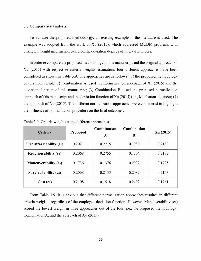
66
3.5 Comparative analysis
To validate the proposed methodology, an existing example in the literature is used. The
example was adopted from the work of Xu (2015), which addressed MCDM problems with
unknown weight information based on the deviation degrees of interval numbers.
In order to compare the proposed methodology in this manuscript and the original approach of
Xu (2015) with respect to criteria weights estimation, four different approaches have been
considered as shown in Table 3.9. The approaches are as follows: (1) the proposed methodology
of this manuscript; (2) Combination A: used the normalization approach of Xu (2015) and the
deviation function of this manuscript; (3) Combination B: used the proposed normalization
approach of this manuscript and the deviation function of Xu (2015) (i.e., Manhattan distance); (4)
the approach of Xu (2015). The different normalization approaches were considered to highlight
the influence of normalization procedure on the final outcomes.
Table 3.9: Criteria weights using different approaches
Criteria Proposed Combination
A
Combination
B Xu (2015)
Fire attack ability (c1) 0.2021 0.2215 0.1980 0.2189
Reaction ability (c2) 0.2068 0.2755 0.1504 0.2182
Maneuverability (c3) 0.1736 0.1376 0.2032 0.1725
Survival ability (c4) 0.2068 0.2135 0.2082 0.2143
Cost (c5) 0.2108 0.1518 0.2402 0.1761
From Table 3.9, it is obvious that different normalization approaches resulted in different
criteria weights, regardless of the employed deviation function. However, Maneuverability (c3)
scored the lowest weight in three approaches out of the four, i.e., the proposed methodology,
Combination A, and the approach of Xu (2015).

67
When it comes to deviation degrees consideration, by using the proposed deviation function in
this manuscript, regardless of the normalization approach, Reaction ability (c2) scored the highest
weight and Maneuverability (c3) scored the lowest weight.
To compare the final ranking order of the proposed methodology with the results of Xu (2015),
criteria weights of the proposed approach are used. Consequently, the ranking order of the given
decision problem based on the proposed methodology would be
𝐴1 ≻ 𝐴4 ≻ 𝐴3 ≻ 𝐴2
with 𝐴1 as the best option, which is the best option while using the approach of Xu (2015) as well.
However, the ranking order is different for the rest of alternatives due to procedure differences in
addressing the problem, which can be summarized in the following: (1) Normalization approach;
(2) Deviation function to estimate criteria weights; (3) Alternatives evaluation and ranking
methodology.
It is noteworthy to mention that during the analysis of different possible scenarios for the
deviation between two interval numbers, one scenario was identified where the deviation function
of Xu (2015) (i.e. Manhattan distance) fails to address. The scenario can be denoted by the empty
intersection scenario; which indicates that a given two data points have no points in common.
However, the proposed approach in this manuscript considers this scenario. As a result, Theorem
3.6 is introduced.
Theorem 3.6 For a given two interval numbers 𝑎 = [𝑎, 𝑎] and 𝑏 = [𝑏, 𝑏], where the intersection
between the two data points is empty (i.e. 𝑎 ≻ 𝑏 𝑜𝑟 𝑏 ≻ 𝑎), the deviation between the two data
points cannot be determined using the Manhattan distance.
Proof 3.6 The distance between two numbers 𝑎 𝑎𝑛𝑑 𝑏 on a number line is given by the absolute
value of their difference, that is |(𝑎 − 𝑏)| = |(𝑏 − 𝑎)| (Cohen et al., 2011), by the same token the
difference between two interval numbers 𝑎 = [𝑎, 𝑎] and 𝑏 = [𝑏, 𝑏] on a number line, where 𝑎 ≻
𝑎 ≻ 𝑏 ≻ 𝑏, can be given as follows:

68
𝑑(𝑎, 𝑏) = |(𝑎 − 𝑎)| + |(𝑎 − 𝑏)| + |(𝑏 − 𝑏)| (3.40)
Considering the ordering of the normalized grey numbers (𝑎 ≻ 𝑎 ≻ 𝑏 ≻ 𝑏), Eq. (3.40) would be
𝑑(𝑎, 𝑏) = (�̃� − �̃�) + (�̃� − �̃�) + (�̃� − �̃�) (3.41)
By applying basic arithmetic operations, Eq. (3.41) can be written as
𝑑(𝑎, 𝑏) = (�̃� − �̃�) ≠ |(�̃� − �̃�)| + |(�̃� − �̃�)| (3.42)
Accordingly, the deviation function by Xu (2015) fails to address the deviation between two
interval numbers in which they have no data points in common. In contrast, the proposed deviation
algorithm (i.e., Algorithm 3.2) in this thesis considers this case.
3.6 Conclusion
Although MCDM problems with unknown weight information have been addressed in the
literature using different approaches and different types of information (e.g., fuzzy set theory,
intuitionistic fuzzy set, hesitant fuzzy set, interval fuzzy set, neutrosophic set), there exist MCDM
problems with small amount of data and poor information, which cannot be described by a
probability distribution. In such MCDM problems, the applicability of existing approaches would
be influenced. To overcome this limitation, this manuscript investigates MCDM problems with
small amount of data and poor information, where information on criteria weights is completely
unknown, and proposes to use grey systems theory due to its less restricted procedure that neither
requires any robust membership function, nor a probability distribution. To this end, a new hybrid
MCDM methodology is proposed. At first, the unknown criteria weights should be estimated.
Accordingly, a new optimization model is established based on the integration of grey system
theory’s principles and the maximizing deviation method. By solving the optimization model, a
function to determine the optimal criteria weights is obtained. Consequently, potential alternatives
are evaluated by integrating degrees of possibility and PROMETHEE II, where the resultant
weights are used to evaluate possible alternatives. Once the evaluation process is completed, the

69
rank index for potential alternatives is provided based on the values of global preferences, wherein
the higher the value, the better is the alternative.
To determine the feasibility of the proposed methodology, an illustrative example is given;
whereas to validate the methodology, a comparative analysis with an existing approach is
provided.
The contributions of this manuscript over existing research works can be summarized in the
following points: (1) Determine the optimal criteria weights for MCDM problems with small
amount of data and poor information where information on criteria weights is unknown, by
establishing a new optimization model which integrates the principles of the grey system theory
and the maximizing deviation method; (2) Extend the PROMETHEE II approach such that to
evaluate and rank potential alternatives within uncertain MCDM with unknown weights
information; (3) Generalize the determination procedure of deviation degrees to account for
various scenarios of deviation between interval numbers.
70
Chapter 4
A New Approach to Address Uncertain Dynamic Multi-
Criteria Decision Problems with Unknown Weight
Information
Abstract
Conventional Multi-Criteria Decision Making (MCDM) approaches are not suitable to address the
dynamics over time. Therefore, different hybrid approaches have been introduced to deal with
Dynamic MCDM (DMCDM) problems. Two main concerns with existing approaches were
identified: (1) Criteria weights establishment within the context of DMCDM with unknown weight
information; (2) Weight vector establishment of different periods where the influences of the
evaluation criteria are changing over time. To overcome the shortcomings of existing approaches,
this manuscript proposed a new hybrid methodology to handle DMCDM with small amount of
data and poor information, which cannot be described by a probability distribution, where
information on criteria weights and the influence of different time periods are unknown. The
proposed methodology estimates the unknown criteria weights using the maximizing deviation
method, where the deviation degrees calculations adopted the principles of grey systems theory.
When it comes to weight vector establishments of different periods, a new optimization model is
introduced where the influence of different evaluation criteria on decision problems are changing
over different periods. To evaluate and rank potential alternatives of DMCDM problems, the
PROMETHEE II approach is extended using the optimized weights and the possibility degrees.
71
4.1 Introduction
Multi-Criteria Decision Making (MCDM) is a branch of operation research that is intended to
aid decision makers in establishing coherent preferences in complex decision problems (Roy,
2016; Wątróbski & Jankowski, 2016). Different methods of MCDM have been proposed, each of
which has its own characteristics in evaluating decision problems (Mardani et al., 2015).
Therefore, understanding the background differences among these methods is essential to properly
analyze a decision problem. To differentiate between the MCDM methods, the following
classification is provided (Belton & Stewart, 2002):
(1) Value measurement methods: this group of methods are value focused, in which the overall
evaluation over different criteria is used to select between alternatives; among this category of
methods are Analytic Hierarchy Process (AHP), Multi-Attribute Utility Theory (MAUT), and
Weighted Average (WA) approach.
(2) Goal, aspiration, or reference-level methods: this group of methods are optimal value
focused where alternatives are evaluated with respect to a particular goal, aspiration, or
reference levels; examples of methods within this category are: Technique for Order
Preference by Similarity to Ideal Solution (TOPSIS) and Vlsekriterijumska Optimizacijia I
Kompromisno Resenje (VIKOR).
(3) Outranking methods: this group of methods are pairwise comparisons focused where
alternatives are compared over each criterion and the aggregated comparisons would be used
to rank the alternatives; the most prominent methods within this category are: ELimination and
Choice Expressing REality (ELECTRE) and Preference Ranking Organization METHod for
Enrichment Evaluations (PROMETHEE) family of methods.
Although MCDM conventional approaches can be used to establish a better ground for
decision makers in complex decision problems, they are deemed inappropriate to handle decision
problems that involve uncertain, imprecise, and subjective data; as they presume the availability
of precise information.
The complexity of decision problems increases in many real life applications, where
information from different periods (e.g., multi-period investment, medical diagnosis) should be

72
considered in the decision process (G. Wei, 2011). Conventional MCDM approaches are not
appropriate to understand the dynamics over time, as they are clearly static (Pruyt, 2007).
4.2 Background
To account for the dynamic aspects in MCDM problems, different hybrid approaches have
been proposed. For instance, Lin et al. (2008) developed a DMCDM method using a hybrid
approach, in which TOPSIS was used as the main structure, while the combination of grey concept
(which was introduced by Ju-long (1982) to handle data imprecision or insufficiency using interval
number where its exact value is unknown but a range within which the value lies is known (Sifeng
Liu & Lin, 2006)) and Minkowski distance function (which is a generalization function of the most
widely used distance measures (i.e., Euclidean distance and the Manhattan distance) between two
data points (Chen, 2018)) to handle uncertain information and the multi period evaluations. Park,
Cho, and Kwun (2013) proposed two aggregation operators called Dynamic Intuitionistic Fuzzy
Weighted Geometric (DIFWG) operator and Uncertain Dynamic Intuitionistic Fuzzy Weighted
Geometric (UDIFWG) operator to solve MCDM problems under dynamic intuitionistic fuzzy
environment using VIKOR principles; in which the evaluations are expressed in different periods
using intuitionistic fuzzy set, which is an extension of Zadeh’s fuzzy set whose basic component
is only a membership function for an element to a given set, in which the intuitionistic fuzzy set
defines the degree of membership as well as the degree of non-membership. Gümüş and Bali
(2017) introduced two methods based on Einstein operational laws on intuitionistic fuzzy sets,
which are Dynamic Intuitionistic Fuzzy Einstein Averaging (DIFWA∊) operator and Dynamic
Intuitionistic Fuzzy Einstein Geometric Averaging (DIFWG∊) operator, to solve multi-periods
MCDM problems within intuitionistic fuzzy environment. Esangbedo and Che (2016) proposed a
Grey Weighted Sum Model (GWSM) to handle uncertainty over multi-periods multi-criteria
decision problems, in which interval grey numbers are used to express varying performances over
multi-periods, while the concept of WSM is used to aggregate the results of different alternatives.
Wei and Lin (2008) proposed a new concept of dynamic uncertain multiplicative linguistic
preference relations to solve the multi-periods MCDM problems, where the criteria values are
given in uncertain multiplicative linguistic relations collected in different time periods.

73
A common concern of the above-mentioned approaches is related to the weight vector
establishment for different periods. The weights of different periods are assumed to be given or
simply ignored. Moreover, information on criteria weights is assumed to be known.
To account for the weights of different time periods in MCDM problems, different studies used
the Basic Unit-interval Monotonic (BUM) function (Yager, 1998, 2004), which is one of the most
common weight determination methods of different time periods. For instance, Peng and Wang
(2014) presented some dynamic hesitant fuzzy aggregation operators, based on the weighted
averaging and the weighted geometric approaches, to tackle multi-period decision making
problems where all decision information from different period is provided in hesitant fuzzy
information (which has been introduced by Torra (2010) as an extension of fuzzy set where the
membership of an element to a given set can be denoted by an interval in order to deal with
uncertain information). However, two linguistic approaches were introduced based on BUM
function to estimate the weight vector of the different periods: one approach depends on the degree
of emphasis between the initial and the final period; while the other focuses on the values of the
argument variables at each period, which is determined based on the score function of Xia and Xu
(2011). Similarly, G. Li et al. (2015) proposed a dynamic fuzzy multiple criteria decision making
(DFMCDM) method based on TOPSIS, where the time weight is calculated using BUM function.
Within the context of DMCDM problems under uncertain environment, existing methods to
obtain the weights of different time periods, such as BUM function, would address the influence
of different periods independently from the evaluation criteria. In other word, the variabilities in
nature of different decision criteria are ignored, which impose a falsify assumption with regards to
the dynamic aspect of this type of MCDM problems. Furthermore, the overall evaluation of a
MCDM problem is based on alternatives evaluations over the multi-criteria and the weights of the
criteria. The above-mentioned approaches assume that information about criteria weights is
known. However, in cases where the criteria weights are unknown due to different reasons, e.g.,
time pressure, limited expertise, incomplete knowledge, and lack of information (Das et al., 2016;
S. Zhang et al., 2011), the overall evaluations cannot be derived (Xu, 2015). Accordingly, the
proper assessment of criteria weights is critical for MCDM problems and may influence the
analysis of a decision problem (Das et al., 2016).
In such decision settings, it is useful to utilize the available information, the knowledge, and
the expertise of the decision makers to approximate evaluation ranges (Lin et al., 2008). To

74
approximate evaluation ranges, Gao and Liu (2016) mentioned that maximizing deviation method
is the most popular approach to establish objective weights for solving MCDM problems with
unknown weight information. The maximizing deviation method introduced by Wang (1998)
where larger deviations are being emphasized more than smaller ones.
Although several research papers have tried to address MCDM problems with unknown
criteria weights using different types of information (e.g., fuzzy set theory, intuitionistic fuzzy set,
and hesitant fuzzy set), there exist decision problems with small amount of data and poor
information, which cannot be described by a probability distribution. In such decision problems,
grey systems theory is recommended (D.-C. Li et al., 2012; S. Liu & Lin, 2006) due to its less
restricted procedure that neither requires any robust membership function, nor a probability
distribution (Memon et al., 2015).
Building on the above arguments, the aim of this manuscript is to contribute to the current
literature by addressing DMCDM problems with small amount of data and poor information where
information on criteria weights and the weight vector of different time periods are unknown. To
this end, a new hybrid DMCDM methods is proposed using the principles of grey systems theory,
the maximizing deviation method, possibility degrees, and PROMETHEE II.
This manuscript is organized as follows: section 4.3 establishes the proposed approach to
handle Dynamic Grey Multi-Criteria Decision Making (DGMCDM) problems; section 4.4 reflects
the feasibility and the practicability of the proposed approach using an adopted case; section 4.5
provides a comparative analysis with existing approaches to validate the proposed approach;
finally, section 4.6 provides the concluding remarks.
4.3 Decision making method of DGMCDM with unknown weight information
4.3.1 Problem description
Definition 4.1 Let 𝐴 = {𝐴1, 𝐴2 … , 𝐴𝑛} denote the set of available alternatives of a multi-periods-
multi-criteria decision making, where 𝑛 is the number of the alternatives and 𝑖 = 1, 2… , 𝑛. Let
𝐶 = {𝑐1, 𝑐2 … , 𝑐𝑚} represent the set of evaluation criteria, where m is the number of criteria
and 𝑗 = 1, 2… ,𝑚 . Let 𝑆(𝑡) = {𝑡1 , 𝑡2 … , 𝑡𝑝} indicate the set of time periods, where 𝑝 is the
number of different periods and 𝑘 = 1, 2… , 𝑝.

75
Definition 4.2 Let 𝐴 × 𝐶 × 𝑆(𝑡) be the Cartesian product of the set of alternatives, the set of
criteria, and the set of periods. Let 𝑅 [⨂] denote the set of interval grey numbers, in which each
element of 𝑅 [⨂] represent an evaluation of 𝐴𝑖 over 𝑐𝑗 within 𝑡𝑘 and denoted by an interval grey
number 𝑦𝑖𝑗𝑘(⨂) ∈ [𝑦𝑖𝑗𝑘, 𝑦𝑖𝑗𝑘], where 0 ≤ 𝑦𝑖𝑗𝑘 ≤ 𝑦𝑖𝑗𝑘
. Accordingly, the grey description function
for a decision matrix (𝑓⨂) within a DGMCDM problem is defined as follows:
𝑓⨂: 𝐴 × 𝐶 × 𝑆(𝑡) → 𝑅[⨂], 𝑡ℎ𝑢𝑠 (4.1)
∀𝑓⨂(𝐴𝑖 ∈ 𝐴, 𝑐𝑗 ∈ 𝐶, 𝑡𝑘 ∈ 𝑆(𝑡)): 𝑦𝑖𝑗𝑘(⨂) ∈ 𝑅[⨂]
Definition 4.3 Assume that the influence of 𝑐𝑗 ∈ 𝐶 (𝑗 = 1, 2… ,𝑚) on a decision problem is
changing over 𝑡𝑘 (𝑘 = 1, 2… , 𝑝). Let the weight of 𝑐𝑗 over 𝑡𝑘 be denoted by 𝑤𝑗𝑘, where 𝑤𝑗𝑘 ∈
[0,1] and ∑ 𝑤𝑗𝑘𝑚𝑗=1 = 1; but the information on criteria weights is unknown.
Definition 4.4 Let 𝜃𝑗 = {𝜃𝑗 (𝑡1), 𝜃𝑗 (𝑡2)… , 𝜃𝑗 (𝑡𝑝)} (𝑗 = 1, 2… ,𝑚) denote the weight vector of
𝑆(𝑡) = {𝑡1 , 𝑡2 … , 𝑡𝑝} with respect to 𝑐𝑗, where 𝜃𝑗 (𝑡𝑘) ∈ [0,1] and ∑ 𝜃𝑗 (𝑡𝑘)𝑝𝑘=1 = 1 (𝑘 =
1, 2… , 𝑝); but the information on 𝜃𝑗 is unknown.
4.3.2 Normalize DGMCDM
For consistency in the evaluations over each period such that all the evaluations would be grey
based with [0,0] ≤ 𝑦𝑖𝑗𝑘(⨂) ≤ [1,1] (Bai et al., 2012), a normalization procedure of two steps is
used over each decision matrix: first, turn all non-grey values (e.g., crisp number, which is a single
precise number) in the decision matrix into interval grey numbers according to Definition 4.5;
second, normalize all the values using Algorithm 4.1, which is explained by Definition 4.6.
Definition 4.5 Let 𝑦𝑖𝑗 denote a white number that represents the evaluation of alternative 𝐴𝑖 (𝑖 =
1, 2… , 𝑛) over criterion 𝑐𝑗 (𝑗 = 1, 2… ,𝑚) within a given period 𝑡𝑘 (𝑘 = 1, 2… , 𝑝) such that, the
relative grey number (𝑦𝑖𝑗𝑘(⨂)) of the given white number (𝑦𝑖𝑗𝑘) is
𝑦𝑖𝑗𝑘(⨂) = [𝑦𝑖𝑗𝑘, 𝑦𝑖𝑗𝑘] , where 𝑦𝑖𝑗𝑘 = 𝑦𝑖𝑗𝑘 = 𝑦𝑖𝑗𝑘 (4.2)
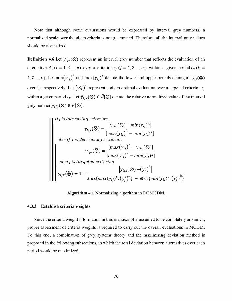
76
Note that although some evaluations would be expressed by interval grey numbers, a
normalized scale over the given criteria is not guaranteed. Therefore, all the interval grey values
should be normalized.
Definition 4.6 Let 𝑦𝑖𝑗𝑘(⨂) represent an interval grey number that reflects the evaluation of an
alternative 𝐴𝑖 (𝑖 = 1, 2… , 𝑛) over a criterion 𝑐𝑗 (𝑗 = 1, 2… ,𝑚) within a given period 𝑡𝑘 (𝑘 =
1, 2… , 𝑝). Let min(𝑦𝑖𝑗)𝑘 and max(𝑦𝑖𝑗)
𝑘 denote the lower and upper bounds among all 𝑦𝑖𝑗(⨂)
over 𝑡𝑘 , respectively. Let (𝑦𝑗𝑘∗ )
𝑘 represent a given optimal evaluation over a targeted criterion 𝑐𝑗
within a given period 𝑡𝑘. Let �̃�𝑖𝑗𝑘(⨂) ∈ �̃�[⨂] denote the relative normalized value of the interval
grey number 𝑦𝑖𝑗𝑘(⨂) ∈ 𝑅[⊗].
|
|
|
|
|
|
|
|
|
|
|
|
𝑖𝑓𝑗 𝑖𝑠 𝑖𝑛𝑐𝑟𝑒𝑎𝑠𝑖𝑛𝑔 𝑐𝑟𝑖𝑡𝑒𝑟𝑖𝑜𝑛
|
|
|𝑦𝑖𝑗𝑘(⨂̃) =
[𝑦𝑖𝑗𝑘(⊗)−𝑚𝑖𝑛(𝑦𝑖𝑗)𝑘]
[𝑚𝑎𝑥(𝑦𝑖𝑗)𝑘−𝑚𝑖𝑛(𝑦𝑖𝑗)𝑘]
𝑒𝑙𝑠𝑒 𝑖𝑓 𝑗 𝑖𝑠 𝑑𝑒𝑐𝑟𝑒𝑎𝑠𝑖𝑛𝑔 𝑐𝑟𝑖𝑡𝑒𝑟𝑖𝑜𝑛
|
|𝑦𝑖𝑗𝑘(⨂̃) =
[𝑚𝑎𝑥(𝑦𝑖𝑗)𝑘− 𝑦𝑖𝑗𝑘(⊗)]
[𝑚𝑎𝑥(𝑦𝑖𝑗)𝑘−𝑚𝑖𝑛(𝑦𝑖𝑗)𝑘]
𝑒𝑙𝑠𝑒 𝑗 𝑖𝑠 𝑡𝑎𝑟𝑔𝑒𝑡𝑒𝑑 𝑐𝑟𝑖𝑡𝑒𝑟𝑖𝑜𝑛
|𝑦𝑖𝑗𝑘(⨂̃) = 1 −|𝑦𝑖𝑗𝑘(⊗)−(𝑦𝑗
∗)𝑘|
𝑀𝑎𝑥{𝑚𝑎𝑥(𝑦𝑖𝑗)𝑘, (𝑦𝑗∗)𝑘} − 𝑀𝑖𝑛 {𝑚𝑖𝑛(𝑦𝑖𝑗)𝑘, (𝑦𝑗
∗)𝑘}
Algorithm 4.1 Normalizing algorithm in DGMCDM.
4.3.3 Establish criteria weights
Since the criteria weight information in this manuscript is assumed to be completely unknown,
proper assessment of criteria weights is required to carry out the overall evaluations in MCDM.
To this end, a combination of grey systems theory and the maximizing deviation method is
proposed in the following subsections, in which the total deviation between alternatives over each
period would be maximized.

77
4.3.3.1 Construct deviation matrix
As mentioned earlier, the maximizing deviation method considers criteria with larger
deviations more than criteria with smaller deviations. Accordingly, deviation measures between
normalized interval grey evaluations over a given period can be established using Algorithm 4.2,
which is explained by Definition 4.7.
Definition 4.7 Let the deviation measure between the normalized grey evaluations of two
alternatives over a criterion 𝑐𝑗 within a period 𝑡𝑘 be denoted by 𝑑(�̃�𝑖𝑗𝑘(⨂), �̃�ℎ𝑗𝑘(⨂)),
where 𝑖, ℎ = 1, 2… , 𝑛; 𝑗 = 1, 2… ,𝑚 and 𝑘 = 1, 2… , 𝑝.
|
|
|
|
𝑖𝑓 �̃�𝑖𝑗𝑘(⨂) = �̃�ℎ𝑗𝑘(⨂)
|
|
|
𝑑(�̃�𝑖𝑗𝑘(⨂), �̃�ℎ𝑗𝑘(⨂) ) = 0
𝑒𝑙𝑠𝑒 𝑖𝑓 �̃�𝑖𝑗𝑘(⨂) ≠ �̃�ℎ𝑗𝑘(⨂) ∧ (�̃�𝑖𝑗𝑘 ≽ �̃�ℎ𝑗𝑘)
|
|
𝑑(�̃�𝑖𝑗𝑘(⨂), �̃�ℎ𝑗𝑘(⨂) ) = (�̃�𝑖𝑗𝑘 − �̃�ℎ𝑗𝑘)
𝑒𝑙𝑠𝑒 𝑖𝑓�̃�𝑖𝑗𝑘≻ �̃�
ℎ𝑗𝑘≻ �̃�ℎ𝑗𝑘 ≻ �̃�𝑖𝑗𝑘
|
𝑑(�̃�𝑖𝑗𝑘(⨂), �̃�ℎ𝑗𝑘(⨂) ) = |(�̃�𝑖𝑗𝑘 + �̃�ℎ𝑗𝑘) − (�̃�𝑖𝑗𝑘 + �̃�ℎ𝑗𝑘)|
𝑒𝑙𝑠𝑒
𝑑(�̃�𝑖𝑗𝑘(⨂), �̃�ℎ𝑗𝑘(⨂) ) = |(�̃�𝑖𝑗𝑘 − �̃�ℎ𝑗𝑘) + (�̃�𝑖𝑗𝑘 − �̃�ℎ𝑗𝑘)|
Algorithm 4.2: Deviation measure algorithm in DGMCDM.
4.3.3.2 Estimate criteria weights
Definition 4.8 Let 𝐷𝑖𝑗𝑘(𝑤) denote the overall deviation between alternative 𝐴𝑖 and other
alternatives over a criterion 𝑐𝑗 within a period 𝑡𝑘 . Let 𝑤𝑗𝑘 denote the associated criterion weight
within 𝑡𝑘 such that,
𝐷𝑖𝑗𝑘(𝑤) = ∑ 𝑑(�̃�𝑖𝑗𝑘(⨂) , �̃�ℎ𝑗𝑘(⨂) )𝑤𝑗𝑘𝑛ℎ=1,ℎ≠𝑖
, (4.3)
𝑖 = 1, 2… , 𝑛; 𝑗 = 1, 2… ,𝑚; 𝑘 = 1, 2… , 𝑝
Definition 4.9 Let 𝐷𝑗𝑘(𝑤) denote the global deviation between alternatives over 𝑐𝑗 within 𝑡𝑘 , such
that

78
𝐷𝑗𝑘(𝑤) = ∑ 𝐷𝑖𝑗𝑘(𝑤)𝑛𝑖=1 = ∑ ∑ 𝑑(�̃�𝑖𝑗𝑘(⨂) , �̃�ℎ𝑗𝑘(⨂) )𝑤𝑗𝑘
𝑛ℎ=1,ℎ≠𝑖
𝑛𝑖=1 , (4.4)
𝑗 = 1, 2… ,𝑚; 𝑘 = 1, 2… , 𝑝
Definition 4.10 Let 𝐷𝑘(𝑤) denote the total deviations over all the criteria within 𝑡𝑘, in which the
total deviation function over 𝑡𝑘 is expressed as follows:
𝐷𝑘(𝑤) = ∑ 𝐷𝑗𝑘(𝑤)𝑚𝑗=1 = ∑ ∑ ∑ 𝑑(�̃�𝑖𝑗𝑘(⨂) , �̃�ℎ𝑗𝑘(⨂) )𝑤𝑗𝑘
𝑛ℎ=1,ℎ≠𝑖
𝑛𝑖=1
𝑚𝑗=1 , (4.5)
𝑘 = 1, 2… , 𝑝
Theorem 4.1 In DGMCDM problems with unknown criteria weights, the optimal criteria weights
𝑤𝑗𝑘∗ = (𝑤1𝑘
∗ , 𝑤2𝑘∗ … ,𝑤𝑚𝑘
∗ ) which maximize the total deviation between alternatives over each
period 𝑡𝑘 can be obtained as follows:
𝑤𝑗𝑘∗ =
∑ ∑ 𝑑(�̃�𝑖𝑗𝑘(⨂),�̃�ℎ𝑗𝑘(⨂) )𝑛ℎ=1,ℎ≠𝑖
𝑛𝑖=1
√∑ [∑ ∑ 𝑑(�̃�𝑖𝑗𝑘(⨂),�̃�ℎ𝑗𝑘(⨂) )𝑛ℎ=1,ℎ≠𝑖
𝑛𝑖=1 ]
2
𝑚𝑗=1
, (4.6)
𝑗 = 1,2… ,𝑚; 𝑘 = 1, 2… , 𝑝
In order to satisfy the normalization constraint condition, the weight of criteria 𝑐𝑗 within a
period 𝑡𝑘 can be determined as follows:
𝑤𝑗𝑘 =𝑤𝑗𝑘∗
∑ 𝑤𝑗𝑘∗𝑚
𝑗=1
=
∑ ∑ 𝑑(�̃�𝑖𝑗𝑘(⨂),�̃�ℎ𝑗𝑘(⨂) )𝑛ℎ=1,ℎ≠𝑖
𝑛𝑖=1
∑ ∑ ∑ 𝑑(�̃�𝑖𝑗𝑘(⨂),�̃�ℎ𝑗𝑘(⨂) )𝑛ℎ=1,ℎ≠𝑖
𝑛𝑖=1
𝑚𝑗=1
(4.7)
Proof 4.1 For unknown criteria weights, the maximizing deviation method (Y. M. Wang, 1998)
can be adapted, in which the criteria weights over a period 𝑡𝑘 are being estimated based on the
deviation degrees between the evaluations within 𝑡𝑘. To this end, the following optimization model
is established

79
𝑚𝑎𝑥𝐷𝑘(𝑤) = ∑ 𝐷𝑗𝑘(𝑤)𝑚𝑗=1 = ∑ ∑ ∑ 𝑑(�̃�𝑖𝑗𝑘(⨂) , �̃�ℎ𝑗𝑘(⨂) )𝑤𝑗𝑘
∗𝑛ℎ=1,ℎ≠𝑖
𝑛𝑖=1
𝑚𝑗=1 (4.8)
𝑠. 𝑡. ∑ (𝑤𝑗𝑘∗ )
2= 1𝑚
𝑗=1 , 𝑤𝑗𝑘∗ ≥ 0, (4.9)
𝑗 = 1,2… ,𝑚; 𝑘 = 1, 2… , 𝑝
Note that ∑ (𝑤𝑗𝑘∗ )
2= 1𝑚
𝑗=1 is used as a constraint to accentuate the larger deviations within each
time period. Thus, to ensure that criteria which make larger deviations would be assigned higher
weights in comparison to criteria which make smaller deviations.
The model can be solved using Lagrange function (Z. Xu & Cai, 2012):
𝐿(𝑤𝑗𝑘∗ , 𝜆) = 𝐷𝑘(𝑤) −
1
2𝜆 (∑ (𝑤𝑗𝑘
∗ )2− 1𝑚
𝑗=1 ), where (4.10)
𝜆 is the Lagrange multiplier. Thus,
𝐿(𝑤𝑗𝑘∗ , 𝜆) = ∑ ∑ ∑ 𝑑(�̃�𝑖𝑗𝑘(⨂) , �̃�ℎ𝑗𝑘(⨂) )𝑤𝑗𝑘
∗𝑛ℎ=1,ℎ≠𝑖
𝑛𝑖=1
𝑚𝑗=1 −
1
2𝜆 (∑ (𝑤𝑗𝑘
∗ )2− 1𝑚
𝑗=1 ) (4.11)
By calculating the partial derivative of Eq. (4.11) with respect to 𝑤𝑗𝑘∗ (𝑗 = 1, 2… ,𝑚, 𝑘 =
1, 2… , 𝑝) and 𝜆, while setting these partial derivatives to zero, the following equations are
obtained:
𝜕𝐿(𝑤𝑗𝑘
∗ ,𝜆)
𝜕𝑤𝑗𝑘∗ = ∑ ∑ 𝑑(�̃�𝑖𝑗𝑘(⨂), �̃�ℎ𝑗𝑘(⨂) )
𝑛ℎ=1,ℎ≠𝑖
𝑛𝑖=1 − 𝜆𝑤𝑗𝑘
∗ = 0 (4.12)
𝜕𝐿(𝑤𝑗𝑘
∗ ,𝜆)
𝜕𝜆= ∑ (𝑤𝑗𝑘
∗ )2− 1𝑚
𝑗=1 = 0 (4.13)
From Eq. (4.12), we can obtain
𝑤𝑗𝑘∗ =
∑ ∑ 𝑑(�̃�𝑖𝑗𝑘(⨂),�̃�ℎ𝑗𝑘(⨂) )𝑛ℎ=1,ℎ≠𝑖
𝑛𝑖=1
𝜆 (4.14)

80
Since ∑ (𝑤𝑗𝑘∗ )
2= 1𝑚
𝑗=1 , the value of 𝜆 can be obtained using Eq. (4.14) as follows:
∑ (
∑ ∑ 𝑑(�̃�𝑖𝑗𝑘(⨂),�̃�ℎ𝑗𝑘(⨂) )𝑛ℎ=1,ℎ≠𝑖
𝑛𝑖=1
𝜆)
2
= 1𝑚𝑗=1 (4.15)
By simplifying Eq. (4.15)
𝜆 = √∑ [∑ ∑ 𝑑(�̃�𝑖𝑗𝑘(⨂), �̃�ℎ𝑗𝑘(⨂) )𝑛ℎ=1,ℎ≠𝑖
𝑛𝑖=1 ]
2
𝑚𝑗=1 (4.16)
Thus, the optimal solution of the model is
𝑤𝑗𝑘∗ =
∑ ∑ 𝑑(�̃�𝑖𝑗𝑘(⨂),�̃�ℎ𝑗𝑘(⨂) )𝑛ℎ=1,ℎ≠𝑖
𝑛𝑖=1
√∑ [∑ ∑ 𝑑(�̃�𝑖𝑗𝑘(⨂),�̃�ℎ𝑗𝑘(⨂) )𝑛ℎ=1,ℎ≠𝑖
𝑛𝑖=1 ]
2
𝑚𝑗=1
, 𝑗 = 1, 2… ,𝑚; 𝑘 = 1, 2… , 𝑝
4.3.4 Estimate the influence of dynamic evaluations
Since weight information of different time periods is unknown, the overall evaluation over a
DGMCDM problem cannot be obtained. As a result, the weight of the different time periods with
respect to each criterion should be established. To this end, a new optimization model is proposed,
in which the evaluation space over a DGMCDM problem would be maximized.
Theorem 4.2 In a DGMCDM where the weight information of different time periods is unknown,
the optimal solution to maximize the evaluation space over the dynamic decision problem can be
obtained using 𝜃𝑗 = {𝜃𝑗 (𝑡1), 𝜃𝑗 (𝑡2)… , 𝜃𝑗 (𝑡𝑝)}, where
𝜃𝑗 (𝑡𝑘)∗ =
∑ ∑ 𝑑(�̃�𝑖𝑗𝑘(⨂),�̃�ℎ𝑗𝑘(⨂) )𝑛ℎ=1,ℎ≠𝑖
𝑛𝑖=1
∑ ∑ ∑ 𝑑(�̃�𝑖𝑗𝑘(⨂),�̃�ℎ𝑗𝑘(⨂) )𝑛ℎ=1,ℎ≠𝑖
𝑛𝑖=1
𝑚𝑗=1
√∑
[
∑ ∑ 𝑑(�̃�𝑖𝑗𝑘(⨂),�̃�ℎ𝑗𝑘(⨂) )𝑛ℎ=1,ℎ≠𝑖
𝑛𝑖=1
∑ ∑ ∑ 𝑑(�̃�𝑖𝑗𝑘(⨂),�̃�ℎ𝑗𝑘(⨂) )𝑛ℎ=1,ℎ≠𝑖
𝑛𝑖=1
𝑚𝑗=1
]
𝑝𝑘=1
2, 𝑗 = 1, 2… ,𝑚; 𝑘 = 1, 2… , 𝑝 (4.17)

81
In order to satisfy the normalization constraint condition, the optimal weight of period 𝑡𝑘 with
respect to 𝑐𝑗 can be expressed as
𝜃𝑗 (𝑡𝑘) =𝜃𝑗 (𝑡𝑘)
∗
∑ 𝜃𝑗 (𝑡𝑘)∗𝑝
𝑘=1
=
∑ ∑ 𝑑(�̃�𝑖𝑗𝑘(⨂),�̃�ℎ𝑗𝑘(⨂) )𝑛ℎ=1,ℎ≠𝑖
𝑛𝑖=1
∑ ∑ ∑ 𝑑(�̃�𝑖𝑗𝑘(⨂),�̃�ℎ𝑗𝑘(⨂) )𝑛ℎ=1,ℎ≠𝑖
𝑛𝑖=1
𝑚𝑗=1
∑
[
∑ ∑ 𝑑(�̃�𝑖𝑗𝑘(⨂),�̃�ℎ𝑗𝑘(⨂) )𝑛ℎ=1,ℎ≠𝑖
𝑛𝑖=1
∑ ∑ ∑ 𝑑(�̃�𝑖𝑗𝑘(⨂),�̃�ℎ𝑗𝑘(⨂) )𝑛ℎ=1,ℎ≠𝑖
𝑛𝑖=1
𝑚𝑗=1
]
𝑝𝑘=1
(4.18)
Proof 4.2 In DMCDM problems, if the influence of 𝑐𝑗 ∈ 𝐶 is the same over 𝑡𝑘 ∈ 𝑆(𝑡), for all 𝑗 =
1, 2… ,𝑚 and 𝑘 = 1, 2… , 𝑝, then
𝑤𝑗𝑘 = ∑ 𝜃𝑗 (𝑡𝑘)𝑤𝑗𝑘𝑝𝑘=1 , for all 𝑗 = 1, 2… ,𝑚 and 𝑘 = 1, 2… , 𝑝 (4.19)
However, Eq. (4.19) does not generally hold, i.e., the influence of 𝑐𝑗 is changing over 𝑡𝑘 and thus,
there is always a difference in the value of 𝑤𝑗𝑘. Consequently, a general deviation function 𝐹(𝑒𝑗𝑘)
is introduced:
𝐹(𝑒𝑗𝑘) = (∑ 𝜃𝑗 (𝑡𝑘)∗𝑤𝑗𝑘
𝑝𝑘=1 − 𝑤𝑗𝑘), for all 𝑗 = 1, 2… ,𝑚 and 𝑘 = 1, 2… , 𝑝 (4.20)
Accordingly, to estimate the weight vector 𝜃𝑗 = {𝜃𝑗 (𝑡1), 𝜃𝑗 (𝑡2)… , 𝜃𝑗 (𝑡𝑝)} for 𝑐𝑗, the following
optimization model is constructed by adapting the maximizing deviation method:
𝑚𝑎𝑥 𝐹(𝑒𝑗𝑘) = (∑ 𝜃𝑗 (𝑡𝑘)∗𝑤𝑗𝑘
𝑝𝑘=1 − 𝑤𝑗𝑘) (4.21)
𝑠. 𝑡. ∑ (𝜃𝑗 (𝑡𝑘)∗)2= 1𝑝
𝑘=1 , 𝜃𝑗 (𝑡𝑘) ∈ [0,1], 𝑗 = 1,2… ,𝑚, 𝑘 = 1, 2… , 𝑝 (4.22)
Note that ∑ (𝜃𝑗 (𝑡𝑘)∗)2= 1𝑝
𝑘=1 is used as a constraint to stress the larger deviations by reflecting a
wider range, which would maximize the evaluation space.
The model can be solved using Lagrange function:
𝐿(𝜃𝑗 (𝑡𝑘)∗, 𝜆) = 𝐹(𝑒𝑗𝑘) −
1
2𝜆(∑ 𝜃𝑗 (𝑡𝑘)
2 − 1𝑝𝑘=1 ), where (4.23)

82
𝜆 is the Lagrange multiplier. Thus,
𝐿(𝜃𝑗 (𝑡𝑘)∗, 𝜆) = (∑ 𝜃𝑗 (𝑡𝑘)
∗𝑤𝑗𝑘𝑝𝑘=1 − 𝑤𝑗𝑘) −
1
2𝜆 (∑ (𝜃𝑗 (𝑡𝑘)
∗)2− 1𝑝
𝑘=1 ) (4.24)
By calculating the partial derivative of Eq. (4.24) with respect to 𝜃𝑗 (𝑡𝑘)∗ (𝑗 = 1, 2… ,𝑚, 𝑘 =
1, 2… , 𝑝) and 𝜆, while setting these partial derivatives to zero, the following equations are
obtained:
𝜕𝐿(𝜃𝑗 (𝑡𝑘)
∗,𝜆)
𝜕𝜃𝑗 (𝑡𝑘)∗ = 𝑤𝑗𝑘 − 𝜆𝜃𝑗 (𝑡𝑘)
∗ = 0 (4.25)
𝜕𝐿(𝜃𝑗 (𝑡𝑘)
∗,𝜆)
𝜕𝜆= ∑ ∑ (𝜃𝑗 (𝑡𝑘)
∗)2− 1𝑝
𝑘=1𝑝𝑘=1 = 0 (4.26)
From Eq. (4.25), we can obtain
𝜃𝑗 (𝑡𝑘)∗ =
𝑤𝑗𝑘
𝜆 (4.27)
Since ∑ (𝜃𝑗 (𝑡𝑘)∗)2= 1𝑝
𝑘=1 , the value of 𝜆 can be obtained using Eq. (4.27) as follows:
∑ (𝑤𝑗𝑘
𝜆)2
= 1𝑝𝑘=1 (4.28)
By simplifying Eq. (4.28)
𝜆 = √∑ [𝑤𝑗𝑘]2𝑝
𝑘=1 (4.29)
Thus, the optimal solution of the model is
𝜃𝑗 (𝑡𝑘)∗ =
𝑤𝑗𝑘
√∑ [𝑤𝑗𝑘]2𝑝
𝑘=1
=
∑ ∑ 𝑑(�̃�𝑖𝑗𝑘(⨂),�̃�ℎ𝑗𝑘(⨂) )𝑛ℎ=1,ℎ≠𝑖
𝑛𝑖=1
∑ ∑ ∑ 𝑑(�̃�𝑖𝑗𝑘(⨂),�̃�ℎ𝑗𝑘(⨂) )𝑛ℎ=1,ℎ≠𝑖
𝑛𝑖=1
𝑚𝑗=1
√∑
[
∑ ∑ 𝑑(�̃�𝑖𝑗𝑘(⨂),�̃�ℎ𝑗𝑘(⨂) )𝑛ℎ=1,ℎ≠𝑖
𝑛𝑖=1
∑ ∑ ∑ 𝑑(�̃�𝑖𝑗𝑘(⨂),�̃�ℎ𝑗𝑘(⨂) )𝑛ℎ=1,ℎ≠𝑖
𝑛𝑖=1
𝑚𝑗=1
]
𝑝𝑘=1
2

83
4.3.5 Evaluate and rank feasible alternatives
Once criteria weights are established and the dynamism over the multi-criteria decision
problem has been considered, the DGMCDM problem would be evaluated by extending the
PROMETHEE II approach using the optimized weights and the possibility degrees. The detailed
procedure of evaluating and ranking decision alternatives is provided in the rest of this section.
4.3.5.1 Establish preferences
To establish preferences among available alternatives over each criterion within a given
period 𝑡𝑘, the possibility degree formula is used based on the definition of Xu and Da (2002).
Definition 4.11 Let 𝑙 �̃�𝑗𝑘(⨂) and 𝑙 �̃�𝑗𝑘(⨂) denote the difference between the upper and lower limits
of two normalized grey numbers �̃�(⨂) and �̃�(⨂), respectively, over a criterion 𝑐𝑗 within a
period 𝑡𝑘 such that,
𝑙 �̃�𝑗𝑘(⨂) = �̃�𝑗𝑘 − �̃�𝑗𝑘 (4.30)
𝑙�̃�𝑗𝑘(⨂) = �̃�𝑗𝑘 − �̃�𝑗𝑘
Definition 4.12 Let 𝑝𝑗𝑘(�̃�(⨂) ≻ �̃�(⨂)) denote the preference degree of �̃�(⨂) over �̃�(⨂) with
respect to 𝑐𝑗 within 𝑡𝑘, in which 𝑝𝑗𝑘(�̃�(⨂) ≻ �̃�(⨂)) would be determined using the possibility
degree formula as follows:
𝑝𝑗𝑘(�̃�(⨂) ≻ �̃�(⨂)) =�̃�𝑗−�̃�𝑗
𝑙�̃�(⨂)𝑗+𝑙�̃�(⨂)𝑗 (4.31)
Definition 4.13 Let the sum of preferences for any two unequal grey numbers (e.g., �̃�(⨂) =
[�̃�, �̃�] and �̃�(⨂) = [�̃�, �̃�]) equal to 1, such that
𝑝𝑗𝑘(�̃�(⨂), �̃�(⨂)) = 𝑝𝑗𝑘(�̃�(⨂) ≻ �̃�(⨂)) + 𝑝𝑗𝑘(�̃�(⨂) ≻ �̃�(⨂)) = 1 (4.32)
Based on Eqs. (4.31) and (4.32), 𝑝𝑗𝑘(�̃�(⨂) ≻ �̃�(⨂)) would be determined as follows:

84
𝑝𝑗𝑘(�̃�(⨂) ≻ �̃�(⨂)) =
{
0 if 𝑝𝑗𝑘(�̃�(⨂) ≻ �̃�(⨂)) ≤ 0
�̃�𝑗𝑘−�̃�𝑗𝑘
𝑙 �̃�𝑗𝑘(⨂)+𝑙 �̃�𝑗𝑘(⨂)
if 0 < 𝑝𝑗𝑘(�̃�(⨂) ≻ �̃�(⨂)) < 1
1 if 𝑝𝑗𝑘(�̃�(⨂) ≻ �̃�(⨂)) ≥ 1
(4.33)
4.3.5.2 Determine relative preferences
In order to determine the relative preferences between alternatives in DGMCDM problems
based on the degrees of preferences between the alternatives, the criteria weights, and the
associated time period weight; the following definition is proposed.
Definition 4.14 Let 𝑝𝑗𝑘(𝐴𝑎 ≻ 𝐴𝑏) represent the preference degree of alternative 𝐴𝑎 over 𝐴𝑏 with
repsect to criterion 𝑐𝑗 within period 𝑡𝑘. Let the weight of 𝑐𝑗 within 𝑡𝑘 be represented by 𝑤𝑗𝑘,
where ∑ 𝑤𝑗𝑘 = 1,𝑚𝑗=1 𝑗 = 1, 2… ,𝑚. Let the weight of the associated period 𝑡𝑘 with respect to 𝑐𝑗 be
donated by 𝜃𝑗 (𝑡𝑘), where ∑ 𝜃𝑗 (𝑡𝑘) = 1𝑝𝑘=1 , 𝑘 = 1, 2… , 𝑝. Let �̃�𝑘(𝐴𝑎 ≻ 𝐴𝑏) denote the relative
preference of alternative 𝐴𝑎 over 𝐴𝑏 across the set of evaluation criteria 𝐶 = {𝑐1, 𝑐2 … , 𝑐𝑚}
within 𝑡𝑘. Accordingly, �̃�𝑘(𝐴𝑎 ≻ 𝐴𝑏) would be determined using the cumulative preference
degrees of 𝐴𝑎 over 𝐴𝑏 with respect to the evaluation criteria within 𝑡𝑘 such that,
�̃�𝑘(𝐴𝑎 ≻ 𝐴𝑏) = ∑ 𝑤𝑗𝑘 𝜃𝑗 (𝑡𝑘) �̃�𝑗𝑘(𝐴𝑎 ≻ 𝐴𝑏)𝑚𝑗=1 , 𝑗 = (1, 2… ,𝑚) (4.34)
4.3.5.3 Estimate global preferences and rank available alternatives
The global preference of a given alternative over others in DGMCDM problems can be
estimated using the resultant relative preferences matrices as follows:
Definition 4.15 For a DGMCDM problem, let �̃�+𝑘(𝐴𝑎) denote the positive outranking flow of 𝐴𝑎
within 𝑡𝑘, which represents the extent to which an alterative 𝐴𝑎 is preferred over all others
within 𝑡𝑘. Let �̃�𝑘(𝐴𝑎 ≻ 𝐴𝑏) indicate the relative preference of 𝐴𝑎 over 𝐴𝑏 within 𝑡𝑘. The function
of �̃�+𝑘(𝐴𝑎) would be determined using the relative preference measures of 𝐴𝑎 over other
alternatives within 𝑡𝑘 such that,
�̃�+𝑘(𝐴𝑎) =
1
𝑛−1∑ �̃�𝑘(𝐴𝑎 ≻ 𝐴𝑏)
𝑛
𝑏=1 (4.35)

85
Definition 4.16 For a DGMCDM problem, let �̃�−𝑘(𝐴𝑎) denote the negative outranking flow of 𝐴𝑎
within 𝑡𝑘, which represents the extent to which an alterative 𝐴𝑎 is outranked by all other
alternatives within 𝑡𝑘. Let �̃�𝑘(𝐴𝑏 ≻ 𝐴𝑎) indicate the degree by which an alternative 𝐴𝑎 is
outranked by 𝐴𝑏 within 𝑡𝑘. The function of �̃�−𝑘(𝐴𝑎) would be determined using �̃�𝑘(𝐴𝑏 ≻
𝐴𝑎) within 𝑡𝑘 such that,
�̃�−𝑘(𝐴𝑎) =
1
𝑛−1∑ �̃�𝑘(𝐴𝑏 ≻ 𝐴𝑎)
𝑛
𝑏=1 (4.36)
Definition 4.17 For a DGMCDM problem, let �̃� (𝐴𝑎) denote the global preference (i.e., net
outranking flow) of alternative 𝐴𝑎 over multi-periods, in which the function of �̃� (𝐴𝑎) is based on
the net measures of positive and negative outranking flows over 𝑆(𝑡) such that,
�̃� (𝐴𝑎) = ∑ (�̃�+𝑘(𝐴𝑎) − �̃�
−𝑘(𝐴𝑎))
𝑝𝑘=1 (4.37)
After estimating the net outranking flow for each alternative, the ranking index would be
established using the resulted global preferences over the multi-periods decision problem, where
the higher the value of �̃� (𝐴𝑎), the better is the associated alternative.
4.4 Illustrative example
To demonstrate the feasibility and practicability of the proposed methodology, a practical
example in the literature was used. The example was adopted from the work of Peng and Wang
(2014), which intended to address multi-period decision making problems using dynamic interval-
valued hesitant fuzzy aggregation operators.
A given company is going through a subcontractor selection process, in which the performance
of each subcontractor is examined over different periods. Four subcontractors are considered,
namely 𝐴1, 𝐴2, 𝐴3, and 𝐴4, and three evaluation periods, i.e., 𝑇1, 𝑇2, and 𝑇3. The performance of
each subcontractor is evaluated by the following criteria: Reliability (𝐶1), which is evaluated by
the reputation, records and financial condition; Schedule-control ability (𝐶2), which is measured
by the subcontractors’ mobilization and efficiency; Management ability (𝐶3), which is intended to
assess the quality, safety, and environmental management level of each subcontractor. The weight
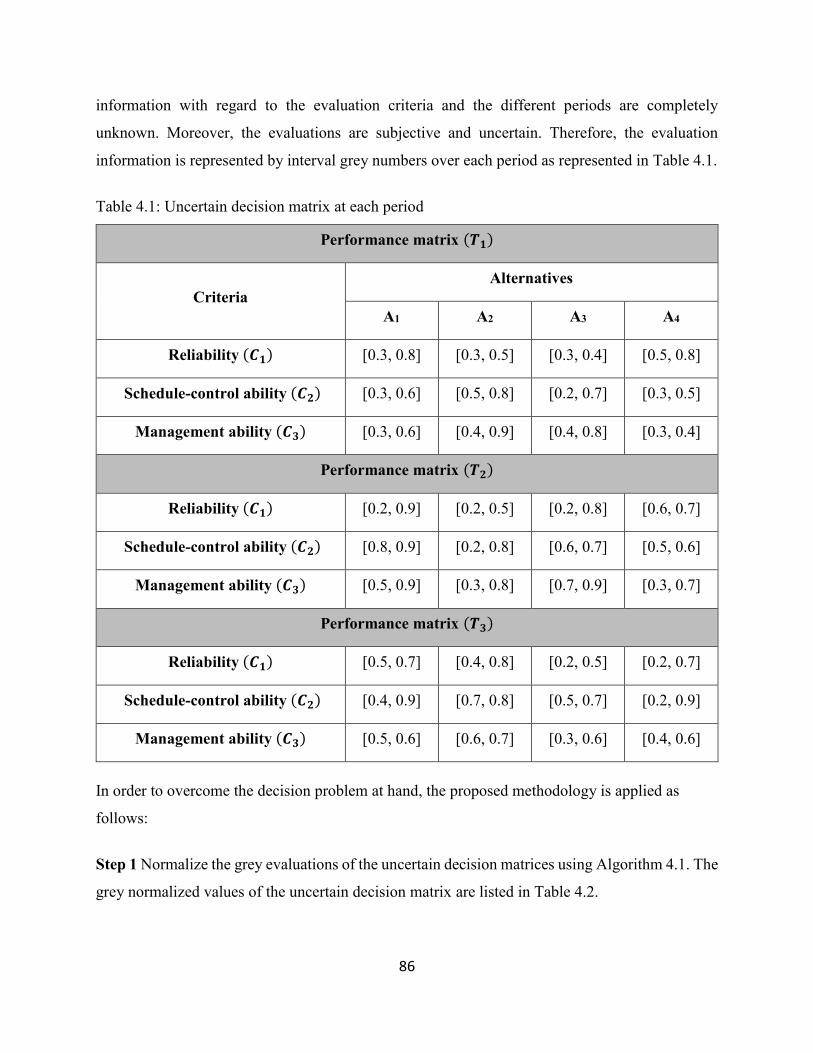
86
information with regard to the evaluation criteria and the different periods are completely
unknown. Moreover, the evaluations are subjective and uncertain. Therefore, the evaluation
information is represented by interval grey numbers over each period as represented in Table 4.1.
Table 4.1: Uncertain decision matrix at each period
Performance matrix (𝑻𝟏)
Criteria
Alternatives
A1 A2 A3 A4
Reliability (𝑪𝟏) [0.3, 0.8] [0.3, 0.5] [0.3, 0.4] [0.5, 0.8]
Schedule-control ability (𝑪𝟐) [0.3, 0.6] [0.5, 0.8] [0.2, 0.7] [0.3, 0.5]
Management ability (𝑪𝟑) [0.3, 0.6] [0.4, 0.9] [0.4, 0.8] [0.3, 0.4]
Performance matrix (𝑻𝟐)
Reliability (𝑪𝟏) [0.2, 0.9] [0.2, 0.5] [0.2, 0.8] [0.6, 0.7]
Schedule-control ability (𝑪𝟐) [0.8, 0.9] [0.2, 0.8] [0.6, 0.7] [0.5, 0.6]
Management ability (𝑪𝟑) [0.5, 0.9] [0.3, 0.8] [0.7, 0.9] [0.3, 0.7]
Performance matrix (𝑻𝟑)
Reliability (𝑪𝟏) [0.5, 0.7] [0.4, 0.8] [0.2, 0.5] [0.2, 0.7]
Schedule-control ability (𝑪𝟐) [0.4, 0.9] [0.7, 0.8] [0.5, 0.7] [0.2, 0.9]
Management ability (𝑪𝟑) [0.5, 0.6] [0.6, 0.7] [0.3, 0.6] [0.4, 0.6]
In order to overcome the decision problem at hand, the proposed methodology is applied as
follows:
Step 1 Normalize the grey evaluations of the uncertain decision matrices using Algorithm 4.1. The
grey normalized values of the uncertain decision matrix are listed in Table 4.2.
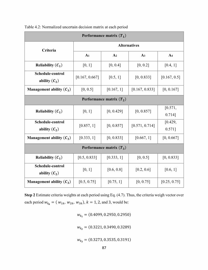
87
Table 4.2: Normalized uncertain decision matrix at each period
Performance matrix (𝑻𝟏)
Criteria
Alternatives
A1 A2 A3 A4
Reliability (𝑪𝟏) [0, 1] [0, 0.4] [0, 0.2] [0.4, 1]
Schedule-control
ability (𝑪𝟐) [0.167, 0.667] [0.5, 1] [0, 0.833] [0.167, 0.5]
Management ability (𝑪𝟑) [0, 0.5] [0.167, 1] [0.167, 0.833] [0, 0.167]
Performance matrix (𝑻𝟐)
Reliability (𝑪𝟏) [0, 1] [0, 0.429] [0, 0.857] [0.571,
0.714]
Schedule-control
ability (𝑪𝟐) [0.857, 1] [0, 0.857] [0.571, 0.714]
[0.429,
0.571]
Management ability (𝑪𝟑) [0.333, 1] [0, 0.833] [0.667, 1] [0, 0.667]
Performance matrix (𝑻𝟑)
Reliability (𝑪𝟏) [0.5, 0.833] [0.333, 1] [0, 0.5] [0, 0.833]
Schedule-control
ability (𝑪𝟐) [0, 1] [0.6, 0.8] [0.2, 0.6] [0.6, 1]
Management ability (𝑪𝟑) [0.5, 0.75] [0.75, 1] [0, 0.75] [0.25, 0.75]
Step 2 Estimate criteria weights at each period using Eq. (4.7). Thus, the criteria weigh vector over
each period 𝑤𝒕𝒌 = ( 𝑤1𝑘, 𝑤2𝑘, 𝑤3𝑘), 𝑘 = 1, 2, and 3, would be:
𝑤𝒕𝟏 = (0.4099, 0.2950, 0.2950)
𝑤𝒕𝟐 = (0.3221, 0.3490, 0.3289)
𝑤𝒕𝟑 = (0.3273, 0.3535, 0.3191)

88
Step 3 Estimate the weight of each period with respect to each criterion using Eq. (4.18). Thus,
the weight vector of each period with respect to each criterion 𝜃𝑗 = {𝜃𝑗 (𝑡1), 𝜃𝑗 (𝑡2), 𝜃𝑗 (𝑡3)}, 𝑗 =
1, 2, and 3, would be:
𝜃1 = (0.3869, 0.3041, 0.3090)
𝜃2 = (0.2958, 0.3499, 0.3544)
𝜃3 = (0.3129, 0.3487, 0.3384)
Step 4 Evaluate the preferences between the alternatives using Eq. (4.33). Take alternative 𝐴1 over
period 𝑇1 for example, Table 4.3 shows the preference degrees of 𝐴1 over other alternatives within
period 𝑇1.
Table 4.3: Preference matrix of A1 over T1
Multi-criteria preference matrix Alternatives
Base alternative Criteria A2 A3 A4
A1
Reliability (𝑪𝟏) 0.714 0.833 0.375
Schedule-control ability (𝑪𝟐) 0.167 0.500 0.600
Management ability (𝑪𝟑) 0.250 0.286 0.750
Step 5 Determine relative preferences by considering the calculated degrees of preferences
between the alternatives, the criteria weights, and the associated time period weight; using Eq.
(4.34). For illustration, Table 4.4 reflects the relative preference measures of alternative 𝐴1 over
other alternatives within period 𝑇1.
Step 6 Establish global preferences among alternatives using Eqs. (4.35), (4.36), and (4.37):
�̃� (𝐴1) = 0.1829, �̃� (𝐴2) = 0.0834, �̃� (𝐴3) = −0.2024, �̃� (𝐴4) = −0.0639
Step 7 Rank the alternatives and select the best one(s) in accordance with the net outranking flow
values:

89
𝐴1 ≻ 𝐴2 ≻ 𝐴4 ≻ 𝐴3
Thus, alternative 𝐴1 is the appropriate subcontractor for the uncertain DMCDM problem.
Table 4.4: Relative preference matrix of A1 over T1
Multi-criteria preference matrix Alternatives
Base alternative Criteria A2 A3 A4
A1
Reliability (𝑪𝟏) 0.113 0.132 0.059
Schedule-control ability (𝑪𝟐) 0.015 0.044 0.052
Management ability (𝑪𝟑) 0.023 0.026 0.069
4.5 Comparative analysis
By comparing the obtained ranking order for the adopted subcontractor selection case using
the proposed methodology in this manuscript with the original results of Peng and Wang (2014)
using dynamic interval-valued hesitant fuzzy aggregation operators, similar ranking order was
obtained.
Furthermore, Peng and Wang (2014) proposed another approach where dynamic hesitant fuzzy
aggregation operators were used to handle uncertain DMCDM problems. Likewise, the same
example was analyzed using hesitant fuzzy information instead of interval hesitant fuzzy
information. Once again, the proposed methodology in this manuscript provided the same ranking
order.
The advantages of the proposed methodology over the work of Peng and Wang (2014) can be
summarized as follows: (1) the original work presumed that decision makers are able to assign
criteria weights precisely, which is hardly the case in practical applications especially with
decision problems under uncertainty. In contrast, the proposed methodology is able to overcome a
more complicated DMCDM problems, in which the criteria weights are completely unknown using
the available information on alternatives evaluations; (2) the original work adapted the concept of
the BUM function for obtaining the weight vector of different periods, which does so
90
independently from the evaluation criteria. In contrast, the proposed methodology estimates the
weight vector of different time periods considering the changing in the influence of each evaluation
criterion over different periods. Thus, the dynamic aspects of different criteria are considered in
the proposed methodology, which have not been considered in BUM or other existing methods for
obtaining the weight vector of time periods.
4.6 Conclusion
Conventional MCDM approaches are not suitable to address the dynamics over time.
Therefore, different hybrid approaches have been developed to deal with DMCDM problems.
Different issues with the existing approaches have been identified in this research: (1) Criteria
weights: the overall evaluation of MCDM problems is based on alternatives evaluations and the
criteria weights, existing approaches in DMCDM problems assumes that information about criteria
weights is known, static over different periods, and/or can be assigned by decision makers.
However, there are cases where information on criteria weights is completely unknown due to
different reasons (e.g., time pressure, limited expertise, incomplete knowledge, and lack of
information), which would be an obstacle for the overall evaluations; (2) Weight vector
establishment of different time periods: within the context of DMCDM, the existing approaches
which estimate weight vector of different time periods does not consider the variabilities in the
influence of different criteria over different periods.
To overcome the shortcomings of the existing approaches, this manuscript is provided. It
investigates DMCDM problems with small amount of data and poor information, which cannot be
described by a probability distribution, where information on criteria weights and the influence of
different time periods are unknown. To this end, a new hybrid DMCDM methodology is proposed.
At first, consistency among evaluations over each period should be established. After that, the
unknown criteria weights should be estimated over each period; thus, an optimization model was
established based on the integration of grey system theory’s principles and the maximizing
deviation method. By solving the optimization model, a function to determine the optimal criteria
weights was obtained. Subsequently, the weight vector of different time periods with respect to
each evaluation criterion would be established using a new optimization model where the
evaluation space over a DMCDM problem would be maximized. Consequently, the DGMCDM

91
problem would be evaluated using a combination of the possibility degrees and PROMETHEE II.
Once the evaluation process is completed, the rank index for potential alternatives would be
provided based on the values of global preferences; in which the higher the value, the better is the
alternative.
To determine the feasibility and practicability of the proposed methodology, an existing case
in the literature was adopted; whereas to validate the methodology, a comparative analysis with
existing approaches was provided.
The advantages of this manuscript over other existing research works can be summarized in
the following points: (1) Estimate unknown criteria weights within the context of DMCDM
problems with small amount of data and poor information, which cannot be described by a
probability distribution, using the maximizing deviation method where the deviation degrees
functions are based on the principles of grey systems theory; (2) Establish the unknown weight
vector of different time periods by introducing a new optimization model, which considers the
changing in the influence of the different evaluation criteria over different periods; (3) Extend the
PROMETHE II approach to evaluate and rank potential alternatives within the context of
DMCDM problems using the optimized weights and the possibility degrees.
92
Chapter 5
Conclusions, Contributions and Future Research
5.1 Concluding remarks
MCDM is well recognized branch of operation research that intended to aid DMs in complex
decision problems, where different types of criteria of different nature should be considered. A
variety of MCDM approaches exist to address decision problems of different nature. However, the
various approaches of MCDA can be classified into three main categories: value measurement
models; goal, aspiration, or reference-level models; and outranking models.
The conventional approaches of MCDM have an implicit assumption, which presumes the
availability and accuracy of information. However, in many real life applications available
information is subject to uncertainty, imprecision, and subjectivity; which renders the conventional
approaches insufficient to handle the associated decision problem.
Although different hybrid methodologies have been introduced to handle the lack of accurate
information in a MCDM, there exist decision problems with small amount of data and poor
information in which the applicability of existing approaches would be influenced. Accordingly,
this manuscript-based thesis is intended to address decision problems that involve uncertain
evaluations due to lack of information. The significance of this thesis is highlighted in the
followings: (1) It focuses on MCDM problems under uncertain evaluations with small amount of
data and poor information. (2) It assesses different alternatives over complex interrelated decision
structure, which are subject to subjective and objective uncertain evaluations. (3) It provides a
systematic approach to carry out the overall evaluation for MCDM problems with small amount
of data and poor information, where information on criteria weight is unknown completely. (4) It
addresses DMCDM problems with small amount of data and poor information where information
on criteria weights and the weight vector of different time periods are unknown. (5) It considers
the fluctuations in the influence of different evaluation criteria on a decision problem over different
time periods. (6) It maximizes the evaluation space over MCDM and DMCDM with small amount
of data and poor information.

93
The conceptual and methodological contributions of this thesis to the current literature are
presented in the following subsections.
5.2 Conceptual contributions
This research proposed a new systematic methodology to address the limitation of
conventional MCDM approaches when uncertainty related aspects are present in a decision
problem. Different types of uncertainty related aspects are considered in the proposed approach:
(i) uncertainty associated with limited objective information, e.g., quantitative (interval scales),
and (ii) uncertainty associated with subjective expert knowledge (i.e., ambiguous concepts and
semantic meanings).
Although there exist different hybrid approaches to address different types of uncertainty, the
applicability of the existing approaches are limited when it comes to handle MCDM problems with
a relatively small amount of data and poor information, where evaluation criteria are of different
nature and interdependencies exist among them. This type of MCDM problem has been tackled in
the first manuscript of this thesis by considering interactions and interdependencies within and
between different evaluation clusters of a complex system, using linguistic expressions to
articulate DMs’ preferences, and employing range of values instead of exact values to map
linguistic expressions.
One of the major contributions of this research is to optimize the evaluation space over
uncertain MCDM problems, where the influence of each criterion over the decision problem is
unknown completely as a result of different reasons, such as time pressure, limited expertise,
incomplete knowledge and lack of information. The second manuscript of this thesis proposes a
new approach to tackle this type of MCDM problems. The concept behind the proposed approach
is to emphasize criteria that reflect larger deviations among alternatives. Thus, criteria which make
larger deviations should be assigned higher weights in comparison to criteria which make smaller
deviations.
Another contribution of this research is to handle MCDM problems within a dynamic context,
in which uncertain evaluations from different periods are provided, while information on the
influence of different criteria and the different periods over a decision problem are unknown

94
completely. Although there exist a number of approach to address dynamic MCDM problems, this
thesis presents in the third manuscript the first attempt that focuses on the variabilities in the
influence of the evaluation criteria throughout the different periods.
5.3 Methodological contributions
This manuscript-based thesis is intended to address a number of shortcomings in the existing
approaches associated with the modeling and analysis of MCDM with a relatively small amount
of data and poor information.
The first challenge was to optimize the evaluation space in decision problems that are subject
to subjective and objective uncertainty over different types of interrelated criteria (i.e., evaluation
criteria with different nature, different scales, and different values). To this end, the first
manuscript proposes a four-phased methodology, in which grey systems theory is integrated with
a distinctive combination of MCDM approaches (i.e., ANP and PROMETHEE II) as follows: the
grey systems theory is utilized to articulate the associated uncertainty with subjective and objective
evaluations; the principles of ANP is used to handle the complexity of the decision structure; the
PROMETHEE II approach is extended to evaluate and rank potential alternatives over interrelated
criteria under uncertain evaluations. The emergent strengths of the integrated approach should
improve the evaluation space in such a complex decision problem under uncertainty. To validate
the proposed methodology, a comparative analysis is put forward with the work of Kuo, Hsu, and
Chen (2015), which used fuzzy theory to address the uncertain related aspects. Although both
approaches reflect the same ranking order of available alternatives, yet the proposed methodology
is suitable to address decision problems with a relatively small amount of data and poor
information since it uses grey systems theory, which is preferred over fuzzy theory in such a
decision problem context where available information cannot be used to draw a robust membership
function that is required to carry out fuzzy theory’s calculations.
In the second manuscript, a more complicated scenario of MCDM problems within the context
of small amount of data and poor information was considered in which information on criteria
weights was completely unknown. The first phase was concerned with criteria weights estimation.
Accordingly, a new optimization model was introduced using the maximizing deviation method
95
and the principles of grey systems theory, where various scenarios of deviation were considered
to generalize the model. In the light of the proposed optimization model, a new function was
obtained to determine the optimal criteria weights in such MCDM problems. In the second phase,
potential alternatives were evaluated and ranked based on the integration of PROMETHEE II and
degrees of possibility, where the resultant criteria weights from the first phase were used as inputs
for the evaluation process. In order to validate the proposed methodology, a comparative analysis
with the work of Xu (2015) is carried out. The conclusion of the analysis indicates that three factors
influence alternatives ranking order, i.e., normalization approach, deviation function, and
alternative evaluation and ranking methodology. Moreover, a wider deviation area is covered
under the proposed methodology, which promotes the use of it over the work of Xu (2015).
In the third manuscript, the dynamic aspect of MCDM is investigated, in which evaluations
over different criteria change throughout the time while information on criteria weights and the
influence of different time periods is completely unknown. Although a number of approaches have
been introduced to address DMCDM, a number of shortcomings in the existing approaches are
identified in terms of criteria weights evaluations and the weight vector establishment of different
time periods. Consequently, a new hybrid DMCDM methodology is developed. The proposed
methodology targets three research problems: (1) establish priorities among evaluation criteria
over different time periods; (2) estimate weight vectors of different time periods considering the
variabilities in the influence of the evaluation criteria over the different periods to maximize the
evaluation space over a DMCDM; (3) evaluate and rank potential alternatives over DMCDM
problems with a relatively small amount of data and poor information. To validate the proposed
methodology, a comparative analysis with existing approaches (Peng & Wang, 2014) is
established. Although, the proposed methodology arrive to the same conclusion of Peng and Wang
(2014) with respect to alternatives ranking order, the proposed methodology surpass the work of
Peng and Wang (2014) in a number of issues: (1) providing a systematic approach to establish
criteria weights, where information on criteria weights is unknown; (2) considering the fluctuations
in the influence of different evaluation criteria on a decision problem over different time periods,
while estimating weight vectors of different time periods to maximize the evaluation space in a
dynamic decision problem.

96
5.4 Ideas for future research
The increased complexity of many decision problems makes it essential to look after
specialized knowledge, this impose the need of involving a number of DMs to build upon their
various knowledge and experience. In this thesis, it is assumed that consensus can be reached
among DMs or there is only one decision maker. However, conflicts in interests among decision
makers may raise; hence, the proposed methodologies can be enhanced by incorporating a conflict
resolution technique in future works. Moreover, the criticality of a DM can be considered in terms
of the level of related knowledge and expertise to the given decision problem, also the level of
authority among DMs. To this end, interactions among the involved DMs can be simulated to
provide valuable insights about the influence of a DM and the degree of involvement in a given
decision.
The learning curve within a dynamic decision environment can be considered as a factor in
order to improve perceptions of DMs, and thereby enhance their judgments.
Finally, real-world applications within the context of MCDM can be analyzed using the
proposed methodologies to refine and modify the methodologies. Also, the real data of these
applications can be simulated to demonstrate the feasibility of the proposed approaches; for
instance, uncertain evaluations and weights information can be generated from the corresponding
distributions, then the approximated values are used in the proposed functions. After a number of
iterations, criteria weights, alternatives ranking order and confidence factor can be obtained.
5.5 Related publications
During the course of work on this thesis, the following list of papers have been integrated into
the writing of it:
5.3.1 Journal papers
Maghrabie, H., Schiffauerova, A. & Beauregard, Y. “Grey-based Multi-Criteria Decision
Analysis Approach: Addressing Uncertainty at Complex Decision Problems”, Technological
Forecasting & Social Change. Submitted on October 2017.

97
Maghrabie, H., Beauregard, Y. & Schiffauerova, A., “Multi-Criteria Decision-Making Problems
with Unknown Weight Information under Uncertain Evaluations”, Computers & Industrial
Engineering. Submitted on November 2017.
Maghrabie, H., Beauregard, Y. & Schiffauerova, A., “A New Approach to Address Uncertain
Dynamic Multi-Criteria Decision Problems with Unknown Weight Information”, Expert Systems
with Applications. Submitted on February 2018.
5.3.2 Conference papers
Maghrabie, H., Schiffauerova, A., & Beauregard, Y. (2016). The use of Grey Systems Theory
in Complex Decision Problems under Uncertainty. Presented at MOSIM annual meeting 2016,
Montreal, QC, Canada.
Maghrabie, H., Schiffauerova, A., & Beauregard, Y. (2016). Grey based Multi Criteria
Decision Analysis to Address Multi Criteria Decision Problems under Uncertainty . Presented
at GDN annual meeting 2016, Bellingham, WA, United States.
Maghrabie, H., Schiffauerova, A., & Beauregard, Y. (2015). Improving the Front End
Innovation - Systems Engineering Approach. Presented at INFORMS annual meeting 2015,
Philadelphia, PA, United States.

98
References
Andreopoulou, Z., Koliouska, C., Galariotis, E., & Zopounidis, C. (2017). Renewable energy sources:
Using PROMETHEE II for ranking websites to support market opportunities. Technological
Forecasting and Social Change. https://doi.org/10.1016/J.TECHFORE.2017.06.007
Ang, J. L. F., Lee, W. K., Ooi, B. Y., & Ooi, T. W. M. (2017). An IPS Evaluation Framework for
Measuring the Effectiveness and Efficiency of Indoor Positioning Solutions. In K. Kim & N. Joukov
(Eds.), Information Science and Applications 2017: ICISA 2017 (pp. 688–697). Singapore: Springer
Singapore. https://doi.org/10.1007/978-981-10-4154-9_79
Antunes, C. H., & Henriques, C. O. (2016). Multi-Objective Optimization and Multi-Criteria Analysis
Models and Methods for Problems in the Energy Sector (pp. 1067–1165). Springer, New York, NY.
https://doi.org/10.1007/978-1-4939-3094-4_25
Awasthi, A., & Kannan, G. (2016). Green supplier development program selection using NGT and
VIKOR under fuzzy environment. Computers & Industrial Engineering, 91, 100–108.
https://doi.org/10.1016/J.CIE.2015.11.011
Bai, C., Sarkis, J., Wei, X., & Koh, L. (2012). Evaluating ecological sustainable performance measures
for supply chain management. Supply Chain Management: An International Journal, 17(1), 78–92.
https://doi.org/http://dx.doi.org/10.1108/13598541211212221
Baker, W. E., Grinstein, A., & Harmancioglu, N. (2016). Whose innovation performance benefits more
from external networks: entrepreneurial or conservative firms?. Journal of Product Innovation
Management, 33(1), 104–120. https://doi.org/10.1111/jpim.12263
Banaeian, N., Mobli, H., Fahimnia, B., & Nielsen, I. E. (2018). Green supplier selection using fuzzy
group decision making methods: A case study from the agri-food industry. Computers & Operations
Research, 89, 337–347. https://doi.org/10.1016/J.COR.2016.02.015
Belton, V., & Stewart, T. (2002). Multiple criteria decision analysis: an integrated approach. Springer
Science & Business Media.
Brans, J.-P., & De Smet, Y. (2016). PROMETHEE Methods. In Multiple Criteria Decision Analysis (pp.
187–219). Springer New York. https://doi.org/10.1007/978-1-4939-3094-4_6
Broekhuizen, H., Groothuis-Oudshoorn, C. G. M., Til, J. A., Hummel, J. M., & IJzerman, M. J. (2015). A
Review and Classification of Approaches for Dealing with Uncertainty in Multi-Criteria Decision
Analysis for Healthcare Decisions. PharmacoEconomics, 33(5), 445–455.
https://doi.org/10.1007/s40273-014-0251-x
Bronzini, R., & Piselli, P. (2016). The impact of R&D subsidies on firm innovation. Research Policy,
45(2), 442–457. https://doi.org/http://dx.doi.org/10.1016/j.respol.2015.10.008
Broumi, S., Ye, J., & Smarandache, F. (2015). An Extended TOPSIS Method for Multiple Attribute
Decision Making based on Interval Neutrosophic Uncertain Linguistic Variables. Neutrosophic Sets
& Systems, 8, 22–31.
Celik, E., Erdogan, M., & Gumus, A. T. (2016). An extended fuzzy TOPSIS–GRA method based on
different separation measures for green logistics service provider selection. International Journal of
Environmental Science and Technology, 13(5), 1377–1392. https://doi.org/10.1007/s13762-016-
0977-4

99
Chen, T.-Y. (2018). Remoteness index-based Pythagorean fuzzy VIKOR methods with a generalized
distance measure for multiple criteria decision analysis. Information Fusion, 41, 129–150.
https://doi.org/10.1016/J.INFFUS.2017.09.003
Chi, P., & Liu, P. (2013). An Extended TOPSIS Method for the Multiple Attribute Decision Making
Problems based on Interval Neutrosophic Set. Neutrosophic Sets and Systems, (1), 63–70.
Cohen, D., Lee, T., & Sklar, D. (2011). Precalculus. Brooks Cole.
Das, S., Dutta, B., & Guha, D. (2016). Weight computation of criteria in a decision-making problem by
knowledge measure with intuitionistic fuzzy set and interval-valued intuitionistic fuzzy set. Soft
Computing, 20(9), 3421–3442. https://doi.org/10.1007/s00500-015-1813-3
Dincer, H., Hacioglu, U., Tatoglu, E., & Delen, D. (2016). A fuzzy-hybrid analytic model to assess
investors’ perceptions for industry selection. Decision Support Systems, 86, 24–34.
https://doi.org/10.1016/j.dss.2016.03.005
Dodgson, J., Spackman, M., Pearman, A., & Phillips, L. (2009). Multi-criteria analysis: a manual.
Department for Communities and Local Government: London. https://doi.org/10.1002/mcda.399
Dokmanic, I., Parhizkar, R., Ranieri, J., & Vetterli, M. (2015). Euclidean Distance Matrices: Essential
theory, algorithms, and applications. IEEE Signal Processing Magazine, 32(6), 12–30.
https://doi.org/10.1109/MSP.2015.2398954
Dou, Y., Zhu, Q., & Sarkis, J. (2014). Evaluating green supplier development programs with a grey-
analytical network process-based methodology. European Journal of Operational Research, 233(2),
420–431. https://doi.org/10.1016/j.ejor.2013.03.004
Durbach, I. N., & Stewart, T. J. (2012). Modeling uncertainty in multi-criteria decision analysis.
European Journal of Operational Research, 223(1), 1–14.
https://doi.org/10.1016/j.ejor.2012.04.038
Eren, M., & Kaynak, S. (2017). An evaluation of EU member states according to human development and
global competitiveness dimensions using the multi-period grey relational analysis (MP-GRA)
technique. Grey Systems: Theory and Application, 7(1), 60–70. https://doi.org/10.1108/GS-08-2016-
0023
Ertay, T., Büyüközkan, G., Kahraman, C., & Ruan, D. (2005). Quality function deployment
implementation based on analytic network process with linguistic data : An application in
automotive industry. Journal of Intelligent & Fuzzy Systems, 16(3), 221–232.
Esangbedo, M. O., & Che, A. (2016). Grey Weighted Sum Model for Evaluating Business Environment
in West Africa. Mathematical Problems in Engineering, 2016, 1–14.
https://doi.org/10.1155/2016/3824350
Gao, J., & Liu, H. (2016). A New Prospect Projection Multi-Criteria Decision-Making Method for
Interval-Valued Intuitionistic Fuzzy Numbers. Information, 7(4), 64.
https://doi.org/10.3390/info7040064
Gebauer, H., Worch, H., & Truffer, B. (2012). Absorptive capacity , learning processes and combinative
capabilities as determinants of strategic innovation. European Management Journal, 30(1), 57–73.
https://doi.org/http://dx.doi.org/10.1016/j.emj.2011.10.004
Görener, A. (2012). Comparing AHP and ANP: An Application of Strategic Decisions Making in a
Manufacturing Company. International Journal of Business and Social Science, 3(11), 194–208.

100
Greco, S., Ehrgott, M., & Figueira, J. R. (Eds.). (2016). Multiple Criteria Decision Analysis. Springer-
Verlag New York.
Groothuis-Oudshoorn, C. G. M., Broekhuizen, H., & van Til, J. (2017). Dealing with Uncertainty in the
Analysis and Reporting of MCDA. In Multi-Criteria Decision Analysis to Support Healthcare
Decisions (pp. 67–85). Cham: Springer International Publishing. https://doi.org/10.1007/978-3-319-
47540-0_5
Gümüş, S., & Bali, O. . (2017). Dynamic Aggregation Operators Based on Intuitionistic Fuzzy Tools and
Einstein Operations. Fuzzy Information and Engineering, 9(1), 45–65.
https://doi.org/10.1016/j.fiae.2017.03.003
Hosseini, L., Tavakkoli-Moghaddam, R., Vahdani, B., Mousavi, S. M., & Kia, R. (2013). Using the
Analytical Network Process to Select the Best Strategy for Reducing Risks in a Supply Chain.
Journal of Engineering, 2013. https://doi.org/http://dx.doi.org/10.1155/2013/375628
Hsu, W. (2015). A Fuzzy Multiple-Criteria Decision-Making System for Analyzing Gaps of Service
Quality. International Journal of Fuzzy Systems, 17(2), 256–267. https://doi.org/10.1007/s40815-
015-0018-3
Ishizaka, A., & Labib, A. (2011). Review of the main developments in the analytic hierarchy process.
Expert Systems with Applications. https://doi.org/10.1016/j.eswa.2011.04.143
Jaini, N., & Utyuzhnikov, S. (2017). Trade-off ranking method for multi-criteria decision analysis.
Journal of Multi-Criteria Decision Analysis, 24(3–4), e1600. https://doi.org/10.1002/mcda.1600
Jianbo, X., Suihuai, Y., & Wen, F. (2016). Evaluation of Man-Machine System for Workover Rigs Based
on Grey Analytical Hierarchy Process. In 2016 Eighth International Conference on Measuring
Technology and Mechatronics Automation (ICMTMA) (pp. 278–281). IEEE.
https://doi.org/10.1109/ICMTMA.2016.75
Ju-long, D. (1982). Control problems of grey systems. Systems & Control Letters, 1(5), 288–294.
https://doi.org/https://doi.org/10.1016/S0167-6911(82)80025-X
K.Patil, S., & Kant, R. (2014). A fuzzy AHP-TOPSIS framework for ranking the solutions of Knowledge
Management adoption in Supply Chain to overcome its barriers. Expert Systems with Applications,
41(2), 679–693. https://doi.org/10.1016/J.ESWA.2013.07.093
Karsak, E. E., & Dursun, M. (2015). An integrated fuzzy MCDM approach for supplier evaluation and
selection. Computers & Industrial Engineering, 82, 82–93.
https://doi.org/10.1016/J.CIE.2015.01.019
Kilic, H. S., Zaim, S., & Delen, D. (2015). Selecting “The Best” ERP system for SMEs using a
combination of ANP and PROMETHEE methods. Expert Systems with Applications, 42(5), 2343–
2352. https://doi.org/10.1016/j.eswa.2014.10.034
Kuang, H., Kilgour, D. M., & Hipel, K. W. (2015). Grey-based PROMETHEE II with application to
evaluation of source water protection strategies. Information Sciences, 294, 376–389.
https://doi.org/H. Kuang, D.M. Kilgour, K.W. Hipel, Grey-based PROMETHEE II with application
to evaluation of source water protection strategies, Inf. Sci. (Ny). 294 (2015) 376–389.
doi:10.1016/j.ins.2014.09.035
Kuo, R. J., Hsu, C. W., & Chen, Y. L. (2015). Integration of fuzzy ANP and fuzzy TOPSIS for evaluating
carbon performance of suppliers. International Journal of Environmental Science and Technology,
12(12), 3863–3876. https://doi.org/10.1007/s13762-015-0819-9

101
Kurka, T., & Blackwood, D. (2013). Selection of MCA methods to support decision making for
renewable energy developments. Renewable and Sustainable Energy Reviews, 27, 225–233.
https://doi.org/http://dx.doi.org/10.1016/j.rser.2013.07.001
Li, C., & Yuan, J. (2017). A New Multi-attribute Decision-Making Method with Three-Parameter Interval
Grey Linguistic Variable. International Journal of Fuzzy Systems, 19(2), 292–300.
https://doi.org/10.1007/s40815-016-0241-6
Li, D.-C., Chang, C.-J., Chen, C.-C., & Chen, W.-C. (2012). Forecasting short-term electricity
consumption using the adaptive grey-based approach—An Asian case. Omega, 40(6), 767–773.
https://doi.org/10.1016/j.omega.2011.07.007
Li, G., Kou, G., & Peng, Y. (2015). Dynamic fuzzy multiple criteria decision making for performance
evaluation. Technological and Economic Development of Economy, 21(5), 705–719.
https://doi.org/10.3846/20294913.2015.1056280
Li, G., Yamaguchi, D., & Nagai, M. (2007). A grey-based decision-making approach to the supplier
selection problem. Mathematical and Computer Modelling, 46(3), 573–581.
https://doi.org/http://dx.doi.org/10.1016/j.mcm.2006.11.021
Li, N., & Huiru, Z. (2016). Performance evaluation of eco-industrial thermal power plants by using fuzzy
GRA-VIKOR and combination weighting techniques. Journal of Cleaner Production, 135, 169–
183. https://doi.org/10.1016/J.JCLEPRO.2016.06.113
Liang, W., Zhang, X., & Liu, M. (2015). The Maximizing Deviation Method Based on Interval-Valued
Pythagorean Fuzzy Weighted Aggregating Operator for Multiple Criteria Group Decision Analysis.
Discrete Dynamics in Nature and Society, 2015, 1–15. https://doi.org/10.1155/2015/746572
Lin, Y.-H., Lee, P.-C., & Ting, H.-I. (2008). Dynamic multi-attribute decision making model with grey
number evaluations. Expert Systems with Applications, 35(4), 1638–1644.
https://doi.org/10.1016/j.eswa.2007.08.064
Liu, S., Forrest, J. Y. L., & Yang, Y. (2015). Grey system: thinking, methods, and models with
applications. In M. Zhou, H.-X. Li, & M. Weijnen (Eds.), Contemporary Issues in Systems Science
and Engineering (pp. 153–224). Hoboken, NJ, USA: JohnWiley & Sons, Inc.
https://doi.org/10.1002/9781119036821.ch4
Liu, S., & Lin, Y. (2006). Grey information: Theory and practical applications. Springer-Verlag London.
https://doi.org/10.1007/1-84628-342-6
Liu, S., & Lin, Y. (2006). Grey Numbers and Their Operations. In Grey Information: Theory and
Practical Applications (pp. 23–43). Springer-Verlag London. https://doi.org/10.1007/1-84628-342-6
Lolli, F., Ishizaka, A., Gamberini, R., Rimini, B., Ferrari, A. M., Marinelli, S., & Savazza, R. (2016).
Waste treatment: an environmental, economic and social analysis with a new group fuzzy
PROMETHEE approach. Clean Technologies and Environmental Policy, 18(5), 1317–1332.
https://doi.org/10.1007/s10098-015-1087-6
Maity, S. R., & Chakraborty, S. (2015). Tool steel material selection using PROMETHEE II method. The
International Journal of Advanced Manufacturing Technology, 78(9), 1537–1547.
https://doi.org/10.1007/s00170-014-6760-0
Małachowski, B. (2016). Multiple Criteria Decision Support System for Tender Consortium Building
Within the Cluster Organization. In New Frontiers in Information and Production Systems
Modelling and Analysis (pp. 105–117). Springer International Publishing.

102
https://doi.org/10.1007/978-3-319-23338-3_5
Malczewski, J., & Rinner, C. (2015). Multicriteria Decision Analysis in Geographic Information Science.
New York, NY, USA: Springer-Verlag Berlin Heidelberg. https://doi.org/10.1007/978-3-540-
74757-4
Mardani, A., Jusoh, A., MD Nor, K., Khalifah, Z., Zakwan, N., & Valipour, A. (2015). Multiple criteria
decision-making techniques and their applications – a review of the literature from 2000 to 2014.
Economic Research-Ekonomska Istraživanja, 28(1), 516–571.
https://doi.org/10.1080/1331677X.2015.1075139
Martín-de Castro, G. M. (2015). Knowledge management and innovation in knowledge-based and high-
tech industrial markets: The role of openness and absorptive capacity. Industrial Marketing
Management, 47, 143–146. https://doi.org/http://dx.doi.org/10.1016/j.indmarman.2015.02.032
Mazarr, M. J. (2016). Defining Risk. In Rethinking Risk in National Security: Lessons of the Financial
Crisis for Risk Management (pp. 19–34). New York: Palgrave Macmillan US.
https://doi.org/10.1007/978-1-349-91843-0_2
Mehrbakhsh, N., Ahmadi, H., Ahani, A., Ravangard, R., & Ibrahim, O. bin. (2016). Determining the
importance of Hospital Information System adoption factors using Fuzzy Analytic Network Process
(ANP). Technological Forecasting and Social Change, 111, 244–264.
https://doi.org/10.1016/J.TECHFORE.2016.07.008
Memon, M. S., Lee, Y. H., & Mari, S. I. (2015). A Combined Grey System Theory and Uncertainty
Theory-Based Approach for Supplier Selection in Supply Chain Management. In Toward
Sustainable Operations of Supply Chain and Logistics Systems (pp. 461–473). Springer International
Publishing. https://doi.org/10.1007/978-3-319-19006-8
Mendi, P., & Costamagna, R. (2017). Managing innovation under competitive pressure from informal
producers. Technological Forecasting & Social Change, 114, 192–202.
https://doi.org/http://dx.doi.org/10.1016/j.techfore.2016.08.013
Merigó, J. M., Palacios-Marqués, D., & Zeng, S. (2016). Subjective and objective information in
linguistic multi-criteria group decision making. European Journal of Operational Research, 248(2),
522–531. https://doi.org/10.1016/j.ejor.2015.06.063
Moos, B., Beimborn, D., Wagner, H. T., & Weitzel, T. (2013). The role of knowledge management
systems for innovation: An absorptive capacity perspective. International Journal of Innovation
Management, 17(5). https://doi.org/http://dx.doi.org/10.1142/S1363919613500199
Moretti, S., Öztürk, M., & Tsoukiàs, A. (2016). Preference Modelling. In S. Greco, M. Ehrgott, & J. R.
Figueira (Eds.), Multiple Criteria Decision Analysis: State of the Art Surveys (pp. 43–95). New
York, NY: Springer New York. https://doi.org/10.1007/978-1-4939-3094-4_3
Mu, E., & Pereyra-Rojas, M. (2017). Understanding the Analytic Hierarchy Process. In Practical
Decision Making (pp. 7–22). Springer, Cham. https://doi.org/10.1007/978-3-319-33861-3_2
Nguyen, H.-T., Dawal, S. Z. M., Nukman, Y., & Aoyama, H. (2014). A hybrid approach for fuzzy multi-
attribute decision making in machine tool selection with consideration of the interactions of
attributes. Expert Systems with Applications, 41(6), 3078–3090.
https://doi.org/10.1016/j.eswa.2013.10.039
Onetti, A., Zucchella, A., Jones, M. V., & McDougall-Covin, P. P. (2012). Internationalization,
innovation and entrepreneurship: business models for new technology-based firms. Journal of

103
Management & Governance, 16(3), 337–368. https://doi.org/10.1007/s10997-010-9154-1
Park, J. H., Cho, H. J., & Kwun, Y. C. (2013). Extension of the VIKOR method to dynamic intuitionistic
fuzzy multiple attribute decision making. Computers & Mathematics with Applications, 65(4), 731–
744. https://doi.org/10.1016/J.CAMWA.2012.12.008
Peng, D.-H., & Wang, H. (2014). Dynamic hesitant fuzzy aggregation operators in multi-period decision
making. Kybernetes, 43(5), 715–736. https://doi.org/10.1108/K-11-2013-0236
Pruyt, E. (2007). Dealing with Uncertainties? Combining System Dynamics with Multiple Criteria
Decision Analysis or with Exploratory Modelling. In Proceedings of the 25th International
Conference of the System Dynamics Society. Boston, USA.
Reid, S. E., & Brentani, U. De. (2015). Building a measurement model for market visioning competence
and its proposed antecedents: organizational encouragement of divergent thinking, divergent
thinking attitudes, and ideational behavior. Journal of Product Innovation Management, 32(2), 243–
262. https://doi.org/10.1111/jpim.12232
Roy, B. (2016). Paradigms and Challenges. In S. Greco, M. Ehrgott, & J. R. Figueira (Eds.), Multiple
Criteria Decision Analysis: State of the Art Surveys (pp. 19–39). Springer New York.
Ruiz-Padillo, A., Ruiz, D. P., Torija, A. J., & Ramos-Ridao, Á. (2016). Selection of suitable alternatives
to reduce the environmental impact of road traffic noise using a fuzzy multi-criteria decision model.
Environmental Impact Assessment Review, 61, 8–18. https://doi.org/10.1016/j.eiar.2016.06.003
Saaty, R. (2013). validation of the effectiveness of inner dependence in an ANP model. In The 12th
International Symposium on the Analytic Hierarchy Process.
Saaty, T. L. (1996). The Analytic Network Process: Decision Making with Dependence and Feedback.
Pittsburgh, PA: RWS Publications.
Saeidi, S. P., Sofian, S., Saeidi, P., Saeidi, S. P. S., & Saaeidi, S. A. (2015). How does corporate social
responsibility contribute to firm financial performance? The mediating role of competitive
advantage, reputation, and customer satisfaction. Journal of Business Research, 68(2), 341–350.
https://doi.org/http://dx.doi.org/10.1016/j.jbusres.2014.06.024
Şahin, R., & Liu, P. (2016). Maximizing deviation method for neutrosophic multiple attribute decision
making with incomplete weight information. Neural Computing and Applications, 27(7), 2017–
2029. https://doi.org/10.1007/s00521-015-1995-8
Sakthivel, G., Ilangkumaran, M., Nagarajan, G., Priyadharshini, V., Kumar, S. D., Kumar, S. S., …
Selvan, G. T. (2014). Multi-criteria decision modelling approach for biodiesel blend selection based
on GRA – TOPSIS analysis. International Journal of Ambient Energy, 35(3).
https://doi.org/10.1080/01430750.2013.789984
Schweizer, L. (2015). Integrating Multiple Case Studies with a Merger and Acquisition Example. In The
Palgrave Handbook of Research Design in Business and Management (pp. 319–339). New York:
Palgrave Macmillan US. https://doi.org/10.1057/9781137484956
Segura, M., & Maroto, C. (2017). A multiple criteria supplier segmentation using outranking and value
function methods. Expert Systems with Applications, 69, 87–100.
https://doi.org/10.1016/j.eswa.2016.10.031
Sen, D. K., Datta, S., Patel, S. K., & Mahapatra, S. S. (2015). Multi-criteria decision making towards
selection of industrial robot: Exploration of PROMETHEE II method. Benchmarking: An
International Journal, 22(3), 465–487. https://doi.org/http://dx.doi.org/10.1108/BIJ-05-2014-0046

104
Şengül, Ü., Eren, M., Shiraz, S. E., Gezderd, V., & Şengül, A. B. (2015). Fuzzy TOPSIS method for
ranking renewable energy supply systems in Turkey. Renewable Energy, 75, 617–625.
https://doi.org/10.1016/J.RENENE.2014.10.045
Shi, Y., Liu, H., & Sun, J. (2013). The cloud model based on grey system theory and application on
effectiveness evaluation. In D.-S. Huang, V. Bevilacqua, J. C. Figueroa, & P. Premaratne (Eds.),
Intelligent Computing Theories: 9th International Conference, ICIC 2013, Nanning, China, July 28-
31, 2013. Proceedings (pp. 31–38). Berlin, Heidelberg: Springer Berlin Heidelberg.
https://doi.org/10.1007/978-3-642-39479-9_4
Thakur, V., & Ramesh, A. (2017). Healthcare waste disposal strategy selection using grey-AHP approach.
Benchmarking: An International Journal, 24(3), 735–749. https://doi.org/10.1108/BIJ-09-2016-
0138
Torra, V. (2010). Hesitant fuzzy sets. International Journal of Intelligent Systems, 25(6).
https://doi.org/10.1002/int.20418
Tuzkaya, U. R., & Yolver, E. (2015). R&D project selection by integrated grey analytic network process
and grey relational analysis: an implementation for home appliances company. Journal of
Aeronautics and Space Technologies, 8(2), 35–41.
Tzokas, N., Ah, Y., Akbar, H., & Al-dajani, H. (2015). Absorptive capacity and performance: The role of
customer relationship and technological capabilities in high-tech SMEs. Industrial Marketing
Management, 47, 134–142. https://doi.org/http://dx.doi.org/10.1016/j.indmarman.2015.02.033
Velasquez, M., & Hester, P. T. (2013). An Analysis of Multi-Criteria Decision Making Methods, 10(2),
56–66.
Wang, P., Li, Y., Wang, Y.-H., & Zhu, Z.-Q. (2015). A New Method Based on TOPSIS and Response
Surface Method for MCDM Problems with Interval Numbers. Mathematical Problems in
Engineering, 2015, 1–11. https://doi.org/10.1155/2015/938535
Wang, Y. M. (1998). Using the method of maximizing deviations to make decision for multi-indices.
System Engineering and Electronics, 7(24-26), 31.
Wątróbski, J., & Jankowski, J. (2016). Guideline for MCDA Method Selection in Production
Management Area. In New Frontiers in Information and Production Systems Modelling and
Analysis (pp. 119–138). Springer International Publishing.
Wei, G.-W. (2008). Maximizing deviation method for multiple attribute decision making in intuitionistic
fuzzy setting. Knowledge-Based Systems, 21(8), 833–836.
https://doi.org/10.1016/J.KNOSYS.2008.03.038
Wei, G. (2011). Grey relational analysis model for dynamic hybrid multiple attribute decision making.
Knowledge-Based Systems, 24(5), 672–679. https://doi.org/10.1016/j.knosys.2011.02.007
Wei, G., & Lin, R. (2008). Dynamic Uncertain Linguistic Weighted Geometric Mean Operator. In 2008
Fifth International Conference on Fuzzy Systems and Knowledge Discovery (pp. 254–258). IEEE.
https://doi.org/10.1109/FSKD.2008.579
Xia, M., & Xu, Z. (2011). Hesitant fuzzy information aggregation in decision making. International
Journal of Approximate Reasoning, 52(3), 395–407. https://doi.org/10.1016/J.IJAR.2010.09.002
Xu, Z. (2015). Interval MADM with Unknown Weight Information. In Uncertain Multi-Attribute
Decision Making (pp. 177–205). Berlin, Heidelberg: Springer Berlin Heidelberg.
https://doi.org/10.1007/978-3-662-45640-8_5

105
Xu, Z., & Cai, X. (2012). Intuitionistic Fuzzy Information Aggregation. Berlin, Heidelberg: Springer
Berlin Heidelberg. https://doi.org/10.1007/978-3-642-29584-3
Xu, Z. S., & Da, Q. L. (2002). The uncertain OWA operator. International Journal of Intelligent Systems,
17(6), 569–575. https://doi.org/10.1002/int.10038
Xu, Z., & Zhang, X. (2013). Hesitant fuzzy multi-attribute decision making based on TOPSIS with
incomplete weight information. Knowledge-Based Systems, 52, 53–64.
https://doi.org/10.1016/J.KNOSYS.2013.05.011
Yager, R. R. (1998). Quantifier guided aggregation using OWA operators. International Journal of
Intelligent Systems, 11(1), 49–73. https://doi.org/10.1002/(SICI)1098-111X(199601)11:1<49::AID-
INT3>3.0.CO;2-Z
Yager, R. R. (2004). OWA Aggregation Over a Continuous Interval Argument With Applications to
Decision Making. IEEE Transactions on Systems, Man and Cybernetics, Part B (Cybernetics),
34(5), 1952–1963. https://doi.org/10.1109/TSMCB.2004.831154
Zadeh, L. A. (1965). Fuzzy sets. Information and Control, 8(3), 338–353. https://doi.org/10.1016/S0019-
9958(65)90241-X
Zaim, S., Sevkli, M., Camgöz-akdag, H., Demirel, O. F., Yayla, A. Y., & Delen, D. (2014). Expert
Systems with Applications Use of ANP weighted crisp and fuzzy QFD for product development.
Expert Systems with Applications, 41(9), 4464–4474.
https://doi.org/http://dx.doi.org/10.1016/j.eswa.2014.01.008
Zhang, S., & Liu, S. (2011). Expert Systems with Applications A GRA-based intuitionistic fuzzy multi-
criteria group decision making method. Expert Systems With Applications, 38(9), 11401–11405.
https://doi.org/10.1016/j.eswa.2011.03.012
Zhang, S., Liu, S., & Zhai, R. (2011). An extended GRA method for MCDM with interval-valued
triangular fuzzy assessments and unknown weights. Computers & Industrial Engineering, 61(4),
1336–1341. https://doi.org/10.1016/J.CIE.2011.08.008
Zhang, W., Zhang, X., Fu, X., & Liu, Y. (2009). A grey analytic network process (ANP) model to
identify storm tide risk. In IEEE International Conference on Grey Systems and Intelligent Services
(pp. 582–587). IEEE. https://doi.org/10.1109/GSIS.2009.5408247
Zhang, X., & Liu, P. (2010). Method for Multiple Attribute Decision-making under Risk with Interval
Numbers. International Journal of Fuzzy Systems, 12(3).
Zhou, H., Wang, J., & Zhang, H. (2017). Stochastic multicriteria decision-making approach based on
SMAA-ELECTRE with extended gray numbers. International Transactions in Operational
Research. https://doi.org/10.1111/itor.12380