Supplementary materials for this article are available online. Please click the JASA link at http://pubs.amstat.org.

Multi-Domain Sampling With Applications toStructural Inference of Bayesian Networks

Qing ZHOU

When a posterior distribution has multiple modes, unconditional expectations, such as the posterior mean, may not offer informative sum-maries of the distribution. Motivated by this problem, we propose to decompose the sample space of a multimodal distribution into domainsof attraction of local modes. Domain-based representations are defined to summarize the probability masses of and conditional expecta-tions on domains of attraction, which are much more informative than the mean and other unconditional expectations. A computationalmethod, the multi-domain sampler, is developed to construct domain-based representations for an arbitrary multimodal distribution. Themulti-domain sampler is applied to structural learning of protein-signaling networks from high-throughput single-cell data, where a signal-ing network is modeled as a causal Bayesian network. Not only does our method provide a detailed landscape of the posterior distributionbut also improves the accuracy and the predictive power of estimated networks. This article has supplementary material online.

KEY WORDS: Domain-based representation; Monte Carlo; Multimodal distribution; Network structure; Protein-signaling network;Wang–Landau algorithm.

1. INTRODUCTION

In Bayesian inference the information on an unknown pa-rameter θ given an observed dataset yobs is contained in theposterior distribution p(θ | yobs). When a posterior distributiondoes not belong to a well-characterized family of distributions,Markov chain Monte Carlo (MCMC) is a standard computa-tional approach to Bayesian inference via sampling from theposterior distribution. Typical examples of MCMC include theMetropolis–Hastings (MH) algorithm (Metropolis et al. 1953;Hastings 1970) and the Gibbs sampler (Geman and Geman1984; Tanner and Wong 1987; Gelfand and Smith 1990). Thor-ough reviews of recent developments on Monte Carlo methodsand their applications in Bayesian computation can be found inthe work of Chen, Shao, and Ibrahim (2001) and Liu (2008).The posterior mean E(θ | yobs) and other expectations are usu-ally approximated from a Monte Carlo sample to summarizethe posterior distribution. However, these unconditional expec-tations may not offer good summaries of the information forBayesian inference when a posterior distribution has multiplelocal modes. One can easily construct a multimodal posteriordistribution of which the mean is located in a low-density re-gion and thus using it as an estimator for θ lacks a conventionalinterpretation. To extract more information contained in a mul-timodal posterior distribution, it is desired to identify all majormodes and calculate various statistics in appropriate neighbor-hoods of these modes.

To achieve these tasks, we propose to partition the samplespace of θ into a collection of domains such that the poste-rior distribution restricted to each domain is unimodal. Themost parsimonious partition that minimizes the number of do-mains is to use the domains of attraction (to be defined rig-orously later) of the local modes. Take the trimodal distribu-tion p(θ) in Figure 1 as an illustration. The space is parti-tioned into three domains, denoted by �1,�2, and �3: Eachdomain contains exactly one local mode; if we move any θ ∈ �k

Qing Zhou is Assistant Professor, Department of Statistics, University ofCalifornia, Los Angeles, CA 90095 (E-mail: zhou@stat.ucla.edu). This workwas supported in part by NSF grant DMS-0805491 and NSF CAREER AwardDMS-1055286. The author thanks the editor, the associate editor, and the tworeferees for helpful comments and suggestions which significantly improvedthe manuscript.

(k = 1,2,3) along the trajectory that always follows the gradi-ent direction of p(θ), it will eventually reach the mode in thedomain �k. We may then calculate various conditional expec-tations on these domains, E[h(θ) | θ ∈ �k] (k = 1,2,3), for dif-ferent functions h. Together with the probability masses of thedomains, P(θ ∈ �k), they provide more informative summariesof the distribution p(θ) than unconditional expectations. Sucha summary is called a domain-based representation (DR) forp(θ).

Although desired, construction of DRs for an arbitrary dis-tribution is very challenging in practice. Sufficient Monte Carlosamples from domains of all local modes are necessary for es-timating DRs, but efficient sampling from a multimodal distri-bution has always been a hard problem. In this article, we de-velop a computational method that is able to construct domain-based representations for an arbitrary multimodal distribution.We partition the sample space into domains of attraction andutilize an iterative weighting scheme aiming at sampling fromeach domain with an equal frequency. The weighting schemewas proposed by Wang and Landau (2001), and further devel-oped and generalized by Liang (2005), Liang, Liu, and Carroll(2007), and Atchadé and Liu (2010), among others. However,a direct application of these existing methods cannot provideaccurate estimation of DRs, due to at least two reasons. First,sample space partition used in these methods is usually pre-determined according to a set of selected density levels. Butpartitioning the space into domains of attraction, as employedin our method, cannot be completed beforehand because it isa nontrivial job to detect all local modes and their domains inreal applications. Second, the above methods mostly rely onsimple local moves and lack a coherent global move to jumpbetween different local modes. To obtain accurate estimationof DRs, we propose a dynamic scheme to partition the samplespace into domains of attraction and devise a global move thatutilizes estimated DRs along sampling iterations to enable fasttransitions between multiple domains. Since the main feature of

© 2011 American Statistical AssociationJournal of the American Statistical Association

December 2011, Vol. 106, No. 496, Applications and Case StudiesDOI: 10.1198/jasa.2011.ap10346

1317

1318 Journal of the American Statistical Association, December 2011

Figure 1. Contour plot of a two-dimensional density with threemodes labeled A, B, and C. The numbers report log densities of con-tours and the dashed curves mark the boundaries between domains ofattraction.

our method is to sample from multiple domains and constructDRs, we call it the multi-domain (MD) sampler.

The MD sampler can be applied to a wide range of Bayesianinference problems and it is particularly powerful in tacklingproblems with complicated posterior distributions. Althoughthere are many such applications in different fields, this arti-cle mainly concerns structural learning of causal Bayesian net-works from experimental data. Learning network structure viaMonte Carlo sampling is very challenging as the multimodalityof the posterior distribution is extremely severe (Friedman andKoller 2003; Ellis and Wong 2008; Liang and Zhang 2009). Inthis problem, a domain of attraction is defined by a set of net-work structures, each represented by a directed acyclic graph(DAG). In a sense, the goal of the MD sampler is to constructa detailed landscape of the posterior distribution, which canprovide new insights into the structural learning problem. Ap-plication of our method to a scientific problem is illustratedby a study on constructing protein-signaling networks fromsingle-cell experimental data. A living cell is highly respon-sive to its environment due to the existence of widespread anddiverse signal transduction pathways. These pathways consti-tute a complex signaling network as cross-talks usually existbetween them. Knowledge of the structure of this network iscritical to the understanding of various cellular behaviors andhuman diseases. Recent advances in biotechnology allow thebiologist to measure the states of a collection of molecules ona cell-by-cell basis. Such large-scale data contain rich informa-tion for statistical inference of signaling networks, but powerfulcomputational methods are needed given the complexity in thelikelihood function and the posterior distribution. With the MDsampler, not only can we build a signaling network from theposterior mean graph, but also we may discover new pathwayconnections revealed by different domains of the posterior dis-tribution, which are not accessible by other approaches.

The remaining part of this article is organized as follows.Section 2 defines the domain of attraction and domain-basedrepresentation. In Section 3 we develop the MD sampler andits estimation of DRs, with convergence and ergodicity of thesampler established in the Appendix. The method is tested in

Section 4 on an example in Euclidean space and implementedin Section 5 for Bayesian inference of network structure with asimulation study. Section 6 is the main application to the con-struction of signaling networks in human T cells. The articleconcludes with a discussion on related and future works.

2. DOMAIN–BASED REPRESENTATION

Let p(x), x ∈ X ⊆ Rm, be the density of the target distribu-

tion. Suppose that p(x) is differentiable and denote by ∇p(x)

the gradient of p at x. Define a differential equation

dx(t)

dt= ∇p(x(t)) (1)

and write a solution path of this equation as x(t), t ∈ [0,∞),where x(0) is a chosen initial point. Under some mild regular-ity conditions, x(∞) converges to a local mode of p(x), whichis the basic intuition behind the gradient ascent algorithm tomaximize p(x). Denote by {ν1, . . . ,νK} all the local modes, in-cluding the global mode, of p(x). For x ∈ X , let x(0) = x anddefine the domain partition index by

I(x) ={

k, if x(∞) = νk, for k = 1, . . . ,K0, otherwise.

(2)

It maps x to the index of the local mode to which the solutionpath starting at x converges.

Definition 1. The domain of attraction of νk is Dk = {x ∈X : I(x) = k} for k = 1, . . . ,K. For simplicity we may call Dk

an attraction domain or a domain of p.

If the stationary points of p(x) have zero probability mass,then {Dk : k = 1, . . . ,K} form a partition of the sample space

X except for a set of zero probability mass. This is the defaultsetting for this article.

Let h(x) be a p-integrable function of x. Write the probabilitymass of Dk and the conditional expectation of h(X) given X ∈Dk as

λk = P(X ∈ Dk) =∫

Dk

p(x)dx, (3)

μh,k = E[h(X) | X ∈ Dk] = 1

λk

∫Dk

h(x)p(x)dx, (4)

respectively, for k = 1, . . . ,K.

Definition 2. The domain-based representation of h withrespect to the distribution p is a 2 × K array, DRp(h) ={(μh,k, λk) : k = 1, . . . ,K}.

The DR is equivalent to the probability mass function ofE[h(X) | I(X)] that assigns probability λk to μh,k for k =1, . . . ,K. It provides the expectation E[h(X)] = ∑

k λkμh,k

and the decomposed contributions from the attraction do-mains of p(x). Such a representation gives an informative low-dimensional summary of a multimodal distribution. For a com-plex distribution with many local modes, however, we cannotafford to estimate (μh,k, λk) for every domain when K is toolarge and are less interested in domains of negligible proba-bility masses (λk very close to zero). Due to these reasons wedefine domain-based representations with respect to a set oflocal modes {νk : k = 1, . . . ,M}. Index all the local modes as

Zhou: Multi-Domain Sampler 1319

ν1, . . . ,νM, . . . ,νK (M ≤ K). Define the domain partition in-dex with respect to {νk}M

k=1 by IM(x) = I(x) if 1 ≤ I(x) ≤ Mand IM(x) = 0 otherwise. Then the sample space X can bepartitioned into Dk = {x ∈ X : IM(x) = k} for k = 0, . . . ,M,where Dk is the domain of νk (k ≥ 1) and D0 = X − ⋃M

k=1 Dk.The DR of h with respect to {νk}M

k=1 is defined by the array{(μh,k, λk) : k = 0, . . . ,M}, where λ0 and μh,0 are defined forD0 similarly as in Equations (3) and (4), respectively. Notethat one can still obtain E[h(X)] = ∑M

k=0 λkμh,k after mergingDM+1, . . . ,DK into D0.

There is a geometric interpretation for the attraction domainsof a posterior distribution. Suppose that Y = (Y1, . . . ,Yn) is asample from an unknown distribution ψ(y). We assume a para-metric family fθ = f (· | θ), θ ∈ �, as the model for Y and put aprior π(θ) on the unknown parameter θ . The posterior distribu-tion of θ is given by

p(θ | Y) ∝ π(θ)

n∏i=1

f (Yi | θ) ≈ enE[log f (Y1|θ)]

when the sample size n is large, where E[log f (Y1 | θ)] =∫log[f (y | θ)]ψ(y)dy. Denote the Kullback–Leibler (KL) di-

vergence between ψ and fθ by

dKL(ψ‖fθ ) =∫

log

[ψ(y)

f (y | θ)

]ψ(y)dy.

Then, p(θ | Y) ∝ exp[−ndKL(ψ‖fθ )] when n is large. In thespace of density functions, we can regard dKL(ψ‖fθ ) as the “dis-tance” to the point ψ from a point in the manifold M = {fθ : θ ∈�}. Note that ψ is not necessarily in M if our model assump-tion on Y is incorrect. Then p(θ | Y) may be interpreted as aBoltzmann distribution on the manifold M under a potentialfield ndKL(ψ‖fθ ). This potential pushes every fθ , indexed by θ ,toward ψ , and the collection of θ which will be driven to anidentical stationary point in M forms an attraction domain ofp(θ | Y).

3. THE MULTI–DOMAIN SAMPLER

To develop an algorithm that is able to construct domain-based representations with respect to the target distribution p,it is necessary to identify the attraction domain of any x ∈ X .When p(x) is differentiable, this can be achieved by applicationof the gradient ascent (GA) algorithm that finds local modes ofp(x), or log p(x) for computational convenience. Generalizationto the space of network structures will be discussed later.

A naive two-step approach to the construction of DRs is quiteobvious. We may first apply a Monte Carlo algorithm to simu-late a sample {Xt}n

t=1 from p(x) or from a diffuse version ofp(x), for example, [p(x)]1/τ for τ > 1 as used in parallel tem-pering (Geyer 1991). Then, for every t we determine I(Xt) bya GA search initiated at Xt to find to which domain it belongs.This approach partitions the sample into attraction domains sothat we can estimate the probability masses and conditional ex-pectations for all identified domains. Although simple to im-plement, this two-step approach has a few drawbacks in termsof efficiency. Without a careful and specific design the MonteCarlo algorithm, even targeting at a diffuse version of p(x), maynot generate enough samples from all major domains or maycompletely miss some modes. As a result, estimation on some

attraction domains may be inaccurate or unavailable. In addi-tion, this approach does not utilize the information on the tar-get distribution provided by the constructed DRs. To overcomethese drawbacks, we develop the MD sampler that may achievesimultaneously an efficient simulation from a multimodal dis-tribution and an accurate construction of domain-based repre-sentations, with comparable computational complexity as thenaive two-step approach.

3.1 The Main Algorithm

We wish to sample sufficiently from the majority of attrac-tion domains. However, the density at the boundary betweentwo neighboring domains is often exponentially low (e.g., Fig-ure 1), which makes it difficult for an MH algorithm or a Gibbssampler to jump across multiple domains. Thus, we need to al-low the sampler to generate enough samples from such low-density regions that connect different domains. These consider-ations motivate the following double-partitioning design in theMD sampler.

Suppose that we are given a set of local modes of p(x),{ν1, . . . ,νM}, which may include the global mode. Given ∞ =H0 > H1 > · · · > HL = −∞, define the density partition indexJ(x) = j if log p(x) ∈ [Hj,Hj−1) for j = 1, . . . ,L. We partitionthe space X into (M + 1) × L subregions,

Dkj = {x ∈ X : IM(x) = k, J(x) = j},k = 0, . . . ,M, j = 1, . . . ,L, (5)

where IM(x) is the domain partition index with respect to{νk}M

k=1. Then, the attraction domain of the local mode νk isDk = ⋃

j Dkj (1 ≤ k ≤ M). Note that some Dkj may be empty;if log p(νk) < Hi, then all Dkj for j ≤ i are empty. In what fol-lows, we only consider nonempty subregions. For a given ma-trix W = (wkj)(M+1)×L, define a working density

p(x;W) ∝M∑

k=0

L∑j=1

p(x)1(x ∈ Dkj)

exp(wkj), (6)

where 1(·) is an indicator function. Let W∗ = (w∗kj) such that

exp(w∗kj) = ∫

Dkjp(x)dx. Then, the probability masses of Dkj are

identical under p(x;W∗). Sampling from p(x;W∗) has two im-mediate implications. First, the sample sizes on the attractiondomains, {Dk}M

k=1, will be comparable, and thus, domain-basedrepresentations can be constructed with a high accuracy. Notethat commonly used MCMC strategies for multimodal distribu-tions, such as tempering, cannot generate samples of compara-ble sizes from different domains. Second, the sampler will stayin low-density regions (e.g., DkL) for a substantial fraction oftime, which makes it practically possible to jump between do-mains. Conversely, domain-based representations may be uti-lized to design efficient local and global moves for samplingfrom p(x;W∗). We may construct online estimate of the co-variance matrix on the domain of a local mode, which can beused for tuning the step size of a local move in this domain. Fora multimodal distribution, tuning step size for each domain ismore useful than tuning the overall step size (Haario, Saksman,and Tamminen 2001). Once we have identified sufficient localmodes and estimated covariances of their respective domains,we can use them to design global moves that may jump from

1320 Journal of the American Statistical Association, December 2011

one domain to another. As one can see, these proposals can beimplemented only if we have partitioned samples into attractiondomains.

For x,y ∈ X , let q(x,y) be a proposal from x to y andr(x; θ,V) a distribution with parameters θ and V ∈ V . We firstdevelop the main algorithm of the MD sampler, assuming thatthe density ladder {Hj} is fixed and M local modes {νk}M

k=1 havebeen identified. Dynamic update of these parameters will bediscussed in Section 3.2 as the burn-in algorithm. Let gk(x) bea map from X to V for k = 1, . . . ,M.

Algorithm 1 (The main algorithm). Initialize W1 = (w1kj),

parameters V1k ∈ V (k = 1, . . . ,M), pmx ∈ [0,1), and X1 ∈ X .

Set γ1 ≤ 1. For t = 1, . . . ,n:

1. Draw Y from q(Xt,y) with probability (1 − pmx) or fromthe mixture distribution 1

M

∑Mk=1 r(y; νk,Vt

k) with proba-bility pmx.

2. Determine the density partition index J(Y) and perform aGA search initiated at Y to determine the domain partitionindex IM(Y).

3. Accept or reject Y according to the MH ratio targeting atp(x;Wt) to obtain Xt+1.

4. For k = 0, . . . ,M and j = 1, . . . ,L update

wt+1kj = wt

kj + γt1(IM(Xt+1) = k, J(Xt+1) = j

), (7)

for k = 1, . . . ,M update

Vt+1k = Vt

k + γt

2[gk(Xt+1) − Vt

k]1(IM(Xt+1) = k), (8)

and determine γt+1.

We may regard wtkj as a weight for the subregion Dkj. After

each visit to Dkj, the weight wt+1kj increases by γt unit (7), which

decreases the probability mass of Dkj under the working densityp(x;Wt+1) (6). Such a weighting scheme aims to visit every Dkj

uniformly. There are two typical choices of {γt}. The first choicefollows the standard design in stochastic approximation whichemploys a predetermined sequence such that

∑∞t=1 γt = ∞ and∑∞

t=1 γζt < ∞ for ζ ∈ (1,2) (Andrieu, Moulines, and Priouret

2005; Andrieu and Moulines 2006; Liang, Liu, and Carroll2007). The second design, originally proposed by Wang andLandau (2001), adjusts γt in an adaptive way. However, thereis difficulty in establishing its convergence (Atchadé and Liu2010), and thus we adopt a modified Wang–Landau (MWL)design to update {γt} in the MD sampler. Initialize c1

kj = 0 forall k and j in Algorithm 1. The MWL update at iteration t(t = 1, . . . ,n) is given below.

Routine 1 (MWL update). If γt < εγ , set γt+1 = γt(γt +1)−1; otherwise:

• Set ct+1kj = ct

kj + 1(Xt+1 ∈ Dkj) for all k, j and calculate

ct+1max = maxk,j |ct+1

kj − ct+1|, where ct+1 is the average of

all ct+1kj .

• If ct+1max ≥ ηct+1, set γt+1 = γt; otherwise, set γt+1 = ργt

and ct+1kj = 0 for all k, j.

That is, if γt ≥ εγ we decrease γt (ρ < 1) only when the sam-pler has visited every subregion Dkj with a roughly equal fre-quency since our last modification of γt. Let tc = min{t :γt <

εγ }. For t > tc the update becomes deterministic with γt =1/(t + ξ), where ξ = γ −1

tc − tc. The default setting for allthe results in this article is given by ρ = 0.5, η = 0.25, andεγ = 10−4.

Under some regularity conditions and the MWL update of{γt},

exp(wnkj)

a.s.−→∫

Dkj

p(x)dx = exp(w∗kj), (9)

after being normalized to sum up to one,

Vnk

a.s.−→∫

Dkgk(x)p(x;W∗)dx∫Dk

p(x;W∗)dx= V∗

k , (10)

1

n

n∑t=1

h(Xt)a.s.−→

∫X

h(x)p(x;W∗)dx, (11)

as n → ∞. See Theorem A.1 in the Appendix for more details.If X ⊆ R

m, we often choose gk(x) = (x − νk)(x − νk)T so that

V∗k is close to the covariance matrix of the conditional distri-

bution [X | X ∈ Dk], where X ∼ p(x;W∗). We use the modeνk instead of the mean because the mode can be obtained accu-rately via a GA algorithm. The use of γt/2(< 1) in Equation (8)ensures that Vt+1

k is positive definite if Vtk is positive definite.

There are two types of proposals in step 1 of the algorithm,a local proposal q(Xt,y) and a mixture distribution proposal.One advantage of partitioning samples into attraction domainsis embodied in the mixture distribution proposal, in which werandomly draw a domain partition index k ∈ {1, . . . ,M} andthen propose a sample Y from r(y; νk,Vt

k). Equal mixture pro-portions (1/M) are used because a uniform sampling acrossdomains is preferred. The default choice of the distributionr(y; νk,Vt

k) in Rm is N (νk,Vt

k) for k = 1, . . . ,M, which givesa mixture normal proposal that matches the mode and the co-variance on each domain of the working target p(x;Wt). Thisproposal uses a mixture distribution to approximate the multi-modal target. It can generate efficient global jumps from onedomain to another if p(x;Wt) on the domain Dk can be wellapproximated by r(x; νk,Vt

k) with the identified mode νk andthe estimated Vt

k. For simplicity we call this proposal the mixedjump. The typical design for q(Xt,y) in R

m is to proposalY ∼ N (Xt, σ 2I), where σ 2 is a scalar and I is the identity ma-trix. However, when the covariances are very different betweendomains, using a single local proposal may cause high autocor-relation, since the step size might be either too big for domainswith small covariances or too small for those with large covari-ances, or both. In this case, we may incorporate an adaptivelocal proposal, Y ∼ N (Xt, σ 2Vt

IM(Xt)), in addition to q(Xt,y),

such that the learned covariance structure of a domain is uti-lized to guide the local proposal. This shows another advantageof the domain-partitioning design.

Remark 1. We summarize the unique features of the main al-gorithm. First, domain partitioning is incorporated in the frame-work of the Wang–Landau (WL) algorithm. This allows a moreuniform sampling from different domains, which facilitatesconstruction of DRs. At each iteration, a GA search is employedto determine IM(Y) and thus the computational complexity ofthis algorithm is comparable to the naive two-step approach.Second, an adaptive global move, the mixed jump, is proposed

Zhou: Multi-Domain Sampler 1321

given DRs constructed along the iteration, which utilizes identi-fied modes and learned covariances to achieve between-domainmoves.

Remark 2. Verification of the regularity conditions for con-vergence of the algorithm (see the Appendix) is recommendedbefore application. Furthermore, we suggest a few convergencediagnostics that can be conveniently used in practice. First, γn

should be small enough at the final iteration and the frequencyof visiting different Dkj should be roughly identical. Second,Wn and Vn

k should have converged with an acceptable accuracy.Violations of these two criteria indicate that more iterations maybe necessary. Third, the adaptive parameters used in the mixedjump (Vt

k) should always stay in a reasonable range. For exam-ple, if Vt

k is a covariance matrix, one may check whether itseigenvalues are close to zero or unreasonably large, which mayindicate divergence of the current run. If the last criterion is notsatisfied, it is suggested to reinitialize the MD sampler with asmaller γ1.

3.2 The Burn-in Algorithm

In practical applications of the MD sampler, the density lad-der {Hj} and the local modes {νk} are updated dynamically in aburn-in period before the main algorithm (Algorithm 1). Thedynamic updating schemes are crucial steps for constructingdomain-based representations in real applications, as one can-not partition the sample space into domains of attraction be-forehand. We set H1, . . . ,HL−1 as an evenly spaced sequenceso that H = Hj − Hj+1 is a constant for j = 1, . . . ,L − 2. Let{Ht

j} be the density ladder and �t = {νtk : k = 1, . . . ,Mt} be the

set of Mt identified modes at iteration t. Let K∗ be the maxi-mum number of modes to be recorded and denote by ν(x) themode of the domain that x belongs to. Let 0 be the zero ma-trix with dimension determined by the context. The followingroutine is used to update �t when a new sample Y is proposed.

Routine 2. Let st = arg min1≤k≤Mt p(νtk).

• If ν(Y) /∈ �t and Mt < K∗, set �t+1 = �t ∪{ν(Y)}, Mt+1 =Mt + 1, and initialize wt

Mt+1j= 0 for all j;

• if ν(Y) /∈ �t, Mt = K∗, and p(ν(Y)) > p(νtst), set νt+1

st =ν(Y), νt+1

k = νtk for k �= st, Mt+1 = Mt, and assign wt

0j ⇐wt

0j + wtstj and wt

stj ⇐ 0 for all j.

• otherwise set �t+1 = �t and Mt+1 = Mt.

According to this routine, we record at most the K∗ highestmodes identified during the burn-in period. If there are morethan K∗ modes, Algorithm 1 will construct DRs with respectto the recorded modes. The weights (wt

kj) are updated when anew mode replaces an old one in �t, for which the assignmentoperator “⇐” is used to distinguish from equality.

The density ladder {Htj} is adjusted such that Ht

1, the lowerbound of the highest density partition interval, is close to log u∗,where u∗ is the density of the highest mode identified so far. Iflog u∗ > Ht

1 + H, we move upward the density ladder by Hunit and update the weights (wt

kj) accordingly, with details pro-vided in Routine 3. This strategy helps the sampler to explorethe high-density part, which is important for statistical estima-tion and finding the global mode.

Routine 3. Given �t+1, find ut+1 = max{p(νt+1k ) : k = 1,

. . . ,Mt+1}.• If log ut+1 > Ht

1 + H, set Ht+1j = Ht

j + H for j =1, . . . ,L−1; for k = 0, . . . ,Mt+1, assign wt

kL ⇐ wtk(L−1) +

wtkL, wt

kj ⇐ wtk(j−1) for j = L − 1, . . . ,2, and wt

k1 ⇐ 0;

• otherwise set {Ht+1j } = {Ht

j}.Algorithm 2 (The burn-in algorithm). Input L,H, and K∗.

Set γ0 = 1. Initialize X1 ∈ X , �1 = {ν(X1)}, M1 = 1, W1 =(w1

kj)2×L = 0, and V11. Set H1

1 = log p(ν(X1)) and H1j = H1

j−1 −H for j = 2, . . . ,L − 1. For t = 1, . . . ,B:

1. Draw Y ∼ q(Xt,y) and find ν(Y) by a GA search.2. Given ν(Y), update �t+1 and Mt+1 by Routine 2; if νt+1

� =ν(Y) is a new mode in �t+1, initialize Vt

�. Given �t+1,update {Ht+1

j } by Routine 3.

3. Given �t+1 and {Ht+1j }, accept or reject Y with the MH

ratio targeting at p(x;Wt) to obtain Xt+1.4. Execute step 4 of Algorithm 1 with γt = γ0.

Remark 3. Note that γt = 1 for every iteration in the burn-inalgorithm. This pushes the sampler to explore different regionsin the sample space so that more local modes can be identified.In this case, the weight wt

kj records the number of visits to Dkj

before the tth iteration, which is the reason for our updatingschemes on {wt

kj} in Routine 2 when a mode is updated in �t+1

and in Routine 3 when the density ladder changes.

Remark 4. The burn-in algorithm can be used as an opti-mization method that searches for up to K∗ local modes ofthe highest densities. As demonstrated in the Bayesian networkapplications, this algorithm is very powerful in finding globalmodes.

The MD sampler requires only a few input parameters,L,H,pmx, and K∗. A practical rule is to choose L and Hsuch that the range of the density partition intervals, LH inlog scale, is wide enough to cover important regions. In this ar-ticle, we set LH around 20 for the low-dimensional test exam-ple in Section 4 and around 200 for learning Bayesian networksin Sections 5 and 6. By default the probability of proposing amixed jump pmx = 0.1. The effect of keeping only K∗ modeswill be studied later with the examples.

3.3 Statistical Estimation

The domain-based representation of h is constructed by es-timating λk (3) and μh,k (4) for k = 0, . . . ,M with post burn-in samples, denoted by {Xt+1}n

t=1. Let kt = IM(Xt+1), jt =J(Xt+1), at = ∑

k,j exp(wtkj), and exp(wt

kj) = exp(wtkj)/at such

that∑

k,j exp(wtkj) = 1. The key identity for our estimation is∑∞

t=1 h(Xt+1) exp(wtktjt)∑∞

t=1 exp(wtktjt)

a.s.−→∫

Xh(x)p(x)dx, (12)

which follows from (11) as exp(wtktjt)

a.s.−→ exp(w∗ktjt) ∝

p(Xt+1)/p(Xt+1;W∗) asymptotically (9). See the articles byLiang (2009) and Atchadé and Liu (2010) for similar results.However, Wt = (wt

kj) may be far from W∗ even for post burn-in iterations. Thus, it is desired to use a weighted version of (12)

1322 Journal of the American Statistical Association, December 2011

so that Xt+1 will carry a higher weight if Wt is closer to W∗.Since decrease in γt indicates convergence of the MD samplerand at+1/at

a.s.−→ ecγt for c ∈ (0,1) (supplementary document),a reasonable choice is to weight Xt+1 by at so that unnormal-ized (wt

kj) will be used in (12). Consequently, DRp(h) is con-structed with

λk =∑n

t=1 1(Xt+1 ∈ Dk) exp(wtktjt)∑n

t=1 exp(wtktjt)

,

μh,k =∑n

t=1 h(Xt+1)1(Xt+1 ∈ Dk) exp(wtktjt)∑n

t=1 1(Xt+1 ∈ Dk) exp(wtktjt)

,

for k = 0, . . . ,M. Then, μh = E[h(X)] is estimated by μh =∑k λkμh,k. Please see supplementary document for more dis-

cussion on this weighted estimation.In the next three sections we demonstrate the effectiveness of

the MD sampler in statistical estimation, especially estimationof DRs, compared to the naive two-step approach. For all exam-ples, we employ the WL algorithm with the MWL update (Rou-tine 1) as the Monte Carlo method in the two-step approach. Tominimize hidden artifacts in a comparison due to coding differ-ences, we implement the WL algorithm with the same burn-inand main algorithms of the MD sampler. In the main algorithm(Algorithm 1) we replace the updating scheme in Equation (7)with

wt+1kj = wt

kj + γt1(J(Xt+1) = j) (13)

for k = 0, . . . ,M and j = 1, . . . ,L and modify the burn-in al-gorithm accordingly, so that wt

0j = · · · = wtMj

= wtj for every

iteration. Consequently, the working density is effectively

p(x;Wt) ∝L∑

j=1

p(x)1(J(x) = j)

exp(wtj)

(14)

as used in the WL algorithm, which is a diffuse version of p(x)

such that each density partition interval will be equally sampledafter convergence. Note that the same GA search is applied ateach iteration to partition samples into attraction domains forestimating DRs. Our comparison aims to highlight the effectof domain partitioning and the mixed jump in the MD samplerwhich are the key differences from the WL algorithm.

4. A TEST EXAMPLE

We test the MD sampler with an example in Rm. For this ex-

ample, domain-based representations can be obtained via one-dimensional numerical integration with a high accuracy, whichprovides the basis to evaluate our estimation. We choose K∗ =

100, which is greater than the total number of local modes, toconstruct complete DRs.

Let x = (x1, . . . , xm). The Rastrigin function (Gordon andWhitley 1993) is defined as

R(x) =m∑

i=1

x2i + A

[m −

m∑i=1

cos(πxi)

], (15)

where A is a positive constant. We set A = 2 and m = 4 in (15)to obtain our target distribution p(x) ∝ exp[−R(x)], which has34 = 81 local modes formed by all the elements of the prod-uct set {−1.805,0,1.805}4. These local modes have five dis-tinct log density values, 0, −3.62, −7.24, −10.87, and −14.49,dependent on the combinations of their coordinates. They aregrouped accordingly into five layers so that the number of ze-ros and the number of ±1.805 in the coordinates of a localmode at the kth layer are (5 − k) and (k − 1), respectively,for k = 1, . . . ,5. The attraction domains of local modes at thesame layer have identical probability masses and identical con-ditional means up to a permutation and change of signs of thecoordinates.

We applied the MD sampler 100 times independently, eachrun with L = 10 density partition intervals, H = 2, B =50K burn-in iterations, and a total of 5 million (M) itera-tions (including the burn-in iterations). The local proposalwas simply N (Xt, I). The average acceptance rate was 0.26for the local move and was 0.56 for the mixed jump. LetX = (X1, . . . ,X4) and S = ∑

i Xi. We estimated E(X), E(e2S),E(

∏i Xi), E(

∑i X5

i ), and E(∑

i X6i ), all via domain-based rep-

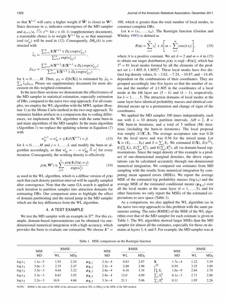
resentations. Since the target density of this example is a prod-uct of one-dimensional marginal densities, the above expec-tations can be calculated accurately through one-dimensionalnumerical integration. We compared our estimates from MDsampling with the results from numerical integration by com-puting mean squared errors (MSEs). We report the averageMSE of the estimated log probability masses (logλk) and theaverage MSE of the estimated conditional means (μX,k) overall the local modes at the same layer (k = 1, . . . ,5), and forother functions we only report the MSEs of the estimated ex-pectations to save space (Table 1).

As a comparison, we also applied the WL algorithm (as inthe naive two-step approach) to this problem with the same pa-rameter setting. The ratio (RMSE) of the MSE of the WL algo-rithm over that of the MD sampler for each estimate is given inTable 1. The WL algorithm showed larger MSEs than the MDsampler for almost all the estimates, especially for those on do-mains at layers 3, 4, and 5. For example, the MD sampler was at

Table 1. MSE comparison on the Rastrigin function

MSEMD

RMSEMSEMD

RMSEMSEMD

RMSE

WL MD0 WL MD0 WL MD0

logλ1 1.1e−5 1.93 2.24 μX,1 2.3e−4 0.83 2.87 X 1.7e−4 1.22 3.19logλ2 3.6e−3 2.35 2.47 μX,2 2.5e−4 2.88 2.96 e2S 0.59 3.25 3.09logλ3 3.5e−3 4.64 3.22 μX,3 2.8e−4 6.16 3.34

∏i Xi 1.6e−9 2.84 2.70

logλ4 3.3e−3 8.63 3.92 μX,4 2.9e−4 12.0 4.09∑

i X5i 6.1e−3 2.71 2.06

logλ5 3.2e−3 16.8 4.66 μX,5 3.3e−4 21.1 5.06∑

i X6i 0.11 1.95 2.26

NOTE: RMSE is the ratio of the MSE of the alternative method (WL or MD0) to the MSE of the MD method.

Zhou: Multi-Domain Sampler 1323

least 16 times more efficient than the WL algorithm for estimat-ing logλ5 and μX,5. The WL algorithm did not simulate suffi-cient samples from these domains, although it visited uniformlydifferent density partition intervals. On the contrary, the double-partitioning design facilitated the MD sampler to explore everydomain in a uniform manner, which led to a substantial im-provement in estimation for these layers. This shows the criti-cal role of domain partitioning in estimating DRs. To study theeffect of the mixed jump, we re-applied the MD sampler withpmx = 0, and calculated the ratio of the resulting MSE (MD0 inTable 1) over that of the MD sampler with pmx = 0.1, the de-fault setting. One sees an increase of two folds or more in MSEswithout the mixed jump. The convergence of the MD samplerwithout the mixed jump became slower, reflected by a five-fold increase in γn after the same number of iterations, averag-ing over 100 independent runs. These observations demonstratethat the mixed jump served as an efficient global move whichaccelerated convergence of the MD sampler and improved esti-mation accuracy.

5. LEARNING BAYESIAN NETWORKS

A Bayesian network (BN) factorizes the joint distribution ofm variables Z = {Z1, . . . ,Zm} into

P(Z) =m∏

i=1

P(Zi | �Gi ), (16)

where �Gi ⊂ Z is the parent set of Zi. A graph G is constructed

to code the structure of a BN by connecting each variable (node)to its child variables via directed edges. For (16) to be a well-defined joint distribution, the graph G must be a DAG. We con-sider the use of Bayesian networks in causal inference (Spirtes,Glymour, and Scheines 1993; Pearl 2000), which is tightly con-nected to many areas in statistics, such as structural equations,potential outcomes, and randomization (Rubin 1978; Robins1986; Holland 1988; Neyman 1990). Here we follow Pearl’sformulation of causal networks by modeling experimental in-tervention. If Zj is a parent of Zi in a causal Bayesian network,then experimental interventions that change the value of Zj mayaffect the distribution of Zi, but not conversely. Once all theparents of Zi are fixed by intervention, the distribution of Zi

will not be affected by interventions on any variables in the setZ \ (�G

i ∪ {Zi}). In the example causal network of Figure 2, ifwe fix Z1 and Z3 by experimental intervention, then the distri-bution of Z4 will not be affected by perturbations on Z2, Z5, orZ6.

Figure 2. An example Bayesian network of six variables.

5.1 Posterior Distribution

We focus on the discrete case where each Zi takes ri statesindexed by 1, . . . , ri and the parents of Zi take qi = ∏

Zj∈�Gi

rj

joint states. Let θijk be the causal probability for Zi = j giventhe kth joint state of its parent set. A causal BN with agiven structure G is parameterized by � = {θijk :

∑j θijk = 1,

θijk ≥ 0}.We infer network structure from two types of data jointly, ex-

perimental data and observational data. For experimental data,a subset of variables are known to be fixed by intervention. In-ferring causality with intervention has been extensively studiedin various contexts (e.g., Robins 1986, 1987; Pearl 1993). Weadopt the work of Cooper and Yoo (1999) for calculating theposterior probability of a network structure given a mix of ex-perimental and observational data. Suppose that Nijk is the num-ber of data points for which Zi is not fixed by intervention andis found in state j with its parent set in joint state k. Then, thecollection of counts N = {Nijk} is the sufficient statistic for �

(Ellis and Wong 2008). Let |�Gi | be the size of the parent set

of Zi. The prior distribution over network structures is specifiedas π(G) ∝ β

∑i |�G

i |, β ∈ (0,1), which penalizes graphs with alarge number of edges. With a product-Dirichlet prior for �,the posterior distribution [G | N] (Cooper and Herskovits 1992)is

P(G | N) ∝m∏

i=1

{β |�G

i |qi∏

k=1

[�(αi·k)

�(αi·k + Ni·k)

×ri∏

j=1

�(αijk + Nijk)

�(αijk)

]}, (17)

where αijk = α/(riqi) is the pseudo count for the causal proba-bility θijk in the product-Dirichlet prior and Ni·k = ∑

j Nijk (sim-ilarly for αi·k). The hyperparameters in the prior distributionsare chosen as β = 0.1 and α = 1.

5.2 MD Sampling Over DAGs

The space of DAGs is discrete in nature. We define domainsof attraction for P(G | N) (17) with a move set composed ofaddition, deletion, and reversal of an edge. Given a DAG Ga,we say that another DAG Gb is a neighbor of Ga if Gb can beobtained via a single move starting from Ga, that is, by adding,deleting, or reversing an edge of Ga. Denote by ngb(Ga) all theneighbors of Ga and let ngb(Ga) = ngb(Ga) ∪ {Ga}. A DAGG∗ is defined as a local mode of a probability density (mass)function p(G) if p(G∗) > p(G′) for every G′ ∈ ngb(G∗). Let G0

be a DAG and define recursively

Gt+1 = arg maxG∈ngb(Gt)

p(G), for t = 0,1, . . . . (18)

That is, we recursively find the single move that leads to thegreatest increase in p until a local mode is reached, which canbe viewed as a discrete counterpart of the gradient ascent al-gorithm. If there is more than one maximum in (18) with anidentical function value, we take the first maximum accordingto a fixed ordering of the neighbors. We call this recursion thesteepest neighbor ascent (SNA). Based on SNA, we define thedomain partition index I(G) and the attraction domains of p in

1324 Journal of the American Statistical Association, December 2011

the same manner as for a differentiable density [Equation (2)and Definition 1].

The target distribution in this application is the posterior dis-tribution P(G | N) and we define working density P(G | N;W)

similarly as in (6). To implement the MD sampler for DAGs,we employ the move set as the local proposal and develop thefollowing mixed jump. For a DAG G, we define an edge vari-able EG

ij for every pair of nodes Zi and Zj (i < j) such that

EGij = 1 if Zi is a parent of Zj, EG

ij = −1 if Zj is a parent

of Zi, and EGij = 0 otherwise. Given a DAG ν, let C(G;ν) =

(Ca(G;ν),Cd(G;ν),Cr(G;ν)) be a map of G, where

Ca(G;ν) =∑i<j

1(EGij �= 0,Eν

ij = 0),

Cd(G;ν) =∑i<j

1(EGij = 0,Eν

ij �= 0),

Cr(G;ν) =∑i<j

1(EGij · Eν

ij = −1).

In words, C(G;ν) gives the numbers of additions, deletions,and reversals needed to obtain G from ν. Let T = m(m − 1)/2be the total number of node pairs and |Eν | be the number ofedges in ν. Then, the number of common edges between G andν is |Eν | − [Cr(G;ν)+ Cd(G;ν)] and the number of node pairswith no edge in either DAG is T − |Eν | − Ca(G;ν). Given a setof local modes of P(G | N), {νk}M

k=1, let gk(G) = C(G;νk) in theupdate of Vt

k (8) of Algorithm 1, where Vtk = (vt

k,a, vtk,d, vt

k,r) is

a vector. As n → ∞, Vnk

a.s.−→ E[C(G;νk) | G ∈ Dk], where theexpectation is taken with respect to the limiting working den-sity P(G | N;W∗) (10). In the mixed jump, after a local modeνk is randomly chosen, we sequentially modify the edge vari-ables of νk to propose a new DAG Y . The proposal is designedaccording to Vt

k, the current estimate of the expected numbersof additions, deletions, and reversals of DAGs in the domainDk relative to the mode νk. Let |Ek| be the number of edges inνk. If Eνk

ij �= 0, we propose to reverse, delete, or retain the edge

Eνkij (i.e., EY

ij = −Eνkij ,0,or Eνk

ij ) with probabilities proportionalto the vector (vt

k,r, vtk,d, |Ek| − (vt

k,r + vtk,d)) + b, where b > 0

is a small prior count added to each category. Analogously, ifEνk

ij = 0 we propose EYij = 0,1,or − 1 with probabilities pro-

portional to (T −|Ek|− vtk,a, vt

k,a/2, vtk,a/2)+ b. Last, to ensure

a proposed graph is acyclic, a check for cycles is performedwhen we propose to add or reverse an edge in either the localproposal or the mixed jump. If the resulting graph is cyclic, wesuppress the probability for the corresponding move.

Following the common practice in structural learning of dis-crete BNs, we set an upper bound for the number of parents(indegree) of a node. In all the following examples and appli-cations, this upper bound is chosen to be four. We are inter-ested in the posterior expected adjacency matrix A = (aij)m×m

and its domain-based representation, where aij (1 ≤ i, j ≤ m) isthe posterior probability for a directed edge from Zi to Zj. Foreach identified local mode νk, we estimate the probability massλk of its attraction domain Dk and the conditional expectedadjacency matrix Ak on the domain. Then, A is estimated byA = ∑

k λkAk.

5.3 Simulation

We simulated data from two BNs, each of six binary vari-ables (m = 6, ri = 2,∀i). This is the maximum number of nodesfor which we can enumerate all DAGs, numbering about fourmillion, to obtain true posterior distributions and domain-basedrepresentations as the ground truth for testing a computationalmethod. The first network has a chain structure in which Zi isthe only parent of Zi+1 for i = 1, . . . ,5 and Z1 has no parent.The second network has a more complex structure shown inFigure 2. We simulated 50 datasets independently from eachnetwork. In each dataset, 20% of the data points were generatedwith interventions. Please see supplementary document for datasimulation details.

The MD sampler was applied to the 100 datasets with L = 15,H = 10, pmx = 0.1, K∗ = 100, and a total of 5M iterationswith the first 50K as burn-in iterations. To verify its perfor-mance, we compared identified local modes, estimated proba-bility masses {log λk}, conditional expected adjacency matrices{Ak}, and expected adjacency matrix A to their respective truevalues obtained via enumerating all DAGs. Our enumerationconfirms that the posterior distributions indeed have multiplelocal modes. The chain and the graph (Figure 2) networks haveon average 3.57 and 7.06 modes over the simulated datasets,respectively, and the maximum number of modes is 29 for thechain and 34 for the graph. As reported in Table 2, the MDsampler did not miss a single local mode for any dataset, whichdemonstrates its global search ability. Recall that all recordedmodes are detected in the burn-in algorithm. In fact, all modes,including the global mode, were identified within 10K itera-tions for every dataset. This observation confirms the notionthat the burn-in algorithm alone may serve as a powerful op-timization algorithm (Remark 4). We calculated the MSE ofthe vector (log λ1, . . . , log λK), where K is the number of localmodes, and the average MSE of A1, . . . , AK . When calculatingthe MSE of the log probability vector, we ignored those tinydomains with a probability mass < 10−4. These estimates areseen to be very accurate as reported in Table 2.

We also applied the MD sampler with pmx = 0 (MD0) andthe WL algorithm with the same parameter setting to thesedatasets (Table 2). The degraded performance of MD0 demon-strates the effectiveness of the mixed jump for sampling DAGs.

Table 2. Comparison on simulated data from two BNs

MDMSE

MD0 WL K∗ = 10

RMSE

# of missed modes 0 0 0 0.51log λk 0.028 1.48 5.06 0.48Ak 1.3e−4 1.65 11.0 0.99A 1.3e−4 1.76 1.67 1.03

# of missed modes 0 0 0.12 2.06log λk 0.029 401 1368 0.84Ak 1.7e−4 2.96 13.6 1.01A 1.5e−4 7.17 5.09 0.98

NOTE: The top and bottom panels report the results for the chain and the graph networks,respectively. For each estimate, reported are the MSE of the MD sampler and the RMSEs(ratios) of the other methods relative to the MD sampler.

Zhou: Multi-Domain Sampler 1325

The WL algorithm missed 0.12 modes on average for the sec-ond network, and its estimation of the DR {(Ak, λk)} was muchless accurate compared to that of the MD sampler. The aver-age MSE of A1, . . . , AK and the MSE of (log λk)1:K were morethan 10 and 1000 times greater than those of the MD sampler,respectively. The huge MSE of the (log λk) constructed by theWL algorithm was often due to severe underestimation of theprobability masses of domains sampled insufficiently. This re-sult implies that without domain partitioning, the WL algorithmis unable to estimate domain-based representations for a BN ofa moderately complicated structure. Since the number of localmodes often increases very fast with the complexity of a prob-lem, we re-applied the MD sampler with K∗ = 10 to investigatethe effect of keeping only a subset of local modes. Obviously,the algorithm missed a few local modes when the total numberof modes exceeded K∗. But in terms of estimating A and Ak,the performance of the MD sampler with K∗ = 10 was verycomparable to its performance when all the local modes werekept (Table 2). The probability mass outside the domains ofrecorded modes, λ0 = 1 − ∑K∗

k=1 λk, is less than 0.007 averag-ing over the 15 datasets where the posterior distributions havemore than 10 local modes. This confirms that the MD samplerindeed captured major modes in the burn-in period.

6. PROTEIN–SIGNALING NETWORKS

6.1 Background and Data

The ability of cells to properly respond to environment isthe basis of development, tissue repair, and immunity. Such re-sponse is established via information flow along signaling path-ways mediated by a series of signaling proteins. Cross-talks andinterplay between pathways reflect the network nature of theinteraction among these signaling molecules. Construction ofsignaling networks is an important step toward a global under-standing of normal cellular responses to various environmen-tal stimuli and more effective treatment of complex diseasescaused by malfunction of components in a pathway. CausalBayesian networks may be used for modeling signaling net-works as the relation among pathway components has a naturalcausal interpretation. That is, the activation or inhibition of a setof upstream molecules in a network causes the state change ofdownstream molecules. An edge from molecule A to moleculeB in a signaling network implies that a change in the state ofA causes a change in the state of B via a direct biochemicalreaction. Here, a state change refers to a chemical, physical, orlocational modification of a molecule. However, as there mayexist mutual regulation between two signaling molecules, theuse of DAGs for modeling signaling networks is only a first-step approximation.

In this study, we construct protein-signaling networks fromflow cytometry data. Polychromatic flow cytometry is a high-throughput technique for probing simultaneously the (phospho-rylation) states of multiple proteins in a single cell. Since mea-surements are collected on a cell-by-cell basis, huge amountsof data can be produced in one experiment. Sachs et al. (2005)made flow cytometry measurements of 11 proteins and phos-pholipids in the signaling network of human primary naiveCD4+ T cells under nine different experimental perturbationsthat either activate or inhibit a particular molecule or activate

Figure 3. An annotated protein-signaling network in naive CD4+T cells.

the entire pathway. Note that a perturbation that activates or in-hibits a particular molecule is essentially an intervention on themolecule, so that causal structures of the underlying networkmay be inferred. Under each perturbation, 600 cells were col-lected with 11 measurements for each. The measurements inthe data were discretized into three levels, high, medium, andlow by Sachs et al. In summary, this dataset contains 5400 datapoints for 11 ternary variables. Since naive T cells are essen-tial for the immune system to continuously respond to unfa-miliar pathogens, extensive studies have been conducted to es-tablish the signaling pathways. An annotated signaling networkamong the 11 molecules, provided by Sachs et al., is depictedas a causal Bayesian network in Figure 3. This network con-tains 18 edges that are well-established in the literature and twoedges (PKC → PKA and Erk → Akt) reported from recent ex-periments independent of the flow cytometry data.

6.2 Predicted Networks

The MD sampler was applied to this dataset with L = 20,H = 10, pmx = 0.1, and K∗ = 10. The total number of it-erations was 5M, of which the first 50K were used for burn-in. We estimated the posterior expected adjacency matrix Aand its domain-based representation. Three predicted networkswere constructed by thresholding posterior edge probabilities at

Table 3. Results on the flow cytometry data

MD MD0 WL

Global max (SD) −31,757.9 (2.7) −31,787.3 (82) −31,937.8 (199)TP/FP (c = 0.5) 15.50/10.35 15.55/10.35 13.40/12.35TP/FP (c = 0.7) 15.50/10.35 15.55/10.35 13.35/12.25TP/FP (c = 0.9) 15.50/10.35 15.55/10.35 13.35/11.95

TP/FP (c = 0.5) 15.2/10.3 14.6/10.6 11.6/13.6TP/FP (c = 0.7) 15.2/10.2 14.6/10.6 11.6/13.2TP/FP (c = 0.9) 15.2/9.9 14.6/10.2 11.6/13.1Log pred (mean) 0 −1.4 −62.1Log pred (DR) 17.5 16.2 −51.7

NOTE: The top and bottom panels report the average results over 20 independent runson the full dataset and the average results over ten test datasets in cross-validation, re-spectively. Predictive probabilities (Log pred) are reported as log ratios over the predictiveprobability given the mean network of the MD sampler.

1326 Journal of the American Statistical Association, December 2011

c = 0.5,0.7,0.9, that is, an edge from Zi to Zj was predicted ifthe edge probability aij ≥ c. For simplicity we call such a pre-dicted network a mean network (with a threshold c). Table 3(top panel) reports the number of true positive edges (TP) thatare both predicted by the MD sampler and annotated in Figure 3and the number of false positive edges (FP) that are predictedbut not annotated, together with the (unnormalized) log pos-terior probability of the identified global maximum DAG. Tocompare the results, we re-applied the MD sampler with thesame parameters except that pmx = 0 (MD0 in Table 3) and ap-plied the WL algorithm with the same parameters as used inthe MD sampler to the same data. The average result over 20independent runs of each method is summarized in Table 3. Interms of finding the global mode, the MD sampler was muchmore effective and robust than the other two algorithms, re-flected by a much higher average log probability and a muchsmaller standard deviation across multiple runs. The MD sam-pler with or without the mixed jump showed comparable resultsin predicting network structures, and both predicted more truepositives and fewer false positives than the WL algorithm didfor all the three thresholds. We noticed that the mean networksconstructed with different thresholds (c = 0.5,0.7,0.9) were al-most identical. This was due to the fact that the posterior edgeprobabilities were close to either 1 or 0 because of the largedata size. The network constructed from the same data by theorder-graph sampler, reported in figure 11 of the article by El-lis and Wong (2008), has 9 true positive and 11 false positiveedges, which misses many more true edges and includes morefalse positives than the networks predicted by the MD sampler.These results demonstrate that the MD sampler is very power-ful in learning underlying network structures from experimentaldata compared to other advanced Monte Carlo techniques.

Next, we focus on the estimation of the DR, {(Ak, λk) : k =0, . . . ,K∗}, and its scientific implications. A network Gk canbe constructed for an attraction domain by thresholding Ak, theconditional expected adjacency matrix on the domain Dk, fork = 1, . . . ,K∗. To distinguish it from the mean network, we callGk a local network. We take the result of a representative run ofthe MD sampler (pmx = 0.1) to demonstrate local networks withthe threshold c = 0.9. The parent sets of eight nodes are iden-tical across the K∗ = 10 local networks. We report in Table 4the parents of the other three nodes, PLC, PIP3, and Erk, which

are distinct among the local networks, together with the prob-ability masses (log λk) of the 10 domains and the probabilitiesof the local modes [log P(νk | N)]. The local networks may pre-dict meaningful alternative edges not included in the mean net-work, as illustrated by the result on a particular pathway, Raf →Mek → Erk (Figure 3). This expected pathway was predictedby all the local networks and the mean network. However, somelocal networks also contained a direct link from Raf to Erk (Ta-ble 4). As Mek was inhibited in one of the experimental con-ditions, this finding suggests that the cells may have anotherpathway that passes the signal from Raf to Erk via some indirectregulation or via molecules not included in this analysis, whenMek is not functioning properly. Such compensational mech-anisms exist widely in many biological networks. Indeed, Rafhas been reported to enhance the kinase activity of PKCθ , anisoform of PKC, although PKCθ is unlikely a direct phospho-rylation target of Raf (Hindley and Kolch 2007). As indicatedby Figure 3, Erk is a downstream node of PKC and thus may beregulated indirectly by Raf via the enhanced kinase activity ofPKCθ . Such novel hypotheses could not be proposed if we didnot construct the DR for the posterior distribution. Clearly, theDR of network structures not only gives a detailed landscape ofvarious local domains but also provides new insights into theunderlying scientific problem.

From Table 4 we find that the probability mass is dominatedby the domain of the identified global mode with a log prob-ability of −31,757. Consistent with the summary in Table 3,the MD sampler almost always reached this global mode fordifferent runs. On the contrary, the highest mode detected bythe WL algorithm with an average log probability of −31,938is even much lower than the lowest mode in Table 4. In otherwords, the WL algorithm was inevitably trapped to some localmodes with negligible probability masses. This again demon-strates the advantage of the MD sampler, particularly the burn-in algorithm, in finding global modes. Even when the proba-bility mass of the global mode is dominant and other domainsoccupy only a small fraction of the sample space, without thedomain-partitioning design the WL algorithm may be trappedto a local mode of a tiny probability mass and produce severelybiased estimates.

6.3 Cross-Validation

To check the statistical variability and the predictive powerof our method, we conducted ten-fold cross-validation on this

Table 4. Local networks constructed from domain-based representation

Parents of

log λk log P(νk | N) PLC PIP3 Erk

−0.00274 −31,756.81 PKC p38 JNK PLC PKC Mek PKA PKC−6.39777 −31,762.75 PKC p38 JNK PLC PKC Mek PKA Raf−7.12166 −31,764.16 Mek PKA PLC PKC Mek PKA PKC−8.34521 −31,764.82 PKC p38 JNK PLC JNK Mek PKA PKC

−10.6461 −31,766.81 Mek Akt p38 PLC PKC Mek PKA PKC−13.7193 −31,770.11 Mek Akt PKA PLC PKC Mek PKA Raf−14.0777 −31,770.77 PKC p38 JNK PLC JNK Mek PKA Raf−15.0459 −31,772.18 Mek Akt PKA PLC JNK Mek PKA PKC−16.8860 −31,772.76 Mek Akt p38 PLC PKC Mek PKA Raf−18.5716 −31,774.82 Mek Akt p38 PLC JNK Mek PKA PKC

Zhou: Multi-Domain Sampler 1327

dataset. We partitioned randomly the 5400 data points into tensubsets of equal sizes. We used nine subsets as training datato learn a mean network and calculated the predictive proba-bility of data points in the other subset (test data) given thelearned mean network. This procedure was repeated 10 timesto test on every subset. We verified the average accuracy of themean networks constructed from the 10 training datasets withdifferent thresholds. The performance of the MD sampler on thetraining datasets was comparable to its performance on the fulldataset, which implies its robustness to random sampling of in-put data. The improvement in accuracy (TP/FP) of the MD sam-pler over the other two methods became more significant, espe-cially compared to the WL algorithm (Table 3, bottom panel).The average predictive probability of the test datasets given themean networks constructed from the training datasets by eachmethod with c = 0.9 is reported in Table 3 [Log pred (mean)],from which we see that the predictive power of the networksconstructed by the two MD samplers was much higher than thatof the WL algorithm (> 60 in log probability ratio). In addition,we utilized the estimated domain-based representations to cal-culate the predictive probability of a test data point y by

P(y | {Gk, λk}) =K∗∑

k=0

λkP(y | Gk), (19)

where P(y | Gk) is the marginal likelihood of y given the localnetwork Gk. This can be regarded as a domain-based approxi-mation to the posterior predictive distribution

P(y | yobs) =∑

G

P(G | yobs)P(y | G),

that is, we use estimated probability masses λk and conditionalmean networks Gk to approximate the posterior predictive prob-ability. The advantage is that there is no need to store a largeposterior sample of networks but only an estimated DR. SinceEquation (19) captures the variability among different domains,it is expected to outperform the mean network in prediction. Infact, for each method the predictive probability calculated by(19) [Table 3, Log pred (DR)] was indeed significantly greaterthan the predictive probability calculated given its mean net-work, especially for the two MD samplers.

In real applications, we are interested in predicting resultsfor a new experimental condition given observed data fromother conditions. Thus, we also performed a nine-fold cross-validation where a training dataset was composed of cells fromeight experimental conditions and a test dataset only includedcells in the other one condition. We applied the MD sampler toconstruct mean networks and DRs {Gk, λk}10

k=1 from the trainingdatasets. The mean networks with c = 0.9 included, on average,13.2 true edges with 10.8 false edges, which was slightly worsethan the result from the ten-fold cross-validation. The degradedperformance is expected as removing all cells from one experi-mental perturbation will increase the uncertainty in determiningthe directionality of the network. The domain-based prediction(19) was compared against the annotated network G∗ given inFigure 3, which presumably has the highest predictive power,by evaluating the log-likelihood ratio (LLR) log R = log[P(y |{Gk, λk})/P(y | G∗)], where y is a test data point. The average

log R over all test data points was −0.062, and thus the predic-tive probability for a new observation given the constructed DRis expected to be higher than 94%(= e−0.062) of its likelihoodgiven the annotated graph. This demonstrates the high predic-tive power of the domain-based prediction constructed by ourmethod. As expected, the average LLR of the mean networksover G∗ was 26% lower than the average of log R.

7. DISCUSSION

The central idea of this article is to construct domain-basedrepresentations with the MD sampler. Related works have beenseen in the physics literature under the name of superposi-tion approximation. Please see the article by Wales and Bog-dan (2006) for a recent review. Given a Boltzmann distributionpB(x; τ) ∝ exp[−H(x)/τ ], a superposition approach identifiesthe local minima of H(x), that is, the local modes of pB(x; τ),and approximates H(x) on the attraction domain of a local min-imum by quadratic or high-order functions. The approximationis often proposed based on expert knowledge about the physicalmodel under study. Expectations with respect to pB(x; τ) arethen estimated by summing over approximations from identi-fied domains. The accuracy of this approach largely depends onthe employed approximation to H(x) on a domain and thus maynot work well for an arbitrary distribution. The MD samplerdiffers in that domain-based representations are constructed byMonte Carlo sampling which is able to provide accurate estima-tion with large-size samples; no expert knowledge about the tar-get distribution is needed. In addition, our method also containsa coherent component for finding local modes, while the super-position approximation works more like a two-step approach.

From a computational perspective, the MD sampler inte-grates Monte Carlo and deterministic optimization. A few othermethods also have the two ingredients, such as Monte Carlooptimization (Li and Scheraga 1987), the basin hopping algo-rithm (Wales and Doye 1997), and conjugate gradient MonteCarlo (CGMC) (Liu, Liang, and Wong 2000). In Monte Carlooptimization and the basin hopping algorithm, the target distri-bution p(x) is modified to p(x) = p(νk) for all x ∈ Dk, where Dk

is the attraction domain of the mode νk. Then a Metropolis-typeMCMC is used to sample from p, in which a local optimiza-tion algorithm is employed at each iteration to find p(Xt) forthe current state Xt. These methods have been applied to iden-tification of minimum-energy structures of proteins and othermolecules. However, its application to other fields is limitedas the modified density p(x) may be improper when the sam-ple space is unbounded. In CGMC, a population of samples isevolved and a line sampling step (Gilks, Roberts, and George1994) is performed on a sample along a direction pointing to alocal mode found by local optimization initiated at another sam-ple. In this way promising proposal may be constructed by bor-rowing local mode information from other samples. A possiblefuture work on the MD sampler is to utilize a population of sam-ples. Because local modes are recorded, similar proposals as theline sampling can be developed for the MD sampler to furtherenhance sampling effectiveness. Another future direction is toconstruct disconnectivity graphs (Becker and Karplus 1997) ortrees of sublevel sets (Zhou and Wong 2008) from samples gen-erated by the MD sampler. Since samples have been partitioned

1328 Journal of the American Statistical Association, December 2011

into domains of attraction, we only need to determine the bar-rier between a pair of domains, defined by maxs∈S minx∈s p(x),where S is the collection of all the paths between the two do-mains. A few candidate approaches toward this direction areunder current investigation (Zhou 2011).

APPENDIX: THEORETICAL ANALYSIS

In this appendix we establish the convergence and ergodicity prop-erties of the MD sampler. Our analysis is conducted for a doubly adap-tive MCMC, that is, both the target distribution and the proposal maychange along the iteration, which includes the MD sampler as a spe-cial case. Furthermore, the MWL design (Routine 1) is employed toadjust γt .

Assume that the sample space X is equipped with a countably gen-erated σ -field, B(X ). Let {Xi}κi=1 be a partition of X , where each Xiis nonempty, and B(Xi) = {A ∈ B(X ) : A ⊆ Xi} for i = 1, . . . , κ . Letω = (ωi)1:κ ∈ � and φ ∈ � be two vectors of real parameters. Denotethe product parameter space by � = � × � and write θ = (ω,φ) ∈ �.For ω ∈ �, define working density

pω(x) ∝κ∑

i=1

e−ωi p(x)1(x ∈ Xi). (A.1)

Let q(x, ·) and tφ(x, ·), φ ∈ �, be two transition kernels on (X , B(X )).Hereafter, the same notation will be used for a kernel and its densitywith respect to the Lebesgue measure on X , for example, q(x, dy) ≡q(x,y)dy. For j = 0,1, define Qj,φ(x, ·) = (1− j)q(x, ·)+ jtφ(x, ·). LetKj,θ be the MH transition kernel with pω as the target distribution andQj,φ as the proposal, that is,

Kj,θ (x,dy) = Sj,θ (x,dy) + 1(x ∈ dy)

[1 −

∫X

Sj,θ (x,dz)],

where Sj,θ (x,dy) = Qj,φ(x,dy)min[1,pω(y)Qj,φ(y,x)/pω(x)Qj,φ(x,

y)], representing an accepted move. As Q0,φ = q, K0,θ and S0,θ donot depend on φ and thus reduce to K0,ω and S0,ω , respectively.Furthermore, if we let ω = 0, then pω(x) = p(x), in which case wesimply use K0 and S0. Given α ∈ [0,1), define a mixture proposalQφ = (1−α)q+αtφ , its accepted move Sθ = (1−α)S0,ω +αS1,θ , andthe corresponding MH kernel Kθ = (1 − α)K0,ω + αK1,θ . Table A.1summarizes the notations, from left to right, for target distributions,proposals, MH kernels, and accepted moves for different scenarios in-volved in this analysis.

Denote by Z(ω) the normalizing constant of (A.1). Then Z(ω) =∑κi=1 Zi(ωi), where Zi(ωi) = e−ωi

∫Xi

p(x)dx. Let U be a nonemptysubset of {1, . . . , κ} and XU = ⋃

i∈U Xi. Given a map g : X → �,let μg,U(ω) = E[g(X) | X ∈ XU] with respect to pω . Define a mapH :� × X → � by

H(θ ,x) = [(1(x ∈ Xi) − 1/κ

)1:κ , (g(x) − φ)1(x ∈ XU)

]and the mean field F(θ) = ∫

X H(θ,x)pω(x)dx, that is,

F(θ) =[(

Zi(ωi)

Z(ω)− 1

κ

)1:κ

,

∑u∈U Zu(ωu)

Z(ω)(μg,U(ω) − φ)

].

Consider the equation F(θ) = 0. Let ω∗ = [log Zi(0)]1:κ and φ∗ =μg,U(ω∗). As F(θ) is invariant to translation of ω by a scalar: ω →(ω + β)

= (ωi + β)1:κ , β ∈ R, the solution set to this equation is

Table A.1. Summary of notations

Mixture: pω Qφ Kθ Sθ

j = 0: pω q K0,ω S0,ω

j = 0,ω = 0: p q K0 S0j = 1: pω tφ K1,θ S1,θ

{θ∗(β)= (ω∗ + β,φ∗)} ∩ �

= �∗. Set γ1 = 1 and choose an arbi-trary point (x, θ) ∈ X × � to initialize (X1, θ1). A doubly adaptiveMCMC is employed to find a solution θ∗(β) ∈ �∗ and to estimateμh(ω∗) = ∫

X h(x)pω∗(x)dx for a function h : X → R.

Algorithm A.1 (Doubly adaptive MCMC). Choose a fixed α ∈[0,1). For t = 1, . . . ,n:

1. If θ t /∈ �, set Xt+1 = x and θ t+1 = θ ; otherwise draw Xt+1 ∼Kθ t (Xt, ·) and set θ t+1 = θ t + γtH(θ t,Xt+1).

2. Determine γt+1 by the MWL design in Routine 1 with {Xi} inplace of {Dkj}.

Denote the L2 norm by | · | and let d(x,A)= infy∈A |x − y|, where

x,y are vectors and A is a set. Our goal is to establish that d(θn,�∗) →0 almost surely (with respect to the probability measure of the process{Xt, θ t}) and that {Xt} is ergodic. Clearly, translation of ωt by a scalardoes not change the working density pωt or affect the convergence ofθ t to �∗. Thus, the theory for Algorithm A.1 can be applied to theMD sampler with reinitialization (Remark 2). The update of ωt , up totranslation by a scalar, and the update of φt correspond to, respectively,the update of Wt (7) and the update of Vt

k (8) for any k in the MDsampler. We state four conditions for establishing the main results.

(C1) The sample space X is compact, p(x) > 0 for all x ∈ X , � isbounded, and �∗ is nonempty. The map g and the function hare p-integrable and bounded.

(C2) There exist δq > 0 and εq > 0 such that |x − y| ≤ δq impliesthat q(x,y) ≥ εq for all x,y ∈ X .

(C3) There exist an integer �, δ > 0 and a probability measure ν,such that ν(Xi) > 0 for i = 1, . . . , κ and S�

0(x,A) ≥ δν(A),∀x ∈ X and A ∈ B(X ).

(C4) For all x,y ∈ X and all φ ∈ �, tφ(x,y) > 0 and log tφ(x,y)

has continuous partial derivatives with respect to all the com-ponents of φ.

To avoid mathematical complexity, we assume that X is compact(C1). This assumption does not lose much generality in practice as wemay always restrict the sample space to {x : p(x) ≥ εp} given a suf-ficiently small εp. Due to the compactness of X , any continuous mapand function on X will be bounded. Conditions (C2), (C3) are standardconditions on the fixed proposal q(x,y) to guarantee irreducibility andaperiodicity of the MH kernel K0. They are satisfied by all the localmoves used in this article. A regularity condition on the adaptive pro-posal tφ is specified in (C4). For the mixed jumps in the examples, φ

is either the covariance matrix of a multivariate normal distribution orthe cell probability vector of a multinomial distribution, and (C4) issatisfied.

Lemma A.1. Let α ∈ [0,1). For any i, j ∈ {1, . . . , κ} and θ ∈ �, ifeωi−ωj ≥ c1 ∈ (0,1], then Kθ (x,A) ≥ (1 − α)c1S0(x,A), ∀x ∈ Xi andA ∈ B(Xj).

Proof. By definition, Kθ (x,A) ≥ (1 − α)K0,ω(x,A) ≥ (1 − α) ×S0,ω(x,A) for every θ = (ω,φ). For any x ∈ Xi and y ∈ Xj,

S0,ω(x,dy) = q(x,dy)min

[1, eωi−ωj

p(y)q(y,x)

p(x)q(x,y)

]

≥ c1q(x,dy)min

[1,

p(y)q(y,x)

p(x)q(x,y)

]= c1S0(x,dy).

Thus, Kθ (x,A) ≥ (1 − α)c1S0(x,A) for all A ∈ B(Xj).

Theorem A.1. If (C1)–(C4) hold, then d(θn,�∗)a.s.−→ 0 and

1

n

n∑t=1

h(Xt)a.s.−→ μh(ω∗), as n → ∞. (A.2)

Zhou: Multi-Domain Sampler 1329

Proof. Lemma A.1 and (C3) imply that ∀x ∈ Xi, K�θ (x, Xj) ≥

ενν(Xj) > 0 if eωi−ωj ≥ c1, where εν > 0. By Theorem 4.2 of thearticle by Atchadé and Liu (2010),

maxi,j

lim supn→∞

|vni − vn

j | < ∞, a.s.,

where vni = ∑n

t=1 1(Xt ∈ Xi). This implies that the {γt} defined by theMWL update (Routine 1) will decrease below any given εγ > 0 af-ter a finite number of iterations, that is, tc < ∞, almost surely. Then,Algorithm A.1 becomes a stochastic approximation algorithm with adeterministic sequence of {γt}. According to proposition 6.1 and the-orem 5.5 in the article of Andrieu, Moulines, and Priouret (2005), weonly need to verify the drift conditions (DRI1–3) and assumptions(A1), (A4) given in that work to show the convergence of θn.

Verifying the drift conditions. Let D be any compact subsetof �, and D1 and D2 be the projections of D into � and �, re-spectively. Since D1 is compact, there is an εD ∈ (0,1] such thatmini,j infω∈D1

eωi−ωj ≥ εD . By Lemma A.1 and (C3), there is aδD > 0 such that

infθ∈D

K�θ (x,A) ≥ δDν(A), ∀x ∈ X ,A ∈ B(X ), (A.3)

where � and ν are defined in (C3). This gives the minorization con-dition in (DRI1). Given (C2) and that pω,ω ∈ D1, is bounded awayfrom 0 and ∞ under (C1), K0,ω is irreducible and aperiodic for ev-ery ω ∈ D1, according to theorem 2.2 of the article by Roberts andTweedie (1996). Consequently, for every θ ∈ D, Kθ is also irreducibleand aperiodic as α < 1. Let V(x) = 1 for all x ∈ X . It is then easy toverify other conditions in (DRI1).

Since both g and � are bounded (C1), there is a c2 > 0 such that forall x ∈ X ,

supθ∈�

|H(θ ,x)| ≤ κ + |g(x)| + supφ∈�

|φ| ≤ c2, (A.4)

|H(θ ,x) − H(θ ′,x)| ≤ |φ − φ′| ≤ c2|θ − θ ′|, ∀θ , θ ′ ∈ �. (A.5)

These two inequalities imply (DRI2) with V(x) = 1.Condition (DRI3) can be verified by the same argument used by

Liang, Liu, and Carroll (2007) once we find a constant c3 > 0 suchthat ∣∣∣∣∂Sθ (x,y)

∂θi

∣∣∣∣ ≤ c3Qφ(x,y), (A.6)

for all x,y ∈ X , θ ∈ D, and all i, where θi is the ith component ofθ = (ω,φ). Denote by φj the jth component of φ. Straightforward cal-culation leads to |∂Sθ (x,y)/∂ωi| ≤ Qφ(x,y) and

∂Sθ (x,y)

∂φj=

⎧⎪⎪⎨⎪⎪⎩

Rθ (x,y)[∂ log tφ(y,x)/∂φj]αtφ(x,y),

if Rθ (x,y) < 1

[∂ log tφ(x,y)/∂φj]αtφ(x,y),

otherwise,

where Rθ (x,y) = pω(y)tφ(y,x)/pω(x)tφ(x,y). Condition (C4) withthe compactness of D2 and X guarantees that

supx,y∈X

supφ∈D2

|∂ log tφ(x,y)/∂φj| < ∞.

As αtφ(x,y) ≤ Qφ(x,y), (A.6) holds and (DRI3) is verified.Verifying assumptions (A1), (A4). It is assumed in assumption (A1)

the existence of a global Lyapunov function for F(θ). Let L(θ) =c42

∑κi=1(Zi(ωi)− Z(ω))2 + 1

2 |φ −μg,U(ω)|2, where Z(ω) = Z(ω)/κ .Using straightforward algebra one can show that

−Z〈∇L,F〉 =κ∑

i=1

c4Zi · (Zi)2

+ (φ)T∑u∈U

Zu∂μg,U(ω)

∂ωu+

∑u∈U

Zu|φ|2,

where Zi = Zi(ωi) − Z(ω), φ = φ − μg,U(ω), and the arguments(ωi and ω) in Zi(ωi) and Z(ω) have been dropped. Since � is bounded,Zi(ωi) > ε� > 0 for all i. Because g is p-integrable, μg,i

= μg,{i}(0)

is bounded for all i and∣∣∣∣∂μg,U(ω)

∂ωu

∣∣∣∣ ≤ |μg,u| + maxi∈U

|μg,i| ≤ 2 max1≤i≤κ

|μg,i| < ∞.

Thus, choosing a sufficiently large c4 ensures that 〈∇L(θ),F(θ)〉 ≤0 for any θ ∈ � with equality if and only if θ ∈ �∗. Furthermore,{θ ∈ � : L(θ) ≤ CL} is compact for some CL > 0 and the closure ofL(�∗) has an empty interior. Thus, all the conditions in assumption(A1) are satisfied. Since |θ t+1 − θ t| ≤ γt supθ ,x |H(θ,x)| ≤ c2γt (A.4)and γt = 1/(t + ξ) for t > tc, verifying assumption (A4) is immediate.This completes the proof of the convergence of θn.

The result (A.2) can be established similarly as the proof of propo-sition 6.2 in the work of Atchadé and Liu (2010). We only give anoutline here. The drift conditions imply that for any θ ∈ D, there existhθ (x), c5 > 0, and b ∈ (0,1] such that hθ − Kθ hθ = h − μh(ω) and

supθ∈D

(‖hθ‖ + ‖Kθ hθ‖) < ∞,

‖hθ − hθ ′ ‖ + ‖Kθ hθ − Kθ ′hθ ′ ‖ < c5|θ − θ ′|b, ∀θ , θ ′ ∈ D,

where Kθ hθ (x) = ∫X Kθ (x,dy)hθ (y) and for f : X → R, ‖f ‖ =

supx∈X |f (x)|. See Proposition 6.1 and assumption (A3) in the workof Andrieu, Moulines, and Priouret (2005). Then, following an essen-tially identical proof to that of lemma 6.6 in the work of Atchadé andLiu (2010), we can show that

∑∞t=1 t−1[h(Xt+1)−μh(ωt)] has a finite

limit almost surely. Since μh(ωt)a.s.−→ μh(ω∗) as t → ∞, Kronecker’s

lemma applied to the above infinite sum leads to the desired result.

SUPPLEMENTARY MATERIALS

Supplement: The supplementary document contains (1) morediscussion on the weighted estimator in Section 3.3 and(2) data simulation details in Section 5.3.(MultiDomainSuppl_R5.pdf)

[Received May 2010. Revised June 2011.]

REFERENCES

Andrieu, C., and Moulines, E. (2006), “On the Ergodicity Properties of SomeAdaptive MCMC Algorithms,” Annals of Applied Probability, 16, 1462–1505. [1320]

Andrieu, C., Moulines, E., and Priouret, P. (2005), “Stability of Stochastic Ap-proximation Under Verifiable Conditions,” SIAM Journal of Control andOptimization, 44, 283–312. [1320,1329]

Atchadé, Y. F., and Liu, J. S. (2010), “The Wang–Landau Algorithm in GeneralState Spaces: Applications and Convergence Analysis,” Statistica Sinica,20, 209–233. [1317,1320,1321,1329]

Becker, O. M., and Karplus, M. (1997), “The Topology of MultidimensionalPotential Energy Surface: Theory and Application to Peptide Structure andKinetics,” Journal of Chemical Physics, 106, 1495–1517. [1327]

Chen, M. H., Shao, Q., and Ibrahim, J. G. (2001), Monte Carlo Methods inBayesian Computation. New York: Springer. [1317]

Cooper, G. F., and Herskovits, E. (1992), “A Bayesian Method for the Induc-tion of Probabilistic Networks From Data,” Machine Learning, 9, 309–347.[1323]

Cooper, G. F., and Yoo, C. (1999), “Causal Discovery From a Mixture of Ex-perimental and Observational Data,” in Proceedings of the 15th Conferenceon Uncertainty in Artificial Intelligence, San Francisco, CA: Morgan Kauf-mann, pp. 116–125. [1323]

Ellis, B., and Wong, W. H. (2008), “Learning Causal Bayesian Network Struc-tures From Experimental Data,” Journal of the American Statistical Associ-ation, 103, 778–789. [1318,1323,1326]

Friedman, N., and Koller, D. (2003), “Being Bayesian About Network Struc-ture: A Bayesian Approach to Structure Discovery in Bayesian Networks,”Machine Learning, 50, 95–126. [1318]

Gelfand, A. E., and Smith, A. F. M. (1990), “Sampling-Based Approaches toCalculating Marginal Densities,” Journal of the American Statistical Asso-ciation, 85, 398–409. [1317]

1330 Journal of the American Statistical Association, December 2011

Geman, S., and Geman, D. (1984), “Stochastic Relaxation, Gibbs Distributionsand the Bayesian Restoration of Images,” IEEE Transactions on PatternAnalysis and Machine Intelligence, 6, 721–741. [1317]

Geyer, C. J. (1991), “Markov Chain Monte Carlo Maximum Likelihood,” inComputing Science and Statistics: Proc. 23rd Symp. Interface, ed. E. M.Keramidas, Fairfax Station, VA, pp. 156–163. [1319]

Gilks, W. R., Roberts, R. O., and George, E. I. (1994), “Adaptive DirectionSampling,” The Statistician, 43, 179–189. [1327]

Gordon, V. S., and Whitley, D. (1993), “Serial and Parallel Genetic Algorithmsas Function Optimizers,” in Proc. 5th Int. Conf. Genetic Algorithms, SanMateo, CA, pp. 177–183. [1322]

Haario, H., Saksman, E., and Tamminen, J. (2001), “An Adaptive MetropolisAlgorithm,” Bernoulli, 7, 223–242. [1319]

Hastings, W. K. (1970), “Monte Carlo Sampling Methods Using MarkovChains and Their Applications,” Biometrika, 57, 97–109. [1317]

Hindley, A., and Kolch, W. (2007), “Raf-1 and B–Raf Promote Protein KinaseC θ Interaction With BAD,” Cellular Signalling, 19, 547–555. [1326]

Holland, P. W. (1988), “Causal Inference, Path Analysis, and Recursive Struc-tural Equations Models,” in Sociological Methodology, ed. C. C. Clogg,Washington, DC: American Sociological Association, pp. 449–484. [1323]

Li, Z., and Scheraga, H. A. (1987), “Monte Carlo-Minimization Approach tothe Multiple-Minima Problem in Protein Folding,” Proceedings of the Na-tional Academy of Sciences, USA, 84, 6611–6615. [1327]

Liang, F. (2005), “Generalized Wang–Landau Algorithm for Monte Carlo Com-putation,” Journal of the American Statistical Association, 100, 1311–1327.[1317]

(2009), “On the Use of Stochastic Approximation Monte Carlo forMonte Carlo Integration,” Statistics and Probability Letters, 79, 581–587.[1321]

Liang, F., and Zhang, J. (2009), “Learning Bayesian Networks for DiscreteData,” Computational Statistics and Data Analysis, 53, 865–876. [1318]

Liang, F., Liu, C., and Carroll, J. (2007), “Stochastic Approximation in MonteCarlo Computation,” Journal of the American Statistical Association, 102,305–320. [1317,1320,1329]

Liu, J. S. (2008), Monte Carlo Strategies in Scientific Computing (2nd ed.),New York: Springer. [1317]

Liu, J. S., Liang, F., and Wong, W. H. (2000), “The Multiple-Try Method andLocal Optimization in Metropolis Sampling,” Journal of the American Sta-tistical Association, 95, 121–134. [1327]

Metropolis, N., Rosenbluth, A. W., Rosenbluth, M. N., Teller, A. H., and Teller,E. (1953), “Equations of State Calculation by Fast Computing Machines,”Journal of Chemical Physics, 21, 1087–1091. [1317]

Neyman, J. (1990), “Sur les applications de la thar des probabilities aux expe-rience Agaricales: Essay des principle” [English translation of excerpts byD. Dabrowska and T. Speed], Statistical Science, 5, 463–472. [1323]

Pearl, J. (1993), “Graphical Models: Causality and Intervention,” StatisticalScience, 8, 266–273. [1323]

(2000), “The Logic of Counterfactuals in Causal Inference,” Journalof the American Statistical Association, 95, 428–435. [1323]

Roberts, G. O., and Tweedie, R. L. (1996), “Geometric Convergence and Cen-tral Limit Theorems for Multidimensional Hastings and Metropolis Algo-rithms,” Biometrika, 83, 95–110. [1329]

Robins, J. (1986), “A New Approach to Causal Inference in Mortality StudiesWith Sustained Exposure Periods: Application to Control of the HealthyWorker Survivor Effect,” Math Modeling, 7, 1393–1512. [1323]

(1987), “A Graphical Approach to the Identification and Estimation ofCausal Parameters in Mortality Studies With Sustained Exposure Periods,”Journal of Chronic Diseases, 40, 1395–1615. [1323]

Rubin, D. (1978), “Bayesian Inference for Causal Effects: The Role of Ran-domization,” The Annals of Statistics, 6, 34–58. [1323]

Sachs, K., Perez, O., Peer, D., Lauffenburger, D. A., and Nolan, G. P. (2005),“Causal Protein-Signalling Networks Derived From Multiparameter Single-Cell Data,” Science, 308, 523–529. [1325]

Spirtes, P., Glymour, C., and Scheines, R. (1993), Causation, Prediction, andSearch (2nd ed.), Cambridge, MA: MIT Press. [1323]

Tanner, M. A., and Wong, W. H. (1987), “The Calculation of Posterior Distri-butions by Data Augmentation,” Journal of the American Statistical Asso-ciation, 82, 528–550. [1317]

Wang, F., and Landau, D. P. (2001), “Efficient Multiple-Range Random-WalkAlgorithm to Calculate the Density of States,” Physical Review Letters, 86,2050–2053. [1317,1320]

Wales, D. J., and Bogdan, T. V. (2006), “Potential Energy and Free EnergyLandscapes,” Journal of Physical Chemistry B, 110, 20765–20776. [1327]

Wales, D. J., and Doye, J. P. K. (1997), “Global Optimization by Basin-Hoppingand the Lowest Energy Structures of Lennard–Jones Clusters Containing upto 110 Atoms,” Journal of Physical Chemistry A, 101, 5111–5116. [1327]

Zhou, Q. (2011), “Random Walk Over Basins of Attraction to Construct IsingEnergy Landscapes,” Physical Review Letters, 106, 180602. [1328]

Zhou, Q., and Wong, W. H. (2008), “Reconstructing the Energy Landscape ofa Distribution From Monte Carlo Samples,” Annals of Applied Statistics, 2,1307–1331. [1327]