multi label classification pedro...
TRANSCRIPT

Intro Metrics Methods Advanced Software Conclusions
MULTI-LABEL CLASSIFICATION
Pedro Larranaga
Computational Intelligence GroupArtificial Intelligence Department
Technical University of Madrid
V Simposio de Teorıa y Aplicaciones de Minerıa de Datos. TAMIDA’2010Valencia, September 9, 2010
P. Larranaga Multi-label Classification

Intro Metrics Methods Advanced Software Conclusions
Outline
1 Introduction
2 Evaluation Metrics
3 Methods for Learning Multi-label Classifiers
4 Advanced Topics
5 Software
6 Conclusions
P. Larranaga Multi-label Classification

Intro Metrics Methods Advanced Software Conclusions
Introduction. Single Label versus Multi-label
X1 X2 X3 X4 X5 C3.2 1.4 4.7 7.5 3.7 12.8 6.3 1.6 4.7 2.7 07.7 6.2 4.1 3.3 7.7 19.2 0.4 2.8 0.5 3.9 05.5 5.3 4.9 0.6 6.6 1
X1 X2 X3 X4 X5 C1 C2 C3 C43.2 1.4 4.7 7.5 3.7 1 0 1 12.8 6.3 1.6 4.7 2.7 0 0 1 07.7 6.2 4.1 3.3 7.7 1 0 1 19.2 0.4 2.8 0.5 3.9 0 1 0 05.5 5.3 4.9 0.6 6.6 1 1 0 1
P. Larranaga Multi-label Classification

Intro Metrics Methods Advanced Software Conclusions
Introduction. Text Categorization
ACM Computing Classification System (Veloso et al. 2007)Versions: 1964, 1991 and 1998 (valid until 2010)
A document is described by its title, abstract, citations, authorship (huge andsparse feature space)
First hierarchy level: 11 labelsGeneral literatureHardwareComputer systems organizationSoftwareDataTheory of computationMathematics of computingInformation systemsComputing methodologiesComputer applicationsComputing milieux
Second hierarchy level: 81 labels
81,251 digital library articles
P. Larranaga Multi-label Classification

Intro Metrics Methods Advanced Software Conclusions
Introduction. Text Categorization
Reuters Corpus Volume 1 (RCV1-v2) (Lewis et al. 2004)Automated indexing of a text804,414 newswire stories indexed by Reuters Ltd103 topic codes organized in a hierarchy (2.6 topics onaverage per story)350 industry codes (in a two level hierarchy) based on thetypes of business in the story
P. Larranaga Multi-label Classification

Intro Metrics Methods Advanced Software Conclusions
Introduction. Text Categorization
EUR-Lex database of legal documents of the European Union (Loza andFurnkranz, 2008)
The English version: 19,596 documents
Different types of documents: decisions (8,917), regulations (5,706), directives(1,898) and agreements (1,597)
From the approximately 200,000 features, the first 5,000 ordered by theirdocument frequency were selected
Hierarchy of 3,993 labels (5.4 on average)
201 subject matters (2.2 on average)
412 directory codes (1.3 on average)
P. Larranaga Multi-label Classification

Intro Metrics Methods Advanced Software Conclusions
Introduction. Text Categorization
The Aviation Safety Reporting System (ASRS) database spans 30 years andcontains over 700,000 aviation safety reports in free text form (Oza et al. 2009)
60 problem types that appear during flights
ARSR reports are publicly available and are written by pilots, flight controllers,technicians, flight attendants, and others including passengers
A subset of 28,596 documents containing 22 categories was used in thecompetition of SIAM Text Mining 2007 workshop
P. Larranaga Multi-label Classification

Intro Metrics Methods Advanced Software Conclusions
Introduction. Text Categorization
Assignment of ICD-9-CM codes to free clinical text in radiology reports (Pestianet al. 2007)
Radiology report: clinical history (before radiological procedure) and impression(reported by radiologist after the procedure)
Cincinnati Children’s Hospital Medical Center Department of Radiology
978 reports for training, 976 for testing, 45 labels (1.3 labels on average)
P. Larranaga Multi-label Classification

Intro Metrics Methods Advanced Software Conclusions
Introduction. e-mail
This dataset contains data (e-mail messages) from about150 users, mostly senior managers of Enron company,organized into foldersThis data was originally made public, and posted to theweb, by the Federal Energy Regulatory Commission duringits investigationUC Berkeley Enron Email Analysis Project started with theEnron Email dataset made available by MIT, SRI, and CMU1702 examples, 53 labels (3.4 on average)
P. Larranaga Multi-label Classification

Intro Metrics Methods Advanced Software Conclusions
Introduction. Image. Simultaneous Object Class Recognition
Image understanding by multi-label object recognition and segmentation(Shotton et al. (2007))
P. Larranaga Multi-label Classification

Intro Metrics Methods Advanced Software Conclusions
Introduction. Call-type Categorization
Automatic call-type identification (Schapire and Singer, 2000)8,000 examples in the training set, and 1000 in the test set14 call types + “other” labelSome calls can be of more than one type (e.g. collect andperson-to-person)
P. Larranaga Multi-label Classification

Intro Metrics Methods Advanced Software Conclusions
Introduction. Ecology
Predict the condition or quality of the remnant indigenous vegetation (Kocev etal. 2010)Vegetation quality is defined as the degree to which the current vegetation differsfrom a benchmark that represents the average characteristics of a mature andlong-undisturbed stand of the same plant community16,967 homogenous sites were sampled within the State of Victoria (Australia)between the years 2001 and 2005Features: 40 independent variables (GIS and remote-sensed data)Labels: 7 dependent (or target) variables (large trees, tree cover, understoreystrata, lack of weeds, recruitment, organic litter and logs)
P. Larranaga Multi-label Classification

Intro Metrics Methods Advanced Software Conclusions
Introduction. Drug Discovery
MDL drug data report: 119,110 chemical structures of drugs with 701 biologicalactivities (e.g. calcium channel blocker, neutral endopeptidase inhibitor,cardiotonic, diuretic, ...)
Hypertension (Kawai and Takahashi, 2009)7,939 antihypertensive drugs18 different activity classes
P. Larranaga Multi-label Classification

Intro Metrics Methods Advanced Software Conclusions
Introduction. Medical Diagnosis
Features: medical history, symptomsClasses: diseases
P. Larranaga Multi-label Classification

Intro Metrics Methods Advanced Software Conclusions
Introduction. Weather Forecast
Features from meteorological stations: thermometer,barometer, hygrometer, anenometer, wind vane, raingauge, disdrometer, transmissometer, ceilling projector, ....Classes: temperature, humidity, rain, wind, cloud, fog,...Temporal and spatial characteristics
P. Larranaga Multi-label Classification

Intro Metrics Methods Advanced Software Conclusions
Introduction. Music Categorization
Data set from the HIFIND company450,000 categorized tracks since 1999
935 labels from 16 categoriesStyle, genre, musical, setup, main instruments, variant, dynamics, tempo,era/epoch, metric, country, situation, mood, character, language, rhythm,popularity25 annotators (musicians, music journalists) + supervisor
A subset (32,978 tracks, 632 labels, 98 acoustic features) was used in Pachetand Toy (2008)
P. Larranaga Multi-label Classification

Intro Metrics Methods Advanced Software Conclusions
Introduction. Emotional Categorization of Music
Data set Emotions: 593 tracks (100 songs) from each of the following 7 differentgenres: classical, reggae, rock, pop, hip-hop, techno and jazz (Trohidis et al.(2008))
Features: 72 (8 rhythmic + 64 timbre)
Labels: 6 following the Tellegen-Watson-Clark model of mood (happy, calm, sad,angry, quiet, amazed)
P. Larranaga Multi-label Classification

Intro Metrics Methods Advanced Software Conclusions
Introduction. International Patent Classification
Automating the attribution of international patent classification codes to patentapplications (Fall et al. 2003)
Patent applications: title, list of inventors, list of applicants, abstract, claimsection, long description converted to electronic form by OCR
International Patent Classification (IPC): standard, complex hierarchicaltaxonomy covers all areas of technology currently used by more than 90countries
IPC taxonomy: 8 sections, 120 classes, 630 subclasses, 69000 groups, morethan 40 million documents
Document collection: 46,324 for training and 28,926 for testing
P. Larranaga Multi-label Classification

Intro Metrics Methods Advanced Software Conclusions
Introduction. Bioinformatics
Gene functional classification problem2,417 examples (1,500 for training and 917 for testing)Features: 103 characteristics of the genesLabels: 14 (in the first functional catalogue (FunCAt) level)One gene, for instance gene YAL041W, can belong to different groups (shadedin grey)
P. Larranaga Multi-label Classification

Intro Metrics Methods Advanced Software Conclusions
Introduction. Neurology
Features: 65 morphological variablesLabels:
Animal specie (rat, mouse, monkey, cat, human, ....)Cell (neuron) type: (pyramidal, interneuron, Purkinje,Martinotti,...)Brain region (amygdala, cerebral cortex, hippocampus, ...)Age of the animal
Collaboration with Howard Hughes Medical Institute(Columbia University)
P. Larranaga Multi-label Classification

Intro Metrics Methods Advanced Software Conclusions
Introduction. Demographic Classification from Images
Demographic classification (sex, age, ethnicity,...) fromdigital facial images
Yang and Ai (ICB 2007)
Developing our own dataset in collaboration withUniversidad Catolica del Norte (Chile)
P. Larranaga Multi-label Classification

Intro Metrics Methods Advanced Software Conclusions
Introduction. Face Verification
Face verification based on recognizing the presence or absence of 65 desirableaspects of visual appearance (e.g. gender, sex, race, age,...)
http://www.cs.columbia.edu/CAVE/ (Kumar et al. 2009)
60,000 real world images of public figures (celebrities and politicians)acquired from the InternetOn average 300 images per individual (multi-instance multi-label)Labels manually introduced (Amazon Mechanical Turk) when the 3different workers agree
P. Larranaga Multi-label Classification

Intro Metrics Methods Advanced Software Conclusions
Introduction. HIV Drug Resistance
The human immunodeficiency virus (HIV) is the cause of acquiredimmunodeficiency syndrome (AIDS)As of January 2006 the World Health Organization estimates that AIDS haskilled over 25 million peopleTreatment of HIV infection consists of highly active antiretroviral therapy, amulti-drug treatmentThe long-term use of these drugs leads to drug resistance caused by the viralmutations that occur under drug pressureThe resulting treatment failure requires new treatment regimens that cansuppress the new mutationsTo assist physicians in selecting the most suitable treatment regimenFeatures: genetic mutations; Labels: drugs resistanceCollaboration with: Hospital Carlos III de Madrid and Instituto Nacional deAstrofısica, Optica y Electronica (La Puebla, Mexico)
P. Larranaga Multi-label Classification

Intro Metrics Methods Advanced Software Conclusions
Introduction. Chilean Red Wine
Features variables: concentration measurements of ninechemical compounds (anthocyanins)399 samples of Chilean red winesLabels: Variety (Merlot, Carmenere and CabernetSauvignon), Vintage (2001, 2002, 2003, 2004),Geographic origin or valley (north to south of Chile)Collaboration with Pontificia Universidad Catolica de Chile
P. Larranaga Multi-label Classification

Intro Metrics Methods Advanced Software Conclusions
Introduction. Multi-output Response
Problems with multiple target variablesWhat can the type of targets be?
Categorical targetsBinary targets: Multi-label classificationMulti-class targets: Multi-dimensional classification (nominalor ordinal)
Numerical targets: Multi-output regressionCombination of categorical and numerical
P. Larranaga Multi-label Classification

Intro Metrics Methods Advanced Software Conclusions
Introduction. Standard NotationAn m-dimensional input space: ΩX for X = (X1, ...,Xm)with ΩX =
∏mi=1 ΩXi where ΩXi ⊆ N (for nominal features)
or ΩXi ⊆ R (for numeric features)A set of d possible output labels: Y = λ1, ..., λdA multi-label data set with N training examples:D = (x (1),Y(1)), ..., (x (N),Y(N)) where x (i) ∈ ΩX andY (i) ⊆ Y for all i ∈ 1, ...,NExample of D with m = 5, d = 4 and N = 5
X1 X2 X3 X4 X5 Y ⊆ Y3.2 1.4 4.7 7.5 3.7 λ1, λ42.8 6.3 1.6 4.7 2.7 λ3, λ47.7 6.2 4.1 3.3 7.7 λ1, λ49.2 0.4 2.8 0.5 3.9 λ25.5 5.3 4.9 0.6 6.6 λ1, λ2, λ3
P. Larranaga Multi-label Classification

Intro Metrics Methods Advanced Software Conclusions
Introduction. Standard Notation. Classification
Classification produces a bipartition of the set of labels intoa relevant (positive) and an irrelevant (negative) set
Example. Given Y = λ1, λ2, λ3, λ4, λ5, an instancex = (x1, ..., xm) produces a bipartition Posx = λ2, λ5 andNegx = λ1, λ3, λ4
The learning task consists of obtaining a function h
h : ΩX1 × · · · × ΩXm → Y ⊆ Y
(x1, ..., xm) 7→ λr , ..., λu ⊆ Y
that generalizes well, in the sense of minimizing theexpected prediction loss with respect to a specific lossfunction
P. Larranaga Multi-label Classification

Intro Metrics Methods Advanced Software Conclusions
Introduction. Standard Notation. RankingRanking produces a total strict order of all labels accordingto relevance for the given instance
Example. Given Y = λ1, λ2, λ3, λ4, λ5, an instancex = (x1, ..., xm) produces a ranking:rx (λ2) < rx (λ5) < rx (λ3) < rx (λ1) < rx (λ4) where rx (λi )denotes the position of label λi in the ranking associatedwith x
The learning task consists of obtaining a function ff : ΩX1 × · · · × ΩXm → Π(Y)
(x1, ..., xm) 7→ Π(λ1, ..., λd )
whose associated classification generalizes wellThe classification associated with the ranking should beconsistent: λi ∈ Posx , λj ∈ Negx ⇒ rx (λi) < rx (λj)
The ranking: rx (λ2) < rx (λ5) < rx (λ3) < rx (λ1) < rx (λ4)can produce the bipartition: Posx = λ2, λ5 andNegx = λ3, λ1, λ4
P. Larranaga Multi-label Classification

Intro Metrics Methods Advanced Software Conclusions
Introduction. Notation with Labels as Variables
A class variable for each label obtaining a d-dimensionalvariable: C = (C1, ...,Cd ) where Ci is the binary variableassociated with label λi with i ∈ 1, ...,dThe learning task consists of obtaining a function h
h : ΩX1 × · · · × ΩXm → ΩC1 × · · · × ΩCd
(x1, ..., xm) 7→ (c1, ..., cd )
that generalizes well, in the sense of minimizing theexpected prediction loss with respect to a specific lossfunctionAllows to work with multi-dimensional classificationproblems, where ∃j such that |ΩCj | > 2
P. Larranaga Multi-label Classification

Intro Metrics Methods Advanced Software Conclusions
Introduction. Equivalent Notations
X1 X2 X3 X4 X5 C1 C2 C3 C4 Y ⊆ Y
3.2 1.4 4.7 7.5 3.7 1 0 0 1 λ1, λ42.8 6.3 1.6 4.7 2.7 0 0 1 1 λ3, λ47.7 6.2 4.1 3.3 7.7 1 0 0 1 λ1, λ49.2 0.4 2.8 0.5 3.9 0 1 0 0 λ25.5 5.3 4.9 0.6 6.6 1 1 1 0 λ1, λ2, λ3
P. Larranaga Multi-label Classification

Intro Metrics Methods Advanced Software Conclusions
Introduction. Overviews
De Carvalho A. C. P. L. F., and Freitas A. A. (2009). A tutorial on multi-labelclassification techniques. Foundations of Computational Intelligence. Studies inComputational Intelligence, Springer-Verlag, 177-195
Dembczynski K., Waegwman W., Cheng W., and Hullermeier E. (2010). On labeldependence in multi-label classification. 2nd International Workshop on LearningMulti-label Data. MLD’10. ICML, 5-12
Tsoumakas G., and Katakis I. (2007). Multi-label classification: An overview.International Journal of Data Warehousing and Mining, Vol. 3(3), 1-13
Tsoumakas G., Zhang M.-L., and Zhou Z.-H. (2009). Learning from multi-labeldata. Tutorial at ECML/PKDD2009
Tsoumakas G., Katakis I., and Vlahavas I. (2010). Mining multi-label data. DataMining and Knowledge Discovery Handbook, Springer-Verlag, 667-686
P. Larranaga Multi-label Classification

Intro Metrics Methods Advanced Software Conclusions
Introduction. Bibliography. Data sets. Workshops. Special Issues
Bibliographyhttp://www.citeulike.org/group/7105/tag/multilabel
Data setshttp://mlkd.csd.auth.gr/multilabel.html
WorkshopsECML/PKDD2008, MMD’08ECML/PKDD2009, MLD’09ICML2010, MLD’2010
Special issuesMACHINE LEARNING JOURNAL. Special Issue on Learningfrom Multi-label Data. Deadline: September 30, 2010INTERNATIONAL JOURNAL OF COMPUTER VISION. SpecialIssue on Structured Prediction and Inference. Deadline:February 26, 2010
P. Larranaga Multi-label Classification

Intro Metrics Methods Advanced Software Conclusions
Outline
1 Introduction
2 Evaluation Metrics
3 Methods for Learning Multi-label Classifiers
4 Advanced Topics
5 Software
6 Conclusions
P. Larranaga Multi-label Classification

Intro Metrics Methods Advanced Software Conclusions
Multi-label Data Sets StatisticsAn m-dimensional input space: ΩX for X = (X1, ...,Xm)
A set of d possible output labels: Y ⊆ Y = λ1, ..., λdA class variable for each label obtaining a d-dimensional variable:C = (C1, ...,Cd ) where Ci is the binary variable associated with label λi
A multi-label data set:
D = (x (1),Y(1)), ..., (x (N),Y(N))D = (x (1),c(1)), ..., (x (N),c(N))
STATISTICS
Label cardinality: lc = 1N∑N
j=1∑d
i=1 c(j)i
Average number of labels per example
Label density ld = lcd
Label cardinality divided by the number of labels, d
Distinct labelsets: Number of different label combinations
Diversity: div = lc · NTotal number of labels
P. Larranaga Multi-label Classification

Intro Metrics Methods Advanced Software Conclusions
Evaluation Metrics: A Taxonomy
TSOUMAKAS AND VLAHAVAS (2007). ECML/PKDD
Based on calculationExample-based: calculated separately for each testexample and averaged across the test setLabel-based: calculated separately for each label and thenaveraged across all labels
P. Larranaga Multi-label Classification

Intro Metrics Methods Advanced Software Conclusions
Example-based and Binary. 0/1 Subset Accuracy
Y (i) Y (i)
x(1) λ1, λ3 λ1, λ4x(2) λ2, λ4 λ2, λ4x(3) λ1, λ4 λ1, λ4x(4) λ2, λ3 λ2x(5) λ1 λ1, λ4
0/1 SUBSET ACCURACY =1N
N∑i=1
I(Y (i) = Y (i))
where I(true) = 1 and I(false) = 0
0/1 SUBSET ACCURACY = 15 (0 + 1 + 1 + 0 + 0)
Also called classification accuracy
Very strict evaluation measure as it requires the predicted set of labels to be anexact match of the true set of labels
ZHU ET AL. (2005). ACM CONFERENCE ON RESEARCH AND DEVELOPMENT ININFORMATION RETRIEVAL
P. Larranaga Multi-label Classification

Intro Metrics Methods Advanced Software Conclusions
Example-based and Binary. Hamming Loss
x Y (i) Y (i)
x(1) λ1, λ3 λ1, λ4x(2) λ2, λ4 λ2, λ4x(3) λ1, λ4 λ1, λ4x(4) λ2, λ3 λ2x(5) λ1 λ1, λ4
HAMMING LOSS =1d·
1N
N∑i=1
|Y (i)∆Y (i)|
where ∆ stands for the symmetric difference of two sets (XOR operation)
HAMMING LOSS = 14 ·
15 (2 + 0 + 0 + 1 + 1)
Average binary classification error
SCHAPIRE AND SINGER (2000). MACHINE LEARNING
P. Larranaga Multi-label Classification

Intro Metrics Methods Advanced Software Conclusions
Example-based and Binary. Information Retrieval View
Y (i) Y (i)
x(1) λ1, λ3 λ1, λ4x(2) λ2, λ4 λ2, λ4x(3) λ1, λ4 λ1, λ4x(4) λ2, λ3 λ2x(5) λ1 λ1, λ4
ACCURACY = 1N∑N
i=1|Y (i)∩Y (i)||Y (i)∪Y (i)|
= 15 ( 1
3 + 22 + 2
2 + 12 + 1
2 )
PRECISION = 1N∑N
i=1|Y (i)∩Y (i)||Y (i)|
= 15 ( 1
2 + 22 + 2
2 + 11 + 1
2 )
RECALL = 1N∑N
i=1|Y (i)∩Y (i)||Y (i)|
= 15 ( 1
2 + 22 + 2
2 + 12 + 1
1 )
HARMONIC MEAN = 1N∑N
i=12|Y (i)∩Y (i)||Y (i)|+|Y (i)|
= 15 · 2( 1
4 + 24 + 2
4 + 13 + 1
3 )
GODBOLE AND SARAWAGI (2004). PAKDD
P. Larranaga Multi-label Classification

Intro Metrics Methods Advanced Software Conclusions
Example-based and Ranking. One-error
Y (i) Π(λ1, λ2, λ3, λ4)
x(1) λ1, λ3 rλ1 < rλ4 < rλ2 < rλ3x(2) λ2, λ4 rλ2 < rλ4 < rλ1 < rλ3x(3) λ1, λ4 rλ1 < rλ4 < rλ2 < rλ3x(4) λ2, λ3 rλ2 < rλ1 < rλ4 < rλ3x(5) λ1 rλ2 < rλ4 < rλ3 < rλ1
ONE-ERROR =1N
N∑i=1
I(arg mınλ∈Y
rx (i) (λ) 6∈ Y (i))
where I(true) = 1 and I(false) = 0
ONE-ERROR = 15 (0 + 0 + 0 + 0 + 1)
Evaluates how many times the top-ranked label is not in the set of proper labelsof the example
SCHAPIRE AND SINGER (2000). MACHINE LEARNING
P. Larranaga Multi-label Classification

Intro Metrics Methods Advanced Software Conclusions
Example-based and Ranking. Coverage
Y (i) Π(λ1, λ2, λ3, λ4)
x(1) λ1, λ3 rλ1 < rλ4 < rλ2 < rλ3x(2) λ2, λ4 rλ2 < rλ4 < rλ1 < rλ3x(3) λ1, λ4 rλ1 < rλ4 < rλ2 < rλ3x(4) λ2, λ3 rλ2 < rλ1 < rλ4 < rλ3x(5) λ1 rλ2 < rλ4 < rλ3 < rλ1
COVERAGE =1N
N∑i=1
(maxλ∈Y
rx (i) (λ)− 1)
COVERAGE = 15 ((4− 1) + (2− 1) + (2− 1) + (4− 1) + (4− 1))
Evaluates how many steps are needed, on average, to go down the label list tocover all proper labels of the example
SCHAPIRE AND SINGER (2000). MACHINE LEARNING
P. Larranaga Multi-label Classification

Intro Metrics Methods Advanced Software Conclusions
Example-based and Ranking. Ranking Loss
Y (i) Π(λ1, λ2, λ3, λ4)
x(1) λ1, λ3 rλ1 < rλ4 < rλ2 < rλ3x(2) λ2, λ4 rλ2 < rλ4 < rλ1 < rλ3x(3) λ1, λ4 rλ1 < rλ4 < rλ2 < rλ3x(4) λ2, λ3 rλ2 < rλ1 < rλ4 < rλ3x(5) λ1 rλ2 < rλ4 < rλ3 < rλ1
RANKING LOSS =1N
N∑i=1
1
|Y (i)||Y (i)||(λa, λb) ∈ Y (i) × Y (i) : rx (i) (λa) > rx (i) (λb)|
RANKING LOSS = 15 ( 2
2·2 + 02·2 + 0
2·2 + 22·2 + 3
1·3 )
Evaluates the average fraction of label pairs that are miss-ordered for theinstance
SCHAPIRE AND SINGER (2000). MACHINE LEARNING
P. Larranaga Multi-label Classification

Intro Metrics Methods Advanced Software Conclusions
Label-based and Binary
Contingency Actual ValueTable for λj POS NEG
Learner POS TPj FPjOutput NEG FNj TNj
Let B(TPj ,FPj ,TNj ,FNj ) be a binary evaluation measure computed on theabove contingency table
Example: ACCURACY = (TPj + TNj )/(TPj + FPj + TNj + FNj )
Macro-averagingOrdinary averaging of a binary measureBmacro = 1
d∑d
j=1 B(TPj ,FPj ,TNj ,FNj )
Micro-averagingLabels as different instances of the same global labelBmicro = B(
∑dj=1 TPj ,
∑dj=1 FPj ,
∑dj=1 TNj ,
∑dj=1 FNj )
YANG (1999). JOURNAL OF INFORMATION RETRIEVAL
P. Larranaga Multi-label Classification

Intro Metrics Methods Advanced Software Conclusions
Which Metric?
DEMBCZYnSKI ET AL. (2010). ECML/PKDD2010
One cannot expect the same multi-label classificationmethod to be optimal for different types of lossesHamming and rank losses can be in principal minimizedwithout taking conditional label dependence into accountTo minimize subset 0/1 loss label dependence should betaken into considerationThe Hamming loss is upper-bounded by the subset 0/1loss, which in turn is bounded by the Hamming lossmultiplied by the number of labelsMinimization of the subset 0/1 loss may cause a highregret for the Hamming loss and vice versa
P. Larranaga Multi-label Classification

Intro Metrics Methods Advanced Software Conclusions
Outline
1 Introduction
2 Evaluation Metrics
3 Methods for Learning Multi-label Classifiers
4 Advanced Topics
5 Software
6 Conclusions
P. Larranaga Multi-label Classification

Intro Metrics Methods Advanced Software Conclusions
Overview of Techniques
Problem transformation methodsThey transform the learning task into one or moresingle-label classification tasksThey are algorithm independentSome could be used for feature selection as well
Algorithm adaptation methodsThey extend specific learning algorithms in order to handlemulti-label data directlyBoosting, generative (mixtures), SVM, decision tree, neuralnetwork, k -NN, probabilistic chain classifier, Bayesiannetwork,...
P. Larranaga Multi-label Classification

Intro Metrics Methods Advanced Software Conclusions
Problem TransformationBinary relevanceRanking via single-label learningPairwise methods
Ranking by pairwise comparisonCalibrated label ranking
Methods that combine labelsLabel powersetPruned sets
Ensemble methodsRAkELEnsemble of pruned sets
Identifying label dependenciesCorrelation-based pruning of stacked BR modelsChi-DepChi-Dep ensembleHierarchy of multi-label classifiers
P. Larranaga Multi-label Classification
Intro Metrics Methods Advanced Software Conclusions
Problem Transformation. Binary Relevance
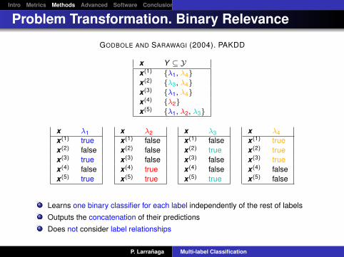
GODBOLE AND SARAWAGI (2004). PAKDD
x Y ⊆ Yx(1) λ1, λ4x(2) λ3, λ4x(3) λ1, λ4x(4) λ2x(5) λ1, λ2, λ3
x λ1 x λ2 x λ3 x λ4x(1) true x(1) false x(1) false x(1) truex(2) false x(2) false x(2) true x(2) truex(3) true x(3) false x(3) false x(3) truex(4) false x(4) true x(4) false x(4) falsex(5) true x(5) true x(5) true x(5) false
Learns one binary classifier for each label independently of the rest of labels
Outputs the concatenation of their predictions
Does not consider label relationships
P. Larranaga Multi-label Classification

Intro Metrics Methods Advanced Software Conclusions
Problem Transformation. Ranking via Single-label Learning
GODBOLE AND SARAWAGI (2004). PAKDD
x Y ⊆ Yx(1) λ1, λ4x(2) λ3, λ4x(3) λ1, λ4x(4) λ2x(5) λ1, λ2, λ3
IGNORE MAX RANDOM MIN COPY-WEIGHT
x(4) λ2 x(1) λ4 x(1) λ1 x(1) λ1 x(1) λ1 0.50x(2) λ4 x(2) λ3 x(2) λ4 x(1) λ4 0.50x(3) λ4 x(3) λ4 x(3) λ1 x(2) λ3 0.50x(4) λ2 x(4) λ2 x(4) λ2 x(2) λ4 0.50x(5) λ1 x(5) λ2 x(5) λ3 x(3) λ1 0.50
x(3) λ4 0.50x(4) λ2 1.00x(5) λ1 0.33x(5) λ2 0.33x(5) λ3 0.33
P. Larranaga Multi-label Classification

Intro Metrics Methods Advanced Software Conclusions
Problem Transformation. Pairwise Methods. Ranking by Pairwise Comparison
HULLERMEIER ET AL. (2008). ARTIFICIAL INTELLIGENCE
x Y ⊆ Yx(1) λ1, λ4x(2) λ3, λ4x(3) λ1, λ4x(4) λ2x(5) λ1, λ2, λ3
λ1-λ2 λ1-λ3 λ1-λ4 λ2-λ3 λ2-λ4 λ3-λ4x(1) true x(1) true x(2) false x(2) false x(1) false x(1) falsex(3) true x(2) false x(5) true x(4) true x(2) false x(3) falsex(4) false x(3) true x(3) false x(5) true
x(4) truex(5) true
It learns d(d − 1)/2 binary models, one for each pair of labels
Each model is trained based on examples that are annotated by at least one ofthe labels, but not bothGiven a new instance, all models are invoked and a ranking is obtained bycounting the votes it receives by each label
λ1 -λ2 λ1-λ3 λ1-λ4 λ2-λ3 λ2-λ4 λ3-λ4x λ1 λ3 λ1 λ3 λ4 λ3
The ranking: rx (λ3) < rx (λ1) < rx (λ4) < rx (λ2)
P. Larranaga Multi-label Classification

Intro Metrics Methods Advanced Software Conclusions
Problem Transformation. Pairwise Methods. Calibrated Label Ranking
HULLERMEIER ET AL. (2008). ARTIFICIAL INTELLIGENCE
λ1-λ0 λ2-λ0 x Y ⊆ Y λ3-λ0 λ4-λ0x(1) true x(1) false x(1) λ1, λ4 x(1) false x(1) truex(2) false x(2) false x(2) λ3, λ4 x(2) true x(2) truex(3) true x(3) false x(3) λ1, λ4 x(3) false x(3) truex(4) false x(4) true x(4) λ2 x(4) false x(4) falsex(5) true x(5) true x(5) λ1, λ2, λ3 x(5) true x(5) false
λ1-λ2 λ1-λ3 λ1-λ4 λ2-λ3 λ2-λ4 λ3-λ4x(1) true x(1) true x(2) false x(2) false x(1) false x(1) falsex(3) true x(2) false x(5) true x(4) true x(2) false x(3) falsex(4) false x(3) true x(3) false x(5) true
x(4) truex(5) true
Extends ranking by pairwise comparison by introducing an additional virtual label(λ0)Pairwise models that include the virtual label correspond to models of binaryrelevance (all examples are used)The final ranking includes the virtual label, used as splitting point betweenpositive and negative labels
λ1 -λ2 λ1-λ3 λ1-λ4 λ2-λ3 λ2-λ4 λ3-λ4 λ1-λ0 λ2-λ0 λ3-λ0 λ4-λ0x λ1 λ3 λ1 λ3 λ4 λ3 λ1 λ0 λ3 λ0
The ranking: rx (λ3) < rx (λ1) < rx (λ0) < rx (λ4) < rx (λ2)⇒ λ3, λ1
P. Larranaga Multi-label Classification

Intro Metrics Methods Advanced Software Conclusions
Problem Transformation. Combining Labels. Label Powerset
BOUTELL ET AL. (2004). PATTERN RECOGNITION
x Y ⊆ Y Labelx(1) λ1, λ4 1001x(2) λ3, λ4 0011x(3) λ1, λ4 1001x(4) λ2 0100x(5) λ1, λ2, λ3 1110
Each different set of labels becomes a different class in a new single-labelclassification taskMost implementations of label powerset classifiers essentially ignore labelcombination that are not presented in the training set (cannot predict unseenlabelsets)Limited training examples for many classes
LabelsetsDataset N d mın(2d ,N) Actualemotions 593 6 64 27medical 978 45 978 94scene 2407 6 64 15yeast 2417 14 2417 198
P. Larranaga Multi-label Classification

Intro Metrics Methods Advanced Software Conclusions
Problem Transformation. Combining Labels. Pruned SetsREAD ET AL. (2008). ICDM
Labelset Countλ1 12λ2 10λ2, λ3 9λ4 7λ3, λ4 2λ1, λ2, λ3 3
Re-introducingpruned examples
Labelset Countλ1 13λ2 11λ2, λ3 10λ4 9
Uses pruning to focus on core combinationsPrunes examples whose labelsets occur fewer times than a user-definedthreshold t (e.g. t = 7)Re-introduces pruned examples along with subsets of their labelsets that doexist more times than
Strategy A: Rank subsets by number of examples and keep the top bStrategy B: Keep all subsets of size greater than gStrategy A (b = 3)λ1 13λ2 11λ2, λ3 10
Strategy B (g = 8)λ1 13λ2 11λ2, λ3 10λ4 9
P. Larranaga Multi-label Classification

Intro Metrics Methods Advanced Software Conclusions
Problem Transformation. Ensemble Methods. Ensembles of Pruned Sets
READ ET AL. (2008). ICDM
Constructs a number of pruned sets by sampling thetraining set (e.g. bootstrap)Some of the pruned examples are partially introduced intothe data by decomposing them into more frequentlyhappening label subsetsGiven a new instance, queries models and averages theirdecisions (each decision concerns all labels): ranking +thresholdingCan form new combination of labelsets
P. Larranaga Multi-label Classification

Intro Metrics Methods Advanced Software Conclusions
Problem Transformation. Ensemble Methods. RAndom k -labELsets (RAkEL)
TSOUMAKAS AND VLAHAVAS (2007). ECML/PKDD
Randomly (without replacement) break a large set of labels into a number (n) ofsubsets of small size (k ), called k -labelsets
For each of them train a multi-label classifier using the label powerset method
Given a new instance, query models and average their decisions per label(thresholding to assign the labelset)
predictionsmodel 3-labelsets λ1 λ2 λ3 λ4 λ5 λ6 λ7 λ8h1 λ1, λ2, λ8 1 0 - - - - - 1h2 λ3, λ4, λ7 - - 0 1 - - 1 -h3 λ2, λ5, λ6 - 1 - - 1 0 - -h4 λ1, λ7, λ8 1 - - - - - 1 0h5 λ3, λ4, λ6 - - 1 1 - 0 - -h6 λ2, λ6, λ8 - 0 - - - 0 - 1
average votes 2/2 1/3 1/2 2/2 1/1 0/3 2/2 2/3prediction (threshold= 0.5) 1 0 1 1 1 0 1 1
P. Larranaga Multi-label Classification

Intro Metrics Methods Advanced Software Conclusions
Problem Transformation. Ensemble Methods. RAndom k -labELsets (RAkEL)
TSOUMAKAS AND VLAHAVAS (2007). ECML/PKDD
BenefitsComputationally simpler sub-problemsMore balanced training setsCan predict unseen labelsets
How to choose n and k?The expected number of votes per label is proportional ton·kd
The larger it is, the higher the effectivenessIt characterizes RAkEL as an ensemble methodk should be small enough to deal with label powersetproblemsn should be large enough to obtain an enough number ofvotes (suggested: k = 3 and n = 2d , expected 6 votes perlabel)
P. Larranaga Multi-label Classification

Intro Metrics Methods Advanced Software Conclusions
Problem Transformation. Ensemble Methods. RAndom k -labELsets (RAkEL)
ROKACH AND ITACH (2010). ICML, WORKSHOP ML
Y axis: coverage probability of all pairs of labels. X axis: number of k labelsets (Rokach and Itach, 2010)
RAkEL no guarantees to cover all subsets of labels at size r < kMinimum required subsets of labels at size k that cover all the possible subsetsof labels at size r (r < k )Improve RAkEL by constructing an ensemble of label powerset classifiers basedon meaningful subsets rather than random subsetsThe subsets are selected in advance providing higher and stabler predictiveperformance
P. Larranaga Multi-label Classification

Intro Metrics Methods Advanced Software Conclusions
Problem Transformation. Ensemble Methods. RAndom k -labELsets (RAkEL)
ITACH ET AL. (2009). ECML/PKDD, WORKSHOP ML
Analogy between the labelset selection method and the transportation model
Transportation model: type of network problem used for planning how to shipcommodities from a source (factory) to a destination (warehouses) at minimumcost
ROKACH AND ITACH (2010). ICML, WORKSHOP ML
Formulation of the k -labelset matrix design problem (ensuring coverage at sizer ) equivalent to the set covering problem
For a given number of labels, d , and a given source-subset labels, k , the numberof labelsets, n, required to cover all label pairs is:
2k(k − 1)
(d2 ) ≤ n ≤
dk
+ (d2 )−
d(k − 1)
2
d = 8; k = 3⇒ 10 ≤ n ≤ 23
P. Larranaga Multi-label Classification

Intro Metrics Methods Advanced Software Conclusions
P.T. Identifying Label Dependencies. Correlation-based Pruning of Stacked BR Models
TSOUMAKAS ET AL. (2009). ECML WORKSHOP ML
2BR: stacking of BR classifiers (BR is used in two consecutive levels)Alleviate the label correlations problem by identifying them explicitly using φcorrelationPrune models participating in the stacking process by thresholding the degree oflabel correlationFirst level BR: (for i = 1, ..., d)
hi : ΩX1 × · · · × ΩXm → λi
(x1, ..., xm) 7→ λhii
Second level BR: (for i = 1, ..., d)
h2i : Hi = Φ(λ
h11 × · · · × λ
hdd ) ⊆ λh1
1 × · · · × λhdd → λi
λj ¬λj
λi a b φ(λi , λj ) = |a·d−b·c|√(a+b)(c+d)(a+c)(b+d)
¬λj c d
Hi = ⊗λhjj ||φ(λi , λj )| > t
P. Larranaga Multi-label Classification

Intro Metrics Methods Advanced Software Conclusions
P.T. Identifying Label Dependencies. Chi-Dep
TENENBOIM ET AL. (2010). ICML WORKSHOP ML
LPBRA model allowing to balance between BR and LP by modeling existingdependencies between labels
LPBR algorithmStep 1. Start from total independence (BR model)Step 2. Cluster the pair of most dependent labels (chi-square test)Step 3. Build and evaluate the new modelStep 4. Compare accuracy to the previous model. If improved, accept thenew modelRepeat Steps 2-4 until stopping condition is metReturn the latest accepted model
Stopping condition:Number of allowed “non-improvement” label pairs is exceededChi-square value is below thresholdNo more pairs to considerAll labels are in the same cluster
P. Larranaga Multi-label Classification

Intro Metrics Methods Advanced Software Conclusions
P.T. Identifying Label Dependencies. Chi-Dep Ensemble
TENENBOIM ET AL. (2010). ICML WORKSHOP ML
Ensemble of Chi-Dep classifiers1 Randomly generate a number (e.g. 10,0000) of label set
partitions2 Compute a score for each partition
Partition score:∑χ2∗λi ,λj−∑χ2∗λq ,λr
where λi , λj belong tothe same group and λq , λr are in different groupsχ2∗λi ,λj
= χ2λi ,λj− χ2
critical corresponds to a normalization ofthe chi-square value
3 Select the M high-scored partitions as members of theensemble
4 Classification step:- Collect classifications from all models;- Compute averaged score for each label;- Return positive labels (score above the
threshold)P. Larranaga Multi-label Classification

Intro Metrics Methods Advanced Software Conclusions
P.T. Identifying Label Dependencies. Hierarchy of Multi-label Classifiers
TSOUMAKAS ET AL. (2008). ECML/PKDD2008 WORKSHOP ON MMD’08
Hierarchy Of Multi-label classifiERs (HOMER)
HOMER constructs a hierarchy of multi-label classifiers each one dealing with amuch smaller set of labels and a more balanced example distributionBalanced k -means: approximately equal number of labels in each cluster
P. Larranaga Multi-label Classification

Intro Metrics Methods Advanced Software Conclusions
Adaptation Methods
BoostingRank-SVMDecision TreeNeural NetworkK -Nearest NeighborInstance Based Using Mallows ModelInstance Based + Logistic RegressionGenerative Parametric Mixture ModelProbabilistic Chain ClassifierBayesian Network
P. Larranaga Multi-label Classification

Intro Metrics Methods Advanced Software Conclusions
Adaptation Methods. Boosting
SCHAPIRE AND SINGER (2000). MACHINE LEARNING
Map the original multi-label learning problem into a binarylearning problem, which is solved by the traditionalAdaBoost algorithmTransform each multi-label training example (x (i),Y i)(1 ≤ i ≤ N) into d binary single labeled examples,((x (i), y),Y i(y)) for all y ∈ Y where (x (i), y) denotes theconcatenation of x (i) and label y , and Y i(y) = +1 if y ∈ Y i
and −1 otherwiseClassical AdaBoost is employed to learn from thetransformed binary-labeled examples iteratively withone-level decision trees as base learners
P. Larranaga Multi-label Classification

Intro Metrics Methods Advanced Software Conclusions
Adaptation Methods. Rank-SVMELISSEEFF AND WESTON (2002). NIPS
A maximum margin approach for multi-label learning,implemented with kernel trick to incorporate non-linearityAssume one classifier for each individual label, and definemulti-label margin on the whole training set, which is thenminimized under quadratic programming frameworkClassification system: d linear classifiers,gk (x)|1 ≤ k ≤ d) each with weight wk and bias bk :
gk (x) = wTk · x + bk
Margin definition:For an example (x (i),Y i ): min
(k,l)∈Y i×Y iw T
k ·x+bk−w Tl ·x−bl
||w k−w l ||For the training set S:min(x (i),Y i )∈Smin
(k,l)∈Y i×Y iw T
k ·x+bk−w Tl ·x−bl
||w k−w l ||Optimization under quadratic programming framework inits dual form with incorporation of kernel trick
P. Larranaga Multi-label Classification

Intro Metrics Methods Advanced Software Conclusions
Adaptation Methods. Decision Tree
CLARE AND KING (2001). PKDD
Multi-label C4.5: an extension of the popular C4.5 decisiontree algorithm to deal with multi-label dataBased on the definition of multi-label entropy:
Given a set of multi-label examplesD = (x (1),Y(1)), ..., (x (N),Y(N))Let P(y) denote the probability that an example in D haslabel yMLH(Y) =
∑y∈Y H(y)
=∑
y∈Y P(y) log(P(y)) + (1− P(y)) log(1− P(y))The previous formula assumes independency between thelabels
The decision tree is constructed recursively in the sameway of C4.5 using information gain as splitting criterion forselecting attributes in the tree
P. Larranaga Multi-label Classification

Intro Metrics Methods Advanced Software Conclusions
Adaptation Methods. Neural Network
ZHANG AND ZHOU (2006). IEEE TRANSACTIONS ON KNOWLEDGE AND DATAENGINEERING
BP-MLL: an extension of the popular back propagation algorithm for learningneural networks to deal with multi-label data
Error function capturing the characteristics of multi-label learning, i.e. labelsbelonging to an example should be ranked lower than those not belonging to thatexample
E =N∑
i=1
Ei =N∑
i=1
1
|Yi ||Y i |
∑(k,l)∈Yi×Y i
exp(−(oil − oi
k ))
where oij denotes the output on x(i) on the j-th label
Network architecture: a) single-hidden-layer forward neural networks; b) adjacentlayers fully connected; c) each input corresponds to a dimension of the inputspace; d) each output corresponds to an individual label
Parameter optimization: gradient descent + error back-propagation
P. Larranaga Multi-label Classification

Intro Metrics Methods Advanced Software Conclusions
Adaptation Methods. K -Nearest Neighbor
ZHANG AND ZHOU (2007). PATTERN RECOGNITION
Multi-label k -NN (ML-kNN) is a binary relevance learner, i.e., it learns a singleclassifier hi for each label λi ∈ YThe single-label classifier, hi , is implemented as a combination of k -NN andBayesian inference (MAP principle)
For a new instance x to be classified1 Identify its k nearest neighbors in the training set, Nk (x)2 Compute its d-dimensional membership counting vector:
cNk (x) = (c1,x , ..., cd,x ), where cl,x counts the number of examples inNk (x) having the l-th label
3 Noticing that P(λl ∈ Y x |cl,x ) ∝ P(cl,x |λl ∈ Y x ) · P(λl ∈ Y x ), thedecision rule for the i-th single-label classifier is:
hi (x) =
1 if P(ci,x |λi ∈ Yx ) · P(λi ∈ Yx ) ≥ P(ci,x |λi 6∈ Y x ) · P(λi 6∈ Y x )
0 otherwise
The probabilities above are estimated from the training dataset
P. Larranaga Multi-label Classification

Intro Metrics Methods Advanced Software Conclusions
Adaptation Methods. Instance Based Using Mallows Model
CHENG AND HULLERMEIER (2009). ECML WORKSHOP MLD
Label ranking richer than multi-label: λπ−1x (1)
≺x · · · ≺x λπ−dx (1)
Distance between two rankings counting the number of discordant label pairs
D(π, σ) = #(i, j)| π(i) > π(j), σ(i) < σ(j)
Calibrated label ranking: introduce a virtual (neutral) label λ0, such that ifλi ≺x λ0 then λi is selectedMallows probability distribution for permutations:
P(σ|θ, π) =exp(−θD(π, σ))
φ(θ, π)
where π is the spread parameter, and θ > 0 is the location parameter. The modeis at σ = π and when θ = 0 the Mallows probability distribution is uniformGiven a new instance, x , and its k neighbors, x(1), ..., x(k), with associatedlabels, Y (1), ...,Y (k), assuming an underlying (calibrated) label ranking and theMallows model:
P(E(Y (i)x )|θ, π) =
∑σ∈E(Y (i)
x )
P(σ|θ, π)
where E(Y (i)x ) denotes the set of label rankings consistent with Y (i)
x
P. Larranaga Multi-label Classification

Intro Metrics Methods Advanced Software Conclusions
Adaptation Methods. Instance Based Using Mallows Model
CHENG AND HULLERMEIER (2009). ECML WORKSHOP MLD
Instance based prediction of the label ranking posed as a maximum likelihoodproblem
The likelihood of the neighborhood of x is given by:
L(Y (1)x , ...,Y (k)
x |θ, π) =k∏
i=1
P(E(Y (i)x )|θ, π) =
k∏i=1
∑σ∈E(Y (i)
x )
exp(−θD(π, σ))
φ(θ, π)
Finding the maximum likelihood estimation of π and θ is for Mallows distributionextremely difficult, but .... in the context of multi-label classification it can beshown that
the optimal multi-label prediction can simply be found by sorting the labelsaccording to their frequency of occurrence in the neighborhood, breakingties with the label frequency in the complete training data
P. Larranaga Multi-label Classification

Intro Metrics Methods Advanced Software Conclusions
Adaptation Methods. Instance Based + Logistic Regression
CHENG AND HULLERMEIER (2009). MACHINE LEARNING
Instance based embedded into logistic regression (single-label)
k -NN: y0 = arg maxy #x(i) ∈ Nk (x0)|y (i) = yIB(k -NN) as LR: consider the labels of neighbored instances as “features” of thequery x0 whose label is to be estimated
Let’s define: p0 = p(y0 = +1); π0 = p(y0 = +1|y (i)); δi = d(x0, x(i))
We obtain: π01−π0
=p(y(i)|y0=+1)
p(y(i)|y0=−1)· p0
1−p0= ρ · p0
1−p0
Defining: ρ = exp(y (i) · αδi
), and ln po1−po
= w0, we have: ln π01−π0
= w0 + α · y(i)
δi
Taking the complete neighborhood Nk (x0):
ln π01−π0
= w0 + α ·∑
x i∈Nk (x0)y(i)
δi= w0 + α · w+(x0)
The posterior probability π0 of the query x0 is (IBLR): π0 =exp(w0+α·w+(x0))
1+exp(w0+α·w+(x0))
Including additional features (IBLR+):ln π0
1−π0= w0 + α · w+(x0) +
∑ϕs∈F βsϕs(x0) with F ⊆ φ1, ..., φm
P. Larranaga Multi-label Classification

Intro Metrics Methods Advanced Software Conclusions
Adaptation Methods. Instance Based + Logistic Regression
CHENG AND HULLERMEIER (2009). MACHINE LEARNING
Extension to multi-label classification (IBLR-ML and IBLR-ML+)
Train a classifier hi for each label λi with i = 1, ..., d
lnπ
(i)0
1−π(i)0
= w (i)0 +
∑dj=1 α
(i)j · w
(i)+j (x0)
where π(i)0 denotes the (posterior) probability that λi is relevant for x0, and
w (i)+j (x0) =
∑x∈Nk (x0) κ(x0, x) · yj (x) is a summary of the presence of the j-th
label λj in the neighborhood of x0; here yj (x) = +1 if λj is present for theneighbor x , and yj (x) = −1 in case it is absent
This approach is able to take interdependencies between classes intoconsideration, because α(i)
j indicates to what extent the relevance of label λi isinfluenced by the relevance of λj
Taking additional features into account:
lnπ
(i)0
1−π(i)0
= w (i)0 +
∑dj=1 α
(i)j · w
(i)+j (x0) +
∑ϕs∈F β
(i)s ϕs(x0)
P. Larranaga Multi-label Classification

Intro Metrics Methods Advanced Software Conclusions
Adaptation Methods. Generative Parametric Mixture Model
MCCALLUM (1999) IN AAAI WORKSHOP ON TEXT LEARNING, AND UEDA AND SAITO(2003) IN NIPS
The word distribution given a set of labels is determined by a mixture of worddistributions, one for each single labelWord vocabulary: w = (w1, ...,wm)
P(w |λi ) word distribution given a single label λi ∈ YP(w |Y ) word distribution given a set of labels Y ⊆ YGiven a test document x , its associated label set Y∗ is determined as:
Y∗ = arg maxY⊆YP(Y |x) = arg maxY⊆YP(Y )P(x |Y )
= arg maxY⊆YP(Y )∏
w∈xP(w |Y )
= arg maxY⊆YP(Y )∏
w∈x
∑λj∈Y
γYλi
P(w |y)
The terms P(Y ), and P(w |y) are estimated from the training set by frequencycountingThe parameters γY
λi(with Y ⊆ Y) are learned by an EM-style procedure
P. Larranaga Multi-label Classification

Intro Metrics Methods Advanced Software Conclusions
Adaptation Methods. Probabilistic Chain Classifier
DEMBCZYnSKI ET AL. (2010). ICML
Overcoming the label independence assumption of thebinary relevance methodLearn d functions hi on augmented input spacesΩX ×0,1
i−1, respectively, taking c1, ..., ci−1 as additionalfeatures:
hi : ΩX × 0,1i−1 → [0,1]
(x , c1, ..., ci−1) 7→ p(ci |x , c1, ..., ci−1)
Classifier chain was first introduced in multi-labelclassification by READ ET AL. (2009) in ECML/PKDDalbeit without a probabilistic interpretation
P. Larranaga Multi-label Classification

Intro Metrics Methods Advanced Software Conclusions
Adaptation Methods. Bayesian NetworkMULTIPLE DIAGNOSIS PROBLEM
X1 . . . Xm C1 . . . Cd
(x (1), c(1)) x (1)1 . . . x (1)
m c(1)1 . . . c(1)
d(x (2), c(2)) x (2)
1 . . . x (2)m c(2)
1 . . . c(2)d
. . . . . . . . .
(x (N), c(N)) x (N)1 . . . x (N)
m c(N)1 . . . c(N)
d
Optimal diagnosis as abductive inference (MPE)
(c∗1 , . . . , c∗d ) = arg max(c1,...,cd )p(C1 = c1, . . . ,Cd = cd |X1 = x1, . . . ,Xm = xm)
= arg max(c1,...,cd )p(C1 = c1, . . . ,Cd = cd )p(X1 = x1, . . . , Xm = xm|C1 = c1, . . . ,Cd = cd )
Number of parameters to be estimated: 2d − 1 + 2d (2m − 1)
d m number parameters3 10 ' 8 · 103
5 20 ' 33 · 106
10 50 ' 11 · 1017
P. Larranaga Multi-label Classification

Intro Metrics Methods Advanced Software Conclusions
Adaptation Methods. Bayesian Network
MULTI-DIMENSIONAL BAYESIAN NETWORK CLASSIFIER (MBC)
The set of vertices V is partitioned into:VC = C1, ...,Cd of class variables andVX = X1, ...,Xm of feature variables, with (d + m = n)
P. Larranaga Multi-label Classification

Intro Metrics Methods Advanced Software Conclusions
Adaptation Methods. Bayesian NetworkMULTI-DIMENSIONAL BAYESIAN NETWORK CLASSIFIER (MBC)
(a) Empty-empty MBC
(b) Tree-tree MBC
(c) Polytree-DAG MBC
P. Larranaga Multi-label Classification

Intro Metrics Methods Advanced Software Conclusions
Adaptation Methods. Bayesian NetworkZHANG ET AL. (2009). INFORMATION SCIENCES: AN INTERNATIONAL
JOURNAL
MLNB: Multi-Label Naive Bayes ≡ Empty-empty MBCA two-stage filter-wrapper feature selection strategy isincorporated:
First stage (filter): feature extraction techniques based onprinciple component analysis (PCA)Second stage (wrapper): subset selection techniquesbased on a genetic algorithm (GA) (on the space of PCAs)are used to choose the most appropriate subset of featuresfor classification
The correlations between different labels are explicitlyaddressed by the GA fitness function: a linear combinationbetween Hamming loss and ranking lossGaussian assumption: the density of the features variablesgiven the class values follows a Gaussian density
P. Larranaga Multi-label Classification

Intro Metrics Methods Advanced Software Conclusions
Adaptation Methods. Bayesian NetworkVAN DER GAAG AND DE WAAL. (2006). PGM
Tree-tree MBC learned in three steps:The class subgraph is learnt by searching for the maximumweighted undirected spanning tree and transforming it intoa directed tree using Chow and Liu’s (1968) algorithm
The weight of an edge is the mutual information between apair of class variables
For a fixed bridge subgraph, the feature subgraph is thenlearnt by building a maximum weighted directed spanningtree (Chu and Liu, 1968)
The weight of an arc is the conditional mutual informationbetween pairs of feature variables given the parents(classes) of the second feature determined by the bridgesubgraph
The bridge subgraph is greedily changed in a wrapper-likeway trying to improve the considered metric (0/1 subsetaccuracy)
P. Larranaga Multi-label Classification

Intro Metrics Methods Advanced Software Conclusions
Adaptation Methods. Bayesian Network
DE WAAL AND VAN DER GAAG (2007). ECSQARU
Theoretical work on Polytree-polytree MBC:The algorithms for learning the polytrees for the class andfeature subgraphs separately are based on Rebane andPearl’s (1987) algorithmFor the feature subgraph the algorithm requiresconsidering all the class variables in the conditional mutualinformation (unfeasible in real applications)It omits how to find the bridge subgraph
P. Larranaga Multi-label Classification

Intro Metrics Methods Advanced Software Conclusions
Adaptation Methods. Bayesian Network
RODRIGUEZ AND LOZANO (2008). HAIS
K-DB-K-DB MBC:K -DB: K -dependence Bayesian network structure allowseach variable to have at most K parentsEach permitted structure is coded as an individual in agenetic algorithm with three substrings, one per subgraphThe objective function is a vector of d components, each ofthem representing the accuracy in each class variableNSGA-II (Deb et al, 2000) chosen as the multi-objectivegenetic algorithm to find non-dominated structures
P. Larranaga Multi-label Classification

Intro Metrics Methods Advanced Software Conclusions
Adaptation Methods. Bayesian Network
BIELZA ET AL. (2010). UPM-DIA TECHNICAL REPORT
Filter approach to DAG-DAG MBC: Class + alternating bridgeand feature
P. Larranaga Multi-label Classification

Intro Metrics Methods Advanced Software Conclusions
Adaptation Methods. Bayesian Network
BIELZA ET AL. (2010). UPM-DIA TECHNICAL REPORT
Filter approach to DAG-DAG MBC: Class + alternating bridgeand feature
P. Larranaga Multi-label Classification

Intro Metrics Methods Advanced Software Conclusions
Adaptation Methods. Bayesian Network
BIELZA ET AL. (2010). UPM-DIA TECHNICAL REPORT
Filter approach to DAG-DAG MBC: Class + alternating bridgeand feature
P. Larranaga Multi-label Classification

Intro Metrics Methods Advanced Software Conclusions
Adaptation Methods. Bayesian Network
BIELZA ET AL. (2010). UPM-DIA TECHNICAL REPORT
Filter approach to DAG-DAG MBC: Class + alternating bridgeand feature
P. Larranaga Multi-label Classification

Intro Metrics Methods Advanced Software Conclusions
Adaptation Methods. Bayesian Network
BIELZA ET AL. (2010). UPM-DIA TECHNICAL REPORT
Filter approach to DAG-DAG MBC: Class + alternating bridgeand feature
P. Larranaga Multi-label Classification

Intro Metrics Methods Advanced Software Conclusions
Adaptation Methods. Bayesian Network
BIELZA ET AL. (2010). UPM-DIA TECHNICAL REPORT
Filter approach to DAG-DAG MBC: Class + alternating bridgeand feature
P. Larranaga Multi-label Classification

Intro Metrics Methods Advanced Software Conclusions
Adaptation Methods. Bayesian Network
BIELZA ET AL. (2010). UPM-DIA TECHNICAL REPORT
Filter approach to DAG-DAG MBC: Class + alternating bridgeand feature
P. Larranaga Multi-label Classification

Intro Metrics Methods Advanced Software Conclusions
Adaptation Methods. Bayesian Network
BIELZA ET AL. (2010). UPM-DIA TECHNICAL REPORT
Filter approach to DAG-DAG MBC: Class + alternating bridgeand feature
P. Larranaga Multi-label Classification

Intro Metrics Methods Advanced Software Conclusions
Adaptation Methods. Bayesian Network
BIELZA ET AL. (2010). UPM-DIA TECHNICAL REPORT
Wrapper approach to DAG-DAG MBC
i = 01. G(i) = ∅. Acc = Acc(i)
2. Whenever there are arcs that can be added to G(i) (and not previously discarded):Add one arc to GC (i), GCX (i) or GX (i) and obtain the new G(i+1) and Acc(i+1)
3. If Acc(i+1) > Acc(i), Acc = Acc(i+1), i = i + 1, and go to 2Else discard the arc and go to 2
4. Stop and return G(i) and Acc
P. Larranaga Multi-label Classification

Intro Metrics Methods Advanced Software Conclusions
Adaptation Methods. Bayesian NetworkBORCHANI ET AL. (2010). PGM
(a) A CB-decomposable MBC
(b) Its two maximal connected components
MBC is class-bridge decomposable or (CB-decomposable) if:
1 GC ∪ GCX can be decomposed as: GC ∪ GCX =⋃r
i=1(GC i ∪ G(CX ) i) where
GC i ∪ G(CX ) iwith i = 1, ..., r are its maximal connected components
2 Non-shared children: Ch(VC i ) ∩ Ch(VC j ) = ∅, with i, j = 1, ..., r and i 6= j , whereCh(VC i ) denotes the children of all the variables in VC i
P. Larranaga Multi-label Classification

Intro Metrics Methods Advanced Software Conclusions
Adaptation Methods. Bayesian NetworkBORCHANI ET AL. (2010). PGM
MBC CB-decomposable for alleviating the MPE computations
(a) A CB-decomposable MBC
(b) Its two maximal connected components
maxc1,...,c5 p(C1 = c1, ...,C5 = c5|X1 = x1, ..., X6 = x6) ∝maxcp(c1)p(c2)p(c3|c2)p(c4)p(c5|c4)p(x1|c1)p(x2|c1, c2, x1)p(x3|c3)p(x4|c3, x3, x5, x6)p(x5|c4, c5, x6)p(x6|c5)= maxc1,c2,c3 p(c1)p(c2)p(c3|c2)p(x1|c1)p(x2|c1, c2, x1)p(x3|c3)p(x4|c3, x3, x5, x6)·
maxc4,c5 p(c4)p(c5|c4)p(x5|c4, c5, x6)p(x6|c5)
Here VC1 = C1,C2,C3,VC2 = C4,C5,Ch(VC1) = X1, X2, X3, X4 and Ch(VC2) = X5, X6. Note
that Ch(VC1) ∩ Ch(VC2) = ∅ as required in the definition
P. Larranaga Multi-label Classification

Intro Metrics Methods Advanced Software Conclusions
Adaptation Methods. Bayesian NetworkBORCHANI ET AL. (2010). PGM
Learning CB decomposable MBCs. Phase I. Learn bridge subgraph
X2
C1
X5 X1
C2
X4X2 X1X4
C3
X3X6 X5
C4
X4X6
Starting from an empty graphical structure, learn a selective naive Bayes for each class variable
X2
C1
X1
C2
X3
C3
X6X4 X5
C4
Check the non-shared children property to induce an initial CB-decomposable MBC (remove all commonchildren based on two criteria: feature insertion rank and accuracy)The result of this phase is a simple CB-decomposable MBC where only the bridge subgraph is defined(class and feature subgraphs are empty)
P. Larranaga Multi-label Classification

Intro Metrics Methods Advanced Software Conclusions
Adaptation Methods. Bayesian Network
BORCHANI ET AL. (2010). PGM
Learning CB decomposable MBCs. Phase II. Learn feature subgraph
X2
C1
X1
C2
X3
C3
X6X4 X5
C4
Introduce the dependence relationships between the feature subgraph
Fix the maximum number of iterations
In each iteration an arc is selected at random between a pair of feature variables. If there is an accuracyimprovement, the arc is added, otherwise it is discarded
P. Larranaga Multi-label Classification

Intro Metrics Methods Advanced Software Conclusions
Adaptation Methods. Bayesian NetworkBORCHANI ET AL. (2010). PGM
Learning CB decomposable MBCs. Phase III. Merge maximal connected components
X2
C1
X1
C2
X3
C3
X6X4 X5
C4
X2
C1
X1
C2
X3
C3
X6X4 X5
C4
Merging the maximal connected components Bridge subgraph update
All possible arc additions between the class variables are evaluated, adding the arc improving the accuracythe most (from r to r − 1 maximal connected components)A bridge update step is performed inside the new induced maximal connected component
X2
C1
X1
C2
X3
C3
X6X4 X5
C4
Feature subgraph update
Update the feature subgraph by inserting, one by one, additional arcs between feature variablesThis phase iterates over these three steps (stopping criteria: no more component merging can improve theaccuracy or r = 1)
P. Larranaga Multi-label Classification

Intro Metrics Methods Advanced Software Conclusions
Outline
1 Introduction
2 Evaluation Metrics
3 Methods for Learning Multi-label Classifiers
4 Advanced Topics
5 Software
6 Conclusions
P. Larranaga Multi-label Classification

Intro Metrics Methods Advanced Software Conclusions
Structured Predicted OutputsBAKIR ET AL. (2007). PREDICTING STRUCTURED DATA. MIT PRESS
PARKER ET AL. (2009). STRUCTURED PREDICTION. SPECIAL ISSUE. MACHINELEARNING
Structured prediction (or structured classification) is thetask of predicting a collection of related variables givensome inputThere is some information about the relationships betweenthe variables to be predicted (e.g. hierarchical: a treestructure)
P. Larranaga Multi-label Classification

Intro Metrics Methods Advanced Software Conclusions
Multi-instance Multi-labelZHANG AND ZHOU (2008). ICDM; ZHA ET AL. (2008). CVPR; JIN ET AL. (2009).
CVPR
Traditional supervised classification Multi-label classification
Multi-instance classification Multi-instance multi-label classification
P. Larranaga Multi-label Classification

Intro Metrics Methods Advanced Software Conclusions
Multi-label Classification in Parallel TasksLOZA (2010). ICML. WORKSHOP MLD’10
Book scenario: the same book classified according to different criteriaCriteria:
Genres: crime, mystery, thrillerSubjects: private investigators, Orient Express, train, IstanbulAdaptations: book, video game, movie, theaterLanguage: English, Spanish, German, French, Italian, Chinese
Each criteria (a multi-label problem) treated separately or jointly (exploitinginter-criteria relations in addition to intra-criteria relations)EUR-LEX (http://www.ke.tu-darmstadt.de/resources/eurlex):19,348 documents for European Union organized into 3 different criteria: subjectmatter (201 labels), directory code (410 labels), EUROVOC (3,956 labels)
P. Larranaga Multi-label Classification

Intro Metrics Methods Advanced Software Conclusions
Graded Multi-label ClassificationCHENG ET AL. (2010). ICML
Vertical reduction Horizontal reduction
Replace simple yes or no labels by membership degrees taken from a finiteordered scale such as:M = not at all, somewhat, almost, fullyClass membership in the sense of fuzzy set theoryVertical reduction: prediction of membership degree (ordinate) for each labelHorizontal reduction: prediction of a subset of labels (indicated by black circles)on each levelData set BeLa-E from social psychology: 50 variables (sex, age + 48 gradeddegree of importance of different properties of the future job evaluated on anordinal scale). Features and classes randomly selected
P. Larranaga Multi-label Classification

Intro Metrics Methods Advanced Software Conclusions
Multi-label Semi-supervised LearningORTIGOSA-HERNANDEZ ET AL. (2010). TAMIDA
X1 X2 . . . Xm C1 C2 . . . Cd
x (1)1 x (1)
2 . . . x (1)m c(1)
1 c(1)2 . . . c(1)
dx (2)
1 x (2)2 . . . x (2)
m c(2)1 c(2)
2 . . . c(2)d
. . . . . . . . . . . . . . . . . . . . . . . .
x (L)1 x (L)
2 . . . x (L)m c(L)
1 c(L)2 . . . c(L)
dx (L+1)
1 x (L+1)2 . . . x (L+1)
m ? ? . . . ?x (L+2)
1 x (L+2)2 . . . x (L+2)
m ? ? . . . ?. . . . . . . . . . . . . . . . . . . . . . . .
x (N)1 x (N)
2 . . . x (N)m ? ? . . . ?
The structural EM algorithm (Friedman (1998). UAI)Learn an initial model
Repeat until convergence the following two steps:1 Expectation step: Using the current model, impute the missing data with its
expected values2 Maximization step: Using the expectation of the missing data as real data,
learn the model (structure and parameters) that maximizes the marginallikelihood
P. Larranaga Multi-label Classification

Intro Metrics Methods Advanced Software Conclusions
Multi-label with Missing in Blocks in the Classes
X1 . . . Xm C1 C2 C3 C4
x (1)1 ... x (1)
m c(1)1 ? ? c(1)
4... ... ... ... ? ? ...x (N1)
1 ... x (N1)m c(N1)
1 ? ? c(N1)4
x (N1+1)1 ... x (N1+1)
m c(N1+1)1 c(N1+1)
2 ? ?... ... ... ... ... ? ?x (N1+N2)
1 ... x (N1+N2)m c(N1+N2)
1 c(N1+N2)2 ? ?
... ... ... ... ... ... ...
... ... ... ... ... ... ...
... ... ... ... ... ... ...
x(∑r−1
i=1 Ni +1)
1 ... x(∑r−1
i=1 Ni +1)m ? ? c
(∑r−1
i=1 Ni +1)
3 c(∑r−1
i=1 Ni +1)
4... ... ... ? ? ... ...x (N)
1 ... x (N)m ? ? c(N)
3 c(N)4
P. Larranaga Multi-label Classification

Intro Metrics Methods Advanced Software Conclusions
Multi-label Data StreamsReal word problems: news, forums, e-mail, socialnetworking sites, scene and video classification,....Generalize definitions of different types of concept drifts:P(x1, ..., xm), P(cj |x1, ..., xm),P(ci , cj |x1, ..., xm), ..., P(ci),P(ci , cj), ..., P(c1, ..., cd )
Design methods for detecting differences statisticallysignificant between Pt (·|·) and Pt+1(·|·)Adapt:
multi-label classification methods to the data streamconceptdata stream methods to multi-label context
Some works:Qu et al. (2009) ACMLRead et al. (2009) ECML; Read et al. (2010) TechnicalReport, University of Waikatohttp://sourceforge.net/projects/moa-datastream/
P. Larranaga Multi-label Classification

Intro Metrics Methods Advanced Software Conclusions
Multiple Stratified k -Fold Cross-validation
The problem
Given D = (x(1), c(1)), ..., (x(N), c(N)) with x(j) = (x (j)1 , ..., x (j)
m ) and
c(j) = (c(j)1 , ..., c(j)
d )
(i) D =⋃k
i=1 Di and(ii) D i ⋂ D j = ∅ for all i, j = 1, .., k with i 6= jthat is optimal with respect to the Kullback-Leibler divergence of theempirical distribution of the d-dimensional variable C = (C1, ...,Cd ):
mink∑
i=1
DK−L(pD(c1, ..., cd ); pDi (c1, ..., cd ))
Evolutionary computation based approach
An individual represents a possible partitionAn individual is encoded by an N length array with values taken from theset 1, ..., kEach value is taken at least bN
k c timesFitness function to be minimized:∑k
i=1 DK−L(pD(c1, ..., cd ); pDi (c1, ..., cd ))
P. Larranaga Multi-label Classification

Intro Metrics Methods Advanced Software Conclusions
Searching for the Predictor Features and the Labels
Disease gene association: identifying which DNA variations are highlyassociated with a specific diseaseSingle nucleotide polymorphisms (SNPs) as the most common form of DNAvariation
Haplotypes as sets of SNPs localized on one chromosome
Haplotype tagging SNP (htSNP) selection, Lee and Shatkay (2006): Find asubset of SNPs on a haplotype (with a size smaller than some pre-specifiedconstant) that can predict the remaining unselected ones
Angiotensin converting enzyme (ACE): 78 SNPs on chromosome 17q23Human lipoprotein lipase (LPL): 88 SNPs on chromosome 19q13,22Inflamatory bowel disease (IBD5): 103 SNPS on chromosome 5q31
P. Larranaga Multi-label Classification

Intro Metrics Methods Advanced Software Conclusions
Outline
1 Introduction
2 Evaluation Metrics
3 Methods for Learning Multi-label Classifiers
4 Advanced Topics
5 Software
6 Conclusions
P. Larranaga Multi-label Classification

Intro Metrics Methods Advanced Software Conclusions
Software
Mulan a open-source software in Weka athttp://mulan.sourceforge.net contains:
Methods: binary relevance, calibrated label ranking, labelpowerset, multi-label stacking, RAkEL, HOMER, HMC,ML-kNN, BRkNN, IBLR, BPMLLMetrics: 0/1 subset accuracy, accuracy, Hamming loss,precision, recall, F-measure, macro, micro
Matlab code athttp://lamda.nju.edu.cn/datacode/MLkNN.htmcontains: MLK NN, BPMLLMeka library athttp://www.cs.waikato.ac/nz/vjmr30/#softwarecontains: pruned sets, classifier chains
P. Larranaga Multi-label Classification

Intro Metrics Methods Advanced Software Conclusions
Outline
1 Introduction
2 Evaluation Metrics
3 Methods for Learning Multi-label Classifiers
4 Advanced Topics
5 Software
6 Conclusions
P. Larranaga Multi-label Classification

Intro Metrics Methods Advanced Software Conclusions
MULTI-LABEL CLASSIFICATION
Hot topic in machine learningPossibility of generalize standard methods and evaluationproceduresChallenging real word problems
P. Larranaga Multi-label Classification

Intro Metrics Methods Advanced Software Conclusions
Many Thanks to
1 ColleaguesA. BahamondeL. BaumelaC. BielzaH. BorchaniJ. D. RodrıguezG. LiJ. Ortigosa-HernandezS. Ventura
2 ProjectsCajal Blue Brain (Spanish Ministry of Science andInnovation)Consolider Ingenio 2010-CSD2007-00018Dynamo (Foncicyt, European Union and Mexico)TIN2008-06815-C02-02, TIN2010-20900-C04-04
P. Larranaga Multi-label Classification

Intro Metrics Methods Advanced Software Conclusions
MULTI-LABEL CLASSIFICATION
Pedro Larranaga
Computational Intelligence GroupArtificial Intelligence Department
Technical University of Madrid
V Simposio de Teorıa y Aplicaciones de Minerıa de Datos. TAMIDA’2010Valencia, September 9, 2010
P. Larranaga Multi-label Classification