General rights Copyright and moral rights for the publications made accessible in the public portal are retained by the authors and/or other copyright owners and it is a condition of accessing publications that users recognise and abide by the legal requirements associated with these rights.

• Users may download and print one copy of any publication from the public portal for the purpose of private study or research. • You may not further distribute the material or use it for any profit-making activity or commercial gain • You may freely distribute the URL identifying the publication in the public portal

If you believe that this document breaches copyright please contact us providing details, and we will remove access to the work immediately and investigate your claim.

Downloaded from orbit.dtu.dk on: Jun 24, 2018

Multi-material topology optimization of laminated composite beams witheigenfrequency constraints

Blasques, José Pedro Albergaria Amaral

Published in:Composite Structures

Link to article, DOI:10.1016/j.compstruct.2013.12.021

Publication date:2014

Link back to DTU Orbit

Citation (APA):Blasques, J. P. A. A. (2014). Multi-material topology optimization of laminated composite beams witheigenfrequency constraints. Composite Structures, 111, 45-55. DOI: 10.1016/j.compstruct.2013.12.021

Multi-material topology optimization of laminated composite beams with eigenfrequencyconstraints

Jose Pedro Blasques∗

Department of Wind Energy, Technical University of Denmark,Frederiksborgvej 399, Building 114, 4000 Roskilde, Denmark

Abstract

This paper describes a methodology for simultaneous topology and material optimization in optimal design of laminatedcompositebeams with eigenfrequency constraints. The structural response is analyzed using beam finite elements. The beam sectionalproperties are evaluated using a finite element based cross section analysis tool which is able to account for effects stemming frommaterial anisotropy and inhomogeneity in sections of arbitrary geometry. The optimization is performed within a multi-materialtopology optimization framework where the continuous design variables represent the volume fractions of different candidatematerials at each point in the cross section. An approach based on the Kreisselmeier-Steinhauser function is proposed to deal withthe non-differentiability issues typically encountered when dealing with eigenfrequencyconstraints. The framework is applied to theoptimal design of a laminated composite cantilever beam with constant cross section. Solutions are presented for problems dealingwith the maximization of the minimum eigenfrequency and maximization of the gap between consecutive eigenfrequencieswithconstraints on the weight and shear center position. The results suggest that the devised methodology is suitable for simultaneousoptimization of the cross section topology and material properties in design of beams with eigenfrequency constraints.

Keywords: Beams, Cross section analysis, Multi-material topology optimization, Eigenfrequency constraints,Kreisselmeier-Steinhauser function

1. Introduction

A typical objective in the design of flexible structures sub-jected to dynamic loads concerns the maximization of theminimum eigenfrequency or the maximization of the gap be-tween consecutive eigenfrequencies. From the many differentmethodologies proposed in the literature, topology optimiza-tion techniques have proved a promising alternative. Diaz andKikuchi [1] and Ma et al. [2] presented results for structuraltopology optimization of two-dimensional structures. Pedersen[3] and Du and Olhoff [4] addressed the problem concerningthe control of the dynamic properties of plates. Luo and Gea[5] and Gea and Luo [6] presented a strategy for optimizing thelocation and orientation of stiffeners for eigenfrequency place-ment design of shell structures. Furthermore, Stegmann andLund [7] and Pedersen [8] have presented solutions for the max-imization of the minimum eigenfrequency design of laminatedcomposite plates. The optimal design of beams with eigenfre-quency constraints, however, has mostly concerned two dimen-sional problems addressing only the optimization of the crosssection dimensions along the beam length (see, e.g., Olhoff [9]and Bendsøe and Olhoff [10]).

An extension of the computational framework suggested byBlasques and Stolpe [11] combining a high-fidelity beam model

∗Corresponding author. Phone:+45 60 60 86 06Email address:jpbl@dtu.dk (Jose Pedro Blasques∗)

and multi-material topology optimization techniques, is pre-sented here to include eigenfrequency constraints. Preliminaryresults are presented in which the cross section topology andlaminate properties of prismatic cantilevered laminated com-posite beams are optimized simultaneously. It is shown thatthe framework is suitable for eigenfrequency tailoring of agen-eral class of beam-like structures. Potential applications includeaeroelastic optimization of wind turbine blades for mitigationof aeroelastic instabilities, among other. To the author’sbestknowledge no previous publication addresses the simultaneoustopology and material optimization of beam cross sections witheigenfrequency constraints as presented here.

The proposed framework relies on a high-fidelity beam fi-nite element model for the analysis of the structural response.These type of modelling approach allows for a computation-ally inexpensive representation of three dimensional beam-likestructures. The global response of the beam – e.g., compli-ance and eigenfrequencies – can be determined with great ac-curacy using a model which is computationally much less costlythan its three-dimensional shell or solid finite element counter-parts. This capability has been exploited in computationallyintensive applications, e.g., wind turbine aeroelastic simulationtools (see, e.g., Larsen and Hansen [12]). The generation ofthe beam model is divided in two parts. The first and mostchallenging part concerns the solution of a two-dimensionalproblem dealing with the determination of the cross sectionstiffness and mass properties. In the second part, the previ-

Preprint submitted to Composite Structures December 24, 2013

ously computed cross section properties are integrated alongthe beam length to obtain the beam finite element stiffness andmass matrices. The sectional properties are analyzed here us-ing the BEam Cross section Analysis Software (BECAS), anopen-source implementation by Blasques and Lazarov [13] ofthe original theory by Giavotto et al. [14]. BECAS is a finiteelement based tool which is able to account for the effects ofmaterial anisotropy and inhomogeneity in the analysis of thestiffness and mass properties of beam sections of arbitrary ge-ometry. The reader is referred to Jung et al. [15], Volovoi etal.[16], and the comprehensive work by Hodges [17] for a reviewon different beam modelling techniques.

In this context, the optimal design problem concerns the dis-tribution of a limited amount of different materials within a de-sign domain represented here by the cross section finite ele-ment mesh. A change in the material distribution in the crosssection results in a consequent change of its stiffness and massproperties and in turn, of the structural response of the beam.This optimal design problem is solved using the multi-materialtopology optimization framework presented by Blasques andStolpe [11], Hvejsel and Lund [18], and Hvejsel et al. [19]. Theframework is based on the principles of topology optimization(see, e.g., Bendsøe and Sigmund [20]) and relies on extensionsto include multiple anisotropic materials of the Solid IsotropicMaterial with Penalization (SIMP) material interpolationtech-nique (Bendsøe and Kikuchi [21] and Rozvany et al. [22]), andthe density filtering scheme by Bruns and Tortorelli [23]. Thisapproach is a variation of the so-called discrete material opti-mization technique originally presented by Lund and Stegmann[24] and Stegmann and Lund [7] and applied to the optimal de-sign of laminated composite shell structures.

A common issue when dealing with eigenfrequency con-straints concerns the fact that the order of the eigenfrequenciesmay change throughout the optimization procedure. This willin turn lead to non-differentiability and consequently to a non-robust convergence behaviour of methods for smooth optimiza-tion, namely, gradient-based methods. A typical approach tomitigate these effects consists of applying the so-called boundformulation (see, e.g., Bendsøe and Sigmund [20]). An al-ternative approach is proposed here using the Kreisselmeier-Steinhauser (KS) function (Kreisselmeier and Steinhauser[25])to approximate the maximum and minimum values of groups ofeigenfrequencies. The KS function is a continuously differen-tiable envelope function which approximates the maximum orminimum of a set of functions. The functions should be con-tinuous but need not be continuously differentiable. The aimis to try to improve the convergence behaviour by rewriting theeigenfrequency constraints to take advantage of the mathemati-cal properties of the KS function. The mathematical propertiesof the KS function have been discussed by Raspanti et al. [26].Moreover, it has been used in similar optimal structural designcontexts as a constraint aggregation function by, e.g., Martinset al. [27] and Maute et al. [28].

The paper is organized as follows. The beam finite ele-ment structural model is briefly described in Section 2. Themulti-material topology optimization framework and problemformulations are described in Section 3, where the KS func-

tion is also presented. The gradients or sensitivities for each ofthe objective functions and constraints are presented in Section4. Section 5 describes the setup of the numerical experiments,presents the optimized cross section designs, and discusses theresults. Finally, the most important conclusions of the workpresented in this paper are summarized in Section 6.

2. Structural model

The structural response of the beam is analyzed based on thebeam finite element model presented by Blasques and Stolpe[11]. The model is extended here for the analysis of the beameigenfrequencies and eigenmodes.

When using beam models it is assumed that the original beamstructure is represented by a reference line along the length ofthe beam going through the reference points of a given numberof representative cross sections. The two steps involved inthegeneration of the beam model are discussed next. The first stepconcerns the evaluation of the cross section stiffness and massproperties as discussed in Section 2.1. The second part con-cerns the integration of these properties to generate the beamfinite elements. The latter is addressed in Section 2.2 wherethe derivation of the beam finite element stiffness and mass ma-trices is presented along with the equations of motion for theanalysis of the dynamic response of the beam.

2.1. Cross section analysisFor a linear elastic beam there exists a linear relation be-

tween the cross section generalized forcesT and momentsM

in θ =[TTMT

]T, and the resulting strainsτ and curvaturesκ

in ψ =[τTκT

]T(see Figure 1). This relation is given in its

stiffness form asKsψ = θ, whereKs is the 6× 6 cross sectionstiffness matrix. In the most general case, considering materialanisotropy and inhomogeneity, all the 21 stiffness parametersin Ks may be required to describe the deformation of the crosssection. In the current research, the entries ofKs are deter-mined using the BEam Cross section Analysis Software (BE-CAS), an implementation by Blasques and Lazarov [13] of thetheory by Giavotto et al. [14]. The formulation relies on a finiteelement discretization of the cross section to approximatethecross section in-plane and out-of-plane deformation or warp-ing. BECAS is able to estimate the stiffness properties of beamsections with arbitrary geometry and correctly account fortheeffects stemming from material anisotropy and inhomogeneity.A brief outline of the theory underlying the determination of Ks

is presented here. The reader is referred to Blasques and Stolpe[11] for more details on the derivation and notation.

The determination ofKs entails the solution to a two-dimensional problem associated with the determination ofthree-dimensional deformation of the cross section. The so-lution is obtained from the cross section equilibrium equationsgiven by the following system of linear equations

KW = F (1)

where he coefficients in matrixK are associated with the stiff-ness of the cross section. Furthermore, the solution matrixW

2

contains the cross section rigid body motionsψ and the threedimensional warping displacementsu. Finally, the load arrayF is associated with a series of unit load vectorsθ. The solu-tion W from (1) is subsequently used in the determination ofthe cross section compliance matrixFs defined as

Fs =WTGW (2)

where the coefficient matrixG is defined in Blasques and Stolpe[11]. For most practical applications, and in all cases consid-ered in this paper,Fs is symmetric positive definite. Hence,the cross section stiffness matrix is consequently obtained fromKs = F−1

s .The analysis of the cross section mass properties is relatively

simpler. The 6× 6 cross section mass matrixMs relates the lin-ear and angular velocities inφ to the generalized inertial linearand angular momentum inγ throughφ = Msγ. According toHodges [17], the coefficients ofMs are

Ms =

m 0 0 0 0 −mym0 m 0 0 0 mxm0 0 m mym −mxm 00 0 mym Ixx −Ixy 00 0 −mxm −Ixy Iyy 0−mym mxm 0 0 0 Ixx + Iyy

(3)

wherem is the mass per unit length,Ixx andIyy are the momentof inertia with respect tox andy, respectively, andIxy is theproduct of inertia. The off-diagonal terms are due to the offsetbetween the position of the cross section reference center andthe mass centermc = (xm, ym). Here the reference center is de-fined as the point through which the reference line goes throughand is coincident with the beam finite element discretization.All of the terms inMs are determined through integration ofthe mass properties in the cross section finite element mesh.

2.2. Beam finite element analysis

The finite element form of the beam structural eigenvalueproblem is (cf. Bathe [29])

(K − ω2

f M)

v f = 0, ∀ f = 1, ..., nd (4)

wherend is the number of degrees of freedom associated withthe finite element stiffness and mass matrices,K and M, re-spectively. The problem above yields the eigenfrequenciesω ={ω1, ..., ωnd

}associated with the eigenvectorsV =

{v1, ..., vnd

}.

It is assumed that the eigenfrequencies inω are given in ascend-ing order of magnitude, i.e.,ω1 ≤ ω2 ≤ ... ≤ ωnd .

The global beam stiffness matrixK is defined as

K =nb∑

b=1

Kb =

nb∑

b=1

∫ Lb

0B

Tb KsBb dz (5)

wherenb is the number of elements in the beam finite elementassemblage, andLb is the length of elementb. The summationrefers to the typical finite element assembly. The beam finiteelement stiffness matrixKb for elementb is given in function ofBb = B(Nb) whereB is the strain-displacement relation whichis a function ofNb, the finite element shape function matrix.The cross section stiffness matrixKs has been defined in the

previous section. The beam global finite element mass matrixM is defined as

M =nb∑

b=1

Mb =

nb∑

b=1

∫ Lb

0N

Tb MsNb dz (6)

whereMb is the beam finite element mass matrix for elementbandMs is the cross section mass matrix defined in (3).

3. Optimization model

The optimal design problem is formulated based on themulti-material topology optimization framework presented byBlasques and Stolpe [11]. The aim is to determine the optimaldistribution of a predefined set of candidate materials at eachpoint of the beam cross section. The design requirements entailthe maximization or minimization of specific eigenfrequenciesof the beam.

A brief outline of the optimization framework is presented inSection 3.1. The optimal design problem formulation consid-ered in this paper is subsequently presented in Section 3.2.

3.1. Multi-material topology optimization

It is assumed that a set ofnc candidate materials has beendefined. The candidate materials may be anisotropic or eventhe same anisotropic material oriented in different directions. Acandidate materialm is defined by its constitutive matrixQm

and density m. An extension of the SIMP material interpola-tion model (Bendsøe and Kikuchi [21], and Rozvany and Zhou[22]) to multiple anisotropic materials is used. Hence, thema-terial constitutive matrixQe at elemente is defined as

Qe(ρ) =nc∑

m=1

ρpem(ρ)Qm , ∀e= 1, ..., ne (7)

wherene is the number of elements in the cross section finiteelement mesh,ρem is the filtered volume fraction of materialm at elemente as described later in this section, andp is apenalization parameter. The volume fractionsρ = {ρem ∈ R

| e ∈ {1, ..., ne} , m ∈ {1, ..., nc}} are the design variables of theoptimization problem. It is assumed that the design variablesvary continuously between their bounds, i.e., 0≤ ρem ≤ 1,∀e = 1, ..., ne, ∀m = 1, ..., nc. Furthermore,Qe is constantwithin each cross section finite element. Finally, the densitye at elemente is similarly defined as

e(ρ) =nc∑

m=1

ρem(ρ)m ,∀e= 1, ..., ne

where the penalty parameter is not included.The role ofp in (7) is to penalize intermediate material den-

sities or volume fractions. As the magnitude ofp increases thedesign variables are pushed towards their bounds. The penal-ized problem, however, may have a large number of local min-ima. A continuation approach is therefore employed to increasethe possibility of obtaining a good design (see Sigmund and Pe-tersson [30], Borrval and Petersson [31], and Hvejsel and Lund

3

[18]). The practical use of the penalty parameterp within thecontinuation approach is further discussed in Section 5.2.

In the typical SIMP formulation for two phase problems anincrease in the volume fraction of one material correspondstoa decrease in the volume fraction of the second material. Thesame effect is achieved here through the inclusion of the follow-ing set ofne linear constraints in the optimal design problemformulation

nc∑

m=1

ρem= 1 , ∀e= 1, ..., ne (8)

Hvejsel and Lund [18] and Hvejsel et al. [19] studied theparametrization presented above in great detail and comparedit with other equivalent techniques. This parameterization is ageneralization of the SIMP approach and typical topology op-timization techniques and formulations are therefore directlyextendible to the multi-material case (e.g., the density filter-ing technique presented next). The potentially large numberof additional linear constraints introduced in (8) can be formu-lated as sparse constraints which are easily handled by modernand robust gradient based algorithms likesnopt by Gill et al.[32]. Moreover, it is possible to use this linear constraints tocreate relations between the different phases and locally con-trol its distribution. Recent work by Sørensen and Lund [33]exploits these possibilities to include manufacturing constraintsin the design of laminated composite shell structures.

Common issues in density based topology optimization prob-lems concern the appearance of checkerboard patterns and thedependency of the results on the resolution of the finite elementmesh (Sigmund [34]). The extension presented by Blasquesand Stolpe [11] of the density filtering technique by Bruns andTortorelli [23] is employed here to address these issues. Inthisapproach, the volume fractions at an element are a function ofthe volume fractions of the surrounding elements within a givendistancefr (the filter radius) and the element itself. The filteredvolume fractions are defined asρem = ρem(ρem), where a lin-ear support function (cf. Bruns and Tortorelli [23] and Bourdin[35]) is used to weight the volume fractions.

Finally, the design variablesρ enter the structural modelthrough the material constitutive matrixQe = Qe(ρ) and den-sities e = e(ρ). The material constitutive matrixQe(ρ) isrequired for the determination of the cross section coefficientmatrices in (1) and (2) such thatK = K(ρ) andG = G(ρ) ,respectively. Consequently, the cross section stiffness matrix isdefined such thatKs = Ks(ρ). The material densitiese(ρ) arerequired in the evaluation of the cross section mass matrix in(3) such thatMs = Ms(ρ). At the beam finite element level,K = K(ρ) andM = M(ρ).

3.2. Problem formulation

The eigenfrequencies of the beamω(ρ) are introduced in theoptimal design problem through the Kreisselmeier-Steinhauser(KS) function (cf. Kreisselmeier and Steinhauser [25]). TheKS function is a differentiable envelope function which gives aconservative representation of the maximum or minimum of a

set of functions (Raspanti et al. [26]). It is used here to approxi-mate the maximum or minimum of a group of eigenfrequencies.The derivation presented next is for the form of KS approximat-ing the minimum of a function – hereby denoted KS(ρ). Hence,assume thatω =

{ω1, ..., ωng

}is a subset of the eigenfrequen-

ciesω ={ω1, ..., ωnd

}obtained from (4) whose minimum we

wish to approximate. Furthermore, it is also assumed that theng eigenfrequencies inω are ordered such thatω1 ≤ ... ≤ ωng

.In this case, KS(ρ), is defined as

KS(ρ) = −1βs

ln

ng∑

g=1

e−βsωg(ρ)

where the parameterβs ≥ 1 is such that the function KS(ρ) willtend to the minimum ofω asβs increases. In order to reducenumerical difficulties KS(ρ) can be rewritten as

KS(ρ) = ωng(ρ) −

1βs

ln

ng∑

g=1

e−βs(ωg(ρ)−ωng(ρ))

(9)

The functionKS(ρ) approximating the maximum of a groupof eigenfrequenciesω is easily obtained from the expressionsabove.

The position of the shear centersc(ρ) = (xs(ρ), ys(ρ)) is de-fined in function of the entriesFs,i j of the compliance matrixFs(ρ) as (cf. Hodges [17])

xs(ρ) = −Fs,62(ρ)Fs,66(ρ)

, ys(ρ) =Fs,61(ρ)Fs,66(ρ)

(10)

where it is assumed that the component relating to the couplingbetween bending and torsion is nil. The shear center is definedsuch that a transverse load applied at the shear center will notinduce a torsional moment.

The reference optimal design problem formulation (prob-lem P1-1) concerns the maximization of the gap KS(ω(ρ))−KS(ω(ρ)) between the minimum and maximum of the twogroups of eigenfrequenciesω(ρ) andω(ρ), respectively. Theproblem P1-1 including constraints on the shear center position,and total weight of the beam is formulated as

maximizeρ∈Rne×nc

KS(ω(ρ)) − KS(ω(ρ))

subject to s ≤ sc(ρ) ≤ s (P1-1)

w(ρ) = wnc∑

m=1

ρem= 1 , ∀e= 1, ..., ne

0 ≤ ρem≤ 1, ∀e= 1, ..., ne ,

∀m= 1, ..., nc

where the parametersw and,s ands are the constraint values forthe weight and shear center position, respectively. An equalityconstraint is used for the weight in order to avoid designs whereonly the material with lowest weight exists.

Alternative problem formulations can be obtained by rear-ranging the objective functions and constraints in P1-1. The

4

following problem formulations have also been considered inthis paper. Problem formulation P1-2 concerns the maximiza-tion of the gap between two groups of eigenfrequencies withconstraints on the weight. Problem formulation P1-3 concernsthe maximization of the minimum eigenfrequency with a con-straint on the weight. Finally, problem formulation P1-4 con-cerns the maximization of the minimum eigenfrequency subjectto constraints on weight and shear center position. Numericalresults are presented in Section 5 for each of the problem for-mulation mentioned before.

The aim in this paper is to present proofs-of-concept for laterresearch, namely, in the field of wind turbine blade design. Tai-loring the magnitude of certain eigenfrequencies and control-ling the relative position of the shear and mass center positionsit is possible, e.g., to tailor the aeroelastic behaviour ofthe bladeto mitigate the risk of dynamic instabilities (see, e.g., Hansen[36]).

4. Sensitivities

The analytical functions yielding the sensitivities of thebeameigenfrequencies and KS function are derived in this section.The gradients of the cross section stiffness matrix and shearcenter position have been derived in Blasques and Stolpe [11].Hence, only a brief outline is presented here.

4.1. Beam stiffness and mass matrix

The sensitivities of the global beam finite element stiffnessmatrix K are obtained through differentiation of (5) to yield

∂K(ρ)∂ρem

=

nb∑

b=1

∫ Lb

0B

Tb∂Ks(ρ)∂ρem

Bb dz

The gradient of the cross section stiffness matrixKs is describedin Section 4.2. The gradients of the global beam finite elementmass matrixM(ρ) are obtained through differentiation of (6)and defined as

∂M(ρ)∂ρem

=

nb∑

b=1

∫ Lb

0N

Tb∂Ms(ρ)∂ρem

Nb dz

4.2. Cross section stiffness and mass matrix

The sensitivities of the cross section stiffness matrixKs(ρ)with respect toρem are defined in function of the cross sectioncompliance matrixFs(ρ) as

∂Ks(ρ)∂ρem

=∂F−1

s (ρ)

∂ρem= −Ks(ρ)

∂Fs(ρ)∂ρem

Ks(ρ) (11)

The gradients of the cross section compliance matrix are ob-tained through differentiation of (2) which yields

∂Fs(ρ)∂ρem

= −WT(ρ)∂KT(ρ)∂ρem

V(ρ)+

WT(ρ)∂G(ρ)∂ρem

W(ρ) − VT(ρ)∂K(ρ)∂ρem

W(ρ)

(12)

The matrixW(ρ) is the solution to the linear system of equa-tions in (1) such thatW(ρ) = K(ρ)−1F. The matrixV is ob-tained from the evaluation ofV(ρ) = K−T(ρ)G(ρ)W(ρ), wherethe coefficient matrixG(ρ) has been defined in (2). BothW(ρ)andV(ρ) are determined only once and then reused in the eval-uation of (12) for each of the design variablesρem. Finally,inserting the result of (12) into (11) yields the gradients of thecross section stiffness matrixKs.

The gradients of the cross section mass matrix are obtainedthrough differentiation of (3).

4.3. Shear center

The sensitivities of the shear center position with respecttothe design variableρem are obtained through differentiation of(10) to yield

∂xs

∂ρem= −∂Fs,62

∂ρem

1Fs,66

+Fs,62

F2s,66

∂Fs,66

∂ρem,

∂ys

∂ρem=∂Fs,61

∂ρem

1Fs,66

−Fs,61

F2s,66

∂Fs,66

∂ρem

where the gradients∂Fs,i j/∂ρem refer to the entries of∂Fs/∂ρem

derived in (12).

4.4. Eigenfrequencies

The solution to the structural eigenvalue problem in (4) yieldsthe eigenfrequencies and eigenvectorsω =

{ω1, ..., ωnd

}and

V ={v1, ..., vnd

}, respectively. It is assumed that the eigenvec-

tors are mass-normalized such that

vTpM(ρ)vq = δpq, ∀p, q = 1, ..., nd.

wherend is the number of degrees of freedom, andδpq is theKronecker delta such thatδpq = 1 if p = q andδpq = 0 other-wise. The gradient of a single eigenfrequencyωp with respectto the design variableρem is given by (cf. Seyranian et al. [37])

∂ω2p(ρ)

ρem= vT

p

∂K(ρ)∂ρem

− ω2p(ρ)∂M(ρ)∂ρem

vp (13)

In the case of a multiple eigenfrequency, i.e.,ωM = ω1 =

... = ωnω , where the eigenfrequencies are numbered from 1 tonω for convenience andnω indicates the multiplicity ofωM , adifferent technique is applied. It can be shown that in this case,unlike the single eigenfrequency, the multiple eigenfrequencyis not Frechet differentiable. Seyranian et al. [37] instead de-rive an expression for the directional derivatives of multipleeigenvalues defined along any given vector∆ρ of incrementsof the design variablesρ. A brief account of the procedure isdescribed here. The first step consists of computing the entriesof the generalized gradient vectorΛ defined as

Λrs = vTr

∂K(ρ)∂ρem

− ω2M∂M(ρ)∂ρem

vs, r, s= 1, ..., nω.

5

wherevr andvs, r, s= 1, ..., nω, are the eigenvectors associatedwith the multiple eigenfrequencyωM. The next step consists ofdetermining the solution to the eigenvalue sub-problem

(Λ − λI

)v = 0

which yields the eigenvaluesλ ={λ1, ..., λnω

}and correspond-

ing eigenvectorsV ={v1, ..., vnω

}. It is assumed herein that the

eigenvaluesλ are given in ascending order of magnitude suchthat λ1 < ... < λnω . The eigenvaluesλ represent the directionalderivatives∂ω2

M(ρ) of the multiple eigenfrequencyωM such that

∂ω2M(ρ) =

λ1 with eigenvectorv1 =

nω∑

q=1

vqv1,q

...

λnω with eigenvectorvnω =

nω∑

q=1

vqvnω,q

(14)

wherevnω,q is the entry (nω, q) of the eigenvectorv. Seyranianet al. [37] show based on numerical experiments that the direc-tional derivatives∂ω2

M(ρ) match the gradients of the multipleeigenfrequency computed using finite differences.

The two techniques presented above are used for the eval-uation of the beam eigenfrequencies throughout the optimiza-tion procedure. For a single eigenfrequency the sensitivitiesare given by the gradients∂ω2

p(ρ)/ρem in (13). An eigenfre-quencyωM is multiple when the relative difference betweentwo or more consecutive eigenfrequencies inω is below a pre-defined threshold. In this case the sensitivities of the multipleeigenvalue are given by the directional derivatives∂ω2

M(ρ) in(14).

Finally, the eigenfrequencies are included in the optimal de-sign problem formulation through the KS function KS(ρ) (seeSection 3.2). The sensitivity of KS(ρ) defined in (9) with re-spect to the design variablesρem for a setω of ng eigenfrequen-cies is given as

∂KS(ρ)

∂ρem=∂ωng

(ρ)

∂ρem+

ng∑

g=1

∂ωg(ρ)

∂ρem−∂ωng

(ρ)

∂ρem

e−βs(ωg(ρ)−ωng

(ρ))

ng∑

g=1

e−βs(ωg(ρ)−ωng(ρ))

The gradients ofKS(ρ) are easily obtained based on the expres-sion above.

5. Numerical experiments

The optimal design framework described in the previous sec-tions is employed in the optimal design of laminated compositebeams. The geometrical properties of the beam are presentedfirst. The mechanical properties of the considered materials are

detailed next along with a description of the procedures entailedin the generation of the candidate materials. A brief descrip-tion of the optimization strategy and details regarding thepre-sentation of the results are subsequently presented. Finally, allthe results are presented and discussed for each of the differentproblem formulations.

5.1. Setup

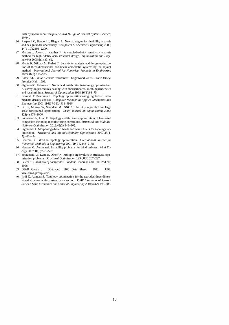
We consider the optimal design of a cantilever beam of con-stant cross section. The beam finite element model is composedof 16 three-node quadratic beam finite elements correspondingto 198 degrees of freedom. The coordinate system, finite ele-ment mesh and dimensions of the rectangular cross section ordesign domain are presented in Figure 2. The cross sectionis meshed using 2116 four-node isoparametric finite elementscorresponding to 6627 degrees of freedom. The beam is 2.4 mwide, 2 m in height, and 20 m long. Two different materialshave been considered – an orthotropic and an isotropic mate-rial – with the mechanical properties presented in Table 1. Themechanical properties of the orthotropic material are based onthat of an E-glass reinforced Epoxy laminate (cf. Peters [38]).The mechanical properties of the isotropic material correspondto that of DIAB H100 PVC Core (DIAB [39]).

Nine candidate materials have been considered for all numer-ical experiments. The candidate materials are generated basedon the material properties of the orthotropic layer and isotropiccore material in Table 1. One of the candidates is the isotropicmaterial itself. The remaining eight candidate materials aregenerated by rotation of the orthotropic layer. The orientationof the orthotropic layer in the cross section plane is specifiedbased on the orientationαp of the fiber plane and the orienta-tion α f of the fibers in the plane, cf. Figure 3. The eight can-didate materials considered correspond to four different layeror fiber orientations – 0◦, 45◦, −45◦, and 90◦ – stacked in ei-ther an horizontal (0◦) or vertical (90◦) fiber plane . Henceforththe nomenclatureα f @αp will be used when referring to an or-thotropic candidate material. For example, a layer oriented at45◦ stacked on a vertical plane (90◦) is referred to as 45◦@90◦

(cf. Figure 4).

5.2. Optimization strategy

The first step in the optimization is to solve the unpenalizedproblem corresponding to the case wherep = 1 in (7). At eachof the subsequent steps, the penalty parameterp is increasedby ∆p until p = pmax. For all numerical experiments presentedhere it is assumed that∆p = 0.5 andpmax= 5. Furthermore, forall cases, at the starting point all materials have the same vol-ume fractions. The optimal design problems are solved usingthe sequential quadratic programming algorithmsnopt by Gillet al. [32]. Each problem is solved until the major optimalitytolerance is satisfied or the maximum number of major itera-tions is reached. The major optimality tolerance, like the majorfeasibility tolerance, is set to 1× 10−5 in snopt. The maximumnumber of major iterations is set to 500 in the first iterationandto 100 in the remaining. The remaining parameters are set to thedefault values. All numerical experiments are solved for 19044

6

design variables associated with the nine candidate materials ateach of the 2116 elements of the cross section. The filter radiusis set tofr = 0.15 for all numerical experiments. Furthermore,the value ofw indicates the fraction of the total weight whichis orthotropic material. An equality constraint is used fortheweight in order to avoid designs where only the isotropic ma-terial exists. Moreover, it is assumed that the eigenfrequencygroups used in conjunction with the KS function are subsets ofω determined in (4). The eigenfrequency groups are denotedωi, j =

{ωi , ..., ω j

}where the subscriptsi and j indicate the order

of the lowest and higher eigenfrequencies in the group, respec-tively. The order number refers to the order placement inω.Only groups of consecutive eigenfrequencies have been con-sidered such thatωi, j includes the eigenfrequenciesi, j, andall eigenfrequencies in between. The value of the parameterβs

introduced in the definition of the KS function in (9) is set tounity for all cases. This ensures maximum numerical stabil-ity although the lower and upper bound of the eigenfrequencygroups estimated by the KS function may be overly conserva-tive. The sensitivity analysis technique for multiple eigenfre-quencies presented in Section 4.4 is employed whenever therelative difference between two or more eigenfrequencies is be-low 1× 10−5.

5.3. Presentation of the results

All numerical examples considered concern the optimal de-sign of prismatic beams, i.e., beam with constant cross sectionalong its length. Hence for each case the figures with the resultspresent only the cross section as this is sufficient to character-ize the optimal structural topology and material distribution ofthe entire beam. Two figures of the optimized cross sectionare presented for each case indicating the fiber and fiber planeorientation, respectively. The topology of the cross section isvisible in both. The fiber and fiber plane orientations are rep-resented by lines at each element. The thickness and darknessof the line is weighted by the value of the filtered design vari-able. It is possible in this way to visualize the effect of the filter.Based on the orientation of the lines and resorting to Figure4,it is possible to visualize the three-dimensional orientation ofthe fibers. The element is white if the material is isotropic.Theplots refer to the unpenalized filtered design variables. Finally,the position of the cross section reference point, shear center,and mass center is indicated in these group of figures with asquare, diamond, and triangle marker, respectively (cf. Figure4).

5.4. Results

All numerical experiments considered in this paper are de-fined in Table 2. The corresponding objective function and con-straint values for each of the numerical experiments are definedin Table 3. The optimized cross section topologies and materialdistribution are presented in Figures 5 and 7. The beam eigen-modes for a few relevant cases are presented in Figure 6 and 8.The eigenfrequencies, eigenmodes, constraint values, andnum-ber of objective function evaluations for each optimized designare presented in Table 4. For all cases the weight constraintis

satisfied and the shear center position constraint is activeat theoptimal design point. Furthermore, all values presented refer tothe penalized case, i.e.,p = pmax. The eigenmodes are iden-tified based on its predominant motion. Bending eigenmodeswith predominant displacements in thex and y direction areidentified asux anduy, respectively. The torsional eigenmodeassociated with rotation of the cross section around thezaxis isidentified asθz. The tension eigenmode involving displacementof the cross sections along thez axis is identified asuz. Thenotationu+xy andu−xy is used for bending eigenmodes whosepredominant displacementsx andy are of similar magnitude.Eigenmodes indicated byu+xy andu−xy have a predominant dis-placement going through the first and third, and second andfourth quadrants of thexy plane, respectively (see Figure 8).

The optimized beam cross section designs obtained for themaximization of the minimum eigenfrequency and maximiza-tion of the gap between eigenfrequencies – cases S1 and S2,respectively – are discussed first. The same formulations ex-tended to include a constraint on the shear center position –cases S3 and S4 – are discussed next.

5.4.1. Results without constraint on the shear center positionThe S1 case dealing with the maximization of the lowest

eigenfrequency and the cases S2-1, S2-2 and S2-3 addressingthe maximization of the gap between different groups of eigen-frequencies (cf. Table 2 and 3) are discussed in this section.The resulting cross section topology and material distributionfor cases S1 and S2 are presented in Figures 5(a-h). The lowestsix eigenfrequencies and predominant displacement of the cor-responding eigenvectors for each of the optimized beams arepresented in Table 4.

For case S1, the results in Table 4 show that the magnitudeof the two lowest eigenfrequencies are relatively similar andare associated with bending eigenmodes with predominant dis-placements in thex and y directions. The resulting box-liketopology in Figures 5(a-b) maximizes the moment of inertia andtherefore the bending stiffness of the beam in each of these di-rections. The fibers are aligned mostly along the beam lengthat 0◦@0◦ and 0◦@90◦ to maximize the bending stiffness. Inthe vertical or side faces,±45◦@90◦ fibers are visible at theheight of the horizontal neutral axis. These fibers resist theshear stresses induced by the transverse forces and contributeto an increase in shear stiffness in they direction and conse-quently of the lowest eigenfrequencyω1. This topology andmaterial distribution is similar to that obtained by Blasquesand Stolpe [11] for the minimum compliance optimization ofa square beam subjected to a vertical transverse load.

For cases S2-1, S2-2 and S2-3 the eigenfrequencies andeigenmodes indicated in Table 4 show that all optimized de-signs maximize the gap between a bending and torsion eigen-frequency. The eigenmodes for the bending eigenfrequencyω4

and torsional eigenfrequencyω5 for case S2-3 are presentedin Figure 6. Moreover, the progressive decrease in the mag-nitude of the lowest eigenfrequencies associated with bend-ing eigenmodes suggests that the optimized beams are progres-sively more compliant in bending for case S2-1, S2-2 and S2-3,respectively. In fact, Figures 5(a - h) show the transition from

7

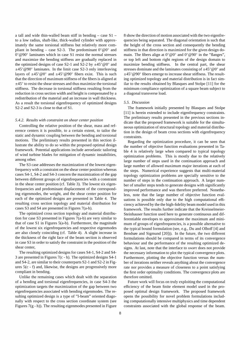
a tall and wide thin-walled beam stiff in bending – case S1 –to a low radius, shaft-like, thick-walled cylinder with approx-imately the same torsional stiffness but relatively more com-pliant in bending – case S2-3. The predominant 0◦@0◦ and0◦@90◦ laminates which in case S1 resist the normal stressesand maximize the bending stiffness are gradually replaced inthe optimized designs of case S2-1 and S2-2 by±45◦@0◦ and±45◦@90◦ laminates. In the limit case S2-3 only interleavinglayers of±45◦@0◦ and±45◦@90◦ fibers exist. This is suchthat the direction of maximum stiffness of the fibers is aligned at±45◦ to resist the shear stresses and thus maximize the torsionalstiffness. The decrease in torsional stiffness resulting from thereduction in cross section width and height is compensated by aredistribution of the material and an increase in wall thickness.As a result the torsional eigenfrequency of optimized designsS2-2 and S2-3 is close to that of S1.

5.4.2. Results with constraint on shear center position

Controlling the relative position of the shear, mass and ref-erence centers it is possible, to a certain extent, to tailorthestatic and dynamic coupling between the bending and torsionalmotions. The preliminary results presented in this sectionil-lustrate the ability to do so within the proposed optimal designframework. Potential applications include aeroelastic tailoringof wind turbine blades for mitigation of dynamic instabilities,among other.

The S3 case addresses the maximization of the lowest eigen-frequency with a constraint on the shear center position whereascases S4-1, S4-2 and S4-3 concern the maximization of the gapbetween different groups of eigenfrequencies with a constraintin the shear center position (cf. Table 3). The lowest six eigen-frequencies and predominant displacement of the correspond-ing eigenmodes, the weight, and the shear center position foreach of the optimized designs are presented in Table 4. Theresulting cross section topology and material distribution forcases S3 and S4 are presented in Figures 7(a-h).

The optimized cross section topology and material distribu-tion for case S3 presented in Figures 7(a-b) are very similartothat of case S1 in Figures 5(a-b). Furthermore, the magnitudeof the lowest six eigenfrequencies and respective eigenmodesare also closely coinciding (cf. Table 4). A slight increaseinthe thickness of the right face of the beam section is observedin case S3 in order to satisfy the constraint in the position of theshear center,

The resulting optimized designs for cases S4-1, S4-2 and S4-3 are presented in Figures 7(c - h). The optimized designs S4-1and S4-2, are similar to their counterparts S2-1 and S2-2 in Fig-ures 5(c - f) and, likewise, the designs are progressively morecompliant in bending.

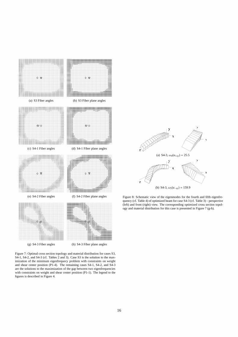
Unlike the remaining cases which dealt with the separationof a bending and torsional eigenfrequencies, in case S4-3 theoptimization targets the maximization of the gap between twoeigenfrequencies associated with bending eigenmodes. There-sulting optimized design is a type of ”I-beam” oriented diago-nally with respect to the cross section coordinate system (seeFigures 7(g - h)). The resulting eigenmodes presented in Figure

8 show the direction of motion associated with the two eigenfre-quencies being separated. The diagonal orientation is suchthatthe height of the cross section and consequently the bendingstiffness in that direction is maximized for the given design do-main. The fibers align at 0◦@0◦ and 0◦@90◦ in the ”flanges”,or top left and bottom right regions of the design domain tomaximize bending stiffness. In the central part, the shearstresses dominate and the laminates consisting of±45◦@0◦ and±45◦@90◦ fibers emerge to increase shear stiffness. The result-ing optimized topology and material distribution is in factsim-ilar to the results obtained by Blasques and Stolpe [11] for theminimum compliance optimization of a square beam subject toa diagonal transverse load.

5.5. DiscussionThe framework initially presented by Blasques and Stolpe

[11] is herein extended to include eigenfrequency constraints.The preliminary results presented in the previous sectionsin-dicate that the proposed framework is suitable for the simulta-neous optimization of structural topology and material distribu-tion in the design of beam cross sections with eigenfrequencyconstraints.

Regarding the optimization procedure, it can be seen thatthe number of objective function evaluations presented in Ta-ble 4 is relatively large when compared to typical topologyoptimization problems. This is mostly due to the relativelylarge number of steps used in the continuation approach andlarge number of allowed maximum major iterations at each ofthe steps. Numerical experience suggests that multi-materialtopology optimization problems are specially sensitive tothenumber of steps in the continuation approach. A larger num-ber of smaller steps tends to generate designs with significantlyimproved performance and was therefore preferred. Nonethe-less, note that the large number of objective function eval-uations is possible only due to the high computational effi-ciency achieved by the the high-fidelity beam model used in thisframework. The results further indicate that the Kreisselmeier-Steinhauser function used here to generate continuous and dif-ferentiable envelopes to approximate the maximum and mini-mum of groups of eigenfrequencies, is a possible alternative tothe typical bound formulation (see, e.g., Du and Olhoff [4] andBendsøe and Sigmund [20])). In the future, the two differentformulations should be compared in terms of its convergencebehaviour and the performance of the resulting optimized de-signs. At last, note that the interface tosnopt does not providethe necessary information to plot the typical convergence plots.Furthermore, plotting the objective function versus the num-ber of iterations neither reveals anything about the convergencerate nor provides a measure of closeness to a point satisfyingthe first order optimality conditions. The convergence plots aretherefore omitted.

Future work will focus on truly exploiting the computationalefficiency of the beam finite element model used in the pro-posed optimal design framework. The proposed frameworkopens the possibility for novel problem formulations includ-ing computationally intensive multiphysics and time dependentconstraints associated with the global response of the beam.

8

Moreover, a greater level of detail can be achieved by op-timizing a larger number of cross sections along the lengthof the beam to obtain a detailed three-dimensional design ofthe beam structure. Potential applications include the three-dimensional structural topology and material optimization ofwind turbine blades with aeroelastic stability and fatiguecon-straints. Nonetheless, despite the focus on the design of lam-inated composite beams, the framework is sufficiently generaland applicable to a broader class of problems dealing with thedistribution of multiple materials to optimize the performanceof beam-like structures. For example, the framework is wellsuited to topology optimization problems of beams with ex-trusion constraints. Typical approaches resort to computation-ally expensive three-dimensional solid finite element modelsand additional constraints on the design variables to ensure thatthe extrusion constraint is satisfied (see, e.g., Ishii and Aomura[40]). In this sense the approach proposed here has the poten-tial to allow for a significant improvement in terms of compu-tational efficiency.

6. Conclusions

A framework has been presented for the optimal design ofbeams with eigenfrequency constraints. The structural responseof the beam is analyzed using beam finite elements. The crosssection stiffness and mass properties are determined using a fi-nite element based cross section analysis tool. The resultingbeam model is able to account for effects stemming from ma-terial anisotropy and inhomogeneity in the analysis of beamswith arbitrary section geometry.

The optimal design problem is formulated in a multi-materialtopology optimization context. An alternative approach ispro-posed to handle the eigenfrequencies constraints based on theKreisselmeier-Steinhauser function.

Optimized cross section designs are presented for optimal de-sign problems dealing with the maximization of the minimumeigenfrequency and the maximization of the gap between con-secutive eigenfrequencies. Furthermore, results are alsopre-sented where the same problems are solved but the position ofthe shear center is constrained.

The numerical examples suggest that the devised optimal de-sign framework is suitable for the simultaneous optimizationof the cross section topology and material properties in thede-sign of laminated composite beams with stiffness and eigen-frequency constraints. The next step consists of applying thepresented methodology to the aeroelastic tailoring of laminatedcomposite wind turbine blades.

Acknowledgements

The author would like to thank Senior Scientist MathiasStolpe at Department of Wind Energy, Technical University ofDenmark, for all fruitful discussions and suggestions.

References

1. Diaz A, Kikuchi N. Solutions to shape and topology eigenvalue optimiza-tion problems using a homogenization method.International Journal forNumerical Methods in Engineering1992;35(7):1487–1502.

2. Ma Z, Kikuchi N, Hagiwara I. Structural topology and shapeoptimiza-tion for a frequency response problem.Computational mechanics1993;13:157–174.

3. Pedersen NL. Maximization of eigenvalues using topologyoptimization.Structural and multidisciplinary optimization2000;20(1):2–11.

4. Du J, Olhoff N. Topological design of freely vibrating continuum struc-tures for maximum values of simple and multiple eigenfrequencies andfrequency gaps. Structural and Multidisciplinary Optimization2007;34(2):91–110.

5. Luo J, Gea H. A systematic topology optimization approachfor opti-mal stiffener design.Structural and Multidisciplinary Optimization1998;16:280–288.

6. Gea H, Luo J. Automated Optimal Stiffener Pattern Design.Journal ofStructural Mechanics1999;27(3):275–292.

7. Stegmann J, Lund E. Discrete material optimization of general compositeshell structures.International Journal for Numerical Methods in Engi-neering2005;62(14):2009–2027.

8. Pedersen NL. On design of fiber-nets and orientation for eigenfrequencyoptimization of plates.Computational Mechanics2005;39(1):1–13.

9. Olhoff N. Optimization of vibrating beams with respect to higher ordernatural frequencies.Journal of Structural Mechanics1976;4:87–122.

10. Bendsøe MP, Olhoff N. A method of design against vibration resonanceof beams and shafts.Optimal Control Applications and Methods1985;6(3):191–200.

11. Blasques JP, Stolpe M. Multi-material topology optimization of lam-inated composite beam cross sections.Composite Structures2012;94(11):3278–3289.

12. Larsen T, Hansen A.How 2 HAWC2, the user’s manual. Denmark.Forskningscenter Risoe. Risoe-R. Risø National Laboratory; 2007. ISBN978-87-550-3583-6.

13. Blasques JP, Lazarov B.BECAS - A beam cross section analysis tool foranisotropic and inhomogeneous sections of arbitrary geometry. Risø-R1785 Technical Report; 2011.

14. Giavotto V, Borri M, Mantegazza P, Ghiringhelli G, Carmaschi V, Maf-fioli G, et al. Anisotropic beam theory and applications.Computers&Structures1983;16(1-4):403–413.

15. Jung S, Nagaraj V, Chopra I, Others . Assessment of composite rotorblade modeling techniques.Journal of the American Helicopter Society1999;44(3):188.

16. Volovoi V, Hodges D, Cesnik C, Popescu B. Assessment of beam mod-eling methods for rotor blade applications.Mathematical and ComputerModelling2001;33(10-11):1099–1112.

17. Hodges DH.Nonlinear composite beam theory; vol. 3. American Instituteof Aeronautics and Astronautics; 2006.

18. Hvejsel CF, Lund E. Material interpolation schemes for unified topologyand multi-material optimization.Structural and Multidisciplinary Opti-mization2011;43:811–825.

19. Hvejsel CF, Lund E, Stolpe M. Optimization strategies for discrete multi-material stiffness optimization. Structural and Multidisciplinary Opti-mization2011;44:149–163.

20. Bendsøe MP, Sigmund O.Topology optimization: theory, methods, andapplications. Springer Verlag; 2nd ed.; 2003. ISBN 3540429921.

21. Bendsøe MP, Kikuchi N. Generating optimal topologies instructural de-sign using a homogenization method.Computer Methods in Applied Me-chanics and Engineering1988;71:197–224.

22. Rozvany GI, Zhou M. The COC algorithm, Part I: Cross-section opti-mization or sizing.Computer Methods in Applied Mechanics and Engi-neering1991;89:281–308.

23. Bruns T, Tortorelli D. Topology optimization of non-linear elastic struc-tures and compliant mechanisms.Computer Methods in Applied Mechan-ics and Engineering2001;190(26-27):3443–3459.

24. Lund E, Stegmann J. On structural optimization of composite shell struc-tures using a discrete constitutive parametrization.Wind Energy2005;8(1):109–124.

25. Kreisselmeier G, Steinhauser R. Systematic control design by optimizinga vector performance index. In:International Federation of Active Con-

9

trols Symposium on Computer-Aided Design of Control Systems. Zurich;1979, .

26. Raspanti C, Bandoni J, Biegler L. New strategies for flexibility analysisand design under uncertainty.Computers& Chemical Engineering2000;24(9-10):2193–2209.

27. Martins J, Alonso J, Reuther J. A coupled-adjoint sensitivity analysismethod for high-fidelity aero-structural design.Optimization and Engi-neering2005;6(1):33–62.

28. Maute K, Nikbay M, Farhat C. Sensitivity analysis and design optimiza-tion of three-dimensional non-linear aeroelastic systemsby the adjointmethod. International Journal for Numerical Methods in Engineering2003;56(6):911–933.

29. Bathe KJ.Finite Element Procedures. Englewood Cliffs – New Jersey:Prentice Hall; 1996.

30. Sigmund O, Petersson J. Numerical instabilities in topology optimization:A survey on procedures dealing with checkerboards, mesh-dependenciesand local minima.Structural Optimization1998;16(1):68–75.

31. Borrvall T, Petersson J. Topology optimization using regularized inter-mediate density control.Computer Methods in Applied Mechanics andEngineering2001;190(37-38):4911–4928.

32. Gill P, Murray W, Saunders M. SNOPT: An SQP algorithm for largescale constrained optimization.SIAM Journal on Optimization2002;121(4):979–1006.

33. Sørensen SN, Lund E. Topology and thickness optimization of laminatedcomposites including manufacturing constraints.Structural and Multidis-ciplinary Optimization2013;48(2):249–265.

34. Sigmund O. Morphology-based black and white filters for topology op-timization. Structural and Multidisciplinary Optimization2007;33(4-5):401–424.

35. Bourdin B. Filters in topology optimization.International Journal forNumerical Methods in Engineering2001;50(9):2143–2158.

36. Hansen M. Aeroelastic instability problems for wind turbines.Wind En-ergy2007;10(6):551–577.

37. Seyranian AP, Lund E, Olhoff N. Multiple eigenvalues in structural opti-mization problems.Structural Optimization1994;8(4):207–227.

38. Peters S.Handbook of composites. London: Chapman and Hall; 2nd ed.;1998.

39. DIAB Group . Divinycell H100 Data Sheet. 2011. URLwww.diabgroup.com.

40. Ishii K, Aomura S. Topology optimization for the extruded three dimen-sional structure with constant cross section.JSME International JournalSeries A Solid Mechanics and Material Engineering2004;47(2):198–206.

10

7. Tables

11

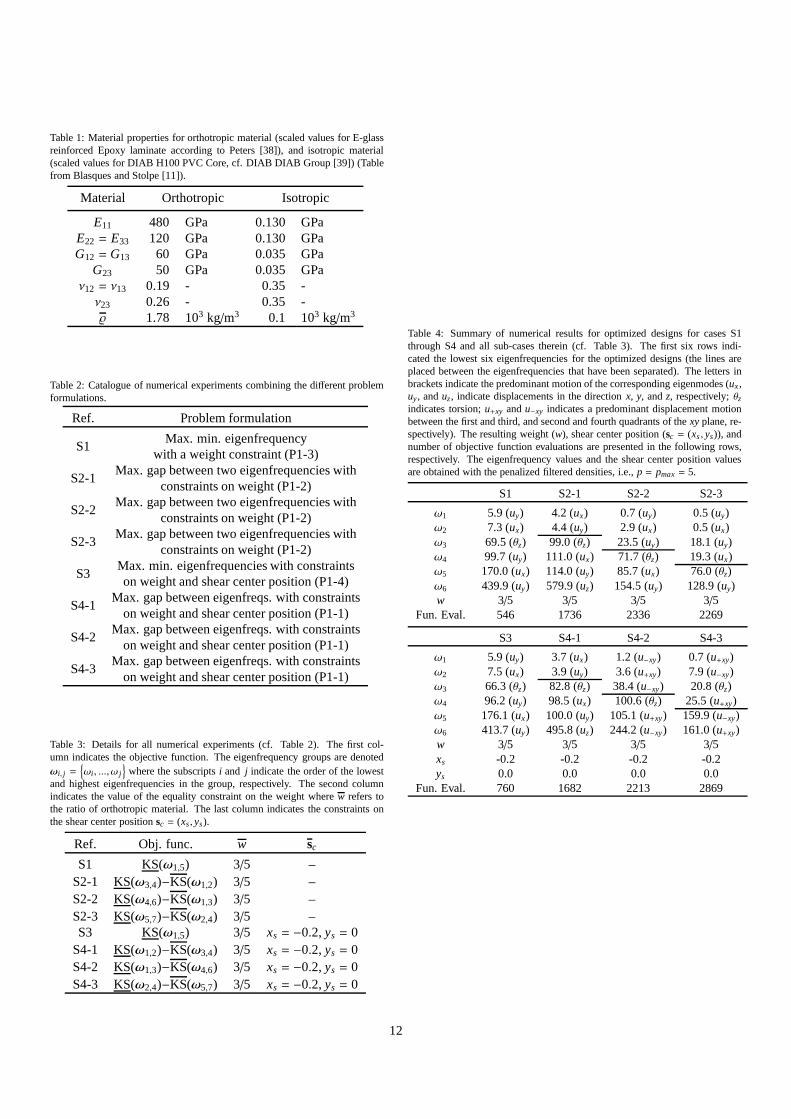
Table 1: Material properties for orthotropic material (scaled values for E-glassreinforced Epoxy laminate according to Peters [38]), and isotropic material(scaled values for DIAB H100 PVC Core, cf. DIAB DIAB Group [39]) (Tablefrom Blasques and Stolpe [11]).

Material Orthotropic Isotropic

E11 480 GPa 0.130 GPaE22 = E33 120 GPa 0.130 GPaG12 = G13 60 GPa 0.035 GPa

G23 50 GPa 0.035 GPaν12 = ν13 0.19 - 0.35 -ν23 0.26 - 0.35 - 1.78 103 kg/m3 0.1 103 kg/m3

Table 2: Catalogue of numerical experiments combining the different problemformulations.

Ref. Problem formulation

S1Max. min. eigenfrequency

with a weight constraint (P1-3)

S2-1Max. gap between two eigenfrequencies with

constraints on weight (P1-2)

S2-2Max. gap between two eigenfrequencies with

constraints on weight (P1-2)

S2-3Max. gap between two eigenfrequencies with

constraints on weight (P1-2)

S3Max. min. eigenfrequencies with constraintson weight and shear center position (P1-4)

S4-1Max. gap between eigenfreqs. with constraints

on weight and shear center position (P1-1)

S4-2Max. gap between eigenfreqs. with constraints

on weight and shear center position (P1-1)

S4-3Max. gap between eigenfreqs. with constraints

on weight and shear center position (P1-1)

Table 3: Details for all numerical experiments (cf. Table 2). The first col-umn indicates the objective function. The eigenfrequency groups are denotedωi, j =

{ωi , ..., ω j

}where the subscriptsi and j indicate the order of the lowest

and highest eigenfrequencies in the group, respectively. The second columnindicates the value of the equality constraint on the weightwherew refers tothe ratio of orthotropic material. The last column indicates the constraints onthe shear center positionsc = (xs, ys).

Ref. Obj. func. w sc

S1 KS(ω1,5) 3/5 –S2-1 KS(ω3,4)−KS(ω1,2) 3/5 –S2-2 KS(ω4,6)−KS(ω1,3) 3/5 –S2-3 KS(ω5,7)−KS(ω2,4) 3/5 –S3 KS(ω1,5) 3/5 xs = −0.2, ys = 0

S4-1 KS(ω1,2)−KS(ω3,4) 3/5 xs = −0.2, ys = 0S4-2 KS(ω1,3)−KS(ω4,6) 3/5 xs = −0.2, ys = 0S4-3 KS(ω2,4)−KS(ω5,7) 3/5 xs = −0.2, ys = 0

Table 4: Summary of numerical results for optimized designsfor cases S1through S4 and all sub-cases therein (cf. Table 3). The first six rows indi-cated the lowest six eigenfrequencies for the optimized designs (the lines areplaced between the eigenfrequencies that have been separated). The letters inbrackets indicate the predominant motion of the corresponding eigenmodes (ux,uy, anduz, indicate displacements in the directionx, y, andz, respectively;θzindicates torsion;u+xy andu−xy indicates a predominant displacement motionbetween the first and third, and second and fourth quadrants of the xyplane, re-spectively). The resulting weight (w), shear center position (sc = (xs, ys)), andnumber of objective function evaluations are presented in the following rows,respectively. The eigenfrequency values and the shear center position valuesare obtained with the penalized filtered densities, i.e.,p = pmax= 5.

S1 S2-1 S2-2 S2-3

ω1 5.9 (uy) 4.2 (ux) 0.7 (uy) 0.5 (uy)ω2 7.3 (ux) 4.4 (uy) 2.9 (ux) 0.5 (ux)ω3 69.5 (θz) 99.0 (θz) 23.5 (uy) 18.1 (uy)ω4 99.7 (uy) 111.0 (ux) 71.7 (θz) 19.3 (ux)ω5 170.0 (ux) 114.0 (uy) 85.7 (ux) 76.0 (θz)ω6 439.9 (uy) 579.9 (uz) 154.5 (uy) 128.9 (uy)w 3/5 3/5 3/5 3/5

Fun. Eval. 546 1736 2336 2269

S3 S4-1 S4-2 S4-3

ω1 5.9 (uy) 3.7 (ux) 1.2 (u−xy) 0.7 (u+xy)ω2 7.5 (ux) 3.9 (uy) 3.6 (u+xy) 7.9 (u−xy)ω3 66.3 (θz) 82.8 (θz) 38.4 (u−xy) 20.8 (θz)ω4 96.2 (uy) 98.5 (ux) 100.6 (θz) 25.5 (u+xy)ω5 176.1 (ux) 100.0 (uy) 105.1 (u+xy) 159.9 (u−xy)ω6 413.7 (uy) 495.8 (uz) 244.2 (u−xy) 161.0 (u+xy)w 3/5 3/5 3/5 3/5xs -0.2 -0.2 -0.2 -0.2ys 0.0 0.0 0.0 0.0

Fun. Eval. 760 1682 2213 2869

12

8. Figures

13

(a) Forces and moments(b) Strains and curva-tures

Figure 1: Cross section coordinate system, foces and moments (a), and corre-sponding strains and curvatures (b).

−1 −0.5 0 0.5 1−1

−0.5

0

0.5

1

x

y

Figure 2: Cross section coordinate system and finite elementmesh. The crosssection is meshed using 2116 four-node isoparametric finiteelements corre-sponding to 6627 degrees of freedom. The square marker indicates the positionof the cross section reference point or beam node.

Figure 3: Three-dimensional rotation of fiber plane and fiberorientation in thecross section mesh. The fiber plane orientation is defined by the angleαp whilethe orientation of the fibers in the fiber plane are defined by the angleα f . (Fig-ure from Blasques and Stolpe [11])

Fiber

orientation

Fiber plane

orientationSpatial

orientation

0o

0o

0o

0o

0o

90o

45o

-45o

90o

-45o

45o

90o

90o

90o

90o

0o

0o

90o

45o

-45o

0o

0o

0o

0o

@

@

@

@

+

+

+

+

=

=

=

=

90o

90o

90o

90o

0o

90o

45o

-45o

@

@

@

@

+

+

+

+

=

=

=

=

Orthotropic

Isotropic

CANDIDATE MATERIALS

CENTERS

Position of beam node Shear center Mass center

Figure 4: Legend for the figures depicting the solutions. Visualization of thespatial orientation of the fibers at each element based on theresulting fiberand fiber plane orientations, for each of the candidate orthotropic materials.Description of the markers used to define the cross section reference point orbeam node (square), shear center (diamond), and mass center(triangle). (Figurefrom Blasques and Stolpe [11])

14

(a) S1 Fiber angles (b) S1 Fiber plane angles

(c) S2-1 Fiber angles (d) S2-1 Fiber plane angles

(e) S2-2 Fiber angles (f) S2-2 Fiber plane angles

(g) S2-3 Fiber angles (h) S2-3 Fiber plane angles

Figure 5: Optimal cross section topology and material distribution for casesS1, S2-1, S2-2, and S2-3 (cf. Tables 2 and 3). Case S1 is the solution tothe maximization of the minimum eigenfrequecy problem witha weight con-straint (P1-3). The remaining cases S2-1, S2-2, and S2-3 arethe solutions to themaximization of the gap between two eigenfrequencies with weight constraints(P1-2). The legend to the figures is described in Figure 4.

(a) S2-3,ω4(ux) = 19.3 (b) S2-3,ω5(θz) = 76.0

Figure 6: Beam eigenmodes for the fourth and fifth eigenfrequency (cf. Table4) of optimized cantilever beam for case S2-3 (cf. Table 3). The correspond-ing optimized cross section topology and material distribution for this case ispresented in Figure 5 (g-h).

15

(a) S3 Fiber angles (b) S3 Fiber plane angles

(c) S4-1 Fiber angles (d) S4-1 Fiber plane angles

(e) S4-2 Fiber angles (f) S4-2 Fiber plane angles

(g) S4-3 Fiber angles (h) S4-3 Fiber plane angles

Figure 7: Optimal cross section topology and material distribution for cases S3,S4-1, S4-2, and S4-3 (cf. Tables 2 and 3). Case S3 is the solution to the max-imization of the minimum eigenfrequecy problem with constraints on weightand shear center position (P1-4). The remaining cases S4-1,S4-2, and S4-3are the solutions to the maximization of the gap between two eigenfrequencieswith constraints on weight and shear center position (P1-1). The legend to thefigures is described in Figure 4.

(a) S4-3,ω4(u+xy) = 25.5

(b) S4-3,ω5(u−xy) = 159.9

Figure 8: Schematic view of the eigenmodes for the fourth andfifth eigenfre-quency (cf. Table 4) of optimized beam for case S4-3 (cf. Table 3) – perspective(left) and front (right) view. The corresponding optimizedcross section topol-ogy and material distribution for this case is presented in Figure 7 (g-h).

16