Multi-Objective Optimisation Based on Relation Favour

Nicole Drechsler, Rolf Drechsler, Bernd Becker

Institute of Computer Science Albert-Ludwigs-University

79110 Freiburg im Breisgau, Germany email: ndrechsler,drechsler,becker@informatik.uni-freiburg.de

Abstract. Many optimisation problems in circuit design, in the following also refereed to as VLSI CAD, consist of mutually dependent sub-problems, where the resulting solutions must satisfy several requirements. Recently, a new model for Multi-Objective Optimisation (MOO) for applications in Evolutionary Algorithms (EAs) has been proposed. The search space is partitioned into so-called Satisfiability Classes (SCs), where each region represents the quality of the optimisation criteria. Applying the SCs to individuals in a population a fitness can be assigned during the EA run. The model also allows the handling of infeasible regions and restrictions in the search space. Additionally, different priorities for optimisation objectives can be modelled. In this paper, the model is studied in further detail. Various properties are shown and advantages and disadvantages are discussed. The relations to other techniques are presented and experimental results are given to demonstrate the efficiency of the model.

1 Introduction

Evolutionary Algorithms (EAs) become more and more important as a tool for search and optimisation. Especially for hard combinatorial problems they often have been applied successfully (see e.g. [Mic94,Dre98]). This type of problem is often encountered in Very Large Scale Integration CAD (VLSI CAD), since there often problem instances of several million components have to be considered. Multiple, competing criteria have to be optimised subject to a large number of non-trivial constraints. One strategy is to artificially divide a problem into a number of sub-problems, which are then solved in sequence. Obviously, this is not a promising strategy if the objectives are conflicting. EAs are well suited for solving this kind of problems, when mutually dependent sub-problems are considered in parallel. One problem that arises when using EAs is to evaluate the solutions of a population. Thus it is necessary to determine a ranking of the elements to see which solutions are better than others. Traditionally, the evaluation is done by an objective function which maps a solution of multiple objectives to a single value. A classical method is the linear combination by weighted sum, where the value of each objective is weighted by a constant coefficient. The values of the weights determine how strong the specific objective influences the value of a single fitness value. Disadvantages are that e.g. the weights have to be

known in advance to find good solutions or have to be determined by experiments. Obviously, this is time consuming and not desirable, since the parameters resulting from different runs may vary, ending in “in-stable” algorithms [Esb96].

1.1 Previous Work

Advanced methods for ranking solutions with multiple objectives have been developed over the years. If priorities exist between the objectives, a simple lexicographic order can be used. (Information on lexicographic sorting of vectors can be found in standard mathematical literature.) In [Gol89] a method is described where solutions with multiple objectives without preferences can be compared. This is realised by a relation, called dominate. A solution x dominates y, if x is equal or better for each objective than y, and x is for at least one component strongly better than y. Thus, the solutions in the search space can be ranked by the relation dominate. This approach of ranking solutions is the core of many EA-tools for Multi-Objective Optimisation (MOO) [SD95,FF95,ZT99]. In [EK96] another approach is proposed, where the search space is divided in a satisfiable, acceptable, and invalid range. This model has successfully been applied to one specific problem in the area of VLSI CAD, but it requires user interaction. The designer has to specify the limits between satisfiable, acceptable, and invalid solutions. The limits have to be adapted during the program run to obtain high quality results. Recently, in [DDB99] a new model for ranking solutions of MOO problems has been proposed. A relation favour is defined analogously to dominate in [Gol89]. The search space is divided into several Satisfiability Classes (SCs). Thus the approach can be seen as a generalisation of the approach in [EK96] using a finer granularity.

1.2 Results

In this paper the model from [DDB99] is studied in further detail. The relation favour in comparison to other models, like weighted sum and dominate [Gol89], is shown, e.g. favour is able to compare solutions which are not comparable using relation dominate. By this technique no user interaction is required any more. This is a very important aspect in VLSI CAD tools, since they are often so complex that it is very hard for a user to keep control. Furthermore, handling of priorities is also supported. Infeasible solutions are assigned to their own SCs depending on the objectives which are in an infeasible range. The SCs can be efficiently manipulated using operations on graphs. Finally, also experimental evaluations are given.

2 Multi-Objective Optimisation Problems

In general, many optimisation problems consist of several mutually dependent sub-problems. MOO problems can be defined as follows: Let ∏ be the feasible range of solutions in a given search space. The objective function fc : ∏ → Rn

+ assigns a cost to each objective of a solution s, where fc(s) = (fc1(s),fc2(s),…,fcn(s)), with s ∈ ∏, n ∈N and R+ the positive real valued numbers1. To compare several multi-objective solutions superior points in the search space can be determined. In the following we restrict to minimisation problems. The relation dominate is defined as proposed in [Gol89]. Let x, y ∈ Rn

+ be the costs of two different solutions. x dominates y (x <d y), if x ≠ y and y is as large as x in each component. More formally: Definition 2.1

x <d y : ⇔ ( ∃ i: fci(x) < fci(y)) ∧ (∀j ≠ i: fcj(x) ≤ fcj(y)) x ≤d y : ⇔ ( ∀ i: fci(x) ≤ fci(y))

A non-dominated solution is called a Pareto-optimal solution. ≤d defines the set of all Pareto-optimal solutions, called the Pareto-set, and additionally ≤d is a partial order. All elements x ∈ ∏ in the Pareto-set are equal or not comparable. Usually, all points in this set are of interest for the decision maker or designer.

3 The Model

We briefly review the model from [DDB99]. The main idea of the proposed model is to extend the approach from [EK96], such that the search space is divided into more than three categories, like e.g. superior, very good, good, satisfiable, and invalid. In the following the solutions are divided into so-called Satisfiability Classes (SCs) depending on their quality. The SCs are computed by a relation denoted favour, i.e. no limits have to be specified by user interaction. Solutions of “similar” quality belong to the same SC and thus each SC corresponds to a class of solutions of the same quality. After sorting the SCs with respect to their quality a ranking of the solutions is obtained. Let Π be a finite set of solutions and ∈n N. The objective function fc : Π → Rn

+ assigns a cost to each x ∈ Π as defined above. To classify solutions in SCs we define the relation favour (<f):

Definition 3.1

x <f y ⇔ |{i : fci(x) < fci(y), 1 ≤ i ≤ n}| > |{ j : fcj(x) < fcj(y), 1 ≤ j ≤ n }|

1 In general MOO problems the objective functions are not necessarily restricted to Rn

+, but it is convenient for our purposes.

4 Properties of Relation favour

We start with some general properties (that have partially already been observed in [DDB99]). Then we study the advantages and disadvantages in more detail and also focus on several properties of the model.

4.1 Basics

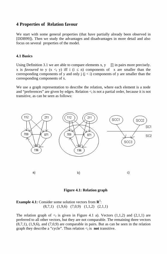
Using Definition 3.1 we are able to compare elements x, y ∈ ∏ in pairs more precisely. x is favoured to y (x <f y) iff i (i ≤ n) components of x are smaller than the corresponding components of y and only j (j < i) components of y are smaller than the corresponding components of x. We use a graph representation to describe the relation, where each element is a node and “preferences” are given by edges. Relation <f is not a partial order, because it is not transitive, as can be seen as follows:

Figure 4.1: Relation graph

Example 4.1: Consider some solution vectors from R3:

(8,7,1) (1,9,6) (7,0,9) (1,1,2) (2,1,1) The relation graph of <f is given in Figure 4.1 a). Vectors (1,1,2) and (2,1,1) are preferred to all other vectors, but they are not comparable. The remaining three vectors (8,7,1), (1,9,6), and (7,0,9) are comparable in pairs. But as can be seen in the relation graph they describe a ”cycle”. Thus relation <f is not transitive.

To get some more insight in the structure of the model we briefly focus on the meaning of the cycles in the relation graph: Elements are ranked equally when they are included in a cycle, because no element is superior to all the others. Elements that describe a cycle are denoted as not comparable. The determination of the Strongly Connected Components (SCC) of the relation-graph groups all elements which are not comparable in one SCC. The SCCs are computed by a DFS-based linear time graph algorithm [CLR90]. A directed graph GSC is constructed by replacing each SCC in G by one node representing this SCC. Thus, all cycles in G are eliminated. Let G = (V,E) be the graph that represents relation <f and a set of solutions and let Z be the set of SCCs in G, with Z=(Z1,…,Zr) and Zi = (Vi,Ei), 1 ≤ i ≤ r ≤ |V|. Let GZ = (VZ,EZ) be the graph where all SCCs Zi of G are replaced by a node vZi representing the SCC. An edge (vZi,vZj), 1 ≤ i,j ≤ r, i ≠ j, is set in GZ, if and only if there exists an edge (vk,vl) ∈ E, 1 ≤ k,l ≤ |V|, k ≠ l, with vk ∈ Zi and vl ∈ Zj, Zi ≠ Zj. It directly follows: Lemma 4.1: The directed graph GZ has no cycles. The relation that is described by the relation graph GZ is denoted by pf. Since GZ is acyclic, it is possible to determine a level sorting of the nodes. For each node in GZ we define a SC. Level sorting of the nodes in GZ determines the ranking of the SCs; each level contains at least one node of GZ. Then each level corresponds to exactly one SC. Using the level sorting it is possible to group nodes (set of solutions) that are not connected by an edge in the same SC. These solutions are not comparable with respect to relation pf and thus they should be ranked in the same level of quality. There are two possibilities to perform the level sorting:

1. starting with nodes v that have indegree(v) = 0 or 2. starting with nodes v that have outdegree(v) = 0. In the following the first strategy is used, since the best solutions that are not comparable should be placed in the same SC. Example 4.2: In Figure 4.1 b) SCC 1, SCC 2, and SCC 3 are illustrated. As can be seen the elements of SCC 1 and SCC 2 are superior to the elements of SCC 3. Figure 4.1 c) shows the relation graph GZ after level sorting. Level 1 corresponds to SC 1 and level 2 corresponds to SC 2. In the following some properties of relation favour are presented. For the case n = 2 it holds: Lemma 4.2: Let fc : Π → R2. Relations <d and pf are equal, i.e. for x, y ∈ Π it holds:

x <d y ⇔ x pf y Proof: Using Definition 3.1 with n = 2 it follows: Let i (j) ∈ N0 be the number of components of x (y) that are smaller than the corresponding components of y (x). Then

for x pf y and i and j it holds j < i ≤ 2 and i + j ≤ 2. Then for i and j it follows that i = 1 and j = 0 or i = 2 and j = 0. “⇒”: If x <d y, it follows i = 2 and j = 0 or i = 1 and j = 0 ⇒ x pf y “⇐”: Case 1: i = 1, j = 0 It follows: (x1 < y1) ∧ (x2 = y2) ⇒ x <d y Case 2: i = 2, j = 0 It follows: (x1 < y1) ∧ (x2 < y2) ⇒ x <d y �

Lemma 4.2 does not hold for n > 2 as can be stated by a counterexample: Example 4.3: Consider the vectors given in Example 4.1. Applying relation dominate vectors (1,1,2), (2,1,1) and (7,0,9) are not dominated by any other element; thus they are ranked as the best elements of the given vector set. In comparison to relation favour only the two vectors (1,1,2) and (2,1,1) are the best elements. For the computation of the execution time of the SCs an approximation can be given: Theorem 4.1: The computation time for the SC classification is O(|P|2⋅n).

Proof: Each element in a population P is compared to all other elements in P and in each comparison n components are tested. The number of nodes in the relation graph GZ is |P| and the operations on GZ have linear time complexity. Thus the computation time for the classification is O(|P|2⋅n). � First, we mention two points that should be considered when using the model. These points can be seen as disadvantages, if compared to other approaches. 1. Incomparable solutions may be placed in different SCs, even though there might be

cases where the user want them to be in the same class. 2. The different optimisation goals are considered in parallel and not relative to each

other (see also discussion below). But, the model has several advantages over other approaches: • No problem specific knowledge is needed for the choice of the weights of the fitness

function, like in the case of weighted sum. • Even if the components of a solution have different measures, a scaling of these

components is not needed, since there are no distances between the solutions computed (like e.g. using a weighted sum or information about distances between solutions).

• Dependent on the population the model dynamically adapts the relation graph that performs the comparison of the fitness function. In each generation the relation graph is re-computed and the ranking is updated. (This is done totally automatic and neither user interaction is required nor limits between the SCs have to be specified.) Thus, the granularity of the SCs is dynamically adapted to present conditions.

• Relation pf can also handle infeasible solutions. An infeasible component of the solution is considered as the worst possible value.

• If the structure of the search space changes during the EA run these changes are directly included in the relation that is updated online.

• Experiments have shown that the model results in a finer granularity than relation dominate.

• Due to the efficient representation based on graphs the run times are very low. • Handling of priorities of all (or some) objectives and of infeasible solutions is fully

supported. • No user interaction is required. This is very important in complex applications

where the user cannot keep control of all parameters by hand. In summary, there exist many advantages of the model compared to the “standard” techniques, which is demonstrated in the experiments. In the following some further scenarios are discussed that can occur in practice.

4.2 Sorting using Priorities

So far in the model it is not possible to handle priorities, e.g. to give a priority to the different optimisation criteria. This is not desired in most cases of complex applications, but we now outline how it can easily be added to the model as defined above. Let pr ∈ [0,1]m be the priority vector, where for each xi ∈ Π, pri denotes the priority of xi. The lower pri

is chosen, the higher is the priority of the corresponding component. If all values of pri’s are different, a lexicographic sorting can be used.

Components with same priority value are compared using relation pf . Only for these components a ranking is computed. Then based on this sorted set of elements a final ranking is determined by lexicographic sorting.

4.3 Invalid Solutions

The model is very well suited to handle invalid solutions. The classification, when an element is to be seen as “invalid” has to be defined by the user. The main idea is to modify the comparison operator. The invalid elements (for one or some specific components) always lose all comparisons carried out during the evaluation. I.e. if component xi, 1 ≤ i ≤ n, of vector x ∈ Rn

+ is invalid then it holds x > y for all valid y ∈ Π. This approach has been shown to work very well in practice.

4.4 Relation to Weighted Sum

Finally, we want to briefly comment on the relation of the model to the weighted sum approach, that is still used in many applications. The new model is not a cover of the weighted sum, i.e. the weighted sum cannot be embedded. The difference is that using

the presented model the solutions are ranked relatively to each other. Using the weighted sum the absolute values of each component are combined to determine a single fitness value. This is demonstrated by constructing an example: Example 4.4: Assume that the function f : R → R2 with f1(x) = x2 and f2(x) = (x-2)2 is given. If ω = (0.5,0.5) is the weight vector for the weighted sum, the minimal solution is x = 1 with f(x) = (1,1) and the corresponding weighted sum is 0.5⋅12+0.5⋅(1-2)2 = 1. It can be seen that for all other x values the sum is larger, e.g. the weighted sum of solutions x = 0 with f(x) = (0,4) and x = 2 with f(x) = (4,0) is 0.5⋅02+0.5⋅(0-2)2 = 2 and 0.5⋅22+0.5⋅(2-2)2 = 2 respectively. Using the above presented model it is not possible to perform a ranking such that (1,1) is better than solution (0,4) or (4,0). These three solutions are not comparable by relation favour.

5 Case Study: Heuristic Learning

Analogously to [DDB99] for carrying out experiments we choose the application “heuristic learning” of Binary Decision Diagram (BDD) [Bry86] variable orderings as proposed in [DB95,DGB96]. This application has been chosen due to several reasons:

• The problem has a high practical relevance and finds many applications in VLSI

CAD. • Due to the many studies already carried out, the problem is well understood. This

allows for clear interpretation of the results. • The problem is multi-objective in nature, i.e. quality (counted in number of nodes)

and run time has to be optimised.

To make the paper self-contained we review the main ideas from [DDB99].

5.1 The Learning Model

First, the basic learning model is briefly explained (for more details see [DB95,Dre00]). It is assumed that the problem to be solved has the following property: A non empty set of optimisation procedures can be applied to a given (non-optimal) solution in order to further improve its quality. These procedures are called Basic Optimisation Modules (BOMs). Each heuristic is a sequence of BOMs. The length of the sequence depends on the problem instances that are considered. The goal of the approach is to determine a good (or even optimal) sequence of BOMs such that the overall results obtained by the heuristic are improved. The set of BOMs defines the set H of all possible heuristics that are applicable to the problem to be solved in the given environment. H may include problem specific heuristics, local search operators but can also include some random operators. The individuals of our EA make use of multi-valued strings. The sequences of different length are modelled by a variable size representation of the individuals.

To each BOM h ∈ H we associate a cost function denoted by cost : H → R. cost estimates the resources that are needed for a heuristic, e.g. execution time of the heuristics. The quality fitness measures the quality of the heuristic that is applied to a given example.

Binary Decision Diagrams As well-known each Boolean function f : Bn → B can be represented by a Binary Decision Diagram (BDD), i.e. a directed acyclic graph where a Shannon decomposition is carried out in each node. We make use of reduced and ordered BDDs [Bry86]. We now consider the following problem that will be solved using EAs:

How can we develop a good heuristic to determine variable orderings for a BDD representing a given Boolean function f such that the number of nodes in the BDD is minimised?

Notice we do not optimise BDDs by EAs directly. Instead we optimise the heuristic that is applied to BDD minimisation.

Dynamic Variable Ordering The algorithms that are used as BOMs in the EA are based on dynamic variable ordering. Sifting (S) is a local search operation for variable ordering of BDDs which allows hill climbing. Sift light (L) is a restricted form of sifting, where hill climbing is not allowed. The third BOM is called inversion (I) which inverts the variable ordering of a BDD. For more details see [DGB96,Dre00].

5.2 Evolutionary Algorithm

The configuration of the EA is described in the following sections.

Representation In our application we use a multi-valued encoding, such that the problem can easily be formulated. Each position in a string represents an application of a BOM. Thus, a string represents a sequence of BOMs which corresponds to a heuristic. The size of the string has an upper limit of size lmax which is given by the designer and limits the maximum running time of the resulting heuristics. In the following we consider four-valued vectors: S (L, I) represents sifting (sift light, inversion) and value N denotes no operation. It is used to model the variable size of the heuristic.

Objective Function As an objective function that measures the fitness of each element we apply the heuristics to k benchmark functions in a training set T = {b1, … ,bk}. The quality of an individual is calculated by constructing the BDD and counting the number of nodes for each bi, 1 ≤ i ≤ k. Additionally, the execution time (measured in CPU seconds) that is

used for the application of the newly generated heuristic is minimised. Then, the objective function is a vector of length k+1 and is given by:

fc(T)=(#nodes(b1), … , #nodes(bk), time(T)),

where #nodes(bi), 1 ≤ i ≤ k, denotes the number of BDD nodes that are needed to represent function bi. The execution time that is needed to optimise all functions of the considered training set T is denoted by time. The choice of the fitness function largely influences the optimisation procedure. It is also possible to chose a fitness function as a vector of length 2!k by considering the execution time for each benchmark bi separately instead of using the sum. By our choice the EA focuses more on quality of the result than on the run time needed.

Algorithm 1. The initial population P is randomly generated. 2. Then P/2 elements are generated by the genetic operators reproduction and

crossover. The newly created elements are then mutated. 3. The offspring is evaluated. Then the new population is sorted using relation favour. 4. If no improvement is obtained for 50 generations the algorithm stops. For more details about the algorithm see [DGB96].

6 Experimental Results

All experiments in the following are carried out on a SUN Sparc 20 using the benchmark set from [Yan91].

First, the proposed model is compared to the weighted sum approach, because this is a “classical” method and used in many applications. Then a comparison to the “pure” Pareto-based approach from [Gol89] is performed. Notice, that comparisons to other approaches, as presented in [ZT99], are not given, because there the users’ interaction is required, e.g. if distances between solutions are computed.

6.1 Comparison to Weighted Sum

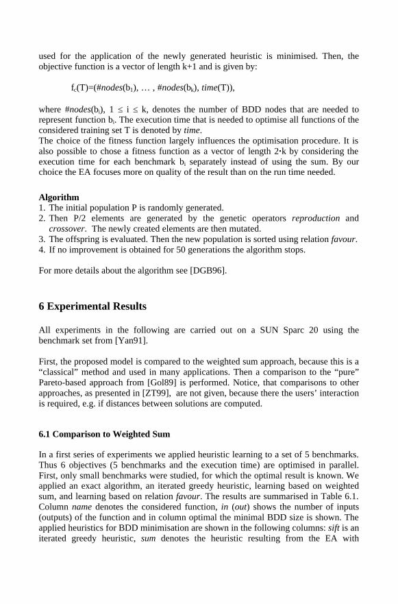
In a first series of experiments we applied heuristic learning to a set of 5 benchmarks. Thus 6 objectives (5 benchmarks and the execution time) are optimised in parallel. First, only small benchmarks were studied, for which the optimal result is known. We applied an exact algorithm, an iterated greedy heuristic, learning based on weighted sum, and learning based on relation favour. The results are summarised in Table 6.1. Column name denotes the considered function, in (out) shows the number of inputs (outputs) of the function and in column optimal the minimal BDD size is shown. The applied heuristics for BDD minimisation are shown in the following columns: sift is an iterated greedy heuristic, sum denotes the heuristic resulting from the EA with

weighted sum and f1 and f2 are the two alternative heuristics resulting from the EA using relation favour for ranking the individuals.

name in out optimal sift sum f1 f2add6 12 7 28 54 28 28 28

addm4 9 8 163 163 163 163 163 cm85a 11 3 27 35 27 27 30 m181 15 9 54 56 54 54 54 risc 8 31 65 65 65 65 65

average time > 100 0,4 1,6 0,9 0,4

Table 6.1

Regarding quality of course the exact algorithm determines the best results, but the run time is more then 100 CPU seconds. Iterated greedy is in some cases more than 30% worse than the exact result. Both learning approaches determine the same (optimal) quality, but the run time of the heuristic constructed by relation favour is nearly two times faster.

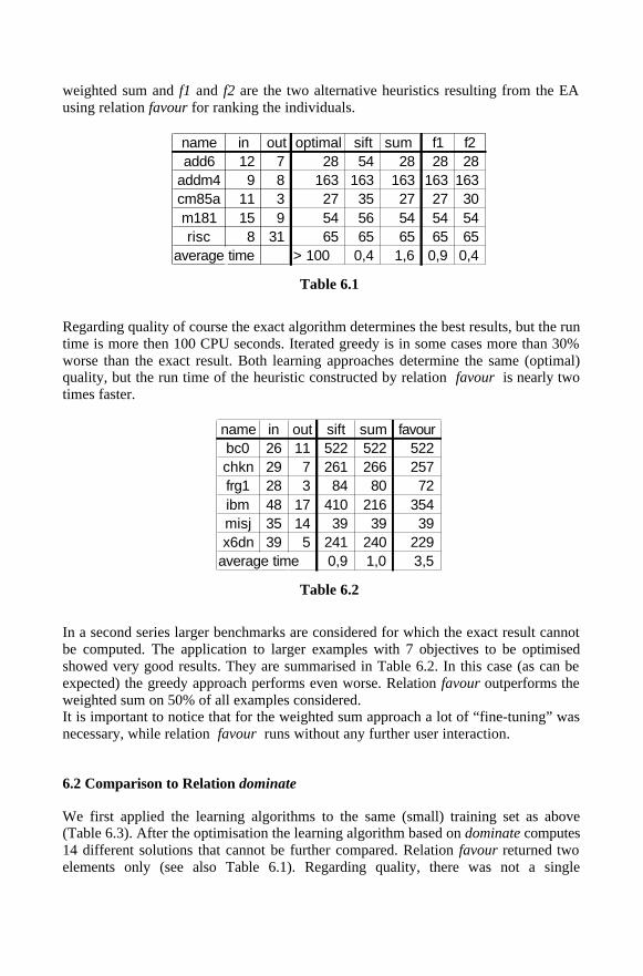
name in out sift sum favourbc0 26 11 522 522 522 chkn 29 7 261 266 257 frg1 28 3 84 80 72 ibm 48 17 410 216 354 misj 35 14 39 39 39 x6dn 39 5 241 240 229

average time 0,9 1,0 3,5

Table 6.2

In a second series larger benchmarks are considered for which the exact result cannot be computed. The application to larger examples with 7 objectives to be optimised showed very good results. They are summarised in Table 6.2. In this case (as can be expected) the greedy approach performs even worse. Relation favour outperforms the weighted sum on 50% of all examples considered. It is important to notice that for the weighted sum approach a lot of “fine-tuning” was necessary, while relation favour runs without any further user interaction.

6.2 Comparison to Relation dominate

We first applied the learning algorithms to the same (small) training set as above (Table 6.3). After the optimisation the learning algorithm based on dominate computes 14 different solutions that cannot be further compared. Relation favour returned two elements only (see also Table 6.1). Regarding quality, there was not a single

component where one of the 14 elements outperformed one of the two. Beside this the learning time for the algorithm based on favour was more than four times faster, i.e. 2.5 CPU hours instead of 14.

name in out d1 d2 d3 d4 d5 d6 d7 d8 d9 d10 d11 d12 d13 d14 f1 f2

add6 12 7 42 63 30 62 260 256 300 185 256 132 52 67 51 310 28 28

addm4 9 8 163 191 163 187 245 198 189 181 198 231 201 167 163 206 163 163

cm85a 11 3 33 39 35 30 37 37 43 39 46 49 30 35 33 37 27 30

m181 15 9 60 74 54 55 87 87 84 74 80 83 54 60 61 86 54 54

risc 8 31 70 71 65 66 94 79 84 95 97 94 65 65 65 90 65 65

average time 1,9 1,8 2,5 1,9 1,2 1,2 1,2 1,2 1,2 1,2 2,7 1,9 3,3 1,2 0,9 0,4

Table 6.3

When applying heuristic learning to construct heuristics in VLSI CAD it is very important that the number of final solutions is not too large, since finally the designer has to choose one. If the list becomes too long, it is not feasible to test them all, since the designs are too large. To further study the selection process, we finally applied our technique to a larger training set, where the algorithm based on relation dominate computed 16 solutions. To this result we applied the relation favour and this reduced the set to one element. More details are given in [Dre00].

6.3 Further Applications

In the meantime, the MOO model based on relation favour has been used in many projects and has been included in the software environment GAME (Genetic Algorithm Managing Environment) – a software tool developed for applications in VLSI CAD using evolutionary techniques. A method for test pattern generation for digital circuits and a tool for detailed routing of channels and switchboxes has been developed underlining the flexibility of the model (see [Dre98]).

7 Conclusion

Recently, in [DDB99] a new model for Multi-Objective Optimisation has been proposed that overcomes the limitations of classical EA approaches that often require several runs to determine good starting parameters. Furthermore, the model gives very robust results since the number of parameters is reduced without reducing the quality of the result. Only “non-promising'” candidates (for which can be guaranteed that they are not optimal and already better individuals exist) are not considered.

In this paper, we gave a detailed description of the model. Several properties have been discussed and advantages and disadvantages are described. We especially compared from a theoretical and practical point of view the relation of the new model to the weighted sum approach and to the relation dominate, respectively. As an advantage it turned out that components with different measures do not have to be scaled. This is done automatically comparing elements with relation favour. This may result in significant speed-ups in EAs and simplifies the handling of the algorithms.

References

[Bry86] R.E. Bryant. Graph-based algorithms for Boolean function manipulation. IEEE Trans. on Comp., 35(8):677-691, 1986.

[CLR90] T.H. Cormen, C.E. Leierson, and R.C. Rivest. Introduction to Algorithms. MIT Press,

McGraw-Hill Book Company, 1990. [Dre00] N. Drechsler. Über die Anwendung Evolutionärer Algorithmen in Schaltkreisentwurf,

PhD thesis, University of Freiburg, Germany, 2000. [Dre98] R. Drechsler. Evolutionary Algorithms for VLSI CAD. Kluwer Academic Publisher,

1998. [DB95] R. Drechsler and B. Becker. Learning heuristics by genetic algorithms. In ASP Design

Automation Conf., pages 349-352, 1995. [DDB99] N. Drechsler, R. Drechsler, and B. Becker. Multi-objective optimization in

evolutionary algorithms using satisfiability classes. In International Conference of Computational Intelligence, 6th Fuzzy Days, LNCS 1625, pages 108-117, 1999.

[DGB96] R. Drechsler, N. Göckel, and B. Becker. Learning heuristics for OBDD minimization

by evolutionary algorithms. In Parallel Problem Solving from Nature, LNCS 1141, pages 730-739, 1996.

[Esb96] H. Esbensen. Defining solution set quality. Technical report, UCB/ERL M96/1,

University of Berkeley, 1996. [EK96] H. Esbensen and E.S. Kuh. EXPLORER: an interactive floorplaner for design space

exploration. In European Design Automation Conf., pages 356-361, 1996. [FF95] C.M. Fonseca and P.J. Fleming. An overview of evolutionary algorithms in

multiobjective optimization. Evolutionary Computation, 3(1):1-16, 1995. [Gol89] D.E. Goldberg. Genetic Algorithms in Search, Optimization & Machine Learning.

Addision-Wesley Publisher Company, Inc., 1989. [HNG94] J. Horn, N. Nafpliotis, and D. Goldberg. A niched pareto genetic algorithm for

multiobjective optimization. In Int'l Conference on Evolutionary Computation, 1994.

[Mic94] Z. Michalewicz. Genetic Algorithms + Data Structures = Evolution Programs. Springer-Verlag, 1994.

[SD95] N. Srinivas and K. Deb. Multiobjective optimization using nondominated sorting in

genetic algorithms. Evolutionary Computation , 2(3):221-248, 1995. [Yan91] S. Yang. Logic synthesis and optimization benchmarks user guide. Technical Report

1/95, Microelectronic Center of North Carolina, Jan. 1991. [ZT99] E. Zitzler and L. Thiele. Multiobjective evolutionary algorithms: A comparative case

study and the strength pareto approach. IEEE Trans. on Evolutionary Computation, 3(4):257-271, 1999.