multi-objective supply chain network design under demand...
TRANSCRIPT

© IEOM Society
Multi-Objective Supply Chain Network Design Under Demand
Uncertainity Using Robust Goal Programming Approach
Raghda Taha, Khaled Abdallah Department of Supply Chain Management
College of International Transport and Logistics, Arab Academy for Science, Technology and
Maritime Transport, Egypt [email protected] , [email protected]
Yomna Sadek, Amin El-Kharbotly, Nahid Afia Department of Design and Production Engineering
Faculty of Engineering, Ain Shams University, Egypt [email protected] , [email protected] , [email protected]
Abstract
Supply Chain Network design involves strategic decisions on the location of production, distribution facilities,
capacities and transportation quantities. Supply chains are subjected to different types of Disruptions. In this paper,
the disruptions in the demand side are considered. A robust optimization approach is developed for the supply chain
network design under demand uncertainty. The supply chain problem considered is a multi-product multi-period
multi-echelon. The problem is formulated as a multi-objective model and solved using Goal programming. The
objectives are to maximize contribution, minimize the investment and disruptions costs. Installment of production
modules incrementally based on the demand at each planning period has significant effect on reducing the total
investment of the supply chain and the savings depends on the value of applied interest rate. The results showed that
the design vary significantly with demand range of variability. The profit, contribution and total cost are highly
sensitive to the ratio between disruption losses and selling price.
Keywords Supply Chain, Disruption Management, Multi-objective, Demand uncertainty
1. Introduction Supply chain disruptions are unplanned and unanticipated events that disrupt the normal flow of goods and materials
within a supply chain and, as a consequence, expose firms within the supply chain to operational and financial risks
(Craighead et al. 2007). The disruptions can be classified into supply side disruptions, process disruptions, and
demand side disruptions. Demand uncertainty is considered a source of disruption and can be used as measure for
disruption quantification. Different techniques are used to model demand uncertainty. Among of these techniques is
the Stochastic Programming and fuzzy approaches. In stochastic approach, uncertain parameters are assumed to
follow a particular probability distribution. However, in many cases, full distributional information is unknown or
very hard to determine. (see El-Sayed et al. 2010). Robust Optimization modeling considers uncertainty in
parameters as deterministic uncertainty sets in which all possible values of these parameters reside. “Robust
optimization attempts to compute feasible solutions for a whole range of scenarios of the uncertain parameters,
while optimizing an objective function in a controlled and balanced way with respect to the uncertainty in the
parameters” (Akbari and Karimi 2015).
Different types of uncertainty may be due to uncertainty in demand, cost parameters, capacity requirements etc.
Akbari and Karimi (2015) addressed process uncertainty by proposing a robust optimization approach for the design
and planning of a multi-echelon, multi-product, multi-period supply chain network. The objective was to minimize
the sum of location, allocation, transportation, and inventory carrying costs. It was formulated as a mixed integer
linear programming problem. Two uncertainty sets were assumed for production capacity requirement of each
product. A simulation-based procedure was developed to determine appropriate uncertainty budgets which lead to
the robust solution of acceptable feasibility and good performance.
Jin et al. (2014) considered supply chain network design, under uncertain market demand and cost. They proposed
robust optimization which was divided into two parts. The first part was facility location decision using a tabu
Proceedings of the 2015 International Conference on Operations Excellence and Service Engineering
Orlando, Florida, USA, September 10-11, 2015
827
© IEOM Society
search algorithm. The second part was flow decision which was addressed using the all-or-nothing method to design
the capacity of the plant. The robust optimization model was not only capable of reducing the risk of market, but it
also was able to avoid the error from the shortage cost. Zokaee et al. (2014) addressed uncertainty in demand, supply
capacity and cost parameters (transportation and shortage cost). A base model that aimed to determine the strategic
location and tactical allocation decisions for a deterministic four-echelon supply chain was proposed. The model
was then extended to incorporate uncertainty in key input parameters using a robust optimization approach that
could overcome the limitations of scenario-based solution methods in a tractable way. The application of the
approach was investigated in an actual case study where real data was utilized to design a bread supply chain
network. Tian and Yue (2014) considered uncertain demand and cost scenarios in the p-robust supply chain network
design and suggested a framework to obtain the relative regret limit.
Hosseini et al. (2014) addressed uncertain customer demands and transportation costs for the design of a distribution
network problem in a three-echelon supply chain. A mixed integer linear programming model was extended in a
robust optimization framework and three heuristic approaches based on genetic and memetic algorithms and a
mathematical programming approach were developed to solve this problem. Bai and Liu (2014) considered
uncertain demands and transportation costs. The modeling approach selected was a fuzzy value-at-risk (VaR)
optimization model, in which the uncertain demands and transportation costs were characterized by variable
possibility distributions. The experimental results showed that the proposed parametric optimization method could
provide an effective and flexible way for decision makers to design a supply chain network. Rezapour et al. (2013)
proposed a method that included stochastic and robust models for designing the network structure of a three echelon
supply chain under random demands of markets and by considering disruption probabilities in the procurement
facilities and connecting links of the chain.
Ashayeri et al. (2014) formulated a mixed integer programming (MIP) model with specific downsizing features. It
maximized the utilization of investment resources through a combined operation of demand selection and
production assets reallocation. The corresponding robust counterparts of the MIP model were further developed
based on robust optimization techniques for dealing with uncertainties of demands and exchange rates.
Moreover, Pishvaee et al. (2011) tackled uncertainty of input data in a closed-loop supply chain network design
problem. First, a deterministic mixed-integer linear programming model was developed for designing a closed-loop
supply chain network. Then, the robust counterpart of the proposed mixed-integer linear programming model was
presented by using the recent extensions in robust optimization theory. The uncertain data were the quantity of
returned products from the first market customers, the demands of second market customers and the transportation
costs between facilities and they were assumed to be varied in an uncertain closed box set. The robustness of the
solutions obtained by the robust optimization model was compared to that generated by the deterministic mixed-
integer linear programming model in a number of realizations under different test problems. Computational results
showed the superiority of the proposed robust model in both handling the uncertain data and the robustness of
respective solutions against to the solutions obtained by the deterministic model. Hasani et al. (2012) considered
strategic closed-loop supply chain network design for perishable goods. The supply chain was multi-period, multi-
product, and multi-echelon. The uncertainty was considered in the demand and purchasing cost. The proposed
model was handled via an interval robust optimization technique. The computational results of solving the proposed
model via LINGO 8 had demonstrated efficiency of the proposed model in dealing with uncertainty in an agile
manufacturing context.
Hatefi and Jolai (2014) considered uncertain parameters and facility disruptions . A robust model for an integrated
forward-reverse logistics network design was proposed. The model was formulated based on a robust optimization
approach to protect the network against uncertainty. Furthermore, a mixed integer linear programming model with
augmented p-robust constraints was proposed to control the reliability of the network among disruption scenarios.
The objective function of the proposed model was minimizing the nominal cost, while reducing disruption risk using
the p-robustness criterion. Baghalian et al. (2013) considered demand-side and supply-side uncertainties
simultaneously. A stochastic mathematical formulation was developed for designing a network of multi-product
supply chains comprising several capacitated production facilities, distribution centers and retailers in markets under
uncertainty. A transformation based on the piecewise linearization method was developed to solve the model. Taha
et al. (2014) studied the plant disruption and their effect on the network reliability considering regret cost and
recovery cost. Genetic algorithm was used to solve the problem and the results showed that, disruption cos affect the
supply chain design for optimizing the total cost including disruption cost.
828
© IEOM Society
Most of the reviewed literature did not consider the uncertainty or variation in demand as a source of disruption. The
objective of this work is to study the effect of uncertainty of demand on the design of the supply chain network. A
multi-objective multi-period multi-echelon model is proposed to design supply chain using robust optimization for
uncertain demand. The model allows for the assignment of modulated facilities of different capacities every period.
Hence, investment cost considers time value of money. The performance of the solution is measured in terms of
total disruption cost. The mathematical model is made to optimize separately the investment cost and contribution.
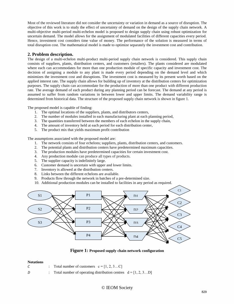
2. Problem description. The design of a multi-echelon multi-product multi-period supply chain network is considered. This supply chain
consists of suppliers, plants, distribution centers, and customers (retailers). The plants considered are modulated
where each can accommodates for more than one production module of specific capacity and investment cost. The
decision of assigning a module to any plant is made every period depending on the demand level and which
minimizes the investment cost and disruptions. The investment cost is measured by its present worth based on the
applied interest rate. The supply chain allows for building up of inventory at the distribution centers for optimization
purposes. The supply chain can accommodate for the production of more than one product with different production
rate. The average demand of each product during any planning period can be forecast. The demand at any period is
assumed to suffer from random variations in between lower and upper limits. The demand variability range is
determined from historical data. The structure of the proposed supply chain network is shown in figure 1.
The proposed model is capable of finding:
1. The optimal locations of the suppliers, plants, and distributors centers,
2. The number of modules installed in each manufacturing plant at each planning period,
3. The quantities transferred between the members of each echelon in the supply chain,
4. The amount of inventory held at each period for each distribution center,
5. The product mix that yields maximum profit contribution
The assumptions associated with the proposed model are:
1. The network consists of four echelons; suppliers, plants, distribution centers, and customers.
2. The potential plants and distribution centers have predetermined maximum capacities.
3. The production modules have predetermined capacities for certain investment cost.
4. Any production module can produce all types of products.
5. The supplier capacity is indefinitely large.
6. Customer demand is uncertain with upper and lower limits.
7. Inventory is allowed at the distribution centers.
8. Links between the different echelons are available.
9. Products flow through the network in batches of a pre-determined size.
10. Additional production modules can be installed to facilities in any period as required.
Figure 1: Proposed supply chain network configuration
Notations
𝐶 : Total number of customers c = [1, 2, 3…C]
𝐷 : Total number of operating distribution centres d = [1, 2, 3…D]
P2 S2 D2
P1 S1 D1
P4 D4
P3 S3 D3
C1
C2
C3
C4
C5
829

© IEOM Society
𝑀 : Total number of production modules m = [1, 2, 3…M]
𝑃 : Total number of operating plants p = [1, 2, 3…P]
𝑄 : Total number of products q = [1, 2, 3…Q]
𝑆 : Total number of suppliers s = [1, 2, 3…S]
𝑇 : Total number of planning periods t = [1, 2, 3…T]
𝑈 : Under capacity cost per unit for un-used capacity in plants
ℎ : Holding cost per unit
𝑟 : Interest rate
𝑆𝐶 : Losses per unit for shortage in customers’ demand
𝑂𝐶 : Losses per unit for over production than the customers’ demand
𝛿 : The range of variability
𝐴𝑣𝑔𝐷𝑒𝑚𝑐𝑞𝑡 : Average quantities of demand at customer (c) for product (q) at period (t)
𝐷𝑐𝑎𝑝d : Maximum capacity of distribution centre (d)
𝐷𝑒𝑚𝑐𝑞𝑡 : Uncertain demand at customer (c) for product (q) at period (t)
𝐹𝐶𝑑𝑑 : Fixed cost of operating distribution centre (d) per period
𝐹𝐶𝑚𝑚 : Fixed cost of operating production modules (m) per period
𝐹𝐶𝑝𝑝 : Fixed cost of operating plant (p) per period
𝑀𝑐𝑎𝑝mq : Capacity of production modules (m) to produce product (q)
𝑃𝐶𝑞 : Production cost per unit of product (q)
𝑃𝑐𝑎𝑝p : Maximum capacity of plant (p)
𝑆𝑃𝑞 : Selling price per unit of product (q)
𝑇𝑑𝑐𝑑𝑐 : Transportation cost of the link between distribution centre (d) and customer (c) per unit product
𝑇𝑝𝑑𝑝𝑑 : Transportation cost of the link between plant (p) and distribution centre (d) per unit product
𝑇𝑠𝑝𝑠𝑝 : Transportation cost of the link between supplier (s) and plant (p) per unit product
Decision Variables
𝑄𝑠𝑝𝑡𝑞𝑠𝑝 : Quantities of raw material for product (q) transported from supplier (s) to plant (p) at time period (t)
𝑄𝑝𝑑𝑡𝑞𝑝𝑑 : Quantities of product (q) transported from plant (p) to distribution centre (d) at time period (t)
𝑄𝑑𝑐𝑡𝑞𝑑𝑐 : Quantities of product (q) transported from distribution centre (d) to customer (c) at time period (t)
𝑄𝑝𝑟𝑜𝑑𝑡𝑞𝑝 : Quantities of products (q) produced at plant (p) at time period (t)
𝑄𝑖𝑛𝑣𝑡𝑞𝑑 : Quantities of products (q) stored at distribution centre (d) at time period (t)
𝑋𝑝𝑝𝑡 : Binary variable for plant (p) at period (t) {
1 𝑜𝑝𝑒𝑛0 𝑐𝑙𝑜𝑠𝑒𝑑
𝑋𝑑𝑑𝑡 : Binary variable for distribution centre (d) at period (t) ) {
1 𝑜𝑝𝑒𝑛0 𝑐𝑙𝑜𝑠𝑒𝑑
𝑌𝑚𝑚𝑝𝑡 : Number of production modules of type (m) installed in plant (p) at period (t)
3. Model objectives and constraints The proposed model considers three objectives. (1) minimizing the investment cost, (2) maximizing the
contribution, and (3) minimizing the disruption cost.
The investment cost is the sum of fixed costs from opening the plants and its modules, and distribution centers.
Since it is allowed to increase the production modules of plants in the future, the investment cost accounts
considering time value of money and interest rate. The first objective given in equation (1) .
Investment cost = ∑ ∑FCpp ∙ Xppt
(1 + r)t
P
p=1
T
t=1
+ ∑ ∑FCdd ∙ Xddt
(1 + r)t
D
d=1
T
t=1
+ ∑ ∑ ∑FCmm ∙ Ymmpt
(1 + r)t
M
m=1
P
p=1
T
t=1
(1)
830
© IEOM Society
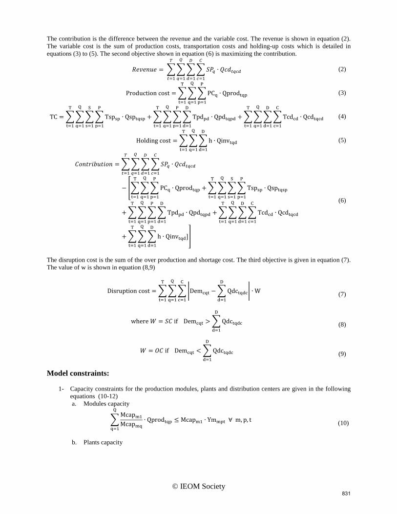
The contribution is the difference between the revenue and the variable cost. The revenue is shown in equation (2).
The variable cost is the sum of production costs, transportation costs and holding-up costs which is detailed in
equations (3) to (5). The second objective shown in equation (6) is maximizing the contribution.
𝑅𝑒𝑣𝑒𝑛𝑢𝑒 = ∑ ∑ ∑ ∑ 𝑆𝑃𝑞 ∙ 𝑄𝑐𝑑𝑡𝑞𝑐𝑑
𝐶
𝑐=1
𝐷
𝑑=1
𝑄
𝑞=1
𝑇
𝑡=1
(2)
Production cost = ∑ ∑ ∑ PCq ∙ Qprodtqp
P
p=1
Q
q=1
T
t=1
(3)
TC = ∑ ∑ ∑ ∑ Tspsp ∙ Qsptqsp
P
p=1
S
s=1
Q
q=1
T
t=1
+ ∑ ∑ ∑ ∑ Tpdpd ∙ Qpdtqpd
D
d=1
P
p=1
Q
q=1
T
t=1
+ ∑ ∑ ∑ ∑ Tcdcd ∙ Qcdtqcd
C
c=1
D
d=1
Q
q=1
T
t=1
(4)
Holding cost = ∑ ∑ ∑ h ∙ Qinvtqd
D
d=1
Q
q=1
T
t=1
(5)
𝐶𝑜𝑛𝑡𝑟𝑖𝑏𝑢𝑡𝑖𝑜𝑛 = ∑ ∑ ∑ ∑ 𝑆𝑃𝑞 ∙ 𝑄𝑐𝑑𝑡𝑞𝑐𝑑
𝐶
𝑐=1
𝐷
𝑑=1
𝑄
𝑞=1
𝑇
𝑡=1
− [∑ ∑ ∑ PCq ∙ Qprodtqp
P
p=1
Q
q=1
T
t=1
+ ∑ ∑ ∑ ∑ Tspsp ∙ Qsptqsp
P
p=1
S
s=1
Q
q=1
T
t=1
+ ∑ ∑ ∑ ∑ Tpdpd ∙ Qpdtqpd
D
d=1
P
p=1
Q
q=1
T
t=1
+ ∑ ∑ ∑ ∑ Tcdcd ∙ Qcdtqcd
C
c=1
D
d=1
Q
q=1
T
t=1
+ ∑ ∑ ∑ h ∙ Qinvtqd
D
d=1
Q
q=1
T
t=1
]]
(6)
The disruption cost is the sum of the over production and shortage cost. The third objective is given in equation (7).
The value of w is shown in equation (8,9)
Disruption cost = ∑ ∑ ∑ |Demcqt − ∑ Qdctqdc
D
d=1
|
C
c=1
Q
q=1
T
t=1
∙ W
(7)
where 𝑊 = 𝑆𝐶 if Demcqt > ∑ Qdctqdc
D
d=1
(8)
𝑊 = 𝑂𝐶 if Demcqt < ∑ Qdctqdc
D
d=1
(9)
Model constraints:
1- Capacity constraints for the production modules, plants and distribution centers are given in the following
equations (10-12)
a. Modules capacity
∑Mcapm1
Mcapmq
∙ Qprodtqp
Q
q=1
≤ Mcapm1 ∙ Ymmpt ∀ m, p, t
(10)
b. Plants capacity
831

© IEOM Society
∑ Mcapmq ∙ Ymmpt
M
m=1
≤ Pcapp ∙ 𝑋𝑝𝑝𝑡 ∀p, q, t (11)
c. Distribution centers capacity
∑ Qpdtqpd
P
p=1
+ Qinvtqd ≤ Dcapd ∙ 𝑋𝑑𝑑𝑡 ∀d, q, t
(12)
2- Balance constraints at the plants and the distribution centers are given in the following equations (13-14)
a. Balance at plants
Qprodtqp = ∑ Qpdtqpd
D
d=1
∀p, q, t
(13)
b. Balance at distribution centers
Qinv(t−1)qd + ∑ Qpdtqpd
P
p=1
= Qinvtqd + ∑ Qdctqdc
C
c=1
∀𝑝, 𝑞, 𝑡
(14)
3- Number of modules constraints ensures that the number of installed modules in next period (t+1) must be
greater than or equal to the number of modules in the current period (t)
Ymmpt ≤ Ymmpt+1 ∀t, p
(15)
4- Demand constraints; upper and lower demand limits under uncertainty
𝐷𝑒𝑚𝑐𝑞𝑡 < (1 + δ) ∙ 𝐴𝑣𝑔𝐷𝑒𝑚𝑐𝑞𝑡
(16)
𝐷𝑒𝑚𝑐𝑞𝑡 > (1 − δ) ∙ 𝐴𝑣𝑔𝐷𝑒𝑚𝑐𝑞𝑡 (17)
5- Non-negativity constraints
𝑄𝑠𝑝𝑡𝑞𝑠𝑝, 𝑄𝑝𝑑𝑡𝑞𝑝𝑑 , 𝑄𝑑𝑐𝑡𝑞𝑑𝑐 , 𝑄𝑝𝑟𝑜𝑑𝑡𝑞𝑝 , 𝑄𝑖𝑛𝑣𝑡𝑞𝑑 , 𝑌𝑚𝑚𝑝𝑡 , 𝑋𝑝𝑝𝑡 , 𝑋𝑑𝑑𝑡 ≥ 0 ∀f, d,c
(18)
6- Integer constraints are shown in equation (19)
7- Binary constraints for the plants and distribution centers locations
𝑋𝑝𝑝𝑡 , 𝑋𝑑𝑑𝑡 are binary ∀t, p, 𝑑
(20)
4. Computational results A set of experiments are designed and conducted to study the effectiveness of the proposed model. The assumed
supply chain design input data are given in Table 1. The proposed model is solved using FICO Xpress Optimization software. Robust optimization and goal programming modules are used to design the supply chain and analyze
experiments results at different conditions. All assumed goal programming objectives are given the same weight.
Disruption cost was the primary objective followed by the investment cost and the contribution.
Table 1 Data set for numerical example
Parameter Value
No. of potential suppliers (s) 3
𝑄𝑠𝑝𝑡𝑞𝑠𝑝
𝐵𝑎𝑡𝑐ℎ 𝑠𝑖𝑧𝑒,
𝑄𝑝𝑑𝑡𝑞𝑝𝑑
𝐵𝑎𝑡𝑐ℎ 𝑠𝑖𝑧𝑒,
𝑄𝑑𝑐𝑡𝑞𝑑𝑐
𝐵𝑎𝑡𝑐ℎ 𝑠𝑖𝑧𝑒,
, 𝑄𝑝𝑟𝑜𝑑𝑡𝑞𝑝
𝐵𝑎𝑡𝑐ℎ 𝑠𝑖𝑧𝑒, 𝑌𝑚𝑚𝑝𝑡 are integers ∀t, q, p, 𝑑, 𝑐 (19)
832
© IEOM Society
No. of potential plants (P) 4
No. of potential DCs (D) 4
No. of customers (C) 5
No. of Periods (T) 4
No. of products (Q) 2
Production Modules Module A and Module B
Module A capacity q1=100 , q2 =150
Module B capacity q1=200 , q2 =220
Investment cost per period for Module A 3000
Investment cost per period for Module B 4500
Cost of opening Plant (P) per Period 50 000
Cost of opening DC (d) per Period 20 000
𝑃𝑐𝑎𝑝p, 𝐷𝑐𝑎𝑝d 6000
Interest Rate 10%
Unit Price q1=150 , q2=160
Production cost q1=20 , q2=30
Transportation cost per unit per period 10
Holding Cost per unit per period 10
Over-capacity cost per unit per period 30
Penalty cost per unit per period 30
Customer mean demand during the first period 500 Unit
Increase in customer demand per period 100 unit
Variability range in demand ± 10%
5.1 The effects of the Demand Variability on the supply chain network design
The aim of this experiment is to study the effect of the demand disruptions on the supply chain network design. The
results shown in Table (2) indicate that the supply chain design changes every period with the increase in average
demand and demand range of variation.
Two cases are considered. The first case is the supply chain design with deterministic demand while the second case
is considering the variability in the demand as a disruption. For each period the design is given as the number of
plants and the number of modules installed in each plant. For example P1(17A, 14B) indicates that plant 1 is open
and 17 module of type A and 14 module of type B are installed. Also D1, D2 indicates that two distribution centers
are opened.
Table 2 Results of the generated test problems
Design at δ = 0 Design at δ = 0.1
Period 1:P1( 17A, 14B), D1, D2 Period 1:P1( 14A, 13B), D1, D2
Period 2:P1(18A, 15B), D1, D2 Period 2:P1(18A, 15B), D1, D2
Period 3:P1(18A, 15B), P2(0, 7B), D1, D2 Period 3:P1(18A, 15B), D1, D2
Period 4:P1(18A, 15B), P2(5A, 8B), D1, D2 Period 4:P1(18A, 15B), P2(9A, 3B), D1, D2
5.2 The effects of the Demand Variability
This experiment is to study the effect of the demand variability range on the different cost elements. The results
shown in Table 3 indicate that the cost elements vary considerably with demand variability ranges. For these test
problems all the parameters were kept fixed and δ is the only variable. It is evident that in general all financial
results slightly increase up to demand variation of 1% and then decrease except shortage and over production and
holding costs. It is worth mentioning that when optimizing the model by Integer Programming with no demand
variation (no disruption) same results given for δ =0 were obtained.
Table 3 Results of the generated test problems at different demand variability ranges at w/sp = 0.2
Parameter δ = 0 δ = 0.001 δ = 0.005 δ = 0.01 δ = 0.05 δ = 0.1
Revenue 4,030,000 4,036,200 4,051,700 4,055,650 3,899,000 3,691,500
Investment cost 703, 394 702,843 701,140 699,879 646,931 622717
833
© IEOM Society
Transportation cost 780,000 781,200 784,200 785,050 754,200 714000
Over-production cost 0 2,400 8,400 12,750 13,980 13560
Shortage cost 0 - 60 3,000 64,800 144000
Holding cost 2800 3,000 3,080 3,000 17,680 7160
Variable Cost 1,432,800 1,435,200 1,440,780 1,442,350 1,402,680 1,318,660
Contribution 2,597,200 2,601,000 2,610,920 2,613,300 2,496,320 2,372,840
Total cost 2,136,190 2,138,040 2,141,920 2,142,230 2,049,610 1,941,380
Profit 1,893,810 1,898,160 1,909,780 1,913,420 1,849,390 1,750,120
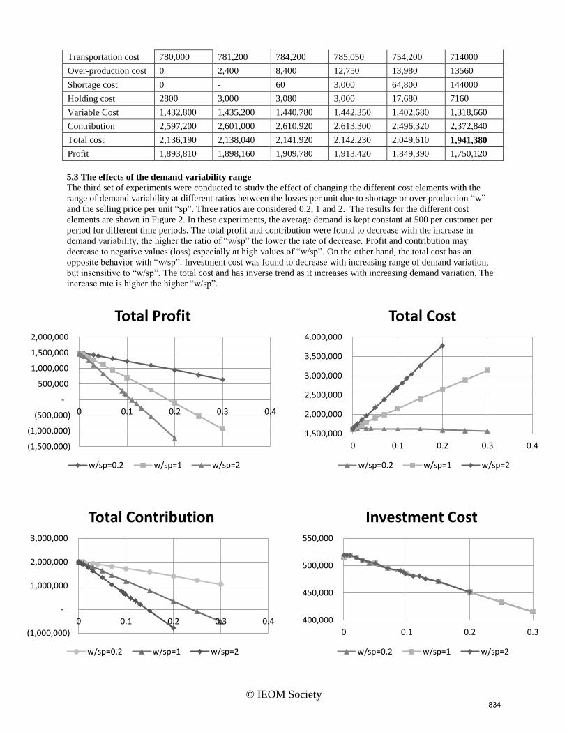
5.3 The effects of the demand variability range
The third set of experiments were conducted to study the effect of changing the different cost elements with the
range of demand variability at different ratios between the losses per unit due to shortage or over production “w”
and the selling price per unit “sp”. Three ratios are considered 0.2, 1 and 2. The results for the different cost
elements are shown in Figure 2. In these experiments, the average demand is kept constant at 500 per customer per
period for different time periods. The total profit and contribution were found to decrease with the increase in
demand variability, the higher the ratio of “w/sp” the lower the rate of decrease. Profit and contribution may
decrease to negative values (loss) especially at high values of “w/sp”. On the other hand, the total cost has an
opposite behavior with “w/sp”. Investment cost was found to decrease with increasing range of demand variation,
but insensitive to “w/sp”. The total cost and has inverse trend as it increases with increasing demand variation. The
increase rate is higher the higher “w/sp”.
(1,500,000)
(1,000,000)
(500,000)
-
500,000
1,000,000
1,500,000
2,000,000
0 0.1 0.2 0.3 0.4
Total Profit
w/sp=0.2 w/sp=1 w/sp=2
1,500,000
2,000,000
2,500,000
3,000,000
3,500,000
4,000,000
0 0.1 0.2 0.3 0.4
Total Cost
w/sp=0.2 w/sp=1 w/sp=2
(1,000,000)
-
1,000,000
2,000,000
3,000,000
0 0.1 0.2 0.3 0.4
Total Contribution
w/sp=0.2 w/sp=1 w/sp=2
400,000
450,000
500,000
550,000
0 0.1 0.2 0.3
Investment Cost
w/sp=0.2 w/sp=1 w/sp=2
834

© IEOM Society
Figure 2: effect of Variability range
5.4 The effect of interest rate
The fourth experiment is to study the effect of the interest rate. All the parameters are fixed and interest rate “ 𝑟"
changes from 0 to 25%. The results in Figure 4 show that the total cost and investment cost decrease with interest
rate while the profit increases. This is due to the fact that, at each period, the model opens plants or adds production
farcicalities to the existing plants as required satisfying the demand and its variation. The investment cost
represented by the present worth should decrease with the increase of interest rate.
Figure 3: effect of interest rate
5. Conclusion The proposed model is capable to consider continuous installment of production modules as the demand increases
with time and this has reduced considerably the investment cost represented by the present worth.
The results of robust optimization showed that as the demand variability increases the disruption cost increases and
by virtue the contribution decreases. However, the results obtained were conservative so as to lead to minimum
disruption cost compared with the no disruption case.
The ratio between the losses due to shortage/over-production and the selling price has a significant effect on the
contribution and the total cost. The higher the value of this ratio is the higher the cost and the lower the contribution.
However this ratio had no effect on the investment cost as the investment cost decrease with the increase in the
demand variability.
It was also proved that incase where the interest rate are high, the higher the saving in investment if the installments
are made on time of demand requirement.
REFERENCES A.A. Akbari and B. Karimi. 2015. A new robust optimization approach for integrated multi-echelon, multi-product,
multi-period supply chain network design under process uncertainty. International Journal of Advanced
Manufacturing Technology (2015).
J. Ashayeri, N. Ma, and R. Sotirov. 2014. Supply chain downsizing under bankruptcy: A robust optimization
approach. International Journal of Production Economics 154 (2014), 1–15.
A. Baghalian, S. Rezapour, and R.Z. Farahani. 2013. Robust supply chain network design with service level against
disruptions and demand uncertainties: A real-life case. European Journal of Operational Research 227, 1
(2013), 199–215.
X. Bai and Y. Liu. 2014. Robust optimization of supply chain network design in fuzzy decision system. Journal of
Intelligent Manufacturing (2014).
C.W.a Craighead, J.b Blackhurst, M.J.c Rungtusanatham, and R.B.d Handfield. 2007. The severity of supply chain
disruptions: Design characteristics and mitigation capabilities. Decision Sciences 38, 1 (2007).
M. El-Sayed, N. Afia, and A. El-Kharbotly. 2010. A stochastic model for forward-reverse logistics network design
under risk. Computers and Industrial Engineering 58, 3 (2010), 423–431.
A. Hasani, S.H. Zegordi, and E. Nikbakhsh. 2012. Robust closed-loop supply chain network design for perishable
goods in agile manufacturing under uncertainty. International Journal of Production Research 50, 16 (2012),
4649–4669.
-
500,000
1,000,000
1,500,000
2,000,000
2,500,000
0 0.05 0.1 0.15 0.2 0.25 0.3
Profit Total cost Investment cost
Investment cost
Total cost
Profit
835

© IEOM Society
S.M. Hatefi and F. Jolai. 2014. Robust and reliable forward-reverse logistics network design under demand
uncertainty and facility disruptions. Applied Mathematical Modelling 38, 9-10 (2014), 2630–2647.
S. Hosseini, R.Z. Farahani, W. Dullaert, B. Raa, M. Rajabi, and A. Bolhari. 2014. A robust optimization model for a
supply chain under uncertainty. IMA Journal of Management Mathematics 25, 4 (2014), 387–402.
M. Jin, R. Ma, L. Yao, and P. Ren. 2014. An effective heuristic algorithm for robust supply chain network design
under uncertainty. Applied Mathematics and Information Sciences 8, 2 (2014), 819–826.
M.S. Pishvaee, M. Rabbani, and S.A. Torabi. 2011. A robust optimization approach to closed-loop supply chain
network design under uncertainty. Applied Mathematical Modelling 35, 2 (2011), 637–649.
S. Rezapour, J.K. Allen, T.B. Trafalis, and F. Mistree. 2013. Robust supply chain network design by considering
demand-side uncertainty and supply-side disruption. Proceedings of the ASME Design Engineering Technical
Conference 3 A (2013).
R.B. Taha, K.S. Abdallah Y.M. Sadek, A.K. El-Kharbotly, N.H. Afia. 2014. Design of Supply Chain Networks with
Supply Disruptions using Genetic Algorithm. Proceedings of the POMS 25th Annual conference (2014).
J. Tian and J. Yue. 2014. Bounds of relative regret limit in p-robust supply chain network design. Production and
Operations Management 23, 10 (2014), 1811–1831.
S. Zokaee, A. Jabbarzadeh, B. Fahimnia, and S.J. Sadjadi. 2014. Robust supply chain network design: an
optimization model with real world application. Annals of Operations Research (2014). ACM Transactions on
Applied Perception, Vol. 2, No. 3, Article 1, Publication date: May 2010.
Biography Raghda B. Taha Assistant lecturer of Industrial Engineering at Arab Academy for science, Technology and
Maritime transport. She is a PhD student at faculty of engineering, ASU. She has a MSc in Industrial engineering.
Amin K. El-Kharbotly Prof. of industrial engineering, ASU. 45 years of teaching experience for graduate and post
graduate IE courses. Supervised a large number of M.Sc. & Ph.D. degrees. 4-years a visiting Prof. at the American
University in Cairo.
Yomna M. Sadek Assistant professor at the Design and Production Engineering Dept., Ain Shams University since
2010. She is interested in the field of industrial engineering since her graduation in 2000. Graduation project in the
field of production planning. M.Sc. in the field of robot scheduling. Ph.D. in the field of supply chain network
design.
Nahid H. Afia Professor of industrial engineering at Ain Shams University. Teaching courses: industrial
organization, engineering economy, project management, work study, consumer behaviour, and marketing.
Supervised many graduation projects in the field of IE. Supervisor of many M.Sc. and Ph.D. students.
Khaled S. Abdallah Assistant Professor in Industrial Engineering at college of international transport and logistics,
Arab Academy for science, Technology and Maritime transport . Head of the department of supply chain
management. Main researcher in projects funded by MiTAG and WLT in Milwaukee, WI, USA. Member in several
national projects funded by IMC in Cairo, Egypt.
836