multi-period, multi-product, aggregate production … review of business research vol. 6. no. 2....

World Review of Business Research

Vol. 6. No. 2. September 2016 Issue. Pp. 170 – 185

Multi-period, Multi-product, Aggregate Production Planning under demand uncertainty by considering Wastage Cost and

Incentives

Md. Mosharraf Hossain*, Khairun Nahar**, Salim Reza*** and Kazi Mohammad Shaifullah***

Aggregate production planning (APP) involves the simultaneous determination of company’s production, inventory and employment levels which fall between the broad decisions of long range planning and detailed short range planning. A mathematical model is formulated to investigate the optimal decision on each planning period. The goal is to minimize the total relevant costs considering time varying demand, unstable production capacity and work forces, inventory control, wastage reduction, and proper incentive for work force. Genetic Algorithm Optimization (GAO) approach and Big M method are used for solving a real time multi-product, multi-period aggregate production planning (APP) decision problem. The practicality of the proposed model is demonstrated through its application in solving an APP decision problem in an industrial case study. Required values of decision variables are obtained by both Big M method and genetic algorithm optimization model using TORA version 2.00, Feb. 2006 software and MATLAB R2011a software respectively. According to cost minimization objective of Aggregate production planning, genetic algorithm optimization results better than Big M method.

Field of Research: Management

1. Introduction Manufacturers use economic models and forecasting researches to organize a firm's life to respond to the inevitable changes of the broader economy. Production planning does this in response to changes in demand. Changing a company's production schedule on a moment’s notice can be expensive and lead to insecurity. Planning for changes in demand months in advance ensures that the change of production schedules can occur with little effort. Aggregate production planning is a general approach to altering a company's production schedule to respond to changes in demand. Aggregate production planning (APP) is a medium range capacity planning that typically encompasses a time horizon from 3 to18 months and is about determining the optimum production, work force and inventory levels for each period of planning horizon for a given set of production resources and constraints. Such planning usually involves one product or a family of similar products with small differences so that considering the problem from an aggregated viewpoint is justified. *Prof. Dr. Md. Mosharraf Hossain, Department of Industrial & Production Engineering, Rajshahi University of Engineering & Technology, Rajshahi-6204, Bangladesh. **Corresponding Author: Khairun Nahar, Assistant Professor, Department of Industrial & Production Engineering, Rajshahi University of Engineering & Technology, Rajshahi-6204, Bangladesh. Email: [email protected] ***Salim Reza and Kazi Mohammad Shaifullah, Department of Industrial & Production Engineering, Rajshahi University of Engineering & Technology, Rajshahi-6204, Bangladesh

mailto:[email protected]

Hossain, Nahar, Reza & Shaifullah

171

The goal of aggregate production planning (APP) is to set overall production levels for eachproduct category to meet the fluctuating or uncertain demands in near future while minimizing costs and to set policies and decisions about the issues of hiring, lay off, overtime, backorder, subcontracting and inventory for the efficient utilization of resources. APP is an important upper level planning activity in a production management system. Other forms of family disaggregation plans, such as master production schedule, capacity plan, and

material requirements plan all depend on APP in a hierarchical way. In previous work

typically the costs included in aggregate production planning are costs of production, inventory, sub-contracting, backlog, payroll, hiring, and regular-time and overtime. In some

research also consider the time value of money. In this study, an aggregate Production Planning model is formulated minimize the total production cost under demand uncertainty environment considering wastage cost and incentive for workforces which are not considered in production planning models in earlier research works. In this work, comparison in results is provided by using two different solution method named Genetic Algorithm and Big-M technique to understand whether meta-heuristic (i.e Genetic Algorithm) solution procedure provides best result or not. No such comparison is performed in earlier research works. This paper arranged as follows- Section 2 presents the literature review to identify the research scope on Aggregate Production Planning (APP). Section 3 explains the problem description and model formulation. In this section, the Mathematical Model for APP is explained in detail. Section 4 contains model implementation through data collection and explanation. Section 5 presents summarized results and Section 6 presents the conclusions of the study.

2. Literature Review Aggregate production planning is associated with the determination of inventory, production and work force levels to consider fluctuating demand needs over a planning horizon, which ranges from six months up to a year. Typically, the planning horizon includes the next seasonal peak in demand. The planning horizon can be divided into periods. For instance, a one-year planning horizon could consist of six one-month periods plus two three-month periods. We may consider a fixed value for the physical resources of the firm during the planning horizon of interest and the planning attempt is oriented towards the best utilization of those resources, given the external demand needs. Since it is usually impractical to consider every fine detail related to the production process while maintaining such a long planning horizon, it is obligatory to aggregate the information being processed. The aggregate production approach is forecasted on the existence of an aggregate unit of production, such as the “average" item, or in terms of weight, volume, production time, or dollar value. Plans are based on aggregate demand for one or more aggregate items. Once the aggregate production plan is created, constraints are applied on the detailed production scheduling process, which decides the specific quantities to be produced of each individual item. In this paper, Dotoli et al (2006) it is considered the optimization of integrated supply chain including raw materials supply, intermediate supply, manufacturing, distribution, retail and customers. Many companies have been trying to optimize their production and distribution systems separately, but using this approach limits any possible increase in profit it was stated by Park (2005). The goal of APP is normally to meet forecasted fluctuating demand requirements during a specific period in cost-effective manner. Typically costs include the costs of production, inventory, sub-contracting, backlog, payroll, hiring, and regular-time and overtime Silva e


172

(2006) and also in papers (Jung, 2005) propose a solution for integrated production and distribution planning in complicated environments where the objective is to maximize the total profit. APP has attracted considerable interest from both practitioners and academics. For solving APP problems, certain constraints are imposed which demand constraint optimization. Ioannis (2009) described a novel genetic algorithm for the problem of constrained optimization. His model was a modified version of the genetic operators namely crossover and mutation. These new version preserve the feasibility of the trial solutions of the constrained problem that are encoded in the chromosomes. Ramezanian et al. (2012) concentrated on multi-period, multi-product and multi-machine systems with setup decisions. In their study, they developed a mixed integer linear programming (MILP) model for general two-phase aggregate production planning systems. Due to NP-hard class of APP, they implemented a genetic algorithm and Tabu search for solving this problem. Meta-heuristic methods are used to solve NP-hard problems and due to NP-hard class of aggregate production planning, these approaches have been used for solving APP by Fahimniaet et al (2006) and Jiang et al (2008) and other method such as hybrid algorithm is used by Ganesh and Punniyamoorthy (2005); Kumar and Haq (2005), Baykasogluy (2006) and Pradenas and Pe-nailillo (2004) use Tabu search algorithm to solve APP models. Wang and Liang (2004) developed a fuzzy multi-objective linear programming (FMOLP) model for solving the multi-product APP decision problem in a fuzzy environment. The proposed model attempts to minimize total production costs, carrying and backordering costs and rates of changes in labor levels considering inventory level, labor levels, capacity, warehouse space and the time value of money. If decisions are made based on the deterministic model, there is a risk that demand might not be met with the right products. It is an unfortunate reality that some critical parameters such as customer demand, price and manufacturing capacity are not known with certainty. If the supply chain designed by the decision makers is not robust with respect to the uncertain environment, the impact of performance inefficiency (e.g. delay) could be devastating for all kinds of enterprises. Since they cannot usually protect themselves completely against the risk, they have to manage it. Risk management can be used as a tool for greater rewards, not just control against loss. There are lots of research work to deal with enterprise risk management by Wu and Olson (2008, 2009a, 2009b, 2010a, 2010b) and Wu et al (2010). Yeh and Chuang (2011) Four differences separate GAs from more traditional optimization techniques and those are, direct manipulation of a coding, searching from a population rather than a single point, following a blind searching technique and finally search using stochastic operators, not deterministic rules. It can be quite efficient to combine GA with other optimization methods. GA seems to be quite good for finding generally good global solutions, but quite inefficient at locating the last few mutations to determine the absolute optimum. Other techniques (such as simple hill climbing) are quite efficient at finding absolute optimum in a limited region. Alternating GA and hill climbing can improve the efficiency of GA while overcoming the lack of robustness of hill climbing. For solving Multiple Objective problems GA could generate the most optimum value. In Kazemi-Zanjani et al (2010) robust optimization approach was proposed as one of the potential methodologies to address MPMP production planning in a manufacturing environment with random yield. Ning et al (2006) considered multi product APP in fuzzy random environment. A fuzzy random APP model was established, in which the market demand, production cost, subcontracting cost, inventory carrying cost, backorder cost, product capacity, sales revenue, maximum labor level, maximum capital level, etc were all characterized as fuzzy random variables. Then a hybrid


173

optimization algorithm combining fuzzy random simulation, genetic algorithm (GA), neural network (NN) and simultaneous perturbation stochastic approximation (SPSA) algorithm was proposed to solve the model. Sharma and Jana (2009) Genetic Algorithm (GA) normally provides a series of alternative solutions for various GA parameter values. The decision-maker can find alternative optimal solutions from a series of alternative values. Bunnag and Sun (2005) presented a stochastic optimization method, referred to as a Genetic Algorithm (GA), for solving constrained optimization problems over a compact search domain. It was a real coded GA, which converges in probability to the optimal solution. The constraints were treated through a repair operator. A specific repair operator was included for linear inequality constraints. In contrast to aggregate-level plans, disaggregate-level plans conceptually provide each evacuee with unique staging and routing instructions, and thus these plans represent unstructured, split table, dynamic network flows through time. Disaggregate-level models are easier to formulate and solve than aggregate-level plans, for instance, many disaggregate-level models Chalmet (1982); Chiu (2007); Yao (2009); Bish (2011b) are formulated as linear programs (LPs) because of the continuous nature of their network flows. On the other hand, aggregate-level models are combinatorial in nature, and thus require binary decision variables and are formulated as more difficult-to-solve integer programs. Aggregate-level plans are, however, easier to implement in practice. When we solve APP problem, we have to face with uncertain market demands and capacities in production environment, imprecise process times, and other factors introducing inherent uncertainty to the solution. Ramazanian and Modares (2011) introduced a multi-objective goal programming model for a multi-product multi-step multi-period APP problem in the cement industry. The model was reformulated as a single objective nonlinear programming model. It was solved by using the expended objective function method and a propose PSO variant whose inertia weighted was set as a function. The simulation comparing with GA in the final showed that PSO gains satisfactory result then GA. Baltas et al (2013) introduced a PSO variant to a service design and diversification problem. They designed and implemented genetic algorithm and PSO to stated preference data derived from conjoint consumer preferences for service attributes in a retail setting. Their method has valuable implications for managers aiming to improve how they design their services. Liang (2007) introduced an interactive possibilistic linear programming (i-PLP) approach to solve multi-product and multi-time period APP problems with multiple imprecise objectives and cost coefficients by triangular possibility distributions in uncertain environments. The imprecise multi-objective APP model designed here seeks to minimize total production costs and changes in work-force level with reference to imprecise demand, cost coefficients, available resources and capacity. Additionally, the proposed i-PLP approach provides a systematic framework that helps the decision-making process to solve fuzzy multi-objective APP problems, enabling decision makers to interactively modify the imprecise data and parameters until a set of satisfactory solutions is derived. Paiva and Morabito (2009) proposed an optimization model to support decisions in the APP f sugar and ethanol milling companies. The model is a mixed integer programming formulation based on the industrial process selection and the production lot-sizing model. Also, in their APP real case study, the application of the model results in 12,306 variables, where 5796 are binary and 6902 constraints. Aliev et al (2007) developed a fuzzy integrated multi-period and multi-product aggregate production and distribution model in supply chain. The model was formulated in terms of fuzzy


174

programming and the solution was provided by genetic optimization (genetic algorithm). Ashayeri and Selen (2003) applied an APP model to make strategic planning decisions for the pharmaceutical industry in The Netherlands. Pega et al (2000) developed an integrated approach to address the aggregate planning problem and applied it to a firm, which yielded significant savings in the operational costs of the firm. In papers Disney et al (2004); Gaonkar and Viswanadham, (2005) the authors consider e-supply chain optimization between different stages of the chain, i.e. between suppliers and consumers, manufacturers and retailers. Feng and Rakesh (2010) considered an integrated optimization of logistics and production costs associated with the supply chain members based on the scenario approach to handle the uncertainty of demand. The formulation was a robust optimization model with expected total costs, cost variability due to demand uncertainty, and expected penalty. Andreas and Smith (2009) presented a model that considers aggregate-level routing where the evacuation routes for all sources combine to form a tree. Al-e-hashem et al (2013) consider transport mode decision variables (mode choice) to reduce GHGs and assume an interrelationship between lead time and transportation mode: the shorter the lead times, the more expensive transportation will be, while also increasing GHGs and waste management; obviously a supply chain is also characterized by the products it supplies. The point is that some products are friendlier to the environment than others. In other words, it is assumed that each unit of product is associated with a percentage of waste, and it limits the total amount of waste produced by each factory. Chakrabortty and Hasin (2013) presented an interactive MOGA approach to determine the optimum aggregate plan for meeting forecasted demand by adjusting regular and overtime production rates, inventory levels, labor levels, subcontracting and backordering rates, escalation factor in the each of the cost categories over a period of time and other controllable variables. Throughout the review, it is obvious that there have been a long phase for Aggregate production planning problem. All the previous works described in the above section gives descriptive knowledge on aggregate production planning study and all are relevant to real world problem. This study is oriented to a problem context, in which a manufacturer makes multiple products in various periods as the production capacities. In the previous works with GA for APP, there was only single application of escalating factors for certainty. The proposed approach attempts to evaluate the impact of escalating factor under uncertain demand but the paper Chakrabortty and Hasin (2013) evaluate impact of escalating factor under certain demand to minimize total costs. In general the factors considered for aggregate production planning are inventory levels, labor levels, overtime, subcontracting and backordering levels, labor level, machine, warehouse capacity. In paper Al-e-hashem et al (2013) wastage cost considered for transportation but in this study wastage cost include for total production cost which have an impact on total cost beside that incentive are also considered for the employees satisfaction. In this work a single objective approach is developed to minimize total costs in terms of inventory levels, labor levels, overtime, subcontracting and backordering levels, and labor, machine, warehouse capacity, incentive and wastage cost. In prior researches as mentioned above workforce incentive and production wastage cost with other previously mentioned costs in APP model is not included. In this work the aforementioned cost elements (that are the workforce incentive and production wastage cost) are consider to provide more sensible and relevant cost data. In this work, comparison in results is provided by using two different solution method named Genetic Algorithm and Big-M technique to test whether minimum total


175

cost is achieved by meta-heuristic algorithm named genetic algorithm or not, in compare with Big-M technique.

3. Problem Description & Model Formulation In the deterministic model, there is a risk that demand might not be met with the right products. It is an unfortunate reality that some critical parameters such as customer demand, price and manufacturing capacity are not known with certainty. If the production planning by the decision makers is not robust with respect to the uncertain environment, the impact of performance inefficiency (e.g. delay) could be devastating for all kinds of enterprises Wu and Olson (2008, 2009a, 2009b, 2010a, 2010b), Wu et. Al. (2010) This APP problem focuses on developing a single objective GA approach to determine the optimum aggregate plan for meeting uncertain demand by adjusting regular and overtime production rates, inventory levels, labor levels, subcontracting and backordering rates other controllable variables. In this model wastage cost and incentive are newly added. Wastage is costing real money and this is coming directly to increase total production cost, considering this issue waste cost is added in this problem. Due to inflation the time value of money decreases for this reason escalating factor is also considered. For the satisfaction of worker the incentive with regular & overtime production is also included in this APP problem. The multi-product, multi-period APP problem can be described as follows. Assume that a company manufactures N kinds of products to meet market demand over a planning horizon T. Assumptions- Based on the characteristics of the APP problem, the mathematical model will be constructed based on the following assumptions:

1. The values of all parameters are certain over the next T planning horizon except demand. 2. The escalating factors in each of the costs categories are certain over the next T planning horizon. 3. Actual labor levels, machine capacity and warehouse space in each period cannot exceed their respective maximum levels. 4. Uncertain demand is normally distributed with a mean & standard deviation. Notations-

The following notation is used after reviewing the literature and considering practical situations Chakrabortty, R. K. and Hasin, Md. A. A. (2013) & Al-e-hashem, S.M.J.M., Babolib, A., Sazvarb, Z. (2013)-

n=product type & t=period Dnt = Demand uncertain for nth product in period t (units) Rcnt = Regular time production cost per unit for nth product in period t (Tk. /unit) Rxnt= Regular time production of nth product in period t (units) ir = Escalating factor for regular time production cost (%) Ocnt = Overtime production cost per unit for nth product in period t (Tk. /unit) Oxnt= Overtime production of nth product in period t (units) io = Escalating factor for overtime production cost (%) Scnt = Subcontracting cost per unit of nth product in period t (Tk. /unit) Sxnt= Subcontracting volume of nth product in period t (units)


176

is = Escalating factor for subcontract cost (%) Icnt = Inventory carrying cost per unit of nth product in period t (Tk. /unit) Ixnt= Inventory level of nth product (units) in period tii = Escalating factor for inventory carrying cost (%) Bcnt = Backorder cost per unit of nth product in period t (Tk. /unit) Bxnt= Backorder level of nth product in period t (unit) ib = Escalating factor for backorder cost (%) Wcnt = Wastage cost per unit of nth product in period t (Tk. /unit) Wxnt= Wastage level of nth product in period t (unit) Wpnt= Percentage of wastage of nth product in period t (unit) Awnt= Allowable wastage produce in factory Tpnt= Targeted production for incentive of t period Tcnt=Cost of incentive of per unit product Tint = Amount of incentive level of nth product in period t (unit) Hct = Cost to hire one worker in period t (Tk. /man-hour) Ht = Worker hired in period t (man-hour) Fct = Cost to layoff one worker in period t (Tk. /man-hour) Ft = Workers laid off in period t (man-hour) if = Escalating factor for hire and layoff cost (%) Lnt = Hours of labor usage per unit of nth product in period t (machine-hour/unit) Mnt = Hours of machine usage per unit of nth product in period t (machine-hour/unit) Wnt = Warehouse spaces per unit of nth product in period t (ft2/unit) Ltmax = Maximum labor level available in period t (man-hour) Mtmax = Maximum machine capacity available in period t (machine-hour) Wtmax = Maximum warehouse space available in period t (ft2) Decision Variable-

Rxnt= Regular time production of nth product in period t (units) Oxnt= Overtime production of nth product in period t (units) Sxnt= Subcontracting volume of nth product in period t (units) Ixnt= Inventory level of nth product (units) in period t Bxnt= Backorder level of nth product in period t (unit) Wxnt= Waste level of nth product in period t (unit) Tint = Amount of incentive level of nth product in period t (unit) Ht = Worker hired in period t (man-hour) Ft = Workers laid off in period t (man-hour) Objective Function- Most practical decisions made to solve APP problems usually consider total costs. The proposed GA targeted the single objective function aims to minimize total cost of Aggregate Production Planning including production cost (regular time production cost, overtime production cost, subcontracting), labor cost (hiring cost, firing cost), inventory cost, shortage cost, wastage cost over the planning horizon T. Accordingly, the objective function of the proposed model is as follows:

Min, Z = ∑ (Ht. Hcttt=1 + Ft. Fct)(1 + if)

t + ∑ .tt=1 ∑ [IxntIcnt

nn=1 (1 + ii)

t + BxntBcnt(1 +ib)t+SxntScnt(1 + is)t + (WxntWcnt + TcntTint) +RxntRcnt(1 + ir)t + OxntOcnt(1 + io)t]; t= 1,2,3,…. T and n= 1,2,3,…N;


177

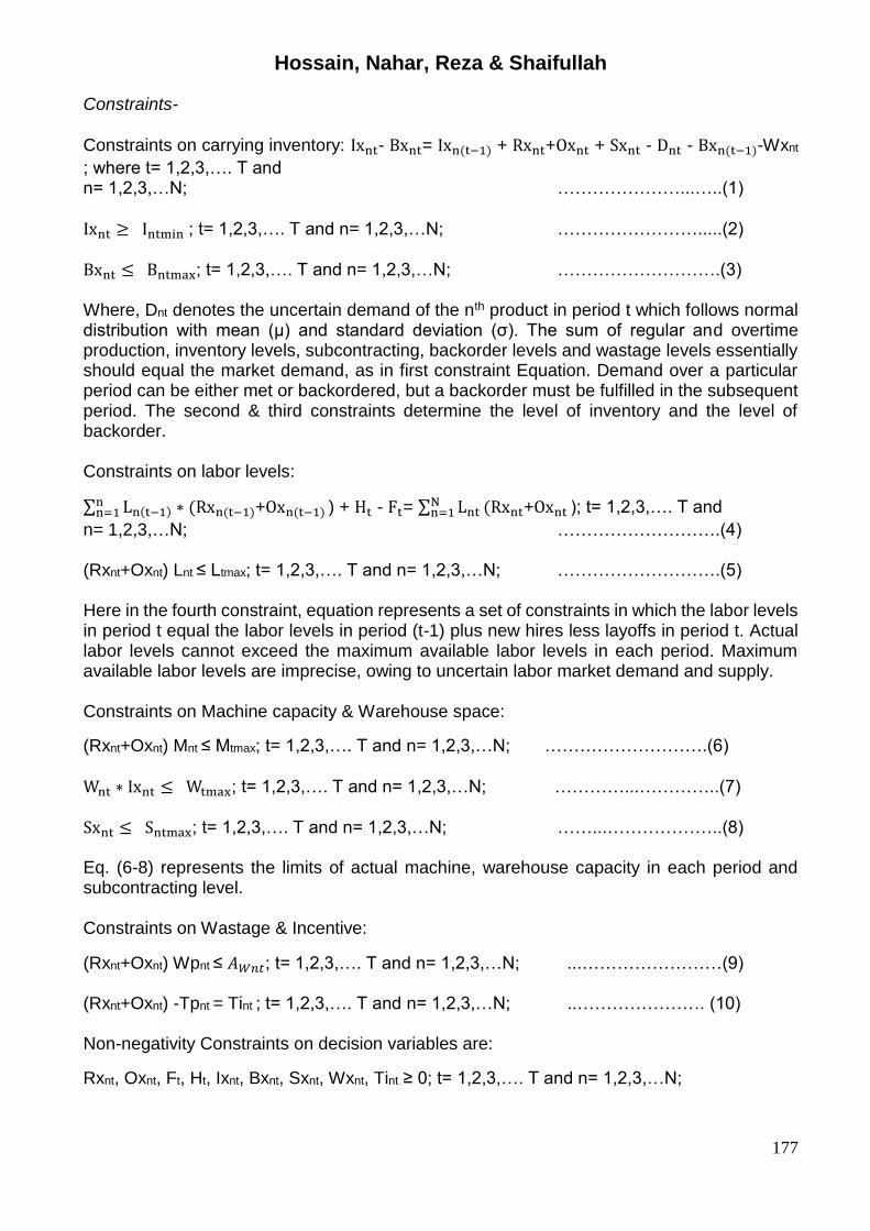
Constraints- Constraints on carrying inventory: Ixnt- Bxnt= Ixn(t−1) + Rxnt+Oxnt + Sxnt - Dnt - Bxn(t−1)-Wxnt

; where t= 1,2,3,…. T and n= 1,2,3,…N; …………………...…..(1)

Ixnt ≥ Intmin ; t= 1,2,3,…. T and n= 1,2,3,…N; …………………….....(2)

Bxnt ≤ Bntmax; t= 1,2,3,…. T and n= 1,2,3,…N; ……………………….(3) Where, Dnt denotes the uncertain demand of the nth product in period t which follows normal distribution with mean (µ) and standard deviation (σ). The sum of regular and overtime production, inventory levels, subcontracting, backorder levels and wastage levels essentially should equal the market demand, as in first constraint Equation. Demand over a particular period can be either met or backordered, but a backorder must be fulfilled in the subsequent period. The second & third constraints determine the level of inventory and the level of backorder. Constraints on labor levels:

∑ Ln(t−1)nn=1 ∗ (Rxn(t−1)+Oxn(t−1) ) + Ht - Ft= ∑ Lnt

Nn=1 (Rxnt+Oxnt ); t= 1,2,3,…. T and

n= 1,2,3,…N; ……………………….(4) (Rxnt+Oxnt) Lnt ≤ Ltmax; t= 1,2,3,…. T and n= 1,2,3,…N; ……………………….(5) Here in the fourth constraint, equation represents a set of constraints in which the labor levels in period t equal the labor levels in period (t-1) plus new hires less layoffs in period t. Actual labor levels cannot exceed the maximum available labor levels in each period. Maximum available labor levels are imprecise, owing to uncertain labor market demand and supply. Constraints on Machine capacity & Warehouse space:

(Rxnt+Oxnt) Mnt ≤ Mtmax; t= 1,2,3,…. T and n= 1,2,3,…N; ……………………….(6)

Wnt ∗ Ixnt ≤ Wtmax; t= 1,2,3,…. T and n= 1,2,3,…N; …………...…………..(7)

Sxnt ≤ Sntmax; t= 1,2,3,…. T and n= 1,2,3,…N; ……...………………..(8) Eq. (6-8) represents the limits of actual machine, warehouse capacity in each period and subcontracting level. Constraints on Wastage & Incentive:

(Rxnt+Oxnt) Wpnt ≤ 𝐴𝑊𝑛𝑡; t= 1,2,3,…. T and n= 1,2,3,…N; ...……………………(9) (Rxnt+Oxnt) -Tpnt = Tint ; t= 1,2,3,…. T and n= 1,2,3,…N; ..…………………. (10) Non-negativity Constraints on decision variables are:

Rxnt, Oxnt, Ft, Ht, Ixnt, Bxnt, Sxnt, Wxnt, Tint ≥ 0; t= 1,2,3,…. T and n= 1,2,3,…N;


178

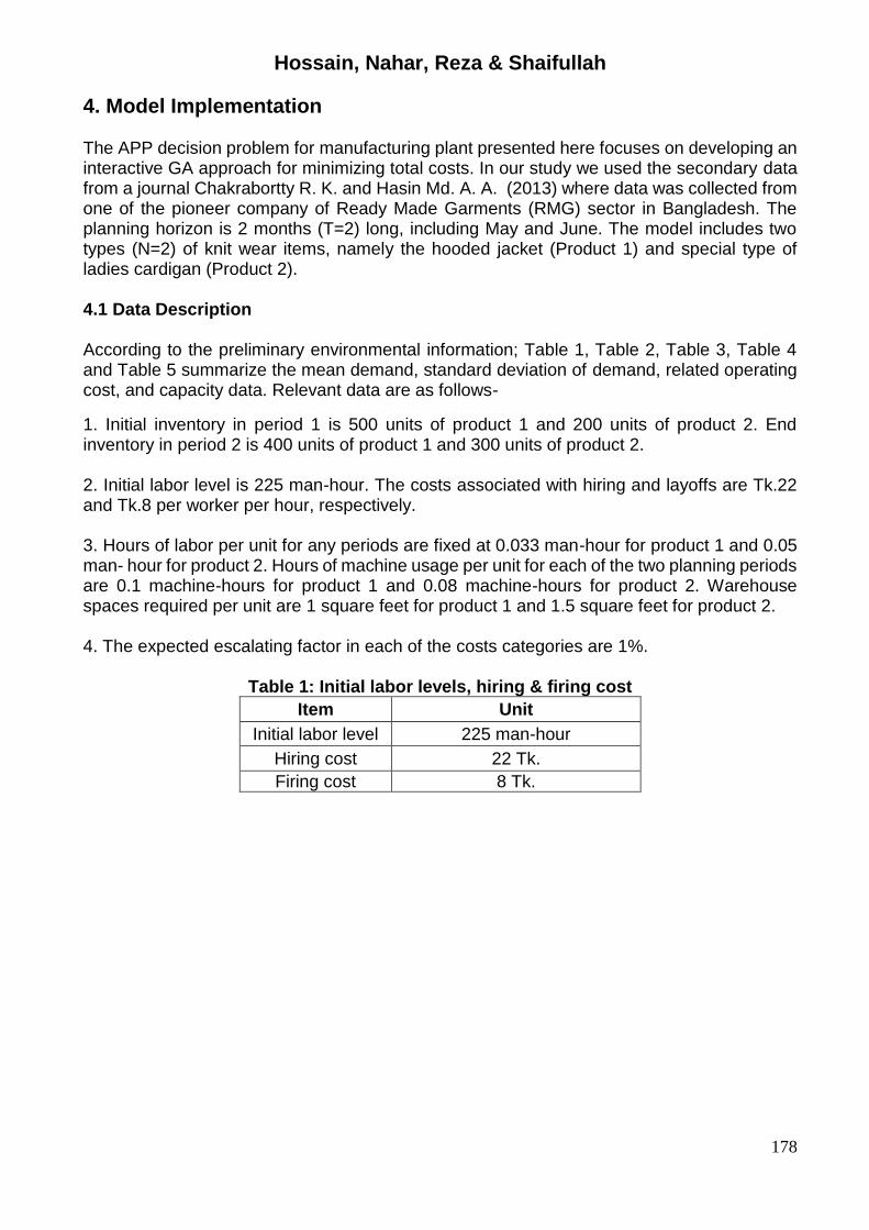
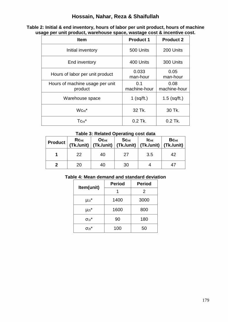
4. Model Implementation The APP decision problem for manufacturing plant presented here focuses on developing an interactive GA approach for minimizing total costs. In our study we used the secondary data from a journal Chakrabortty R. K. and Hasin Md. A. A. (2013) where data was collected from one of the pioneer company of Ready Made Garments (RMG) sector in Bangladesh. The planning horizon is 2 months (T=2) long, including May and June. The model includes two types (N=2) of knit wear items, namely the hooded jacket (Product 1) and special type of ladies cardigan (Product 2). 4.1 Data Description According to the preliminary environmental information; Table 1, Table 2, Table 3, Table 4 and Table 5 summarize the mean demand, standard deviation of demand, related operating cost, and capacity data. Relevant data are as follows-

1. Initial inventory in period 1 is 500 units of product 1 and 200 units of product 2. End inventory in period 2 is 400 units of product 1 and 300 units of product 2. 2. Initial labor level is 225 man-hour. The costs associated with hiring and layoffs are Tk.22 and Tk.8 per worker per hour, respectively. 3. Hours of labor per unit for any periods are fixed at 0.033 man-hour for product 1 and 0.05 man- hour for product 2. Hours of machine usage per unit for each of the two planning periods are 0.1 machine-hours for product 1 and 0.08 machine-hours for product 2. Warehouse spaces required per unit are 1 square feet for product 1 and 1.5 square feet for product 2. 4. The expected escalating factor in each of the costs categories are 1%.

Table 1: Initial labor levels, hiring & firing cost

Item Unit

Initial labor level 225 man-hour

Hiring cost 22 Tk.

Firing cost 8 Tk.


179

Table 2: Initial & end inventory, hours of labor per unit product, hours of machine usage per unit product, warehouse space, wastage cost & incentive cost.

Item Product 1 Product 2

Initial inventory 500 Units 200 Units

End inventory 400 Units 300 Units

Hours of labor per unit product 0.033

man-hour 0.05

man-hour

Hours of machine usage per unit product

0.1 machine-hour

0.08 machine-hour

Warehouse space 1 (sq/ft.) 1.5 (sq/ft.)

Wcnt* 32 Tk. 30 Tk.

Tcnt* 0.2 Tk. 0.2 Tk.

Table 3: Related Operating cost data

Product Rcnt

(Tk./unit)

Ocnt

(Tk./unit)

Scnt

(Tk./unit)

Icnt

(Tk./unit)

Bcnt

(Tk./unit)

1 22 40 27 3.5 42

2 20 40 30 4 47

Table 4: Mean demand and standard deviation

Item(unit) Period Period

1 2

µ1t* 1400 3000

µ2t* 1600 800

σ1t* 90 180

σ2t* 100 50


180

Table 5: Maximum labor, machine, warehouse capacity, back order level, subcontracted volume & minimum Inventory data, allowable wastage, targeted

production Period Period Period Period

Item(unit) 1 2 Item(unit) 1 2

I1tmin 300 350 S1tmax 200 350

I2tmin 150 200 S2tmax 100 100

Tp1t* 1250 2800 B1tmax 60 150

Tp2t* 1450 700 B2tmax 50 40

Wtmax 1000 1000 Aw1t* 42 90

Ltmax 225 225 Aw2t* 48 24

Mtmax 400 500

* Data was collected from Comfit Composite Knit Limited (CCKL).

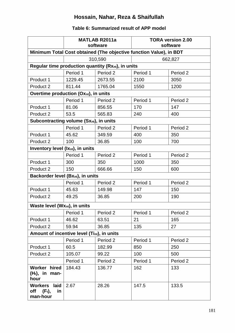
5. Result Analysis By using MATLAB R2011a software - Objective function value, which is obtained considering Genetic Algorithm (GA) optimization technique is BDT 310,590 and by using TORA version 2.00, Feb. 2006 software - Objective function value, which is obtained considering Big M method is BDT 662,827. Summarized result that are obtained by using Genetic Algorithm (GA) optimization technique in MATLAB R2011a and Big M method in TORA version 2.00, Feb. 2006 software are given in table 6.


181

Table 6: Summarized result of APP model

MATLAB R2011a software

TORA version 2.00 software

Minimum Total Cost obtained (The objective function Value), in BDT

310,590 662,827

Regular time production quantity (Rxnt), in units

Period 1 Period 2 Period 1 Period 2

Product 1 1229.45 2673.55 2100 3050

Product 2 811.44 1765.04 1550 1200

Overtime production (Oxnt), in units


Product 1 81.06 856.55 170 147

Product 2 53.5 565.83 240 400

Subcontracting volume (Sxnt), in units


Product 1 45.62 349.59 400 350

Product 2 100 36.85 100 700

Inventory level (Ixnt), in units


Product 1 300 350 1000 350

Product 2 150 666.66 150 600

Backorder level (Bxnt), in units


Product 1 45.63 149.98 147 150

Product 2 49.25 36.85 200 190

Waste level (Wxnt), in units


Product 1 46.62 63.51 21 165

Product 2 59.94 36.85 135 27

Amount of incentive level (Tint), in units


Product 1 60.5 182.99 850 250

Product 2 105.07 99.22 100 500


Worker hired (Ht), in man-hour

184.43 136.77 162 133

Workers laid off (Ft), in man-hour

2.67 28.26 147.5 133.5


182

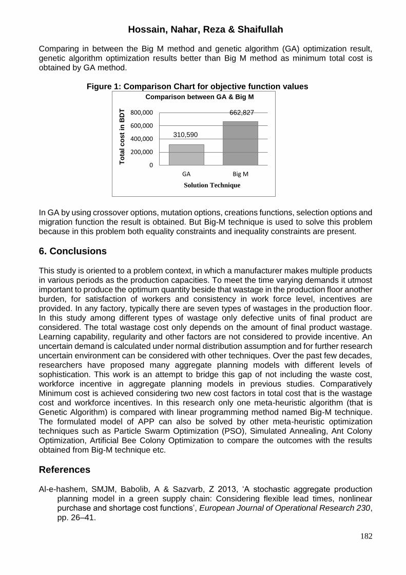
Comparing in between the Big M method and genetic algorithm (GA) optimization result, genetic algorithm optimization results better than Big M method as minimum total cost is obtained by GA method. Figure 1: Comparison Chart for objective function values

In GA by using crossover options, mutation options, creations functions, selection options and migration function the result is obtained. But Big-M technique is used to solve this problem because in this problem both equality constraints and inequality constraints are present.

6. Conclusions This study is oriented to a problem context, in which a manufacturer makes multiple products in various periods as the production capacities. To meet the time varying demands it utmost important to produce the optimum quantity beside that wastage in the production floor another burden, for satisfaction of workers and consistency in work force level, incentives are provided. In any factory, typically there are seven types of wastages in the production floor. In this study among different types of wastage only defective units of final product are considered. The total wastage cost only depends on the amount of final product wastage. Learning capability, regularity and other factors are not considered to provide incentive. An uncertain demand is calculated under normal distribution assumption and for further research uncertain environment can be considered with other techniques. Over the past few decades, researchers have proposed many aggregate planning models with different levels of sophistication. This work is an attempt to bridge this gap of not including the waste cost, workforce incentive in aggregate planning models in previous studies. Comparatively Minimum cost is achieved considering two new cost factors in total cost that is the wastage cost and workforce incentives. In this research only one meta-heuristic algorithm (that is Genetic Algorithm) is compared with linear programming method named Big-M technique. The formulated model of APP can also be solved by other meta-heuristic optimization techniques such as Particle Swarm Optimization (PSO), Simulated Annealing, Ant Colony Optimization, Artificial Bee Colony Optimization to compare the outcomes with the results obtained from Big-M technique etc.

References Al-e-hashem, SMJM, Babolib, A & Sazvarb, Z 2013, ‘A stochastic aggregate production

planning model in a green supply chain: Considering flexible lead times, nonlinear purchase and shortage cost functions’, European Journal of Operational Research 230, pp. 26–41.

310,590

662,827

0

200,000

400,000

600,000

800,000

GA Big M

To

tal co

st

in B

DT

Solution Technique

Comparison between GA & Big M


183

Aliev, RA, Fazlollahi, B, Guirimov, BG, & Aliev, RR 2007, ‘Fuzzy-genetic approach to aggregate production-distribution planning in supply chain management Information Sciences’, 177, pp. 4241–4255.

Andreas, AK & Smith, JC 2009, ‘Decomposition algorithms for the design of a no simultaneous capacitated evacuation tree network’, Networks, 52 2, pp. 91–103.

Ashayeri, J & Selen, W 2003, ‘A production planning model and a case study for the pharmaceutical industry in The Netherlands’, Journal of Logistics: Research and Applications; 61/2, pp. 37–50.

Baltas, Tsafarakis, Saridakis & Matsatsinis 2013, ‘Biologically inspired approaches to strategic service design: Optimal service diversification through evolutionary and swarm intelligence models’, Journal of Service Research, 16, pp. 186-201.

Baykasogluy, A 2006, ‘MOAPP.S 10: Aggregate production planning using the multiple objective tabu search’, International Journal of Production Research, 39 16, pp. 3685-3702.

Bish, DR, Sherali, HD & Hobeika, AG 2011b, Optimal Evacuation Strategies with Staging and Routing, Department of Industrial and Systems Engineering, Virginia Tech, Blacksburg, VA manuscript.

Bunnag, D & Sun, M 2005, ‘Genetic Algorithm for constrained global optimization in continuous variables’, Applied Mathematics and Computation, 171, pp. 604–636.

Chakrabortty, RK & Hasin, Md. AA 2013, ‘Solving an aggregate production planning problem by using multi-objective genetic algorithm MOGA approach’, International Journal of Industrial Engineering Computations, 4, pp. 1–12.

Chalmet, LG, Francis, RL & Saunders, PB 1982, ‘Quickest flows over time’, Management Science, 28 1, pp. 86–105.

Chiu, Y, Zheng, H, Villalobos, J & Gautam, B 2007, ‘Modeling no-notice mass evacuation using a dynamic traffic flow optimization model’, IIE Transactions, 39 1, pp. 83–94.

Disney, SM, Naim, MM & Potter, A 2004, ‘Assessing the impact of e-business on supply chain dynamics’, Int J Prod Econ, 89 2, pp. 109–118.

Dotoli, M, Fanti, MP, Meloni, C & Zhou, M 2006, ‘Design and optimization of integrated e-supply chain for agile and environmentally conscious manufacturing’, IEEE Trans Syst Man Cyb Part A: Syst Hum, 36 1, pp. 62–75.

Fahimnia, Luong & Marian 2006, ‘Modeling and optimization of aggregate production planning- A Genetic Algorithm’, Proceedings of World Academy of Science, Engineering and Technology.

Feng, P & Rakesh, N 2010, ‘Robust supply chain design under uncertain demand in agile manufacturing’, Computers & Operations Research, 37 4, pp. 668–683.

Ganesh, K & Punniyamoorthy, M 2005, ‘Optimization of continuous-time production planning using hybrid Genetic Algorithms- Simulated Annealing’, International Journal of Advance Manufacturing Technology, 26, pp. 148-154.

Gaonkar, R & Viswanadham, N 2005, ‘Strategic sourcing and collaborative planning in internet-enabled supply chain networks producing multi generation products’, IEEE Trans Autom Sci Eng, 2 1, pp. 54–66.

Jung, H & Jeong, B 2005, ‘Decentralized production-distribution planning system using collaborative agents in supply chain network’, Int J Adv Manuf Technol, Springer London, 25 1–2, pp. 167–173.

Ioannis, GT 2009, ‘Solving constrained optimization problems using a novel genetic algorithm’, Applied Mathematics and Computation, 208, pp. 273–283.

Jiang, Kong, & Li 2008, ‘Aggregate production planning model of production line in iron & steel enterprise based on Genetic Algorithm’, Proceedings of the 7th World Congress on Intelligent Control Automation, Chongqing, China.


184

Kazemi-Zanjani, M, Ait-Kadi, D & Nourelfath, M 2010, ‘Robust production planning in a manufacturing environment with random yield: a case in sawmill production planning’, European Journal of Operational Research, 201 3, pp. 882–891.

Liang, TF 2007, ‘Application of interactive possibilistic linear programming to aggregate production planning with multiple imprecise objectives’, Production Planning and Control, 187, pp. 548–560.

Kumar, MG, & Haq, NA 2005, ‘Hybrid genetic-ant colony algorithms for solving aggregate production plan’, Journal of Advanced Manufacturing Systems, JAMS, 1, pp. 103-111.

Ning, Y, Tang, W, & Zhao, R 2006, ‘Multi-product aggregate production planning in fuzzy random environments’, World Journal of Modeling and Simulation, 22, pp. 312–321.

Paiva & Morabito 2009, ‘An optimization model for aggregate production planning of a Brazilian sugar an ethanol milling company’, Annals of Operations Research, 169, pp. 117-130.

Pega, MF, Lisboa, JV & Yasin, M 2000, ‘The financial aspects of aggregate production planning: an application of time proven techniques’, International Journal of Commerce and Management, 103&4, pp. 35–42.

Pradenas, L, & Pe-nailillo, F 2004, ‘Aggregate production planning problem: A new algorithm’, Electronic Notes in Discrete Mathematics, 18, pp. 193-199.

Ramazanian and Modares 2011, ‘Application of particle swarm optimization algorithm to aggregate production planning’, Asian Journal of Business Management Studies, 2, pp. 44-54.

Ramezanian, R, Rahmani, D, & Barzinpour, F 2012, ‘An aggregate production planning model for two phase production systems: Solving with genetic algorithm and tabu search’, Expert Systems with Applications, 39, pp. 1256-1263.

Sharma, DK, & Jana RK 2009, ‘Fuzzy goal programming based genetic algorithm approach to nutrient management for rice crop planning’, International Journal of Production Economics, 121, pp. 224–232.

Silva, Figureria, Lisboa & Barman 2006, ‘An interactive decision support system for an aggregate production planning model based on multiple criteria mixed integer linear programming’, Omega-International Journal of Management Science, 34, pp. 167-177.

Wang, RC, & Liang, TF 2004, ‘Application of fuzzy multi-objective linear programming to aggregate production planning’, Computers & Industrial Engineering, 46, pp. 17–41.

Wu, D, Olson & DL 2008, ‘Supply chain risk, simulation, and vendor selection’, International Journal of Production Economics, 114 2, pp. 646–655.

Wu, D & Olson, DL 2009a, ‘Enterprise risk management: small business scorecard analysis’, Production Planning & Control, 120 4, pp. 362–369.

Wu, D, & Olson, DL 2009b, ‘Introduction to the special issue on ‘‘Optimizing Risk Management: Methods and Tools’, Human and Ecological Risk Assessment, 15 2, pp. 220–226.

Wu, D & Olson, DL 2010b, ‘Enterprise risk management: a DEA VaR approach in vendor selection’, International Journal of Production Research, 48 16, pp. 4919–4932.

Wu, D & Olson, DL, 2010a, ‘Enterprise risk management: coping with model risk in a large bank’, Journal of the Operational Research Society, 61 2, pp. 179–190.

Wu, D, Xie, K & Chen, G 2010, ‘A risk analysis model in concurrent engineering product development’, Risk Analysis, 30 9, pp. 1440–1453.

Park, YB 2005, ‘An integrated approach for production and distribution planning in supp.ly chain management’, Int J Prod Res, 43 6, pp. 1205–1224.

Yao, T, Mandala, SR & Chung, BD 2009, ‘Evacuation transportation planning under uncertainty: a robust optimization approach’, Networks and Spatial Economics, 9 2, pp. 171–189.


185

Yeh, WC, & Chuang, MC 2011, ‘Using multi-objective genetic algorithm for partner selection in green supply chain problems’, Expert Systems with Applications, 38, pp. 4244-4253.

multi-period, multi-product, aggregate production … review of business research vol. 6. no. 2....

Documents