Multi-Step Ahead Estimation of Time Series Models

Tucker McElroy1 and Marc Wildi2

U.S. Census Bureau and Institute of Data Analysis and Process Design

Abstract

We study the fitting of time series models via minimization of a multi-step ahead forecast error

criterion that is based on the asymptotic average of squared forecast errors. Our objective

function uses frequency domain concepts, but is formulated in the time domain, and allows

estimation of all linear processes (e.g., ARIMA and component ARIMA). By using an asymptotic

form of the forecast mean squared error, we obtain a well-defined nonlinear function of the

parameters that is provably minimized at the true parameter vector when the model is correctly

specified. We derive the statistical properties of the parameter estimates, and study their impact

on multi-step ahead forecasting. The method is illustrated through a forecasting exercise applied

to several time series.

1 Center for Statistical Research and Methodology, U.S. Census Bureau, 4600 Silver Hill Road,

Washington, D.C. 20233-91002 Institute of Data Analysis and Process Design

Keywords. ARIMA, Forecasting, Frequency Domain, Nonstationary, Signal Extraction.

Disclaimer This report is released to inform interested parties of research and to encourage

discussion. The views expressed on statistical issues are those of the authors and not necessarily

those of the U.S. Census Bureau.

1 Introduction

It is well-known that fitting models via the minimization of one-step ahead forecasting error is

equivalent to maximum likelihood estimation of the Gaussian likelihood for a stationary time series,

and thus provides efficient parameter estimation for correctly specified Gaussian time series models;

see Hannan and Deistler (1988), Dahlhaus and Wefelmeyer (1994), Taniguchi and Kakizawa (2000).

But in reality models are never correctly specified, and thus the maximum likelihood estimates

converge to so-called “pseudo-true” values under certain regularity conditions, and these pseudo-

true values minimize the Kullback-Leibler (KL) discrepancy between the specified model spectral

density and the true spectrum. This approach can be viewed as an attempt to minimize one-step

1

ahead forecast error for a given process utilizing a certain misspecified model. Given that for some

applications more interest focuses on forecasting performance at high leads, it is natural to consider

the following questions: can we fit time series models such that multi-step ahead forecasting error

is minimized? Is there an objective function analogous to KL, which generalizes it to the multi-step

ahead case? What are the statistical properties of the resulting parameter estimates? This paper

provides answers to some of these questions.

We present a Generalized Kullback-Leibler (GKL) measure – which is really a multi-step ver-

sion of KL – and demonstrate that this measure can be directly derived from a multi-step ahead

forecasting error criterion. This GKL can be used with very little programming effort to fit lin-

ear time series models; in this paper we focus on the univariate ARIMA class1 of models. The

resulting parameter estimates are consistent for the pseudo-true values (i.e., the minimizers of the

GKL discrepancy between model and truth) under standard conditions, and are also asymptotically

normal. When the model is correctly specified, these estimates are inefficient, i.e., they perform

worse than the classical one-step ahead estimates; we discuss the reasons for this below. However,

since GKL is derived from a multi-step ahead forecasting error criterion, it is reasonable to hope

that forecasts generated from such a model – at that particular lead – will perform better than

the classical forecasts. This reflects an application-driven modeling philosophy: both model spec-

ification and estimation should be oriented around a particular objective function associated with

the application. McElroy and Findley (2010) addresses the model specification problem from a

multi-step ahead forecasting perspective, and here we focus on the model estimation aspect.

The GKL can be used to investigate the behavior of multi-step pseudo-true values – the mini-

mizers of the discrepancy between truth and misspecified model – and is also the basis for actual

parameter estimates that generalize the (one-step ahead) quasi-maximum likelihood estimates asso-

ciated with the Whittle likelihood. We note in passing that Theorem 4.3.1 of Hannan and Deistler

(1988) provides a discussion of the equivalency of Gaussian likelihood and Whittle likelihood in the

case that the model is correctly specified; when mis-specified, the proper reference is Dahlhaus and

Wefelmeyer (1994).

Let us briefly discuss the econometric motivations for considering the multi-step ahead perspec-

tive. Since time series models in reality are always misspecified, the crucial thing is to find a model

that performs well according to the prescribed task of interest to the practitioner; using GKL as an

objective function means the practitioner is interested in a model that forecasts well at a particular

lead. In econometric business cycle analysis there is little interest in mere one-step ahead perfor-

mance of misspecified models, since the period of a typical cycle is 8 to 40 observations for quarterly

data. A model or collection of models that can forecast well at lead h for 8 ≤ h ≤ 40 is needed here.1Although for one-step ahead forecasting, the KL does not depend on unit root factors in the autoregressive

polynomial, i.e., the differencing polynomial, in the multi-step ahead case this object participates directly in the

GKL function.

2

Another application is in the field of seasonal adjustment, and more generally the area of real-time

signal extraction. All model-based asymmetric signal extraction filters rely implicitly or explicitly

on long-horizon forecasts generated from the same misspecified model; see Dagum (1980), Findley

et al. (1998), Wildi (2004), and McElroy (2008). Real-time – or concurrent – signal extraction is

discussed in Wildi (2004, 2008), where the nefarious impact of model mis-specification on long-term

forecasting performance and signal extraction is highlighted through numerous empirical studies.

This situation has ramifications for official seasonal adjustment procedures such as X-12-ARIMA2

and TRAMO-SEATS3. Beyond these obvious applications, any data analysis that is contingent

on long-run forecasts – such as occur in climatology (e.g., the hot topic of global warming) and

demographics (e.g., forecasting long-term changes in human population) – should not rely solely

upon one-step ahead forecasting model fitting criteria.

In light of these important motivations, there has been prior work on this topic that deserves

mention. The first thorough treatment that we are aware of is Gersch and Kitagawa (1983); they

estimate structural models using a heuristic 12-step ahead form of the usual Gaussian likelihood,

expressed in a state space form. This innovative paper illustrates the impact of a multi-step ahead

model fitting criterion on forecasting and trend estimation – as expected, the trends resulting from

the 12-step ahead criterion are much smoother than those derived from the classical approach. We

seek to go beyond this paper by providing an explicit discussion of asymptotic objective functions,

pseudo-true values, and statistical behavior of parameter estimates, while allowing for completely

generic linear models (our theoretical results apply to structural models such as those of Harvey

(1989), although our applications focus on simple unconstrained ARIMA models). Another inter-

esting contribution is Haywood and Tunnicliffe-Wilson (1997), which provides an explicit formula

for the objective function written in the frequency domain. A limitation of theirs is that the vari-

ables of the objective function do not in general correspond to ARMA parameters, as the paper

essentially fits an unusual parametrization of moving average models. Our work aims to address

the multi-step ahead model fitting problem within the familiar context of ARIMA models, such

that the variables of the objective function directly correspond to the ARIMA model parameters.

It is appropriate to outline the limitations of our approach. We do not consider multivariate

time series models here; although the forecast error filter in this context is known and in principle

could be used to generalize our GKL, the actual implementation of such is yet unsolved. However,

it seems a fruitful direction for future work. Secondly, our method only optimizes over one forecast

lead at a time – simultaneous optimization over many leads is not considered; a discussion of this2The seasonal adjustment software of the U.S. Census Bureau; see Findley et al. (1998) for a discussion of the

methodology. The signal extraction method uses nonparametric symmetric filters applied to the data, which is

forecast and backcast extended (implicitly) in order to obtain signal estimates at the sample boundary.3The seasonal adjustment software of the Bank of Spain; see Maravall and Caparello (2004) for discussion. Model-

based signal extraction filters are obtained from component models deduced via the method of canonical decomposi-

tion (Burman (1980), Hillmer and Tiao (1982)).

3

is provided in Section 2, where we discuss a composite forecasting rule. Finally, our methods

are implemented only for simple ARIMA models, where the gradient of the spectral density with

respect to the parameter vector has a particularly simple form.

This paper provides the development of asymptotic forecast mean squared error as a model

fitting criterion in Section 2. A key contribution is the practical formula for its computation. Sta-

tistical properties of this GKL function and its optima are discussed in Section 3. Our formulation

of the problem provides well-defined objective functions, that are optimized by the true parameters

when the model is correctly specified; otherwise, the parameter estimates converge to the GKL

pseudo-true values. Section 4 explores the GKL function through several illustrations, both ana-

lytically and numerically. Then in Section 5 we explore the discrepancy between empirical forecast

error and GKL through a chemical time series, and display results from a forecasting exercise in-

volving several time series. Here we take models that may be mis-specifications for the data, and

fit them according to a variety of forecast lead criteria, generating the resulting forecasts. The

multi-step out-of-sample forecasts are then computed and compared across model fitting criteria.

Section 6 provides our conclusions, and the Appendix contains proofs and implementation notes

for ARIMA models.

2 Forecasting as Model Fitting Criteria

In this section we formulate a discrepancy measure for model fitting, which generalizes the KL

discrepancy. This is derived from the asymptotic mean square multi-step ahead forecasting error

for that model. We utilize γk(f) for the lag k autocorrelation function (acf) corresponding to a

given spectral density f – with the convention that γk(f) = (2π)−1 ∫ π−π f(λ)eiλk dλ – and associated

Toeplitz covariance matrix Γ(f), whose jkth entry is simply γj−k(f). We also use the notation

< g > for any function g of frequency to denote (2π)−1 ∫ π−π g(λ) dλ.

We will speak of time series models in terms of their spectral densities, since we are primarily

concerned with the second-order behavior of difference stationary time series. It will be convenient

to restrict ourselves to the “linear class” of spectra L, consisting of functions f that can be written

as f(λ) = |Ψ(e−iλ)|2σ2 for some causal power series Ψ(z) =∑

j≥0 ψjzj . We will assume that this

is an invertible representation, so that 1/Ψ(z) is well-defined on the unit circle. Here ψ0 = 1, and

σ2 is the innovation variance of the associated time series, i.e., σ2 = exp< log f >. Then a linear

model is some subset F of L parametrized by a vector θ, and we may write F = fθ : θ ∈ Θ for a

parameter space Θ.

When σ2 is a parameter of the model, it does not depend upon the other components of θ, and

we can order things such that σ2 is the last component. If there are r +1 parameters in total, then

θr+1 = σ2, and we refer to the first r components by the notation [θ], which omits the innovation

variance. In this case we say that fθ is “separable.” Clearly, ∇[θ]σ2 = 0 for separable models; if

4

this gradient is nonzero, then σ2 is not a parameter of the model, but rather a function of the other

model parameters. Then we have [θ] = θ, for a total of r parameters; this case is referred to as a

non-separable model. For example, ARMA models are separable, but component ARMA models

are not. For a separable model, f[θ] can be defined via fθ/σ2, and clearly only depends on [θ]. In

the non-separable case we use the same definition, by a convenient abuse of notation.

As discussed in McElroy and Findley (2010), there exist simple formulas for the h-step ahead

forecast error from a given model applied to a semi-infinite sample of a process. We consider the

direct forecasting problem, as opposed to iterating one-step ahead forecasting filters as in Proietti

(2011); also see Stock and Watson (1999) and Marcellino, Stock, and Watson (2006). Suppose

that our data process Xt is differenced to stationarity with differencing operator δ(B), which has

all its roots on the unit circle, such that the resulting Wt = δ(B)Xt is mean zero and stationary.

Suppose that Wt follows a model fθ ∈ F , so that we can write fθ(λ) = |Ψ(e−iλ)|2σ2. Note that

each coefficient ψj potentially depends on each of the first r components of θ. Then the h-step

ahead forecast error filter is simply the rational filter [Ψ/δ]h−10 (B)/Ψ(B) – derived in McElroy and

Findley (2010) – where the square brackets denote the truncation of an infinite power series to

those coefficients lying between the lower and upper bounds. In other words, [Ψ/δ]h−10 (B) is given

by computing a (nonconvergent) power series Ψ(B)/δ(B), and taking only the first h terms.

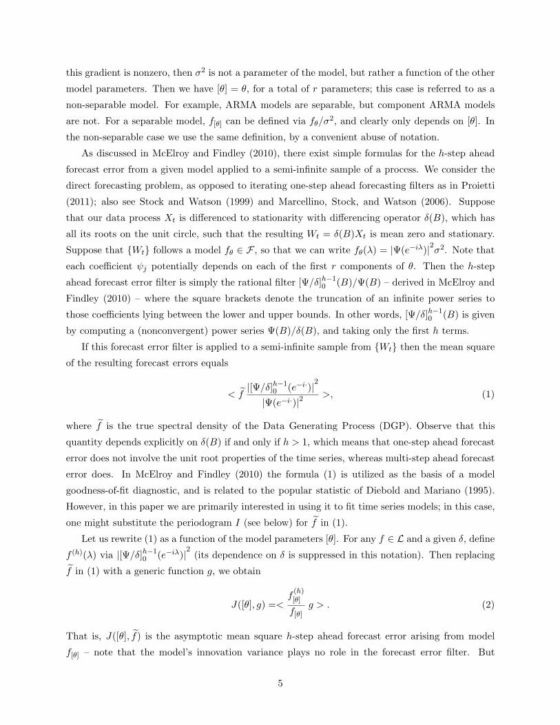
If this forecast error filter is applied to a semi-infinite sample from Wt then the mean square

of the resulting forecast errors equals

< f|[Ψ/δ]h−1

0 (e−i·)|2

|Ψ(e−i·)|2 >, (1)

where f is the true spectral density of the Data Generating Process (DGP). Observe that this

quantity depends explicitly on δ(B) if and only if h > 1, which means that one-step ahead forecast

error does not involve the unit root properties of the time series, whereas multi-step ahead forecast

error does. In McElroy and Findley (2010) the formula (1) is utilized as the basis of a model

goodness-of-fit diagnostic, and is related to the popular statistic of Diebold and Mariano (1995).

However, in this paper we are primarily interested in using it to fit time series models; in this case,

one might substitute the periodogram I (see below) for f in (1).

Let us rewrite (1) as a function of the model parameters [θ]. For any f ∈ L and a given δ, define

f (h)(λ) via |[Ψ/δ]h−10 (e−iλ)|2 (its dependence on δ is suppressed in this notation). Then replacing

f in (1) with a generic function g, we obtain

J([θ], g) =<f

(h)[θ]

f[θ]g > . (2)

That is, J([θ], f) is the asymptotic mean square h-step ahead forecast error arising from model

f[θ] – note that the model’s innovation variance plays no role in the forecast error filter. But

5

J([θ], I) is an empirical estimate of the mean squared error, where I(λ) = n−1|∑nt=1 Wte

−iλt|2 is

the periodogram computed on a sample of size n taken from the differenced series Wt.Now consider the minimization of J([θ], f) with respect to [θ] – the optimum [θ] yields a fitted

model f[θ]

with best possible forecast error within the model F . Likewise we can obtain an empirical

estimate via minimizing J([θ], I). Denote the optima of J via [θg], where g is alternatively I or f

depending on our interest. Consistency of [θI ] for [θf] will then follow from asymptotic results for

linear functionals of the periodogram (see Section 3 below).

With σ2 = exp< log f > we can write f = f[θf]σ

2 whenever the model is correctly specified.

Hence we can compute the true innovation variance from J via

σ2 =J([θ

f], f)

J([θf], f[θ

f])

.

This formula is trivial, but it does suggest an estimating equation by substituting I for f . More

generally, in terms of g we have

σ2g =

J ([θg], g)J

([θg], f[θg ]

) . (3)

Hence σ2I will be consistent for σ2, as shown in Section 3 below. Note that setting g = f in (3)

affords an interpretation for the pseudo-true value of the innovation variance, i.e., σ2f. Namely, it is

equal to the h-step ahead forecast MSE J([θf], f) arising from using the specified model, divided by

the normalization factor J([θf], f[θ

f]). When h = 1 this latter term equals unity, and plays no role,

but when h > 1 it modifies the simpler (and fallacious) interpretation of the innovation variance

as the h-step ahead forecast MSE. As a result, we have no reason to expect σ2f

to be increasing in

h, even though the h-step ahead forecast MSE is indeed typically increasing in h.

So these equations together give us an algorithm: first optimize (2) with respect to [θ], and

then compute the optimal σ2 via (3). When g = f , this provides us with the so-called pseudo-

true values (which in turn are h-step generalizations of the classical pseudo-true values of the KL

discrepancy, cf. Taniguchi and Kakizawa (2000)), and these are equal to the true parameters when

the model is correctly specified. But when g = I, this method provides us with parameter estimates

([θI ], σ2I ) that are consistent for the pseudo-true values (no matter whether the model is correctly

or incorrectly specified).

We now make some further connections of J with the KL discrepancy. It is well-known that

the log Gaussian likelihood for the differenced data Wt is approximately −1/2 times the Whittle

likelihood (Taniguchi and Kakizawa, 2000), which is simply the KL discrepancy between the peri-

odogram I and the model fθ. This KL discrepancy can be computed for any two positive bounded

functions f, g via the formula

KL(f, g) =< log f + g/f > . (4)

6

If we wish to fit a model to the data, we minimize KL(fθ, I) with respect to θ, denoting the resulting

estimate by θI . This can be done in two steps when fθ is separable, since then the KL is rewritten as

log σ2 + σ−2 < I/f[θ] so that the optimal σ2I equals < I/f[θI ] > (this requires ∇[θ]σ

2 = 0). In other

words, when the model is separable optimization of KL is equivalent to the two-step optimization

of (2) and (3) for h = 1.

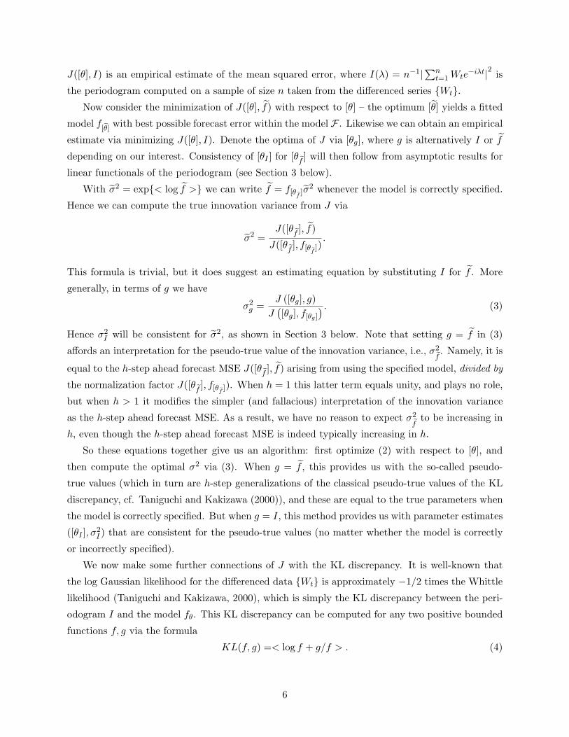
So Generalized Kullback-Leibler (GKL) discrepancy is defined analogously for h ≥ 1:

GKL(h)δ (f, g) =< log f > + log < f (h) > +

< gf f (h) >

< f (h) >. (5)

Note that this reduces to (4) when h = 1, since then f (h) ≡ 1. But for h > 1 we have the extra

log < f (h) > term, without which minimization of (5) would not be equivalent to optimization via

(2) and (3). This relationship is described in Proposition 2 of Section 3.

In practice, we can utilize the identities < g >= γ0(g) and < fI >= n−1W ′Γ(f)W to compute

GKL(h)δ (fθ, I), where W = (W1,W2, · · · ,Wn)′ is the available sample. Thus

GKL(h)δ (fθ, I) = log

(σ2γ0(f

(h)[θ] )

)+

W ′Γ(f

(h)[θ] /f[θ]

)W

nσ2γ0(f(h)[θ] )

. (6)

This is quite easy computationally for ARIMA models, for which the autocovariances are readily

obtained. The pseudo-true values, i.e., the values to which parameter estimates converge, are given

by the minimizers (when they exist) of GKL(h)δ (fθ, f). The statistical properties of the parameter

estimates is treated in the Section 3.

Thus, formula (6) gives a simple method for fitting models to time series data W , which gen-

eralizes Whittle estimation from h = 1 to h > 1. If this procedure is repeated over a range of h,

say 1 ≤ h ≤ H for some user-defined forecast threshold H, we obtain many different fits of the

specified model, with each corresponding parameter estimate θ(h) yielding optimal h-step ahead

(asymptotic) mean square forecast error. Of course, these parameters will vary widely in practice,

since there is no need that optimality be achieved over a range of forecast leads for one single

choice of parameters; this is illustrated in the numerical studies of Section 4. Having multiple fitted

models available is useful, since each fit is optimal with respect to its own h-step ahead forecasting

objective4.

Hence a strategy for optimal multi-step ahead forecasting is the following. For each h desired,

utilize the forecast filters based on the model fitted according to the GKL(h) criterion. Over

repeated forecasts, in an average sense, this procedure should prove to be advantageous (in-sample

this is necessarily so). We refer to this process as the composite forecasting rule. It is explored

further in Section 5 on a real time series.4The first author thanks Donald Gaver for this insightful perspective.

7

3 Statistical Properties of the Estimates

In this section we develop the statistical properties of GKL. First we present gradient and Hessian

expressions for the separable and non-separable cases. Optimization of GKL can then be easily

related to optimization of multi-step ahead forecasting error J . Then we state consistency and

asymptotic normality results for the parameter estimates under standard regularity conditions.

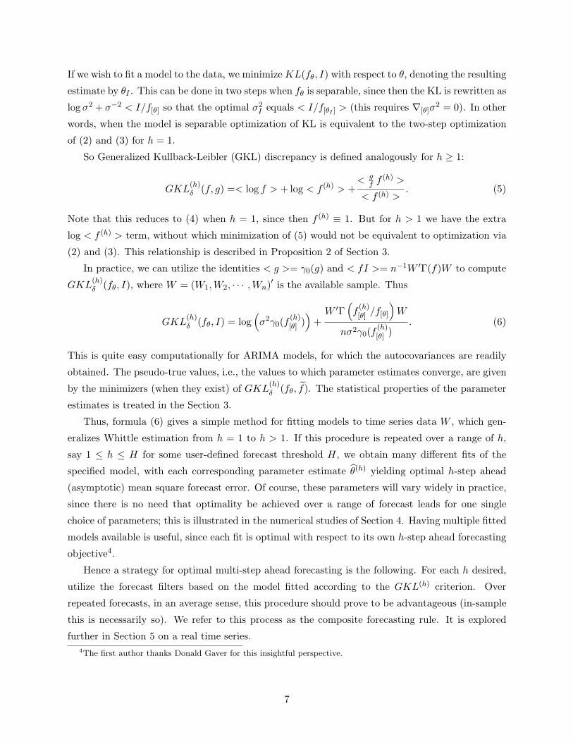
We begin by studying GKL(h)δ (fθ, g) as a function of θ, abbreviated as G(θ). It follows from

the definition (5) that

G(θ) = log σ2 + log < f(h)[θ] > +

J([θ], g)

σ2 < f(h)[θ] >

. (7)

Note that σ2 may well depend upon [θ] in the non-separable case, but this dependency will be

suppressed in the notation. Now (7) is convenient because it involves the function J . We begin

our treatment by noting that J([θ], f) has a global minimum at [θf] when the model is correctly

specified – this follows from MSE optimality of the h-step ahead forecast filter. In this case, f ∈ Fand there exists θ such that f = f

θ, so that [θ

f] = [θ] when the minimum is unique.

We next state the gradient and Hessian functions of G for the separable and non-separable

cases. In the former case, ∇′θ = [∇′[θ], ∂∂σ2 ], whereas in the latter case we have ∇θ = ∇[θ], since

there is no differentiation with respect to innovation variance (σ2 is not a parameter).

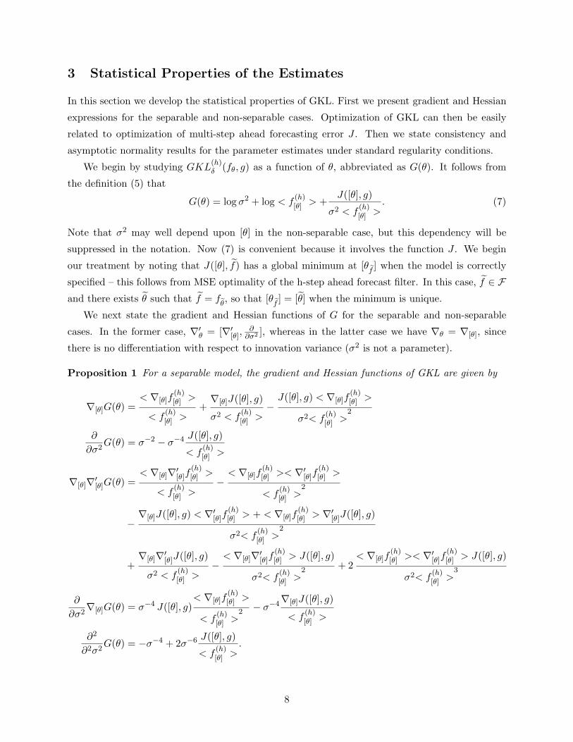
Proposition 1 For a separable model, the gradient and Hessian functions of GKL are given by

∇[θ]G(θ) =< ∇[θ]f

(h)[θ] >

< f(h)[θ] >

+∇[θ]J([θ], g)

σ2 < f(h)[θ] >

−J([θ], g) < ∇[θ]f

(h)[θ] >

σ2< f(h)[θ] >

2

∂

∂σ2G(θ) = σ−2 − σ−4 J([θ], g)

< f(h)[θ] >

∇[θ]∇′[θ]G(θ) =< ∇[θ]∇′[θ]f

(h)[θ] >

< f(h)[θ] >

−< ∇[θ]f

(h)[θ] >< ∇′[θ]f

(h)[θ] >

< f(h)[θ] >

2

−∇[θ]J([θ], g) < ∇′[θ]f

(h)[θ] > + < ∇[θ]f

(h)[θ] > ∇′[θ]J([θ], g)

σ2< f(h)[θ] >

2

+∇[θ]∇′[θ]J([θ], g)

σ2 < f(h)[θ] >

−< ∇[θ]∇′[θ]f

(h)[θ] > J([θ], g)

σ2< f(h)[θ] >

2 + 2< ∇[θ]f

(h)[θ] >< ∇′[θ]f

(h)[θ] > J([θ], g)

σ2< f(h)[θ] >

3

∂

∂σ2∇[θ]G(θ) = σ−4 J([θ], g)

< ∇[θ]f(h)[θ] >

< f(h)[θ] >

2 − σ−4∇[θ]J([θ], g)

< f(h)[θ] >

∂2

∂2σ2G(θ) = −σ−4 + 2σ−6 J([θ], g)

< f(h)[θ] >

.

8

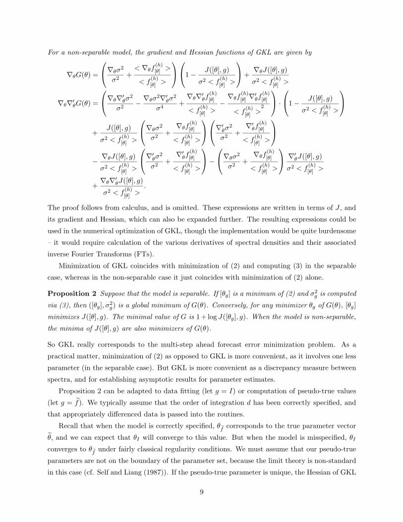
For a non-separable model, the gradient and Hessian functions of GKL are given by

∇θG(θ) =

∇θσ

2

σ2+

< ∇θf(h)[θ] >

< f(h)[θ] >

1− J([θ], g)

σ2 < f(h)[θ] >

+

∇θJ([θ], g)

σ2 < f(h)[θ] >

∇θ∇′θG(θ) =

∇θ∇′θσ2

σ2− ∇θσ

2∇′θσ2

σ4+∇θ∇′θf (h)

[θ]

< f(h)[θ] >

−∇θf

(h)[θ] ∇′θf

(h)[θ]

< f(h)[θ] >

2

·

1− J([θ], g)

σ2 < f(h)[θ] >

+J([θ], g)

σ2 < f(h)[θ] >

∇θσ

2

σ2+

∇θf(h)[θ]

< f(h)[θ] >

∇′θσ2

σ2+

∇′θf (h)[θ]

< f(h)[θ] >

− ∇θJ([θ], g)

σ2 < f(h)[θ] >

∇′θσ2

σ2+

∇′θf (h)[θ]

< f(h)[θ] >

−

∇θσ

2

σ2+

∇θf(h)[θ]

< f(h)[θ] >

∇′θJ([θ], g)

σ2 < f(h)[θ] >

+∇θ∇′θJ([θ], g)

σ2 < f(h)[θ] >

.

The proof follows from calculus, and is omitted. These expressions are written in terms of J , and

its gradient and Hessian, which can also be expanded further. The resulting expressions could be

used in the numerical optimization of GKL, though the implementation would be quite burdensome

– it would require calculation of the various derivatives of spectral densities and their associated

inverse Fourier Transforms (FTs).

Minimization of GKL coincides with minimization of (2) and computing (3) in the separable

case, whereas in the non-separable case it just coincides with minimization of (2) alone.

Proposition 2 Suppose that the model is separable. If [θg] is a minimum of (2) and σ2g is computed

via (3), then ([θg], σ2g) is a global minimum of G(θ). Conversely, for any minimizer θg of G(θ), [θg]

minimizes J([θ], g). The minimal value of G is 1+ log J([θg], g). When the model is non-separable,

the minima of J([θ], g) are also minimizers of G(θ).

So GKL really corresponds to the multi-step ahead forecast error minimization problem. As a

practical matter, minimization of (2) as opposed to GKL is more convenient, as it involves one less

parameter (in the separable case). But GKL is more convenient as a discrepancy measure between

spectra, and for establishing asymptotic results for parameter estimates.

Proposition 2 can be adapted to data fitting (let g = I) or computation of pseudo-true values

(let g = f). We typically assume that the order of integration d has been correctly specified, and

that appropriately differenced data is passed into the routines.

Recall that when the model is correctly specified, θf

corresponds to the true parameter vector

θ, and we can expect that θI will converge to this value. But when the model is misspecified, θI

converges to θf

under fairly classical regularity conditions. We must assume that our pseudo-true

parameters are not on the boundary of the parameter set, because the limit theory is non-standard

in this case (cf. Self and Liang (1987)). If the pseudo-true parameter is unique, the Hessian of GKL

9

should be positive definite at that value, and hence invertible. The so-called Hosoya-Taniguchi (HT)

conditions (Hosoya and Taniguchi (1982) and Taniguchi and Kakizawa (2000)) impose sufficient

regularity on the process Wt to ensure a central limit theorem; these conditions require that

the process is a causal filter of a higher-order martingale difference. Finally, we suppose that the

fourth order cumulant function of the process is identically zero, which says that in terms of second

and fourth order structure the process looks Gaussian. This condition is not strictly necessary,

but facilitates a simple expression for the asymptotic variance of the parameter estimates. Let the

Hessian of G(θ) with g = f be denoted H(θ).

Theorem 1 Suppose that θf

exists uniquely in the interior of Θ and that H(θf) is invertible.

Suppose that the process Wt has finite fourth moments, conditions (HT1)-(HT6) of Taniguchi

and Kakizawa (2000, pp.55-56) hold, and that the fourth order cumulant function of Wt is zero.

Then as n →∞ √n

(θI − θ

f

) L=⇒ N(0,H−1(θ

f)V (θ

f)H−1(θ

f))

. (8)

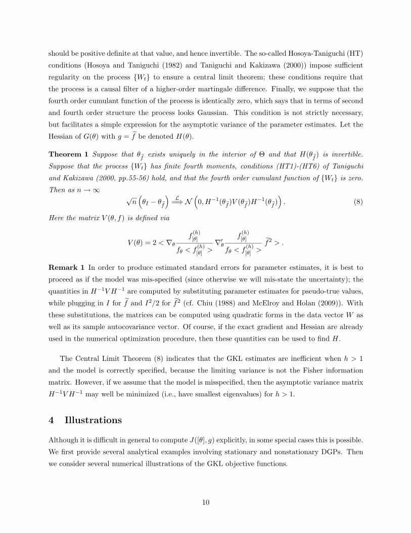
Here the matrix V (θ, f) is defined via

V (θ) = 2 < ∇θ

f(h)[θ]

fθ < f(h)[θ] >

∇′θf

(h)[θ]

fθ < f(h)[θ] >

f2 > .

Remark 1 In order to produce estimated standard errors for parameter estimates, it is best to

proceed as if the model was mis-specified (since otherwise we will mis-state the uncertainty); the

quantities in H−1V H−1 are computed by substituting parameter estimates for pseudo-true values,

while plugging in I for f and I2/2 for f2 (cf. Chiu (1988) and McElroy and Holan (2009)). With

these substitutions, the matrices can be computed using quadratic forms in the data vector W as

well as its sample autocovariance vector. Of course, if the exact gradient and Hessian are already

used in the numerical optimization procedure, then these quantities can be used to find H.

The Central Limit Theorem (8) indicates that the GKL estimates are inefficient when h > 1

and the model is correctly specified, because the limiting variance is not the Fisher information

matrix. However, if we assume that the model is misspecified, then the asymptotic variance matrix

H−1V H−1 may well be minimized (i.e., have smallest eigenvalues) for h > 1.

4 Illustrations

Although it is difficult in general to compute J([θ], g) explicitly, in some special cases this is possible.

We first provide several analytical examples involving stationary and nonstationary DGPs. Then

we consider several numerical illustrations of the GKL objective functions.

10

4.1 Analytical Derivations of Optima

When forecasting stationary processes long-term, forecasts tend to revert to the mean independent

of the parameter values (this can also be seen in the large h behavior of GKL when δ(z) = 1), and as

a result the objective function will be flat on the majority of its domain, i.e., changes in parameter

values have no impact on forecasting performance. This situation is dramatically different in the

presence of non-stationarity, because the large h behavior of GKL instead tends to infinity, rather

than a constant. Our results below are computed in terms of generic g, which can be taken as

either I or f as context dictates.

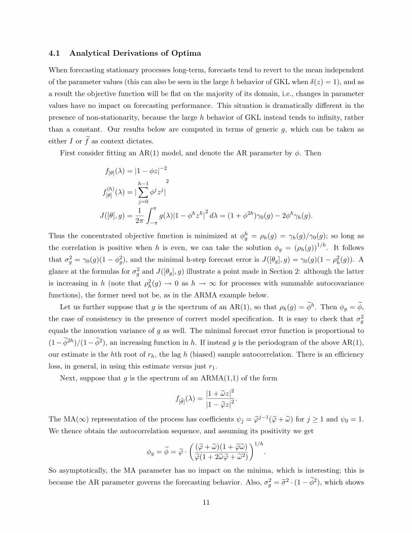
First consider fitting an AR(1) model, and denote the AR parameter by φ. Then

f[θ](λ) = |1− φz|−2

f(h)[θ] (λ) = |

h−1∑

j=0

φjzj |2

J([θ], g) =12π

∫ π

−πg(λ)|1− φhzh|2 dλ = (1 + φ2h)γ0(g)− 2φhγh(g).

Thus the concentrated objective function is minimized at φhg = ρh(g) = γh(g)/γ0(g); so long as

the correlation is positive when h is even, we can take the solution φg = (ρh(g))1/h. It follows

that σ2g = γ0(g)(1 − φ2

g), and the minimal h-step forecast error is J([θg], g) = γ0(g)(1 − ρ2h(g)). A

glance at the formulas for σ2g and J([θg], g) illustrate a point made in Section 2: although the latter

is increasing in h (note that ρ2h(g) → 0 as h → ∞ for processes with summable autocovariance

functions), the former need not be, as in the ARMA example below.

Let us further suppose that g is the spectrum of an AR(1), so that ρh(g) = φh. Then φg = φ,

the case of consistency in the presence of correct model specification. It is easy to check that σ2g

equals the innovation variance of g as well. The minimal forecast error function is proportional to

(1− φ2h)/(1− φ2), an increasing function in h. If instead g is the periodogram of the above AR(1),

our estimate is the hth root of rh, the lag h (biased) sample autocorrelation. There is an efficiency

loss, in general, in using this estimate versus just r1.

Next, suppose that g is the spectrum of an ARMA(1,1) of the form

f[θ]

(λ) =|1 + ωz|2|1− ϕz|2 .

The MA(∞) representation of the process has coefficients ψj = ϕj−1(ϕ + ω) for j ≥ 1 and ψ0 = 1.

We thence obtain the autocorrelation sequence, and assuming its positivity we get

φg = φ = ϕ ·(

(ϕ + ω)(1 + ϕω)ϕ(1 + 2ωϕ + ω2)

)1/h

.

So asymptotically, the MA parameter has no impact on the minima, which is interesting; this is

because the AR parameter governs the forecasting behavior. Also, σ2g = σ2 · (1− φ2), which shows

11

that the pseudo-true value of the innovation variance is less than the actual true σ2. Moreover, φ

is an increasing function of h, so that σ2g is decreasing in h.

Finally, suppose the process is a gap AR(2) with spectrum

f[θ]

(λ) = |1− ϕz2|−2.

The autocorrelations are zero at odd lags, and equal to ϕh/2 when the lag h is even. Supposing

ϕ > 0, we obtain φg = φ =√

ϕ for h even and zero otherwise. The corresponding innovation

variance is (1 + φ)−1

for h even and (1− ϕ2)−1 for h odd.

Now suppose that we fit an MA(q) model, which has spectral density

f[θ](λ) = |1 +q∑

j=1

ωjzj |

2

.

The resulting expression for J is fairly complicated in general, but when h > q we have f(h)[θ] = f[θ],

so that J([θ], g) = γ0(g). Thus the concentrated objective function is completely flat with respect

to the parameters, and model estimation is impossible. This reflects the fact that an MA(q) model

has no serial information by which to forecast at leads exceeding q. However, the problem is no

longer present when non-stationary differencing is present.

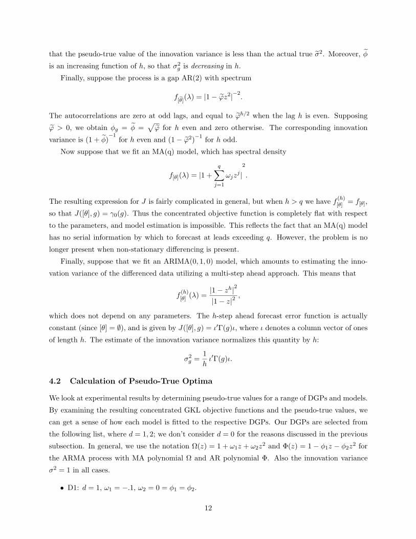
Finally, suppose that we fit an ARIMA(0, 1, 0) model, which amounts to estimating the inno-

vation variance of the differenced data utilizing a multi-step ahead approach. This means that

f(h)[θ] (λ) =

|1− zh|2|1− z|2 ,

which does not depend on any parameters. The h-step ahead forecast error function is actually

constant (since [θ] = ∅), and is given by J([θ], g) = ι′Γ(g)ι, where ι denotes a column vector of ones

of length h. The estimate of the innovation variance normalizes this quantity by h:

σ2g =

1h

ι′Γ(g)ι.

4.2 Calculation of Pseudo-True Optima

We look at experimental results by determining pseudo-true values for a range of DGPs and models.

By examining the resulting concentrated GKL objective functions and the pseudo-true values, we

can get a sense of how each model is fitted to the respective DGPs. Our DGPs are selected from

the following list, where d = 1, 2; we don’t consider d = 0 for the reasons discussed in the previous

subsection. In general, we use the notation Ω(z) = 1 + ω1z + ω2z2 and Φ(z) = 1− φ1z − φ2z

2 for

the ARMA process with MA polynomial Ω and AR polynomial Φ. Also the innovation variance

σ2 = 1 in all cases.

• D1: d = 1, ω1 = −.1, ω2 = 0 = φ1 = φ2.

12

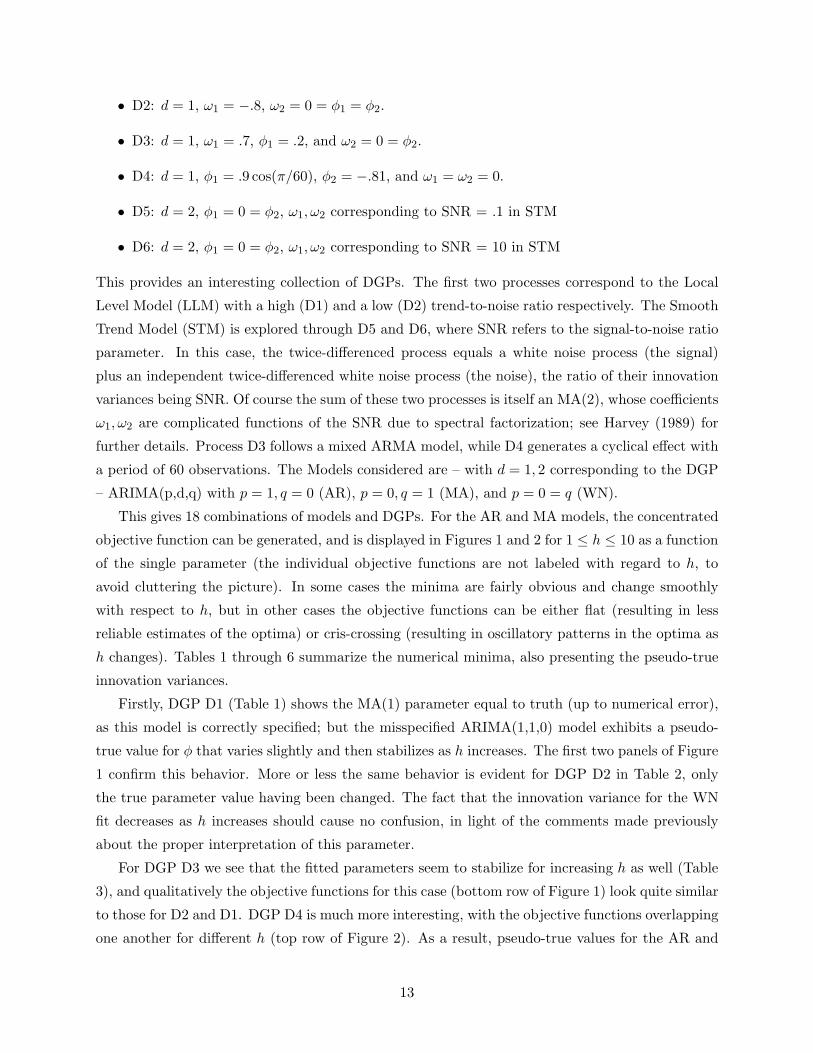
• D2: d = 1, ω1 = −.8, ω2 = 0 = φ1 = φ2.

• D3: d = 1, ω1 = .7, φ1 = .2, and ω2 = 0 = φ2.

• D4: d = 1, φ1 = .9 cos(π/60), φ2 = −.81, and ω1 = ω2 = 0.

• D5: d = 2, φ1 = 0 = φ2, ω1, ω2 corresponding to SNR = .1 in STM

• D6: d = 2, φ1 = 0 = φ2, ω1, ω2 corresponding to SNR = 10 in STM

This provides an interesting collection of DGPs. The first two processes correspond to the Local

Level Model (LLM) with a high (D1) and a low (D2) trend-to-noise ratio respectively. The Smooth

Trend Model (STM) is explored through D5 and D6, where SNR refers to the signal-to-noise ratio

parameter. In this case, the twice-differenced process equals a white noise process (the signal)

plus an independent twice-differenced white noise process (the noise), the ratio of their innovation

variances being SNR. Of course the sum of these two processes is itself an MA(2), whose coefficients

ω1, ω2 are complicated functions of the SNR due to spectral factorization; see Harvey (1989) for

further details. Process D3 follows a mixed ARMA model, while D4 generates a cyclical effect with

a period of 60 observations. The Models considered are – with d = 1, 2 corresponding to the DGP

– ARIMA(p,d,q) with p = 1, q = 0 (AR), p = 0, q = 1 (MA), and p = 0 = q (WN).

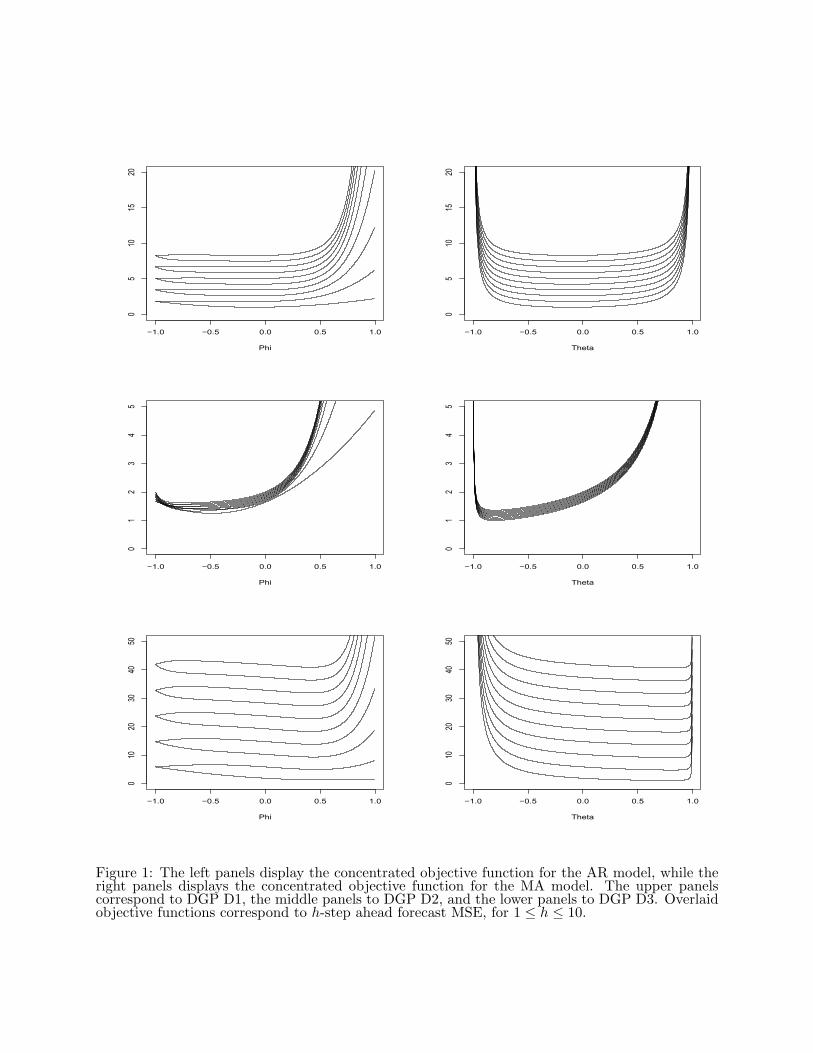
This gives 18 combinations of models and DGPs. For the AR and MA models, the concentrated

objective function can be generated, and is displayed in Figures 1 and 2 for 1 ≤ h ≤ 10 as a function

of the single parameter (the individual objective functions are not labeled with regard to h, to

avoid cluttering the picture). In some cases the minima are fairly obvious and change smoothly

with respect to h, but in other cases the objective functions can be either flat (resulting in less

reliable estimates of the optima) or cris-crossing (resulting in oscillatory patterns in the optima as

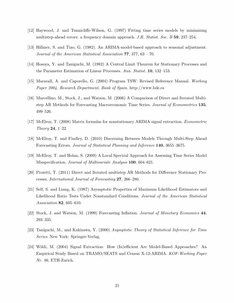
h changes). Tables 1 through 6 summarize the numerical minima, also presenting the pseudo-true

innovation variances.

Firstly, DGP D1 (Table 1) shows the MA(1) parameter equal to truth (up to numerical error),

as this model is correctly specified; but the misspecified ARIMA(1,1,0) model exhibits a pseudo-

true value for φ that varies slightly and then stabilizes as h increases. The first two panels of Figure

1 confirm this behavior. More or less the same behavior is evident for DGP D2 in Table 2, only

the true parameter value having been changed. The fact that the innovation variance for the WN

fit decreases as h increases should cause no confusion, in light of the comments made previously

about the proper interpretation of this parameter.

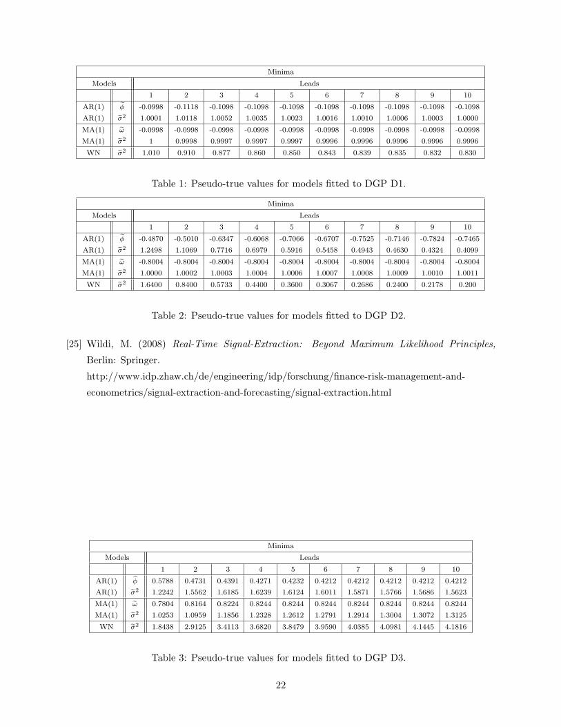
For DGP D3 we see that the fitted parameters seem to stabilize for increasing h as well (Table

3), and qualitatively the objective functions for this case (bottom row of Figure 1) look quite similar

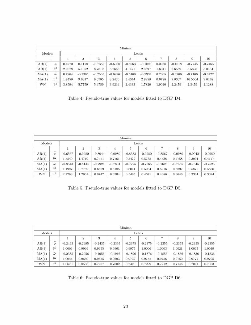
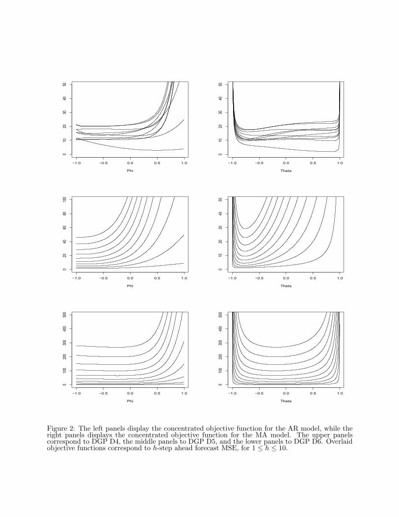
to those for D2 and D1. DGP D4 is much more interesting, with the objective functions overlapping

one another for different h (top row of Figure 2). As a result, pseudo-true values for the AR and

13

MA parameters change quite a bit, and seem not to stabilize in h (Table 4). This is no surprise,

given the strong spectral peak in the data process that is ill-captured by the grossly misspecified

models. As h increases, a different snap-shot of this cyclical process is obtained, and the h-step

ahead forecast error is optimized accordingly.

Finally, we have DGPs D5 and D6 (Tables 5 and 6), which exhibit distinct behavior in the

objective functions from the other cases (middle and bottom rows of Figure 2). Unfortunately,

portions of these likelihoods (especially in the AR model case) are extremely flat, resulting in

numerical imprecisions in the statement of the optima. The ARIMA(0,2,1) performs slightly better,

since in a sense it is less badly misspecified, the true model being an ARIMA(0,2,2). Also, the

increased SNR in D6 makes the trend in the STM more dominant, which presumably facilitates

forecasting (as compared to a noisier process), and this may be the reason that the optima are

better behaved.

5 Empirical Results

We first study a time series of chemical data from an in-sample forecasting perspective, in order

to show the correspondence between GKL, J , and empirical forecast error. Then we study several

seasonal time series originally featured in the NN3 forecasting competition5, with the interesting

finding that GKL with h = 12 performs competitively with the classical h = 1 criterion.

5.1 Chemical Data

We consider Chemical Process Concentration Readings (Chem for short)6. The sample has 197

observations. This data set was studied in McElroy and Findley (2010), where it was argued that

an ARIMA(0, 1, 1) model was most appropriate, given several contenders, according to multi-step

ahead forecasting criteria. Fitting Chem using GKL(h) yields the MA(1) polynomials 1 − .7B,

1− .8B, and 1− .84B for h = 1, 2, 3 respectively.

We noted earlier (Section 2) that J is an asymptotic form of the forecast mean squared error.

Empirical forecasts are generated from a finite sample of data, so that the actual forecast error

filter is an approximate truncation of [Ψ/δ]h−10 (B)/Ψ(B). As discussed in McElroy and Findley

(2010), J([θ], I) differs from the empirical forecast mean squared error by OP (n−1/2), where n is

the number of such forecasts.

So if we generate forecasts of Chem using a windowed sub-sample, and average the squared

forecast errors, the resulting behavior should mimic that of J as n increases. In particular, let

us consider the forecast h steps ahead, for h = 1, 2, 3, from a sample consisting of time indices

t = 1, 2, · · · , 197− n− h + s, repeated for s = 1, 2, · · · , n. Moreover, let us generate these forecasts5See http://www.neural-forecasting-competition.com/NN3/.6Available from http://www.stat.wisc.edu/ reinsel/bjr-data/index.html.

14

from each of the three GKL objective functions, for h = 1, 2, 3. Then the within-sample forecast

errors are calculated, squared, and averaged over s. The results can be summarized in a 3×3 table,

where the row j corresponds to the GKL(j) parameter used (so j = 1 corresponds to MA parameter

−.7, j = 2 corresponds to −.8, and j = 3 corresponds to −.84) and column k corresponds to the

forecast horizon. Note that the diagonal entries of the forecast error matrix correspond to forecasts

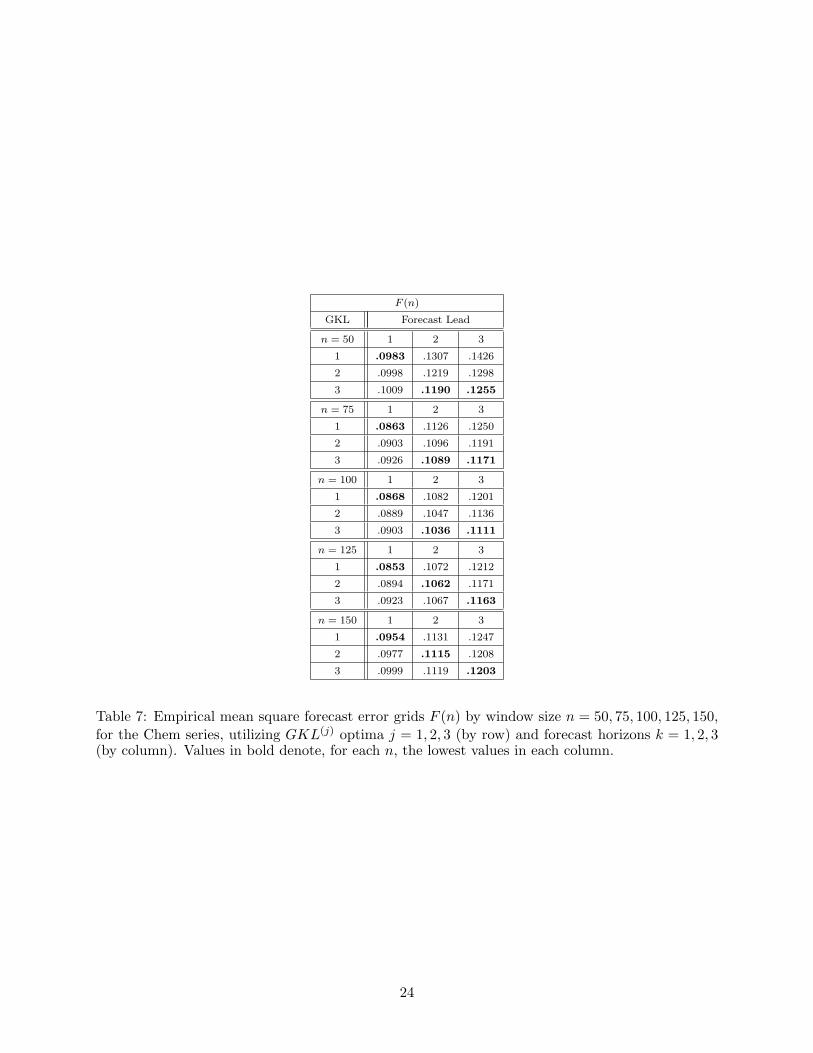
generated from the composite forecasting procedure described at the end of Section 2. Referring to

this forecast error matrix via F (n), we can expect the column minima to occur on the diagonals,

as n →∞. That is, minj Fjk(n) = Fkk(n) for each k = 1, 2, 3 for n large.

This is heuristic, because as we increase n we reduce the length of the forecast filters; neverthe-

less, Table 7 displays the pattern of F (n) for n = 50, 75, 100, 125, 150, and the expected property

holds starting at n = 125. It is also interesting that the 2-step GKL does well at 3-step ahead

forecasting for smaller n, in light of the close values (−.8 and −.84) for their respective MA pa-

rameters.

5.2 NN3 Data

Our goal here is to fit a common set of models to the various time series, generate out-of-sample

forecasts, and compare performance across the various GKL criteria utilized. A realistic assessment

of the composite forecasting rule, as was done for the Chem data, is not really possible for the NN3

Data due to the short length of the series (most of the series are seasonal with less than 12 years

in the sample, so that a windowing technique – such as was utilized with the Chem data – is not

compatible with having enough remaining data to get reasonable parameter estimates). Instead,

we examine a separate question: are there any NN3 series for which the forecasting performance “in

the competition” generated by a particular GKL(h) was superior to the classical forecasts arising

from GKL(1)? We describe the results of this query below.

The original NN3 competition utilized 111 monthly time series of varying lengths and starting

dates, for the most part exhibiting seasonal and trend dynamics, and from each a final span of 18

observations was with-held. We have obtained the full span of each time series from the contest’s

designers, so that we can assess performance.

In our study we attempt to mimic fairly closely the conditions of the competition, but restrict

to a common set of models to fix comparisons and facilitate didactic purposes. Therefore, we

used automatic SARIMA model identification software (X-12-ARIMA version 0.3) to determine

the Box-Cox transform, the preferred SARIMA model, and regression effects (outliers, trading day,

and Easter effects). Out of 111 series, 27 of them required a log transformation and were best

fitted by an Airline model, according to X-12-ARIMA. This was the largest subclass of identified

models, so we restricted our viewpoint to these 27 (this also includes some (010)(011) SARIMA

models, which of course are nested in the Airline model). Broadening our comparisons to include

15

other models would seem to cloud the picture – especially as plenty of series and models are

non-seasonal. We also work with the regression-adjusted series; this isolates the study to model

estimation, which seems reasonable given that fixed effects are very well understood.

So to each of the 27 regression-adjusted series, the last 18 observations were withheld, and the

log Airline model was fitted to the remaining data (so we could do the out-of-sample forecasting

exercise), using the GKL objective function with 1 ≤ h ≤ 18. The choice of leads was natural,

given the original competition was to forecast each series up to 18 periods ahead. For each of the 27

series, we computed an 18 by 18 grid of absolute forecast errors, with each column corresponding

to a forecast lead k and each row corresponding to a GKL(j) objective function. If we can sensibly

combine results across leads (along each row), then we obtain an overall assessment of each GKL(j)

as a forecasting procedure, for each of the 27 series.

The overall performance of submitted forecasts in the NN3 competition were judged according

to Symmetric Mean Absolute Percentage Error (SMAPE), which is described in Armstrong (1985),

so we adopt this as our method of synthesizing results. Letting Ak denote the target value (k steps

ahead) and Ak its forecast (from one of the GKL(j) forecasting methods), the formula is

SMAPE =118

18∑

k=1

2|Ak − Ak|Ak + Ak

.

These quantities were computed for each 1 ≤ j ≤ 18, and for all 27 series. The resulting values

are presented in Table 8. Also presented there is the best GKL(j) for each given series (i.e., the j

that yielded lowest SMAPE), as well as the ratio of its SMAPE to that of GKL(1). In some cases

there was substantial improvement over the h = 1 criterion – namely quasi-maximum likelihood

estimation – though results were variable over all. In the best cases, there was close to a 20 percent

improvement over classical estimation.

So if someone used a particular GKL(j) to produce all forecasts, and submitted the results to

the competition, which criteria would be successful relative to GKL(1) (for those 27 series)? The

two most successful such leads were j = 1 and j = 12, each of which performed best for 7 out

of the 27 series. Given the seasonal nature of these series, it is not surprising that 12-step ahead

forecasting is important to get right, and that a model optimized with respect to 12-step ahead

forecasting may perform well at shorter forecast leads too.

We examine this idea further with Series 110. In this case j = 12 was the overall winner, and

there is quite a bit of improvement over j = 1 – a 16 percent reduction to SMAPE. The parameters

for the latter case, i.e., the conventional estimates, were .08, .71 for the nonseasonal and seasonal

parameters of the Airline model. But when fitting with GKL(12), these became .99,−.25. This

is a radical, and meaningful, alteration to the parameters – from the long-term perspective, the

process is not really I(2), noting that the MA factor (1− .99B) can essentially be canceled with one

of the nonseasonal differencing operators of the model, reducing it to I(1) (once a compensating

16

mean regression effect is added). There is also a substantial change in the seasonal moving average

parameter. For this series, it seems likely that the airline model is a misspecification7 – it is in such

scenarios that our multi-step criterion can be expected to offer some improvements to forecasting

performance.

6 Conclusion

Classical model-based approaches typically emphasize a short-term one-step ahead forecasting per-

spective for estimating unknown model-parameters. This procedure could be justified by assuming

that the “true” model has been identified or that it is known a priori to the analyst. In contrast, we

here emphasize the importance of inferences based on multi-step ahead forecasting performances in

the practically more relevant context of misspecified models. For this purpose, we propose a gener-

alization of the well-known Kullback-Leibler discrepancy and we derive an asymptotic distribution

theory for estimates that converge to “pseudo-true” values. In contrast to earlier approaches, our

design is generic, i.e., it is not limited to a particular class of (linear) processes. We illustrate the

appeal of our approach by deriving closed-form solutions for a selection of simple processes. We

then compare performances of classical (one-step ahead) and generalized (h-step ahead) estimates

in a controlled experimental design based on a selection of simulated as well as practical time series.

Our empirical findings confirm the asymptotic theory, i.e., that the smallest forecast errors for a

given forecast lead arise from the corresponding criterion function for that lead (cf. the discussion

of the Chem series in Section 5.1). We find evidence in Series 110 that unit-root over-specification

(i.e., specifying a differencing operator of too high an order) can be mitigated, to some extent,

by longer-term forecasting criteria. Specifically, we found that for h = 12 one of the MA roots

approaches the unit circle, resulting in near cancelation of misspecified AR-roots.

In this paper we focused on univariate multi-step ahead forecasting over one forecast lead

at a time. As an outlook, we are interested in addressing more complex forecasting problems

such as simultaneous optimization over many leads or real-time signal extraction (computation of

concurrent trend or seasonal-adjustment filters) in univariate and multivariate frameworks. We

expect the frequency-domain approach underlying GKL to offer some promising perspectives on

these future topics.7The software X-12-ARIMA identifies a SARIMA model by inserting a dubious level shift regressor, whereas the

raw data shows little evidence of dynamic seasonality in its autocorrelation plot.

17

Appendix

A.1 Proofs

Proof of Proposition 2. Plugging [θ] = [θg] and σ2 = σ2g (3) into the gradient formulas in the

separable case of Proposition 1 shows that θg is a critical point of GKL, since ∇[θ]J([θ], g) evaluated

at [θ] = [θg] equals zero. Plugging into the Hessian formula yields, after simplification:

∇[θ]∇′[θ]G(θ)|θ=θg =∇[θ]∇′[θ]J([θ], g)|θ=θg

J([θg], g)+

< ∇[θ]f(h)[θ] >< ∇′[θ]f

(h)[θ] > J([θ], g)

< f(h)[θ] >

2 |θ=θg

∂

∂σ2∇[θ]G(θ)|θ=θg =

∇[θ]

∫f

(h)[θ] |θ=θg

J([θg], g)∂2

∂2σ2G(θ)|θ=θg = σ−4

g .

This fills out a matrix H(θg), partitioned as[

σ4g c c′ + B c

c′ σ−4g

].

for c = ∇[θ]

∫f

(h)[θ] |θ=θg/J([θg], g) and B equal to the Hessian of J([θ], g) evaluated at [θg], divided

by J([θg], g). Then consider any vector a partitioned into the first r components [a] and the final

component b:

a′H(θg)a =(bσ−2

g + σ2g [a]′c

)2 + [a]′B[a]

by completing the square. Now since the Hessian of J is positive definite at [θg] by assumption

and J([θg], g) > 0, we conclude that H(θg) is positive definite. For the converse, suppose that θg

minimizes G(θ). Then by the gradient expression in Proposition 1, (3) must hold, and in turn we

must have ∇[θ]J([θ], g) equal to zero at [θ] = [θg].

Next, suppose that the model is non-separable. Recall that ∇θ is the same thing as ∇[θ]. The

expression for the gradient of G(θ) in Proposition 1 shows that when σ2g satisfies (3) and [θg] is a

critical point of J([θ], g), then θg is a critical point of G(θ). Plugging into the Hessian expression

yields ∇θσ

2

σ2+

∇θf(h)[θ]

< f(h)[θ] >

∇′θσ2

σ2+

∇′θf (h)[θ]

< f(h)[θ] >

+

∇θ∇′θJ([θ], g)J([θg], g)

|θ=θg ,

which is positive definite. This completes the proof. 2

Proof of Theorem 1. Note that θg is a zero of G(θ) with the function g, so we can do a Taylor

series expansion of the gradient at θI and θf. This yields the asymptotic expression (cf. Taniguchi

and Kakizawa (2000))√

n(θI − θ

f

)= oP (1)−H−1(θ

f)√

n <

∫rθ

f

(I − f

)>,

18

where rθ = ∇θf(h)[θ] f−1

θ < f(h)[θ] >

−1. Our assumptions allow us to apply Lemma 3.1.1 of Taniguchi

and Kakizawa (2000) to the right hand expression above, and the stated central limit theorem is

obtained. 2

A.2 Implementation for ARIMA models

The implementation of the new objective function for h-step ahead forecasting is fairly easy for

ARIMA models. Although our procedures do not allow for the fitting of the unit root polynomial

δ(B), it nevertheless plays a direct role in the objective function, which is different from the one-step

ahead case. Let Ψ(B) = Ω(B)/Φ(B), where Ω(z) = 1+ω1z+· · ·+ωqzq and Φ(z) = 1−φ1z−· · ·−φpz

p

with r = p + q. First the data should be differenced using δ(B). The main computational issue is

the calculation of the autocovariances in (6); this is detailed in the following algorithm. The user

fixes a given forecast lead h ≥ 1.

1. Given: current value of θ.

2. Compute the first h coefficients of the moving average representation of Ω(B)/(Φ(B)δ(B))

(e.g., in R use the function ARMAtoMA); the resulting polynomial is [Ω/(Φδ)]h−10 (B).

3. Compute the autocovariances of f(h)[θ] (λ) = |[Ω/(Φδ)]h−1

0 (e−iλ)|2 and f(h)[θ] (λ)/f[θ](λ), which

both have the form of ARMA spectral densities (e.g., in R use ARMAacf).

4. Form the Toeplitz matrix and plug into (6).

5. Search for the next value of θ using BFGS or other numerical recipe.

Explicit formulas for the quantity in step 2 can be found in McElroy and Findley (2010). Our

implementation is written in R, and utilizes the ARMAtoMA routine. Although one could find the

autocovariances of f(h)[θ] (λ)/f[θ](λ) directly through the ARMAacf routine, one still needs the integral

of f(h)[θ] (λ), which is the sum of the square of the coefficients of its moving average representation.

Moreover, finding the MA representation first happens to be more numerically stable. Also note

that in step 3 the R routine ARMAacf has the defect of computing autocorrelations rather than

autocovariances. We have adapted the routine to the new ARMAacvf, which rectifies the deficiency.

When mapping ARMA parameter values into the objective function, it is important to have

an invertible representation. In particular, the roots of both the AR and MA polynomials must lie

outside the unit circle. To achieve this we utilize the routine flipIt, which computes the roots, flips

those lying on or inside the unit circle (by taking the reciprocal of the magnitude), compensates

the innovation variance (scale factor) appropriately, and passes the new polynomials back to the

objective function. Step 4 is implemented using the toeplitz routine of R.

Step 5 requires a choice of optimizer. The R routine optim is reliable and versatile, as one can

specify several different techniques. The implicit bounds on the polynomial roots is automatically

19

handled through the flipIt routine, so only the innovation variance needs to be constrained – this

is most naturally handled through optimizing over log σ2 instead, which can take as value any real

number. Then a conjugate gradient method such as BFGS (Golub and Van Loan, 1996) can be

used to compute the gradient and Hessian via a numerical approximation; some routines allow

for the use of an exact gradient and Hessian. While the formulas of Section 4 in principle allow

one to calculate these exact quantities, the programming effort is considerable and it is unclear

whether there is any advantage to be gained, since the resulting formulas depend on multiple calls

to ARMAacvf and the like.

References

[1] Armstrong, S. (1985) Long-range forecasting. New York: Wiley.

[2] Burman, P. (1980) Seasonal adjustment by signal extraction. Journal of the Royal Statistical

Society A 143, 321–337.

[3] Chiu, S. (1988) Weighted Least Squares Estimators on the Frequency Domain for the Param-

eters of a Time Series. Ann. Statist. 16, 1315–1326.

[4] Dagum, E. (1980) The X-11-ARIMA Seasonal Adjustment Method. Ottawa: Statistics Canada.

[5] Dahlhaus, R., and Wefelmeyer, W. (1996) Asymptotically optimal estimation in misspecified

time series models. Ann. Statist. 16, 952–974.

[6] Diebold, F. and Mariano, R. (1995) Comparing predictive accuracy. Journal of Business and

Economics Statistics 13, 253–263.

[7] Findley, D. F., Monsell, B. C., Bell, W. R., Otto, M. C. and Chen, B. C. (1998) New capabilities

and methods of the X-12-ARIMA seasonal adjustment program. Journal of Business and

Economic Statistics 16, 127–177 (with discussion).

[8] Gersch, W. and Kitagawa, G. (1983) The prediction of time series with trends and seasonalities.

Journal of Business and Economics Statistics 1, 253–264.

[9] Golub, G. and Van Loan, C. (1996) Matrix Computations. Baltimore: Johns Hopkins Univer-

sity Press.

[10] Hannan, E. and Deistler, M. (1988) The Statistical Theory of Linear Systems. New York:

Wiley.

[11] Harvey, A. (1989) Forecasting, Structural Time Series Models and the Kalman Filter, Cam-

bridge: Cambridge University Press.

20

[12] Haywood, J. and Tunnicliffe-Wilson, G. (1997) Fitting time series models by minimizing

multistep-ahead errors: a frequency domain approach. J.R. Statist. Soc. B 59, 237–254.

[13] Hillmer, S. and Tiao, G. (1982). An ARIMA-model-based approach to seasonal adjustment.

Journal of the American Statistical Association 77, 377, 63 – 70.

[14] Hosoya, Y. and Taniguchi, M. (1982) A Central Limit Theorem for Stationary Processes and

the Parameter Estimation of Linear Processes. Ann. Statist. 10, 132–153.

[15] Maravall, A. and Caporello, G. (2004) Program TSW: Revised Reference Manual. Working

Paper 2004, Research Department, Bank of Spain. http://www.bde.es

[16] Marcellino, M., Stock, J., and Watson, M. (2006) A Comparison of Direct and Iterated Multi-

step AR Methods for Forecasting Macroeconomic Time Series. Journal of Econometrics 135,

499–526.

[17] McElroy, T. (2008) Matrix formulas for nonstationary ARIMA signal extraction. Econometric

Theory 24, 1–22.

[18] McElroy, T. and Findley, D. (2010) Discerning Between Models Through Multi-Step Ahead

Forecasting Errors. Journal of Statistical Planning and Inference 140, 3655–3675.

[19] McElroy, T. and Holan, S. (2009) A Local Spectral Approach for Assessing Time Series Model

Misspecification. Journal of Multivariate Analysis 100, 604–621.

[20] Proietti, T. (2011) Direct and Iterated multistep AR Methods for Difference Stationary Pro-

cesses. International Journal of Forecasting 27, 266–280.

[21] Self, S. and Liang, K. (1987) Asymptotic Properties of Maximum Likelihood Estimators and

Likelihood Ratio Tests Under Nonstandard Conditions. Journal of the American Statistical

Association 82, 605–610.

[22] Stock, J. and Watson, M. (1999) Forecasting Inflation. Journal of Monetary Economics 44,

293–335.

[23] Taniguchi, M., and Kakizawa, Y. (2000) Asymptotic Theory of Statistical Inference for Time

Series. New York: Springer-Verlag.

[24] Wildi, M. (2004) Signal Extraction: How (In)efficient Are Model-Based Approaches? An

Empirical Study Based on TRAMO/SEATS and Census X-12-ARIMA. KOF-Working Paper

Nr. 96, ETH-Zurich.

21

Minima

Models Leads

1 2 3 4 5 6 7 8 9 10

AR(1) φ -0.0998 -0.1118 -0.1098 -0.1098 -0.1098 -0.1098 -0.1098 -0.1098 -0.1098 -0.1098

AR(1) σ2 1.0001 1.0118 1.0052 1.0035 1.0023 1.0016 1.0010 1.0006 1.0003 1.0000

MA(1) ω -0.0998 -0.0998 -0.0998 -0.0998 -0.0998 -0.0998 -0.0998 -0.0998 -0.0998 -0.0998

MA(1) σ2 1 0.9998 0.9997 0.9997 0.9997 0.9996 0.9996 0.9996 0.9996 0.9996

WN σ2 1.010 0.910 0.877 0.860 0.850 0.843 0.839 0.835 0.832 0.830

Table 1: Pseudo-true values for models fitted to DGP D1.

Minima

Models Leads

1 2 3 4 5 6 7 8 9 10

AR(1) φ -0.4870 -0.5010 -0.6347 -0.6068 -0.7066 -0.6707 -0.7525 -0.7146 -0.7824 -0.7465

AR(1) σ2 1.2498 1.1069 0.7716 0.6979 0.5916 0.5458 0.4943 0.4630 0.4324 0.4099

MA(1) ω -0.8004 -0.8004 -0.8004 -0.8004 -0.8004 -0.8004 -0.8004 -0.8004 -0.8004 -0.8004

MA(1) σ2 1.0000 1.0002 1.0003 1.0004 1.0006 1.0007 1.0008 1.0009 1.0010 1.0011

WN σ2 1.6400 0.8400 0.5733 0.4400 0.3600 0.3067 0.2686 0.2400 0.2178 0.200

Table 2: Pseudo-true values for models fitted to DGP D2.

[25] Wildi, M. (2008) Real-Time Signal-Extraction: Beyond Maximum Likelihood Principles,

Berlin: Springer.

http://www.idp.zhaw.ch/de/engineering/idp/forschung/finance-risk-management-and-

econometrics/signal-extraction-and-forecasting/signal-extraction.html

Minima

Models Leads

1 2 3 4 5 6 7 8 9 10

AR(1) φ 0.5788 0.4731 0.4391 0.4271 0.4232 0.4212 0.4212 0.4212 0.4212 0.4212

AR(1) σ2 1.2242 1.5562 1.6185 1.6239 1.6124 1.6011 1.5871 1.5766 1.5686 1.5623

MA(1) ω 0.7804 0.8164 0.8224 0.8244 0.8244 0.8244 0.8244 0.8244 0.8244 0.8244

MA(1) σ2 1.0253 1.0959 1.1856 1.2328 1.2612 1.2791 1.2914 1.3004 1.3072 1.3125

WN σ2 1.8438 2.9125 3.4113 3.6820 3.8479 3.9590 4.0385 4.0981 4.1445 4.1816

Table 3: Pseudo-true values for models fitted to DGP D3.

22

Minima

Models Leads

1 2 3 4 5 6 7 8 9 10

AR(1) φ 0.4970 0.1178 -0.7385 -0.6068 -0.8663 -0.1896 0.0938 -0.1018 -0.7745 -0.7465

AR(1) σ2 2.9078 5.1052 8.7612 6.7663 4.1471 2.3597 1.6041 2.6589 5.5698 5.0134

MA(1) ω 0.7964 -0.7385 -0.7565 -0.6926 -0.5469 -0.2934 0.7305 -0.6966 -0.7166 -0.6727

MA(1) σ2 1.9458 9.0817 9.6785 8.2420 5.4644 2.9958 0.6728 9.8307 10.5664 9.0148

WN σ2 3.8594 5.7759 5.4789 3.9234 2.4333 1.7826 1.9040 2.2479 2.3479 2.1288

Table 4: Pseudo-true values for models fitted to DGP D4.

Minima

Models Leads

1 2 3 4 5 6 7 8 9 10

AR(1) φ -0.6567 -0.9980 -0.8044 -0.9980 -0.8583 -0.9980 -0.8862 -0.9980 -0.9042 -0.9980

AR(1) σ2 1.5540 1.4719 0.7471 0.7761 0.5472 0.5735 0.4538 0.4758 0.3991 0.4177

MA(1) ω -0.8543 -0.8144 -0.7924 -0.7804 -0.7725 -0.7665 -0.7625 -0.7585 -0.7545 -0.7525

MA(1) σ2 1.1997 0.7769 0.6609 0.6185 0.6011 0.5934 0.5916 0.5897 0.5870 0.5886

WN σ2 2.7263 1.2961 0.8747 0.6704 0.5485 0.4671 0.4086 0.3646 0.3301 0.3024

Table 5: Pseudo-true values for models fitted to DGP D5.

Minima

Models Leads

1 2 3 4 5 6 7 8 9 10

AR(1) φ -0.2495 -0.2495 -0.2435 -0.2395 -0.2375 -0.2375 -0.2355 -0.2355 -0.2355 -0.2355

AR(1) σ2 1.0003 0.9999 0.9955 0.9961 0.9975 1.0006 1.0003 1.0021 1.0037 1.0049

MA(1) ω -0.2335 -0.2056 -0.1956 -0.1916 -0.1896 -0.1876 -0.1856 -0.1836 -0.1836 -0.1836

MA(1) σ2 1.0044 0.9660 0.9655 0.9693 0.9732 0.9752 0.9756 0.9750 0.9774 0.9795

WN σ2 1.0670 0.8536 0.7907 0.7602 0.7420 0.7299 0.7212 0.7146 0.7094 0.7053

Table 6: Pseudo-true values for models fitted to DGP D6.

23

F (n)

GKL Forecast Lead

n = 50 1 2 3

1 .0983 .1307 .1426

2 .0998 .1219 .1298

3 .1009 .1190 .1255

n = 75 1 2 3

1 .0863 .1126 .1250

2 .0903 .1096 .1191

3 .0926 .1089 .1171

n = 100 1 2 3

1 .0868 .1082 .1201

2 .0889 .1047 .1136

3 .0903 .1036 .1111

n = 125 1 2 3

1 .0853 .1072 .1212

2 .0894 .1062 .1171

3 .0923 .1067 .1163

n = 150 1 2 3

1 .0954 .1131 .1247

2 .0977 .1115 .1208

3 .0999 .1119 .1203

Table 7: Empirical mean square forecast error grids F (n) by window size n = 50, 75, 100, 125, 150,for the Chem series, utilizing GKL(j) optima j = 1, 2, 3 (by row) and forecast horizons k = 1, 2, 3(by column). Values in bold denote, for each n, the lowest values in each column.

24

SM

AP

Eby

Ser

ies

and

GK

L

GK

L

Ser

ies

12

34

56

78

910

11

12

13

14

15

16

17

18

Rati

o

013

.009

.010

.010

.010

.010

.011

.012

.011

.011

.012

.011

.011

.010

.010

.010

.009

.010

.009

0.9

86

021

.010

.011

.011

.011

.012

.012

.011

.012

.012

.011

.011

.013

.012

.012

.012

.012

.012

.012

1.0

00

024

.019

.018

.019

.018

.017

.019

.018

.019

.018

.019

.021

.020

.019

.019

.019

.019

.018

.018

0.9

42

030

.005

.005

.005

.005

.005

.005

.005

.005

.005

.005

.005

.005

.005

.005

.005

.005

.005

.005

1.0

00

036

.010

.010

.010

.010

.010

.010

.011

.011

.010

.010

.010

.011

.010

.011

.011

.011

.011

.011

1.0

00

050

.016

.016

.016

.016

.016

.016

.017

.017

.016

.017

.015

.014

.015

.015

.015

.015

.015

.015

0.8

64

051

.018

.019

.021

.022

.021

.020

.020

.020

.020

.020

.019

.019

.018

.019

.019

.019

.019

.019

1.0

00

057

.002

.002

.002

.002

.002

.002

.002

.002

.002

.002

.002

.002

.002

.002

.002

.002

.002

.002

0.7

57

059

.005

.005

.005

.005

.005

.005

.005

.005

.005

.005

.005

.005

.005

.005

.005

.005

.005

.005

0.9

25

061

.003

.003

.004

.004

.004

.004

.004

.004

.004

.004

.004

.007

.005

.005

.005

.005

.005

.005

0.9

94

062

.037

.039

.042

.039

.039

.036

.036

.039

.036

.035

.038

.044

.038

.037

.039

.038

.037

.039

0.9

35

066

.006

.005

.005

.005

.005

.005

.006

.006

.006

.006

.006

.007

.006

.005

.005

.005

.005

.005

0.8

07

074

.016

.018

.017

.017

.018

.019

.019

.019

.019

.019

.020

.020

.018

.018

.018

.017

.017

.018

1.0

00

076

.018

.018

.018

.018

.018

.019

.019

.019

.019

.019

.019

.019

.019

.019

.019

.019

.019

.020

0.9

98

079

.013

.013

.013

.013

.013

.013

.013

.013

.013

.013

.013

.014

.013

.013

.013

.013

.013

.013

0.9

86

081

.018

.019

.019

.019

.019

.019

.019

.020

.020

.020

.020

.020

.020

.020

.019

.020

.019

.019

1.0

00

082

.020

.021

.021

.021

.020

.020

.020

.021

.019

.018

.017

.017

.019

.019

.020

.020

.019

.020

0.8

30

083

.015

.015

.014

.014

.014

.015

.016

.017

.017

.016

.016

.016

.017

.017

.017

.016

.017

.017

0.9

10

084

.003

.003

.004

.005

.005

.005

.005

.004

.004

.004

.004

.004

.003

.003

.004

.005

.005

.005

1.0

00

087

.015

.015

.015

.015

.015

.015

.015

.016

.016

.016

.016

.021

.016

.016

.016

.016

.016

.013

0.8

99

098

.041

.040

.041

.041

.040

.039

.041

.041

.042

.042

.041

.038

.041

.040

.040

.040

.040

.040

0.9

40

100

.005

.005

.007

.010

.010

.010

.010

.010

.009

.009

.006

.006

.010

.009

.009

.009

.009

.009

0.8

97

101

.002

.002

.002

.002

.002

.002

.002

.002

.002

.003

.002

.002

.002

.002

.002

.002

.002

.002

0.9

96

103

.070

.070

.070

.067

.069

.066

.071

.070

.071

.073

.073

.072

.076

.075

.075

.078

.077

.076

0.9

49

105

.003

.004

.005

.005

.005

.005

.005

.005

.005

.005

.005

.003

.004

.005

.005

.005

.005

.005

0.9

82

106

.010

.009

.010

.009

.009

.008

.008

.009

.009

.008

.009

.009

.009

.009

.009

.008

.008

.008

0.8

31

110

.061

.060

.061

.062

.061

.060

.060

.059

.058

.057

.055

.051

.053

.054

.055

.055

.055

.055

0.8

37

Tab

le8:

Val

ues

ofSM

AP

E,a

vera

ged

over

vari

ous

fore

cast

lead

s,by

seri

es(r

ow)

and

GK

Lfit

ting

crit

eria

(col

umn)

.B

old

entr

ies

indi

cate

the

row

-min

ima,

i.e.,

smal

lest

SMA

PE

for

each

seri

es,ov

erva

riou

sG

KL

crit

eria

.T

heco

lum

nm

arke

d“B

est”

refe

rsto

the

rati

oof

this

low

est

bold

edSM

AP

Eto

the

SMA

PE

for

the

clas

sica

lk=

1G

KL.

Phi

−1.0 −0.5 0.0 0.5 1.0

05

10

15

20

Theta

−1.0 −0.5 0.0 0.5 1.0

05

10

15

20

Phi

−1.0 −0.5 0.0 0.5 1.0

01

23

45

Theta

−1.0 −0.5 0.0 0.5 1.0

01

23

45

Phi

−1.0 −0.5 0.0 0.5 1.0

010

20

30

40

50

Theta

−1.0 −0.5 0.0 0.5 1.0

010

20

30

40

50

Figure 1: The left panels display the concentrated objective function for the AR model, while theright panels displays the concentrated objective function for the MA model. The upper panelscorrespond to DGP D1, the middle panels to DGP D2, and the lower panels to DGP D3. Overlaidobjective functions correspond to h-step ahead forecast MSE, for 1 ≤ h ≤ 10.

Phi

−1.0 −0.5 0.0 0.5 1.0

010

20

30

40

50

Theta

−1.0 −0.5 0.0 0.5 1.0

010

20

30

40

50

Phi

−1.0 −0.5 0.0 0.5 1.0

020

40

60

80

100

Theta

−1.0 −0.5 0.0 0.5 1.0

010

20

30

40

50

Phi

−1.0 −0.5 0.0 0.5 1.0

0100

200

300

400

500

Theta

−1.0 −0.5 0.0 0.5 1.0

0100

200

300

400

500

Figure 2: The left panels display the concentrated objective function for the AR model, while theright panels displays the concentrated objective function for the MA model. The upper panelscorrespond to DGP D4, the middle panels to DGP D5, and the lower panels to DGP D6. Overlaidobjective functions correspond to h-step ahead forecast MSE, for 1 ≤ h ≤ 10.