multi-uav motion planning for guaranteed...
TRANSCRIPT
Multi-UAV Motion Planning for Guaranteed Search
Andreas KollingDept. of Computer and Information Science
Linköping UniversityLinköping, Sweden
Alexander KleinerDept. of Computer and Information Science
Linköping UniversityLinköping, Sweden
ABSTRACTWe consider the problem of detecting all moving and evading tar-gets in 2.5D environments with teams of UAVs. Targets are as-sumed to be fast and omniscient while UAVs are only equippedwith limited range detection sensors and have no prior knowledgeabout the location of targets. We present an algorithm that, givenan elevation map of the environment, computes synchronized tra-jectories for the UAVs to guarantee the detection of all targets. Theapproach is based on coordinating the motion of multiple UAVs onsweep lines to clear the environment from contamination, whichrepresents the possibility of an undetected target being located in anarea. The goal is to compute trajectories that minimize the numberof UAVs needed to execute the guaranteed search. This is achievedby converting 2D strategies, computed for a polygonal representa-tion of the environment, to 2.5D strategies. We present methodsfor this conversion and consider cost of motion and visibility con-straints. Experimental results demonstrate feasibility and scalabil-ity of the approach. Experiments are carried out on real and artifi-cial elevation maps and provide the basis for future deployments oflarge teams of real UAVs for guaranteed search.
Categories and Subject DescriptorsI.2.9 [Artificial Intelligence]: Robotics—Autonomous vehicles
General TermsAlgorithms, Experimentation, Performance
KeywordsMulti-UAV; guaranteed search; pursuit-evasion; multi-robot
1. INTRODUCTIONRecent years have seen tremendous progress with regard to af-
fordability and capability of a wide range of robotic hardware. Es-pecially unmanned aerial vehicles (UAVs) are becoming more ca-pable and abundant. They have even found their way into the handsof consumers, most notably the AR.Drone [?], leading to further re-duced costs. This development lets us envision new applications,such as deploying large-scale multi-UAV teams for search and res-cue, security, or surveillance. These applications benefit greatlyfrom the mobility and low cost of UAVs. In order to scale to
Appears in: Proceedings of the 12th International Conference onAutonomous Agents and Multiagent Systems (AAMAS 2013), Ito,Jonker, Gini, and Shehory (eds.), May, 6–10, 2013, Saint Paul, Min-nesota, USA.Copyright c© 2013, International Foundation for Autonomous Agents andMultiagent Systems (www.ifaamas.org). All rights reserved.
large environments proper coordination of many UAVs becomesparamount, especially when detection guarantees are required.
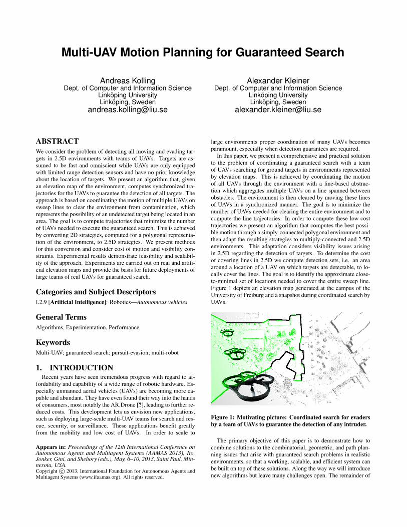
In this paper, we present a comprehensive and practical solutionto the problem of coordinating a guaranteed search with a teamof UAVs searching for ground targets in environments representedby elevation maps. This is achieved by coordinating the motionof all UAVs through the environment with a line-based abstrac-tion which aggregates multiple UAVs on a line spanned betweenobstacles. The environment is then cleared by moving these linesof UAVs in a synchronized manner. The goal is to minimize thenumber of UAVs needed for clearing the entire environment and tocompute the line trajectories. In order to compute these low costtrajectories we present an algorithm that computes the best possi-ble motion through a simply-connected polygonal environment andthen adapt the resulting strategies to multiply-connected and 2.5Denvironments. This adaptation considers visibility issues arisingin 2.5D regarding the detection of targets. To determine the costof covering lines in 2.5D we compute detection sets, i.e. an areaaround a location of a UAV on which targets are detectable, to lo-cally cover the lines. The goal is to identify the approximate close-to-minimal set of locations needed to cover the entire sweep line.Figure 1 depicts an elevation map generated at the campus of theUniversity of Freiburg and a snapshot during coordinated search byUAVs.
Figure 1: Motivating picture: Coordinated search for evadersby a team of UAVs to guarantee the detection of any intruder.
The primary objective of this paper is to demonstrate how tocombine solutions to the combinatorial, geometric, and path plan-ning issues that arise with guaranteed search problems in realisticenvironments, so that a working, scalable, and efficient system canbe built on top of these solutions. Along the way we will introducenew algorithms but leave many challenges open. The remainder of
this paper is organized as follows. In Section 2 related work is dis-cussed. Section 3 introduces the guaranteed search problem. Thefirst part of our approach, concerned with a simplified 2D variant,is described in Section 4. In Section 5 issues arising with complex2.5D environments are addressed. In Section 6 results from exper-iments on a variety of maps are presented and we finally concludewith Section 7.
2. RELATED WORKGuaranteed search, pursuit-evasion and other search problems
are at the cross-section between robotics, graph theory, computa-tional geometry and probability theory. Consequently, a wide rangeof models with different assumptions regarding environments, sen-sors, motion of robots or motion of targets exist and each contri-bution usually emphasizes a particular aspect of the problem fromtheoretical to practical. We shall briefly review a few of the mostclosely related works. An overview of guaranteed search and pursuit-evasion from a robotics perspective is given in the survey [?]. Asurvey, in form of an annotated bibliography, from the a graph the-ory perspective can be found in [?].
Real robotic systems for large scale guaranteed search with mul-tiple searchers are still rare and we are not aware of such systemswith UAVs and 2.5D or 3D environments. Combining solutionsto problems arising when using real robots with the more abstractcombinatorial and geometric methods has proven to be a consid-erable challenge. Smaller systems have been demonstrated suchas in [?]. The largest demonstration to date, with eight searchersin a 2.5D outdoor environment was presented in [?], although thesearchers were humans equipped with iPads and not actual robots.The work in [?] combined solutions to graph-theoretic pursuit-evasion problems [?] with a sampling-based analysis of the geom-etry and visibility of the 2.5D environment. In addition, to executethe search faster a time optimization was considered. In contrastto our work, [?] employed a graph-based approach and consideredstatic guarding locations while we consider a line-based approachwith moving lines and trajectories. Most contributions emphasizeoptimizing the number of searchers. A notable exception is [?]which deals with the computational complexity of optimizing thetime to execute search strategies on graphs. Yet, much further workin this domain remains to be done.
Another issue that did not receive much attention is that of graphswith cycles. Trees are fairly well understood for many of the pursuit-evasion problems [?, ?, ?] and in some case can be solved optimallyin polynomial time. Consequently, practical robotic applicationthat deal with complex environments with cycles turn to heuris-tics that convert graphs to trees and assume that additional searchercan be used to emulate this conversion in real environments. Suchapproaches have been used in [?, ?, ?] amongst others. In our workwe will also follow this approach.
Problems involving 2.5D and 3D environments, in conjunctionwith UAVs are also becoming more popular. In [?] and [?] UAVswere considered search with a single searcher and for tracking.For our purposes the closest related work in 2.5D is [?]. ThereinKleiner et al. consider the efficient computation of so called detec-tion sets that determine on which locations a UAV can see targetsin a 3D environment represented by a 2.5D elevation map.
Other related works deal with moving boundaries and lines ofrobots, usually ground robots, for example the coordination of se-curity sweeps for which market-based methods have been used[?] in 2D environments. Another 2D approach, from a control-theoretic perspective, is presented in [?]. Therein Durham et al.presented a distributed algorithm guaranteeing complete coverageof the frontier between cleared and contaminated areas during ex-
pansion [?]. Their algorithm can be applied to multiply-connectedplanar environments which may be non-polygonal, but no mini-mization of the number of robots is provided. Another approach us-ing sweep lines for clearing an environments by coordinating lineson a Voronoi diagram has been presented by Kolling et al. [?]. TheVoronoi Diagram of the environment induces a surveillance graphfor which the weights, i.e. costs in terms of UAVs, of vertices aregiven by the distances to the three closest and equidistant obstacles.Lines then either wait on a Voronoi edge or move towards a newobstacle that is associated to a Voronoi vertex. This approach wasshown in [?] to result in suboptimal coordination of lines for someproblem instances, which motivated our generalized approach pre-sented here. In contrast to [?] we consider more possibilities for theexpansion of the lines and provide a more flexible data structure forthe analysis of the environment leading to an improved algorithm.In addition we consider the adaptation of line-based strategies to2.5D environments with complex visibility constraints.
Another closely related paper by Efrat et al. [?] considers anapproach where multiple robots, each with an unlimited range sen-sor, are arranged in a single movable polygonal chain operating ina simply connected environment. Their algorithm for computingmotion strategies runs in O(n3), an improved version of the algo-rithms runs in O(n logn) time [?]. Our work in contrast considersUAVs with a limited sensing range, e.g. a downward facing cam-era, and multiple simultaneous lines in the environment. We furtherallow the number of lines to vary as the search mission unfolds.
3. PROBLEM DESCRIPTIONIn this section we describe our search problem in more detail. We
make similar assumptions as most pursuit-evasion problems withregard to target characteristics, namely a worst-case mobile targetthat can move with unbounded speed, is omniscient, and optimallyevasive. For robotic applications these assumptions have the ad-vantage that one can search for targets with unknown propertiesand still retain a guarantee of detection. From a theoretical per-spective we get the advantage that we can represent the possibilityof a target being present at a location with the concept of contam-ination. This then turns the detection of all worst-case targets intothe problem of removing all contamination and interesting formalquestions with regard to re-contamination can be addressed [?].
Our assumptions about the environments and searchers differfrom much of the prior work, with the exception of [?] from whichwe adapted our models. We assume a 2.5D environment E rep-resented by an elevation map h : H → R+. The domain H iscontinuous and H ⊂ R2 which, for all practical purposes, we willapproximate with a 2D grid map that contains in each discrete gridcell the corresponding height value. Let us write E ⊂ H and as-sume E is connected and every point in E is reachable by targetsfrom any other point in E . Targets are required to move on contin-uous paths in E , albeit as noted above with unbounded speed. Wedefine a path to be a continuous function π : [0, 1] → E . Hence,targets can be thought of as moving on the ground level of the el-evation map. The searchers are UAVs flying at a specified heighthr above the ground. The sensor model is a limited range disc of agiven sensing radius, representing a downward facing camera. LetR = {R1, R2, . . . , Rn} represent the n UAVs in E . Every Ri isdescribed by a path πi : [0, 1] → H , i.e. locations πi(t) ∈ H attime t, and an associated height hr above h(πi(t))
1.For every UAV Ri let D(πi(t)) ⊂ E be its sensor footprint, i.e.
the set of locations in E on which the UAV can detect targets. Ingeneral, D(πi(t)) depends on the sensor model, height of the UAV
1We assume all UAVs fly at the same height above the ground.
hr relative to h(πi(t)) and height of targets ht. In this paper weconsider a limited range, three-dimensional, and omni-directionalsensor with a sensing range of sr , the same model as described in[?]. A target at p′ ∈ H is hence detectable by a UAV Ri locatedat πi(t) at time t if at least one point on the line segment from{p′, h(p′)} to {p′, h(p′) + ht} embedded in R3 is visible from{pi, h(pi) +hr} at distance sr . Let D(t) :=
⋃i=1,...,nD(πi(t)))
be the joint sensor footprint of all UAVs at time t. We can nowdefine the concept of cleared and contaminated points in E .
DEFINITION 1 (CLEARED AND CONTAMINATED POINTS). Apoint x ∈ E is cleared at time t if x ∈ D(t). Furthermore, apoint x cleared at time t is also cleared at time t′ > t if @ a pathπ : [0, 1] → E from x to a contaminated point y ∈ E at any timet′′ ∈ [t, t′] that does not intersect D(t). If x is not clear it is calledcontaminated. At t = 0 all points in E \ (D(0)) are contaminated.
The problem now is to find the paths πi and the minimum num-ber of UAVs n, so that there exists for each UAV Ri a path πi :[0, 1] → E such that at t = 1 an initially contaminated environ-ment E is cleared. Since many of the pursuit-evasion problemsin simpler environments, such as graphs or even some variants ontrees, are already NP-hard we expect this problem to computation-ally difficult and are not going to be concerned with assessing itscomplexity. The remainder of the paper focuses on a multi-stepapproach to use simplified versions of the problem, address themseparately, and then successively combine them to finally lead topaths πi. These steps involve a coordination of motion on lines in2D, the generation of coverage location for lines in 2.5D, and thecomputation of trajectories from these locations.
4. 2D COORDINATIONTo tackle the problem of computing paths π1, . . . , πm that clear
all of E we first take a more abstract and simplified perspective in2D. Instead of individual UAVs we consider the joint sensor foot-prints of multiple UAVs and represent these with sweep lines thatmove through the environment. This representation of multipleUAVs as sweep lines enables us to coordinate their paths in or-der to minimize the number of UAVs needed for clearing the entireenvironment. For this, we assume that we are given a representa-tion of E in form of a simply-connected and simple polygon, P ={v1, . . . , vn}, with n vertices and edges, written ei = [vi, vi+1],i = 1, . . . , n. The edges ei of the polygon are then the obstaclesof the environment and we also interpret them, with slight abuse ofnotation, as straight line segments ei ⊂ R2. In Section 5 we dis-cuss how to deal with multiply-connected environments and how topolygonize the elevation map h introduced earlier. Throughout thissection the obstacle indices, i.e. the polygon edges, are assumed tobe circular, i.e. we identify i+ n with i.
The basic idea of coordinating the motion of UAVs on sweeplines is quite simple. A sweep line can be spanned between anytwo obstacles and it has an associated cost that represents the num-ber of UAVs needed to cover the area of the line with their sensors.The goal is to coordinate the motion of multiple such lines movingthrough the environment while minimizing the maximum cost thatoccurs at any point in time. The movement of these lines then clearsthe entire environment and every line separates the contaminatedfrom the cleared area. A more formal definition of the problem offinding a motion schedule for many sweep lines in a 2D environ-ment was formulated in [?] and we shall present a shortened andless formal introduction.
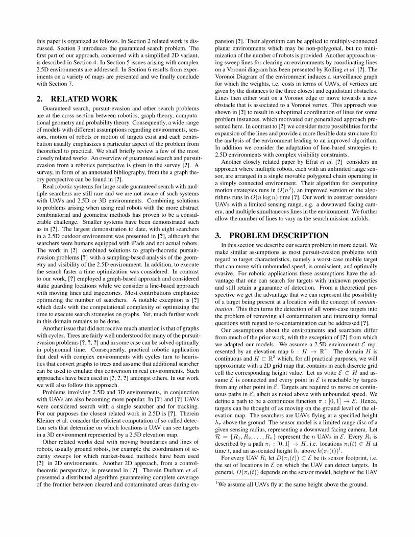
Initially, the interior of P is contaminated and one sweep linehas to start at some point on the obstacle boundary. Its initial mo-tion then clears the contamination in the area it sweeps over. This
is illustrated in Fig. 2. The role of these lines is either to continuesweeping the environment and expand the cleared area or to blockcontamination from entering the already cleared parts. Let C bethe cleared interior of P , then the intersection of the boundary ofC with interior of P has to have sweep lines on it that block con-tamination, i.e. δC ∩ interior(P ) is covered by lines with UAVson them. Otherwise C will get recontaminated. The problem is tofind lines and move them through the environment to clear it at thelowest cost in terms of UAVs without allowing the recontaminationof any point in C. For expanding the cleared area C and for block-
Figure 2: The beginning of a sweep through an environment us-ing lines. In a) the sweep starts with one line, extends by movingthe line through the interior and then splits into two lines, eachguarding two separate boundaries of the cleared area.
ing recontamination only sweep lines that are spanned between twoobstacles are useful. Note that we also consider sweep lines that arecomposed of multiple straight line segments. Let us write li,j fora sweep line between obstacles ei and ej . The cost of this sweepline is given by c(li,j) and represents the number of UAVs neededto cover the line. This cost function can defined appropriately for agiven environment or type of robot, but for our purpose we assumethat c(li,j) =
|li,j |2·sr , where sr is the sensor range of the UAVs and
|li,j | is the length of the line (Euclidean).Obviously, we need to find short lines in P between the obstacles
ei and ej . For this we assume that we have two basic functions.One that computes the shortest line between two edges ei, ej inP , called shortest(ei, ej), and one that computes the shortest linebetween a point p ∈ P and an edge ei in P , called shortest(ei, p).In a polygon, these shortest lines are simple to compute. We referthe reader to [?] Chapter 6.2.4 for details on planning shortest pathsbetween two points in polygons.
To keep track of C we call an edge ei of P cleared if C ∩ ei 6= ∅,i.e. if any point on ei is cleared. Now all cleared ei that havean adjacent obstacle that is still contaminated must have a sweepline starting on it to block contamination. Let ei and ej be twosegments which have a blocking sweep line between them and letlb(i, j) = shortest(ei, ej) denote the lowest cost line that blockscontamination.
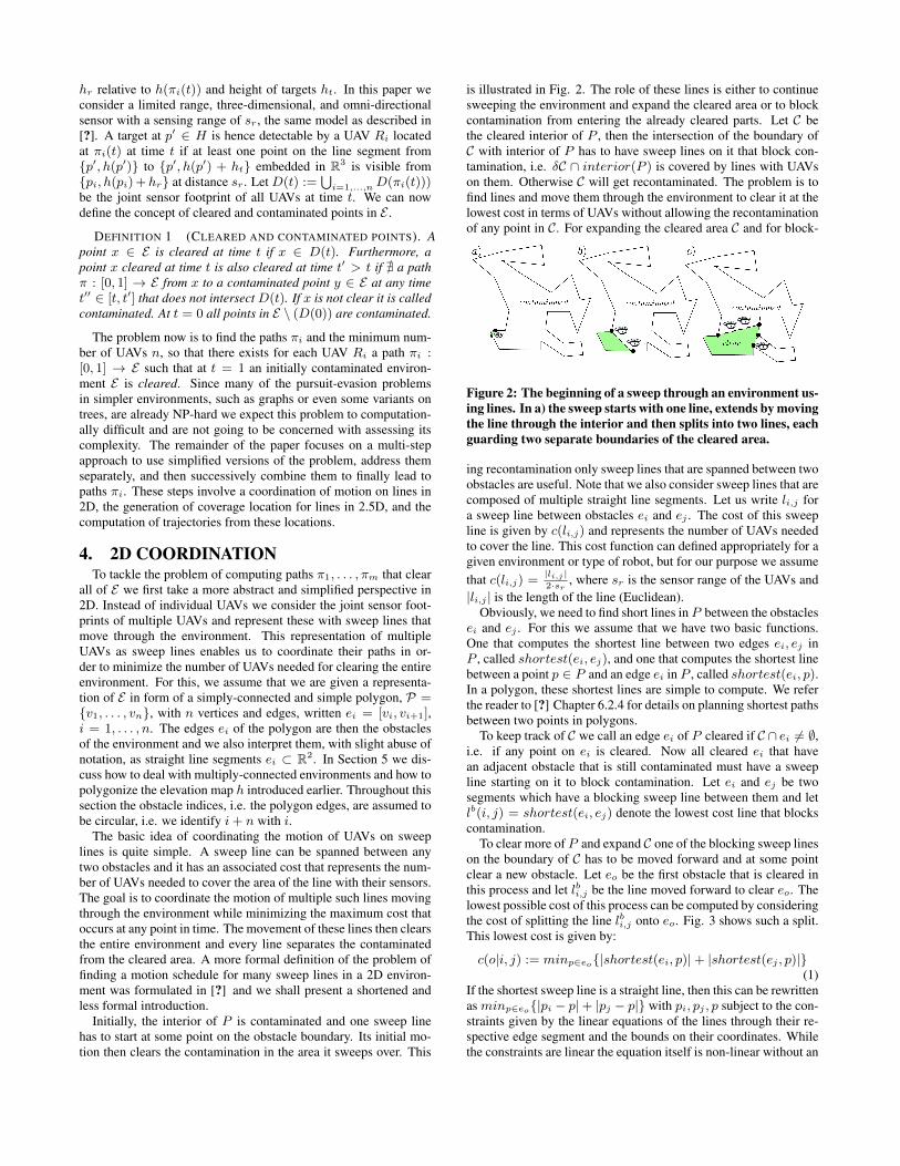
To clear more of P and expand C one of the blocking sweep lineson the boundary of C has to be moved forward and at some pointclear a new obstacle. Let eo be the first obstacle that is cleared inthis process and let lbi,j be the line moved forward to clear eo. Thelowest possible cost of this process can be computed by consideringthe cost of splitting the line lbi,j onto eo. Fig. 3 shows such a split.This lowest cost is given by:
c(o|i, j) := minp∈eo{|shortest(ei, p)|+ |shortest(ej , p)|}(1)
If the shortest sweep line is a straight line, then this can be rewrittenas minp∈eo{|pi − p|+ |pj − p|} with pi, pj , p subject to the con-straints given by the linear equations of the lines through their re-spective edge segment and the bounds on their coordinates. Whilethe constraints are linear the equation itself is non-linear without an
easy analytical solution. For our purposes we assume an oracle forEq. 1 that simply returns the point p. A sample implementation forsuch an oracle is given in a later section.
Once a line is split on a new obstacle, as illustrated in Fig. 3,we get blocking lines between eo and ei and eo and ej . The costto maintain these lines can be reduced by moving them to a lo-cally shorter line, namely lbi,o and lbj,o, as shown in Fig. 3. No-tice that if the index o is adjacent to either j, i, or both, then thelength of lbi,o, lbj,o, or both is zero. These local operations, to find
Figure 3: A line between ei and ej in a) splitting on eo in b) andmoving towards the blocking lines lb(i, k) and lb(j, k) in c).
a low cost blocking line or a low cost split, are relatively simple.The difficulty lies in coordinating many such operations in a largerenvironment and determining which line should split onto whichobstacles and in which sequence. Every choice of split furtherdetermines the possible choices and costs for future splits. A se-quence of all obstacle indices o1, . . . , on completely determineswhen and where to do a split. The first splits on o1 and o2 sim-ply set up the first line, possibly a zero length line if o1 and o2are adjacent. The s-th split, s > 2, is then given by os. The linethat is split on os is the blocking line between two indices fromo1, . . . , os−1. These indices are next smaller and next larger indexto os in o1, . . . , os−1, i.e. ol = argmaxo∈{o1,...,os−1}{o < os}and or = argmino∈{o1,...,os−1}{o > os}. So the line lb(ol, or)
is split on os while all other lines already present in P wait. Theoverall cost can be calculated by summing up all other blockinglines and the cost of the split onto os. A different obstacle se-quence o1, . . . , on will lead to a different sequence of splits, hencea different coordination of the motion of lines and potentially dif-ferent cost. In the next section we show how to compute obstaclesequence without having to consider all possible sequences. Thisleads to choices of the splits so that the overall cost is minimizedand based on this we can compute a low cost coordination of lines.
4.1 Choice SetsIn order to keep track of possible blocks and splits and their costs
we use the concept of a choice set, first introduced in [?]. Ev-ery choice set represents a consecutive set of indices that are stillcontaminated. These indices are the possible choices for splits ofthe blocking line that prevents the contamination of C. Now, sup-pose we have a contaminated area circumscribed by k consecutiveedges starting at edge ei, i.e. the sequence of edges with indices{i, i+ 1, . . . , i+ k − 1}. Write T i
k := {i, i+ 1, . . . , i+ k − 1},call T i
k a choice set, and let it represent the contaminated area cir-cumscribed by ei, . . . , ei+k−1. Write T i
0 = T0 = ∅ for all i. This
contaminated area is separated from the other parts of the environ-ment by a blocking line, written lb(T i
k) := lbi−1,i+k, going fromedge ei−1 to edge ei+k. As a shorthand write b(T i
k) := c(lb(T ik)),
the blocking cost for the contaminated T ik.
To continue clearing the area of T ik we can choose a split on
any index o ∈ T ik. Write c(o|T i
k) := c(o|i − 1, i + k) using Eq.1. Splitting on o will split the contaminated area for T i
k into twodisconnected contaminated areas. Each of these areas is again rep-resented by a choice set, namely T i
o−i to the left of o and T o+1i+k−o−1
to the right of o. For convenience we shall write T l = T io−i and
T r = T o+1i+k−o−1. Each of these in turn have their own blocking
lines and choices at a given cost. We can use the relationship ofT ik to T r and T l to construct the cost of obstacle sequences recur-
sively since T r, T l ⊂ T ik and their low cost obstacle sequences
are subsequences for low cost obstacles sequences of T ik. Using
this recursive construction we will take advantage of identifyingsubsequences that cannot possibly improve obstacles sequences inlarger choice sets. For this we will have to consider a fundamentalproblem for guaranteed search and pursuit-evasion. One of the keydifferences to other kinds of search problems is that once a certainsearch state, i.e. a cleared area, is reached there is a cost associ-ated with maintaining, i.e. blocking, it. For guaranteed search wehave to not only find lowest cost for extending the search state, butalso to keep track of the resulting maintenance costs. Hence, inour recursive construction of obstacle sequences we not only haveto consider sequences that have a low cost to clear a choice set, butalso those that have intermediate steps with a low blocking cost, butoverall higher clearing cost. The reason for this is that in combina-tion with other obstacle sequence during the recursive construction,not only the clearing cost, but the intermediate blocking cost maydetermine the overall cost of the combined sequence. This can bethe case if for T r we have high clearing costs and in T l we canreach a low blocking costs before clearing T r . This means we canchoose an obstacle sequence in T l with higher individual clearingcost, but lower intermediate blocking cost, in order to reduce thetotal cost for clearing the more expensive area for T r . In [?] a sim-ilar reasoning was used to develop the concept of full cut sequencesand compute optimal pursuit-evasion strategies on weighted trees.These full cut sequences are used to keep track of useful states andsequences in which intermediate costs for blocking are low andthat can be reached with a low clearing cost. In order to do this forobstacle sequences we first introduce their clearing and blockingcosts.
Let O = {o1, . . . , ok} be an obstacle sequence using all in-dices from T i
k, i.e. os ∈ T ik and os 6= os′ ⇐⇒ s 6= s′.
Write O for all such obstacle sequences. Computing the costs forthe resulting sweep lines of any O ∈ O is easily done by exe-cuting the splits in the given order and keeping track of the re-sulting costs for blocking all choice sets until they are all cleared.Let µs(O) be the cost of all sweep lines located in the area forT ki when splitting on os and let bs(O) be the cost of all sweep
lines after splitting on os, i.e. the blocking cost after step s. LetT isks
be the choice set so that os splits the line lis−1,is+ks ontoeos . Note that is = argmaxo∈{o1,...,os−1}{o < os} and ks =
argmino∈{o1,...,os−1}{o > os} − is − 1. Now, µs(O) and bs(O)are given by:
µs(O) = bs−1(O) + c(os|T isks
)− b(T isks
) (2)
bs(O) = bs−1(O)− b(T isks
) (3)
+b(T isos−is
) + b(T os+1is+ks−os−1) (4)
with b0(O) := c(li−1,i+k), i.e. the cost of the blocking line for
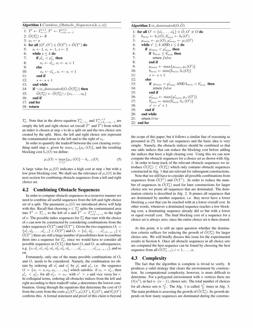
Algorithm 1 Combine_Obstacle_Sequences(k, i, o))
1: T l ← T i+1o−i , T r ← T o+1
i+k−o−1
2: O(T ik)← ∅
3: o1 ← o4: for all (Ol, Or) ∈ O(T l)× O(T r) do5: sl ← 1, sr ← 1, s← 26: while s ≤ k do7: if ρlsl < ρrsr then8: os ← olsl , sl ← sl + 19: else
10: os ← orsr , sr ← sr + 111: end if12: s← s+ 113: end while14: if ¬ is_dominated(O, O(T i
k)) then15: O(T i
k)← O(T ik) ∪ {o1, . . . , ok}
16: end if17: end for18: return
T ik. Note that in the above equation T is
os−isand T os+1
is+ks−os−1 aresimply the left and right choice set (recall T r and T l) from whichan index is chosen at step s to do a split on and the two choice setscreated by the split. Here, the left and right choice sets representthe contaminated areas to the left and to the right of os.
In order to quantify the tradeoff between the cost clearing every-thing until step s, given by maxs′≤s{µs′(O)}, and the resultingblocking cost bs(O) we define:
ρs(O) = maxs′≤s{µs′(O)} − bs−1(O). (5)
A large value for ρs(O) indicates a high cost at step s but with alow prior blocking cost. We shall see the relevance of ρs(O) in thenext section for combining obstacle sequences from a left and rightchoice set.
4.2 Combining Obstacle SequencesIn order to compute obstacle sequences in a recursive manner we
need to combine all useful sequences from the left and right choiceset of a split. The parameter ρs(O) we introduced above will helpwith this. Recall that choosing o ∈ T i
k splits the contaminated areainto T l = T i
o−i to the left of o and T r = T o+1i+k−o−1 to the right
of o. The possible index sequences for T ik that start with the choice
of o can now be constructed by considering combinations from theindex sequences O(T l) and O(T r). Given the two sequencesOl ={ol1, ol2, . . . , olo−i} ∈ O(T l) andOr = {or1, or2, . . . , ori+k−o−1} ∈O(T r) there are still a large number of possibilities how to combinethem into a sequence for T i
k, since we would have to consider allpossible sequences in O(T i
k) that haveOl andOr as subsequences,e.g. {o, ol1, or1, or2, or3, ol2, or4, or5, . . . , olo−i, . . . , o
ri+k−o−1}, and so
on.Fortunately, only one of the many possible combinations of Ol
and Or needs to be considered. Namely, the combination we ob-tain by ordering all ols and ors by ρls and ρrs, i.e. the sequenceO = {o1 = o, o2, o3, . . . , ok} which satisfies: if os = ols′ , thenρls′ < ρrs′′ for all ors′′ = os∗ with s∗ > s and vice versa for r.In colloquial terms, ordering all obstacles indices from the left andright according to their tradeoff value ρ determines the lowest com-bination. Going through the equations that determine the cost of Ofrom the costs from the costs µl
s(Ol), µls(Or), bls(Ol), and bls(Or)
confirms this. A formal statement and proof of this claim is beyond
Algorithm 2 is_dominated(O, O)
1: for all O′ = {o′1, . . . , o′k} ∈ O, O′ 6= O do2: bmin ← b1(O), b′min ← b1(O′)3: µmax ← µ1(O), µ′max ← µ1(O′)4: while s′ ≤ k AND s ≤ k do5: if µmax < µ′max then6: if bmin ≤ b′min then7: return false8: end if9: µmax ← max{µmax, µs(O′)}
10: bmin ← min{bmin, bs(O)}11: s← s+ 112: else13: if µmax = µ′max AND bmin < b′min then14: return false15: end if16: µ′max ← max{µ′max, µs′(O
′)}17: b′min ← min{b′min, bs′(O
′)}18: s′ ← s′ + 119: end if20: end while21: return true22: end for
the scope of this paper, but it follows a similar line of reasoning aspresented in [?] for full cut sequences and the basic idea is verysimple. Namely, the obstacle indices should be combined so thatone adds indices that can reduce the blocking cost before addingthe indices that have a high clearing cost. Using this we can nowcompute the obstacle sequences for a choice set as shown with Alg.1. In order to keep track of the relevant obstacle sequences we in-troduce O(T i
k) ⊂ O(T ik) which only contains obstacle sequences
constructed in Alg. 1 that are relevant for subsequent constructions.Note that we still have to consider all possible combinations from
sequences from O(T l) and O(T r). In order to reduce the num-ber of sequences in O(T i
k) used for later constructions for largerchoice sets we prune all sequences that are dominated. The dom-ination criteria is described in Alg. 2. It prunes all sequences thatare dominated by another sequence, i.e. they never have a lowerblocking µ cost that can be reached with at a lower overall cost. Inother words, whenever a dominated sequence reaches a low block-ing cost, a dominating sequence already did so but with a loweror equal overall cost. The final blocking cost of a sequence for achoice set is always zero, since the entire choice set is then cleared.
At this point, it is still an open question whether the domina-tion criteria suffices for reducing the growth of O(T i
k) for largerchoice sets. We will briefly discuss this issue for the experimentalresults in Section 6. Once all obstacle sequences in all choice setsare computed the best sequence can be found by choosing the bestsequence from all O(T i
n−1), i = 1, . . . , n.
4.3 ComplexityThe fact that the algorithm is complete is trivial to verify. It
produces a valid strategy that clears the environment by construc-tion. Its computational complexity, however, is more difficult todetermine. For a polygonal environment with n vertices there areO(n2), in fact n · (n−1), choice sets. The total number of choicesfor all choice sets is n3
2. The Alg. 1 is called n3
2times in Alg. 3.
The main problem is assessing the growth of O(T ik). Its growth de-
pends on how many sequences are dominated during the construc-
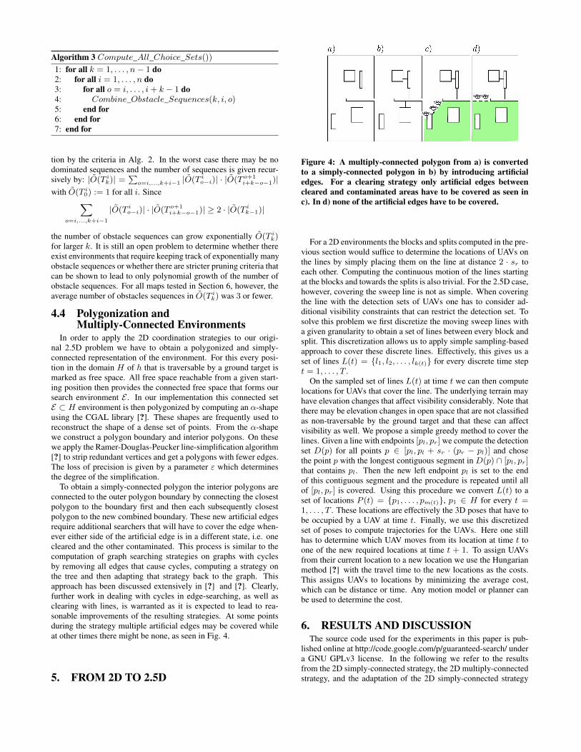
Algorithm 3 Compute_All_Choice_Sets())1: for all k = 1, . . . , n− 1 do2: for all i = 1, . . . , n do3: for all o = i, . . . , i+ k − 1 do4: Combine_Obstacle_Sequences(k, i, o)5: end for6: end for7: end for
tion by the criteria in Alg. 2. In the worst case there may be nodominated sequences and the number of sequences is given recur-sively by: |O(T i
k)| =∑
o=i,...,k+i−1 |O(T io−i)| · |O(T o+1
i+k−o−1)|with O(T i
0) := 1 for all i. Since∑o=i,...,k+i−1
|O(T io−i)| · |O(T o+1
i+k−o−1)| ≥ 2 · |O(T ik−1)|
the number of obstacle sequences can grow exponentially O(T ik)
for larger k. It is still an open problem to determine whether thereexist environments that require keeping track of exponentially manyobstacle sequences or whether there are stricter pruning criteria thatcan be shown to lead to only polynomial growth of the number ofobstacle sequences. For all maps tested in Section 6, however, theaverage number of obstacles sequences in O(T i
k) was 3 or fewer.
4.4 Polygonization andMultiply-Connected Environments
In order to apply the 2D coordination strategies to our origi-nal 2.5D problem we have to obtain a polygonized and simply-connected representation of the environment. For this every posi-tion in the domain H of h that is traversable by a ground target ismarked as free space. All free space reachable from a given start-ing position then provides the connected free space that forms oursearch environment E . In our implementation this connected setE ⊂ H environment is then polygonized by computing an α-shapeusing the CGAL library [?]. These shapes are frequently used toreconstruct the shape of a dense set of points. From the α-shapewe construct a polygon boundary and interior polygons. On thesewe apply the Ramer-Douglas-Peucker line-simplification algorithm[?] to strip redundant vertices and get a polygons with fewer edges.The loss of precision is given by a parameter ε which determinesthe degree of the simplification.
To obtain a simply-connected polygon the interior polygons areconnected to the outer polygon boundary by connecting the closestpolygon to the boundary first and then each subsequently closestpolygon to the new combined boundary. These new artificial edgesrequire additional searchers that will have to cover the edge when-ever either side of the artificial edge is in a different state, i.e. onecleared and the other contaminated. This process is similar to thecomputation of graph searching strategies on graphs with cyclesby removing all edges that cause cycles, computing a strategy onthe tree and then adapting that strategy back to the graph. Thisapproach has been discussed extensively in [?] and [?]. Clearly,further work in dealing with cycles in edge-searching, as well asclearing with lines, is warranted as it is expected to lead to rea-sonable improvements of the resulting strategies. At some pointsduring the strategy multiple artificial edges may be covered whileat other times there might be none, as seen in Fig. 4.
5. FROM 2D TO 2.5D
Figure 4: A multiply-connected polygon from a) is convertedto a simply-connected polygon in b) by introducing artificialedges. For a clearing strategy only artificial edges betweencleared and contaminated areas have to be covered as seen inc). In d) none of the artificial edges have to be covered.
For a 2D environments the blocks and splits computed in the pre-vious section would suffice to determine the locations of UAVs onthe lines by simply placing them on the line at distance 2 · sr toeach other. Computing the continuous motion of the lines startingat the blocks and towards the splits is also trivial. For the 2.5D case,however, covering the sweep line is not as simple. When coveringthe line with the detection sets of UAVs one has to consider ad-ditional visibility constraints that can restrict the detection set. Tosolve this problem we first discretize the moving sweep lines witha given granularity to obtain a set of lines between every block andsplit. This discretization allows us to apply simple sampling-basedapproach to cover these discrete lines. Effectively, this gives us aset of lines L(t) = {l1, l2, . . . , lk(t)} for every discrete time stept = 1, . . . , T .
On the sampled set of lines L(t) at time t we can then computelocations for UAVs that cover the line. The underlying terrain mayhave elevation changes that affect visibility considerably. Note thatthere may be elevation changes in open space that are not classifiedas non-traversable by the ground target and that these can affectvisibility as well. We propose a simple greedy method to cover thelines. Given a line with endpoints [pl, pr] we compute the detectionset D(p) for all points p ∈ [pl, pl + sr · (pr − pl)] and chosethe point p with the longest contiguous segment in D(p) ∩ [pl, pr]that contains pl. Then the new left endpoint pl is set to the endof this contiguous segment and the procedure is repeated until allof [pl, pr] is covered. Using this procedure we convert L(t) to aset of locations P (t) = {p1, . . . , pm(t)}, p1 ∈ H for every t =1, . . . , T . These locations are effectively the 3D poses that have tobe occupied by a UAV at time t. Finally, we use this discretizedset of poses to compute trajectories for the UAVs. Here one stillhas to determine which UAV moves from its location at time t toone of the new required locations at time t + 1. To assign UAVsfrom their current location to a new location we use the Hungarianmethod [?] with the travel time to the new locations as the costs.This assigns UAVs to locations by minimizing the average cost,which can be distance or time. Any motion model or planner canbe used to determine the cost.
6. RESULTS AND DISCUSSIONThe source code used for the experiments in this paper is pub-
lished online at http://code.google.com/p/guaranteed-search/ undera GNU GPLv3 license. In the following we refer to the resultsfrom the 2D simply-connected strategy, the 2D multiply-connectedstrategy, and the adaptation of the 2D simply-connected strategy
to 2.5D paths. More precisely, using the methods described in theabove sections, we carried out experiments relating to the followingquestions: 1) growth of O(T i
k); 2) feasibility and demonstration ina large real elevation map and the cost of adapting 2D strategiesto 2.5D; 3) cost of adapting strategies from simply-connected tomultiply-connected polygons; 4) scaling of the number of robotswith increasing environment size. To address these questions weused one realistic elevation map of the University of Freiburg seenin Fig. 5, and four mazes of different size seen in Fig. 6. Theresults are summarized in Table 1.
1) Growth of O(T ik): An investigation of the growth of O(T i
k)
showed that |O(T ik)| does not grow exponentially, but is constant
with an average around 3 for all the maps considered here. Thisshows that for the maps presented here most sequences are domi-nated by some few obstacle sequences with low clearing and block-ing costs. We conjecture that one can, in fact, show that the simply-connected 2D strategies are optimal and that the algorithm is poly-nomial. A proof of this conjecture is a promising direction for fur-ther work.
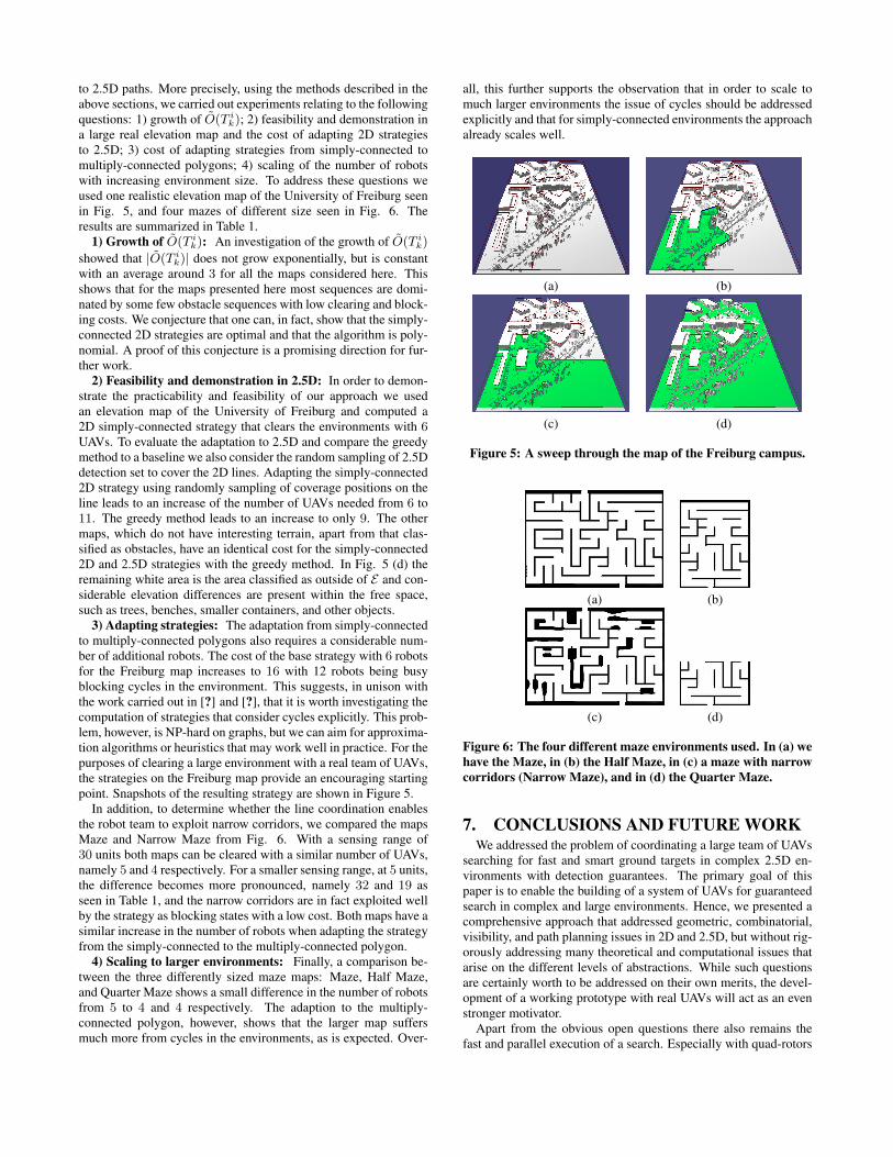
2) Feasibility and demonstration in 2.5D: In order to demon-strate the practicability and feasibility of our approach we usedan elevation map of the University of Freiburg and computed a2D simply-connected strategy that clears the environments with 6UAVs. To evaluate the adaptation to 2.5D and compare the greedymethod to a baseline we also consider the random sampling of 2.5Ddetection set to cover the 2D lines. Adapting the simply-connected2D strategy using randomly sampling of coverage positions on theline leads to an increase of the number of UAVs needed from 6 to11. The greedy method leads to an increase to only 9. The othermaps, which do not have interesting terrain, apart from that clas-sified as obstacles, have an identical cost for the simply-connected2D and 2.5D strategies with the greedy method. In Fig. 5 (d) theremaining white area is the area classified as outside of E and con-siderable elevation differences are present within the free space,such as trees, benches, smaller containers, and other objects.
3) Adapting strategies: The adaptation from simply-connectedto multiply-connected polygons also requires a considerable num-ber of additional robots. The cost of the base strategy with 6 robotsfor the Freiburg map increases to 16 with 12 robots being busyblocking cycles in the environment. This suggests, in unison withthe work carried out in [?] and [?], that it is worth investigating thecomputation of strategies that consider cycles explicitly. This prob-lem, however, is NP-hard on graphs, but we can aim for approxima-tion algorithms or heuristics that may work well in practice. For thepurposes of clearing a large environment with a real team of UAVs,the strategies on the Freiburg map provide an encouraging startingpoint. Snapshots of the resulting strategy are shown in Figure 5.
In addition, to determine whether the line coordination enablesthe robot team to exploit narrow corridors, we compared the mapsMaze and Narrow Maze from Fig. 6. With a sensing range of30 units both maps can be cleared with a similar number of UAVs,namely 5 and 4 respectively. For a smaller sensing range, at 5 units,the difference becomes more pronounced, namely 32 and 19 asseen in Table 1, and the narrow corridors are in fact exploited wellby the strategy as blocking states with a low cost. Both maps have asimilar increase in the number of robots when adapting the strategyfrom the simply-connected to the multiply-connected polygon.
4) Scaling to larger environments: Finally, a comparison be-tween the three differently sized maze maps: Maze, Half Maze,and Quarter Maze shows a small difference in the number of robotsfrom 5 to 4 and 4 respectively. The adaption to the multiply-connected polygon, however, shows that the larger map suffersmuch more from cycles in the environments, as is expected. Over-
all, this further supports the observation that in order to scale tomuch larger environments the issue of cycles should be addressedexplicitly and that for simply-connected environments the approachalready scales well.
(a) (b)
(c) (d)
Figure 5: A sweep through the map of the Freiburg campus.
(a) (b)
(c) (d)
Figure 6: The four different maze environments used. In (a) wehave the Maze, in (b) the Half Maze, in (c) a maze with narrowcorridors (Narrow Maze), and in (d) the Quarter Maze.
7. CONCLUSIONS AND FUTURE WORKWe addressed the problem of coordinating a large team of UAVs
searching for fast and smart ground targets in complex 2.5D en-vironments with detection guarantees. The primary goal of thispaper is to enable the building of a system of UAVs for guaranteedsearch in complex and large environments. Hence, we presented acomprehensive approach that addressed geometric, combinatorial,visibility, and path planning issues in 2D and 2.5D, but without rig-orously addressing many theoretical and computational issues thatarise on the different levels of abstractions. While such questionsare certainly worth to be addressed on their own merits, the devel-opment of a working prototype with real UAVs will act as an evenstronger motivator.
Apart from the obvious open questions there also remains thefast and parallel execution of a search. Especially with quad-rotors
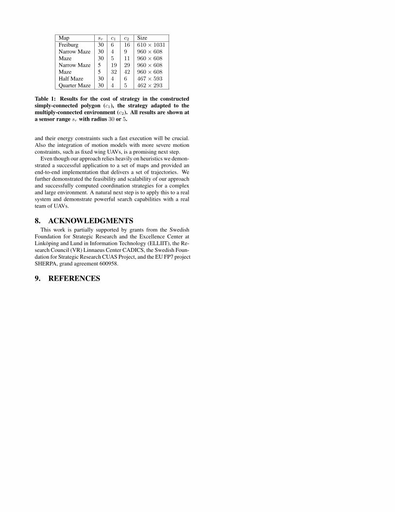
Map sr c1 c2 SizeFreiburg 30 6 16 610× 1031Narrow Maze 30 4 9 960× 608Maze 30 5 11 960× 608Narrow Maze 5 19 29 960× 608Maze 5 32 42 960× 608Half Maze 30 4 6 467× 593Quarter Maze 30 4 5 462× 293
Table 1: Results for the cost of strategy in the constructedsimply-connected polygon (c1), the strategy adapted to themultiply-connected environment (c2). All results are shown ata sensor range sr with radius 30 or 5.
and their energy constraints such a fast execution will be crucial.Also the integration of motion models with more severe motionconstraints, such as fixed wing UAVs, is a promising next step.
Even though our approach relies heavily on heuristics we demon-strated a successful application to a set of maps and provided anend-to-end implementation that delivers a set of trajectories. Wefurther demonstrated the feasibility and scalability of our approachand successfully computed coordination strategies for a complexand large environment. A natural next step is to apply this to a realsystem and demonstrate powerful search capabilities with a realteam of UAVs.
8. ACKNOWLEDGMENTSThis work is partially supported by grants from the Swedish
Foundation for Strategic Research and the Excellence Center atLinköping and Lund in Information Technology (ELLIIT), the Re-search Council (VR) Linnaeus Center CADICS, the Swedish Foun-dation for Strategic Research CUAS Project, and the EU FP7 projectSHERPA, grand agreement 600958.
9. REFERENCES