Multi-Variable Branching:

A Case Study with 0-1 Knapsack Problems

Yu Yang Natashia Boland Martin SavelsberghH. Milton Stewart School of Industrial and Systems Engineering

Georgia Institute of Technology

Atlanta, Georgia 30332

Abstract

We explore the benefits of multi-variable branching strategies for linear programming basedbranch and bound algorithms for the 0-1 knapsack problem, i.e., of branching on sets of vari-ables rather than on a single variable (the current default in integer programming solvers). Wepresent examples where multi-variable branching shows advantage over single-variable branch-ing, and partially characterize situations in which this happens. We show that for the class of0-1 knapsack instances introduced by Chvatal (1980) to demonstrate that linear programmingbranch and bound algorithms (employing a single-variable branching scheme) must exploreexponentially many nodes, a linear programming branch and bound algorithm employing amulti-variable branching scheme can solve any instance in either three or seven nodes. Finally,we investigate the performance of various multi-variable branching strategies computationally,and demonstrate their potential.

1 Introduction

Branch and bound, first proposed by Land and Doig (1960), has grown into a standard frameworkfor solving discrete optimization problems. Using bounds on the optimal solution value to avoidsearching parts of the solution space that cannot contain an optimal solution, branch and boundcan be far more effective than exhaustive search. We focus on linear programming based branchand bound for solving integer programs, which is the algorithmic framework at the heart of allcommercial, and most open source, software for solving integer programs. As dual bounds at thenodes in the search tree are obtained by solving the linear programming relaxation of the integerprogram at the nodes, the branching scheme employed has a significant impact on the effectivenessof the algorithm. The typical branching scheme identifies a variable xi with fractional value f inthe solution to the linear programming relaxation and creates two branches (i.e., two new nodes inthe search tree) one in which the constraint xi ≥ dfe is imposed and one in which the constraintxi ≤ bfc is imposed, i.e., branching is based on a single-variable dichotomy. As a result, mostresearch on branching schemes (in the context of linear programming based branch and bound) hasfocused on the identification of the variable to branch on, e.g., pseudo-cost branching (Benichouet al. 1971), strong branching (Applegate et al. 1995), and reliability branching (Achterberg et al.2005). Branching based on sets of variables, the focus of our research, has only been consideredin very special cases, e.g., special ordered set branching (see Beale and Tomlin (1970) and Beale

1

(1979)). We note that in their recent survey, Morrison et al. (2016) list multi-variable branchingschemes as one of the under-explored areas of research that deserves further investigation.

A multi-variable branching scheme is a natural generalization of a single-variable branchingscheme. Rather than branching on a single variable with a fractional value in the solution to thelinear programming relaxation, branching is performed on a set of variables such that the sum oftheir values in the solution to the linear programming relaxation is fractional. More specifically, aset S of variables with

∑i∈S xi = f with f fractional is identified and two branches are created, one

in which the constraint∑

i∈S xi ≥ dfe is imposed and one in which the constraint∑

i∈S xi ≤ bfcis imposed. In this case, of course, the question becomes how to choose the set S.

The “desirability” of branching on a particular variable in a single-variable branching schemeis commonly defined by the value max{z−, z+}, in case of a maximization problem, where z−

and z+ represent the optimal value of the linear programming relaxation on the “down” branchand the “up” branch, respectively, and where a smaller value of max{z−, z+} is more desirable.The same definition can be used to define the desirability of branching on a particular set ofvariables in a multi-variable branching scheme. We note that evaluating the desirability of everyfractional variable, in the context of a single-variable branching scheme, has been shown to leadto small search trees, but not necessarily to shorter solution time, as the evaluation of desirabilityis expensive (it involves solving two linear programs for each evaluation). This highlights one ofthe major challenges for the use of multi-variable branching schemes: evaluating the desirabilityof every possible set of variables such that the sum of their values in the solution to the linearprogramming relaxation is fractional will be computationally prohibitive.

To explore the benefit of multi-variable branching schemes, we focus on the 0-1 knapsack prob-lem, i.e., on the integer program of the following form:

maxn∑

i=1

pixi

subject ton∑

i=1

wixi ≤ b,

xi ∈ {0, 1}, ∀ i ∈ [n].

where [n] = {1, . . . , n} and b ∈ Z>0, pi, wi ∈ Z>0 and wi ≤ b for all i ∈ [n].Chvatal (1980) introduced a class of 0-1 knapsack instances to demonstrate that linear program-

ming branch and bound algorithms employing a single-variable branching scheme have to exploreexponentially many nodes. One of our contributions is to show that there is a linear program-ming branch and bound algorithm employing a multi-variable branching scheme that can solveany instance in this class by exploring either three or seven nodes. Another contribution is thatwe present and partially characterize situations in which multi-variable branching schemes lead tobetter dual bounds, i.e., smaller values of max{z−, z+}, which should lead to smaller search trees.Finally, we demonstrate the potential benefits of multi-variable branching scheme in an extensivecomputational study in which we assess the performance of various branching schemes, where ourprimary measure for the quality of a branching scheme is the number of nodes explored in thesearch tree, but, at the same time, we seek branching schemes that are computationally efficient.

For completeness and to establish notation, we include a high-level description of the LP-basedbranching and bound algorithm for maximizing a 0-1 integer program used in our research inAlgorithm 1, where L denotes the list of active 0-1 integer programs, xbest denotes the incumbent

2

with objective value zbest, and zUPi an upper bound on the value of the 0-1 integer program Pi at

node i.

Algorithm 1: LP-based branch and bound algorithm.

Initialization: L = {original 0-1 integer program} and zbest = −∞.while L 6= ∅ do

Select and remove a 0-1 integer program Pi from L.Solve the LP relaxation of Pi.if the LP relaxation is feasible then

Retrieve the LP solution xLPi and its objective value zLPi .if zLPi > zbest then

if xLPi is integer feasible thenxbest ← xLPi and zbest ← zLPi

Remove 0-1 integer programs Pj from L with zUBj ≤ zbest.

elseApply a branching strategy to create two new 0-1 integer programs Pi,1 andPi,2, set zUP

i,1 = zUPi,2 = zLPi , and add Pi,1 and Pi,2 to L.

The remainder of the paper is organized as follows. In Section 2, we review relevant literatureon branching paradigms. In Section 3, we consider a class of difficult 0-1 knapsack problemsintroduced by Chvatal. In Section 4, we give examples showing that branching on sets of variablescan be better than branching on a single variable, and derive conditions for branching on sets oftwo variables to be better than branching on a single variable. In Section 5, we report the resultsof a number of numerical experiments which further reinforce that branching on sets of variablesholds promise. Finally, in Section 6, we provide some concluding remarks.

2 Relevant Literature

2.1 Single variable selection

Over the years, much effort has been devoted to finding schemes for selecting a (single) variable tobranch on that result in small search trees. The simplest scheme is to select the variable xi withfractional part f − bfc closest to 0.5. Let z be the value of the linear programming solution. Theintuition (or hope) is that enforcing xi ≤ bfc and enforcing xi ≥ dfe result in noticeable changesto the value of the linear program, and, therefore, we will have max{z−, z+} noticeably less thanz, which improves the dual bound. The computational requirements of this naive method areminimal, but, unfortunately, studies have shown that it is not much better than randomly selectinga variable (Achterberg 2007).

Rather than hoping that max{z−, z+} is noticeably less than z, pseudo-cost branching (PB)(Benichou et al. 1971) observes and records actual changes to the values of the linear programmingrelaxations and maintains for each variable xi an average change and uses these values to choosea variable to branch on. The major weakness of PB is that initially little or no information isavailable and initial branching decision, at the top of the search, are critically important. However,the computational requirements of PB are minimal, and computational studies have shown that itperforms reasonably well.

3

Rather than hoping or observing and recording, strong branching (SB) (Applegate et al. 1995)goes ahead and computes the change in dual bound for each variable xi with a fractional value,i.e., it computes the value z−i at the “down” child where xi ≤ bfic is imposed and the value z+i atthe “up” child where xi ≥ dfie is imposed. SB then chooses the variable xi for which max{z−i , z

+i }

is the smallest. SB results in small search trees, but, unfortunately, is computational intensive andthe benefits of smaller search trees are often undone by the effort required to select the variable tobranch on.

Hybrid strong / pseudo-cost branching tries to overcome the weaknesses of the two methods byapplying SB to nodes high in the search tree (i.e., depth up to d) and switching to PB for nodeslow in the search tree (i.e., depth more than d). Since d is typically chosen to be relatively small,fractional variables without a pseudo-cost may still be encountered at depth more than d, in whichcase SB is used to initialize the pseudo-cost (Gauthier and Ribiere 1977, Linderoth and Savelsbergh1999). These idea have been taken one step further in reliability branching (RB) (Achterberg et al.2005) which uses SB to initialize variables without a pseudo-cost or to re-initialize variables withan unreliable pseudo-cost. Extensive computational experiments have shown that RB performs thebest among all aforementioned methods in terms of solution time.

The recent success of machine learning has inspired new ways to guide the selection of thebranching variable. Di Liberto et al. (2016) introduce DASH (Dynamic Approach for SwitchingHeuristics) which chooses a branching scheme from a collection of branching schemes to be appliedat a node in the search tree based on the features of the integer program at that node. Thelearning is offline, i.e., it is based on the performance of the branching schemes on a set of traininginstances. Marcos Alvarez et al. (2017) seek to use machine learning to derive a branching schemethat mimics strong branching in the hopes of achieving small search trees without the need tospend huge amounts of computing to select a variable to branch on. Again, the learning is offline.An online learning variant enhanced by a reliability mechanism is proposed in Marcos Alvarezet al. (2016). Khalil et al. (2016) also employ online learning to mimic SB. The novelty of theirapproach lies in that the learning involves solving a ranking problem rather than using regressionor classification. The learning based branching methods do not yet outperform state-of-the-artimplementations of RB, but are able to achieve better results than PB or hybrid SB / PB. For arecent survey and more in-depth discussion of learning and branching for integer programming, seeLodi and Zarpellon (2017).

2.2 Multi-variable branching

Two types of special ordered sets (SOS) were introduced in Beale and Tomlin (1970) for modelingnonconvex problems. Special order sets of type 1 (SOS1), in which at most one element from anordered set can have a non-zero value, can be used to model multiple choice problems, while specialordered sets of type 2 (SOS2), in which up to two consecutive elements from an order set canhave non-zero values, can be used when a nonlinear function is approximated by a piecewise linearfunction. Multi-variable branching can be readily applied to variables appearing in special orderedsets. For example, let xi for i ∈ {1, . . . , n} be the variables in a special ordered set of type 1, and letx0 = x1 = . . . xk−1 = 0, xk = xk+1 = 0.5, and xk+2 = . . . , xn = 0, then we can branch by imposingxi = 0 for i = 1, . . . , k on one branch and imposing xi = 0 for i = k+ 1, . . . , n on the other branch.Similar branching ideas can be developed for special ordered sets of type 2. Beyond the well-knownSOS1 and SOS2, Beale (1979) also introduced Linked Ordered Sets (LOS). We note that thesemulti-variable branching rules target special structures occurring in certain types of optimization

4

problems.Basis reduction methods, following the groundbreaking work of Lenstra, Jr. (1983), also give

rise to multi-variable branching, often referred to as hyperplane branching in that context. (For anintroduction to basis reduction methods, see Pataki and Tural (2011), and for an overview of “non-standard” methods for integer programming, see Aardal et al. (2002).) Krishnamoorthy and Pataki(2009) demonstrate the potential of hyperplane branching for decomposable knapsack problems(DKPs). They demonstrate how to generate a feasibility version of 0-1 knapsack instances andshow how infeasibility can be proven by branching on hyperplanes (they also consider the Chvatalinstances we consider in Section 3). However, computing the desired hyperplanes involves basisreduction computations which are time-consuming in spite of their polynomial complexity for fixeddimension.

3 Chvatal Instances and Multi-Variable Branching

First, we demonstrate the potential of multi-variable branching on a class of 0-1 knapsack probleminstances introduced by Chvatal (1980). The class of instances is characterized by the followingformulation:

max

n∑i=1

aixi

subject to

n∑i=1

aixi ≤

⌊n∑

i=1

ai/2

⌋,

xi ∈ {0, 1}, i ∈ {1, . . . , n},

where

•∑

i∈I ai ≤∑n

i=1 ai/2 for all sets I ⊆ {1, . . . , n} with |I| ≤ n/10,

• every integer greater than one divides fewer than 9n/10 of the integers ai,

•∑

i∈I ai 6=∑

j∈J aj , when I 6= J , and

• there is no set I such that∑

i∈I ai = b∑n

i=1 ai/2c.

Chvatal (1980) shows that for this class of 0-1 knapsack instances, a linear programming basedbranch and bound algorithm employing a singe-variable branching scheme must explore at least2n/10 nodes.

Chvatal (1980) also considers a “specific example” with aj = 2k+n+1 + 2k+j + 1 for j = 1, . . . , nand with k = blog(2n)c. For this class of 0-1 knapsack instances, it can be shown that a linearprogramming based branch and bound algorithm employing a singe-variable branching scheme mustexplore at least 2(n−1)/2 nodes. We will show, for this class of instances, that a linear programmingbased branch and bound algorithm employing an appropriately chosen multi-variable branchingscheme solves instances by evaluating at most 7 nodes. We start by observing some properties ofthe instance data and showing that each instance has a unique optimal solution.

5

Lemma 1. When n is odd, the sum of the largest n−12 coefficients in the “specific example” is less

than b, while the sum of the smallest n+12 coefficients exceeds b:

n∑j=n+1

2+1

aj < b and

n+12∑

j=1

aj > b. (3.1)

Proof. For n odd,

b :=

⌊n∑

i=1

ai/2

⌋=

n∑j=1

(2k+n + 2k+j−1 + 1/2

) = (n+ 1)2k+n − 2k +n− 1

2.

Summing the largest n−12 elements, we have

n∑j=n+1

2+1

aj =n∑

j=n+12

+1

(2k+n+1 + 2k+j + 1

)= (n+ 1)2k+n − 2k+

n+12

+1 +n− 1

2< b. (3.2)

Summing the smallest n+12 elements, we have

n+12∑

j=1

aj =

n+12∑

j=1

(2k+n+1 + 2k+j + 1

)= (n+ 1)2k+n + 2k+

n+12

+1 − 2k+1 +n+ 1

2> b. (3.3)

�

Corollary 1. When n is odd, the inequality

n∑j=1

xj <n+ 1

2

is valid for the LP relaxation of the “specific example”.

Proof. This is obvious from the second part of Lemma 1. �

Corollary 2. When n is odd, the optimal solution to an instance in the “specific example” classis:

x∗ = (

n+12︷ ︸︸ ︷

0, . . . , 0,

n−12︷ ︸︸ ︷

1, . . . , 1).

Proof. By Corollary 1 and integrality, an optimal solution can have at most n+12 −1 = n−1

2 non-zerovariables. By Lemma 1, packing the last n−1

2 items into the knapsack is feasible, and since thesehave the largest coefficients, will give the best possible value. �

Proposition 1. If n is even, the optimal solution to an instance in the “specific example” class is:

x∗ = (0, . . . , 0︸ ︷︷ ︸n2−1

, 1, . . . , 1︸ ︷︷ ︸n2

, 0).

6

Proof. When n is even,

b =

⌊n∑

i=1

ai/2

⌋=

n∑j=1

(2k+n + 2k+j−1 + 1/2

) = (n+ 1)2k+n − 2k +n

2.

Summing the smallest n2 elements, we have

n2∑

j=1

aj =

n2∑

j=1

(2k+n+1 + 2k+j + 1

)= n2k+n + 2k+

n2+1 − 2k+1 +

n

2< b. (3.4)

Summing the first n2 + 1 elements, we have

n2+1∑

j=1

aj =

n2+1∑

j=1

(2k+n+1 + 2k+j + 1

)= (n+ 2)2k+n + 2k+

n2+2 − 2k+1 +

n

2+ 1 > b. (3.5)

Thus, we can pack at most n2 items. The most valuable n

2 items have total weight

n∑j=n

2+1

aj =

n∑j=n

2+1

(2k+n+1 + 2k+j + 1

)= (n+ 1)2k+n + 2k+n − 2k+

n2+1 +

n

2> b,

and, thus, we cannot simply pack the last n2 items. However, note thatn

2−1∑

j=1

aj

+an =

n2−1∑

j=1

(2k+n+1 + 2k+j + 1

)+2k+n+1+2k+n+1 = (n+2)2k+n+2k+n2−2k+1+

n

2> b.

(3.6)This shows that if the n-th item is included, we can pack at most n

2 − 1 items with total value nomore than

α :=

n∑j=n

2+2

aj =

n∑j=n

2+2

(2k+n+1 + 2k+j + 1

)= n2k+n − 2k+

n2+1 +

n

2− 1. (3.7)

Excluding the n-th item and packing the most valuable n2 items among the remaining n− 1 items

has value

α <

n−1∑j=n

2

aj =

n−1∑j=n

2

(2k+n+1 + 2k+j + 1

)= (n+ 1)2k+n − 2k+

n2 +

n

2< b. (3.8)

Thus, we obtain that the optimal solution is x∗ = (0, . . . , 0︸ ︷︷ ︸n2−1

, 1, . . . , 1︸ ︷︷ ︸n2

, 0). �

Next, we define the multi-variable branching scheme to be used for this class of instances. Let xbe the solution to the LP relaxation at a node, let X1 = {i : xi = 1, i ∈ [n]} be the set of variableswith value 1 in that solution, X0 = {i : xi = 0, i ∈ [n]} be the set of variables with value 0 inthat solution, Xf = {i : 0 < xi < 1, i ∈ [n]} be the set of variables with a fractional value in thatsolution, and j = min{i : i ∈ Xf} be the index of the first variable with a fractional value. Thenwe branch on the set S = X1 ∪X0 ∪ {j}.

7

Theorem 1. An LP-based branch and bound algorithm employing a multi-variable branching basedon the set S as defined above solves an instance in at most 7 nodes when n is even and at most 3nodes when n is odd.

Proof. We introduce the following notation. The root node of the search tree is identified by (0, ·)and other nodes are identified either by a pair (k,+) or by a pair (k,−) where k represents thedepth of the node, − indicates the node was reached from its parent by branching down, and +indicates the node was reached from its parent by branching up. In general, this does not uniquelyidentify a node in the search tree, but, as we will see shortly, in this case it does. The solution x(0,·)

at the root node has at most one fractional variable, which implies that S = [n].

When n is odd, by Lemma 1, we have n−12 <

∑ni=1 x

(0,·)i < n+1

2 . Branching on S = [n] generates

two branches defined by∑n

i=1 xi ≤n−12 and

∑ni=1 xi ≥

n+12 . By Lemma 1, LP(1,+) is infeasible,

while LP(1,−) has solution x(1,−) = (0, . . . , 0︸ ︷︷ ︸n+12

, 1, . . . , 1︸ ︷︷ ︸n−12

), which is the optimal solution to the instance.

Thus, in this case, at most 3 nodes are evaluated.

When n is even, by (3.5),∑n

i=1 x(0,·)i < n

2 + 1. By reasoning in the proof of Proposition 1,n2 − 1 <

∑ni=1 x

(0,·)i . To see this, suppose otherwise, i.e., suppose n

2 − 1 ≥∑n

i=1 x(0,·)i . In this case,

the objective value of x(0,·) cannot be better than that obtained by packing the n2 −1 most valuable

items, given by α in (3.7). But α < z∗, the value of the integer program, which cannot exceed thevalue of the LP relaxation (which must be b).

We consider several cases for∑n

i=1 x(0,·)i in the open interval (n2 − 1, n2 + 1).

Case 1: n2 − 1 <

∑ni=1 x

(0,·)i < n

2 . Branching on S = [n] generates two branches defined by∑ni=1 xi ≤

n2 − 1 and

∑ni=1 xi ≥

n2 . For LP(1,−), it is easy to see that the solution is x(1,−) =

(0, . . . , 0︸ ︷︷ ︸n2+1

, 1, . . . , 1︸ ︷︷ ︸n2−1

), which is integer but not optimal. Next, we analyze two subcases for LP(1,+).

(The search trees are shown in Figure 1.)

Case 1(a): If solution x(1,+) has exactly one fractional component, then S = [n] and n2 <∑n

i=1 x(1,+)i < n

2 + 1. Branching on S = [n] generates two branches defined by∑n

i=1 xi ≤n2 and∑n

i=1 xi ≥n2 + 1. Clearly, LP(2,+) is infeasible. Observe that LP(2,−) has both

∑ni=1 xi ≤

n2 and∑n

i=1 xi ≥n2 , which implies that

∑ni=1 xi = n

2 , which forces x(2,−) to have exactly two fractional

variables. One of them has to be xn, because if x(2,−)n = 0, it will not give the largest possible value

by (3.7) and (3.8). If x(2,−)n = 1, even if all n

2 − 1 items with smallest weight are included, i.e.,a1 through an

2−1, the weight constraint is still violated in view of (3.6). Therefore, at this node,

S = [n− 1], which generates two branches defined by∑n−1

i=1 xi ≤n2 − 1 and

∑n−1i=1 xi ≥

n2 . LP(3,−)

has both∑n

i=1 xi = n2 and

∑n−1i=1 xi ≤

n2 − 1, which implies xn = 1 and

∑n−1i=1 xi = n

2 − 1, which

is infeasible. LP(3,+) has solution x(3,+) = (0, . . . , 0︸ ︷︷ ︸n2−1

, 1, . . . , 1︸ ︷︷ ︸n2

, 0) which is optimal to the original IP.

Thus, in this case, at most 7 nodes will be evaluated.

Case 1(b): If solution x(1,+) has two fractional components, then x(1,+)n must be fractional using

a similar argument to the one given for LP(2,−) in Case 1(a). Therefore, at this node, S = [n− 1],

8

which generates two branches defined by∑n−1

i=1 xi ≤n2 − 1 and

∑n−1i=1 xi ≥

n2 . LP(2,−) has both∑n

i=1 xi ≥n2 and

∑n−1i=1 xi ≤

n2 − 1 which implies xn = 1 and

∑n−1i=1 xi = n

2 − 1, which is infeasible

by (3.6). LP(2,+) has both∑n

i=1 xi ≥n2 and

∑n−1i=1 xi ≥

n2 , one of which is redundant. Therefore, its

solution x(2,+) has exactly one fractional variable, and, consequently, S = [n] and n2 <

∑ni=1 x

(2,+)i <

n2 + 1. Branching on S = [n] generates two branches defined by

∑ni=1 xi ≤

n2 and

∑ni=1 xi ≥

n2 + 1.

Clearly, LP(3,+) is infeasible. LP(3,−) has∑n

i=1 xi ≥n2 ,∑n−1

i=1 xi ≥n2 and

∑ni=1 xi ≤

n2 , which

implies∑n

i=1 xi = n2 and xn = 0, which gives solution x(3,−) = (0, . . . , 0︸ ︷︷ ︸

n2−1

, 1, . . . , 1︸ ︷︷ ︸n2

, 0), which is the

optimal to the instance. Thus, in this case too, at most 7 nodes will be evaluated.

LP(0,•)

LP(1,-) LP(1,+)Integer, not optimal One fractional

LP(3,-)

LP(2,-)

LP(3,+)

LP(2,+)

Two fractional Infeasible

Infeasible Optimal

Case1(a)LP(0,•)

LP(1,-) LP(1,+)

Two fractional

LP(3,-)

LP(2,-)

LP(3,+)

LP(2,+)

Infeasible One fractional

InfeasibleOptimal

Case1(b)

Integer, not optimal

Figure 1: Search trees when n is even for Case 1.

Case 2: n2 <

∑ni=1 x

(0,·)i < n

2 + 1. Branching on S = [n] generates two branches defined by∑ni=1 xi ≤

n2 and

∑ni=1 xi ≥

n2 +1. LP(1,+) is infeasible. Next, we analyze two subcases for LP(1,−).

(The search trees are shown in Figure 2.)

Case 2(a): If x(1,−) has only one fractional variable, then S = [n] and n2 −1 <

∑ni=1 x

(1,−)i < n

2

and two branches are generated defined by∑n

i=1 xi ≤n2 −1 and

∑ni=1 xi ≥

n2 , respectively. LP(2,−)

and LP(2,+) are the same as LP(1,−) in case Case 1 and LP(2,−) in case Case 1(a), which completesthe argument for this case.

Case 2(b): If x(1,−) has two fractional variables, by similar argument for LP(2,−) in Case 1(a),

we know x(1,−)n is fractional. Then S = [n − 1] and n

2 − 1 <∑n−1

i=1 x(1,−)i < n

2 and two branches

are generated defined by∑n−1

i=1 xi ≤n2 − 1 and

∑n−1i=1 xi ≥

n2 , respectively. LP(2,+) has both∑n

i=1 xi ≤n2 and

∑n−1i=1 xi ≥

n2 , which yields the optimal solution x(2,+) = (0, . . . , 0︸ ︷︷ ︸

n2−1

, 1, . . . , 1︸ ︷︷ ︸n2

, 0).

LP(2,−) has both∑n

i=1 xi ≤n2 and

∑n−1i=1 xi ≤

n2 − 1, one of which is redundant. x(2,−) can

9

only have one fractional variable, and∑n−1

i=1 xi <n2 − 1 and x

(2,−)n is fractional. Thus S = [n]

and n2 − 1 <

∑ni=1 x

(2,−)i < n

2 and two branches are generated defined by∑n

i=1 xi ≤n2 − 1 and∑n

i=1 xi ≥n2 , respectively. LP(3,−) are the same as LP(1,−) in Case 1, which has non-optimal integer

solution, and LP(3,+) is infeasible. �

LP(0,•)

LP(1,-) LP(1,+)One fractional Infeasible

LP(3,-)

LP(2,-)

LP(3,+)

LP(2,+)

Two fractionalInteger, not optimal

Infeasible Optimal

Case2(a)LP(0,•)

LP(1,-) LP(1,+)

Infeasible

LP(3,-)

LP(2,-)

LP(3,+)

LP(2,+)

Integer, not optimal

One fractional

Infeasible

Optimal

Case2(b)

Two fractional

Figure 2: Search trees when n is even for Case 2.

4 Examples and Analysis

The multi-variable branching scheme used to solve Chvatal’s specific example class of instancesshows the dramatic improvements that are possible, but it is a specific branching scheme for aspecific class of instances. Next, we present and analyze examples in which branching on a setof variables of size two improves over branching on a set of variables of size one, and branchingon a set of variables of size three improves over branching on a set of variables of size two. Theinsights obtained from the analysis suggest branching schemes that are more general and that maybe computationally viable.

The following example illustrates that branching on sets of variables of size two can be betterthan branching on sets of variables of size one (standard single-variable branching). Consider the0-1 knapsack problem

z∗ = max 9x1 + 4x2 + x3

subject to 3x1 + 2x2 + x3 ≤ 5.7,

xi ∈ {0, 1}, i ∈ [3].

The solution to the LP is xLP = (1, 1, 0.7) with value zLP = 13.7. Using standard single-variablebranching, the solution to LP relaxation at the node on the down branch is x− = (1, 1, 0) withvalue z− = 13, and the solution to LP relaxation at the node on the up branch is x+ = (1, 0.85, 1)with value z+ = 13.4. If, instead, we branch on the set of variables S = {2, 3}, then the solutionto LP relaxation at the node on the down branch is x− = (1, 1, 0) with value z− = 13, and the

10

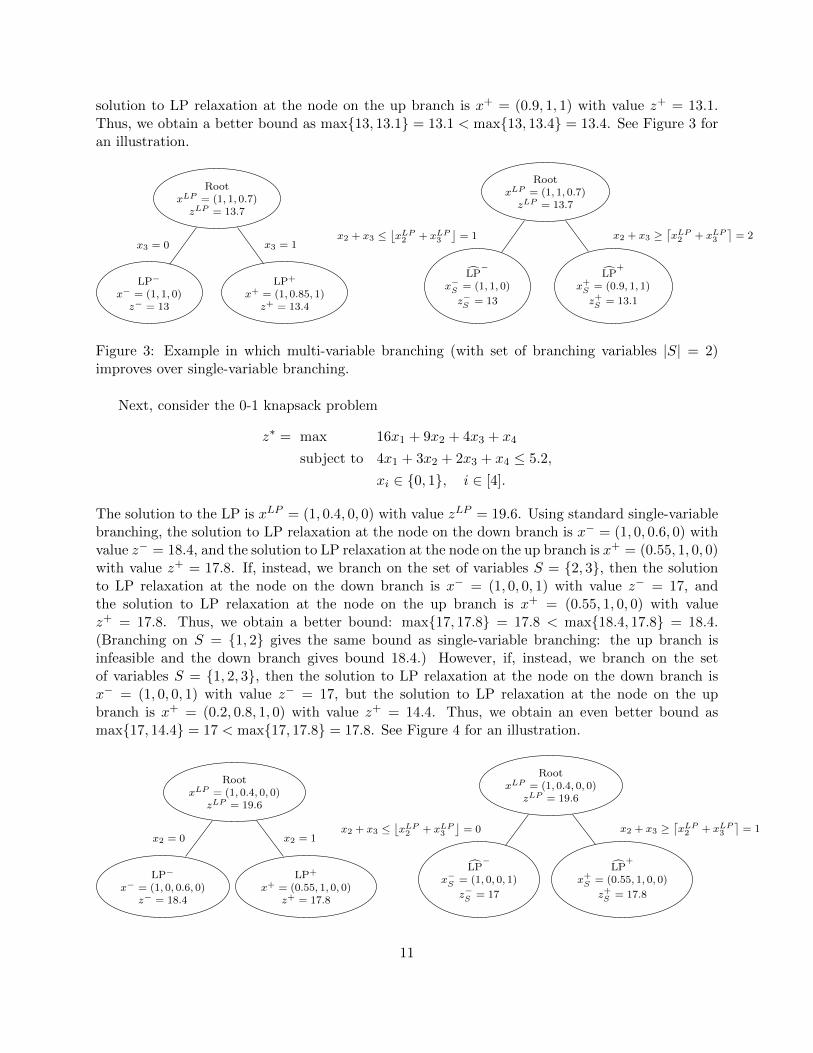
solution to LP relaxation at the node on the up branch is x+ = (0.9, 1, 1) with value z+ = 13.1.Thus, we obtain a better bound as max{13, 13.1} = 13.1 < max{13, 13.4} = 13.4. See Figure 3 foran illustration.

RootxLP = (1, 1, 0.7)

zLP = 13.7

LP−

x− = (1, 1, 0)z− = 13

x3 = 0

LP+

x+ = (1, 0.85, 1)z+ = 13.4

x3 = 1

RootxLP = (1, 1, 0.7)

zLP = 13.7

LP−

x−S = (1, 1, 0)

z−S = 13

x2 + x3 ≤⌊xLP2 + xLP

3

⌋= 1

LP+

x+S = (0.9, 1, 1)

z+S = 13.1

x2 + x3 ≥⌈xLP2 + xLP

3

⌉= 2

Figure 3: Example in which multi-variable branching (with set of branching variables |S| = 2)improves over single-variable branching.

Next, consider the 0-1 knapsack problem

z∗ = max 16x1 + 9x2 + 4x3 + x4

subject to 4x1 + 3x2 + 2x3 + x4 ≤ 5.2,

xi ∈ {0, 1}, i ∈ [4].

The solution to the LP is xLP = (1, 0.4, 0, 0) with value zLP = 19.6. Using standard single-variablebranching, the solution to LP relaxation at the node on the down branch is x− = (1, 0, 0.6, 0) withvalue z− = 18.4, and the solution to LP relaxation at the node on the up branch is x+ = (0.55, 1, 0, 0)with value z+ = 17.8. If, instead, we branch on the set of variables S = {2, 3}, then the solutionto LP relaxation at the node on the down branch is x− = (1, 0, 0, 1) with value z− = 17, andthe solution to LP relaxation at the node on the up branch is x+ = (0.55, 1, 0, 0) with valuez+ = 17.8. Thus, we obtain a better bound: max{17, 17.8} = 17.8 < max{18.4, 17.8} = 18.4.(Branching on S = {1, 2} gives the same bound as single-variable branching: the up branch isinfeasible and the down branch gives bound 18.4.) However, if, instead, we branch on the setof variables S = {1, 2, 3}, then the solution to LP relaxation at the node on the down branch isx− = (1, 0, 0, 1) with value z− = 17, but the solution to LP relaxation at the node on the upbranch is x+ = (0.2, 0.8, 1, 0) with value z+ = 14.4. Thus, we obtain an even better bound asmax{17, 14.4} = 17 < max{17, 17.8} = 17.8. See Figure 4 for an illustration.

RootxLP = (1, 0.4, 0, 0)

zLP = 19.6

LP−

x− = (1, 0, 0.6, 0)z− = 18.4

x2 = 0

LP+

x+ = (0.55, 1, 0, 0)z+ = 17.8

x2 = 1

RootxLP = (1, 0.4, 0, 0)

zLP = 19.6

LP−

x−S = (1, 0, 0, 1)

z−S = 17

x2 + x3 ≤⌊xLP2 + xLP

3

⌋= 0

LP+

x+S = (0.55, 1, 0, 0)

z+S = 17.8

x2 + x3 ≥⌈xLP2 + xLP

3

⌉= 1

11

RootxLP = (1, 0.4, 0, 0)

zLP = 19.6

LP−

x−S

= (1, 0, 0, 1)

z−S

= 17

x1 + x2 + x3 ≤⌊xLP1 + xLP

2 + xLP3

⌋= 1

LP+

x+

S= (0.2, 0.8, 1, 0)

z−S

= 14.4

x1 + x2 + x3 ≥⌈xLP1 + xLP

2 + xLP3

⌉= 2

Figure 4: Example in which multi-variable branching using a set of branching variables of size threeimproves over multi-variable branching using a set of branching variables of size two.

Next, we present a necessary, but not sufficient, condition as well as a sufficient, but notnecessary, condition for multi-variable branching using a set of variables of size two to outperformsingle-variable branching. In all that follows, when we say “outperforms” or “is better than” wemean that the dual bound after branching is lower. Without loss of generality, suppose p1

w1≥ p2

w2≥

. . . ≥ pnwn

and that the solution to the LP relaxation at the root node is fractional, i.e., the solutionhas the form

xLP = (1, . . . , 1︸ ︷︷ ︸i−1

, f, 0, . . . , 0︸ ︷︷ ︸n−i

),

with 1 < i ≤ n. (Note that we have assumed that wi ≤ b for i = 1, . . . , n.) We consider two cases,i = n and 1 < i < n− 1. In the former case, we give a necessary condition for branching on a setof two variables to outperform single-variable branching. In the latter case, we provide a sufficientcondition.

Proposition 2. If i = n, then branching on S = {k, n} can be better than branching on S′ = {n}only if the solution to the LP relaxation on the up branch, x+, is fractional and k is the index ofthe fractional variable in x+.

Proof. Since i = n, it must be that xLP = (1, 1, . . . , 1, f) with 0 < f < 1. It is easy to see thatbranching on S′ gives

x− = (1, . . . , 1︸ ︷︷ ︸n−1

, 0), x+ = (1, . . . , 1︸ ︷︷ ︸k−1

, f+, 0, . . . , 0︸ ︷︷ ︸n−k−1

, 1), 0 ≤ f+ ≤ 1, 1 ≤ k ≤ n− 1.

If f+ is integer, then we have integer solutions on both the down and the up branch, and z =max{z−, z+} is the optimal value for the original IP. Therefore, branching on S cannot be betterthan branching on S′.

So assume 0 < f+ < 1. Consider S = {`, n} with ` < k (k ≥ 2). On the down branch we addx` + xn ≤

⌊xLP` + xLPn

⌋= 1, and on the up branch we add x` + xn ≥

⌈xLP` + xLPn

⌉= 2. Note

that x− is feasible for the down branch, and, thus, z−S ≥ z−. Similarly, x+ is feasible for the upbranch, and, thus, z+S ≥ z+. This implies zS = max{z−S , z

+S } ≥ max{z−, z+} = z, which means that

branching on S cannot be better than branching on S′. Next, consider S = {`, n} with k < ` < n(k ≤ n− 2). On the down branch, we add x` + xn ≤

⌊xLP` + xLPn

⌋= 1, which is satisfied by both

x− and x+. Again, branching on S cannot be better than branching on S′. �

12

Proposition 3. Suppose 1 < i < n − 1 and let pi+1

wi+1> pi+2

wi+2and wi+1 ≥ wi. Furthermore, let

the value of the solution to the LP relaxation on the down branch be greater than the value of thesolution to the LP relaxation on the up branch, i.e., z− > z+, when branching on S′ = {i}. Thenbranching on S = {i, i+ 1} is better than branching on S′ and achieves the best bound that can beachieved by branching on a set of variables of size two.

Proof. Since wi+1 ≥ wi, branching on S′ results, on the down branch, in

x− = (1, . . . , 1︸ ︷︷ ︸i−1

, 0, f−, 0, . . . , 0︸ ︷︷ ︸n−i−2

), 0 < f− < 1.

When we branch on S, we add xi + xi+1 ≤⌊xLPi + xLPi+1

⌋= 0 on the down branch, and, because

pi+1

wi+1> pi+2

wi+2, we have that z−S < z−.

Let b = b−∑i−1

k=1wk. Because xLPi = f is fractional, wi > b, thus, wi+1 > b. We will show thatx+S = x+, and, thus, z+S = z+. When we branch on S, we add xi + xi+1 ≥ dxLPi + xLPi+1e = 1, whichcauses some “waste” of the resource as items i and (i+1) are less desirable than items 1 through i−1.By setting xi = 1 and xi+1 = 0, the branching constraint is satisfied and the waste is minimized.As a consequence, we obtain solution x+. Thus, zS = max{z−S , z

+S } = max{z−S , z+} < z− = z.

Next, consider branching on S′′ = {k, i} 6= {i, i + 1}. When k < i, we add xk + xi ≤⌊xLPk + xLPi

⌋= 1 on the down branch, and have z−S′′ ≥ z−, because x− satisfies x−k + x−i ≤ 1.

This implies z−S′′ ≥ z− > z+, i.e., branching on S′′ cannot be better than branching on S (in fact,it cannot even better than branching on S′). When k > i+ 1, we add xi + xk ≤

⌊xLPi + xLPk

⌋= 0

on the down branch, and have xi = xk = 0. Since wi+1 ≥ wi > b, all of the resource can beconsumed by items in {1, . . . , i− 1, i+ 1}. When branching on S, on the down branch only itemsin {1, . . . , i − 1, i + 2, . . . , n} can be used, which implies z−S′′ ≥ z−S . We have already argued thatwhen we branch on S, on the up branch we will have x+i = 1 and x+i+1 = 0. This solution is feasiblewhen branching on S′′, as xi + xk ≥

⌊xLPi + xLPk

⌋= 1 is added on the up branch. Therefore, we

also have z+S′′ ≥ z+S , which implies branching on S′′ cannot be better than branching on S. �

5 Computational Study

In this section, we evaluate the performance of four multi-variable branching schemes motivatedby the observations in the previous section.

5.1 Branching on sets of size two

The first two multi-variable branching schemes involve sets of size two in order to limit the com-putation time required to identify the set of variables to branch on. In the first scheme, which isinspired by the analysis in Section 4, we choose S = {i, i+ 1} where i is the largest index such thatx∗i is fractional and i < n, and choose S = {i, j}, when i = n and where j the largest index suchthat x∗j ∈ {0, 1}. Observe that this multi-variable branching scheme is attractive computationallyas determining S does not require the solution of any linear programs. We call this scheme “B1”.In the second scheme, we randomly select an additional set S of size two and branch on the setthat results in the best bound (i.e., either S or S). Observe that this scheme introduces diversifi-cation, which may improve its performance, but it comes at the price of having to solve four linearprograms. We call this scheme “B2”.

13

5.2 Branching on dynamically determined sets

The last two multi-variable branching schemes may involve sets of size larger than two as thismay improve the performance (as we have seen in Section 4). To control the computation timesomewhat, we generate the set S of variables to branch on dynamically. More specifically, westart from S = {i} with i the index of the fractional variable that gives the best bound among allfractional variables when branching on these variables. Note that i is the index of the variable thatwould be chosen if strong branching was used. Next, we evaluate sets S = {i, j} for j such thatxLPi + xLPj is fractional, and, again, choose the set that gives the best bound, say S = {i, j}. If

the best bound associated with {i, j} is smaller that the best bound associated with {i}, then theprocess continues, i.e., we explores all sets of size three, extending {i, j}, to see if there is one amongthem that results in a smaller best bound. We continue extending the set S with one more variableas long as it results in an improved bound. We call this scheme “B3”. Clearly, this branchingscheme is computationally intensive, and, therefore, we consider a variant in which the cardinalityof the set is limited to at most K1 and it is only applied at the top of the search tree, i.e., atnodes of depth less than or equal to K2. At nodes of depth more than K2, standard single-variablebranching is used, where we branch on the fractional variable with the smallest index. We call thisscheme “B4”.

5.3 Computational experiments

In our computational experiments, we compare the five branching schemes:

B0: Standard single-variable branching;

B1: Standard multi-variable branching on sets of size two;

B2: Enhanced multi-variable branching with sets of size two;

B3: Multi-variable branching with dynamically generated sets S; and

B4: Multi-variable branching with restricted dynamically generated sets S.

In branching scheme B4, we restrict the size of S to at most three and apply multi-variable branch-ing at nodes up to depth 10. We compare these five variable selection schemes using two nodeselection schemes: depth first search (DFS) and best first search (BFS).

The code is implemented in MATLAB (2018b) and uses the general branching and boundframework with our branching schemes. CPLEX 12.8 is used for solving the linear programs.All computational experiments were run on a 20-core machine with Intel(R) Xeon(R) 2.30GHzprocessors and 512GB of memory.

The instances are generated randomly, where p and w are integers chosen uniformly from

[M ] = {1, 2, . . . ,M}, and b =⌊∑n

i=1 wi

2

⌋. We test instances with n ∈ {50, 60, 70, 80, 90, 100},

and M ∈ {1000, 2000, 3000, 4000, 5000}, i.e., 30 different combinations of n and M . For eachcombination, we generate 100 instances, i.e., we use 3, 000 instances.

The performance metrics of interest are: (1) N : the number of nodes evaluated, (2) t1: thesolve time, (3) t2: the average node solve time, and (4) t3: the average time per node spent onfinding the set of variables to branch on.

14

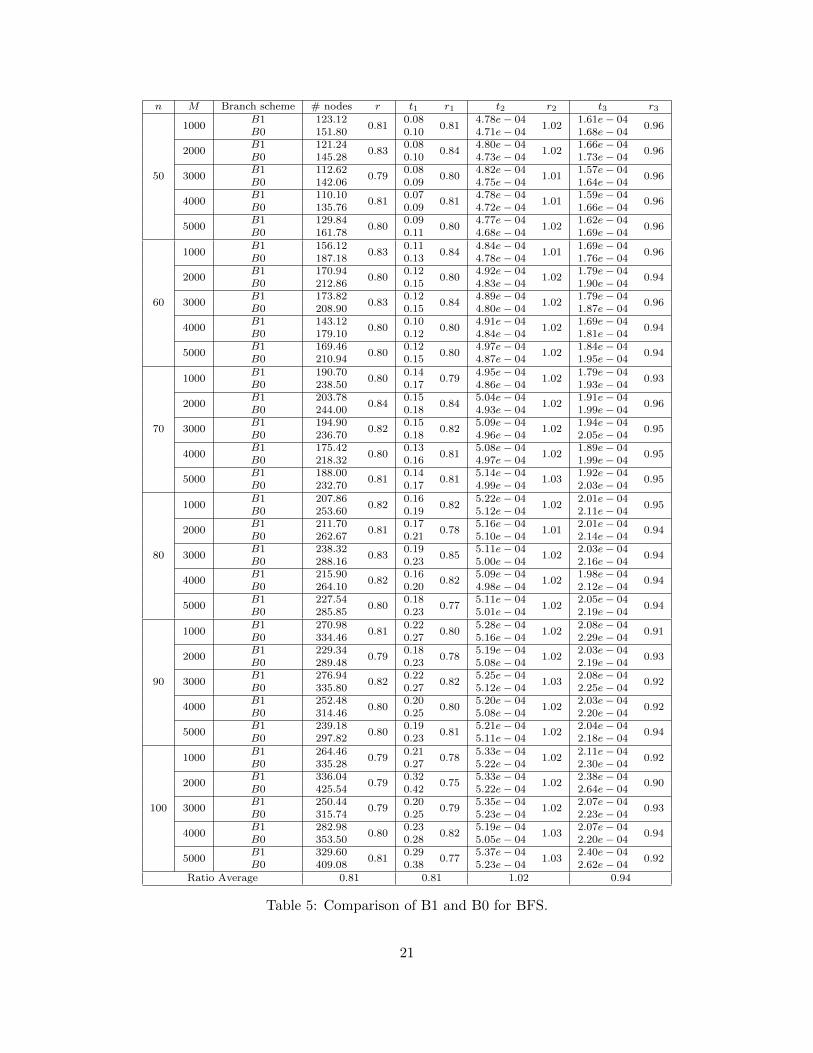
In Figure 5, we plot the performance profile (Dolan and More 2002) when using the five branch-ing schemes with respect to N , the number of nodes evaluated, for DFS and BFS, and in Figure 6,we plot the performance profile when using the five branching schemes with respect to t1, the solvetime, for DFS and BFS. In Table 1, we report, for each of the branching schemes, the number ofnodes evaluated and the solve time as a fraction of the number of nodes evaluated and the solvetime of standard single-variable branching, respectively, average over all instances. In Tables 2 and3, we report the values of t2 and t3 averaged over instances of the same size. Detailed comparisonsof the results for all instances can be found in the appendix.

0 1 2 3 4 5 6 7 8

log( )

0

0.1

0.2

0.3

0.4

0.5

0.6

0.7

0.8

0.9

1

P(r

p,s

log(

) :1

s n

s)

Number of nodes explored (DFS)

B0

B1

B2

B3

B4

0 1 2 3 4 5

log( )

0

0.1

0.2

0.3

0.4

0.5

0.6

0.7

0.8

0.9

1

P(r

p,s

log(

) :1

s n

s)

Number of nodes explored (BFS)

B0

B1

B2

B3

B4

Figure 5: Performance profile on number of nodes explored N .

0 1 2 3 4 5 6 7 8 9

log( )

0

0.1

0.2

0.3

0.4

0.5

0.6

0.7

0.8

0.9

1

P(r

p,s

log(

) :1

s n

s)

Total time (DFS)

B0

B1

B2

B3

B4

0 1 2 3 4 5 6 7 8 9

log( )

0

0.1

0.2

0.3

0.4

0.5

0.6

0.7

0.8

0.9

1

P(r

p,s

log(

) :1

s n

s)

Total time (BFS)

B0

B1

B2

B3

B4

Figure 6: Performance profile on total running time t1.

Figure 5 shows (and so does Table 1) that all four multi-variable branching schemes achievebetter node-efficiency than standard single-variable branching for both DFS and BFS. Furthermore,it is also clear that branching scheme B3 results in the most significant reduction in number of nodesevaluated. However, Figure 6 reveals (and so does Table 1) that this reduction in number of nodesevaluated comes at a high price in terms of solve time. In fact, Figure 6 shows that only branchingscheme B1 reduces solve time, and that the reduction is more pronounced for BFS. The results

15

DFS BFSB0 B1 B2 B3 B4 B0 B1 B2 B3 B4

N 1.00 0.80 0.77 0.13 0.76 1.00 0.81 0.72 0.13 0.47

t1 1.00 0.83 1.85 87.83 14.64 1.00 0.80 2.50 74.89 44.56

Table 1: Ratios of N and t1 with respect to B0.

DFS BFS

n B0 B1 B2 B3 B4 B0 B1 B2 B3 B4

50 4.61 4.80 4.89 5.01 4.85 4.72 4.79 4.89 4.62 4.79

60 4.74 4.92 5.03 5.13 4.96 4.82 4.91 5.01 4.73 4.91

70 4.87 5.08 5.15 5.27 5.07 4.94 5.06 5.14 4.86 5.03

80 4.96 5.15 5.23 5.38 5.17 5.04 5.14 5.23 4.97 5.12

90 5.02 5.23 5.29 5.43 5.23 5.11 5.23 5.30 5.05 5.19

100 5.12 5.33 5.38 5.50 5.30 5.19 5.31 5.39 5.11 5.27

Table 2: Average time per node spent on solving the node t2 (×10−4).

DFS BFS

n B0 B1 B2 B3 B4 B0 B1 B2 B3 B4

50 0.59 0.60 7.05 1612.92 116.36 1.68 1.61 17.72 2111.13 727.28

60 0.60 0.60 7.43 2257.80 115.21 1.86 1.76 18.91 2959.84 818.00

70 0.61 0.62 7.84 2999.57 110.79 2.00 1.89 20.20 3765.11 880.18

80 0.64 0.78 8.17 3883.02 110.58 2.14 2.02 21.06 4949.34 882.37

90 0.62 0.62 8.38 4800.76 110.17 2.22 2.05 21.60 6023.86 870.65

100 0.63 0.64 8.90 5822.69 107.47 2.40 2.21 23.07 7276.84 891.02

Table 3: Average time per node spent on finding the set of variables to branch on t3 (×10−4).

16

for branching scheme B1 in Table 1 clear indicate the promise of multi-variable branching, boththe number of nodes and the solve time are reduced. As expected, branching scheme B4 is fasterthan branching scheme B3 even though it explores many more nodes. Tuning the two restrictionparameters of B4 may achieve an even better balance between node-efficiency and time-efficiency.Tables 2 and 3 show that the difficulty of the subproblems created by the different branchingschemes is nearly the same and the increase in solve time is mostly due to finding the sets ofvariables to branch on.

6 Final Remarks

In this paper, we explored the potential benefits of branching on sets of variables rather thanstandard single-variable branching. Preliminary computational experiments on randomly generatedinstances of the 0-1 knapsack problem show promise and reveal the trade off between node-efficiencyand time-efficiency. Our current research is focused on reproducing the promise of multi-variablebranching on general mixed integer programs and developing efficient heuristics to obtain high-quality sets of variables to branch on.

Acknowledgment

We want to thank Andrea Lodi for reading an earlier version of the paper and providing valuablecomments and suggestions.

References

K. Aardal, R. Weismantel, and L. A. Wolsey. Non-standard approaches to integer programming. DiscreteApplied Mathematics, 123(1):5 – 74, 2002.

T. Achterberg. Constraint integer programming. 2007.

T. Achterberg, T. Koch, and A. Martin. Branching rules revisited. Operations Research Letters, 33(1):42–54,2005.

D. Applegate, R. Bixby, V. Chvatal, and B. Cook. Finding cuts in the tsp (a preliminary report). Technicalreport, Center for Discrete Mathematics & Theoretical Computer Science, 1995.

E. Beale. Branch and bound methods for mathematical programming systems. In P. Hammer, E. Johnson,and B. Korte, editors, Discrete Optimization II, volume 5 of Annals of Discrete Mathematics, pages201 – 219. Elsevier, 1979.

E. M. L. Beale and J. A. Tomlin. Special facilities in a general mathematical programming system fornon-convex problems using ordered sets of variables. In J. Lawrence, editor, Proceedings 5th IFORSConference, Tavistock, pages 447–454. Wiley, 1970.

M. Benichou, J.-M. Gauthier, P. Girodet, G. Hentges, G. Ribiere, and O. Vincent. Experiments in mixed-integer linear programming. Mathematical Programming, 1(1):76–94, 1971.

V. Chvatal. Hard knapsack problems. Operations Research, 28(6):1402–1411, 1980.

G. Di Liberto, S. Kadioglu, K. Leo, and Y. Malitsky. Dash: Dynamic approach for switching heuristics.European Journal of Operational Research, 248(3):943–953, 2016.

E. D. Dolan and J. J. More. Benchmarking Optimization Software with Performance Profiles. MathematicalProgramming, 91:201–213, 2002.

17

J.-M. Gauthier and G. Ribiere. Experiments in mixed-integer linear programming using pseudo-costs. Math-ematical Programming, 12(1):26–47, 1977.

E. B. Khalil, P. Le Bodic, L. Song, G. L. Nemhauser, and B. N. Dilkina. Learning to branch in mixed integerprogramming. In AAAI, pages 724–731, 2016.

B. Krishnamoorthy and G. Pataki. Column basis reduction and decomposable knapsack problems. DiscreteOptimization, 6(3):242 – 270, 2009.

A. H. Land and A. G. Doig. An automatic method of solving discrete programming problems. Econometrica:Journal of the Econometric Society, pages 497–520, 1960.

H. Lenstra, Jr. Integer programming with a fixed number of variables. Mathematics of Operations Research,8:538––548, 1983.

J. T. Linderoth and M. W. Savelsbergh. A computational study of search strategies for mixed integerprogramming. INFORMS Journal on Computing, 11(2):173–187, 1999.

A. Lodi and G. Zarpellon. On learning and branching: a survey. Top, 25(2):207–236, 2017.

A. Marcos Alvarez, L. Wehenkel, and Q. Louveaux. Online learning for strong branching approximation inbranch-and-bound. Technical report, University of Liege, 2016.

A. Marcos Alvarez, Q. Louveaux, and L. Wehenkel. A machine learning-based approximation of strongbranching. INFORMS Journal on Computing, 29(1):185–195, 2017.

D. R. Morrison, S. H. Jacobson, J. J. Sauppe, and E. C. Sewell. Branch-and-bound algorithms: A survey ofrecent advances in searching, branching, and pruning. Discrete Optimization, 19:79 – 102, 2016. ISSN1572-5286.

G. Pataki and M. Tural. Basis reduction methods. In J. J. Cochran, L. A. Cox Jr., P. Keskinocak, J. P.Kharoufeh, and J. C. Smith, editors, Wiley Encyclopedia of Operations Research and ManagementScience. 2011.

18

Appendix. Detailed results of experiments

19

n M Branch scheme # nodes r t1 r1 t2 r2 t3 r3

50

1000B1 647.70

0.780.35

0.814.78e− 04

1.046.07e− 05

1.01B0 833.86 0.43 4.59e− 04 6.01e− 05

2000B1 721.22

0.790.39

0.824.79e− 04

1.046.01e− 05

1.00B0 911.66 0.48 4.60e− 04 5.99e− 05

3000B1 660.10

0.770.36

0.804.80e− 04

1.035.97e− 05

1.02B0 853.94 0.45 4.64e− 04 5.88e− 05

4000B1 636.32

0.780.35

0.824.84e− 04

1.046.09e− 05

1.02B0 813.28 0.42 4.64e− 04 5.99e− 05

5000B1 695.02

0.810.37

0.844.78e− 04

1.045.89e− 05

1.03B0 859.42 0.44 4.57e− 04 5.72e− 05

60

1000B1 863.04

0.770.47

0.804.86e− 04

1.055.93e− 05

1.03B0 1124.46 0.59 4.65e− 04 5.74e− 05

2000B1 885.82

0.790.49

0.824.92e− 04

1.046.06e− 05

1.01B0 1116.16 0.60 4.74e− 04 6.01e− 05

3000B1 1002.44

0.810.55

0.844.91e− 04

1.045.97e− 05

1.02B0 1235.38 0.66 4.74e− 04 5.88e− 05

4000B1 858.58

0.780.48

0.804.92e− 04

1.046.08e− 05

1.01B0 1104.40 0.59 4.75e− 04 6.01e− 05

5000B1 967.42

0.800.54

0.824.97e− 04

1.036.10e− 05

1.00B0 1214.78 0.66 4.82e− 04 6.11e− 05

70

1000B1 1199.24

0.800.67

0.845.00e− 04

1.055.93e− 05

1.02B0 1496.92 0.80 4.77e− 04 5.83e− 05

2000B1 1220.20

0.770.69

0.805.07e− 04

1.046.05e− 05

1.02B0 1582.12 0.86 4.86e− 04 5.95e− 05

3000B1 1173.46

0.760.67

0.795.09e− 04

1.046.25e− 05

1.02B0 1543.20 0.85 4.88e− 04 6.12e− 05

4000B1 1158.78

0.820.67

0.855.09e− 04

1.036.31e− 05

1.01B0 1411.46 0.79 4.93e− 04 6.23e− 05

5000B1 1122.30

0.790.65

0.835.15e− 04

1.056.36e− 05

1.04B0 1418.14 0.78 4.92e− 04 6.14e− 05

80

1000B1 1372.80

0.830.81

0.865.23e− 04

1.046.40e− 05

1.01B0 1657.60 0.94 5.03e− 04 6.32e− 05

2000B1 1400.14

0.780.82

0.805.20e− 04

1.041.24e− 04

1.91B0 1804.64 1.02 5.02e− 04 6.52e− 05

3000B1 1471.98

0.830.85

0.865.13e− 04

1.046.11e− 05

1.00B0 1780.04 0.99 4.94e− 04 6.14e− 05

4000B1 1242.04

0.820.71

0.855.08e− 04

1.046.22e− 05

0.99B0 1512.00 0.83 4.87e− 04 6.25e− 05

5000B1 1462.14

0.870.84

0.905.10e− 04

1.047.75e− 05

1.15B0 1681.48 0.93 4.92e− 04 6.72e− 05

90

1000B1 1629.00

0.780.96

0.815.28e− 04

1.046.22e− 05

1.02B0 2101.26 1.19 5.05e− 04 6.11e− 05

2000B1 1661.18

0.820.98

0.855.22e− 04

1.046.26e− 05

1.01B0 2036.98 1.15 5.02e− 04 6.20e− 05

3000B1 1571.30

0.810.92

0.855.23e− 04

1.046.24e− 05

1.02B0 1933.46 1.09 5.01e− 04 6.14e− 05

4000B1 1608.46

0.790.94

0.825.21e− 04

1.046.17e− 05

1.01B0 2046.06 1.15 5.00e− 04 6.09e− 05

5000B1 1674.62

0.840.98

0.875.22e− 04

1.046.30e− 05

1.00B0 2000.22 1.13 5.01e− 04 6.28e− 05

100

1000B1 1938.66

0.821.17

0.865.38e− 04

1.046.46e− 05

1.02B0 2349.94 1.36 5.16e− 04 6.36e− 05

2000B1 1948.24

0.811.17

0.845.36e− 04

1.046.40e− 05

1.01B0 2417.12 1.40 5.15e− 04 6.36e− 05

3000B1 1847.44

0.791.11

0.825.36e− 04

1.046.38e− 05

1.01B0 2333.88 1.35 5.14e− 04 6.29e− 05

4000B1 1879.08

0.791.09

0.825.18e− 04

1.046.04e− 05

1.00B0 2389.72 1.33 4.97e− 04 6.01e− 05

5000B1 1962.90

0.801.19

0.835.37e− 04

1.046.65e− 05

1.02B0 2445.20 1.43 5.17e− 04 6.55e− 05

Ratio Average 0.80 0.83 1.04 1.05

Table 4: Comparison of B1 and B0 for DFS.

20

n M Branch scheme # nodes r t1 r1 t2 r2 t3 r3

50

1000B1 123.12

0.810.08

0.814.78e− 04

1.021.61e− 04

0.96B0 151.80 0.10 4.71e− 04 1.68e− 04

2000B1 121.24

0.830.08

0.844.80e− 04

1.021.66e− 04

0.96B0 145.28 0.10 4.73e− 04 1.73e− 04

3000B1 112.62

0.790.08

0.804.82e− 04

1.011.57e− 04

0.96B0 142.06 0.09 4.75e− 04 1.64e− 04

4000B1 110.10

0.810.07

0.814.78e− 04

1.011.59e− 04

0.96B0 135.76 0.09 4.72e− 04 1.66e− 04

5000B1 129.84

0.800.09

0.804.77e− 04

1.021.62e− 04

0.96B0 161.78 0.11 4.68e− 04 1.69e− 04

60

1000B1 156.12

0.830.11

0.844.84e− 04

1.011.69e− 04

0.96B0 187.18 0.13 4.78e− 04 1.76e− 04

2000B1 170.94

0.800.12

0.804.92e− 04

1.021.79e− 04

0.94B0 212.86 0.15 4.83e− 04 1.90e− 04

3000B1 173.82

0.830.12

0.844.89e− 04

1.021.79e− 04

0.96B0 208.90 0.15 4.80e− 04 1.87e− 04

4000B1 143.12

0.800.10

0.804.91e− 04

1.021.69e− 04

0.94B0 179.10 0.12 4.84e− 04 1.81e− 04

5000B1 169.46

0.800.12

0.804.97e− 04

1.021.84e− 04

0.94B0 210.94 0.15 4.87e− 04 1.95e− 04

70

1000B1 190.70

0.800.14

0.794.95e− 04

1.021.79e− 04

0.93B0 238.50 0.17 4.86e− 04 1.93e− 04

2000B1 203.78

0.840.15

0.845.04e− 04

1.021.91e− 04

0.96B0 244.00 0.18 4.93e− 04 1.99e− 04

3000B1 194.90

0.820.15

0.825.09e− 04

1.021.94e− 04

0.95B0 236.70 0.18 4.96e− 04 2.05e− 04

4000B1 175.42

0.800.13

0.815.08e− 04

1.021.89e− 04

0.95B0 218.32 0.16 4.97e− 04 1.99e− 04

5000B1 188.00

0.810.14

0.815.14e− 04

1.031.92e− 04

0.95B0 232.70 0.17 4.99e− 04 2.03e− 04

80

1000B1 207.86

0.820.16

0.825.22e− 04

1.022.01e− 04

0.95B0 253.60 0.19 5.12e− 04 2.11e− 04

2000B1 211.70

0.810.17

0.785.16e− 04

1.012.01e− 04

0.94B0 262.67 0.21 5.10e− 04 2.14e− 04

3000B1 238.32

0.830.19

0.855.11e− 04

1.022.03e− 04

0.94B0 288.16 0.23 5.00e− 04 2.16e− 04

4000B1 215.90

0.820.16

0.825.09e− 04

1.021.98e− 04

0.94B0 264.10 0.20 4.98e− 04 2.12e− 04

5000B1 227.54

0.800.18

0.775.11e− 04

1.022.05e− 04

0.94B0 285.85 0.23 5.01e− 04 2.19e− 04

90

1000B1 270.98

0.810.22

0.805.28e− 04

1.022.08e− 04

0.91B0 334.46 0.27 5.16e− 04 2.29e− 04

2000B1 229.34

0.790.18

0.785.19e− 04

1.022.03e− 04

0.93B0 289.48 0.23 5.08e− 04 2.19e− 04

3000B1 276.94

0.820.22

0.825.25e− 04

1.032.08e− 04

0.92B0 335.80 0.27 5.12e− 04 2.25e− 04

4000B1 252.48

0.800.20

0.805.20e− 04

1.022.03e− 04

0.92B0 314.46 0.25 5.08e− 04 2.20e− 04

5000B1 239.18

0.800.19

0.815.21e− 04

1.022.04e− 04

0.94B0 297.82 0.23 5.11e− 04 2.18e− 04

100

1000B1 264.46

0.790.21

0.785.33e− 04

1.022.11e− 04

0.92B0 335.28 0.27 5.22e− 04 2.30e− 04

2000B1 336.04

0.790.32

0.755.33e− 04

1.022.38e− 04

0.90B0 425.54 0.42 5.22e− 04 2.64e− 04

3000B1 250.44

0.790.20

0.795.35e− 04

1.022.07e− 04

0.93B0 315.74 0.25 5.23e− 04 2.23e− 04

4000B1 282.98

0.800.23

0.825.19e− 04

1.032.07e− 04

0.94B0 353.50 0.28 5.05e− 04 2.20e− 04

5000B1 329.60

0.810.29

0.775.37e− 04

1.032.40e− 04

0.92B0 409.08 0.38 5.23e− 04 2.62e− 04

Ratio Average 0.81 0.81 1.02 0.94

Table 5: Comparison of B1 and B0 for BFS.

21

n M Branch scheme # nodes r t1 r1 t2 r2 t3 r3

50

1000B2 627.90

0.750.75

1.734.90e− 04

1.077.01e− 04

11.65B0 833.86 0.43 4.59e− 04 6.01e− 05

2000B2 719.06

0.790.88

1.854.89e− 04

1.067.27e− 04

12.14B0 911.66 0.48 4.60e− 04 5.99e− 05

3000B2 618.56

0.720.74

1.664.94e− 04

1.067.11e− 04

12.10B0 853.94 0.45 4.64e− 04 5.88e− 05

4000B2 613.56

0.750.73

1.724.87e− 04

1.056.96e− 04

11.62B0 813.28 0.42 4.64e− 04 5.99e− 05

5000B2 651.34

0.760.77

1.744.85e− 04

1.066.92e− 04

12.11B0 859.42 0.44 4.57e− 04 5.72e− 05

60

1000B2 832.20

0.741.01

1.724.95e− 04

1.077.19e− 04

12.53B0 1124.46 0.59 4.65e− 04 5.74e− 05

2000B2 857.66

0.771.07

1.795.04e− 04

1.067.43e− 04

12.36B0 1116.16 0.60 4.74e− 04 6.01e− 05

3000B2 880.88

0.711.09

1.664.99e− 04

1.057.40e− 04

12.58B0 1235.38 0.66 4.74e− 04 5.88e− 05

4000B2 846.06

0.771.07

1.805.07e− 04

1.077.51e− 04

12.49B0 1104.40 0.59 4.75e− 04 6.01e− 05

5000B2 874.26

0.721.12

1.695.11e− 04

1.067.64e− 04

12.49B0 1214.78 0.66 4.82e− 04 6.11e− 05

70

1000B2 1177.76

0.791.49

1.865.07e− 04

1.067.57e− 04

12.99B0 1496.92 0.80 4.77e− 04 5.83e− 05

2000B2 1175.82

0.741.51

1.755.14e− 04

1.067.68e− 04

12.92B0 1582.12 0.86 4.86e− 04 5.95e− 05

3000B2 1136.54

0.741.49

1.765.17e− 04

1.067.91e− 04

12.93B0 1543.20 0.85 4.88e− 04 6.12e− 05

4000B2 1065.88

0.761.41

1.795.17e− 04

1.057.99e− 04

12.81B0 1411.46 0.79 4.93e− 04 6.23e− 05

5000B2 1014.06

0.721.34

1.715.19e− 04

1.068.05e− 04

13.11B0 1418.14 0.78 4.92e− 04 6.14e− 05

80

1000B2 1319.68

0.801.84

1.965.32e− 04

1.068.60e− 04

13.60B0 1657.60 0.94 5.03e− 04 6.32e− 05

2000B2 1361.74

0.751.84

1.815.29e− 04

1.058.05e− 04

12.34B0 1804.64 1.02 5.02e− 04 6.52e− 05

3000B2 1409.72

0.791.86

1.885.19e− 04

1.057.97e− 04

12.98B0 1780.04 0.99 4.94e− 04 6.14e− 05

4000B2 1260.00

0.831.66

1.995.17e− 04

1.067.95e− 04

12.72B0 1512.00 0.83 4.87e− 04 6.25e− 05

5000B2 1367.18

0.811.86

2.005.19e− 04

1.058.28e− 04

12.31B0 1681.48 0.93 4.92e− 04 6.72e− 05

90

1000B2 1652.10

0.792.31

1.935.33e− 04

1.058.53e− 04

13.96B0 2101.26 1.19 5.05e− 04 6.11e− 05

2000B2 1617.90

0.792.21

1.925.29e− 04

1.058.33e− 04

13.44B0 2036.98 1.15 5.02e− 04 6.20e− 05

3000B2 1519.58

0.792.08

1.905.28e− 04

1.058.35e− 04

13.60B0 1933.46 1.09 5.01e− 04 6.14e− 05

4000B2 1524.64

0.752.07

1.805.28e− 04

1.058.24e− 04

13.53B0 2046.06 1.15 5.00e− 04 6.09e− 05

5000B2 1541.24

0.772.13

1.885.30e− 04

1.068.43e− 04

13.43B0 2000.22 1.13 5.01e− 04 6.28e− 05

100

1000B2 1778.64

0.762.58

1.895.42e− 04

1.059.02e− 04

14.18B0 2349.94 1.36 5.16e− 04 6.36e− 05

2000B2 1833.74

0.762.63

1.885.41e− 04

1.058.88e− 04

13.96B0 2417.12 1.40 5.15e− 04 6.36e− 05

3000B2 1758.74

0.752.53

1.885.41e− 04

1.059.00e− 04

14.31B0 2333.88 1.35 5.14e− 04 6.29e− 05

4000B2 1860.04

0.782.54

1.915.24e− 04

1.058.41e− 04

13.99B0 2389.72 1.33 4.97e− 04 6.01e− 05

5000B2 1874.88

0.772.74

1.925.42e− 04

1.059.17e− 04

14.02B0 2445.20 1.43 5.17e− 04 6.55e− 05

Ratio Average 0.76 1.83 1.06 12.97

Table 6: Comparison of B2 and B0 for DFS.

22

n M Branch scheme # nodes r t1 r1 t2 r2 t3 r3

50

1000B2 110.06

0.730.25

2.494.88e− 04

1.041.73e− 03

10.32B0 151.80 0.10 4.71e− 04 1.68e− 04

2000B2 106.30

0.730.25

2.604.90e− 04

1.041.84e− 03

10.63B0 145.28 0.10 4.73e− 04 1.73e− 04

3000B2 101.90

0.720.23

2.444.91e− 04

1.031.76e− 03

10.72B0 142.06 0.09 4.75e− 04 1.64e− 04

4000B2 98.30

0.720.23

2.544.90e− 04

1.041.77e− 03

10.64B0 135.76 0.09 4.72e− 04 1.66e− 04

5000B2 116.04

0.720.26

2.424.87e− 04

1.041.76e− 03

10.40B0 161.78 0.11 4.68e− 04 1.69e− 04

60

1000B2 136.90

0.730.33

2.564.94e− 04

1.041.84e− 03

10.45B0 187.18 0.13 4.78e− 04 1.76e− 04

2000B2 154.08

0.720.37

2.485.01e− 04

1.041.89e− 03

9.92B0 212.86 0.15 4.83e− 04 1.90e− 04

3000B2 151.02

0.720.37

2.514.99e− 04

1.041.90e− 03

10.15B0 208.90 0.15 4.80e− 04 1.87e− 04

4000B2 129.62

0.720.32

2.545.04e− 04

1.041.89e− 03

10.47B0 179.10 0.12 4.84e− 04 1.81e− 04

5000B2 153.02

0.730.38

2.525.07e− 04

1.041.95e− 03

9.98B0 210.94 0.15 4.87e− 04 1.95e− 04

70

1000B2 172.20

0.720.43

2.475.04e− 04

1.041.92e− 03

9.95B0 238.50 0.17 4.86e− 04 1.93e− 04

2000B2 177.32

0.730.45

2.495.13e− 04

1.041.99e− 03

10.01B0 244.00 0.18 4.93e− 04 1.99e− 04

3000B2 174.74

0.740.46

2.605.17e− 04

1.042.06e− 03

10.04B0 236.70 0.18 4.96e− 04 2.05e− 04

4000B2 156.62

0.720.41

2.565.17e− 04

1.042.06e− 03

10.35B0 218.32 0.16 4.97e− 04 1.99e− 04

5000B2 167.26

0.720.44

2.535.20e− 04

1.042.07e− 03

10.23B0 232.70 0.17 4.99e− 04 2.03e− 04

80

1000B2 181.58

0.720.50

2.565.32e− 04

1.042.18e− 03

10.34B0 253.60 0.19 5.12e− 04 2.11e− 04

2000B2 190.86

0.730.52

2.435.26e− 04

1.032.07e− 03

9.65B0 262.67 0.21 5.10e− 04 2.14e− 04

3000B2 210.26

0.730.57

2.515.19e− 04

1.042.07e− 03

9.59B0 288.16 0.23 5.00e− 04 2.16e− 04

4000B2 195.32

0.740.52

2.585.19e− 04

1.042.07e− 03

9.76B0 264.10 0.20 4.98e− 04 2.12e− 04

5000B2 207.70

0.730.58

2.525.19e− 04

1.042.14e− 03

9.78B0 285.85 0.23 5.01e− 04 2.19e− 04

90

1000B2 245.04

0.730.66

2.425.34e− 04

1.032.17e− 03

9.46B0 334.46 0.27 5.16e− 04 2.29e− 04

2000B2 208.50

0.720.58

2.565.28e− 04

1.042.17e− 03

9.92B0 289.48 0.23 5.08e− 04 2.19e− 04

3000B2 247.70

0.740.67

2.525.28e− 04

1.032.13e− 03

9.46B0 335.80 0.27 5.12e− 04 2.25e− 04

4000B2 225.00

0.720.62

2.515.29e− 04

1.042.15e− 03

9.78B0 314.46 0.25 5.08e− 04 2.20e− 04

5000B2 217.52

0.730.61

2.615.30e− 04

1.042.18e− 03

10.00B0 297.82 0.23 5.11e− 04 2.18e− 04

100

1000B2 242.18

0.720.70

2.575.41e− 04

1.042.30e− 03

10.01B0 335.28 0.27 5.22e− 04 2.30e− 04

2000B2 303.60

0.710.93

2.205.42e− 04

1.042.33e− 03

8.83B0 425.54 0.42 5.22e− 04 2.64e− 04

3000B2 227.08

0.720.66

2.615.42e− 04

1.042.32e− 03

10.37B0 315.74 0.25 5.23e− 04 2.23e− 04

4000B2 251.94

0.710.71

2.565.25e− 04

1.042.18e− 03

9.88B0 353.50 0.28 5.05e− 04 2.20e− 04

5000B2 296.30

0.720.91

2.425.45e− 04

1.042.41e− 03

9.17B0 409.08 0.38 5.23e− 04 2.62e− 04

Ratio Average 0.72 2.51 1.04 10.01

Table 7: Comparison of B2 and B0 for BFS.

23

n M Branch scheme # nodes r t1 r1 t2 r2 t3 r3

50

1000B3 137.64

0.1721.87

50.504.98e− 04

1.091.61e− 01

2673.51B0 833.86 0.43 4.59e− 04 6.01e− 05

2000B3 155.69

0.1724.39

51.185.04e− 04

1.101.58e− 01

2645.22B0 911.66 0.48 4.60e− 04 5.99e− 05

3000B3 151.81

0.1824.44

54.895.05e− 04

1.091.63e− 01

2772.37B0 853.94 0.45 4.64e− 04 5.88e− 05

4000B3 148.24

0.1823.57

55.475.01e− 04

1.081.62e− 01

2703.09B0 813.28 0.42 4.64e− 04 5.99e− 05

5000B3 146.15

0.1723.44

52.894.98e− 04

1.091.63e− 01

2843.00B0 859.42 0.44 4.57e− 04 5.72e− 05

60

1000B3 165.06

0.1536.63

62.195.06e− 04

1.092.25e− 01

3916.80B0 1124.46 0.59 4.65e− 04 5.74e− 05

2000B3 164.78

0.1536.77

61.355.13e− 04

1.082.25e− 01

3744.16B0 1116.16 0.60 4.74e− 04 6.01e− 05

3000B3 174.32

0.1439.20

59.625.11e− 04

1.082.29e− 01

3890.02B0 1235.38 0.66 4.74e− 04 5.88e− 05

4000B3 185.92

0.1741.38

69.965.14e− 04

1.082.24e− 01

3725.29B0 1104.40 0.59 4.75e− 04 6.01e− 05

5000B3 183.99

0.1541.11

62.045.20e− 04

1.082.26e− 01

3698.25B0 1214.78 0.66 4.82e− 04 6.11e− 05

70

1000B3 211.23

0.1460.98

76.045.17e− 04

1.092.91e− 01

4995.42B0 1496.92 0.80 4.77e− 04 5.83e− 05

2000B3 208.66

0.1362.08

71.805.26e− 04

1.083.02e− 01

5075.66B0 1582.12 0.86 4.86e− 04 5.95e− 05

3000B3 210.49

0.1462.21

73.465.30e− 04

1.082.98e− 01

4866.50B0 1543.20 0.85 4.88e− 04 6.12e− 05

4000B3 208.76

0.1563.71

81.155.32e− 04

1.083.07e− 01

4931.97B0 1411.46 0.79 4.93e− 04 6.23e− 05

5000B3 210.56

0.1562.74

79.985.31e− 04

1.083.02e− 01

4916.35B0 1418.14 0.78 4.92e− 04 6.14e− 05

80

1000B3 228.33

0.1487.87

93.395.46e− 04

1.093.95e− 01

6251.55B0 1657.60 0.94 5.03e− 04 6.32e− 05

2000B3 224.55

0.1286.66

85.105.44e− 04

1.083.92e− 01

6017.34B0 1804.64 1.02 5.02e− 04 6.52e− 05

3000B3 232.15

0.1387.38

88.335.34e− 04

1.083.83e− 01

6243.50B0 1780.04 0.99 4.94e− 04 6.14e− 05

4000B3 208.58

0.1480.33

96.515.31e− 04

1.093.91e− 01

6255.30B0 1512.00 0.83 4.87e− 04 6.25e− 05

5000B3 229.36

0.1486.86

93.375.34e− 04

1.083.79e− 01

5640.63B0 1681.48 0.93 4.92e− 04 6.72e− 05

90

1000B3 245.28

0.12115.52

96.755.47e− 04

1.084.77e− 01

7812.44B0 2101.26 1.19 5.05e− 04 6.11e− 05

2000B3 234.79

0.12111.94

97.275.40e− 04

1.084.83e− 01

7795.34B0 2036.98 1.15 5.02e− 04 6.20e− 05

3000B3 218.09

0.11103.12

94.625.42e− 04

1.084.81e− 01

7844.70B0 1933.46 1.09 5.01e− 04 6.14e− 05

4000B3 246.00

0.12114.91

99.905.42e− 04

1.084.77e− 01

7824.09B0 2046.06 1.15 5.00e− 04 6.09e− 05

5000B3 242.12

0.12116.12

102.785.41e− 04

1.084.82e− 01

7677.26B0 2000.22 1.13 5.01e− 04 6.28e− 05

100

1000B3 249.50

0.11143.12

105.225.55e− 04

1.085.79e− 01

9108.26B0 2349.94 1.36 5.16e− 04 6.36e− 05

2000B3 258.22

0.11148.59

106.315.51e− 04

1.075.87e− 01

9216.85B0 2417.12 1.40 5.15e− 04 6.36e− 05

3000B3 262.26

0.11150.25

111.705.56e− 04

1.085.83e− 01

9281.03B0 2333.88 1.35 5.14e− 04 6.29e− 05

4000B3 254.49

0.11143.73

107.825.35e− 04

1.085.67e− 01

9433.55B0 2389.72 1.33 4.97e− 04 6.01e− 05

5000B3 244.48

0.10143.56

100.625.54e− 04

1.075.95e− 01

9097.29B0 2445.20 1.43 5.17e− 04 6.55e− 05

Ratio Average 0.14 81.41 1.08 5763.22

Table 8: Comparison of B3 and B0 for DFS.

24

n M Branch scheme # nodes r t1 r1 t2 r2 t3 r3

50

1000B3 24.36

0.165.10

50.704.59e− 04

0.982.14e− 01

1273.32B0 151.80 0.10 4.71e− 04 1.68e− 04

2000B3 27.22

0.195.59

57.544.65e− 04

0.982.12e− 01

1223.23B0 145.28 0.10 4.73e− 04 1.73e− 04

3000B3 23.06

0.165.00

53.354.62e− 04

0.972.16e− 01

1319.30B0 142.06 0.09 4.75e− 04 1.64e− 04

4000B3 24.95

0.184.94

55.464.62e− 04

0.982.03e− 01

1223.63B0 135.76 0.09 4.72e− 04 1.66e− 04

5000B3 24.46

0.155.23

48.514.60e− 04

0.982.10e− 01

1240.13B0 161.78 0.11 4.68e− 04 1.69e− 04

60

1000B3 24.86

0.137.11

55.004.64e− 04

0.972.91e− 01

1657.98B0 187.18 0.13 4.78e− 04 1.76e− 04

2000B3 30.18

0.148.53

56.434.76e− 04

0.982.89e− 01

1518.77B0 212.86 0.15 4.83e− 04 1.90e− 04

3000B3 26.20

0.137.53

51.514.70e− 04

0.982.98e− 01

1594.92B0 208.90 0.15 4.80e− 04 1.87e− 04

4000B3 26.24

0.157.67

61.384.74e− 04

0.983.05e− 01

1691.30B0 179.10 0.12 4.84e− 04 1.81e− 04

5000B3 29.55

0.148.50

56.004.81e− 04

0.992.97e− 01

1520.96B0 210.94 0.15 4.87e− 04 1.95e− 04

70

1000B3 34.48

0.1412.59

73.104.78e− 04

0.983.68e− 01

1907.06B0 238.50 0.17 4.86e− 04 1.93e− 04

2000B3 35.82

0.1513.43

74.344.88e− 04

0.993.79e− 01

1910.03B0 244.00 0.18 4.93e− 04 1.99e− 04

3000B3 30.52

0.1311.16

62.784.87e− 04

0.983.77e− 01

1836.34B0 236.70 0.18 4.96e− 04 2.05e− 04

4000B3 27.11

0.1210.41

64.734.87e− 04

0.983.94e− 01

1983.60B0 218.32 0.16 4.97e− 04 1.99e− 04

5000B3 34.56

0.1512.55

71.954.93e− 04

0.993.63e− 01

1794.80B0 232.70 0.17 4.99e− 04 2.03e− 04

80

1000B3 31.60

0.1215.02

77.525.04e− 04

0.994.91e− 01

2328.99B0 253.60 0.19 5.12e− 04 2.11e− 04

2000B3 32.77

0.1215.39

72.234.99e− 04

0.984.94e− 01

2304.54B0 262.67 0.21 5.10e− 04 2.14e− 04

3000B3 36.23

0.1317.12

76.034.96e− 04

0.994.92e− 01

2278.61B0 288.16 0.23 5.00e− 04 2.16e− 04

4000B3 33.84

0.1316.26

81.284.92e− 04

0.994.97e− 01

2349.62B0 264.10 0.20 4.98e− 04 2.12e− 04

5000B3 32.97

0.1216.72

72.834.92e− 04

0.985.00e− 01

2282.69B0 285.85 0.23 5.01e− 04 2.19e− 04

90

1000B3 38.39

0.1122.22

80.875.11e− 04

0.995.73e− 01

2498.82B0 334.46 0.27 5.16e− 04 2.29e− 04

2000B3 34.66

0.1220.80

92.455.01e− 04

0.996.17e− 01

2819.34B0 289.48 0.23 5.08e− 04 2.19e− 04

3000B3 34.74

0.1021.03

79.305.05e− 04

0.996.22e− 01

2761.21B0 335.80 0.27 5.12e− 04 2.25e− 04

4000B3 39.65

0.1322.43

91.045.03e− 04

0.995.82e− 01

2647.18B0 314.46 0.25 5.08e− 04 2.20e− 04

5000B3 34.41

0.1221.08

90.805.03e− 04

0.986.18e− 01

2837.50B0 297.82 0.23 5.11e− 04 2.18e− 04

100

1000B3 35.24

0.1125.96

94.945.14e− 04

0.987.68e− 01

3338.95B0 335.28 0.27 5.22e− 04 2.30e− 04

2000B3 38.95

0.0926.78

63.615.14e− 04

0.997.12e− 01

2698.98B0 425.54 0.42 5.22e− 04 2.64e− 04

3000B3 34.34

0.1124.54

97.295.11e− 04

0.987.29e− 01

3263.04B0 315.74 0.25 5.23e− 04 2.23e− 04

4000B3 38.69

0.1126.27

94.994.96e− 04

0.987.18e− 01

3256.39B0 353.50 0.28 5.05e− 04 2.20e− 04

5000B3 41.13

0.1029.58

78.495.20e− 04

0.997.12e− 01

2715.36B0 409.08 0.38 5.23e− 04 2.62e− 04

Ratio Average 0.13 71.22 0.98 2135.89

Table 9: Comparison of B3 and B0 for BFS.

25

n M Branch scheme # nodes r t1 r1 t2 r2 t3 r3

50

1000B4 561.47

0.676.25

14.444.83e− 04

1.051.16e− 02

193.71B0 833.86 0.43 4.59e− 04 6.01e− 05

2000B4 648.71

0.717.00

14.694.86e− 04

1.061.12e− 02

186.66B0 911.66 0.48 4.60e− 04 5.99e− 05

3000B4 594.12

0.706.62

14.874.87e− 04

1.051.15e− 02

196.13B0 853.94 0.45 4.64e− 04 5.88e− 05

4000B4 566.92

0.706.52

15.354.86e− 04

1.051.22e− 02

202.99B0 813.28 0.42 4.64e− 04 5.99e− 05

5000B4 588.64

0.686.53

14.744.82e− 04

1.051.17e− 02

204.21B0 859.42 0.44 4.57e− 04 5.72e− 05

60

1000B4 809.86

0.728.78

14.904.90e− 04

1.051.14e− 02

197.77B0 1124.46 0.59 4.65e− 04 5.74e− 05

2000B4 804.91

0.729.47

15.804.97e− 04

1.051.21e− 02

200.45B0 1116.16 0.60 4.74e− 04 6.01e− 05

3000B4 834.92

0.689.40

14.294.94e− 04

1.041.16e− 02

196.44B0 1235.38 0.66 4.74e− 04 5.88e− 05

4000B4 819.56

0.748.80

14.874.97e− 04

1.051.11e− 02

184.81B0 1104.40 0.59 4.75e− 04 6.01e− 05

5000B4 866.46

0.719.54

14.405.05e− 04

1.051.15e− 02

188.60B0 1214.78 0.66 4.82e− 04 6.11e− 05

70

1000B4 1082.14

0.7211.47

14.304.98e− 04

1.051.17e− 02

200.82B0 1496.92 0.80 4.77e− 04 5.83e− 05

2000B4 1196.72

0.7612.29

14.215.07e− 04

1.041.07e− 02

179.75B0 1582.12 0.86 4.86e− 04 5.95e− 05

3000B4 1152.34

0.7511.97

14.145.11e− 04

1.051.09e− 02

178.31B0 1543.20 0.85 4.88e− 04 6.12e− 05

4000B4 1039.46

0.7410.99

14.005.10e− 04

1.031.08e− 02

173.62B0 1411.46 0.79 4.93e− 04 6.23e− 05

5000B4 1023.82

0.7211.35

14.465.11e− 04

1.041.13e− 02

183.67B0 1418.14 0.78 4.92e− 04 6.14e− 05

80

1000B4 1168.94

0.7113.33

14.165.25e− 04

1.041.20e− 02

189.49B0 1657.60 0.94 5.03e− 04 6.32e− 05

2000B4 1431.81

0.7915.05

14.785.22e− 04

1.041.06e− 02

161.89B0 1804.64 1.02 5.02e− 04 6.52e− 05

3000B4 1444.18

0.8115.08

15.245.13e− 04

1.041.08e− 02

175.24B0 1780.04 0.99 4.94e− 04 6.14e− 05

4000B4 1204.77

0.8012.87

15.475.11e− 04

1.051.08e− 02

172.91B0 1512.00 0.83 4.87e− 04 6.25e− 05

5000B4 1256.34

0.7513.83

14.875.13e− 04

1.041.12e− 02

166.25B0 1681.48 0.93 4.92e− 04 6.72e− 05

90

1000B4 1598.64

0.7617.21

14.425.26e− 04

1.041.09e− 02

178.62B0 2101.26 1.19 5.05e− 04 6.11e− 05

2000B4 1607.84

0.7917.03

14.805.22e− 04

1.041.12e− 02

180.88B0 2036.98 1.15 5.02e− 04 6.20e− 05

3000B4 1520.32

0.7916.78

15.405.22e− 04

1.041.10e− 02

179.50B0 1933.46 1.09 5.01e− 04 6.14e− 05

4000B4 1596.94

0.7816.79

14.595.23e− 04

1.051.10e− 02

181.24B0 2046.06 1.15 5.00e− 04 6.09e− 05

5000B4 1569.40

0.7816.04

14.195.23e− 04

1.041.09e− 02

173.77B0 2000.22 1.13 5.01e− 04 6.28e− 05

100

1000B4 1740.99

0.7420.08

14.765.34e− 04

1.031.16e− 02

182.65B0 2349.94 1.36 5.16e− 04 6.36e− 05

2000B4 1827.92

0.7621.10

15.105.33e− 04

1.041.18e− 02

185.98B0 2417.12 1.40 5.15e− 04 6.36e− 05

3000B4 1987.48

0.8519.53

14.525.36e− 04

1.049.98e− 03

158.72B0 2333.88 1.35 5.14e− 04 6.29e− 05

4000B4 1938.77

0.8119.17

14.385.16e− 04

1.041.01e− 02

168.52B0 2389.72 1.33 4.97e− 04 6.01e− 05

5000B4 1976.31

0.8119.87

13.935.34e− 04

1.031.02e− 02

155.56B0 2445.20 1.43 5.17e− 04 6.55e− 05

Ratio Average 0.75 14.67 1.04 182.64

Table 10: Comparison of B4 and B0 for DFS.

26

n M Branch scheme # nodes r t1 r1 t2 r2 t3 r3

50

1000B4 56.69

0.373.90

38.784.77e− 04

1.017.31e− 02

434.97B0 151.80 0.10 4.71e− 04 1.68e− 04

2000B4 56.18

0.393.77

38.794.80e− 04

1.027.26e− 02

418.25B0 145.28 0.10 4.73e− 04 1.73e− 04

3000B4 53.47

0.383.64

38.774.81e− 04

1.017.35e− 02

448.56B0 142.06 0.09 4.75e− 04 1.64e− 04

4000B4 55.30

0.413.85

43.204.79e− 04

1.027.34e− 02

441.33B0 135.76 0.09 4.72e− 04 1.66e− 04

5000B4 58.06

0.363.82

35.464.78e− 04

1.027.11e− 02

420.40B0 161.78 0.11 4.68e− 04 1.69e− 04

60

1000B4 73.26

0.395.24

40.584.83e− 04

1.018.21e− 02

467.04B0 187.18 0.13 4.78e− 04 1.76e− 04

2000B4 83.87

0.396.27

41.454.92e− 04

1.028.31e− 02

437.53B0 212.86 0.15 4.83e− 04 1.90e− 04

3000B4 92.06

0.445.84

39.924.89e− 04

1.027.82e− 02

418.94B0 208.90 0.15 4.80e− 04 1.87e− 04

4000B4 79.28

0.445.91

47.334.93e− 04

1.028.28e− 02

458.37B0 179.10 0.12 4.84e− 04 1.81e− 04

5000B4 90.30

0.436.39

42.075.00e− 04

1.038.28e− 02

424.32B0 210.94 0.15 4.87e− 04 1.95e− 04

70

1000B4 121.11

0.518.43

48.954.94e− 04

1.028.43e− 02

436.32B0 238.50 0.17 4.86e− 04 1.93e− 04

2000B4 109.16

0.458.13

45.035.03e− 04

1.028.75e− 02

440.64B0 244.00 0.18 4.93e− 04 1.99e− 04

3000B4 106.86

0.457.87

44.265.05e− 04

1.028.90e− 02

433.39B0 236.70 0.18 4.96e− 04 2.05e− 04

4000B4 98.50

0.457.56

47.025.06e− 04

1.028.82e− 02

443.86B0 218.32 0.16 4.97e− 04 1.99e− 04

5000B4 98.22

0.427.62

43.715.07e− 04

1.029.11e− 02

449.72B0 232.70 0.17 4.99e− 04 2.03e− 04

80

1000B4 117.71

0.469.26

47.775.20e− 04

1.029.19e− 02

435.34B0 253.60 0.19 5.12e− 04 2.11e− 04

2000B4 129.44

0.499.38

44.045.15e− 04

1.019.04e− 02

421.83B0 262.67 0.21 5.10e− 04 2.14e− 04

3000B4 134.36

0.479.80

43.515.09e− 04

1.028.58e− 02

397.59B0 288.16 0.23 5.00e− 04 2.16e− 04

4000B4 127.43

0.489.38

46.905.08e− 04

1.028.65e− 02

408.49B0 264.10 0.20 4.98e− 04 2.12e− 04

5000B4 130.90

0.469.65

42.025.09e− 04

1.028.66e− 02

395.40B0 285.85 0.23 5.01e− 04 2.19e− 04

90

1000B4 156.48

0.4711.91

43.365.23e− 04

1.018.78e− 02

383.32B0 334.46 0.27 5.16e− 04 2.29e− 04

2000B4 140.53

0.4910.80

47.995.18e− 04

1.028.62e− 02

394.09B0 289.48 0.23 5.08e− 04 2.19e− 04

3000B4 154.63

0.4612.00

45.245.19e− 04

1.018.96e− 02

397.74B0 335.80 0.27 5.12e− 04 2.25e− 04

4000B4 154.12

0.4911.91

48.335.20e− 04

1.028.73e− 02

396.60B0 314.46 0.25 5.08e− 04 2.20e− 04

5000B4 159.33

0.5311.27

48.555.18e− 04

1.018.44e− 02

387.53B0 297.82 0.23 5.11e− 04 2.18e− 04

100

1000B4 175.54

0.5213.83

50.585.30e− 04

1.019.00e− 02

391.61B0 335.28 0.27 5.22e− 04 2.30e− 04

2000B4 222.53

0.5216.15

38.385.29e− 04

1.018.81e− 02

334.25B0 425.54 0.42 5.22e− 04 2.64e− 04

3000B4 191.90

0.6113.85

54.895.31e− 04

1.029.08e− 02

406.76B0 315.74 0.25 5.23e− 04 2.23e− 04

4000B4 175.62

0.5013.79

49.875.12e− 04

1.018.84e− 02

400.94B0 353.50 0.28 5.05e− 04 2.20e− 04

5000B4 190.57

0.4714.51

38.495.32e− 04

1.028.81e− 02

335.80B0 409.08 0.38 5.23e− 04 2.62e− 04

Ratio Average 0.46 44.17 1.02 415.36

Table 11: Comparison of B4 and B0 for BFS.

27