Multi-View Stereo for Community Photo Collections

Michael Goesele, Noah Snavely (U Washington)Brian Curless (TU Darmstadt)

Hugues Hoppe Steven M. Seitz (MSR)

http://grail.cs.washington.edu/projects/mvscpc/

Community Photo Collection (CPC)Flickr, Google

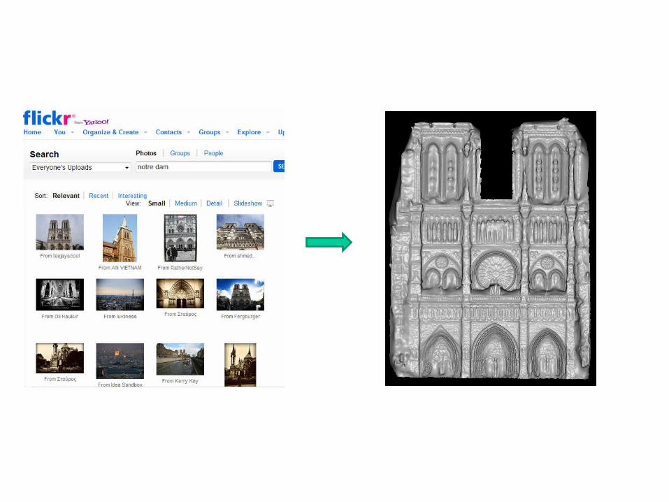
But there are some complications…Images taken in the wild – wide variety•Lots of photographers•Different cameras•Sampling rates •Occlusion•Different time of day, weather•Post processing

Trevi Fountain

Notre Dame

The problem statement•Design and analysis of an adaptive view selection process-given the massive number of images find a compatible subset of images

•Multi View Stereo (MVS)

- Reconstruct robust and accurate depth maps from image set

Previous Work (related to MVS)•Global View Selection- assume a relatively uniform viewpoint distribution and simply choose the k nearest images for each reference view.

•Local View Selection- use shiftable windows in time to adaptively choose frames to match

CPC datasets are more challenging Traditionally, multi-view stereo algorithms- far less appearance variation- somewhat regular distributions of viewpoints (e.g., photographs regularly spaced around an object, or video streams with spatiotemporal coherence)

CPC non-uniformly distributed in a 7D viewpoint (translation, rotation, focal length) space- represents an extreme case of unorganized image sets

Algorithm Overview•Calibrating Internet Photos

•View Selection

- Global View Selection

- Local View Selection

- Multi-View Stereo Reconstruction

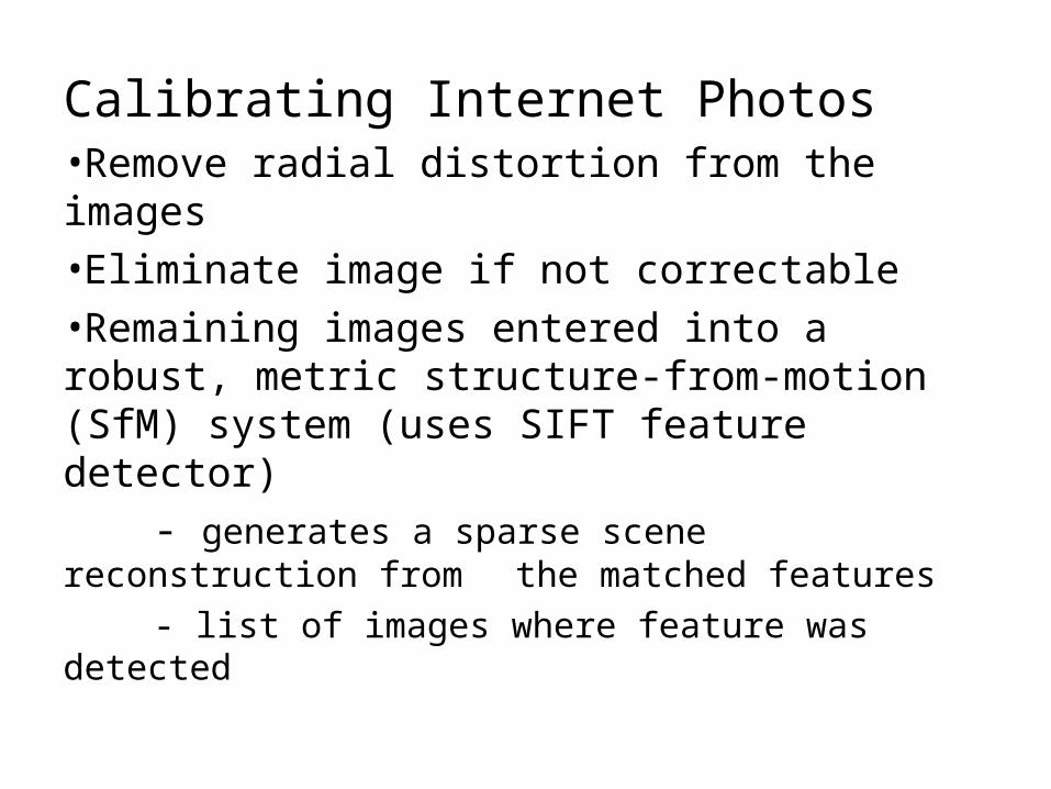
Calibrating Internet Photos•Remove radial distortion from the images

•Eliminate image if not correctable

•Remaining images entered into a robust, metric structure-from-motion (SfM) system (uses SIFT feature detector)

- generates a sparse scene reconstruction from the matched features

- list of images where feature was detected

• Remove Radiometric Distortions

- all input images into a linear radiometric space (sRGB color space)

View Selection - Global View Selection For each reference view R, global view selection seeks a set N of neighboring views that are good candidates for stereo matching in terms of scene content, appearance, and scale

SIFT selects features with similar appearance

•Shared Feature Points - problem of Collocation

•Scale Invariance - problem with stereo matching

Compute a global score gR for each view V within a candidate neighborhood N (which includes R)

FX - set of feature points observed in view XwN(f) – measures angular separationws(f) – measures similarity in scale

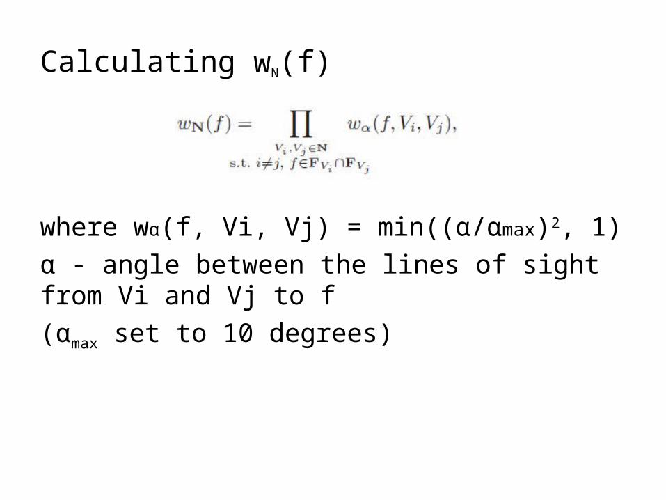
Calculating wN(f)

where wα(f, Vi, Vj) = min((α/αmax)2, 1) α - angle between the lines of sight from Vi and Vj to f(αmax set to 10 degrees)

Calculating wS(f)sV (f) - diameter of a sphere centered at f in V

Similarly sR(f) for R

the ratio r = sR(f)/sV (f)

- favors views with equal or higher resolution than the reference view

Add scores of all feature points for all views V and select top N

ΣV N∈ gR(v)

- greedy iterative approach

Rescaling Views-find the lowest resolution view Vmin, resample R-resample images of higher resolution

Multi-View Stereo ReconstructionTwo parts – Region-growing and Stereo Matching

Region-growing a successfully matched depth sample provides a good initial estimate for depth, normal, and matching confidence for the neighboring pixel locations in R- Has a priority queue containing candidate points-Initialized with SfM features in R along with features in V projected onto R-Run stereo matching and update q for each point

Stereo MatchingConsider n*n window centered on point in RGoal – To maximize photometric consistency of this patch to its projections into the neighboring views

Scene Geometry ModelPhotometric Model

Scene Geometry Model

-Window centered at pixel (s, t)

-oR is the center of projection of view R

-rR(s, t) is the normalized ray direction through the pixel

- Reference view corresponds to a point xR(s, t) at a distance h(s, t) along the viewing ray rR(s, t)

now, look at the neighbors

with i, j = −(n−1)/2 to (n−1)/2

- Determine the corresponding locations in a neighboring view k with sub-pixel accuracy using that view’s projection Pk(xR(s+i, t+j))

Photometric ModelSimple model for reflectance effects—a color scale factor ck for each patch projected into the k-th neighboring view

-Models Lambertian reflectance for constant illumination over planar surfaces-Fails for shadow boundaries, caustics, specular highlights, bumpy surfaces

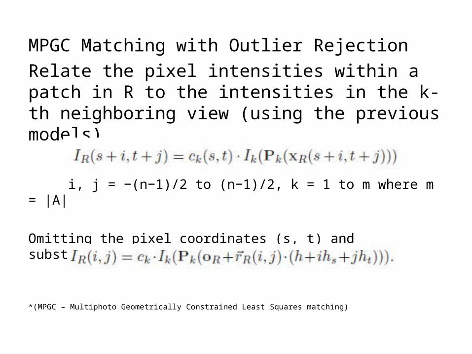
MPGC Matching with Outlier RejectionRelate the pixel intensities within a patch in R to the intensities in the k-th neighboring view (using the previous models)

i, j = −(n−1)/2 to (n−1)/2, k = 1 to m where m = |A|

Omitting the pixel coordinates (s, t) and substituting

*(MPGC – Multiphoto Geometrically Constrained Least Squares matching)

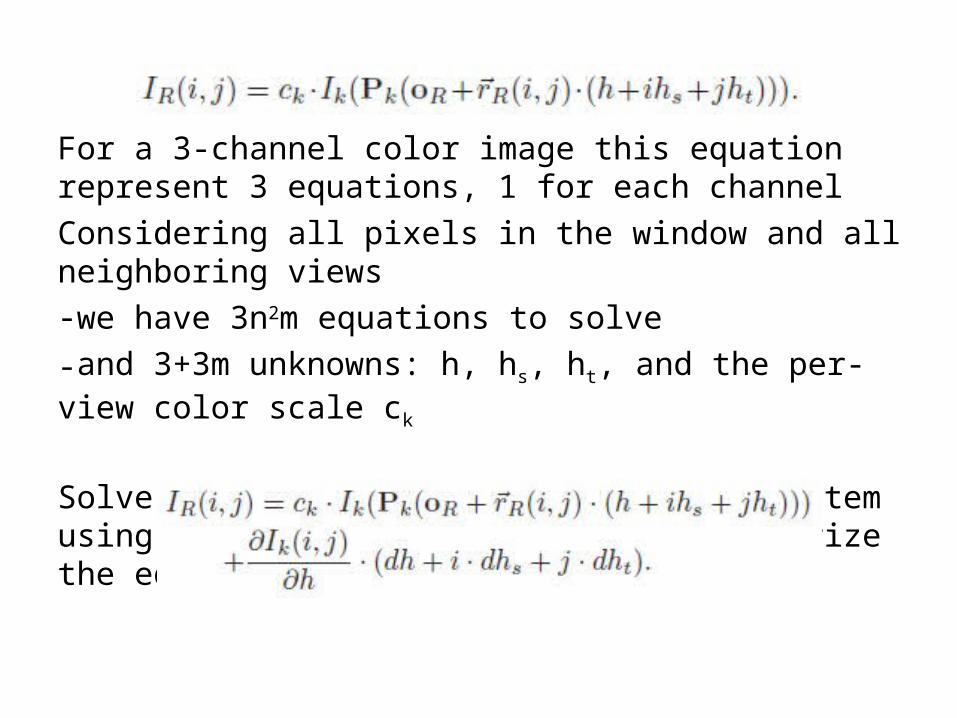
For a 3-channel color image this equation represent 3 equations, 1 for each channel

Considering all pixels in the window and all neighboring views

-we have 3n2m equations to solve

-and 3+3m unknowns: h, hs, ht, and the per-view color scale ck

Solve this over determined nonlinear system using the standard MPGC approach (linearize the equation)

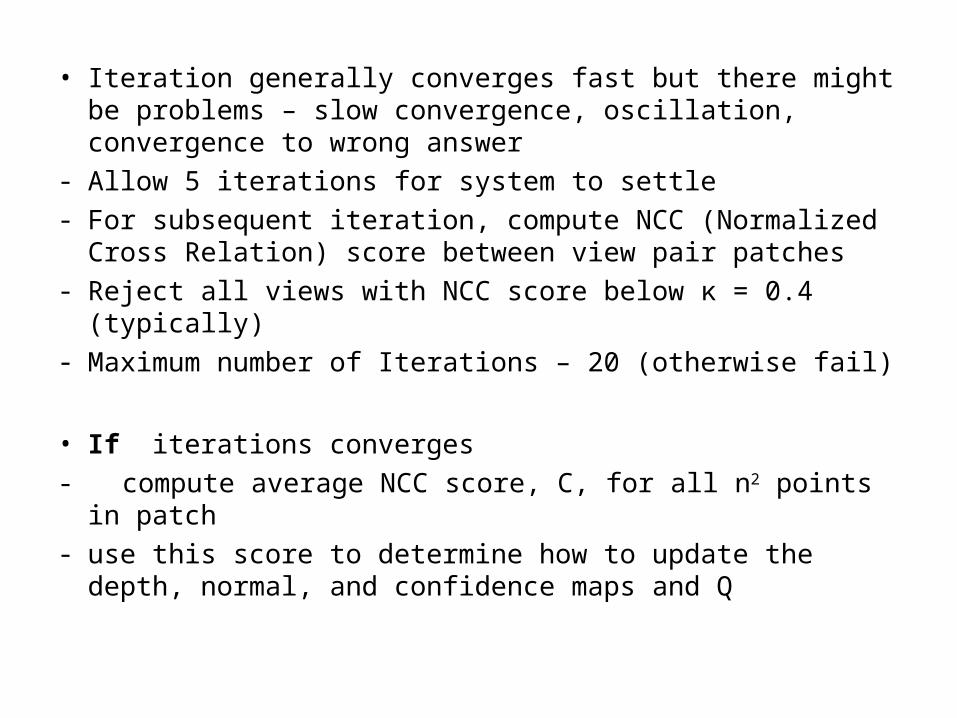
• Iteration generally converges fast but there might be problems – slow convergence, oscillation, convergence to wrong answer

- Allow 5 iterations for system to settle- For subsequent iteration, compute NCC (Normalized Cross

Relation) score between view pair patches - Reject all views with NCC score below κ = 0.4 (typically)- Maximum number of Iterations – 20 (otherwise fail)

• If iterations converges- compute average NCC score, C, for all n2 points in patch- use this score to determine how to update the depth, normal,

and confidence maps and Q

…continuing with Local View Selection•We now have a possible candidate V that can be added to A

Check for useful range of parallax - during Local View Selection we used α to avoid pictures with small triangulation angle - we now use a parameter γ (γmax = 10 degrees) to reduce weight of those images which are nearly co-planar (weighting system similar to previous case)

• If a view has a sufficiently high NCC score and satisfies parallax constraints, add to A

Repeat process, select from remaining non-rejected views, until either the set A reaches desired size or no non-rejected views remain.

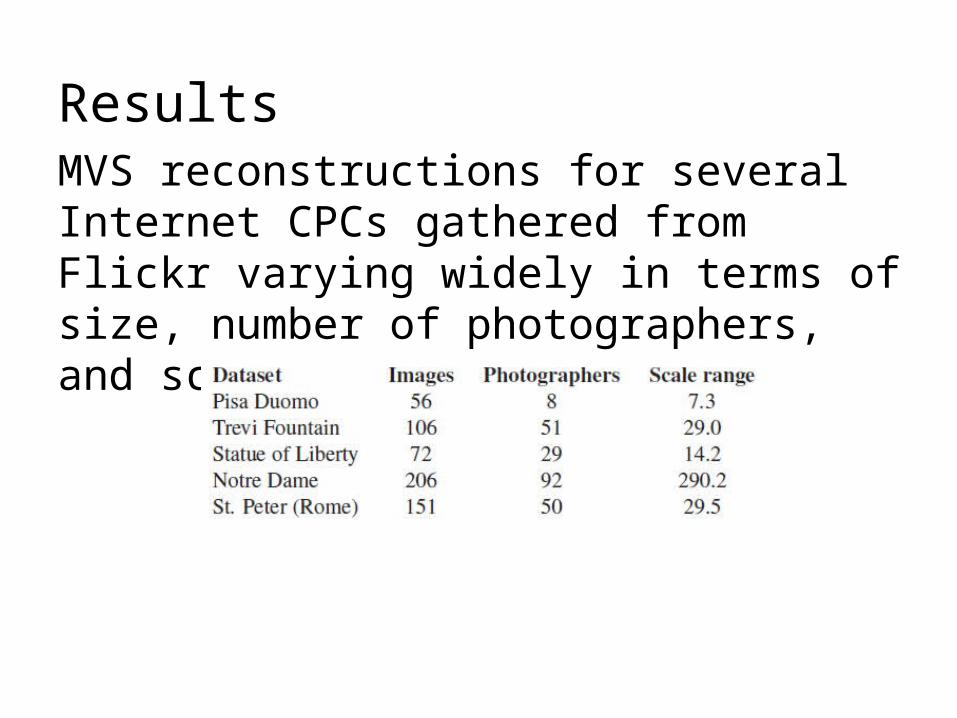
ResultsMVS reconstructions for several Internet CPCs gathered from Flickr varying widely in terms of size, number of photographers, and scale

Output

Reconstruction for Pisa Duomo

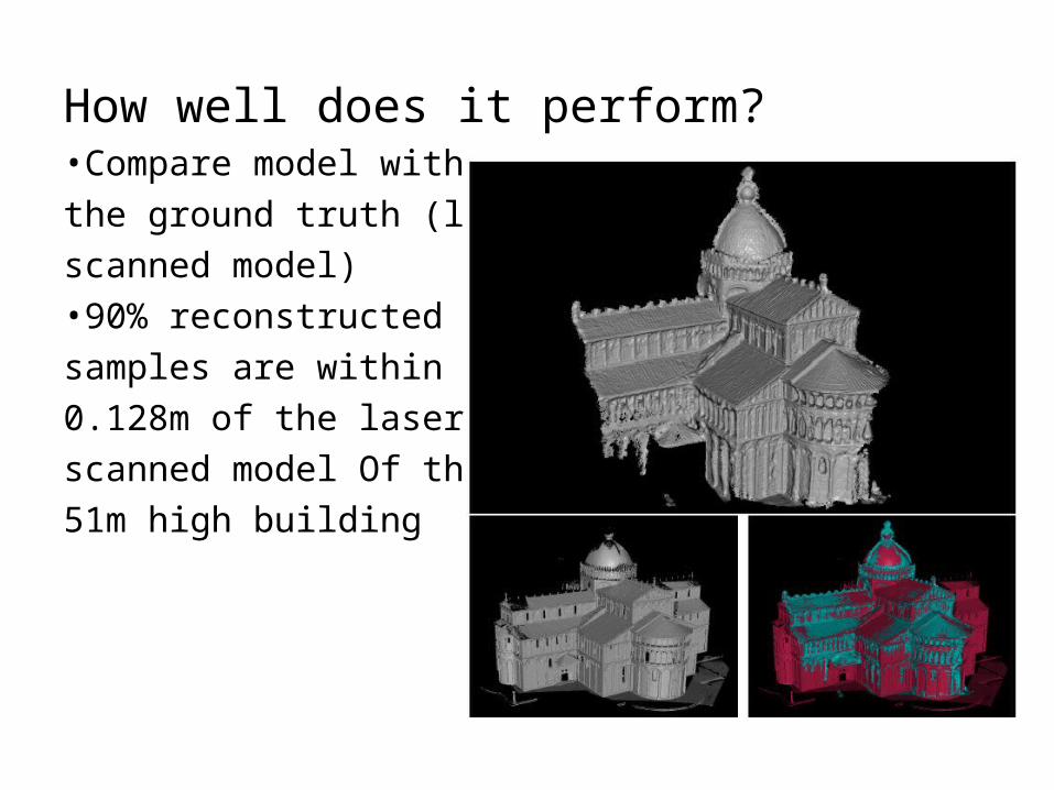
How well does it perform?•Compare model with

the ground truth (laser

scanned model)

•90% reconstructed

samples are within

0.128m of the laser

scanned model Of this

51m high building

Conclusion•Multi-view stereo algorithm capable of computing high quality reconstructions of a wide range of scenes from large, shared, multi-user photo collections available on the Internet•With the explosion of imagery available online, this capability opens up the exciting possibility of computing accurate geometric models of the world’s sites, cities, and landscapes

Reconstructing Building Interiors from Images

Yasutaka Furukawa, Brian Curless, Steven M. Seitz, Richard Szeliski

http://grail.cs.washington.edu/projects/interior/

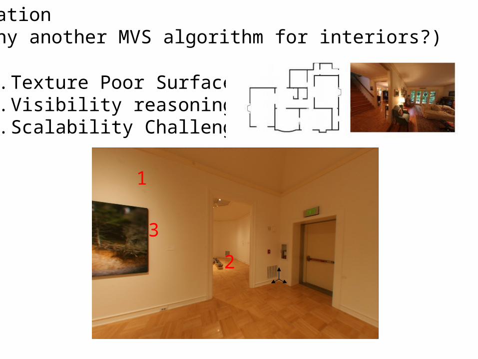
Motivation (or why another MVS algorithm for interiors?)

1. Texture Poor Surfaces2. Visibility reasoning3. Scalability Challenge

3

1

2

Incomplete 3D Reconstruction of the kitchen data set

3D Reconstruction Pipeline

1. 3D Location2. Surface Normal3. Set of Visible images Vi ={I1, I2, …..}

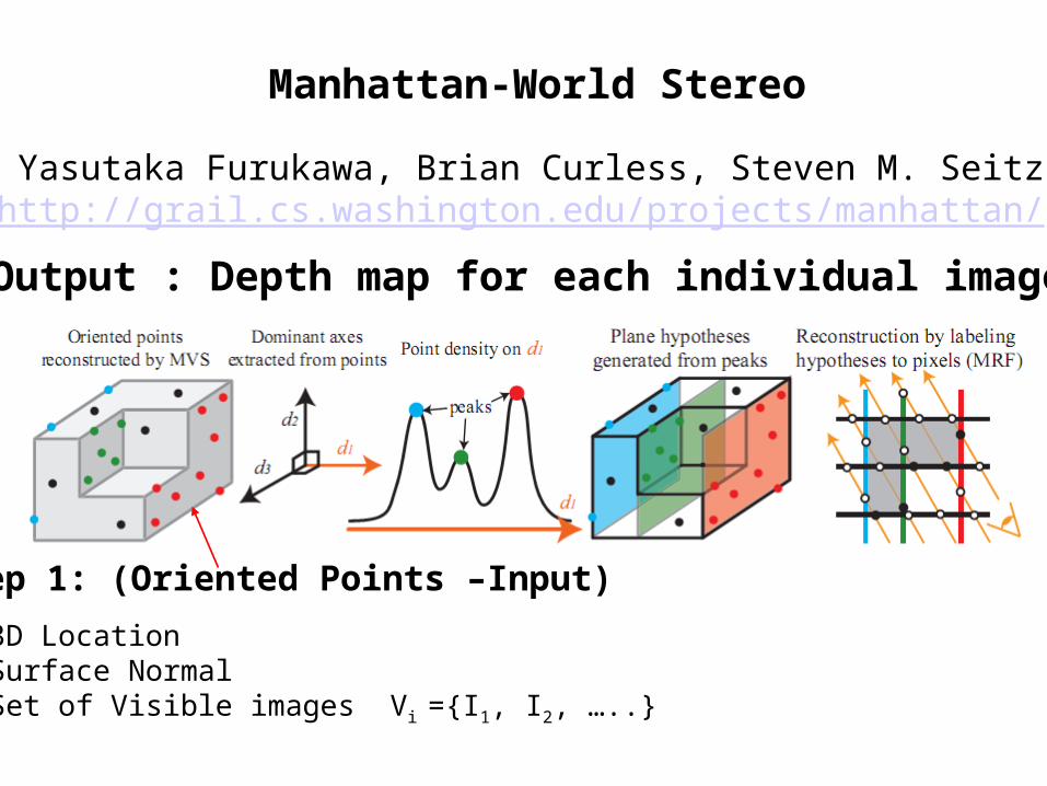
Manhattan-World Stereo

Yasutaka Furukawa, Brian Curless, Steven M. Seitzhttp://grail.cs.washington.edu/projects/manhattan/

• 3D Location• Surface Normal• Set of Visible images Vi ={I1, I2, …..}

Step 1: (Oriented Points –Input)

Output : Depth map for each individual image

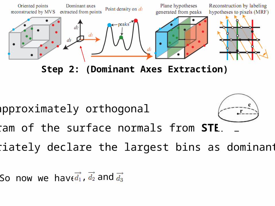
Step 2: (Dominant Axes Extraction)

•Only approximately orthogonal

•Histogram of the surface normals from STEP 1

•Appropriately declare the largest bins as dominant axes.

So now we have , and

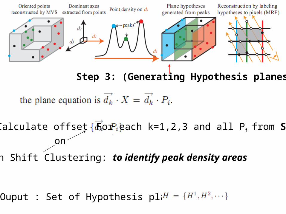
Step 3: (Generating Hypothesis planes)

Calculate offsets For each k=1,2,3 and all Pi from STEP 1

Mean Shift Clustering: to identify peak density areas

on

Ouput : Set of Hypothesis planes

Mean shift clustering

Data Set: X={x1, x2, …….. xn}

For each x in X

1. Calculate

where Is a Gaussian kernel

2. Shift x to m(x).

3. Repeat steps 1 to 3 until x converges to m(x)

D. Comaniciu and P. Meer.Mean shift: A robust approach toward feature space analysis.IEEE:PAMI, 24(5):603–619, May 2002.

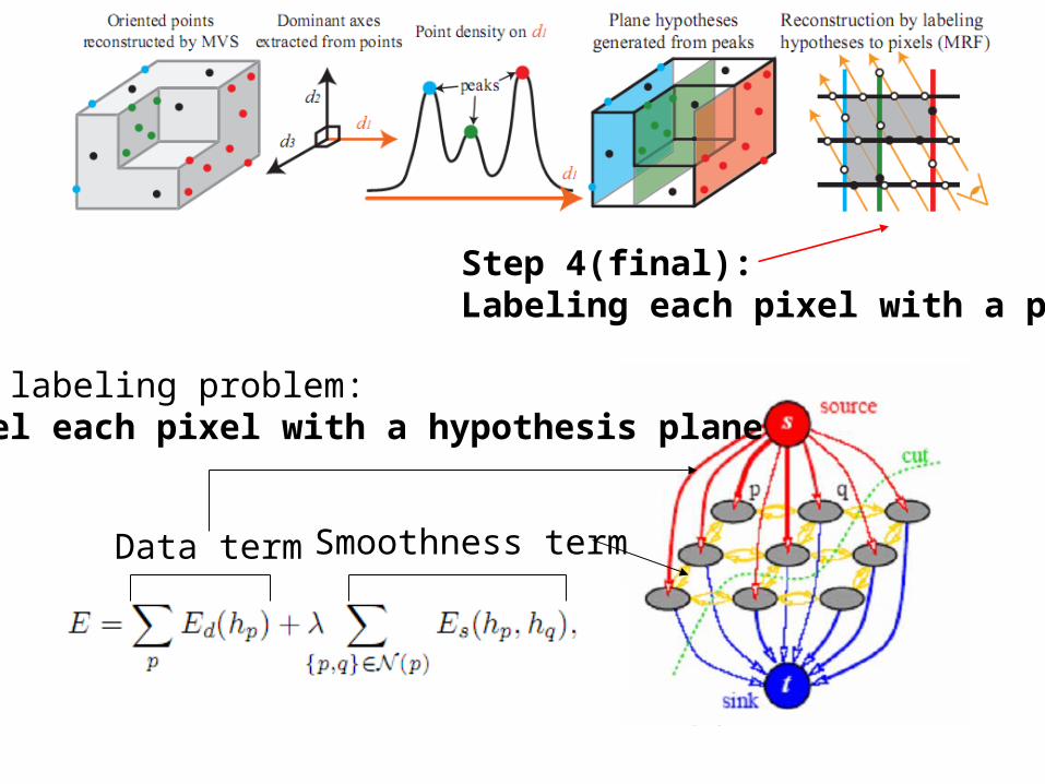
Step 4(final):Labeling each pixel with a plane

The labeling problem: Label each pixel with a hypothesis plane

Data term Smoothness term

Data term

Conflicts:

Smoothness term

We make use of priors (evidence) here : edges

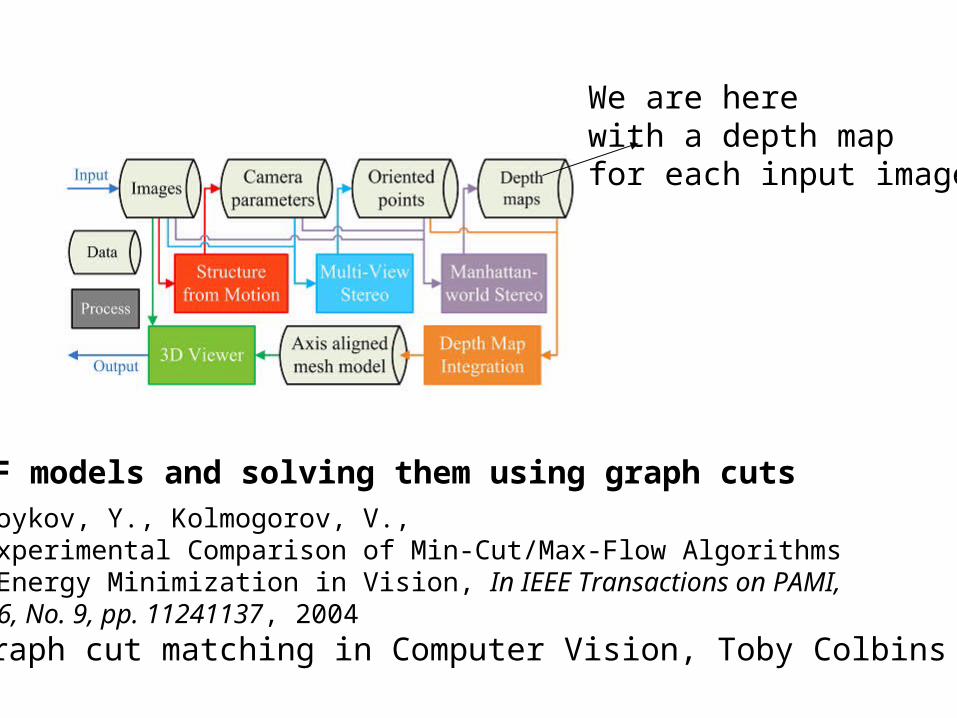
We are herewith a depth mapfor each input image

MRF models and solving them using graph cuts1. Boykov, Y., Kolmogorov, V., An Experimental Comparison of Min-Cut/Max-Flow Algorithmsfor Energy Minimization in Vision, In IEEE Transactions on PAMI,Vol. 26, No. 9, pp. 11241137, 2004

2.Graph cut matching in Computer Vision, Toby Colbins

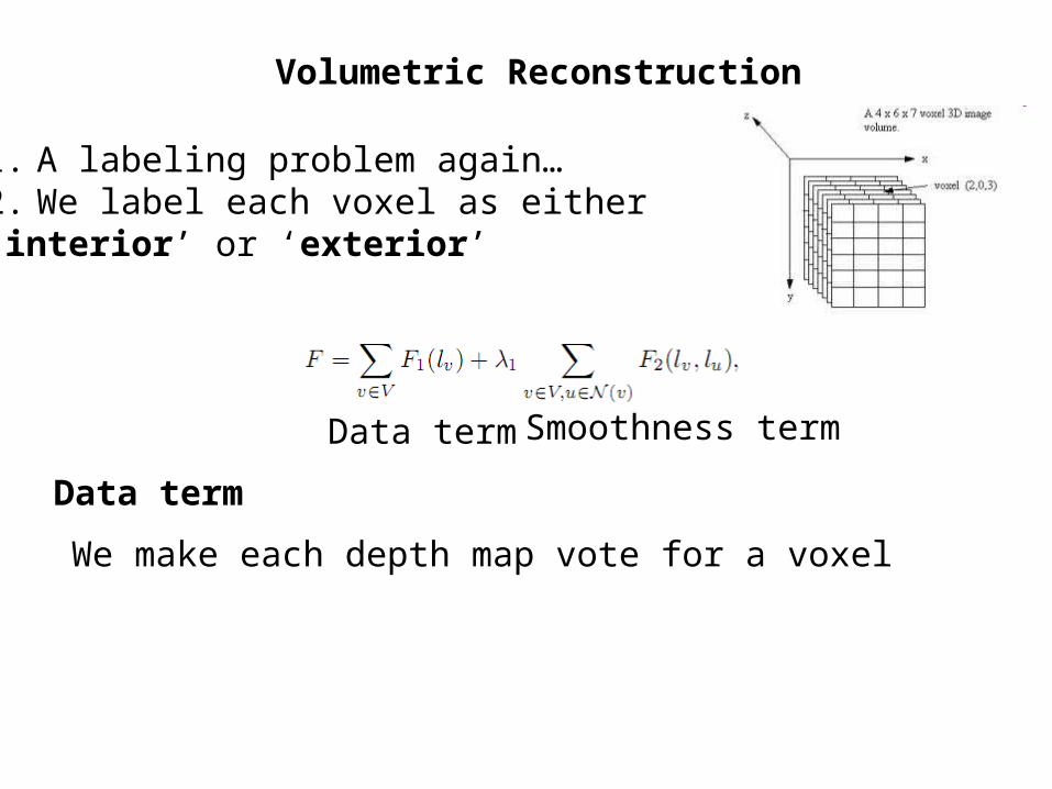
Volumetric Reconstruction

1. A labeling problem again…2. We label each voxel as either ‘interior’ or ‘exterior’

Data term Smoothness term

Data term

We make each depth map vote for a voxel

Notations: Pv

V

If v is behind pv, then it is labeled interior.

If v is in the front of pv, it is exterior.

1. We ask each depth map for a given voxel.

2. The depth map may vote a voxel as interior, exterior or empty(no visibility).

3. Majority wins.

Corner case:What if a depth map votesthe voxel as empty?

We take it as a vote forexterior.

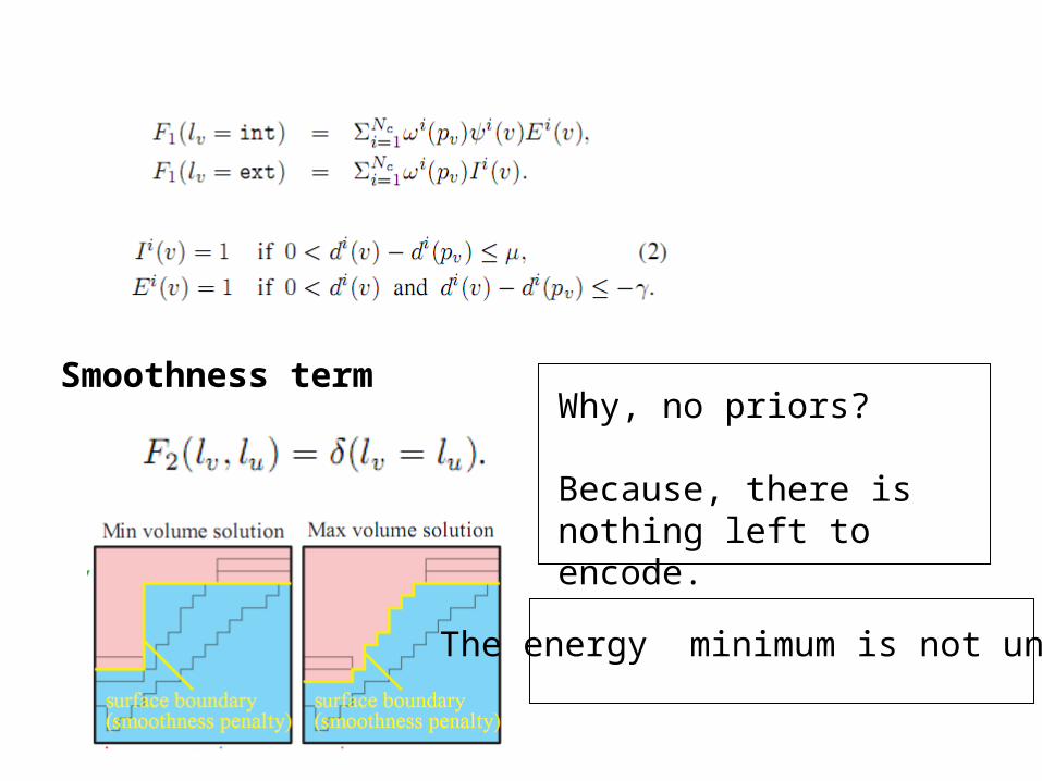
Smoothness termWhy, no priors?

Because, there is nothing left to encode.

The energy minimum is not unique

Now we have labeled each voxel as interior or exterior.

Delaunay triangulationDelaunay triangulationsmaximize the minimum angle of all the angles of the triangles in the triangulation; they tend to avoid skinny triangles.

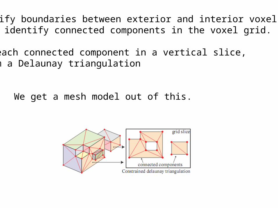
1. Identify boundaries between exterior and interior voxel regions.2. Hence identify connected components in the voxel grid.

3. For each connected component in a vertical slice, perform a Delaunay triangulation

We get a mesh model out of this.

A list of optimizations before we get the 3D model

1. Grid Pruning:

Remove a couple of grid slices.We want grid slices to pass through “grid pixels”.

2. Ground Plane determination:

The system has very little idea of the ground.

The bottom most horizontal slice with a lot of “grid pixels”

Or the bottom most slice with a count greater than the average.

3. Boundary filling

Building Rome in a DaySameer Agarwal, Noah Snavely, Ian Simon, Steven M. Seitz,

Richard Szeliski

http://grail.cs.washington.edu/rome/

City-scale 3D reconstruction•Search term “Rome” on flickr.com returns more than two million photographs•Construct a 3D Rome from unstructured photo collections

The Cluster•Images are available on a central store•Distributed to the cluster nodes on demand in chunks of fixed size

Overall System Design

Preprocessing and feature extraction•Down sample images•Convert to grayscale•Extract features using SIFT

Image Matching•Pairwise matching of images extremely expensive (Rome dataset – 100,000 images – 11.5 days)

•Use a multi-stage matching scheme. Each stage consists of a proposal and a verification step

Vocabulary Tree Proposals•Represent an image as a bag of words•obtain term frequency (TF) vector for image, and document frequency (DF) for image corpus•Per node TFIDF matrix – broadcast to cluster•Calculate TFIDF product (from own and cluster)•Top scoring k1+k2 images identified

Verification and detailed matching•Images distributed over cluster – problem •Experimented with 3 approaches (master node has all images to be verified)-optimize network transfers before any verification-overpartition image set into small set and send to node on demand-greedy bin packing •Verify image at node

Match Graph

•A graph on the set of images with edges connecting two images if matching features were found between them

•We want the fewest number of connected components in this graph

•Use the vocabulary tree for this

Track Generation•Combine all the pairwise matching information to generate consistent tracks across images.•Gather them at the master node and broadcast•Simultaneously, store the 2D coordinates and pixel color of •The feature points for using it in 3D rendering.•Refine the tracks

Geometric Estimation•Internet photo sets are redundant.•Incremental construction will be very slow.•Form a minimal skeletal set of photos such that connectivity is preserved.

Distributed Computing engine • Choices of file systems. Memory /speed tradeoffs• Whether multi platform (Unix /Windows)• Caching• Scheduling (map reduce)