Atmos. Chem. Phys., 18, 6939–6958, 2018https://doi.org/10.5194/acp-18-6939-2018© Author(s) 2018. This work is distributed underthe Creative Commons Attribution 4.0 License.

Multi-year assimilation of IASI and MLS ozone retrievals:variability of tropospheric ozone over the tropicsin response to ENSOHélène Peiro1, Emanuele Emili1, Daniel Cariolle1,2, Brice Barret3, and Eric Le Flochmoën3

1CECI, Université de Toulouse, Cerfacs, CNRS, Toulouse, France2Météo-France, Toulouse, France3Laboratoire d’Aérologie, Université de Toulouse, CNRS, UPS, Toulouse, France

Correspondence: Hélène Peiro (peiro@cerfacs.fr)

Received: 15 September 2017 – Discussion started: 15 November 2017Revised: 15 April 2018 – Accepted: 20 April 2018 – Published: 17 May 2018

Abstract. The Infrared Atmospheric Sounder Instru-ment (IASI) allows global coverage with very high spa-tial resolution and its measurements are promising for long-term ozone monitoring. In this study, Microwave LimbSounder (MLS) O3 profiles and IASI O3 partial columns(1013.25–345 hPa) are assimilated in a chemistry transportmodel to produce 6-hourly analyses of tropospheric ozonefor 6 years (2008–2013). We have compared and evaluatedthe IASI-MLS analysis and the MLS analysis to assess theadded value of IASI measurements.

The global chemical transport model MOCAGE (MOd-èle de Chimie Atmosphérique à Grande Echelle) has beenused with a linear ozone chemistry scheme and meteorologi-cal forcing fields from ERA-Interim (ECMWF global reanal-ysis) with a horizontal resolution of 2◦× 2◦ and 60 verticallevels. The MLS and IASI O3 retrievals have been assim-ilated with a 4-D variational algorithm to constrain strato-spheric and tropospheric ozone respectively. The ozone anal-yses are validated against ozone soundings and troposphericcolumn ozone (TCO) from the OMI-MLS residual method.In addition, an Ozone ENSO Index (OEI) is computed fromthe analysis to validate the TCO variability during the ENSOevents.

We show that the assimilation of IASI reproduces the vari-ability of tropospheric ozone well during the period understudy. The variability deduced from the IASI-MLS analysisand the OMI-MLS measurements are similar for the periodof study. The IASI-MLS analysis can reproduce the extremeoscillation of tropospheric ozone caused by ENSO eventsover the tropical Pacific Ocean, although a correction is re-

quired to reduce a constant bias present in the IASI-MLSanalysis.

1 Introduction

Tropospheric ozone (O3) is the third most important green-house gas (Houghton et al., 2001). It influences the atmo-spheric radiative forcing as one of the main absorbers ofinfrared and ultraviolet radiation (Wang et al., 1980; Laciset al., 1990). It also has a strong effect on human healthand vegetation. High levels of O3 concentrations increasepulmonary and chronic respiratory diseases, increasing hu-man premature mortality (Guilbert, 2003; Bell et al., 2004;Ebi and McGregor, 2008). High concentrations of O3 re-duce photosynthesis and other important physiological func-tions of vegetation (Yendrek et al., 2015). Due to its rel-atively long lifetime (∼ 2 weeks in the troposphere), theglobal variability of tropospheric ozone is the combination ofthe complex interactions between anthropogenic emissions,chemical production and destruction, long-range transport,and stratosphere–troposphere exchanges. A global increasein tropospheric ozone has been documented during the last30 years (Cooper et al., 2014), the cause of which is not yetwell understood (Fowler et al., 2008). To determine the originof this trend, it is important to evaluate the relative contribu-tions between natural variability and anthropogenic forcing.

Among the natural forcings, the El Niño Southern Oscil-lation (ENSO) is an atmospheric phenomenon with a large-

Published by Copernicus Publications on behalf of the European Geosciences Union.

6940 H. Peiro et al.: Tropospheric Ozone in response to ENSO

scale circulation pattern that influences the O3 distribution(Chandra et al., 1998; Zeng and Pyle, 2005) with a peri-odicity of about 2–7 years. ENSO refers to two events inthe tropical Eastern Pacific: El Niño (anomalously warmocean temperatures) and La Niña (anomalously cold oceantemperatures). ENSO is the dominant source of the tropicalPacific variability for the atmosphere and the ocean (Tren-berth, 1997; Philander, 1989). During ENSO, changes insea-surface temperatures (SSTs) in the Pacific Ocean have alarge influence on the normal atmospheric circulation, dis-placing the location of convection and its intensity (Quanet al., 2004). These changes in circulation impact the tem-perature and moisture fields across the tropical Pacific, influ-encing the chemical composition of the troposphere (Ziemkeand Chandra, 2003; Randel and Thompson, 2011, Fig. 1).

Convection during ENSO affects tropical tropospheric O3in two ways. First, convection impacts the vertical mixingof O3 itself. Convection lifts lower tropospheric air masseswith a low ozone concentration, where O3 lifetime is shorter,to upper troposphere where O3 lifetime is longer (Dohertyet al., 2005). Overall increased convection leads to a decreasein the tropospheric ozone column (Fig. 1a). Second, convec-tion affects vertical mixing and vertical distribution of O3precursors (Stevenson et al., 2005). El Niño events coincidewith dry conditions generating large-scale biomass burningin Indonesia (Chandra et al., 2002). During El Niño, TCOover Indonesia is higher than average. A remarkable changein the tropospheric O3 concentration due to El Niño occurredin the western part of Pacific during 1997–1998, with an in-crease in the TCO of +20 to +25 DU (Chandra et al., 2002).Atmospheric particulates and O3 precursors increase in In-donesia (Fig. 1b). During La Niña events, dry conditions arelocated in South America, causing an increase of TCO in theeastern Pacific Ocean (Fig. 1c).

Previous studies have characterized the variations of thetropical tropospheric O3 linked to ENSO (Ziemke et al.,2015). To characterize the ENSO amplitude several ENSOindices have been proposed based on ENSO footprints onthe pressure field or the outgoing longwave radiation (Ar-danuy and Lee Kyle, 1985; Trenberth, 1997). Ziemke et al.(2010) developed such an index for Ozone, the Ozone ENSOIndex (OEI), to better characterize the effect of the oscilla-tion on the O3 distribution and as a diagnostic tool for tropo-spheric chemistry models.

A detailed analysis of the effects of convection on tropo-spheric O3 has been prevented so far by the paucity of ob-servations (Solomon et al., 2005; Lee et al., 2010). The re-stricted number of ozonesonde observations limits analysisof the links between O3 and ENSO (Thompson et al., 2003).Satellite observations can give more information on the O3variability, and their global coverage gives better insight intothe processes involved in ENSO (Ziemke et al., 2010). Toderive tropospheric O3 several studies have combined ozonemeasurements from the Ozone Monitoring Instrument (OMI)that measures the total ozone columns, and the Microwave

Figure 1. Schematic of the Walker circulation over the Pacificocean. (a) During normal conditions: trade winds induce subsidencealong South America with intrusion of O3-rich air. The TCO is el-evated. In addition, along Indonesia, warmer waters generate con-vergence that results in low O3 concentrations. The TCO is weak-ened (b) during El Niño events: easterly trade winds are weakened.Therefore, convergence areas are located near the coast of SouthAmerica while subsidence zones are located in the Indonesia. LowTCO is located over the Pacific ocean while high TCO is locatedover Indonesia, and (c) during La Niña events: during exceptionallystrong trade winds the convergence over the Indonesia is stronger.The TCO has the lowest value. Subsidence over South Americabrings air masses with high O3 concentration, resulting in higherTCO than average values.

Atmos. Chem. Phys., 18, 6939–6958, 2018 www.atmos-chem-phys.net/18/6939/2018/

H. Peiro et al.: Tropospheric Ozone in response to ENSO 6941

Limb Sounder (MLS) that provides vertical ozone profiles inthe upper troposphere and stratosphere. Ziemke et al. (2006)subtracted the stratospheric column O3 (of MLS) from thetotal column O3 (of OMI) to obtain the tropospheric columnO3 (named hereafter OMI-MLS). They show a large impactof ENSO on tropospheric O3 in the tropics by analyzing theOMI-MLS data (Ziemke et al., 2015). The O3 sensitivity toENSO was also studied with the tropospheric emission spec-trometer (TES) observations (Neu et al., 2014). They stud-ied, during El Niño, the long-range transport of Asian pol-lution due to the Northern Hemisphere subtropical jet. MLSand TES data were also compared to a chemistry–climatemodel to study how ENSO can influence the O3 distribu-tion (Oman et al., 2013). These studies demonstrate that thelink between O3 and ENSO becomes a key element of thechemistry–climate interactions.

The combination of OMI and MLS measurements al-lows insights into the links between tropospheric O3 andENSO, but has limitations because the tropospheric partialO3 columns are obtained as a difference between two largequantities, the total column and the stratospheric column.Hence, possible bias and errors in MLS and OMI data can beamplified when the partial tropospheric column is calculated.The objective of the present study is to obtain direct evalua-tions of tropospheric ozone using assimilation of ozone pro-files from MLS and from IASI.

The IASI instrument, launched onboard MetOp-A in 2006,was designed for numerical weather predictions and atmo-spheric composition observations (Clerbaux et al., 2009).IASI allows a daily global coverage at very high spatial res-olution (12 km for nadir observations). Because of its spatialcoverage, the day and night retrieval coverage, IASI providesan important added value with respect to other satellites likeTES or OMI (Herbin et al., 2009; Pittman et al., 2009; Oet-jen et al., 2016). The IASI mission is meant to last for sev-eral decades (MetOp) whereas the instruments OMI, MLSand TES are scientific missions with limited lifespan. Tro-pospheric O3 from IASI has been already studied and val-idated. The IASI ozone data were found to be particularlywell suited to the study of O3 variations in the upper tropo-sphere (Dufour et al., 2012; Tocquer et al., 2015; Barret et al.,2016). Since we already have about 10 years of data, theIASI mission provides a valuable dataset to study the O3 vari-ability and trends (Toihir et al., 2015; Wespes et al., 2016),both in the troposphere and the stratosphere (Wespes et al.,2009, 2012; Dufour et al., 2010; Barret et al., 2011; Scannellet al., 2012; Safieddine et al., 2013). More recently, the tro-pospheric O3 variability due to ENSO has been studied using8 years (January 2008 to March 2016) of IASI measurements(Wespes et al., 2017). They have shown that IASI retrievalscan capture the variability of tropospheric ozone related tothe large-scale dynamical modes of ENSO.

By assimilating IASI data within the MOCAGE model(Teyssèdre et al., 2007), we expect to obtain O3 distribu-tions consistent with OMI-MLS observations and to have

additional information on the vertical O3 distributions inthe troposphere. We use the MOCAGE chemistry transportmodel (CTM) to assimilate tropospheric ozone profiles fromIASI and stratospheric profiles from MLS with a 4D-Var (4-dimensional-variational) algorithm. The joint assimilation ofIASI and MLS data was already found to improve modeledO3 in the UTLS (Barré et al., 2013; Emili et al., 2014). Sincethe information in IASI retrievals is strongly weighted in thetroposphere, the assimilation of MLS allows the introductionof complementary information in the case of stratosphere–troposphere exchanges (Barré et al., 2012), which intensifyover the eastern Pacific Ocean during the La Niña phase ofthe ENSO. We will evaluate in this study the relative impor-tance of assimilating MLS and IASI in the context of the O3variability related to ENSO. To compute ozone tendenciesMOCAGE uses the latest version of the linear ozone chem-istry parametrization of Cariolle and Teyssedre (CARIOLLEScheme, 2007).

The influence of ENSO on tropical tropospheric O3 hasbeen simulated by CTMs or by global chemistry–climatemodels (Sudo and Takahashi, 2001a; Zeng and Pyle, 2005;Doherty et al., 2006; Oman et al., 2011). Fewer studies useddata assimilation to study the distribution and interannualvariability of tropospheric ozone in the Pacific (Liu et al.,2017; Olsen et al., 2016). Data assimilation allows time se-ries of chemical fields that integrate all available informationfrom measurements and models to be obtained. This can beparticularly useful when tropospheric retrievals from satel-lite measurements become very sparse, due for instance tothe occurrence of convective clouds in the tropical region.Furthermore, the assimilation of IASI data for a long timeperiod has not yet been considered. The 6-year reanalysis(2008–2013) of tropospheric O3 that we have computed inthe present study is ideal for studying the ozone variability inthe tropics from short-term to interannual timescales.

The format of this paper is as follows. In Sect. 2 we de-scribe the observations used for assimilation and model val-idation, as well as the settings used by the MOCAGE modeland the assimilation suite. In Sect. 3 we discuss the resultsobtained assimilating IASI and MLS data, with an empha-sis on the impact of ENSO on tropospheric O3. We derivean Ozone ENSO Index and compare its evolution to previousstudies. The final section summarizes the results.

2 Methodology

2.1 Assimilated observations

2.1.1 IASI and MetOp-A measurements

The IASI is one of the instruments onboard the polar-orbitingsatellite MetOp-A (Meteorological Operational), which isoperated by the European organization for the exploitationof Meteorological Satellites (EUMETSAT). The MetOp-A

www.atmos-chem-phys.net/18/6939/2018/ Atmos. Chem. Phys., 18, 6939–6958, 2018

6942 H. Peiro et al.: Tropospheric Ozone in response to ENSO

satellite was launched on 19 October 2006 and has alreadyprovided data for about 10 years. Due to its inclination to theequatorial plane and its altitude (817 km), MetOp-A crossesthe equatorial plane at 09:30 and 21:30 LT (the equatorialplane at 9:30 and 21:30 local solar time when crossing theEquator).

IASI is a nadir-viewing Fourier Transform Spectrometer.The detectors sense in the thermal infrared spectral rangebetween 645 and 2760 cm−1 (15.5 to 3.62 µm). IASI pro-vides spectra with a high radiometric quality at a resolu-tion of 0.5 cm−1 (after apodization). IASI measurements aretaken along- and across-track over a swath width of 2200 kmwith an horizontal resolution of 12 km. Therefore, IASI pro-vides global coverage twice a day. The high spectral reso-lution of IASI allows the retrieval of vertical profiles of anumber of gases affecting the climate system and the atmo-spheric pollution (Clerbaux et al., 2009; Coheur et al., 2009).Previous studies have used vertical information from IASILevel 2 products to study O3 in the troposphere, in the up-per troposphere–lower stratosphere (UTLS) and in the strato-sphere (Dufour et al., 2010; Barret et al., 2011, 2016; Wespeset al., 2012; Tocquer et al., 2015).

A radiative transfer code and retrieval software are usedto retrieve O3 profiles from IASI radiances. We use O3 re-trievals performed with the Software for Fast Retrieval ofIASI Data (Barret et al., 2011) developed at Laboratoireof Aerology. The SOFRID (SOftware for a Fast Retrievalof IASI Data) is based on the RTTOV (Radiative Transferfor TOVS, Saunders et al., 1999a, b) fast radiative transfermodel coupled to the 1D-Var algorithm developed at UKMO(United Kingdom Met Office, Pavelin et al., 2008). SOFRIDretrieves the O3 profiles on 43 levels from 1013.25 to 0.1 hPausing a single a priori profile and covariance matrix basedon 1 year of in situ observations (see Barret et al., 2011 fordetails). Validation of 6 months of tropospheric O3 columnsfrom IASI-SOFRID against ozonesondes and airborne datahave shown biases of about 5 % and relative standard devi-ation (RSD) of about 15 % in the tropics. In their validationstudy of three IASI O3 products over 1 year, Dufour et al.(2012) also found biases of 3.8 and RSD of 9.5 % for IASI-SOFRID tropospheric O3 relative to ozonesonde data in thetropics. In this study, partial O3 columns between 1013.25and 345 hPa has been computed from the IASI-SOFRID pro-file prior to the assimilation.

2.1.2 MLS measurements

The MLS instrument flies onboard the Aura satellite in a po-lar orbit with a continuous record that begins in July 2004.The Aura spacecraft has an equatorial crossing time of 13:45(local solar equatorial crossing time of 13:45) (ascendingnode) with approximately 15 orbits per day on average. TheMLS measures thermal emissions at the atmospheric limband provides vertical profiles of several atmospheric con-stituents (Waters et al., 2006). MLS allows the retrieval of

about 3500 profiles per day with a nearly global spatial cov-erage between 82◦ S and 82◦ N. Each profile is spaced byabout 165 km along the orbit track. The recommended usefulpressure range (Livesey et al., 2011) for the MLS measure-ments of the versions v3 and v4 is from 261 to 0.02 hPa, witha vertical resolution between 2.5 and 6 km, depending on al-titude.

For this study we used version 4.2 of the MLS ozone prod-uct (Schwartz et al., 2015). Notable improvements of thev4.2, compared to the earlier versions v3.3 and v3.4, showa reduction in the severity and frequency of cloud impactson ozone determination. For more information, users of MLSAura L2 v4.2 should refer to the EOS MLS Level 2 Version 4Quality Document by Livesey et al. (2016). MLS ozone pro-files show good quality in the UTLS, with a precision ofabout 5 %. Biases for MLS ozone profiles are about 2 % inthe stratosphere but they increase in the upper troposphereand can be as high as 20 % at the 215 hPa level (Froidevauxet al., 2008). To avoid the introduction of biases at this levelin our analyses we have taken the MLS ozone data only be-tween 12.12 and 177.83 hPa.

2.2 Validation measurements

2.2.1 The OMI-MLS residual method and the OzoneENSO Index

The OMI instrument, is one among a total of four instru-ments onboard the Aura satellite. It is a nadir-viewing imag-ing spectrometer that measures the solar radiation reflectedby Earth’s atmosphere and surface (Levelt et al., 2006). Itmakes spectral measurements in the ultraviolet (270–314 and306–380 nm) and visible 350–500 nm wavelength regions at0.5 nm resolution. OMI provides measurements with a dailyglobal coverage and a very high horizontal spatial resolutionof 13 km× 24 km at nadir (Dobber et al., 2006). Retrieval er-rors of the OMI data vary from 6 to 35 % in the troposphere(Liu et al., 2010). Total column ozone from OMI have beenderived using the TOMS version 8 algorithm (Ziemke et al.,2006).

To derive TCO with the OMI-MLS residual method,Ziemke et al. (2006) subtracted the stratospheric ozonecolumns retrieved with MLS from the OMI total column.They selected OMI pixels with near clear-sky conditions (ra-diative cloud fraction < 30 %). Stratospheric MLS data werespatially interpolated each day on a coarser regular grid. Thetropopause height used for the TCO cutoff between OMI andMLS comes from the National Centers for EnvironmentalPrediction (NCEP) using the 2 K km−1 lapse rate tropopausedefinition (Craig, 1965) of the World Meteorological Orga-nization (WMO). We used OMI-MLS data from the NASAGODDARD website for tropospheric ozone (http://acd-ext.gsfc.nasa.gov/Data_services/). All available daily data havebeen averaged to compute monthly means with a latitude–longitude resolution of 1◦× 1.25◦.

Atmos. Chem. Phys., 18, 6939–6958, 2018 www.atmos-chem-phys.net/18/6939/2018/

H. Peiro et al.: Tropospheric Ozone in response to ENSO 6943

There is no single universal ENSO index reproducingoceanic and atmospheric physical conditions over the tropi-cal Pacific (Trenberth, 1997). Many ENSO indices have beendeveloped using for instance SST and precipitation (Tren-berth, 1997; Curtis and Adler, 2000). The commonly usedNOAA Niño 3.4 index is derived from SST anomalies. Basedon 30 years of satellite measurements to investigate ENSO’simpact on tropical TCO, Ziemke et al. (2010) produced amonthly OEI. Stratospheric column ozone in the tropical Pa-cific has very small longitudinal variations of only a fewDobson units. This has been shown in the previous stud-ies from SAGE, UARS HALOE, UARS MLS and AURAMLS stratospheric O3 satellite measurements (Ziemke et al.,1998, 2010). Because of this characteristic, the zonal vari-ation of the TCO in the tropical Pacific is essentially iden-tical to the east–west variation of total column ozone. ThusTCO alone can be used to derive the OEI. The OEI is ob-tained by subtracting the TCO in the region named PacificOcean Center (POC, 15◦ S–15◦ N, 110–180◦W) from theTCO in the region Indonesia with Indian Ocean (IIO, 15◦ S–15◦ N, 70–140◦ E) each month. To compute the TCO, thealtitude of the tropopause must be known. Ziemke et al.(2010) used tropopause heights derived from the NCEP data.The tropopause is defined as the lowest level, with respectto altitude, at which the temperature lapse rate decreases to2 ◦C km−1 or less and does not exceed 2 K km−1 for 2 kmabove. We adopted this tropopause computation to derive theOEI from our analyses. Tropopause pressures, used to com-pute the Ozone Index with the assimilation of both IASI-MLS and MLS data only, are comprised between 80 hPa atlow latitudes and 500 hPa at high latitudes.

2.2.2 Ozonesondes

Ozonesondes are launched in many locations over the worldon a weekly basis, measuring vertical profiles of O3 concen-tration with a high vertical resolution of 150–200 m, fromthe ground to approximately 10 hPa. Data are collected bythe World Ozone and Ultraviolet Radiation Data Center(WOUDC, http://www.woudc.org). During the 6 years con-sidered in this study (2008 to 2013), only 270 ozone sound-ings are available for the Pacific area between 15◦ S–15◦ Nand 70◦ E–110◦W (Fig. 2). We divide this area into two re-gions: IIO and POC, which are represented by the two bluerectangles in Fig. 2.

WOUDC ozonesonde measurements used for the valida-tion are considered as a reference. Despite their sparse geo-graphical distribution, several studies have used the WOUDCdatabase to validate global models and satellite retrievals(Geer et al., 2006; Massart et al., 2009; Dufour et al., 2012).

Figure 2. Map of WOUDC ozonesonde localization between 15◦ Sand 15◦ N. The red circles mark ozonesonde stations between 70◦ Eand 110◦W. Green squares are ozonesonde stations elsewhere in thetropical band used hereafter. The two blue squares define the IIOregion (15◦ S–15◦ N and 70–140◦ E) and the POC region (15◦ S–15◦ N and 180–110◦W) referred to in this study.

2.3 Analyses

2.3.1 Chemical transport model

MOCAGE is a three-dimensional CTM based on a semi-Lagrangian advection scheme (Williamson and Rasch, 1989)developed for both tropospheric and stratospheric applica-tions. Multiple nested domains with different horizontal res-olutions can be used within MOCAGE, as well as chemi-cal and physical parameterizations of increasing complex-ity. The different configurations of MOCAGE have beenvalidated against in situ, satellite and ground-based mea-surements in several studies (Josse et al., 2004; Teyssèdreet al., 2007; Bousserez et al., 2007; Honoré et al., 2008; Sicet al., 2015). For this study, a global horizontal resolution of2◦× 2◦ has been used with 60 sigma hybrid vertical levelsfrom the surface up to 0.1 hPa. The vertical resolution goesfrom about 40 m in the boundary layer, to about 500 m in thefree troposphere and to approximately 800 m in the upper tro-posphere and lower stratosphere. The model uses winds, tem-perature and ground pressure from the European Center forMedium-Range Weather Forecasts (ECMWF) ERA-Interimreanalysis (Berrisford et al., 2011).

For the chemical scheme we use the simplified ozonechemistry scheme developed by Cariolle and Teyssedre(2007), based on the linearization of the destruction and pro-duction rates of ozone. Emili et al. (2014) have shown thatwith this simplified chemical scheme it is possible to ob-tain O3 analyses from IASI data of comparable quality tothose obtained using more complex chemical schemes. Theuse of this simplified scheme reduces numerical costs, whichis highly beneficial for the production of long chemical re-analyses such as the ones discussed in this study. Since thelinearized chemistry scheme does not have any longitudi-nal variation, the longitudinal ozone variability that is repro-duced by the model (e.g., in correspondence of the Walker

www.atmos-chem-phys.net/18/6939/2018/ Atmos. Chem. Phys., 18, 6939–6958, 2018

6944 H. Peiro et al.: Tropospheric Ozone in response to ENSO

circulation, see Sect. 3.2.1) results only from the ozone trans-port.

2.3.2 Assimilation algorithm

The chemical data assimilation system for MOCAGE is de-veloped at CERFACS and has already been used for sev-eral applications at both regional and global scales (El Am-raoui et al., 2010; Sic et al., 2016). The MOCAGE assim-ilation system was part of the first international exercise ofsatellite ozone assimilation (Geer et al., 2006) and it cur-rently provides operational air quality analyses for the eu-ropean project CAMS (Marécal et al., 2015). The assimila-tion configuration used for this study is based on the 4D-Var algorithm in a “perfect model” framework. Compared tothe 3D-Var algorithm, the 4D-Var allows a better exploita-tion of satellite observations with large spatial and temporalfingerprint (Massart et al., 2010). The cost function is mini-mized using the limited-memory BFGS (Broyden–Fletcher–Goldfarb–Shanno) method (Liu and Nocedal, 1989) and thethree-dimensional background error covariance matrix (B) ismodeled through a diffusion equation (Weaver and Courtier,2001).

The IASI partial O3 columns (1000–345 hPa) and MLSprofiles have been assimilated in the troposphere and in thestratosphere respectively to constrain the ozone concentra-tion along the full atmospheric column. For this study, thechoice of the assimilated column top (345 hPa) has beentaken based on SOFRID averaging kernels found over thetropics (Barret et al., 2011). The objective was to minimizethe extent of the atmospheric layer where both MLS and IASIcan have a direct impact. This avoids to some extent the needto quantify and account for possible biases between the twoinstruments. Before the assimilation, IASI data have been av-eraged to obtain 2◦ by 2◦ pixels to match the model resolu-tion. The smoothing equation based on the averaging kernels(AKs) and on the a priori profile in the troposphere has beenapplied to the profiles from the model to account for the lim-ited sensitivity of IASI retrievals in the troposphere (see Bar-ret et al., 2016). The description of the linear retrieval equa-tion can be found in Barret et al. (2011). Emili et al. (2014)found global biases of 10 % in the troposphere-assimilatingIASI-SOFRID product in MOCAGE. When they removed10 % of the values in the IASI observations, the biases inthe analyses were significantly reduced. The same correctionhas been applied in this study.

Most of the parameters of the assimilation algorithm usedto compute the reanalyses in this study are based on the studyof Emili et al. (2014). The validation of a short reanaly-sis of 2 months against ozonesondes (not shown) has beenused to further optimize some of these parameters. The back-ground and observation errors are defined as follows. Emiliet al. (2014) have assimilated IASI and MLS data globallywith a background error standard deviation equal to 30 %of the modeled ozone profile in the troposphere and 5 % in

the stratosphere. Based on local validation in the tropics, wefound slightly superior results using an error standard devia-tion of 15 instead of 30 % in the troposphere. Therefore, thischoice has been taken for the 6-year reanalyses. We specifythe background error variances as a percentage of the mod-eled ozone profile equal to 15 % in the troposphere and 5 %in the stratosphere. These values were established througha global validation of ozone forecasts against ozonesondes.We use horizontal correlation length that differs for merid-ional and zonal dimensions. The meridional length scale isfixed to a constant value of 300 km and the zonal length scalevaries from 500 km at the equator to 100 km at the poles. Fur-ther tests led us to deactivate the vertical error correlation,compared to the value of one grid point used in the previousstudy (Emili et al., 2014). Ozonesonde validation has showna 20 % decrease in bias close to the tropopause when deacti-vating the vertical correlation, the scores remaining the sameelsewhere. The reason for such improvement is due to therelatively coarse vertical resolution of the model compared tothe magnitude of the ozone gradient at the tropopause. Whena nonzero error correlation is used, large assimilation incre-ments due to the lowermost MLS observations can spreadinto the upper troposphere and degrade the ozone concen-tration. For IASI data we set the variance of the observationerror equal to 15 % of the measured ozone columns. The er-ror covariance matrix of the MLS retrieval is prescribed fromretrieval product of MLS measurements.

3 Results

We have performed three ozone simulations covering theperiod 2008 to 2013. The first simulation, called DirectModel (DM), has been produced by running the MOCAGECTM without data assimilation. The model is initialized witha climatology on 1 November 2007 to allow for a spin-upperiod of 2 months. The second simulation, named MLS-a,started in January 2008 with the assimilation of MLS profilesfor the whole period. Finally, the third simulation (IASI-a)was produced with the assimilation of IASI tropospheric O3columns and MLS stratospheric O3 profiles. Both MLS-a andIASI-a are initialized with the direct model output on 1 Jan-uary 2008. For the three simulations the outputs are recordedevery 6 hours.

The main results are outlined as follows. Section 3.1 con-tains the validation of the simulations against ozonesondes.The first validation (Sect. 3.1.1) has been done consideringall the measurements available in the latitude band between15◦ S and 15◦ N, providing a statistically significant valida-tion in the tropical region. The following section (Sect. 3.1.2)limits the comparison with O3 soundings over the region di-rectly influenced by ENSO events. In Sect. 3.2 we analyzethe temporal and spatial variability of TCO during the pe-riod 2008–2013. The link between sea surface temperatureand ozone variability is studied with the OMI-MLS estima-

Atmos. Chem. Phys., 18, 6939–6958, 2018 www.atmos-chem-phys.net/18/6939/2018/

H. Peiro et al.: Tropospheric Ozone in response to ENSO 6945

tions (see Sect. 2.2). The objective is to evaluate how mod-eled ozone distributions reproduce the observed ozone vari-ability over the Pacific ocean during the normal conditions ofthe Walker cell and during ENSO events. In Sect. 3.2.2, wecompare the Ozone ENSO Index (OEI), computed using theprevious datasets, to the Niño 3.4 index, to demonstrate theadded value of IASI tropospheric assimilation for long-termozone monitoring. Finally, in Sect. 3.2.3 the vertical distribu-tions of ozone are examined over two regions (eastern Asiaand Indonesia and over the Pacific Ocean) to highlight thefootprint of ENSO within the three model simulations.

3.1 Validation with ozonesonde measurements

3.1.1 The equatorial latitudes

The O3 data have been treated as follows: (i) the modeledfields have been collocated with the soundings in space andtime, and (ii) the obtained values have been averaged on a2-month basis, in order to take into account a larger num-ber of soundings for statistical evaluations. The collocationwas done with a linear interpolation along each dimension,which results in a linear interpolation in time of the model’s6-hourly outputs and trilinear interpolation in space (on boththe horizontal and vertical dimensions).

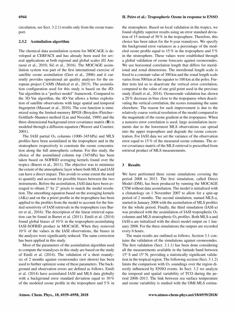
Figure 3 shows the comparison between the partial ozonecolumn of the three simulations and the ozonesonde data inthe tropical band (15◦ S–15◦ N). Partial ozone columns (inDU) and relative differences (in %) are plotted separatelyfor the TCO (1000–100 hPa), the boundary layer (1000–750 hPa) and the free troposphere (750–100 hPa). The TCOfrom ozonesondes (Fig. 3a) has maxima in summer–fall andminima in winter. The observed seasonal variation is a con-sequence of biomass burning, which provides precursors forozone formation in summer–fall. The emission of gases bybiomass burning, such as carbon monoxide and carbona-ceous aerosols, intensifies during the dry season (June–Julyand August–October) over both the South American andSouth African regions (Andreae et al., 1998; Sinha et al.,2004). The ozone columns produced by the DM and MLS-a simulations do not show the variability measured by theozonesondes; their correlation coefficients with the sondesdata are lower than 0.76 (Fig. 3a, b). The IASI-a variabilitymatches the ozonesondes better with a correlation coefficientof 0.88. In particular the IASI-a simulation exhibits a year-to-year variability that agrees very well with the ozonesondedata. This is confirmed by the RSD of the differences be-tween simulated and observed values: the RSD of IASI-a is6 % whereas it is about 10 % for MLS-a and MD. The rel-ative differences between simulated and observed values arepresented in Fig. 3b. IASI-a is less biased (6 %) than DM andMLS-a, and MLS-a has lower biases (24 %) than DM (32 %).Biases are lower with MLS-a, compared to DM, due to theassimilation of MLS stratospheric data. The MLS-a improve-ment is due to the direct influence of the lowest assimilated

level of MLS (170 hPa) which brings information on the O3distribution in the UTLS region. Compared to IASI-a thelower accuracy of DM comes from the use of the simplifiedozone scheme, which does not account for the production oftropospheric ozone by biomass burning.

Figure 3c and d show that the IASI-a tropospheric columnsare biased high in the lower troposphere. In this region, theRSDs of the three simulations are very similar, implying asimilar variability compared to ozonesondes, even if IASI-a matches the ozonesondes slightly better. However, IASI-ais half as accurate for the boundary layer O3 column thanfor the TCO and its biases are higher than MD and MLS-a. Larger biases in the boundary layer are a consequence ofboth the low degrees of freedom of IASI retrievals in thetroposphere and the presence of a DM bias with oppositesign between the free troposphere and the boundary layer.The positive correction provided by IASI assimilation in thefree troposphere propagates downward in the boundary layer,therefore increasing the original DM bias.

Ozone concentration and biases of the IASI-a simulationin the free troposphere (Fig. 3e and Fig. 3f) show much bet-ter results than the two other simulations. As can be seen,the sensitivity of the IASI measurements is larger in the mid-and upper troposphere. The RSD of IASI-a is around 6 %instead of 11 % for DM and 9 % for MLS-a in the middle–upper troposphere (Fig. 3f). The added value of IASI datain the middle troposphere is particularly remarkable in thecase of bias, which is 2 % for IASI-a instead of 41 and 32 %for DM and MLS-a, respectively. Since the boundary layer(1000–750 hPa) corresponds approximately to 12 % of theTCO (1000–100 hPa), the overestimation of the ozone col-umn by IASI-a does not have a major impact on the TCOused for our study of the ENSO-O3 correlation, which is themain objective of this study.

3.1.2 From eastern Africa to South America: focus onthe ENSO

To study the ENSO we divide the region of interest (latituderanges from 15◦ S to 15◦ N and longitude ranges from 70◦ Eto 110◦W) in two areas (see Fig. 2): the first one, called IIO,has a longitude range between 70 and 140◦E while the sec-ond one, called POC, is located between 180 and 110◦W.Three ozonesonde stations are available for both regions, twoin the IIO region and one in the POC region (Table 1).

Ozone measurements for each site are available over dif-ferent time periods. The Malaysia site provides measure-ments only between January 2008 and December 2009, theIndonesia site from January 2008 to December 2012, and theSamoa site from January 2008 to December 2013. Due tothe small number of ozonesonde measurements, results ofthe statistical validation presented here should be consideredwith more caution than in the previous section. The main ob-jective of this section is to check whether the reanalysis cancapture strong local variations of TCO due to ENSO.

www.atmos-chem-phys.net/18/6939/2018/ Atmos. Chem. Phys., 18, 6939–6958, 2018

6946 H. Peiro et al.: Tropospheric Ozone in response to ENSO

Figure 3. Time series of partial ozone columns (a, c, e, in DU) from the IASI-a (red curves), the MLS-a (blue curve), and the DM (greencurve) plotted versus several stations measurements from WOUDC (black curves). Data are 2-month averages over the area 15◦ S–15◦ N and180◦W–180◦ E for (a), the ozone column between 1015 and 100 hPa (b), the boundary layer (1015–750 hPa) (c), (d) and the free troposphere(750–100 hPa) (e), (f). Biases in percentages are shown in (a), (c) and (e). Mean biases, correlation coefficients and standard deviations arealso given (between brackets in b, d and f).

Table 1. Ozonesonde stations at tropical latitudes between 70◦ E and 110◦W.

Name Ozonesondes Localization Coordinates

Malaysia 443 ECC Kuala Lumpur international airport, Malaysia 3◦ N–101◦ EIndonesia 437 ECC Watukosek, Java Timur, Indonesia 8◦ S–113◦ ESamoa 191 ECC Apia, Samoa 13◦ S–172◦W

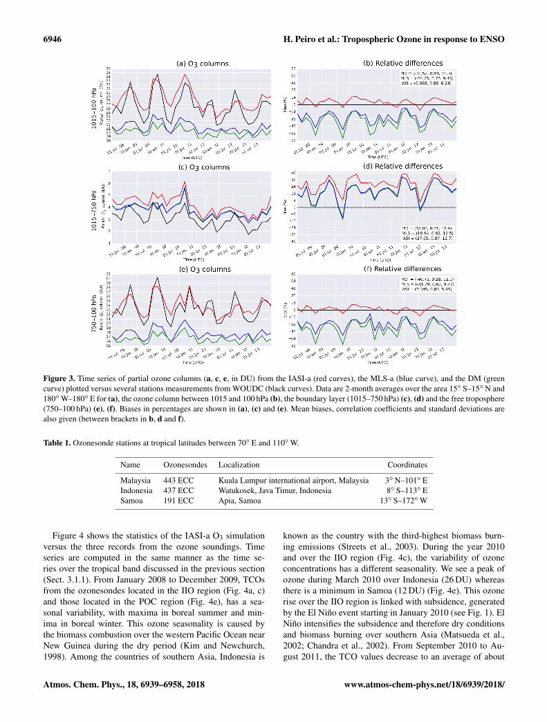
Figure 4 shows the statistics of the IASI-a O3 simulationversus the three records from the ozone soundings. Timeseries are computed in the same manner as the time se-ries over the tropical band discussed in the previous section(Sect. 3.1.1). From January 2008 to December 2009, TCOsfrom the ozonesondes located in the IIO region (Fig. 4a, c)and those located in the POC region (Fig. 4e), has a sea-sonal variability, with maxima in boreal summer and min-ima in boreal winter. This ozone seasonality is caused bythe biomass combustion over the western Pacific Ocean nearNew Guinea during the dry period (Kim and Newchurch,1998). Among the countries of southern Asia, Indonesia is

known as the country with the third-highest biomass burn-ing emissions (Streets et al., 2003). During the year 2010and over the IIO region (Fig. 4c), the variability of ozoneconcentrations has a different seasonality. We see a peak ofozone during March 2010 over Indonesia (26 DU) whereasthere is a minimum in Samoa (12 DU) (Fig. 4e). This ozonerise over the IIO region is linked with subsidence, generatedby the El Niño event starting in January 2010 (see Fig. 1). ElNiño intensifies the subsidence and therefore dry conditionsand biomass burning over southern Asia (Matsueda et al.,2002; Chandra et al., 2002). From September 2010 to Au-gust 2011, the TCO values decrease to an average of about

Atmos. Chem. Phys., 18, 6939–6958, 2018 www.atmos-chem-phys.net/18/6939/2018/

H. Peiro et al.: Tropospheric Ozone in response to ENSO 6947

20 DU over Indonesia. This decrease in tropospheric ozone isdue to the other phase of ENSO: La Niña. As we have alreadymentioned (Fig. 1), La Niña strengthens the convection overthe IIO causing a minimum in the TCO. Hence, there is alower TCO over Indonesia (around 20 DU) than over Samoa(around 28 DU). After summer 2011 the ENSO disappearsand the TCO returns to normal seasonality.

IASI-a reproduces quite well the variability measured bythe ozonesondes during normal conditions of the Walker cir-culation (2008–2009) and during the ENSO (2010–2011). Inparticular, IASI-a agreement with the ozonesondes is betterover the POC region (Samoa), where the correlation coef-ficient is 0.96, than over Indonesia and Malaysia where thecoefficients are around 0.7. However, the relative differencebetween IASI-a and the ozonesondes is larger over the POCregion (Fig. 4f) than over the IIO region (Fig. 4b, d), withan overestimation of the ozone columns by about 17 % inSamoa. Mean biases are around 3–5 % for over Indonesiaand Malaysia, showing that IASI-a reproduces quite well theozone variability during normal conditions of the Walker cir-culation. Equally, IASI-a reproduces the maximum over In-donesia and the minimum over Samoa during the 2010 ElNiño event, as well as the TCO minima generated during LaNiña over the IIO region. As already discussed, biases ob-served in the POC and IIO regions come from the decreasedsensitivity of IASI in the boundary layer, and from the lackof adequate representation of the chemistry in the lower tro-posphere by the linear scheme used within MOCAGE. Thethree simulations (IASI-a, MD and MLS-a) have identical bi-ases in the boundary layer compared to the ozone soundings(figures not shown). Biases in the boundary layer are higherin the POC region (around 45 %) compared to the IIO region(around 20 %). However, in the POC region, the variability ofthe three simulations are remarkably well correlated with theozonesondes, with coefficient correlations higher than 0.85(not shown).

To summarize, the IASI-a simulation reproduces well theO3 variability observed with the ozonesondes for the tropicallatitudes and for both regions of POC and IIO. The seasonaloscillations of ozone, caused by the anthropogenic pollutionand by ENSO, are reproduced by IASI-a despite a slightoverestimation of about 4 % in the IIO region and around17 % in the POC region. The IASI-a simulation is thus ad-equate to study ozone variability during ENSO events sincebiases are not very large over the period under study.

3.2 Temporal and spatial variability of ozone duringENSO

3.2.1 Characterization of ENSO and footprints on SSTand tropospheric ozone content

In this section we consider the link between SST and tro-pospheric ozone during ENSO events. Previous studies havehighlighted the link between SST anomalies and ENSO dy-

namics (Philander, 1989; Barnston et al., 1997; Wang et al.,2014). Colder SST in the POC region is associated with LaNiña whereas El Niño has warmer SST than under normalconditions (Trenberth, 1997). Variations in TCO concentra-tions are a combination of biomass burning rejecting largequantities of ozone precursors (Chandra et al., 2002) and aneastward shift in the tropical convection of the Walker cir-culation associated with SST changes (Chandra et al., 1998;Sudo and Takahashi, 2001a). The correlation between SSTand TCO have already been characterized using OMI-MLSdata; our objective is to see if similar correlations can bederived using the model simulations. To this end, we havetaken SST data from the Giovanni Interactive Visualizationand Analysis GES DISC: Goddard Earth Sciences, data andInformation Services Centre (https://disc.gsfc.nasa.gov). TheSST data were measured by the instrument MODIS (Moder-ate Resolution Imaging Spectroradiometer) aboard the Aquasatellites (NASA Earth Observing System platforms).

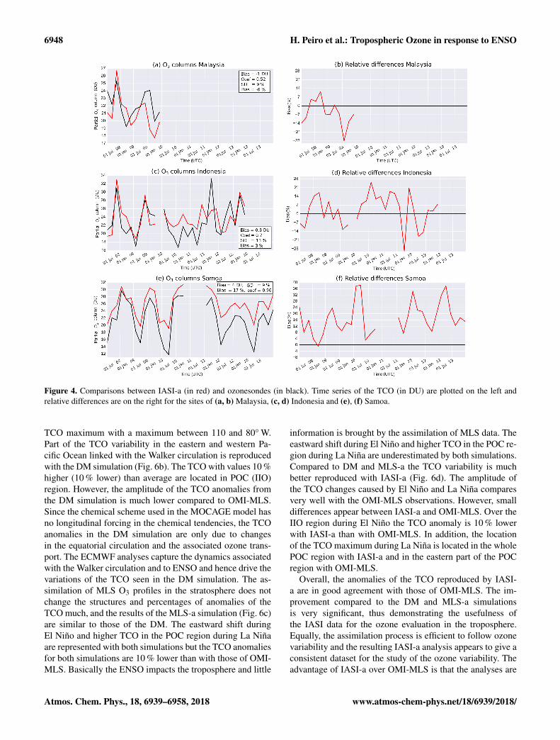
Figure 5 shows the time versus longitude Hovmöller di-agram, averaged between 15◦ S and 15◦ N, of the monthlymean SST and the OMI-MLS measurements. SST over thePacific ocean has a characteristic geographic distribution(Fig. 5a), with the warmest water in the IIO region (70–140◦ E) and coldest water in the POC region (180–110◦W).The link between SST and TCO (Chandra et al., 1998, 2009)is observed comparing the SST (Fig. 5a) with OMI-MLSmeasurements (Fig. 5b). The warmest water-induced con-vective movements result in a TCO decrease and vice versafor the coldest water. During El Niño (January 2010) thewarm SST shifts from the IIO region to the POC region.These eastward shifts in SST coincide with eastward shiftsof TCO from July 2008 to January 2010. During La Niña(occurred between September 2010 and January 2011) anopposite condition occurs with the strengthening of colderSST between 80 and 150◦W. In this region of colder SST(Fig. 5a), higher TCO (26–32 DU) is located between thecoast of South America and 140◦W (Fig. 5b). The eastwardshift of SST occurring from January 2011 to December 2013corresponds to the return of normal conditions over the Pa-cific ocean and impacts TCO with an eastward shift.

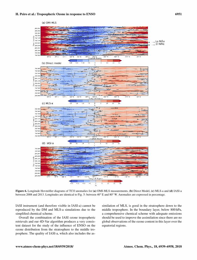
To compare the three model simulations, with OMI-MLS,we have computed anomalies of tropospheric ozone of eachdataset for the period 2008–2013 (Fig. 6). The anomaliesare calculated by subtracting the time-averaged TCO to eachTCO determination and this difference has been divided bythe mean TCO. The TCO anomalies are expressed in per-centage. The variability of TCO, observed previously withOMI-MLS measurements in Fig. 5, is also clearly visiblewith the TCO anomaly (Fig. 6a). The TCO with values 20 %lower than average are located in the IIO region. The TCOwith values 20 % higher than average are located close toSouth American coasts. The El Niño event on January 2010has a significant impact on TCO, with 20 % higher values inthe IIO region and 10 % lower in the POC region. The LaNiña event that follows shows different localization on the

www.atmos-chem-phys.net/18/6939/2018/ Atmos. Chem. Phys., 18, 6939–6958, 2018

6948 H. Peiro et al.: Tropospheric Ozone in response to ENSO

Figure 4. Comparisons between IASI-a (in red) and ozonesondes (in black). Time series of the TCO (in DU) are plotted on the left andrelative differences are on the right for the sites of (a, b) Malaysia, (c, d) Indonesia and (e), (f) Samoa.

TCO maximum with a maximum between 110 and 80◦W.Part of the TCO variability in the eastern and western Pa-cific Ocean linked with the Walker circulation is reproducedwith the DM simulation (Fig. 6b). The TCO with values 10 %higher (10 % lower) than average are located in POC (IIO)region. However, the amplitude of the TCO anomalies fromthe DM simulation is much lower compared to OMI-MLS.Since the chemical scheme used in the MOCAGE model hasno longitudinal forcing in the chemical tendencies, the TCOanomalies in the DM simulation are only due to changesin the equatorial circulation and the associated ozone trans-port. The ECMWF analyses capture the dynamics associatedwith the Walker circulation and to ENSO and hence drive thevariations of the TCO seen in the DM simulation. The as-similation of MLS O3 profiles in the stratosphere does notchange the structures and percentages of anomalies of theTCO much, and the results of the MLS-a simulation (Fig. 6c)are similar to those of the DM. The eastward shift duringEl Niño and higher TCO in the POC region during La Niñaare represented with both simulations but the TCO anomaliesfor both simulations are 10 % lower than with those of OMI-MLS. Basically the ENSO impacts the troposphere and little

information is brought by the assimilation of MLS data. Theeastward shift during El Niño and higher TCO in the POC re-gion during La Niña are underestimated by both simulations.Compared to DM and MLS-a the TCO variability is muchbetter reproduced with IASI-a (Fig. 6d). The amplitude ofthe TCO changes caused by El Niño and La Niña comparesvery well with the OMI-MLS observations. However, smalldifferences appear between IASI-a and OMI-MLS. Over theIIO region during El Niño the TCO anomaly is 10 % lowerwith IASI-a than with OMI-MLS. In addition, the locationof the TCO maximum during La Niña is located in the wholePOC region with IASI-a and in the eastern part of the POCregion with OMI-MLS.

Overall, the anomalies of the TCO reproduced by IASI-a are in good agreement with those of OMI-MLS. The im-provement compared to the DM and MLS-a simulationsis very significant, thus demonstrating the usefulness ofthe IASI data for the ozone evaluation in the troposphere.Equally, the assimilation process is efficient to follow ozonevariability and the resulting IASI-a analysis appears to give aconsistent dataset for the study of the ozone variability. Theadvantage of IASI-a over OMI-MLS is that the analyses are

Atmos. Chem. Phys., 18, 6939–6958, 2018 www.atmos-chem-phys.net/18/6939/2018/

H. Peiro et al.: Tropospheric Ozone in response to ENSO 6949

fully four-dimensional with 6-hourly outputs and resolvedinformation on the vertical dimension. The vertical distribu-tions are studied in Sect. 3.2.3.

3.2.2 Intercomparison of Ozone ENSO Indices

The OEI is the TCO difference computed between the IIOregion (70–140◦ E) and the POC region (180–110◦W). Theresulting time series are then deseasonalized. This deseason-alization is done to remove the signal of the annual cycle(Ziemke et al., 2010). OEI is a strong indicator of the ENSOintensity influencing the tropospheric ozone over IIO andPOC regions (Ziemke et al., 2010). It is considered as a ba-sic diagnostic tool to evaluate the ability of the models toreproduce changes in tropospheric ozone linked with ENSO(Ziemke et al., 2010, 2014).

Figure 7 shows the OEI during the period January 2008to December 2013 computed from our model analyses andfrom the OMI-MLS data. The OEI variations are related toENSO, with maxima during El Niño and minima during LaNiña events. In Fig. 7a we have plotted the OEI computedfor the OMI-MLS measurements (noted OMI-MLS) and theNiño 3.4 index. The monthly Niño 3.4 is calculated from SSTanomalies in the Pacific Ocean. The Niño 3.4 index calcu-lated from SST is available from the NOAA website (http://www.cpc.ncep.noaa.gov/data/indices/). Sea surface temper-ature anomalies were calculated using the monthly Ex-tended Reconstructed Sea Surface Temperature version 4(ERSST.v4, 1950–2016 base period). Also included is theOEI of OMI-MLS smoothed using a 3-month running aver-age, as computed by Ziemke et al. (2010, 2014) and calledOEI-Z hereafter. Figure 7b shows the OEI computed fromIASI-a, MLS-a, DM and OMI-MLS. Our OEI indices fromOMI-MLS, DM, MLS-a and IASI-a are computed withouttime averaging, by subtraction of TCO in the POC regionfrom TCO averaged over the IIO region. As defined by theNOAA, the two ENSO phases occur when the Niño 3.4 in-dex is higher than 0.5 (corresponding to El Niño) and lowerthan −0.5 (corresponding to La Niña) during five consecu-tive months. Thus, in the analyzed period an El Niño startson July 2008 with a maximum on January 2010, and a LaNiña starts on July 2010 with a maximum on January 2011.The two time series of OEI-Z and OMI-MLS appear remark-ably similar (Fig. 7a), except around January 2008. For thisperiod they are out of phase with the Niño 3.4. The discrep-ancy is attributed to the phase opposition between the in-terannual and intraseasonal variability of the TCO (Ziemkeet al., 2014) linked with the intraseasonal Madden–Julian Os-cillation (MJO, Madden and Julian, 1972, 1994). The MJOincreases the differences between OEI-Z and OMI-MLS in2008. Detailing the effect of MJO on monthly OEI is be-yond the scope of our current study. As expected, the OEIfrom OMI-MLS shows a consistent variability with OEI-Z;in particular the maxima and minima agree and are well cor-related to the Niño 3.4 index. Since the OMI-MLS OEI is

obtained from monthly averages it exhibits shorter term vari-ability than OEI-Z and can be directly compared to the in-dices derived from the model simulations.

The DM OEI (Fig. 7b, green curve) is negative during thewhole period, corresponding to a tropospheric column higherover the POC region than over the IIO region. The DM OEIvariations show some features of the ENSO, with a relativemaximum in January 2010 followed by a minimum at theend of the same year, but the intensity is weak: about 3 timeslower than values observed with OMI-MLS. The MLS-a pro-duces an OEI very similar to DM. As already discussed, con-straining the ozone profile in the stratosphere has little im-pact on the quality of the modeled ENSO O3 signal. Withthe IASI-a we can quantify the contribution of IASI data inthe computed OEI (Fig. 7b, red curve). Compared to DMand MLS-a simulations the IASI-a analysis produces OEI inbetter agreement with the ones derived from OMI-MLS. TheOEI variations are in phase with a very good match of pe-riods of maxima and minima. There is, however, a constantbias of approximately 2.4 DU between the indices of OMI-MLS and IASI-a. As discussed in Sect. 3.1.2, IASI-a biasin the lower troposphere is larger in the POC region than inthe IIO region. This difference of biases between POC andIIO regions affects the determination of the OEI. In addition,during ENSO events we have seen from the Hovmöller plotsin Sect. 3.2.1 that during La Niña the TCO maximum withIASI-a is slightly shifted to the western part of the POC re-gion compared to the OMI-MLS data. The difference in thelocation of maxima over the eastern Pacific between OMI-MLS and IASI-a explains part of the difference in the OEIabsolute values during El Niño and La Niña events (Fig. 7).

Tropospheric ozone variability during ENSO is thereforevery well captured from the OEI variations computed fromIASI-a, despite a constant bias in the boundary layer. Furtherinsights into the vertical distribution of O3 over the POC andIIO regions during ENSO are discussed in the next section.

3.2.3 Vertical structure of O3

The evaluations of TCO obtained with the OMI-MLS by sub-tracting stratospheric ozone from MLS from the total ozonefrom OMI cannot give information on the vertical structureof the O3 anomalies forced by ENSO. This is clearly anadvantage of model assimilations that can give a completethree-dimensional structure of the ozone fields with no gapsdue to orbitography and clouds. We focus here on the infor-mation brought by the assimilation of IASI and MLS datain describing the vertical ozone response to ENSO in thePOC and IIO regions. Figure 8 shows monthly mean ozoneprofiles for IASI-a, MLS-a and DM, over the 6-year record.The tropopause pressure for the three simulations is about100 hPa. Ozone concentration in this layer is around 70 ppbv.Due to the limitations of the model and the lack of informa-tion brought by the two instruments in the boundary layer, as

www.atmos-chem-phys.net/18/6939/2018/ Atmos. Chem. Phys., 18, 6939–6958, 2018

6950 H. Peiro et al.: Tropospheric Ozone in response to ENSO

Figure 5. (a) Time versus longitude Hovmöller diagram of the SST (in ◦C). (b) Same diagram from the OMI-MLS data. The data aremonthly means from January 2008 to December 2013 and area-averaged between latitudes 15◦ S and 15◦ N. Also included on the bottomare the corresponding maps of the Hovmöller diagram.

already discussed, we focus our analysis in the IIO et POCregions on the free troposphere, between 750 and 100 hPa.

The DM (Fig. 8a, b) and MLS-a (Fig. 8c, d) produce veryclose distributions of the vertical ozone concentration. TheMLS-a simulation shows slightly more ozone in the lowerstratosphere and upper troposphere, but the fluctuations ofthe concentration have similar amplitudes in both simula-tions. Particularly noticeable is the signal during the 2010El Niño with low ozone values in the POC region duringthe first months of the year linked to increased convectionand associated upward motions, and an opposite behavior inthe IIO region with subsidence and increased ozone downto the middle troposphere. This footprint of ENSO is verywell captured with the IASI-a simulation, especially over thePOC region. Over that region the ozone content is lower than35 ppbv during El Niño and larger than 50 ppbv during LaNiña. The information brought by IASI is very significant,the amplitude of the ozone change between El Niño and La

Niña periods is 2 to 3 times larger with IASI-a assimilationthan it is with DM and MLS-a simulations. If we refer to OEIindices (Fig. 7) some ENSO activity is detected in late 2012–early 2013. Indeed an O3 minimum in early 2013 followedby a maximum in the middle of the year is clearly visible inthe IASI-a assimilation in the POC region. The amplitude ofthe ENSO signal on ozone is lower than for the 2010 event,in agreement with the lower values of the Niño 3.4 index.Also more clearly visible with IASI-a are the seasonal vari-ations of the ozone content in the IIO region that is quiteregular outside ENSO periods. In that region the annual pe-riodicity of ozone is much pronounced in comparison to themore erratic variations shown in the POC region. The regu-larity of the ozone fluctuation is more pronounced in IASI-aassimilation than in DM and MLS-a simulations. In additionto the influence of atmospheric dynamics, biomass burningand the associated ozone production could trigger the sea-sonal fluctuations. Such an ozone production detected by the

Atmos. Chem. Phys., 18, 6939–6958, 2018 www.atmos-chem-phys.net/18/6939/2018/

H. Peiro et al.: Tropospheric Ozone in response to ENSO 6951

Figure 6. Longitude Hovmöller diagrams of TCO anomalies for (a) OMI-MLS measurements, (b) Direct Model, (c) MLS-a and (d) IASI-abetween 2008 and 2013. Longitudes are identical to Fig. 5: between 40◦ E and 80◦W. Anomalies are expressed in percentage.

IASI instrument (and therefore visible in IASI-a) cannot bereproduced by the DM and MLS-a simulations due to thesimplified chemical scheme.

Overall the combination of the IASI ozone troposphericretrievals and our 4D-Var algorithm produces a very consis-tent dataset for the study of the influence of ENSO on theozone distribution from the stratosphere to the middle tro-posphere. The quality of IASI-a, which also includes the as-

similation of MLS, is good in the stratosphere down to themiddle troposphere. In the boundary layer, below 800 hPa,a comprehensive chemical scheme with adequate emissionsshould be used to improve the assimilation since there are noglobal observations of the ozone content in this layer over theequatorial regions.

www.atmos-chem-phys.net/18/6939/2018/ Atmos. Chem. Phys., 18, 6939–6958, 2018

6952 H. Peiro et al.: Tropospheric Ozone in response to ENSO

Figure 7. (a) Monthly mean tropospheric Ozone ENSO Index (in DU) derived from the OMI-MLS data (grey line). Also shown is theNiño 3.4 monthly temperature anomaly ENSO index (cyan curve, multiplied by a factor of 3, in Kelvin) and the OEI-Z index derived fromthe OMI-MLS data with a deseasonalization followed by a sliding average of 3 months (orange curve). (b) The OMI-MLS data (grey curve)as in the above plot, the MLS-a (in blue curve), the DM in green curve and the IASI-a (in red curve). All ENSO indices extend fromJanuary 2008 through December 2013.

4 Summary and conclusion

A total of 6 years (from January 2008 to December 2013)of 6-hourly tropospheric ozone fields have been derivedby assimilating IASI and MLS ozone measurements in theMOCAGE CTM. The assimilation of IASI troposphericcolumns combined with MLS stratospheric profiles was firstvalidated against ozonesondes in the tropical band (15◦ S–15◦ N), providing a statistically robust validation. In the trop-ical band and over the whole period, IASI-a gives results sim-ilar to ozonesondes and reproduces the ozone variability welldespite a constant bias. Biases in the analysis come from thelow accuracy of the model in the boundary layer. The ozonelinear scheme in MOCAGE does not take surface emissionsinto account. In addition, IASI has a weak sensitivity in theboundary layer and therefore does not provide additional in-formation on O3 content in this layer. A second validationhas been done over the Pacific ocean and over southern Asia

(longitude band of 70◦ E to 110◦W). During the 2008–2013period, an ENSO event developed with its two phases: ElNiño in winter 2010 and La Niña in winter 2011. IASI-a hasbeen validated in two areas: the Indonesia and Indian Oceanand the Pacific Ocean Center regions. In both regions, biasesappear and are larger in the POC region. The weak sensitiv-ity of IASI sounding in the boundary layer is responsible forthese biases. However, the tropospheric ozone variability re-lated to the Walker Circulation and to the ENSO event is wellreproduced with IASI-a.

OMI-MLS tropospheric columns have been used and val-idated by several past studies. We have used OMI-MLSozone data to characterize the links between SST and tro-pospheric O3 and to compare with our IASI-a assimilation.Anomalies of TCO have been computed, allowing a compar-ison between IASI-a and the two other simulations (DirectModel and MLS-a) with OMI-MLS. Anomalies of the Di-rect Model (MOCAGE without assimilation) are similar to

Atmos. Chem. Phys., 18, 6939–6958, 2018 www.atmos-chem-phys.net/18/6939/2018/

H. Peiro et al.: Tropospheric Ozone in response to ENSO 6953

Figure 8. Monthly mean time series of ozone vertical profiles (units ppbv) versus pressure for the IIO region (a, c, e) and the POC region (b,d, f). The abscissa goes from January 2008 to December 2013. Panels (a, b) correspond to the Direct Model, (c, d) to the MLS-a and (e, f)to the IASI-a simulations. Pressure scale goes from 1013 to 20 hPa.

anomalies of MLS-a (assimilation of MLS stratospheric pro-files). The good reproduction of anomalies in terms of loca-tion and timing between eastern and western regions in bothsimulations are due to the transport forced by the winds fromthe ECMWF meteorological analyses. However, the ampli-tude of anomalies is lower than in OMI-MLS data. Assimi-lation of IASI data corrects this behavior, and the anomaliesof IASI-a appear very similar to the OMI-MLS anomalies. Inparticular, the IASI data bring essential information to repro-duce the eastward shift of TCO caused by El Niño.

In order to study the ability of IASI-a to reproduce theozone variability caused by El Niño and La Niña phases, wehave used the OEI. The OEI represents an essential diagnos-tic test for models that should be able to represent ozone fea-tures linked with ENSO changes in tropospheric dynamics.

OEI from IASI-a shows variations similar to those of OMI-MLS with a small bias corresponding to higher TCO over thePOC than over the IIO region. The Direct Model and MLS-ahave the same bias. This bias has been located in the bound-ary layer with the comparison with the ozonesondes.

We have also examined the vertical structures of tropo-spheric ozone in the IIO and POC regions, with the threesimulations (Direct Model, MLS-a and IASI-a), in order toshow the contribution of IASI tropospheric data in the as-similation. The IASI-a analysis is consistent with the ozonedisplacements in adequation with subsidences and conver-gences generated by El Niño and La Niña in both IIO andPOC regions. The IASI assimilation gives a very valuablehigh-resolution dataset suitable to perform analyses of the

www.atmos-chem-phys.net/18/6939/2018/ Atmos. Chem. Phys., 18, 6939–6958, 2018

6954 H. Peiro et al.: Tropospheric Ozone in response to ENSO

O3 variability in the upper and middle troposphere for short-term and interannual timescales in the tropical band.

Overall, the assimilation of stratospheric MLS and tropo-spheric IASI data within MOCAGE gives a good representa-tion of the tropospheric ozone variability linked with ENSOand the Walker circulation. We have shown the importance ofassimilating tropospheric IASI data to provide vertical infor-mation on tropospheric ozone variability, showing the benefitof IASI analyses for studies on ENSO dynamics. In addition,since ENSO is one of the most important interannual fluc-tuations in climate variability, this study is part of a climatevariability perspective. The assimilation of satellite data ispromising for determining the impact of climate variabilityon tropospheric chemistry. There are, however, some limi-tations in our simulations that have to be addressed. One ofthem is the bias found in the boundary layer over the PacificOcean that affects the calculation of the OEI. In this studywe have used a linear ozone parameterization to compute theozone chemical tendencies. This approach is suitable for thefree troposphere and the stratosphere but is certainly not ad-equate for the boundary layers. In the future we plan to use amore comprehensive chemical scheme that accounts for thesurface emissions.

With the use of IASI data we have demonstrated herethe value of assimilating satellite data that document the di-rect information in the tropospheric ozone content to com-pute OEI. This approach is promising because many types ofdata can enter in an assimilation process, such as the bal-loon and aircraft measurements. Improvements in the tro-pospheric ozone content evaluations can be expected froman increase in assimilated data. Times series of IASI analy-sis could then be derived and used to study the troposphericozone variability over at least a 30-year period. One advan-tage of infrared sounders like IASI for climate studies is theirgood spectral stability over time, with respect for example toUV instruments. This is an important feature when trying todetermine potentially small climate signals hidden by largeozone variability, due for example to ENSO. Finally, using amore detailed chemistry scheme within future ozone reanaly-ses would also allow further insights into chemical feedbacksin the context of a changing climate.

Data availability. IASI L1 data were provided by the Labora-tory of Aerology. EOS MLS L2 version 4 is available at https://mls.jpl.nasa.gov/data/. The OMI-MLS tropospheric ozone as wellas the OEI-Z index are available at http://acd-ext.gsfc.nasa.gov/Data_services/cloud_slice/. The Nino3.4 index is available from theNOAA website at http://www.cpc.ncep.noaa.gov/data/indices/.

Competing interests. The authors declare that they have no conflictof interest.

Acknowledgements. We would like to thank Jerry R. Ziemkeand the Aura Ozone Monitoring Instrument (OMI) science teamof the NASA Goddard Space Flight Center to the availabilityof the OMI-MLS data and the OEI-Z Index. We also thankWOUDC for providing ozonesonde station data and the NASAJet Propulsion Laboratory for the availability of Aura MLS data.We also acknowledge the mission scientists from the NASAGES DISC, who provided the GIOVANNI SST data used in thisresearch. In addition, we acknowledge la Région Midi-Pyrénéesfor financial support and the CNES (Centre National d’ÉtudesSpatiales) for financial sources on the TOSCA project. Thanks alsoto Sean Crowell for proofreading an earlier version of this paper.

Edited by: Jayanarayanan KuttippurathReviewed by: Catherine Wespes and one anonymous referee

References

Andreae, M. O., Andreae, T. W., Annegarn, H., Beer, J., Cachier,H., Canut, P. L., Elbert, W., Maenhaut, W., Salma, I., Wienhold,F. G., and Zenker, T.: Airborne studies of aerosol emissions fromsavanna fires in southern Africa, J. Geophys. Res.-Space Phys.,103, 32119–32128, 1998.

Ardanuy, P. E. and Lee Kyle, H.: El Nino and Outgoing LongwaveRadiation: Observations from Nimbus-7 ERB, Am. Meteorol.Soc., 114, 415–433, 1985.

Barnston, A. G., Chelliah, M., and Goldenberg, S. B.: Documen-tation of a Highly ENSO-related SST region in the EquatorialPacific, Atmos. Ocean, 35, 367–383, 1997.

Barré, J., Peuch, V. H., Attié, J. L., El Amraoui, L., La-hoz, W. A., Josse, B., Claeyman, M., and Nédélec, P.:Stratosphere-troposphere ozone exchange from high resolutionMLS ozone analyses, Atmos. Chem. Phys., 12, 6129–6144,https://doi.org/10.5194/acp-12-6129-2012, 2012.

Barré, J., Peuch, V.-H., Lahoz, W. A., Attié, J.-L., Josse, B., Pi-acentini, A., Eremenko, M., Dufour, G., Nedelec, P., von Clar-mann, T., and El Amraoui, L.: Combined data assimilationof ozone tropospheric columns and stratospheric profiles in ahigh-resolution CTM, Q. J. Roy. Meteorol. Soc., 140, 966–981,https://doi.org/10.1002/qj.2176, 2013.

Barret, B., Le Flochmoen, E., Sauvage, B., Pavelin, E., Matricardi,M., and Cammas, J. P.: The detection of post-monsoon tropo-spheric ozone variability over south Asia using IASI data, At-mos. Chem. Phys., 11, 9533–9548, https://doi.org/10.5194/acp-11-9533-2011, 2011.

Barret, B., Sauvage, B., Bennouna, Y., and Le Flochmoen,E.: Upper-tropospheric CO and O3 budget during the Asiansummer monsoon, Atmos. Chem. Phys., 16, 9129–9147,https://doi.org/10.5194/acp-16-9129-2016, 2016.

Bell, M. L., McDermott, A., Zeger, S. L., Samet, J. M., and Do-minici, F.: Ozone and mortality in 95 US urban communities,1987 to 2000, JAMA, National Institutes of Health, 292, 2372–2378, https://doi.org/10.1001/jama.292.19.2372, 2004.

Berrisford, P., Dee, D. P., Poli, P., Brugge, R., Fielding, K., Fuentes,M., Kallberg, P. W., Kobayashi, S., Uppala, S., and Simmons, A.:The ERA-Interim archive Version 2.0, Shinfield Park, Reading,2–22, 2011.

Atmos. Chem. Phys., 18, 6939–6958, 2018 www.atmos-chem-phys.net/18/6939/2018/

H. Peiro et al.: Tropospheric Ozone in response to ENSO 6955

Bousserez, N., Attié, J. L., Peuch, V. H., Michou, M., Pfister,G., Edwards, D., Emmons, L., Mari, C., Barret, B., Arnold,S. R., Heckel, A., Richter, A., Schlager, H., Lewis, A., Avery,M. A., Sachse, G. W., Browell, E. V., and Hair, J. W.: Eval-uation of the MOCAGE chemistry transport model during theICARTT/ITOP experiment, J. Geophys. Res.-Atmos., 112, 1–18,https://doi.org/10.1029/2006JD007595, 2007.

Cariolle, D. and Teyssèdre, H.: A revised linear ozone photochem-istry parameterization for use in transport and general circulationmodels: multi-annual simulations, Atmos. Chem. Phys., 7, 2183–2196, https://doi.org/10.5194/acp-7-2183-2007, 2007.

Chandra, S., Ziemke, J. R., Min, W., and Read, W. G.:Effects of 1997–1998 El Nino on tropospheric ozoneand water vapor, Geophys. Res. Lett., 25, 3867–3870,https://doi.org/10.1029/98gl02695, 1998.

Chandra, S., Ziemke, J. R., Barthia, P. K., and Martin,R. V.: Tropical tropospheric ozone: Implications for dy-namics and biomass burning, J. Geophys. Res., 107,https://doi.org/10.1029/2001JD000447, 2002.

Chandra, S., Ziemke, J. R., Duncan, B. N., Diehl, T. L., Livesey,N. J., and Froidevaux, L.: Effects of the 2006 El Niño on tro-pospheric ozone and carbon monoxide: implications for dynam-ics and biomass burning, Atmos. Chem. Phys., 9, 4239–4249,https://doi.org/10.5194/acp-9-4239-2009, 2009.

Clerbaux, C., Boynard, A., Clarisse, L., George, M., Hadji-Lazaro,J., Herbin, H., Hurtmans, D., Pommier, M., Razavi, A., Turquety,S., Wespes, C., and Coheur, P.-F.: Monitoring of atmosphericcomposition using the thermal infrared IASI/MetOp sounder, At-mos. Chem. Phys., 9, 6041–6054, https://doi.org/10.5194/acp-9-6041-2009, 2009.

Coheur, P.-F., Clarisse, L., Turquety, S., Hurtmans, D., and Cler-baux, C.: IASI measurements of reactive trace species inbiomass burning plumes, Atmos. Chem. Phys., 9, 5655–5667,https://doi.org/10.5194/acp-9-5655-2009, 2009.

Cooper, O. R., Parrish, D. D., Ziemke, J., Balashov, N. V., Cu-peiro, M., Galbally, I. E., Gilge, S., Horowitz, L., Jensen,N. R., Lamarque, J.-F., Naik, V., Oltmans, S. J., Schwab,J., Shindell, D. T., Thompson, a. M., Thouret, V., Wang, Y.,and Zbinden, R. M.: Global distribution and trends of tropo-spheric ozone: An observation-based review, Elementa, 2, 2–29,https://doi.org/10.12952/journal.elementa.000029, 2014.

Craig, R.-A.: The upper atmosphere, meteorology and physics, Aca-demic Press, 8, 23–25, 1965.

Curtis, S. and Adler, R.: ENSO indices based onpatterns of satellite-derived precipitation, J. Cli-mate, 13, 2786–2793, https://doi.org/10.1175/1520-0442(2000)013<2786:EIBOPO>2.0.CO;2, 2000.

Dobber, M. R., Dirksen, R. J., Levelt, P. F., Van Den Oord, G.H. J., Voors, R. H. M., Kleipool, Q., Jaross, G., Kowalewski,M., Hilsenrath, E., Leppelmeier, G. W., De Vries, J., Dierssen,W., and Rozemeijer, N. C.: Ozone monitoring instrumentcalibration, IEEE T. Geosci. Remote Sens., 44, 1209–1238,https://doi.org/10.1109/TGRS.2006.869987, 2006.

Doherty, R. M., Stevenson, D. S., Collins, W. J., and Sanderson,M. G.: Influence of convective transport on tropospheric ozoneand its precursors in a chemistry-climate model, Atmos. Chem.Phys., 5, 3205–3218, https://doi.org/10.5194/acp-5-3205-2005,2005.

Doherty, R. M., Stevenson, D. S., Johnson, C. E., Collins, W. J., andSanderson, M. G.: Tropospheric ozone and El Niño–SouthernOscillation: Influence of atmospheric dynamics, biomass burn-ing emissions, and future climate change, J. Geophys. Res., 111,1–21, https://doi.org/10.1029/2005JD006849, 2006.

Dufour, G., Eremenko, M., Orphal, J., and Flaud, J.-M.: IASIobservations of seasonal and day-to-day variations of tropo-spheric ozone over three highly populated areas of China: Bei-jing, Shanghai, and Hong Kong, Atmos. Chem. Phys., 10, 3787–3801, https://doi.org/10.5194/acp-10-3787-2010, 2010.

Dufour, G., Eremenko, M., Griesfeller, A., Barret, B.,LeFlochmoën, E., Clerbaux, C., Hadji-Lazaro, J., Coheur,P.-F., and Hurtmans, D.: Validation of three different scientificozone products retrieved from IASI spectra using ozonesondes,Atmos. Meas. Tech., 5, 611–630, https://doi.org/10.5194/amt-5-611-2012, 2012.

Ebi, K. L. and McGregor, G.: Climate change, tropospheric ozoneand particulate matter, and health impacts, Environ. HealthPerspect., 116, 1449–1455, https://doi.org/10.1289/ehp.11463,2008.

El Amraoui, L., Attié, J., Semane, N., Claeyman, M., Peuch,V., Warner, J., Ricaud, P., Cammas, J., Piacentini, A., andJosse, B.: Midlatitude stratosphere–troposphere exchange as di-agnosed by MLS O3 and MOPITT CO assimilated fields, At-mos. Chem. Phys., 10, 2175–2194, https://doi.org/10.5194/acp-10-2175-2010, 2010.

Emili, E., Barret, B., Massart, S., Le Flochmoen, E., Piacen-tini, A., El Amraoui, L., Pannekoucke, O., and Cariolle,D.: Combined assimilation of IASI and MLS observationsto constrain tropospheric and stratospheric ozone in a globalchemical transport model, Atmos. Chem. Phys., 14, 177–198,https://doi.org/10.5194/acp-14-177-2014, 2014.

EOS MLS L2 version 4, available at: https://mls.jpl.nasa.gov/data/,2017.

Fowler, D., Amann, M., Anderson, R., Ashmore, M., Cox, P., De-pledge, M., Derwent, D., Grennfelt, P., Hewitt, N., Hov, O.,Jenkin, M., Kelly, F., Liss, P., Pilling, M., Pyle, J., Slingo, J.,and Stevenson, D.: Ground-level ozone in the 21st century: fu-ture trends, impacts and policy implications, October, The RoyalSociety, report 15/08, 2008.

Froidevaux, L., Jiang, Y. B., Lambert, A., Livesey, N. J., Read,W. G., Waters, J. W., Browell, E. V., Hair, J. W., Avery, M. A.,McGee, T. J., Twigg, L. W., Sumnicht, G. K., Jucks, K. W., Mar-gitan, J. J., Sen, B., Stachnik, R. A., Toon, G. C., Bernath, P. F.,Boone, C. D., Walker, K. A., Filipiak, M. J., Harwood, R. S.,Fuller, R. A., Manney, G. L., Schwartz, M. J., Daffer, W. H.,Drouin, B. J., Cofield, R. E., Cuddy, D. T., Jarnot, R. F., Knosp,B. W., Perun, V. S., Snyder, W. V., Stek, P. C., Thurstans, R. P.,and Wagner, P. A.: Validation of Aura Microwave Limb Sounderstratospheric ozone measurements, J. Geophys. Res.-Atmos.,113, D15S20, https://doi.org/10.1029/2007JD008771, 2008.

Geer, A. J., Lahoz, W. A., Bekki, S., Bormann, N., Errera, Q., Es-kes, H. J., Fonteyn, D., Jackson, D. R., Juckes, M. N., Massart,S., Peuch, V. H., Rharmili, S., and Segers, A.: The ASSET inter-comparison of ozone analyses: Method and first results, Atmos.Chem. Phys., 6, 5445–5474, https://doi.org/10.5194/acp-6-5445-2006, 2006.

Guilbert, J. J.: The world health report 2002 – reducing risks, pro-moting healthy life., Education for health (Abingdon, England),

www.atmos-chem-phys.net/18/6939/2018/ Atmos. Chem. Phys., 18, 6939–6958, 2018

6956 H. Peiro et al.: Tropospheric Ozone in response to ENSO

16, p. 230, https://doi.org/10.1080/1357628031000116808,2003.

Herbin, H., Hurtmans, D., Clerbaux, C., Clarisse, L., and Coheur,P.-F.: H16

2 O and HDO measurements with IASI/MetOp, Atmos.Chem. Phys., 9, 9433–9447, https://doi.org/10.5194/acp-9-9433-2009, 2009.

Honoré, C., Rouïl, L., Vautard, R., Beekmann, M., Bessagnet,B., Dufour, A., Elichegaray, C., Flaud, J. M., Malherbe, L.,Meleux, F., Menut, L., Martin, D., Peuch, A., Peuch, V. H.,and Poisson, N.: Predictability of European air quality: As-sessment of 3 years of operational forecasts and analyses bythe PREV’AIR system, J. Geophys. Res.-Atmos., 113, D04301,https://doi.org/10.1029/2007JD008761, 2008.

Houghton, J. T., Ding, Y., Griggs, D. J., Noguer, M., Vander Linden, P. J., Dai, X., Maskell, K., and Johnson,C. A.: Climate Change 2001: The Scientific Basis, Cli-mate Change 2001: The Scientific Basis, 57, p. 881,https://doi.org/10.1256/004316502320517344, 2001.

Josse, B., Simon, P., and Peuch, V. H.: Radon global simulationswith the multiscale chemistry and transport model MOCAGE,Tellus B, 56, 339–356, https://doi.org/10.1111/j.1600-0889.2004.00112.x, 2004.

Kim, J. H. and Newchurch, M. J.: Biomass-burning influence ontropospheric ozone over New Guinea and South America, J. Geo-phys. Res., 103, 1455–1461, https://doi.org/10.1029/97JD02294,1998.

Lacis, A. A., Wuebbles, D. K., and Logan, J. A.: Radiative forc-ing of climate by changes in the vertical distribution of ozone, J.Geophys. Res, 95, 9971–9981, 1990.

Lee, S., Shelow, D. M., Thompson, A. M., and Miller,S. K.: QBO and ENSO variability in temperature and ozonefrom SHADOZ, 1998–2005, J. Geophys. Res., 115, D18105,https://doi.org/10.1029/2009JD013320, 2010.

Levelt, P. F., van den Oord, G. H. J., Dobber, M. R., Malkki, A.,Visser, H., de Vries, J., Stammes, P., Lundell, J. O. V., and Saari,H.: The ozone monitoring instrument, IEEE T. Geosci. RemoteSens., 44, 1093–1101, 2006.

Liu, D. C. and Nocedal, J.: On the limited memory BFGS methodfor large scale optimization, Math. Program., 45, 503–528,https://doi.org/10.1007/BF01589116, 1989.

Liu, J., Rodriguez, J. M., Steenrod, S. D., Douglass, A. R., Lo-gan, J. A., Olsen, M. A., Wargan, K., and Ziemke, J. R.: Causesof interannual variability over the southern hemispheric tropo-spheric ozone maximum, Atmos. Chem. Phys., 17, 3279–3299,https://doi.org/10.5194/acp-17-3279-2017, 2017.

Liu, X., Bhartia, P. K., Chance, K., Froidevaux, L., Spurr, R. J.D., and Kurosu, T. P.: Validation of Ozone Monitoring Instru-ment (OMI) ozone profiles and stratospheric ozone columnswith Microwave Limb Sounder (MLS) measurements, Atmos.Chem. Phys., 10, 2539–2549, https://doi.org/10.5194/acp-10-2539-2010, 2010.

Livesey, N. J., Read, W. G., Froidevaux, L., Lambert, A., Manney,G. L., Pumphrey, H. C., Santee, M. L., Schwartz, M. J., Wang,S., Cofield, R. E., Cuddy, D. T., Fuller, R. A., Jarnot, R. F., Jiang,J. H., Knosp, B. W., Stek, P. C., Wagner, P. A., and Wu, D. L.:EOS MLS Version 3.3 Level 2 data quality and description docu-ment, Technical Report, Jet Propulsion Laboratory, 1–162, 2011.

Livesey, N. J., Read, W. G., Wagner, P. A., Froidevaux, L., Lambert,A., Manney, G. L., Millan Valle, L. F., Pumphrey, H. C., Santee,

M. L., Schwartz, M. J., Wang, R. A., Fuller, R. F., Jarnot, B. W.,and Knosp, E. M.: EOS MLS Version 4.2× Level 2 data qualityand description document, Tech. rep., 120–130, 2016.

Madden, R. A. and Julian, P. R.: Description of Global-Scale Circulation Cells in the Tropics with a 40–50Day Period, 29, 1109–1123, https://doi.org/10.1175/1520-0469(1972)029<1109:DOGSCC>2.0CO;2, 1972.

Madden, R. A. and Julian, P. R.: Observations of the40–50-Day Tropical Oscillation – A review., Mon.Weather Rev., 122, 814–837, https://doi.org/10.1175/1520-0493(1994)122<0814:OOTDTO>2.0.CO;2, 1994.

Marécal, V., Peuch, V. H., Andersson, C., Andersson, S., Arteta,J., Beekmann, M., Benedictow, A., Bergström, R., Bessagnet,B., Cansado, A., Chéroux, F., Colette, A., Coman, A., Curier,R. L., Van Der Gon, H. A., Drouin, A., Elbern, H., Emili,E., Engelen, R. J., Eskes, H. J., Foret, G., Friese, E., Gauss,M., Giannaros, C., Guth, J., Joly, M., Jaumouillé, E., Josse,B., Kadygrov, N., Kaiser, J. W., Krajsek, K., Kuenen, J., Ku-mar, U., Liora, N., Lopez, E., Malherbe, L., Martinez, I., Melas,D., Meleux, F., Menut, L., Moinat, P., Morales, T., Parmen-tier, J., Piacentini, A., Plu, M., Poupkou, A., Queguiner, S.,Robertson, L., Rouïl, L., Schaap, M., Segers, A., Sofiev, M.,Tarasson, L., Thomas, M., Timmermans, R., Valdebenito, VanVelthoven, P., Van Versendaal, R., Vira, J., and Ung, A.: A re-gional air quality forecasting system over Europe: The MACC-IIdaily ensemble production, Geosci. Model Dev., 8, 2777–2813,https://doi.org/10.5194/gmd-8-2777-2015, 2015.

Massart, S., Clerbaux, C., Cariolle, D., Piacentini, A., Turquety, S.,and Hadji-Lazaro, J.: First steps towards the assimilation of IASIozone data into the MOCAGE-PALM system, Atmos. Chem.Phys., 9, 5073–5091, https://doi.org/10.5194/acp-9-5073-2009,2009.

Massart, S., Pajot, B., Piacentini, A., and Pannekoucke, O.:On the Merits of Using a 3D-FGAT Assimilation Schemewith an Outer Loop for Atmospheric Situations Gov-erned by Transport, Mon. Weather Rev., 138, 4509–4522,https://doi.org/10.1175/2010MWR3237.1, 2010.

Matsueda, H., Taguchi, S., Inoue, H. Y., and Ishii, M.: A large im-pact of tropical biomass burning on CO and CO2 in the uppertroposphere, Sci. China Series C, 45, 116–125, 2002.

Neu, J. L., Flury, T., Manney, G. L., Santee, M. L., Livesey,N. J., and Worden, J.: Tropospheric ozone variations governedby changes in stratospheric circulation, Nature Geosci., 7, 340–344, https://doi.org/10.1038/NGEO2138, 2014.

Nino3.4 index, available at: http://www.cpc.ncep.noaa.gov/data/indices/, 2017.

Oetjen, H., Payne, V. H., Neu, J. L., Kulawik, S. S., Edwards,D. P., Eldering, A., Worden, H. M., and Worden, J. R.:A joint data record of tropospheric ozone from Aura-TESand MetOp-IASI, Atmos. Chem. Phys., 16, 10 229–10 239,https://doi.org/10.5194/acp-16-10229-2016, 2016.

Olsen, M. A., Wargan, K., and Pawson, S.: Tropospheric col-umn ozone response to ENSO in GEOS-5 assimilation of OMIand MLS ozone data, Atmos. Chem. Phys., 16, 7091–7103,https://doi.org/10.5194/acp-16-7091-2016, 2016.

Oman, L. D., Ziemke, J. R., Douglass, A. R., Waugh, D. W., Lang,C., Rodriguez, J. M., and Nielsen, J. E.: The response of tropi-cal tropospheric ozone to ENSO, Geophys. Res. Lett., 38, 2–7,https://doi.org/10.1029/2011GL047865, 2011.

Atmos. Chem. Phys., 18, 6939–6958, 2018 www.atmos-chem-phys.net/18/6939/2018/

H. Peiro et al.: Tropospheric Ozone in response to ENSO 6957

Oman, L. D., Douglass, A. R., Ziemke, J. R., Rodriguez,J. M., Waugh, D. W., and Nielsen, J. E.: The ozone re-sponse to enso in aura satellite measurements and a chemistry-climate simulation, J. Geophys. Res.-Atmos., 118, 965–976,https://doi.org/10.1029/2012JD018546, 2013.

OMI-MLS/OEI-Z index, available at: http://acd-ext.gsfc.nasa.gov/Data_services/cloud_slice/, 2017.

Pavelin, E. G., English, S. J., and Eyre, J. R.: The assimila-tion of cloud-affected infrared satellite radiances for numericalweather prediction, Q. J. Roy. Meteorol. Soc., 134, 737–749,https://doi.org/10.1002/qj.243, 2008.

Philander, S. G.: El Niño, La Nina, and the Southern Oscillation,Academic Press, 46, 289–293, 1989.

Pittman, J. V., Pan, L. L., Wei, J. C., Irion, F. W., Liu,X., Maddy, E. S., Barnet, C. D., Chance, K., and Gao,R. S.: Evaluation of AIRS, IASI, and OMI ozone profile re-trievals in the extratropical tropopause region using in situaircraft measurements, J. Geophys. Res.-Atmos., 114, 1–17,https://doi.org/10.1029/2009JD012493, 2009.

Quan, X.-W., Diaz, H. F., and Hoerling, M. P.: Change of the Trop-ical Hadley Cell Since 1950, The Hadley Circulation: Present,Past and Future, 85–120, https://doi.org/10.1007/978-1-4020-2944-8_4, 2004.

Randel, W. J. and Thompson, A. M.: Interannual variability andtrends in tropical ozone derived from SAGE II satellite dataand SHADOZ ozonesondes, J. Geophys. Res., 116, D07303,https://doi.org/10.1029/2010JD015195, 2011.

Safieddine, S., Clerbaux, C., George, M., Hadji-Lazaro, J., Hurt-mans, D., Coheur, P. F., Wespes, C., Loyola, D., Valks,P., and Hao, N.: Tropospheric ozone and nitrogen dioxidemeasurements in urban and rural regions as seen by IASIand GOME-2, J. Geophys. Res.-Atmos., 118, 10555–10566,https://doi.org/10.1002/jgrd.50669, 2013.

Saunders, R., Matricardi, M., and Brunel, P.: An improved fast ra-diative transfer model for assimilation of satellite radiance obser-vations, Q. J. Roy. Meteorol. Soc., 125, 1407–1425, 1999a.

Saunders, R., Matricardi, M., and Brunel, P.: A fast radiative trans-fer model for assimilation of satellite radiance observations –RTTOV-5, ECMWF – Technical Memorandum, 1999b.

Scannell, C., Hurtmans, D., Boynard, A., Hadji-Lazaro, J., George,M., Delcloo, A., Tuinder, O., Coheur, P.-F., and Clerbaux, C.:Antarctic ozone hole as observed by IASI/MetOp for 2008–2010,Atmos. Meas. Tech., 5, 123–139, https://doi.org/10.5194/amt-5-123-2012, 2012.

Schwartz, M., Froidevaux, L., Livesey, N., and Read, W.:MLS/Aura Level 2 Ozone (O3) Mixing Ratio V004, GoddardEarth Sciences Data and Information Services Center (GESDISC), 2015.

Sic, B., El Amraoui, L., Marécal, V., Josse, B., Arteta, J., Guth, J.,Joly, M., and Hamer, P. D.: Modelling of primary aerosols in thechemical transport model MOCAGE: Development and evalua-tion of aerosol physical parameterizations, Geosci. Model Dev.,8, 381–408, https://doi.org/10.5194/gmd-8-381-2015, 2015.

Sic, B., El Amraoui, L., Piacentini, A., Marécal, V., Emili, E.,Cariolle, D., Prather, M., and Attie, J. L.: Aerosol data assim-ilation in the chemical transport model MOCAGE during theTRAQA/ChArMEx campaign: Aerosol optical depth, Atmos.Meas. Tech., 9, 5535–5554, https://doi.org/10.5194/amt-9-5535-2016, 2016.

Sinha, P., Jaeglé, L., Hobbs, P. V., and Liang, Q.: Transport ofbiomass burning emissions from southern Africa, J. Geophys.Res.-Atmos., 109, 1–15, https://doi.org/10.1029/2004JD005044,2004.

Solomon, S., Thompson, D. W. J., Portmann, R. W., Oltmans, S. J.,and Thompson, a. M.: On the distribution and variability ofozone in the tropical upper troposphere: Implications for tropi-cal deep convection and chemical-dynamical coupling, Geophys.Res. Lett., 32, L23813, https://doi.org/10.1029/2005GL024323,2005.

Stevenson, D., Doherty, R., Sanderson, M., Johnson, C., and Der-went, R. G.: Impacts of climate change and variability on tropo-spheric ozone and its precursors, Faraday Discuss., 130, 41–57,https://doi.org/10.1039/b417412g, 2005.

Streets, D. G., Yarber, K. F., Woo, J.-H., and Carmichael, G. R.:Biomass burning in Asia: Annual and seasonal estimates andatmospheric emissions, Global Biogeochem. Cy., 17, 1099,https://doi.org/10.1029/2003GB002040, 2003.

Sudo, K. and Takahashi, M.: Simulation of tropospheric ozonechanges during 1997–1998 El Nino: Meteorological impact ontropospheric photochemistry, Geophys. Res. Lett., 28, 4091–4094, https://doi.org/10.1029/2001GL013335, 2001.

Teyssèdre, H., Michou, M., Clark, H. L., Josse, B., Karcher, F.,Olivié, D., Peuch, V.-H., Saint-Martin, D., Cariolle, D., Attié,J.-L., Nédélec, P., Ricaud, P., Thouret, V., van der A, R. J., Volz-Thomas, A., and Chéroux, F.: A new tropospheric and strato-spheric Chemistry and Transport Model MOCAGE-Climat formulti-year studies: evaluation of the present-day climatology andsensitivity to surface processes, Atmos. Chem. Phys., 7, 5815–5860, https://doi.org/10.5194/acp-7-5815-2007, 2007.

Thompson, A. M., Witte, J. C., McPeters, R. D., Oltmans, S. J.,Schmidlin, F. J., Logan, J. A., Fujiwara, M., Kirchhoff, V. W.J. H., Posny, F., Coetzee, G. J. R., Hoegger, B., Kawakami, S.,Ogaawa, T., Johnson, B. J., Vomel, H., and Labow, G.: SouthernHemisphere Additional Ozonesondes (SHADOZ) 1998–2000tropical ozone climatology 1. Comparaison with Total OzoneMapping Spectrometer and ground-based measurements, J. Geo-phys. Res., 108, 8241, https://doi.org/10.1029/2002JD002241,2003.

Tocquer, F., Barret, B., Mari, C., Flochmoën, E. L. E., Cammas,J. P., and Sauvage, B.: An upper tropospheric ’ozone river’ fromAfrica to India during the 2008 Asian post-monsoon season, Tel-lus B, 67, https://doi.org/10.3402/tellusb.v67.25350, 2015.

Toihir, A. M., Bencherif, H., Sivakumar, V., El Amraoui, L.,Portafaix, T., and Mbatha, N.: Comparison of total column ozoneobtained by the IASI-MetOp satellite with ground-based andOMI satellite observations in the southern tropics and subtropics,Ann. Geophys., 33, 1135–1146, https://doi.org/10.5194/angeo-33-1135-2015, 2015.

Trenberth, K. E.: The Definition of El Nino, Bulletin of the Am.Meteorol. Soc., 78, 2771–2777, https://doi.org/10.1175/1520-0477(1997)078<2771:TDOENO>2.0.CO;2, 1997.

Wang, W., Pinto, J. P., and Yung, Y. L.: Greenhouse effects due toman-made perturbations of trace gases, J. Atmos. Sci., 97, 333–338, 1980.

Wang, X. L., Rui, H. L., and Leetmaa, A.: The Dynamics ofENSO Anomaly as Revealed in Ensemble Climate Simulations-Impact of Mean Stationary Wave, Adv. Atmos. Sci., 13, 425–444, https://doi.org/10.1007/BF03342035, 2014.

www.atmos-chem-phys.net/18/6939/2018/ Atmos. Chem. Phys., 18, 6939–6958, 2018

6958 H. Peiro et al.: Tropospheric Ozone in response to ENSO

Waters, J. W., Froidevaux, L., Harwood, R. S., Jarnot, R. F., Pickett,H. M., Read, W. G., Siegel, P. H., Cofield, R. E., Filipiak, M. J.,Flower, D. A., Holden, J. R., Lau, G. K., Livesey, N. J., Man-ney, G. L., Pumphrey, H. C., Santee, M. L., Wu, D. L., Cuddy,D. T., Lay, R. R., Loo, M. S., Perun, V. S., Schwartz, M. J., Stek,P. C., Thurstans, R. P., Boyles, M. A., Chandra, K. M., Chavez,M. C., Chen, G. S., Chudasama, B. V., Dodge, R., Fuller, R. A.,Girard, M. A., Jiang, J. H., Jiang, Y., Knosp, B. W., Labelle,R. C., Lam, J. C., Lee, K. A., Miller, D., Oswald, J. E., Patel,N. C., Pukala, D. M., Quintero, O., Scaff, D. M., Van Snyder,W., Tope, M. C., Wagner, P. A., and Walch, M. J.: The EarthObserving System Microwave Limb Sounder (EOS MLS) on theaura satellite, IEEE T. Geosci. Remote Sens., 44, 1075–1092,https://doi.org/10.1109/TGRS.2006.873771, 2006.

Weaver, A. and Courtier, P.: Correlation modelling on the sphereusing a generalized diffusion equation, Q. J. Roy. Meteorol. Soc.,127, 1815–1846, https://doi.org/10.1002/qj.49712757518, 2001.

Wespes, C., Hurtmans, D., Clerbaux, C., Santee, M. L., Martin,R. V., and Coheur, P. F.: Global distributions of nitric acid fromIASI/MetOP measurements, Atmos. Chem. Phys., 9, 7949–7962,https://doi.org/10.5194/acp-9-7949-2009, 2009.

Wespes, C., Emmons, L., Edwards, D. P., Hannigan, J., Hurtmans,D., Saunois, M., Coheur, P. F., Clerbaux, C., Coffey, M. T.,Batchelor, R. L., Lindenmaier, R., Strong, K., Weinheimer, A. J.,Nowak, J. B., Ryerson, T. B., Crounse, J. D., and Wennberg,P. O.: Analysis of ozone and nitric acid in spring and summerArctic pollution using aircraft, ground-based, satellite observa-tions and MOZART-4 model: Source attribution and partitioning,Atmos. Chem. Phys., 12, 237–259, https://doi.org/10.5194/acp-12-237-2012, 2012.

Wespes, C., Hurtmans, D., K Emmons, L., Safieddine, S., Clerbaux,C., Edwards, D. P., and Coheur, P. F.: Ozone variability in thetroposphere and the stratosphere from the first 6 years of IASIobservations (2008–2013), Atmos. Chem. Phys., 16, 5721–5743,https://doi.org/10.5194/acp-16-5721-2016, 2016.

Wespes, C., Hurtmans, D., Clerbaux, C., and Coheur, P.-F.:O3 variablity in the troposphere as observed by IASIover 2008-2016: Contribution of atmospheric chem-istry and dynamics, J. Geophys. Res., 122, 2429–2451,https://doi.org/10.1002/2016JD025875, 2017.

Williamson, D. L. and Rasch, P. J.: Two-dimensional semi-lagrangian transport with shape-preserving interpolation, Mon.Weather Rev., 117, 102–129, 1989.

Yendrek, C. R., Koester, R. P., and Ainsworth, E. A.: A compara-tive analysis of transcriptomic, biochemical, and physiologicalresponses to elevated ozone identifies species-specific mecha-nisms of resilience in legume crops, J. Exp. Bot., 66, 7101–7112,https://doi.org/10.1093/jxb/erv404, 2015.

Zeng, G. and Pyle, J. A.: Influence of El Nino Southern Os-cillation on stratosphere/troposphere exchange and the globaltropospheric ozone budget, Geophys. Res. Lett., 32, 1–4,https://doi.org/10.1029/2004GL021353, 2005.

Ziemke, J. R., Chandra, S., and Bhartia, P. K.: Two new methods forderiving tropospheric column ozone from TOMS measurements:Assimilated UARS MLS/HALOE and convective-cloud differ-ential techniques, J. Geophys. Res.-Atmos., 103, 22115–22127,https://doi.org/10.1029/98JD01567, 1998.

Ziemke, J. R., Chandra, S., Duncan, B. N., Froidevaux, L., Bhar-tia, P. K., Levelt, P. F., and Waters, J. W.: Tropospheric ozonedetermined from Aura OMI and MLS: Evaluation of measure-ments and comparison with the Global Modeling Initiative’sChemical Transport Model, J. Geophys. Res., 111, D19303,https://doi.org/10.1029/2006JD007089, 2006.

Ziemke, J. R., Chandra, S., Oman, L. D., and Bhartia, P.K.: A new ENSO index derived from satellite measure-ments of column ozone, Atmos. Chem. Phys., 10, 3711–3721,https://doi.org/10.5194/acp-10-3711-2010, 2010.

Ziemke, J. R., Olsen, M. A., Witte, J. C., Douglass, A. R., Strahan,S. E., Wargan, K., Liu, X., Schoeberl, M. R., Yang, K., Kaplan,T. B., Pawson, S., Duncan, B. N., Newman, P. A., Hartia, P. K.,and Heney, M. K.: Assessment and applications of NASA ozonedata products derived from Aura OMI/MLS satellite measure-ments in context of the GMI chemical transport model, Geophys.Res. Lett., 119, 1–14, https://doi.org/10.1002/2014JD021494,2014.

Ziemke, J. R., Douglass, a. R., Oman, L. D., Strahan, S. E., andDuncan, B. N.: Tropospheric ozone variability in the tropics fromENSO to MJO and shorter timescales, Atmos. Chem. Phys., 15,8037–8049, https://doi.org/10.5194/acp-15-8037-2015, 2015.

Ziemke, J. R. and Chandra, S.: La Nina and El Nino-induced variabilities of ozone in the tropical lower atmo-sphere during 1970–2001, Geophys. Res. Lett., 30, 1142,https://doi.org/10.1029/2002GL016387, 2003.

Atmos. Chem. Phys., 18, 6939–6958, 2018 www.atmos-chem-phys.net/18/6939/2018/