multiagent planning and learning as milp
TRANSCRIPT
HAL Id: hal-03081548https://hal.inria.fr/hal-03081548
Submitted on 18 Dec 2020
HAL is a multi-disciplinary open accessarchive for the deposit and dissemination of sci-entific research documents, whether they are pub-lished or not. The documents may come fromteaching and research institutions in France orabroad, or from public or private research centers.
L’archive ouverte pluridisciplinaire HAL, estdestinée au dépôt et à la diffusion de documentsscientifiques de niveau recherche, publiés ou non,émanant des établissements d’enseignement et derecherche français ou étrangers, des laboratoirespublics ou privés.
Multiagent Planning and Learning As MILPJilles Dibangoye, Olivier Buffet, Akshat Kumar
To cite this version:Jilles Dibangoye, Olivier Buffet, Akshat Kumar. Multiagent Planning and Learning As MILP. JFPDA2020 - Journées Francophones surla Planification, la Décision et l’Apprentissagepour la conduite desystèmes, Jun 2020, Angers (virtuel), France. pp.1-12. �hal-03081548�
Multiagent Planning and Learning As MILP
Jilles S. Dibangoye1 Olivier Buffet2 Akshat Kumar3
1 Univ Lyon, INSA Lyon, INRIA, CITI, F-69621 Villeurbanne, France2 INRIA / Universite de Lorraine, Nancy, France3 Singapore Management University, Singapore
Resume
Les processus decisionnels de Markov decentralises et par-tiellement observables (Dec-POMDPs) offrent un cadreunifie pour la prise de decisions sequentielles par deplusieurs agents collaboratifs—mais ils restent difficilesa resoudre. Les reformulations en programmes lineairesmixtes (PLMs) se sont averees utiles pour les proces-sus decisionnels de Markov partiellement observables.Malheureusement, les applications existantes se limi-tent uniquement aux domaines mobilisant un ou deuxagents. Dans cet article, nous exploitons une proprietede linearisation qui nous permet de reformuler les con-traintes non lineaires, omnipresentes dans les systemesmulti-agents, pour en faire des contraintes lineaires. Nouspresentons en outre des approches de planification etd’apprentissage s’appuyant sur de nouvelles reformula-tions en PLMs des Dec-POMDPs, dans le cas general ainsique quelques cas specifiques. Les experimentations sur desbancs de test standards a deux et plus de deux agents four-nissent un solide soutien a cette methodologie.
SMAs, Planification, Apprentissage, PLM
Abstract
The decentralized partially observable Markov decisionprocess offers a unified framework for sequential decision-making by multiple collaborating agents but remains in-tractable. Mixed-integer linear formulations proved use-ful for partially observable domains, unfortunately ex-isting applications restrict to domains with one or twoagents. In this paper, we exploit a linearization propertythat allows us to reformulate nonlinear constraints fromn-agent settings into linear ones. We further present plan-ning and learning approaches relying on MILP formula-tions for general and special cases, including network-distributed and transition-independent problems. Experi-ments on standard 2-agent benchmarks as well as domainswith a large number of agents provide strong empiricalsupport to the methodology.
MAS, Planning, Learning, MILP
1 IntroductionThe decentralized partially observable Markov decisionprocess offers a unified framework to solving cooperative,decentralized stochastic control problems [Bernstein et al.,2002]. This model encompasses a large range of real-world problems in which multiple agents collaborate to op-timize a common objective. Central to this setting is the as-sumption that agents can neither see the actual state of theworld nor explicitly communicate their observations witheach other due to communication cost, latency or noise.This assumption partially explains the worst-case complex-ity: finite-horizon cases are in NEXP; and infinite-horizoncases are undecidable [Bernstein et al., 2002]. A generalmethodology to solving decentralized stochastic controlbuilds upon the concept of occupancy states, i.e. sufficientstatistics for evaluating and selecting decentralized policies[Dibangoye et al., 2013, Oliehoek, 2013, Dibangoye et al.,2014b]. The occupancy-state space is a probability simplexof points in the Cartesian product over the state and historyspaces. For every occupancy state, dynamic programmingand reinforcement learning approaches compute and storetables consisting of one value per state-history pair. Un-fortunately, the state space grows exponentially with thenumber of state variables, and the history space expandsdoubly exponentially with time. Known as the curse of di-mensionality, these phenomena render existing approachesintractable in the face of decentralized decision-makingproblems of practical scale.Methods that can overcome the curse of dimensionalitypreviously arose in the literature of decentralized con-trol, but restricting to 2-agent settings. Examples includememory-bounded dynamic programming [Seuken and Zil-berstein, 2008, Kumar et al., 2015] and linear and non-linear programming using finite-state controllers [Amatoet al., 2010, Kumar et al., 2016]. These successes shedlight on approximate dynamic and linear programmingas potentially powerful tools for large-scale decentralizedpartially observable Markov decision processes. One ap-proach to dealing with the curse of dimensionality is to rely
on parametrized occupancy measures [Dibangoye et al.,2014b]. However, choosing a parametrization that canclosely mimic the desired occupancy measures requires hu-man expertise or theoretical analysis. Though crucial, thedesign of an approximation architecture goes beyond thescope of this paper. Instead this paper focusses on ex-act planning and learning approaches relying on MILP forcomputing good decentralized policies given parametrizedoccupancy measures.To this end, we first exploit a linearization property thatallows us to reformulate into linear ones all nonlinear con-straints that arose from multiple collaborating agents. Wethen present a general MILP formulation for n-agent set-tings, restricting attention to deterministic finite-memorydecentralized policies1. In addition, we introduce a two-phase approach that produces a sequence of decentralizedpolicies and dynamics through iteration. At the first phasecalled the model estimation, we maintain statistics aboutthe dynamics. At the second phase namely the policy im-provement, we rely on our MILP formulation to calculatea new decentralized policy based on the current dynam-ics. Under the discounted reward criterion, the sequenceof decentralized policies converges to some optimal deter-ministic and finite-memory decentralized policy. We fur-ther demonstrate how to use this planning and learningscheme to exploit two properties present in many decen-tralized stochastic control problems, namely joint-full ob-servability and weak separability [Becker et al., 2004, Nairet al., 2005]. Experiments on standard 2-agent benchmarksas well as domains with a large number of agents providestrong empirical support to the methodology for planningand learning good decentralized policies.
2 Related WorkMixed-integer linear programming was used previously fordecentralized decision-making, but always with a focusdifferent from ours. Much of the effort has been directedtoward exact formulations for restricted classes of eitherproblems or policies. Witwicki and Durfee [2007] and lateron Mostafa and Lesser [2011] presented formulations for2-agent transition independent decentralized Markov de-cision processes [Becker et al., 2004]. Aras and Dutech[2010] introduced an exact formulation for 2-agent finite-horizon decentralized decision-making, which inevitablyscales poorly with the number of state variables and plan-ning horizon. More recently, Kumar et al. [2016] pro-posed yet another 2-agent formulation but with a focus onfinite-state controllers. Unfortunately, there are a numberof factors that may affect the performance of solvers whileoptimizing finite-state controllers. First, the numbers ofvariables and contraints grow linearly with the number of
1Though randomized finite-memory decentralized policies shouldachieve better performances than deterministic ones, the correspondingoptimization problem is non-convex, often leading to poorer or equiva-lent random solutions in comparison to deterministic ones [Amato et al.,2010].
agents, states, actions, and observations; even more impor-tantly they grow quadratically with the number of nodesper controller. Consequently, MILP formulations of inter-est for practical problems involve prohibitively large num-bers of variables and constraints. The second limitation issomewhat imperceptible and has to do with the semantic ofnodes in finite-state controllers. Each node aims at repre-senting a partition of the history space as well as prescrib-ing an action to be taken in that node. Interestingly, theseseparate decisions are interconnected. The actions to betaken in all nodes may affect the histories to be subsumedin each specific node and vice-versa. Taken all together,these barriers make optimizing finite-state controllers par-ticularly hard tasks, which explains the impetus for thedevelopment of a novel approximation approach. Kumaret al. [2016] suggest a heuristic search method that canincrementally build small 2-agent finite-state controllers.However, to the best of our knowledge, no existing MILPformulation for decentralized decision-making can copewith problems with more than two agents. The primarycontribution of this paper is to provide the first attempt tohandle this issue.To address the adaptive case, i.e. when the dynamics modelis unknown, a standard approach is reinforcement learning.Existing reinforcement learning methods for decentralizeddecision-making extend adaptive dynamic programmingand policy search approaches from single to multiagentsettings. Currently, no multiagent reinforcement learningmethods is based on MILP. This is somewhat surprisingsince, there are single-agent reinforcement learning meth-ods based on linear programming. One such approach,namely probing, consists of two phases: (i) the estima-tion phase, where the transition probabilities are updated;and (ii) the control phase, where a new policy is calcu-lated based on the current transition probabilities [Altman,1999]. The algorithm iterates these two phases forever oruntil the training budget is exhausted. In this paper, we ex-tend this approach to decentralized decision-making, thusproviding the first multiagent model-based reinforcementlearning method based on MILP.
3 BackgroundsThe paper makes use of the following notation. δy(x) isthe Kronecker delta function. For any arbitrary finite setB,|B| denotes the cardinality of B, N≤|B| = {0, 1, . . . , |B|},N+≤|B| = {1, . . . , |B|}, and 4(B) is the (|B| − 1)-
dimensional real simplex. Also, we use shorthand nota-tions b1:n = (b1, b2, . . . , bn) and b> to denote the trans-pose of b. Finally, we shall use short-hand notation Pζ(·)to denote probability distribution P(·|ζ) conditional on ζ.
3.1 Problem FormulationA decentralized partially observable Markov decision pro-cess is given by a tuple Mn
.= (X,U,Z, p, q, r, ν) made
of: a finite set of n agents; a finite state space X; a finiteaction space U = U1×U2× · · · ×Un; a finite observation
space Z = Z1×Z2×· · ·×Zn; state transition probabilitiespu(x, y) representing the probability that next state will bey given that the current state is x and the current action isu; observation probabilities qu(y, z) representing the prob-ability that after taking action u next state and observationwill be y and z, respectively; rewards r(x, u) representingthe reward incurred when taking action u in current statex; and ν is the initial state-history distribution.Solving decentralized stochastic control problems aims atfinding a (decentralized) policy a, i.e., n independent poli-cies (a1, a2, . . . , an), one individual policy for each agent.Each policy a prescribes actions conditional on (action-observation) histories o = (o1, o2, . . . , on), initially o .
=(∅, ∅, . . . , ∅), such that
a(o, u) =∏ni=1ai(oi, ui), ∀o ∈ O, u ∈ U, (1)
whereO = O1×· · ·×On is a finite set of histories, rangingfrom 0- to `-steps histories. We shall restrict attention to `-order Markov policies. These policies map 0- to `-stepshistories to actions, in particular 1-order Markov policiesare called Markov policies. For any arbitrary ε, one canchoose ` = logα(1−α)ε/‖r‖∞ so that there always existsat least one `-order policy within ε of an optimal one. Foreach policy a, we define a transition matrix P a, where eachentry P a(x, o, x′, o′) denotes the probability of transitingfrom state-history (x, o) to state-history (x′, o′).Policies of interest are those that achieve the highest per-formance. In this paper, we consider the infinite-horizonnormalized discounted reward criterion, which ranks poli-cies a according to the initial state-history distribution νand a discount factor α ∈ (0, 1) as follows:
Jα(a; ν).= (1− α)
∑∞τ=0α
τEaν{r(xτ , uτ )}, (2)
where Eaν{·} denotes the expectation with respect to state-action-history distributions P aν (τ) at each time step τ con-ditional on distribution ν and policy a, also known as a τ -thoccupancy state. P aν (τ ;xτ , oτ ) denotes the probability ofbeing in state xτ after experiencing history oτ at decisionepoch τ when agents follow policy a starting in ν. An op-timal policy a∗ ∈ argmaxa Jα(a; ν) is one that achievesthe unique optimal value Jα(ν) = Jα(a
∗; ν).
3.2 Extended Occupancy MeasuresThis section presents the notion of extended occupancymeasures which describe the variables when solving Mn
as MILP. Extended occupancy measures subsume two crit-ical quantities: (i) the target policy; and (ii) the state-history-action frequency called hereafter occupancy mea-sure. Next, we provide intuitions behind the concept ofoccupancy measures as well as key properties.To overcome the fact that agents can neither see the stateof the world nor explicitly communicate with one an-other, Szer et al. [2005] suggest formalizing decentralizedstochastic control problems from the perspective of an of-fline central planner (respectively learner). A central plan-ner selects a policy to be executed by the agents. In gen-eral, resulting policies are non-stationary, i.e. agents may
act differently from one decision epoch to another one. Forthe sake of conciseness, we restrict attention to stationarypolicies. This choice gives rise to statistics, namely occu-pancy measures sα(ν, a), that summarizes all occupancystates {P aν (τ)}τ∈N encountered under policy a starting atstate distribution ν.
Definition 1. The occupancy measure under policy a start-ing at initial distribution ν is given by:
sα(ν, a).= (1− α)
∑∞τ=0 α
τP aν (τ). (3)
Interestingly, the occupancy measure comes with many im-portant properties.
Lemma 1. sα(ν, a) is a probability distribution.
If α were seen as a survival probability at each time step,then sα(ν, a) gives, for state-history pair (x, o), the proba-bility to be in that situation just before dying. Combining(2) and (3), it appears that Jα(a; ν) is a linear function ofoccupancy measure sα(ν, a):
Lemma 2. sα(ν, a) is a sufficient statistic for estimatinginfinite-horizon normalized discounted reward:
Jα(a; ν) = Easα(ν,a){r(x, u)}. (4)
Lemma 2 proves occupancy measures sα(ν, a) also pre-serves ability to estimate α-discount reward Jα(a; ν). Fi-nally, occupancy measure sα(ν, a) satisfies a linear charac-terization, which shall prove critical to solve Mn as MILP.
Lemma 3. Occupancy measure sα(ν, a) is the solution ofthe following linear equation w.r.t. sα(ν, a):
sα(ν, a)>(I − αP a) = (1− α)ν>. (5)
To solve Mn, it will prove useful to search both a policya and the corresponding occupancy measure sα(ν, a). Weare ready to define extended occupancy measures.
Definition 2. Extended occupancy measure ζα(ν, a).=
{ζα(ν, a;x, o, u)} over state-history-action triplets, asso-ciated with each policy a, initial distribution ν, and dis-count factor α, is given by
ζα(ν, a;x, o, u).= sα(ν, a;x, o) · a(o, u), ∀x, o, u. (6)
The extended occupancy measure captures the frequencyof visits of each state-history-action triplet when the sys-tem runs under policy a, conditioned on initial distributionν. Interestingly, because it subsumes an occupancy mea-sure, it also inherited occupancy measures’ properties, in-cluding: (i) it is a probability distribution; (ii) it can accu-rately estimate infinite-horizon normalized discounted re-ward; and (iii) it satisfies a linear characterization.
4 MILP ReformulationsTo motivate the role of extended occupancy measures (6),let us start with a mathematical program to finding a∗.Consider problem (P1) given by:
Maximizea,a1:n,ζ Es{r(x, u)} subject to : (1) and (5)
where ai is agent i’s policy, a defines the decentralized pol-icy, and ζ denotes the extended occupancy measure. It canbe shown, using (5), that any feasible ζ of (P1) is an ex-tended occupancy measure ζα(ν, a) under policy a. It fol-lows that, for any ζ = ζα(ν, a) solution of program (P1),policy a is optimal for any selected class of finite-memorypolicies. Unfortunately, (P1) is a nonlinear optimizationproblem, with many local optima. Earlier attempts to solv-ing (P1)—for one or two agents only—make use of non-linear solvers, often leading to local optima [Amato et al.,2010]. The remainder of this section presents an exactmixed-integer linear program for Mn, restricting attentionto deterministic and stationary `-order Markov policies, asthey have been shown to achieve ε-optimal performance.
4.1 `-order Markov PoliciesNotice that (5) is a nonlinear constraint, so that (P1) isnot a MILP. Therefore, finding an ε-optimal policy by di-rectly solving (P1) is hopeless in general, though from caseto case nonlinear programming may achieve good results[Amato et al., 2010]. However, it is possible to reformu-late the constraints to transform the problem into a MILP.Previous linearization of nonlinear programs to solving de-centralized stochastic control problems have been limitedto two-agent cases, with either specific problem assump-tions, e.g., transition-independent settings [Wu and Durfee,2006], or restricted classes of policies, e.g., sequence-formpolicies [Aras and Dutech, 2010]; finite-state controllers[Kumar et al., 2016].Next, we introduce a mixed-integer linear programmingapproach for general discrete-time decentralized stochas-tic control problems. Before proceeding any further let usprovide preliminary properties that will be useful to estab-lish the main results of the paper. In particular, we presenta linearization property that allows us to formulate nonlin-ear constraints in (P1) as linear constraints. We start withthe linearization of the product between Boolean and con-tinuous variables [Berthold et al., 2009].
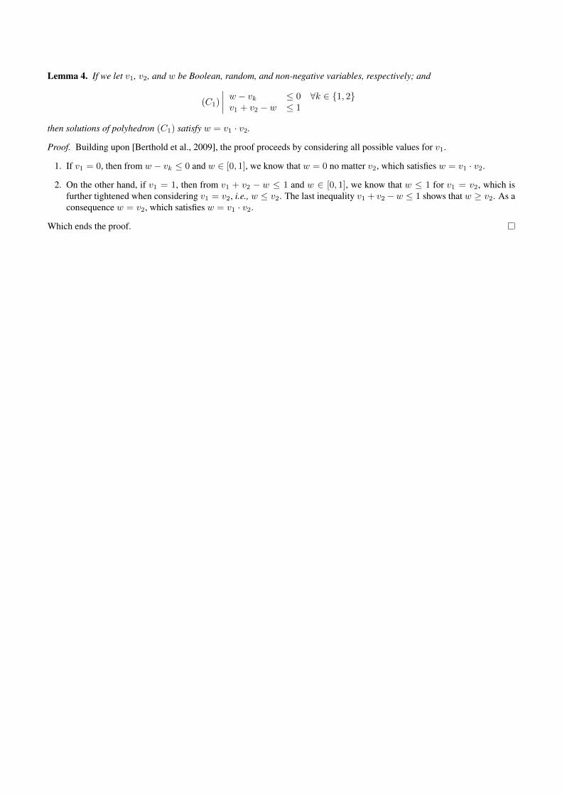
Lemma 4 ([Berthold et al., 2009]). If we let v1, v2, and wbe Boolean, random, and non-negative variables, respec-tively; and
(C1)
∣∣∣∣ w − vk ≤ 0 ∀k ∈ {1, 2}v1 + v2 − w ≤ 1
then solutions of polyhedron (C1) satisfy w = v1 · v2.
The next property shows for the first time how to ex-ploit Lemma 4 to reformulate nonlinear constraints fromn-agent cases into linear ones.
Proposition 1. If we let ζ(x, o1:n, u1:n) be a joint distri-bution and {ai(oi, ui)}i∈N+
≤nbe Boolean variables; and
(Cζ(oi, ui))
∣∣∣∣ Pζ(oi, ui)− ai(oi, ui) ≤ 0Pζ(oi) + ai(oi, ui)− Pζ(oi, ui) ≤ 1
then solutions of polyhedron {Cζ(oi, ui)}i∈N+≤n
satisfy
ζ(x, o1:n, u1:n) = Pζ(x, o1:n)∏ni=1Pζ(ui|oi)
ai(oi, ui) = Pζ(ui|oi).
Proof. The extended occupancy state ζ(x, o, u) can be re-written equivalently as follows:
ζ(x, o, u).= Pζ(x, o1:n)
∏nj=1Pζ(uj |oj)
= Pζ(x, o−i, u−i|oi, ui)Pζ(oi)Pζ(ui|oi) (7)= Pζ(x, o−i, u−i|oi, ui)Pζ(oi, ui) (8)
Since LHS of both (7) and (8) are equal, we have equiva-lently
Pζ(oi, ui) = Pζ(oi)Pζ(ui|oi), ∀i, oi, ui. (9)
Using Lemma 4 along with the fact that {Pζ(ui|oi)} areBoolean variables (and the obvious result that Pζ(oi, ui)−Pζ(oi) ≤ 0), we know that solutions of {Cζ(oi, ui)} alsosatisfy (9). Equality ai(oi, ui) = Pζ(ui|oi) follows di-rectly from Lemma 4. Indeed, if Pζ(oi) = 0, the firstinequality implies ai(oi, ui) = 0(= Pζ(ui|oi)); otherwisePζ(oi) = 0, and Lemma 4 gives us Pζ(oi, ui) = ai(oi, ui)·Pζ(oi) 6= 0, so that ai(oi, ui) = Pζ(oi, ui)/Pζ(oi) =Pζ(ui|oi) using Bayes rule.
We are now poised to present a MILP to solving generaldecentralized stochastic control problems.
Theorem 1. If we let {ai(oi, ui)} and {ζ(x, o, u)} beBoolean and non-negative variables, respectively, then asolution of mixed-integer linear program (P2):
maxa1:n,ζ
Eζ{r(x, u)} s.t. (5) and {Cζ(oi, ui)}i,oi∈Oi,ui∈Ui
is an ε-optimal solution of (P1), where ai is agent i’s policyand ζ denotes the extended occupancy measure.
Proof. From Oliehoek et al. [2008], we know there alwaysexists a deterministic history-dependent decentralized pol-icy that is as good as any randomized history-dependentdecentralized policy. Moreover, as previously discussed,by restricting attention to `-order Markov decentralizedpolicies, the best possible performance in this subclass iswithin ‖r‖∞ · α`/(1− α) of the optimal performance, i.e.,the regret of taking arbitrary decisions from time step ` on-ward. Hence, by searching in the space of deterministicand `-order Markov decentralized policies, i.e., one indi-vidual `-order Markov policy ai for each agent i ∈ N+
≤n,we preserve ability to find an ε-optimal solution of the
original problem Mn under the discounted-reward crite-rion, where ε ≤ ‖r‖∞ · α`/(1− α). Since ai is agenti’s policy and ζ denotes the extended occupancy mea-sure, we know that {ai(oi, ui)} and {ζ(x, o1:n, u1:n)} areBoolean and non-negative variables, respectively. Thus,from Proposition 1, we have that solutions of polyhe-dron {Cζ(oi, ui)}i,oi∈Oi,ui∈Ui satisfy ζ(x, o1:n, u1:n) =s(x, o1:n)
∏ni=1 ai(oi, ui) and s(x, o1:n) are marginal
probabilities Pζ(x, o1:n) and ai(oi, ui) are conditionalprobabilities Pζ(ui|oi) for i ∈ N+
≤n.
This theorem establishes a general MILP to finding an ε-optimal policy in Mn under the discounted-reward crite-rion. We will refer to this problem as the exact MILP. Un-fortunately, the state, action, history spaces for practicalproblems are enormous due to the curse of dimensionality.Consequently, the MILP of interest involves prohibitivelylarge numbers of variables and constraints. (P2) considersless constraints than its nonlinear counterpart (P1), but thesame number of variables. Variables in (P1) are all free,whereas variables {ai(oi, ui)}i∈N+
≤n,oi∈Oi,ui∈Uiin (P2)
are Boolean and remainders {ζ(x, o, u)}x∈X,o∈O,u∈U arefree.
5 Tractable SubclassesIn this section, we present two examples involving themixed-integer linear formulations for subclasses of decen-tralized partially observable Markov decision processes.The intention is to illustrate more concretely how the for-mulation might be achieved and how reasonable choiceslead to near-optimal policies. We shall consider joint-observability and weak-separability assumptions.
5.1 Joint observability assumptionWe first consider a setting where agents collectively ob-serve the true state of the world. This assumption,known as joint observability, arises in many decentralizedMarkov decision processes [Bernstein et al., 2002], e.g.,transition-independent decentralized Markov decision pro-cesses [Becker et al., 2004]. More formally, we say thata system is jointly observable if and only if there exists asurjective function ϕ : Z 7→ X which prescribes the truestate of the world given the current joint observation.
Corollary 1. Under joint observability assumption, ifwe let ai(zi, ui)i∈N+
≤nand ζ(z, u) be Boolean and non-
negative variables, respectively, then:(i) the transition probability from observation z to obser-vation z′ upon taking action u is
puϕ(z, z′).=∑x∈Xδx(ϕ(z))
∑y∈Xp
u(x, y) · qu(y, z′),
where the rewards over observations is given by rϕ(z, u).=∑
x∈X δx(ϕ(z)) · r(x, u); and the initial distribution overobservations is given by νϕ(z)
.=∑x∈X δx(ϕ(z))ν(x);
(ii) the occupancy measures over observations satisfy
s>(I − αP a) .= (1− α)ν>ϕ ; (10)
(iii) a solution of mixed-integer linear program (P3)
maxa1:n,ζ
Eζ{rϕ(z, u)} s.t. (10) and {Cζ(zi, ui)}i,zi∈Zi,ui∈Ui
is also solution of (P2), where ai is agent i’s policy and ζdenotes the extended occupancy measure.
This corollary presents an approximate mixed-integer lin-ear program that can find Markov decentralized policiesunder joint observability. Markov policies, a.k.a. 1-orderMarkov policies, act depending only upon the current ob-servation. This formulation depends on states and historiesonly through the current observations, which results in asignificant reduction in the number of variables and con-straints, i.e., from O(|X||O||U |) in (P2) to O(|Z||U |) in(P3). Interestingly, this formulation finds optimal policiesin transition-independent decentralized Markov decisionprocesses, as deterministic Markov policies were provento be optimal in such a setting [Goldman and Zilberstein,2004].
5.2 Weak separability assumptionNext, we consider the weak separability assumption, whicharises in network-distributed partially observable Markovdecision processes [Nair et al., 2005]. The assumption al-lows us to decouple variables involved in the approximatemixed-integer linear programs into factors, i.e., subsets ofvariables, which make it possible to scale up to large num-ber of agents. The intuition behind this assumption is thatnot all agents interact with one another; often an agent in-teracts only with a small subset of its neighbors, hence itsdecisions may not affect the remainder of its teammates.To take into account the locality of interaction, we makethe following assumptions.
Definition 3. Let E be a set of subsets e of agents. Adecentralized partially observable Markov decision pro-cess (n,X,Z, U, q, p, r, ν) is said to be weakly separableif the following holds: n denotes the number of agents;X
.= X0 × X1 × · · · × Xn; ν is multiplicatively fully
separable, i.e., there exists (νi)i∈N≤n such that ν(x) =∏i∈N≤n
νi(xi), where x = (xi)i∈N≤n ; p is multiplica-tively weakly separable, i.e., there exists (pi)i∈N≤n suchthat puee (xe, ye) = p0(x0, y0)
∏i∈e p
uii (xi, yi), where
xe = (x0, (xi)i∈e) and ue = (ui)i∈e; q is multiplica-tively weakly separable, i.e., there exists (qi)i∈N+
≤nsuch
that quee (ze, ye) =∏i∈e q
uii (zi, yi), where ye = (yi)i∈e,
ze = (zi)i∈e and ue = (ui)i∈e; r is additively weaklyseparable, i.e., there exists (re)e∈E such that r(x, u) =∑e∈E re(xe, ue), for all state and action x, u.
This assumption suggests two agents, i and j, can onlyaffect one another if they share the same subset e, i.e.,i, j ∈ e; otherwise they can choose what to do with noknowledge about what the other sees or plans to do. As aconsequence, the value function in this setting is proven tobe additively weakly separable [Dibangoye et al., 2014a],
i.e., Eζ{r(x, u)} =∑e∈E Eζe{re(x, u)}, where
s>e (I − αP ae).= (1− α)ν>e , (11)
describes the recursion definition of the occupancy mea-sure se extract from the extended occupancy measure ζe.The following exploits this property to define an exactmixed-integer linear program that decouples variables ac-cording to E, resulting in significant dimensionality reduc-tion.
Corollary 2. Let Mn be weakly separable. If we let{ai(oi, ui)}i∈N+
≤n, and {ζe(xe, oe, ue)} be Boolean and
non-negative variables, respectively; then a solution ofmixed-integer linear program (P4)
maxa1:n,ζ
∑e∈EEζe{re(xe, ue)} s.t. (11) and {Cζe(oi, ui)}
is also a network-distributed solution of (P2), where whereai is agent i’s policy and ζe denotes the extended occu-pancy measure for all e.
This mixed-integer linear program exploits the so-calledweak separability assumption that arises under locality ofinteraction. It is worth mentioning that (P4) can find anoptimal policy for network-distributed partially observableMarkov decision processes, assuming reasonable choice ofhistories Oe for each subset of agents e [Dibangoye et al.,2014a].
6 Adaptive Decentralized ControlIn this section, we extend to decentralized partially ob-servable Markov decision processes the probing algorithmoriginally introduced for Markov decision processes. Sim-ilarly to the original algorithm, ours alternates betweenmodel estimation and policy improvement phases foreveror until the training budget is exhausted. The estimatorsof both dynamics {Pτ} and exploration policies {πτ} shallinvolve counting the number of times the algorithm vis-its state-action-state-observation quadruplets (x, u, y, z),state-action pairs (x, u), and states x after τ interactionsbetween the agent and the environment—by an abuse ofnotation we shall use wτ (x, u, y, z), wτ (x, u), wτ (x) tostore these numbers, respectively. It is worth noticing thatsince the model does not depend on histories, maintain-ing history-dependent policies {aτ} is useless, instead itsuffices to maintain state-dependent policies {πτ} corre-sponding to extended occupancy measures {ζτ}.Under standard ergodicity conditions, the model estima-tion phase ensures each state-action pairs is visited in-finitely often, making Pτ = {pu,zτ (x, y)} a consistent es-timator of dynamics after τ interactions: pu,zτ (x, y) =wτ (x, u, y, z)/wτ (x, u), if wτ (x, u) > 0 and chosen arbi-trary otherwise. In other terms, if each state-action pair isvisited infinitely often, then by the strong law of large num-ber, limτ→∞ Pτ = P . To do so, we make use of an explo-ration strategy, namely probe. To better understand the
probing exploration policy, let U(x) = {1, . . . , |U(x)|} bethe set of available actions in state x ∈ X , and σ(x) be thenumber of actions to be experienced in state x ∈ X . Beforea new estimation phase starts, we set σ(x) = |U(x)| for ev-ery state x ∈ X . At each time step of the model estimationphase, if σ(x) > 0, the centralized coordinator executesaction σ(x) in state x and decrements σ(x); otherwise, heor she selects the action which minimizes the difference be-tween the estimated and the optimized exploration policies(updated at the improvement phase), denoted πτ and πτ ,respectively: for any arbitrary x ∈ X and vector of countsσ,
probe(x, σ).=
{σ(x), if σ(x) > 0argminu∈U(x)
{πτ (u|x)− πτ (u|x)}, otherwise.
If the state space forms a single positive recurrent classunder any stationary policy, probe ensures every state-action pair gets visited at least once at each model estima-tion phase, in which case the estimation phase terminates.Otherwise, we shall impose a training budget τmax duringeach model estimation phase. Once the budget is exhaustedthe estimation phase stops—in that case, there is no guar-antee of visiting every state-action pair. Next, the algorithmproceeds to the policy-improvement phase.Each policy-improvement phase starts by computing an ex-tended occupancy measure ζτ for the current estimate dy-namics Pτ using our MILP formulations. Then, it calcu-lates the state-dependent exploration policy as follows:
πτ (u|x) =∑oζτ (x, o, u)/
∑x,oζτ (x, o, u). (12)
Next, it ensures πτ.= {πτ (u|x)} is a consistent estimator
of πτ , where πτ (u|x).= wτ (x, u)/wτ (x), if wτ (x) > 0;
and 0 otherwise. To this end, it explores the state spaceby selecting the action which minimizes the difference be-tween the estimated and the optimized exploration poli-cies, until ‖πτ − πτ‖∞ goes below a certain threshold.It is worth noticing that that this algorithm requires nohyper-parameter tuning. We present the pseudocode of ourprobing algorithm in the supplementary material.
7 ExperimentsThis section empirically demonstrates and validates thescalability of the proposed planning and learning approachw.r.t. the number of agents for α = 0.9. We show that ourplanning and learning approach applies to n-agent Dec-POMDPs where no other MILP formulation does. Werun our experiments on Intel(R) Xeon(R) CPU E5-2623 v33.00GHz.
7.1 ND-POMDPsSetup. We conduct experiments on well-establishedbenchmarks for evaluating n-agent Dec-POMDPs, i.e.network-distributed domains based on the sensor networkapplications [Nair et al., 2005], which range from four tofifteen agents. The reader interested in the description of
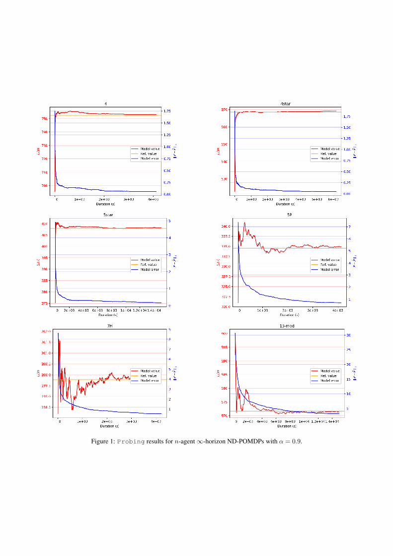
Figure 1: Probing results for n-agent∞-horizon ND-POMDPs with α = 0.9.
Algorithm |a| Time Jα(a; ν)4 domain — |X| = 12, n = 4, |Zi| = 2, and 2 ≤ |Ui| ≤ 3
P4(` = 1) 3× 3 0.37s 752.492P4(` = 2) 5× 5 0.39s 752.492
4-star domain — |X| = 12, n = 4, |Zi| = 2, and 2 ≤ |Ui| ≤ 3P4(` = 1) 3× 3 0.279s 568.642P4(` = 2) 5× 5 0.298s 568.642
5-star domain — |X| = 12, n = 5, |Zi| = 2, and 2 ≤ |Ui| ≤ 3P4(` = 1) 3× 3 0.932s 407.821P4(` = 2) 5× 5 1.241s 407.821
5-P domain — |X| = 12, n = 5, |Zi| = 2, and 2 ≤ |Ui| ≤ 3P4(` = 1) 3× 3 7.12s 334.536P4(` = 2) 5× 5 10.01s 334.536
7-H domain — |X| = 12; n = 7, |Zi| = 2, and 2 ≤ |Ui| ≤ 3P4(` = 1) 3× 3 5.10s 199.773P4(` = 2) 5× 5 7.63s 199.77315-3D domain — |X| = 60; n = 15, |Zi| = 2, and 2 ≤ |Ui| ≤ 4P4(` = 1) 3× 3 1328.48s 409.069P4(` = 2) 5× 5 3002.19s 409.06915-Mod domain — |X| = 16; n = 15, |Zi| = 2, and 2 ≤ |Ui| ≤ 4P4(` = 1) 3× 3 27.1845s 571.642P4(` = 2) 5× 5 59.238s 571.642
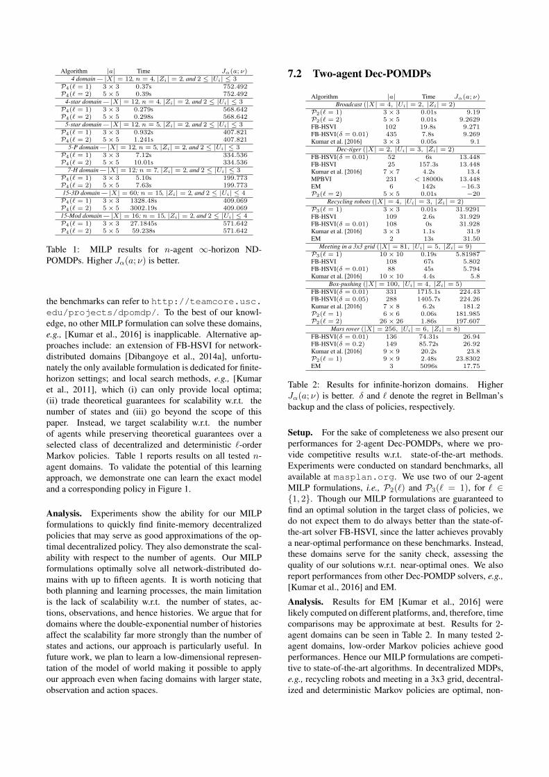
Table 1: MILP results for n-agent ∞-horizon ND-POMDPs. Higher Jα(a; ν) is better.
the benchmarks can refer to http://teamcore.usc.edu/projects/dpomdp/. To the best of our knowl-edge, no other MILP formulation can solve these domains,e.g., [Kumar et al., 2016] is inapplicable. Alternative ap-proaches include: an extension of FB-HSVI for network-distributed domains [Dibangoye et al., 2014a], unfortu-nately the only available formulation is dedicated for finite-horizon settings; and local search methods, e.g., [Kumaret al., 2011], which (i) can only provide local optima;(ii) trade theoretical guarantees for scalability w.r.t. thenumber of states and (iii) go beyond the scope of thispaper. Instead, we target scalability w.r.t. the numberof agents while preserving theoretical guarantees over aselected class of decentralized and deterministic `-orderMarkov policies. Table 1 reports results on all tested n-agent domains. To validate the potential of this learningapproach, we demonstrate one can learn the exact modeland a corresponding policy in Figure 1.
Analysis. Experiments show the ability for our MILPformulations to quickly find finite-memory decentralizedpolicies that may serve as good approximations of the op-timal decentralized policy. They also demonstrate the scal-ability with respect to the number of agents. Our MILPformulations optimally solve all network-distributed do-mains with up to fifteen agents. It is worth noticing thatboth planning and learning processes, the main limitationis the lack of scalability w.r.t. the number of states, ac-tions, observations, and hence histories. We argue that fordomains where the double-exponential number of historiesaffect the scalability far more strongly than the number ofstates and actions, our approach is particularly useful. Infuture work, we plan to learn a low-dimensional represen-tation of the model of world making it possible to applyour approach even when facing domains with larger state,observation and action spaces.
7.2 Two-agent Dec-POMDPs
Algorithm |a| Time Jα(a; ν)Broadcast (|X| = 4, |Ui| = 2, |Zi| = 2)
P2(` = 1) 3× 3 0.01s 9.19P2(` = 2) 5× 5 0.01s 9.2629FB-HSVI 102 19.8s 9.271FB-HSVI(δ = 0.01) 435 7.8s 9.269Kumar et al. [2016] 3× 3 0.05s 9.1
Dec-tiger (|X| = 2, |Ui| = 3, |Zi| = 2)FB-HSVI(δ = 0.01) 52 6s 13.448FB-HSVI 25 157.3s 13.448Kumar et al. [2016] 7× 7 4.2s 13.4MPBVI 231 < 18000s 13.448EM 6 142s −16.3P2(` = 2) 5× 5 0.01s −20
Recycling robots (|X| = 4, |Ui| = 3, |Zi| = 2)P3(` = 1) 3× 3 0.01s 31.9291FB-HSVI 109 2.6s 31.929FB-HSVI(δ = 0.01) 108 0s 31.928Kumar et al. [2016] 3× 3 1.1s 31.9EM 2 13s 31.50
Meeting in a 3x3 grid (|X| = 81, |Ui| = 5, |Zi| = 9)P3(` = 1) 10× 10 0.19s 5.81987FB-HSVI 108 67s 5.802FB-HSVI(δ = 0.01) 88 45s 5.794Kumar et al. [2016] 10× 10 4.4s 5.8
Box-pushing (|X| = 100, |Ui| = 4, |Zi| = 5)FB-HSVI(δ = 0.01) 331 1715.1s 224.43FB-HSVI(δ = 0.05) 288 1405.7s 224.26Kumar et al. [2016] 7× 8 6.2s 181.2P2(` = 1) 6× 6 0.06s 181.985P2(` = 2) 26× 26 1.86s 197.607
Mars rover (|X| = 256, |Ui| = 6, |Zi| = 8)FB-HSVI(δ = 0.01) 136 74.31s 26.94FB-HSVI(δ = 0.2) 149 85.72s 26.92Kumar et al. [2016] 9× 9 20.2s 23.8P2(` = 1) 9× 9 2.48s 23.8302EM 3 5096s 17.75
Table 2: Results for infinite-horizon domains. HigherJα(a; ν) is better. δ and ` denote the regret in Bellman’sbackup and the class of policies, respectively.
Setup. For the sake of completeness we also present ourperformances for 2-agent Dec-POMDPs, where we pro-vide competitive results w.r.t. state-of-the-art methods.Experiments were conducted on standard benchmarks, allavailable at masplan.org. We use two of our 2-agentMILP formulations, i.e., P2(`) and P3(` = 1), for ` ∈{1, 2}. Though our MILP formulations are guaranteed tofind an optimal solution in the target class of policies, wedo not expect them to do always better than the state-of-the-art solver FB-HSVI, since the latter achieves provablya near-optimal performance on these benchmarks. Instead,these domains serve for the sanity check, assessing thequality of our solutions w.r.t. near-optimal ones. We alsoreport performances from other Dec-POMDP solvers, e.g.,[Kumar et al., 2016] and EM.
Analysis. Results for EM [Kumar et al., 2016] werelikely computed on different platforms, and, therefore, timecomparisons may be approximate at best. Results for 2-agent domains can be seen in Table 2. In many tested 2-agent domains, low-order Markov policies achieve goodperformances. Hence our MILP formulations are competi-tive to state-of-the-art algorithms. In decentralized MDPs,e.g., recycling robots and meeting in a 3x3 grid, decentral-ized and deterministic Markov policies are optimal, non-
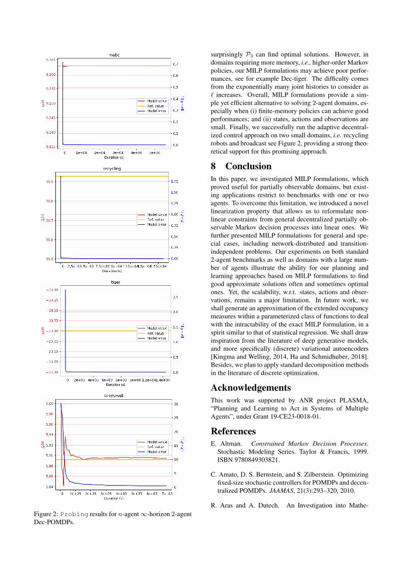
Figure 2: Probing results for n-agent∞-horizon 2-agentDec-POMDPs.
surprisingly P3 can find optimal solutions. However, indomains requiring more memory, i.e., higher-order Markovpolicies, our MILP formulations may achieve poor perfor-mances, see for example Dec-tiger. The difficulty comesfrom the exponentially many joint histories to consider as` increases. Overall, MILP formulations provide a sim-ple yet efficient alternative to solving 2-agent domains, es-pecially when (i) finite-memory policies can achieve goodperformances; and (ii) states, actions and observations aresmall. Finally, we successfully run the adaptive decentral-ized control approach on two small domains, i.e. recyclingrobots and broadcast see Figure 2, providing a strong theo-retical support for this promising approach.
8 ConclusionIn this paper, we investigated MILP formulations, whichproved useful for partially observable domains, but exist-ing applications restrict to benchmarks with one or twoagents. To overcome this limitation, we introduced a novellinearization property that allows us to reformulate non-linear constraints from general decentralized partially ob-servable Markov decision processes into linear ones. Wefurther presented MILP formulations for general and spe-cial cases, including network-distributed and transition-independent problems. Our experiments on both standard2-agent benchmarks as well as domains with a large num-ber of agents illustrate the ability for our planning andlearning approaches based on MILP formulations to findgood approximate solutions often and sometimes optimalones. Yet, the scalability, w.r.t. states, actions and obser-vations, remains a major limitation. In future work, weshall generate an approximation of the extended occupancymeasures within a parameterized class of functions to dealwith the intractability of the exact MILP formulation, in aspirit similar to that of statistical regression. We shall drawinspiration from the literature of deep generative models,and more specifically (discrete) variational autoencoders[Kingma and Welling, 2014, Ha and Schmidhuber, 2018].Besides, we plan to apply standard decomposition methodsin the literature of discrete optimization.
AcknowledgementsThis work was supported by ANR project PLASMA,“Planning and Learning to Act in Systems of MultipleAgents”, under Grant 19-CE23-0018-01.
ReferencesE. Altman. Constrained Markov Decision Processes.
Stochastic Modeling Series. Taylor & Francis, 1999.ISBN 9780849303821.
C. Amato, D. S. Bernstein, and S. Zilberstein. Optimizingfixed-size stochastic controllers for POMDPs and decen-tralized POMDPs. JAAMAS, 21(3):293–320, 2010.
R. Aras and A. Dutech. An Investigation into Mathe-
matical Programming for Finite Horizon DecentralizedPOMDPs. JAIR, 37:329–396, 2010.
R. Becker, S. Zilberstein, V. R. Lesser, and C. V. Goldman.Solving Transition Independent Decentralized MarkovDecision Processes. JAIR, 22:423–455, 2004.
D. S. Bernstein, R. Givan, N. Immerman, and S. Zil-berstein. The Complexity of Decentralized Control ofMarkov Decision Processes. Mathematics of OperationsResearch, 27(4), 2002.
T. Berthold, S. Heinz, and M. E. Pfetsch. Nonlinearpseudo-boolean optimization: relaxation or propaga-tion? Technical Report 09-11, ZIB, Takustr. 7, 14195Berlin, 2009.
J. S. Dibangoye, C. Amato, O. Buffet, and F. Charpillet.Optimally Solving Dec-POMDPs As Continuous-stateMDPs. In IJCAI, pages 90–96, 2013.
J. S. Dibangoye, C. Amato, O. Buffet, and F. Charpillet.Exploiting Separability in Multi-Agent Planning withContinuous-State MDPs. In AAMAS, pages 1281–1288,2014a.
J. S. Dibangoye, C. Amato, O. Buffet, and F. Charpillet.Optimally solving Dec-POMDPs as Continuous-StateMDPs: Theory and Algorithms. Research Report RR-8517, INRIA, 2014b.
C. V. Goldman and S. Zilberstein. Decentralized Controlof Cooperative Systems: Categorization and ComplexityAnalysis. JAIR, 22(1):143–174, 2004. ISSN 1076-9757.
D. Ha and J. Schmidhuber. Recurrent world models fa-cilitate policy evolution. In NeurIPS, pages 2450–2462,2018.
D. P. Kingma and M. Welling. Auto-encoding variationalbayes. stat, 1050:1, 2014.
A. Kumar, S. Zilberstein, and M. Toussaint. Scalable Mul-tiagent Planning Using Probabilistic Inference. In AAAI,pages 2140–2146, 2011.
A. Kumar, S. Zilberstein, and M. Toussaint. ProbabilisticInference Techniques for Scalable Multiagent DecisionMaking. JAIR, 53:223–270, 2015.
A. Kumar, H. Mostafa, and S. Zilberstein. Dual formula-tions for optimizing Dec-POMDP controllers. In ICAPS,pages 202–210, 2016.
H. Mostafa and V. Lesser. Compact mathematical pro-grams for dec-mdps with structured agent interactions.In UAI, pages 523–530, 2011.
R. Nair, P. Varakantham, M. Tambe, and M. Yokoo. Net-worked Distributed POMDPs: A Synthesis of Dis-tributed Constraint Optimization and POMDPs. InAAAI, pages 133–139, 2005.
F. A. Oliehoek. Sufficient Plan-Time Statistics for Decen-tralized POMDPs. In IJCAI, 2013.
F. A. Oliehoek, M. T. J. Spaan, and N. A. Vlassis. Optimaland Approximate Q-value Functions for DecentralizedPOMDPs. JAIR, 32:289–353, 2008.
S. Seuken and S. Zilberstein. Formal models and algo-rithms for decentralized decision making under uncer-tainty. JAAMAS, 17(2):190–250, 2008.
D. Szer, F. Charpillet, and S. Zilberstein. MAA*: AHeuristic Search Algorithm for Solving DecentralizedPOMDPs. In UAI, 2005.
S. Witwicki and E. Durfee. Commitment-driven distributedjoint policy search. In AAMAS, pages 75:1–75:8, 2007.
J. Wu and E. H. Durfee. Mixed-integer linear program-ming for transition-independent decentralized MDPs. InAAMAS, pages 1058–1060, 2006.
A ProofsLemma 1. sα(ν, a) is a probability distribution.
Proof. Let e be a vector of all ones. Then we have
sα(ν, a)>e
.=
((1− α)ν>
∞∑τ=0
ατ (P a)τ
)e
= (1− α)ν>∞∑τ=0
ατe
= (1− α)ν>(1− α)−1e given∞∑τ=0
ατ = (1− α)−1
= ν>e
= 1 ν being a probability distribution
and the claim follows.
Lemma 2. sα(ν, a) is a sufficient statistic for estimating infinite-horizon normalized discounted reward:
Jα(a; ν) = Easα(ν,a){r(x, u)}. (4)
Proof. Let measure ν>(P a)τ be the probability distribution over state-history pairs conditional on initial state distribution νand policy a, after τ decision epochs. Then we have
Jα(a; ν).= (1− α)
∞∑τ=0
ατEaν{r(xτ , uτ )}
= (1− α)∞∑τ=0
ατE{r(xτ , uτ ) | {(xτ , oτ ) ∼ ν>(P a)τ , uτ ∼ a(oτ , ·)}
= (1− α)∞∑τ=0
ατ∑x∈X
∑o∈O
(ν>(P a)τ )(xτ = x, oτ = o)∑u∈U
a(o, u) · r(x, u)
=∑x∈X
∑u∈U
r(x, u)∑o∈O
a(o, u)
((1− α)ν>
∞∑τ=0
ατ (P a)τ
)(xτ = x, oτ = o)
=∑x∈X
∑u∈U
r(x, u)∑o∈O
a(o, u) · sα(ν, a;x, o)
.= Easα(ν,a){r(x, u)}
and the claim follows.
Lemma 3. Occupancy measure sα(ν, a) is the solution of the following linear equation w.r.t. sα(ν, a):
sα(ν, a)>(I − αP a) = (1− α)ν>. (5)
Proof. If we let I be the identity matrix, the following holds:
∞∑τ=0
ατP aν (τ) = ν>∞∑τ=0
ατ (P a)τ = ν>(I − αP a)−1. (13)
Injecting (13) into (3), and re-arranging terms lead to a linear characterization of occupancy measures:
sα(ν, a)>(I − αP a) = (1− α)ν>.
Which ends the proof.
Lemma 4. If we let v1, v2, and w be Boolean, random, and non-negative variables, respectively; and
(C1)
∣∣∣∣ w − vk ≤ 0 ∀k ∈ {1, 2}v1 + v2 − w ≤ 1
then solutions of polyhedron (C1) satisfy w = v1 · v2.
Proof. Building upon [Berthold et al., 2009], the proof proceeds by considering all possible values for v1.
1. If v1 = 0, then from w − vk ≤ 0 and w ∈ [0, 1], we know that w = 0 no matter v2, which satisfies w = v1 · v2.
2. On the other hand, if v1 = 1, then from v1 + v2 − w ≤ 1 and w ∈ [0, 1], we know that w ≤ 1 for v1 = v2, which isfurther tightened when considering v1 = v2, i.e., w ≤ v2. The last inequality v1 + v2 −w ≤ 1 shows that w ≥ v2. As aconsequence w = v2, which satisfies w = v1 · v2.
Which ends the proof.