Multiazimuth coherence

Jie Qi1, Fangyu Li1, and Kurt Marfurt1

ABSTRACT

Since its introduction two decades ago, coherence has beenwidely used to map structural and stratigraphic discontinuitiessuch as faults, cracks, karst collapse features, channels, strati-graphic edges, and unconformities. With the intent to map azimu-thal variations of horizontal stress as well as to improve thesignal-to-noise ratio of unconventional resource plays, wide-/full-azimuth seismic data acquisition has become common. Mi-grating seismic traces into different azimuthal bins costs no morethan migrating them into one bin. If the velocity anisotropy is nottaken into account by the migration algorithm, subtle discontinu-ities and somemajor faults may exhibit lateral shifts, resulting in asmeared image after stacking. Based on these two issues, weevaluate a new way to compute the coherence for azimuthallylimited data volumes. Like multispectral coherence, we modify

the covariance matrix to be the sum of the covariance matrices,each of which belongs to an azimuthally limited volume, and thenwe use the summed covariance matrix to compute the coherentenergy. We validate the effectiveness of our multiazimuth coher-ence by applying it to two seismic surveys acquired over the FortWorth Basin, Texas. Not surprisingly, multiazimuth coherenceexhibits less incoherent noise than coherence computed fromazimuthally limited amplitude volumes. If the data have beenmigrated using an azimuthally variable velocity, multiazimuth co-herence exhibits higher lateral resolution than that computed fromthe stacked data. In contrast, if the data have not been migratedusing an appropriate azimuthally variable velocity model, themisalignment of each image results in a blurring of the multi-azimuth coherence and the coherence computed from the stackeddata. This suggests that our method may serve as a future tool forazimuthal velocity analysis.

INTRODUCTION

Seismic attributes are routinely used to quantify changes in am-plitude, dip, and reflector continuity in seismic amplitude volumes.Coherence is an edge-detection attribute that maps lateral changesin waveforms, which may be due to structural discontinuities, strati-graphic discontinuities, pinchouts, or steeply dipping coherentnoise cutting more gently dipping reflectors. Several generationsof coherence algorithms have been introduced and applied to geo-logic discontinuity detection, such as crosscorrelation (Bahorichand Farmer, 1995), semblance (Marfurt et al., 1998), the eigenstruc-ture method (Gersztenkorn and Marfurt, 1999), the gradient struc-ture tensor (Bakker, 2002), and predictive error filtering (Bednar,1998) algorithms. All those algorithms operate on a spatial windowof neighboring traces (Chopra and Marfurt, 2007).Bahorich and Farmer’s (1995) crosscorrelation algorithm

searches along candidate dips for the highest positive normalized

crosscorrelation coefficient between the pilot trace and the nearesttwo or four neighboring traces in the inline and crossline directionsresulting in values between 0 (incoherent) and 1 (coherent). Marfurtet al.’s (1998) semblance algorithm computes the ratio of the energyof the average trace to the average energy of all the traces in ananalysis window. To improve the semblance for fault detection,some authors (Hale, 2013; Wu and Hale, 2016; Wu et al., 2016)apply fault-oriented smoothing to the numerator and denominatorof the semblance ratio to compute a fault-likelihood value. Gersz-tenkorn and Marfurt’s (1999) eigenstructure-based coherence algo-rithm first computes a covariance matrix from a window of tracesegments oriented along a structural dip. In this algorithm, coher-ence is computed as the ratio of the first eigenvalue to the sum of allthe eigenvalues of the covariance matrix. The energy-ratio coher-ence algorithm (Chopra and Marfurt, 2007) also uses a covariancematrix, from windowed analytic traces (the original data and its Hil-bert transform), and estimates the coherent component of the data

Manuscript received by the Editor 30 March 2017; revised manuscript received 19 May 2017; published ahead of production 13 July 2017; published online29 August 2017.

1University of Oklahoma, ConocoPhillips School of Geology and Geophysics, Norman, Oklahoma, USA. E-mail: jie.qi@ou.edu; fangyu.li@ou.edu;kmarfurt@ou.edu.

© 2017 Society of Exploration Geophysicists. All rights reserved.

O83

GEOPHYSICS, VOL. 82, NO. 6 (NOVEMBER-DECEMBER 2017); P. O83–O89, 6 FIGS.10.1190/GEO2017-0196.1

Dow

nloa

ded

10/2

4/17

to 6

8.97

.115

.26.

Red

istr

ibut

ion

subj

ect t

o SE

G li

cens

e or

cop

yrig

ht; s

ee T

erm

s of

Use

at h

ttp://

libra

ry.s

eg.o

rg/

using a Karhunen-Loève (KL) filter. Like semblance, energy-ratiocoherence is the ratio of the energy of the coherent (KL filtered)analytic traces to that of the original analytic traces. Bakker (2002)computes a version of coherence called “chaos” by computingeigenvalues of the gradient structure tensor. The 3 × 3 gradientstructure tensor is computed by crosscorrelating derivatives of theseismic amplitude in the x-, y-, and z-directions. The first eigen-value represents the energy of the data variability (or gradient)perpendicular to the reflector dip. If the data can be represented bya constant-amplitude planar event, the chaos is equal to −1.0. Incontrast, if the data are totally random, the chaos is equal to þ1.0.Similarly, Wu (2017) computes directional structure-tensor-basedcoherence for detecting seismic faults and channels. Closely relatedto coherence is Luo et al.’s. (1996) generalized Hilbert transformedge-detection algorithm, a long-wavelength version of Luo et al.’s(2003) Sobel filter discontinuity algorithm. Kington (2015) com-pares different coherence algorithms and exhibits the trade-offsamong different implementations.Picking discontinuities on vertical slices through the seismic am-

plitude volume is still the most common means to map faults onseismic data. However, coherence not only accelerates this processbut also delineates channel edges, carbonate build-ups, slumps,

collapse features, and angular unconformities (Sullivan et al.,2006; Schuelke, 2011; Qi et al., 2014). Coherence can also be usedas an input seismic texture in multiattribute seismic facies analysis(Qi et al., 2016).With the focus on shale resource plays, wide-azimuth surveys are

commonly acquired to orient horizontal wells perpendicular to themaximum horizontal stress direction for optimum completion.Wide-azimuth surveys provide greater leverage against coherentnoise such as ground roll and interbed multiples. Wide-azimuth,higher fold surveys also are amenable to modern surface-consistentstatics solutions. The axes of azimuthal anisotropy are commonlyaligned parallel and perpendicular with open fractures or micro-cracks. Finally, wide-azimuth surveys provide the data necessaryfor azimuthal anisotropy analysis. Several authors have computedattributes from azimuthally limited volumes with only moderate re-sults. Barnes (2000) proposes a smoothing technique to reducenoise and spikes from instantaneous attributes computed from post-stack data. Perez et al. (1999) compute spectral components fromdifferent azimuths and find it to be an indicator of anisotropy. Cho-pra and Marfurt (2007) find coherence computed from such lower-fold data to exhibit higher lateral resolution but also to be noisy.Al-Dossary et al. (2004) attempt perhaps the first interazimuthcoherence algorithm but find it provides greater sensitivity to dataquality than to geology.A related problem is the computation of coherence from spec-

trally limited data volumes. Li and Lu (2014) and Li et al. (2015)compute coherence from different spectral components and coren-der them using a red, green, and blue (RGB) color model. Sui et al.(2015) add covariance matrices computed from a suite of spectralmagnitude components, obtaining a coherence image superior tothat of the original broadband data. Marfurt (2017) expands on thisidea, adds coherence matrices computed from analytic spectralcomponents (the spectral voices and their Hilbert transforms) alongthe structural dip, and obtains improved suppression of randomnoise and enhancement of small faults and karst collapse features.In this paper, we build on this last piece of work, but we now

generalize it to summing covariance matrices computed from a suiteof azimuthally limited, rather than frequency-limited, volumes. Webegin our paper with a review of the energy-ratio coherence algo-rithm. We then show the improved lateral resolution but reducedsignal-to-noise ratio (S/N) of coherence images generated from azi-muthally limited seismic data. Next, we show how the multiazimuthcoherence computation provides superior results when applied to adata volume that has been properly migrated using an azimuthallyvarying velocity model. Finally, we apply the multiazimuth coher-ence algorithm to a data volume that has not been properly correctedfor azimuthal anisotropy. We conclude with a summary of ourobservations and a short list of recommendations.

METHOD

Coherence is an edge-detection attribute that measures lateralchanges in the seismic waveform and amplitude. The multiazimuthcoherence algorithm is based on an energy-ratio coherence algorithm,which computes the ratio of coherent energy of seismic trace and totalenergy of seismic trace (Appendix A). Figure 1 shows 2K þ 1 ¼ 7

sample vectors of length M ¼ 5, where one sample vector is con-structed from interpolation of samples from each of five traces. Weuse the semblance technique to compute inline and crossline structuraldip components of one analysis point from the poststack image. Then,

Figure 1. Cartoon of an analysis window with five traces and sevensamples. (a) Five input traces (U1 − U5) extracted from a poststackseismic amplitude volume through the structural dip and (b) com-puted coherent traces (UKL1 − UKL5) from five input traces. We usethe semblance technique to compute inline and crossline structuraldip components of each analysis point from the poststack image.Then, we build the analysis window by extracting its neighboringsamples along the inline and crossline dips. The computations ofcoherent traces are introduced in Appendix A. Note that the waveletamplitude of the three leftmost traces is about two times larger thanthat of the two rightmost traces.

O84 Qi et al.

Dow

nloa

ded

10/2

4/17

to 6

8.97

.115

.26.

Red

istr

ibut

ion

subj

ect t

o SE

G li

cens

e or

cop

yrig

ht; s

ee T

erm

s of

Use

at h

ttp://

libra

ry.s

eg.o

rg/

Figure 2. Time slices at t ¼ 0.74 s through azimuthally limited migrated seismic amplitude (Amp) volumes: (a) 165°–15°, (b) 15°–45°,(c) 45°–75°, (d) 75°–105°, (e) 105°–135°, and (f) 135°–165°. Note the azimuthal variations and that although the S/N of each azimuthal sectoris low, one can identify the faults and karst features.

Figure 3. Time slices at t ¼ 0.74 s through coherence (Coh) volumes computed from the azimuthally limited data shown in Figure 2: (a) 165°–15°,(b) 15°–45°, (c) 45°–75°, (d) 75°–105°, (e) 105°–135°, and (f) 135°–165°. Although one can identify faults and karst collapse features, the images arequite noisy.

Multiazimuth coherence O85

Dow

nloa

ded

10/2

4/17

to 6

8.97

.115

.26.

Red

istr

ibut

ion

subj

ect t

o SE

G li

cens

e or

cop

yrig

ht; s

ee T

erm

s of

Use

at h

ttp://

libra

ry.s

eg.o

rg/

we build the analysis window by extracting its neighboring samplesthrough inline and crossline dips. The principal component (Karhu-nen-Loève) filtered traces are shown in Figure 1b. More details ofthe energy-ratio coherence algorithm are shown in Appendix A.Migrating seismic traces into bins depending on the source-

receiver orientation provides azimuthally limited seismic amplitudevolumes. Using a migration isotropic velocity may give rise toimaging misalignments in high azimuthally anisotropic reservoirs.Stacking those seismic gathers along offset domains results in azi-muthally limited seismic amplitude volumes. Coherence computedfrom the poststack volume that stacking all azimuthally limited seis-mic amplitude volumes exhibits fewer geologic details and lowerlateral resolution of migrated seismic images than coherence com-puted from azimuthally limited seismic amplitude volumes (Chopraand Marfurt, 2007). Stacking these azimuthally limited amplitudevolumes can suppress random noise. We will show that coherencecomputed from the full stack is generally less noisy than that com-puted from azimuthally limited volumes.

Multiazimuth coherence

We generalize the concept of energy-ratio coherence by summingJ covariance matrices CðφjÞ computed from each of the J azimu-thally sectored data volumes:

Cmulti−φ ¼XJ

j¼1

CðφjÞ: (1)

The summed covariance matrix is of the same M ×M size as theoriginal single-azimuth covariance matrix, but it is now composedof J times as many sample vectors. As the conventional covariancematrix, the multiazimuth covariance matrix is a symmetric positivedefinite matrix. Eigendecomposition of the multiazimuth covari-ance matrix is a nonlinear process, such that the first eigenvectorof the summed covariance matrix is not a linear combination ofthe first eigenvectors computed for the azimuthally limited covari-ance matrices, in which case the resulting coherence would be theaverage of the azimuthally limited coherence computations.Geologic details in each azimuthally seismic image are trans-

ferred into sample vectors. Summing the sample vectors providesa means of summing geologic anomalies into the multiazimuthcovariance matrix, such as stacking up azimuthally limited coher-ence. This nonlinear eigendecomposition of the multiazimuthcovariance matrix has advantages in suppressing random noise thatwould help deal with random noise in azimuthally limited seismicvolumes. To lessen the computation cost, azimuths are commonlybinned into six 30° or eight 22.5° sectors, although finer binning iscommon in large processing shops.

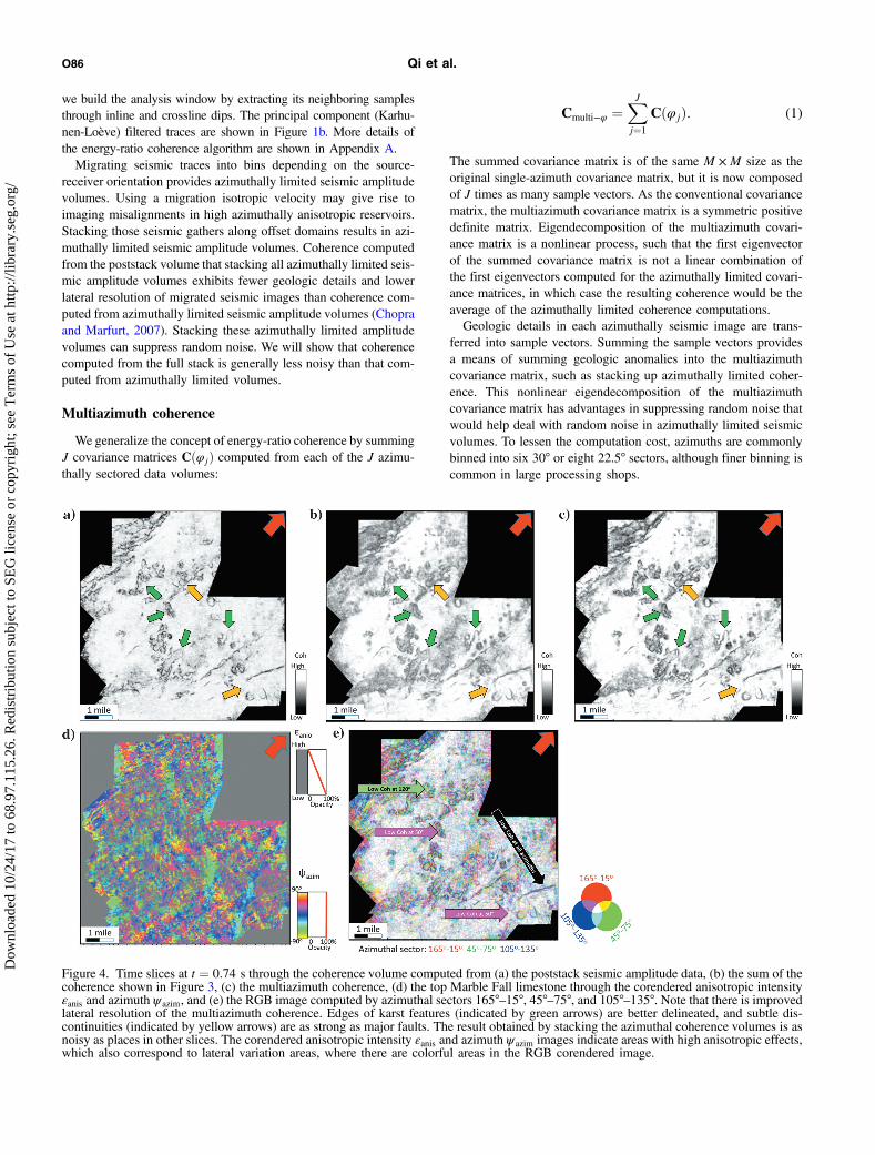
Figure 4. Time slices at t ¼ 0.74 s through the coherence volume computed from (a) the poststack seismic amplitude data, (b) the sum of thecoherence shown in Figure 3, (c) the multiazimuth coherence, (d) the top Marble Fall limestone through the corendered anisotropic intensityεanis and azimuth ψ azim, and (e) the RGB image computed by azimuthal sectors 165°–15°, 45°–75°, and 105°–135°. Note that there is improvedlateral resolution of the multiazimuth coherence. Edges of karst features (indicated by green arrows) are better delineated, and subtle dis-continuities (indicated by yellow arrows) are as strong as major faults. The result obtained by stacking the azimuthal coherence volumes is asnoisy as places in other slices. The corendered anisotropic intensity εanis and azimuth ψ azim images indicate areas with high anisotropic effects,which also correspond to lateral variation areas, where there are colorful areas in the RGB corendered image.

O86 Qi et al.

Dow

nloa

ded

10/2

4/17

to 6

8.97

.115

.26.

Red

istr

ibut

ion

subj

ect t

o SE

G li

cens

e or

cop

yrig

ht; s

ee T

erm

s of

Use

at h

ttp://

libra

ry.s

eg.o

rg/

Application

Our two examples are from the Fort Worth Basin, Texas. Survey Awas acquired in 2006 using 16 live receiver lines forming awide-azimuth survey with a nominal 16.7 × 16.7 m (55 × 55 ft)common-depth point (CDP) bin size. The data were preprocessedand binned into six azimuths, preserving the amplitude fidelity at eachstep before prestack time migration (Roende et al., 2008). A 3 trace ×3 trace × 7 sample (inline axis × crossline axis × vertical axis)analysis window is used to compute coherence. In general, smallerwindows are better if the S/N allows it. Vertical windows larger thanthe dominant period smear stratigraphic edges. Figure 2 shows timeslices at t ¼ 0.74 s through the six different azimuthally limited seis-mic amplitude volumes. Figure 3 shows time slices through the sixcorresponding coherence volumes. Because the S/N of each azimu-thal sector seismic amplitude is low, the S/N of the resulting coher-ence images is also low. The differences between the six azimuthallylimited coherence images include the shape and size of karst features(indicated by green arrows), the continuity of subtle faults (indicatedby yellow arrows), and the level of incoherent noise. As recognizedby Perez and Marfurt (2008), faults are best delineated by the azi-muths perpendicular to them (e.g., Figure 3a at 0° versus Figure 3cat 60°).Stacking the six seismic amplitude volumes and then computing

coherence (the conventional analysis workflow) gives the resultshown in Figure 4a. This image shows an increased S/N but aslightly lower lateral resolution than the azimuthally limited coher-ence time slices shown in Figure 3. Figure 4b shows the result ofstacking the six images shown in Figure 3. Theresolution on Figure 4b is lower than that of Fig-ure 4a; however, edges of the karst features ap-pear more pronounced than on the traditionalcoherence computation. Figure 4c shows themultiazimuth coherence result computed usingthe covariance matrix described by equation 1.Note that multiazimuth coherence displays thehigher spatial resolution than either traditionalcoherence or stacked azimuthal coherence, espe-cially in areas with high anisotropy (indicated inFigure 4d). Karst features (indicated by green ar-rows) exhibit highly incoherent anomalies,whereas subtle faults (indicated by yellow ar-rows) appear as strong as the major faults. Multi-azimuth coherence not only preserves most of thediscontinuities seen in each of the azimuthallylimited coherence volumes in Figure 3 but alsosuppresses incoherent noise. Figure 4e showsthe RGB corendered azimuthally limited coher-ence 165°–15° (red), 45°–75° (green), and 105°–135° (blue). If the three input azimuthal coher-ence volumes were perfectly aligned, the coher-ent part of the corendered RGB image would bewhite and aligned faults would be black. In Fig-ure 4e, most areas are well-aligned and are indi-cated by the white color; however, faults andkarst collapse features are less well-aligned, andthey are mapped by colors other than black. Ma-genta arrows indicate low coherence at 45°–75°,and the green arrow indicates low coherence at105°–135°, whereas the black arrow indicates

low coherence for all three input volumes. Note that areas with highanisotropy in Figure 4d give rise to colorful or misaligned anoma-lies in Figure 4e.Survey B is also from the Fort Worth Basin, Texas. The data

were prestack time migrated into eight azimuthal sectors at 22.5°intervals. Figure 5 shows time slices at t ¼ 1.36 s through fourof the coherence volumes 0°–22.5°, 45°–67.5°, 90°–112.5°, and135°–157.5°. These data were migrated using an isotropic velocitymodel, such that anisotropy gives rise to lateral shifts (indicated byyellow arrows) in the coherence anomalies. Zhang et al. (2014,2015) and Verma et al. (2016) apply a prestack structure-orientedfilter to suppress coherent noise, processing, and migration artifacts.Perez and Marfurt (2008) apply a spatial crosscorrelation techniqueto the coherence slices to measure lateral shifts of discontinuitiesand then correct them using a data warping algorithm. Figure 6aillustrates a time slice through coherence computed from thestacked seismic amplitude volume. Note the S/N in Figure 6a ishigher than that in Figure 5 because random noise is suppressedafter stacking azimuthally limited seismic amplitude volumes.However, despite being noisy, the images in Figure 5 exhibit ahigher lateral resolution than Figure 6a. Lateral shifts (indicatedby yellow arrows) of discontinuities observed from different azimu-thally limited coherence volumes have been smeared by stacking.In general, applying isotropic velocity to either area with aniso-tropic effects due to microcracks opening perpendicular to the mini-mum horizontal stress direction in this survey gives rise toazimuthal variations of discontinuities. Guo et al. (2016) compare

Figure 5. Time slices at t ¼ 1.36 s through the coherence volume computed from theazimuthal sector (a) 0°–22.5°, (b) 45°–67.5°, (c) 90°–112.5°, and (d) 135°–157.5° in thesecond data set. Note that there are significant differences between each azimuthal co-herence. The lateral shifts of the discontinuities are indicated by the yellow arrows.

Multiazimuth coherence O87

Dow

nloa

ded

10/2

4/17

to 6

8.97

.115

.26.

Red

istr

ibut

ion

subj

ect t

o SE

G li

cens

e or

cop

yrig

ht; s

ee T

erm

s of

Use

at h

ttp://

libra

ry.s

eg.o

rg/

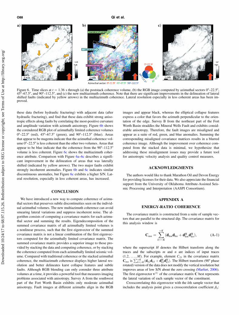
these data (before hydraulic fracturing) with adjacent data (afterhydraulic fracturing), and find that these data exhibit strong aniso-tropic effects along faults by correlating the most-positive curvatureand amplitude variation with azimuth anisotropy. Figure 6b showsthe corendered RGB plot of azimuthally limited coherence volumes0°–22.5° (red), 45°–67.5° (green), and 90°–112.5° (blue). Areasthat appear to be magenta indicate that the azimuthal coherence vol-ume 0°–22.5° is less coherent than the other two volumes. Areas thatappear to be blue indicate that the coherence from the 90°–112.5°volume is less coherent. Figure 6c shows the multiazimuth coher-ence attribute. Comparison with Figure 6a–6c describes a signifi-cant improvement in the delineation of areas that was laterallyshifted (indicated by yellow arrows). The two major faults exhibitstrongly incoherent anomalies. Figure 6b and 6c indicates similardiscontinuous anomalies, but Figure 6c exhibits a higher S/N. Lat-eral resolution, especially in less coherent areas, has increased.

CONCLUSION

We have introduced a new way to compute coherence of azimu-thal sectors that preserves subtle discontinuities seen on the individ-ual azimuthal volumes. The new multiazimuth coherence can avoidsmearing lateral variations and suppress incoherent noise. The al-gorithm consists of computing a covariance matrix for each azimu-thal sector and summing the results. Eigendecomposition of thesummed covariance matrix of all azimuthally limited volumes isa nonlinear process, such that the first eigenvector of the summedcovariance matrix is not a linear combination of the first eigenvec-tors computed for the azimuthally limited covariance matrix. Thesummed covariance matrix provides a superior image to those pro-vided by stacking the data and computing coherence, or by stackingthe coherence computed from each azimuthally limited seismic vol-ume. Compared with traditional coherence or the stacked azimuthalcoherence, the multiazimuth coherence displays higher lateral res-olution and better delineates karst collapse features and subtlefaults. Although RGB blending can only corender three attributevolumes at a time, it provides a powerful tool that measures imagingproblems associated with anisotropy. Survey A from the southwestpart of the Fort Worth Basin exhibits only moderate azimuthalanisotropy. Fault images at different azimuths align in the RGB

images and appear black, whereas the elliptical collapse featuresexpress a color that favors the azimuth perpendicular to the orien-tation of the edge. Survey B from the northeast part of the FortWorth Basin straddles the Mineral Wells Fault and exhibits consid-erable anisotropy. Therefore, the fault images are misaligned andappear as a suite of red, green, and blue anomalies. Summing thecorresponding misaligned covariance matrices results in a blurredcoherence image. Although the improvement over coherence com-puted from the stacked data is minimal, we hypothesize thataddressing these misalignment issues may provide a future toolfor anisotropic velocity analysis and quality control measures.

ACKNOWLEDGMENTS

The authors would like to thank Marathon Oil and Devon Energyfor providing licenses for their data. We also appreciate the financialsupport from the University of Oklahoma Attribute-Assisted Seis-mic Processing and Interpretation (AASPI Consortium).

APPENDIX A

ENERGY-RATIO COHERENCE

The covariance matrix is constructed from a suite of sample vec-tors that are parallel to the structural dip. The covariance matrix forthis analysis window is

Cmn ¼XþK

k¼−Kðdkmdkn þ dHkmd

HknÞ; (A-1)

where the superscript H denotes the Hilbert transform along thetraces and the subscripts m and n are indices of input traces(1;2; : : : ;M). For example, element C23 in the covariance matrixCmn is

PþKk¼−Kðdk2dk3 þ dHk2d

Hk3Þ. The Hilbert transform (90° phase

rotated) version of the data does not modify the vertical resolution butimproves areas of low S/N about the zero crossing (Marfurt, 2006).The first eigenvector vð1Þ of the covariance matrix C best representsthe lateral variation of each sample vector of the constituent.Crosscorrelating this eigenvector with the kth sample vector that

includes the analysis point gives a crosscorrelation coefficient βk:

Figure 6. Time slices at t ¼ 1.36 s through (a) the poststack coherence volume, (b) the RGB image computed by azimuthal sectors 0°–22.5°,45°–67.5°, and 90°–112.5°, and (c) the new multiazimuth coherence. Note that there are significant improvements in the delineation of lateralshifted faults (indicated by yellow arrows) in the multiazimuth coherence. Lateral resolution especially in less coherent areas has been im-proved.

O88 Qi et al.

Dow

nloa

ded

10/2

4/17

to 6

8.97

.115

.26.

Red

istr

ibut

ion

subj

ect t

o SE

G li

cens

e or

cop

yrig

ht; s

ee T

erm

s of

Use

at h

ttp://

libra

ry.s

eg.o

rg/

βk ¼XM

m¼1

dkmvð1Þm : (A-2)

The principal component (Karhunen-Loève) filtered data within theanalysis window are then

d KLkm ¼ βkv

ð1Þm : (A-3)

Note that in Figure 1, the wavelet amplitude of the three leftmosttraces is about two times larger than that of the two rightmost traces.After filtering, this proportion is preserved.Energy-ratio coherence computes the ratio of the coherent energy

and the total energy in an analysis window:

CER ¼ Ecoh

Etot þ ε2; (A-4)

where the coherent energy Ecoh (the energy of the KL-filtered data)is

Ecoh ¼XþK

k¼−K

XM

m¼1

½ðdKLkmÞ2 þ ðdHKLkm Þ2�; (A-5)

whereas the total energy Etot of unfiltered data in the analysis win-dow is

Etot ¼XþK

k¼−K

XM

m¼1

½ðdkmÞ2 þ ðdHkmÞ2�; (A-6)

and where a small positive value ε prevents division by zero.

REFERENCES

Al-Dossary, S., Y. Simon, and K. J. Marfurt, 2004, Interazimuth coherenceattributes for fracture detection: 74th Annual International Meeting, SEG,Expanded Abstracts, 183–186.

Bahorich, M. S., and S. L. Farmer, 1995, 3-D seismic discontinuity for faultsand stratigraphic features: The Leading Edge, 14, 1053–1058, doi: 10.1190/1.1437077.

Bakker, P., 2002, Image structure analysis for seismic interpretation: Ph.D.thesis, Delft University of Technology.

Barnes, A. E., 2000, Weighted average seismic attributes: Geophysics, 65,275–285, doi: 10.1190/1.1444718.

Bednar, J. B., 1998, Least-squares dip and coherency attributes: The LeadingEdge, 17, 775–778, doi: 10.1190/1.1438051.

Chopra, S., and K. J. Marfurt, 2007, Seismic attributes for prospect identi-fication and reservoir characterization: SEG.

Gersztenkorn, A., and K. J. Marfurt, 1999, Eigenstructure based coherencecomputations as an aid to 3D structural and stratigraphic mapping: Geo-physics, 64, 1468–1479, doi: 10.1190/1.1444651.

Guo, S., S. Verma, Q. Wang, B. Zhang, and K. J. Marfurt, 2016, Vectorcorrelation of amplitude variation with azimuth and curvature in a

post-hydraulic-fracture Barnett Shale survey: Interpretation, 4, no. 1,SB23–SB35, doi: 10.1190/INT-2015-0103.1.

Hale, D., 2013, Methods to compute fault images, extract fault surfaces, andestimate fault throws from 3D seismic images: Geophysics, 78, no. 2,O33–O43, doi: 10.1190/geo2012-0331.1.

Kington, J., 2015, Semblance, coherence, and other discontinuity attributes:The Leading Edge, 34, 1510–1512, doi: 10.1190/tle34121510.1.

Li, F., and W. Lu, 2014, Coherence attribute at different spectral scales:Interpretation, 2, no. 1, SA99–SA106, doi: 10.1190/INT-2013-0089.1.

Li, F., J. Qi, and K. J. Marfurt, 2015, Attribute mapping of variable thicknessincised valley-fill systems: The Leading Edge, 34, 48–52, doi: 10.1190/tle34010048.1.

Luo, Y., S. al-Dossary, M. Marhoon, and M. Alfaraj, 2003, GeneralizedHilbert transform and its application in geophysics: The Leading Edge,22, 198–202, doi: 10.1190/1.1564522.

Luo, Y., W. G. Higgs, and W. S. Kowalik, 1996, Edge detection and strati-graphic analysis using 3D seismic data: 66th Annual International Meet-ing, SEG, Expanded Abstracts, 324–327.

Marfurt, K. J., 2006, Robust estimates of 3D reflector dip and azimuth: Geo-physics, 71, no. 4, P29–P40, doi: 10.1190/1.2213049.

Marfurt, K. J., 2017, Interpretational value of multispectral coherence: 79thAnnual International Conference and Exhibition, EAGE, Extended Ab-stracts, doi: 10.3997/2214-4609.201700528.

Marfurt, K. J., R. L. Kirlin, S. H. Farmer, and M. S. Bahorich, 1998,3D seismic attributes using a running window semblance-based algo-rithm: Geophysics, 63, 1150–1165, doi: 10.1190/1.1444415.

Perez, G., and K. J. Marfurt, 2008, Warping prestack imaged data to improvestack quality and resolution: Geophysics, 73, no. 2, P1–P7, doi: 10.1190/1.2829986.

Perez, M., R. Gibson, and M. N. Toksöz, 1999, Detection of fracture ori-entation using azimuthal variation of P-wave AVO response: Geophysics,64, 1253–1265, doi: 10.1190/1.1444632.

Qi, J., B. Zhang, H. Zhou, and K. J. Marfurt, 2014, Attribute expressionof fault-controlled karst — Fort Worth Basin, TX: Interpretation, 2,no. 3, SF91–SF110, doi: 10.1190/INT-2013-0188.1.

Qi, J., T. Lin, T. Zhao, F. Li, and K. J. Marfurt, 2016, Semisupervised multi-attribute seismic facies analysis: Interpretation, 4, no. 1, SB91–SB106,doi: 10.1190/INT-2015-0098.1.

Roende, H., C. Meeder, J. Allen, S. Peterson, and D. Eubanks, 2008,Estimating subsurface stress direction and intensity from subsurfacefull-azimuth land data: 78th Annual International Meeting, SEG, Ex-panded Abstracts, 217–220.

Schuelke, J. S., 2011, Overview of seismic attribute analysis in shale play:Attributes: New views on seismic imaging: Their use in exploration andproduction: Presented at the 31st Annual GCSSEPM Foundation Bob F.Perkins Research Conference.

Sui, J.-K., X. Zheng, and Y. Li, 2015, A seismic coherency method usingspectral attributes: Applied Geophysics, 12, 353–361, doi: 10.1007/s11770-015-0501-5.

Sullivan, E. C., K. J. Marfurt, A. Lacazette, and M. Ammerman, 2006, Ap-plication of new seismic attributes to collapse chimneys in the Fort Worthbasin: Geophysics, 71, no. 4, B111–B119, doi: 10.1190/1.2216189.

Verma, S., S. Guo, and K. J. Marfurt, 2016, Data conditioning of legacyseismic using migration-driven 5D interpolation: Interpretation, 4,no. 2, SG31–SG40, doi: 10.1190/INT-2015-0157.1.

Wu, X., 2017, Directional structure-tensor-based coherence to detect seismicfaults and channels: Geophysics, 82, no. 2, A13–A17, doi: 10.1190/geo2016-0473.1.

Wu, X., and D. Hale, 2016, 3D seismic image processing for faults: Geo-physics, 81, no. 2, IM1–IM11, doi: 10.1190/geo2015-0380.1.

Wu, X., S. Luo, and D. Hale, 2016, Moving faults while unfaulting 3Dseismic images: Geophysics, 81, no. 2, IM25–IM33, doi: 10.1190/geo2015-0381.1.

Zhang, B., D. Chang, T. Lin, and K. J. Marfurt, 2015, Improving the qualityof prestack inversion by prestack data conditioning: Interpretation, 3,no. 1, T5–T12, doi: 10.1190/INT-2014-0124.1.

Zhang, B., T. Zhao, J. Qi, and K. J. Marfurt, 2014, Horizon-based semiau-tomated nonhyperbolic velocity analysis: Geophysics, 79, no. 6,U15–U23, doi: 10.1190/geo2014-0112.1.

Multiazimuth coherence O89

Dow

nloa

ded

10/2

4/17

to 6

8.97

.115

.26.

Red

istr

ibut

ion

subj

ect t

o SE

G li

cens

e or

cop

yrig

ht; s

ee T

erm

s of

Use

at h

ttp://

libra

ry.s

eg.o

rg/