multicopter design optimization and validation · various components such as battery pack, motor...

Modeling, Identification and Control, Vol. 36, No. 2, 2015, pp. 67–79, ISSN 1890–1328

Multicopter Design Optimization and Validation

Øyvind Magnussen Morten Ottestad Geir Hovland

University of Agder, Faculty of Engineering and Science, Department of Engineering Sciences, Jon Lilletuns veg9, 4879 Grimstad, Norway

Abstract

This paper presents a method for optimizing the design of a multicopter unmanned aerial vehicle (UAV,also called multirotor or drone). In practice a set of datasheets is available to the designer for thevarious components such as battery pack, motor and propellers. The designer can not normally designthe parameters of the actuator system freely, but is constrained to pick components based on availabledatasheets. The mixed-integer programming approach is well suited to design optimization in such caseswhen only a discrete set of components is available. The paper also includes an experimental section wherethe simulated dynamic responses of optimized designs are compared against the experimental results. Thepaper demonstrates that mixed-integer programming is well suited to design optimization of multicopterUAVs and that the modeling assumptions match well with the experimental validation.

Keywords: Multicopter, multirotor, drone, UAV, mathematical modeling, design optimization, experi-mental validation.

Nomenclature

ω Speed: [rad/s]

ρ Density of air

Bi,Ah, Bi,V Battery i Ah and voltage

Cp Power coefficient

Ct Thrust coefficient

Di Diameter of propeller i

F, Freq Propeller thrust

g Gravity constant

im, τm Motor current and torque

J Total inertia

Jm,i Inertia of motor i

Jp,i Inertia of propeller i

Lf (D,Na) Length of frame as function of diameterand number of actuators

mL Mass of payload

mb,i Mass of battery i

mm,i Mass of motor i

mp,i Mass of propeller i

n Speed: Revolutions per second

Na Number of actuators

Pb,i, Pm,i, Pp,i Price of battery, motor, propeller i

Ra,Ke,Kt Motor constants

T Actuator torque

Vi, Vm Supply and motor voltages

W Power

doi:10.4173/mic.2015.2.1 c© 2015 Norwegian Society of Automatic Control

http://dx.doi.org/10.4173/mic.2015.2.1

Modeling, Identification and Control

1 Introduction

The interest in multicopters (also called multirotors ordrones) has increased significantly in recent years, bothin academic research and in commercial applications.One example is the Prime Air multicopter by Amazon,see Fig. 1 and Amazon (2015). Other examples are themulticopters designed and developed to demonstrateacrobatic abilities, see for example Hehn and D’Andrea(2014) and the references therein. Despite the largenumber of published works, very little is published ondesign optimization of multicopters given an intendedapplication and desired performance specifications.

In Magnussen et al. (2014) a concept for design opti-mization of a multicopter based on mixed-integer pro-gramming was presented. In the current paper thesame concept is described in more detail giving all thenecessary information to allow a design engineer to re-peat the design procedure. In normal practice, a set ofdatasheets of components such as battery pack, motorsand propellers is available to the designer. Variablessuch as thrust per propeller or motor torque can notbe designed freely, but must be chosen from a fixed setof available datasheets. The mixed-integer program-ming framework solves optimization problems that fallwithin this category. Certain variables are constrainedto be discrete (for example a Boolean variable indi-cating selection of a particular component representedby a datasheet) while others are continuous variables(for example total weight and flight time). As demon-strated in the paper, the mixed-integer linear program-ming framework also allows for approximation of non-linear functions. A nonlinear function is approximatedby a set of discrete regions of the y-axis, each rep-resented by a linear function. The accuracy of theapproximation can be adjusted by changing the totalnumber of linearized regions.

Numerical methods for nonlinear optimization nor-mally suffer from drawbacks such as long computa-tion times and the fact that the methods can endup in undesirable sub-optimal local minima. Exam-ples are Newton-Raphson gradient search methods andevolutionary-based search methods, such as the Com-plex method, see for example Whitney (1969) andTyapin and Hovland (2009) where the optimizationalgorithm took several hours to converge towards anacceptable but sub-optimal solution. A linear pro-gram (LP) on the other hand, using the interior pointmethod, can be solved in polynomial time, see Kar-markar (1984). The solution of an LP with a largenumber of variables can be found quickly using com-mercial solvers such as IBM CPLEX, see IBM (2015).The solution of a mixed-integer linear program (MILP)is built on an LP solver and techniques such as branch-and-bound. The optimization solver formulated in this

Figure 1: Example of multirotor UAV design by Ama-zon for transport and delivery of parcels.

way can handle nonlinear function approximations anddiscrete design variables and returns a repeatable so-lution in relatively short time compared to an itera-tive nonlinear search algorithm where the solution canvary from run to run, depending on the initial condi-tions. It should be noted, however, that mixed-integeroptimization problems are NP-hard, see for exampleClausen (1999).

The paper also contains a section presenting experi-mental validation of the performance of the multicopteractuators. Both the actuator rise-time constants andthe total flight time used in the design optimizationprocedure are compared with the same parameters es-timated from real measurements using the various com-ponents available to the designer. The validation com-pares the performance of four propellers and three mo-tors against the simulation model in three different testcases: I) Longest possible flight time, no payload, II)Longest possible flying time, 1.5kg payload and III)Fastest possible motor response, no payload. For thethree test cases, optimized solutions were calculatedfor multicopters with 4, 6 and 8 actuators, giving atotal of 9 potentially different designs. The resultsdemonstrate that the simulation model matches wellwith the experiments. The experimental validation in-creases the reliability of the optimization results.

The paper is organized as follows: in Section 2 adynamic model of a multicopter actuator is presented.Section 3 gives a detailed description of the design op-timization procedure. Section 4 presents results fromthe experimental validation based on three differenttest cases. Discussion and conclusions are presentedin Section 5.

68

Magnussen, Ottestad and Hovland, “Multicopter Design Optimization and Validation”

2 Modeling

A Simulink model of the multicopter actuator is shownin Fig. 2. The model generates the simulated thrustresponse for the 9 different test cases used in this paper(test cases I, II and III with 4, 6 and 8 actuators). Thepropeller thrusts from the simulation model are latercompared with experiments (force measurements usinga load cell mounted underneath the actuator). Thepropeller thrust is calculated from eq. (1):

F = Ct · ρ · n2 ·D4 (1)

where Ct is the thrust coefficient, ρ is the density of air,n is the rotor speed (rev/sec) and D is the propellerdiameter. The actuator power W and torque T arecalculated from eqs. (2)-(3):

W = Cp · ρ · n3 ·D5 (2)

T =W

ω(3)

where Cp is the power coefficient and w = 2πn is therotor speed (rad/sec). The motor controller and actu-ator dynamics are given by the equations below:

Vm = Vi −Keω (4)

im =VmRa

(5)

τm = Kt · im (6)

dω

dt=

1

J(τm − T ) (7)

where J is the total inertia, Vm, im, τm are the motorvoltage, current and torque, Ke, Kt and Ra are motorparameters and Vi is the supply voltage from the mo-tor controller. Mechanical friction is not included inthe dynamic model in eq. (7), since this information isdifficult to obtain from the manufacturer’s datasheets.Eqs. (1)-(7) are implemented in the Simulink model inFig. 2.

By combining eqs. (2)-(7) and using the fact that forDC motors the motor torque and back emf constantsare equal, that is, Kt = Ke, the following transfer func-tion can be defined:

ω

Vi(s) =

Kt(JRa

K2t +DωRa

)s+ 1

(8)

where Dω = Tω =

ρCpn3D5

ω2 . Assuming constant pa-rameters in eq. (8), the time-constant would be tr =

JRa

K2t +DωRa

. Since Dω is a function of the propeller

speed, this time-constant is an estimation.

3 Design Optimization

A quadratic program is defined as follows:

min xTQx + gTx (9)

subject to : Ax ≤ b (10)

where x ∈ Rn is the state vector to be solved, Q ∈Rn×n is a positive semi-definite penalty matrix, g ∈ Rnis a penalty vector, A ∈ Rm×n is the constraint ma-trix while b ∈ Rm is the constraint vector. When thepenalty matrix Q = 0, eqs. (9)-(10) reduce to a linearprogram. When some elements xi where i ∈ [1, · · · , n]are constrained to be integer variables, eqs. (9)-(10)are called mixed integer quadratic program (MIQP) or,when Q = 0, mixed integer linear program (MILP).

By constraining the integer variables further to ac-cept only Boolean values (0 or 1), logical constraintscan be incorporated and linked with the continuousvariables in the optimization problem. The followingrules 1 and 4 are taken from Bemporad and Morari(1999) and Mignone (2002). Rules 19a and 19b aremodified compared to Mignone (2002) (δ = 0 insteadof δ = 1). In the rule definitions below the followingnotation is used:

m = minx∈X

f(x)

M = maxx∈X

f(x)

ε denotes a small, real, positive constant,

typically the machine precision.

It should be noted that equality constraints of the typeax = b must be converted to two inequality constraintsax ≤ b and −ax ≤ −b to satisfy eq. (10). However,the solver used (CPLEX) allows specification of bothequality and inequality constraints.

Product of Boolean variable and function ofcontinuous variables.

z = δ · f(x)

or

IF [δ == 1] THEN z = f(x)

ELSE z = 0

is equivalent to

−Mδ + z ≤ 0

mδ − z ≤ 0

−mδ + z ≤ f(x)−mMδ − z ≤ −f(x) +M

Rule 1: Product of δ and f(x)

69


Figure 2: Simulink implementation of multirotor actuator dynamics.

Product of several Boolean variables and func-tion of continuous variables.

z =

(n∧i=1

δi

)· f(x)

or

IF

[(n∧i=1

δi

)== 1

]THEN z = f(x)

ELSE z = 0

is equivalent to

z + M

(n∑i=1

δi

)≤ f(x) + nM

z ≤ f(x) + M

−z − m

(n∑i=1

δi

)≤ −f(x)− nm

−z ≤ −f(x)− mz + mδ1 ≤ 0

...

z + mδn ≤ 0

−z − Mδ1 ≤ 0...

−z − Mδn ≤ 0

where M = max(0,−m), m = min(0,−M).

Rule 4: Product of several δ’s and f(x)

The scalar y ≥ 0 equals the nonlinear functiong(·) of the scalar x ∈ [0, xmax]. The set z ap-proximates g(x) by using a set of straight linesegments a ∈ a1, · · · , aN, k ∈ k1, · · · , kN.Only one of the Boolean variables in the setδ ∈ δ1, · · · , δN is true and specifies whichelement in z ∈ z1, · · · , zN is used. M =max(g(x)). The nonlinear function approxi-mation builds on rules 1, 19a and 19b in theequations below:

z1 = δ1(a1x+ k1)

...

zN = δN (aNx+ kN )

[z1 ≤ 0] → [δ1 = 0][z1 ≥

M · 1N

]→ [δ1 = 0]

...[zN ≤

M · (N − 1)

N

]→ [δN = 0]

[zN ≥M ] → [δN = 0]N∑i=1

δi = 1

y =

N∑i=1

zi

Nonlinear positive function: y = g(x)

70


Implication.

[f(x) ≤ fL]→ [δ = 0]

is equivalent to

Mδ ≤ f(x)− fL +M + ε

Rule 19a: Implication of f(x) ≤ fL

Implication.

[f(x) ≥ fU ]→ [δ = 0]

is equivalent to

Mδ ≤ −f(x) + fU +M − ε

Rule 19b: Implication of f(x) ≥ fU

x

y

g(x)

M

12

13

14

z1 = 12(a1x+k1)

z2 = 13(a2x+k2)

z3 = 14(a3x+k3)

M2 3

M1 3

0

Figure 3: Illustration of mixed-integer linear approxi-mation of a nonlinear positive function g(x)with three regions (δ12, δ13 and δ14).

Fig. 3 illustrates how a nonlinear function can beapproximated using a combination of discrete and con-tinuous variables. In this example three regions δ12,δ13 and δ14 are chosen to approximate the nonlinearfunction g(x). The δ’s are chosen to represent an equalspacing on the y-axis in the figure. In each region rep-resented by δi a linear approximation zi = δi(aix+ ki)is used.

The objective function gTx in eq. (9) can be de-fined as shown in Table 1 depending on the applica-tion’s requirement specifications. For payload transferand package delivery, for example, the longest possi-

Criterion Objective functionMin. Time-constant gTx = x16Min. Power gTx = x17Min. Price gTx = x3Max. Flight-time gTx = x21Min. Inertia Roll gTx = x13Min. Inertia Pitch gTx = x14

Table 1: Different candidate objective functions to beminimized/maximized depending on the re-quirement specifications.

Variables Descriptionδ1 · · · δ4 Propeller 1-4 selectionδ5 · · · δ7 Motor 1-3 selectionδ8 · · · δ11 Battery 1-4 selectionδ12 · · · δi1 Used to calculate n3

δi1+1 · · · δi2 Used to calculate inertia (roll)δi2+1 · · · δi3 Used to calculate inertia (pitch)

Table 2: Boolean decision variables. If δ = 1, then thecorresponding component/region is selected.If δ = 0, the component/region is not selected.

ble flight time or smallest possible power consumptionmay be desirable objectives. For acrobatics, on theother hand, the designer may instead want to selectthe solution giving the smallest possible time-constantor smallest possible roll and pitch inertias.

For the multirotor design optimization, the Booleandecision variables δi are defined as shown in Table 2and the continuous variables xi are defined as shownin Table 3. The complete mixed-integer state vector xintroduced in eq. (9) is defined as follows:

x = [δ1 · · · δi3 , x1 · · ·xj12 ]T

(11)

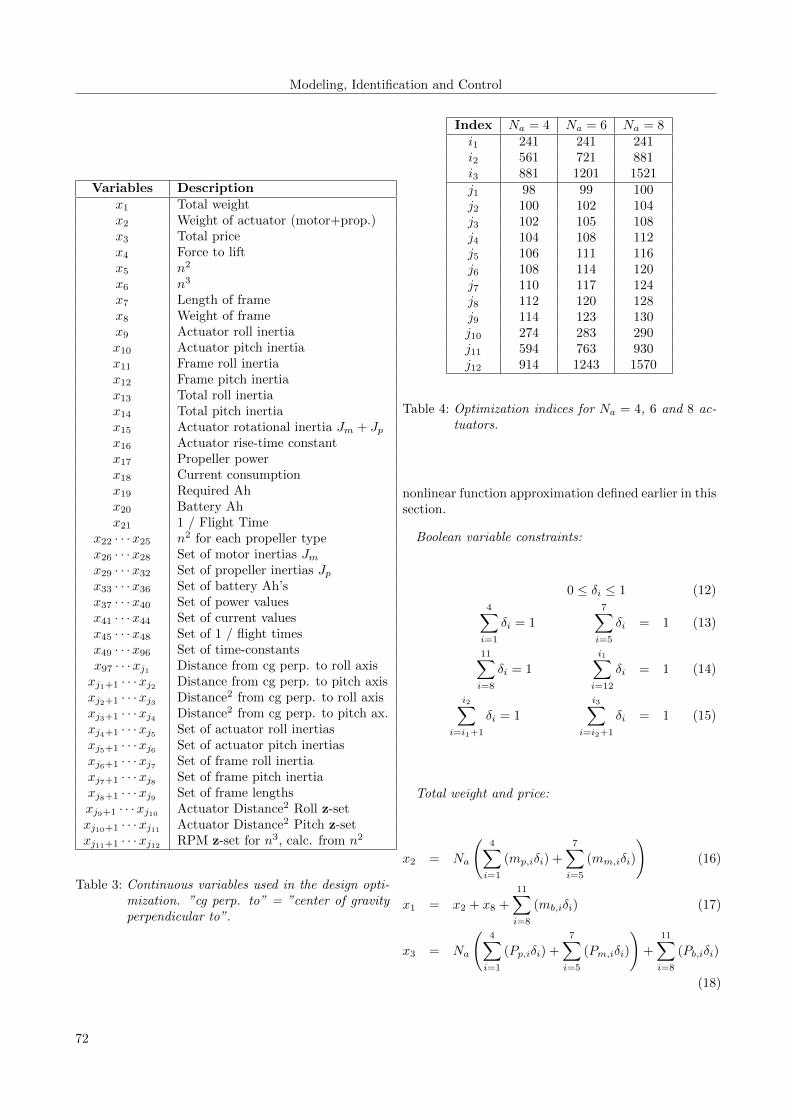
The indices i and j of discrete and continuous variablesare summarized in Table 4. Three different MILPs arecreated. One with the number of actuators constrainedto Na = 4, one with Na = 6 and one with Na = 8.The total number of discrete and continuous variablesvaries between the three programs and is equal to 1795,2444 and 3091, respectively. To avoid multiplication ofseveral free variables in the constraints, it was decidedto create three separate MILPs rather than creatingone optimization program with Na as a free variable.To find the optimal solution, the three MILPs are runseparately and the solution with the lowest objectivefunction value is chosen.

In the following, the complete set of constraints usedin the multicopter design optimization is listed. Theconstraints make use of the rules 1, 4, 19a, 19b and the

71


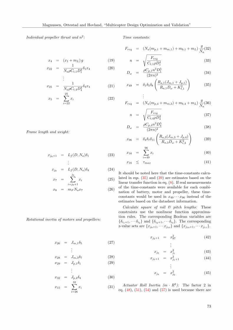
Variables Descriptionx1 Total weightx2 Weight of actuator (motor+prop.)x3 Total pricex4 Force to liftx5 n2

x6 n3

x7 Length of framex8 Weight of framex9 Actuator roll inertiax10 Actuator pitch inertiax11 Frame roll inertiax12 Frame pitch inertiax13 Total roll inertiax14 Total pitch inertiax15 Actuator rotational inertia Jm + Jpx16 Actuator rise-time constantx17 Propeller powerx18 Current consumptionx19 Required Ahx20 Battery Ahx21 1 / Flight Time

x22 · · ·x25 n2 for each propeller typex26 · · ·x28 Set of motor inertias Jmx29 · · ·x32 Set of propeller inertias Jpx33 · · ·x36 Set of battery Ah’sx37 · · ·x40 Set of power valuesx41 · · ·x44 Set of current valuesx45 · · ·x48 Set of 1 / flight timesx49 · · ·x96 Set of time-constantsx97 · · ·xj1 Distance from cg perp. to roll axisxj1+1 · · ·xj2 Distance from cg perp. to pitch axisxj2+1 · · ·xj3 Distance2 from cg perp. to roll axisxj3+1 · · ·xj4 Distance2 from cg perp. to pitch ax.xj4+1 · · ·xj5 Set of actuator roll inertiasxj5+1 · · ·xj6 Set of actuator pitch inertiasxj6+1 · · ·xj7 Set of frame roll inertiaxj7+1 · · ·xj8 Set of frame pitch inertiaxj8+1 · · ·xj9 Set of frame lengthsxj9+1 · · ·xj10 Actuator Distance2 Roll z-setxj10+1 · · ·xj11 Actuator Distance2 Pitch z-setxj11+1 · · ·xj12 RPM z-set for n3, calc. from n2

Table 3: Continuous variables used in the design opti-mization. ”cg perp. to” = ”center of gravityperpendicular to”.

Index Na = 4 Na = 6 Na = 8i1 241 241 241i2 561 721 881i3 881 1201 1521j1 98 99 100j2 100 102 104j3 102 105 108j4 104 108 112j5 106 111 116j6 108 114 120j7 110 117 124j8 112 120 128j9 114 123 130j10 274 283 290j11 594 763 930j12 914 1243 1570

Table 4: Optimization indices for Na = 4, 6 and 8 ac-tuators.

nonlinear function approximation defined earlier in thissection.

Boolean variable constraints:

0 ≤ δi ≤ 1 (12)4∑i=1

δi = 1

7∑i=5

δi = 1 (13)

11∑i=8

δi = 1

i1∑i=12

δi = 1 (14)

i2∑i=i1+1

δi = 1

i3∑i=i2+1

δi = 1 (15)

Total weight and price:

x2 = Na

(4∑i=1

(mp,iδi) +

7∑i=5

(mm,iδi)

)(16)

x1 = x2 + x8 +

11∑i=8

(mb,iδi) (17)

x3 = Na

(4∑i=1

(Pp,iδi) +

7∑i=5

(Pm,iδi)

)+

11∑i=8

(Pb,iδi)

(18)

72


Individual propeller thrust and n2:

x4 = (x1 +mL) g (19)

x22 =1

NaρCt,1D41

δ1x4 (20)

...

x25 =1

NaρCt,4D44

δ4x4 (21)

x5 =

25∑i=22

xi (22)

Frame length and weight:

xj8+1 = Lf (D,Na)δ1 (23)

...

xj9 = Lf (D,Na)δ4 (24)

x7 =

j9∑i=j8+1

xi (25)

x8 = mFNax7 (26)

Rotational inertia of motors and propellers:

x26 = Jm,1δ5 (27)

...

x28 = Jm,3δ7 (28)

x29 = Jp,1δ1 (29)

...

x32 = Jp,4δ4 (30)

x15 =

32∑i=26

xi (31)

Time constants:

Freq = (Na(mp,1 +mm,1) +mb,1 +mL)g

Na(32)

n =

√Freq

Ct,1ρD41

(33)

Dω =ρCp,1n

3D51

(2πn)2(34)

x49 = δ1δ5δ8

(Ra,1(Jm,1 + Jp,1)

Ra,1Dω +K2t,1

)(35)

...

Freq = (Na(mp,4 +mm,3) +mb,4 +mL)g

Na(36)

n =

√Freq

Ct,4ρD44

(37)

Dω =ρCp,4n

3D54

(2πn)2(38)

x96 = δ4δ7δ11

(Ra,3(Jm,3 + Jp,4)

Ra,3Dω +K2t,3

)(39)

x16 =

96∑i=49

xi (40)

x16 ≤ τmax (41)

It should be noted here that the time-constants calcu-lated in eqs. (35) and (39) are estimates based on thelinear transfer function in eq. (8). If real measurementsof the time-constants were available for each combi-nation of battery, motor and propeller, these time-constants would be used in x49 · · ·x96 instead of theestimates based on the datasheet information.

Calculate square of roll & pitch lengths: Theseconstraints use the nonlinear function approxima-tion rules. The corresponding Boolean variables areδi1+1, · · · δi2 and δi2+1, · · · δi3. The correspondingz-value sets are xj9+1, · · ·xj10 and xj10+1, · · ·xj11.

xj2+1 = x297 (42)

...

xj3 = x2j1 (43)

xj3+1 = x2j1+1 (44)

...

xj4 = x2j2 (45)

Actuator Roll Inertia (m · R2): The factor 2 ineq. (48), (51), (54) and (57) is used because there are

73


two actuators per frame arm.

xj4+1 = δ1δ5(mp,1 +mm,1)xj2+1 (46)

...

xj5 = δ4δ7(mp,4 +mm,3)xj3 (47)

x9 = 2

j5∑i=j4+1

xi (48)

Actuator Pitch Inertia (m ·R2):

xj5+1 = δ1δ5(mp,1 +mm,1)xj3+1 (49)

...

xj6 = δ4δ7(mp,4 +mm,3)xj4 (50)

x10 = 2

j6∑i=j5+1

xi (51)

Frame Roll Inertia:

xj6+1 =1

3Lf (D1, Na)mF δ1xj2+1 (52)

...

xj7 =1

3Lf (D4, Na)mF δ4xj3 (53)

x11 = 2

j7∑i=j6+1

xi (54)

Frame Pitch Inertia:

xj7+1 = Lf (D1, Na)mF δ1xj3+1 (55)

...

xj8 = Lf (D4, Na)mF δ4xj4 (56)

x12 = 2

j8∑i=j7+1

xi (57)

Total Roll & Pitch Inertias:

x13 = x9 + x11 (58)

x14 = x10 + x12 (59)

Calculation of n3: This constraint uses the nonlin-ear function approximation rules. The correspondingBoolean variables are δ12, · · · δi1. The correspondingz-value set is xj11+1, · · ·xj12.

x6 = x1.55 (60)

Propeller Power:

x37 = CpρD51δ1x6 (61)

...

x40 = CpρD54δ4x6 (62)

x17 =

40∑i=37

xi (63)

Battery Ah:

x33 = B1,Ahδ8 (64)

...

x36 = B4,Ahδ11 (65)

x20 =

36∑i=33

xi (66)

Current Consumption:

x41 =NaB1,V

δ8x17 (67)

...

x44 =NaB4,V

δ11x17 (68)

x18 =

44∑i=41

xi (69)

Calculate Ah:

x19 =

(TF60

)x18 (70)

x20 = x19 (71)

Calculate the Inverse of Flight Time = A / Ah:

x45 =x18B1,Ah

δ8 (72)

...

x48 =x18B4,Ah

δ11 (73)

x21 =

48∑i=45

xi (74)

4 Experimental Results

The purpose of the experiments presented in this sec-tion is to validate the models and assumptions used inthe mixed-integer optimization presented in section 3.The experimental setup is shown in Fig. 4. The valida-tion presented in this paper has chosen both the 63%rise time of the actuator thrust as well as the total

74


flight time as the parameters to compare against thesimulation model in Fig. 2. The rise times are mea-sured directly from step responses in thrust, while thetotal flight time is estimated via the measured currentwhen the step responses have reached steady-state.

Figure 4: Experimental setup for validation. A: Digi-tal/analog IO card, B: Load cell amplifier, C:Current sensor, D: Battery pack, E: Motorcontroller, F: Propeller, G: Motor, H: Loadcell.

Three different optimization test cases were studied,as summarized below:

• I: Longest possible flying time, no payload

• II: Longest possible flying time, 1.5kg payload

• III: Fastest possible motor response, no payload

The design optimization was constrained to use ei-ther 4, 6 or 8 actuators in the multicopter. Sec-tion 4.1 contains a summary of the different compo-nents (datasheets) available for the design optimiza-tion. The experimental results for each test case aresummarized in sections 4.2, 4.3 and 4.4.

4.1 Summary of Datasheets

The available datasheets are summarized in Table 5, 6and 7. In total three motors (see Fig. 5), four propellers(see Fig. 6) and four batteries were available (the sameas in the design optimization procedure in section 3,Table 2). Since all the batteries have a supply voltageof 11.1V and the experiments focused on validation ofthe 63% rise-time constant and flight time estimatedvia the measured current, the same battery could beused in all the tests, see Fig. 7. The selection of bat-tery in the experiments did not have an impact on theestimated time-constants and total flight time.

Figure 5: Three different motors used in the design op-timization and validation tests.

Figure 6: Four different propellers used in the designoptimization and validation tests.

Figure 7: Battery used in the design validation tests.

75


Motor [#] 1 2 3Model 4108-380KV Turnigy 4108-480KV Turnigy 4108-600KV TurnigyKt,i 380 480 600Ra,i (Ω) 0.222 0.148 0.123mm,i (g) 111 111 111imax,i (A) 17 22 26Pmax,i (W) 360 380 400Dm,i (m) 0.047 0.047 0.047Sl,i (m) 0.012 0.012 0.012Sw,i (m) 0.004 0.004 0.004ρm,i (kg/m3) 6800 6800 6800Pm,i ($) 31.36 31.36 31.36

Table 5: Datasheets: Motors. mm,i is the motor weight, Dm,i is the motor diameter, Sl,i,Sw,i are the shaftlength and width, ρm,i is the material density of the motor and Pm,i is the motor price.

Battery [#] 1 2 3 4mb,i (g) 309 618 1236 308Bi,Ah (mAh) 4000 8000 16000 3300Bi,V (V) 11.1 11.1 11.1 11.1Bi,imax (A) 100 200 400 105Pb,i ($) 25.5 51.0 102.0 26.7

Table 6: Datasheets: Batteries. mb is the weight of the battery, while Pb is the price.

4.2 Test Case I

In this test case the design was optimized for thelongest possible flying time and no payload. As seenin Table 8, propeller 4 was chosen when the design wasconstrained to use 4 and 8 actuators, while propeller 3was chosen with 6 actuators. Motor 3 was chosen with4 and 6 actuators, while motor 2 was chosen with 8 ac-tuators. Battery 3 was chosen regardless of the numberof actuators being 4, 6 or 8. Battery 3 has the high-est capacity (16000 mAh), but also the highest weight.The selection of the battery with the highest capacityis not obvious. The solution with 4 actuators has boththe longest flight time and the lowest price, so it is theprefered design in Test Case I.

Fig. 8 illustrates the experimental results from TestCase I. The black curves show the simulated thrust re-sponse when using the Simulink model in Fig. 2 witheither 4, 6 or 8 actuators. The red curves show themeasured thrust response under acceleration, while thegreen curves show the measured curves under deceler-ation. Note that the green curves are inverted aboutthe steady-state value for easier comparison with theacceleration and the simulated response. The circlesin the figure represent the values at the 63% rise time.The experimental results confirm that a linear modelassumption is appropriate for the multicopter actuator,consisting of battery pack, controller, motor and pro-peller as shown in Fig. 4. Tables 11 and 12 summarize

Propeller [#] 1 2 3 4mp,i (g) 12 14 18 25Dp,i (m) 0.254 0.2794 0.3048 0.3556Ct,i (m) 4.7 4.7 4.7 4.7Cp,i (m) 0.1222 0.1156 0.1146 0.1027pi (deg) 10 11 12 14Pp,i($) 4.7 5.0 5.6 7.8

Table 7: Datasheets: Propellers. mp,i is the weight of the propeller, pi is the pitch angle of the blade and Pp,i isthe propeller price.

76


0 0.1 0.2 0.3 0.4 0.5 0.6 0.7 0.8 0.9 12

2.5

3

3.5

4

4.5

5

5.5

6

Time (sec)

Thr

ust R

espo

nse

(N)

Figure 8: Thrust response per propeller, Test Case I.Top: 4 Actuators, Middle: 6 Actuators, Bot-tom: 8 Actuators. Blue: Input, Red: Accel-eration, Green: Deceleration, Black: Simula-tion model. The circles represent the thrustat the 63% rise time.

the three different rise times (simulation, acceleration,deceleration). For Test Case I the simulated rise timesare slightly faster than the measured values, rangingfrom 30 to 42ms faster.

Number of Actuators 4 6 8Propeller chosen [#] 4 3 4Motor chosen [#] 3 3 2Battery chosen [#] 3 3 3Time constant (ms) 161 165 134Flight time (min) 62.5 60.0 55.5Price 227.4 290.2 352.9

Table 8: Optimization Results: Test Case I.

4.3 Test Case II

In Test Case II the design was optimized for the longestpossible flying time with a 1.5kg payload. As seen inTable 9, propeller 4 and battery 3 were chosen regard-less of the number of actuators being 4,6 or 8. Motor 3was chosen when the design was constrained to 4 and6 actuators, while motor 1 was chosen with 8 actua-tors. The solution with 8 actuators has the longestflight time. However, the price with 8 actuators is sig-nificantly higher than the price for the solutions with4 and 6 actuators.


Table 9: Optimization Results: Test Case II.

0 0.1 0.2 0.3 0.4 0.5 0.6 0.7 0.8 0.9 13

4

5

6

7

8

9

10

11

Time (sec)

Thr

ust R

espo

nse

(N)

Figure 9: Thrust response per propeller, Test Case II.Top: 4 Actuators, Middle: 6 Actuators, Bot-tom: 8 Actuators. Blue: Input, Red: Accel-eration, Green: Deceleration, Black: Simula-tion model. The circles represent the thrustat the 63% rise time.

Fig. 9 illustrates the experimental results from TestCase II. The results for Test Case II are better thanfor Test Case I. Tables 11 and 12 summarize the threedifferent rise times (simulation, acceleration, deceler-ation). For Test Case II the simulated rise times areslightly faster than the measured values, ranging from10 to 15ms faster. Overall, the match between the sim-ulation model and the experiments is good.

4.4 Test Case III

In Test Case III the design was optimized for the fastestpossible motor response and no payload. As seen in Ta-ble 10 propeller 1, motor 1 and battery 1 were chosenregardless of the number of actuators being 4,6 or 8.Since the time-constant (39ms) is the same for 4, 6and 8 actuators, the natural choice is to use the solu-tion with 4 actuators since the flight time is the highest

77


0 0.1 0.2 0.3 0.4 0.5 0.6 0.7 0.8 0.9 1

1.4

1.6

1.8

2

2.2

2.4

2.6

2.8

Time (sec)

Thr

ust R

espo

nse

(N)

Figure 10: Thrust response per propeller, Test CaseIII. Top: 4 Actuators, Middle: 6 Actuators,Bottom: 8 Actuators. Blue: Input, Red:Acceleration, Green: Deceleration, Black:Simulation model. The circles represent thethrust at the 63% rise time.

and the price is the lowest for this choice. Fig. 10 illus-


Table 10: Optimization Results: Test Case III.

trates the experimental results from Test Case III. Theresults for Test Case III are similar to Test Case II. Ta-bles 11 and 12 summarize the three different rise times(simulation, acceleration, deceleration). For Test CaseIII the simulated rise times differ from the measuredvalues by -21ms to +8ms.

Table 13 shows the differences between the time-constants found from the experiments and the esti-mates based on the transfer function in eq. (8) andalso used in the optimization, eqs. (35), (39). The re-sults are satisfactory with differences in the range -41to +25ms. One error source is the time-constant as-sumption made in eq. (8) for a linear system.

The actual flight times can be estimated by dividingthe battery capacity (Ah) by the measured current (A)when the step-responses have reached steady-state and

Test Ta,4 Td,4 Ta,6 Td,6 Ta,8 Td,8I 172 200 118 130 147 167II 146 129 156 146 123 133III 52 72 48 58 43 48

Table 11: Measured rise times (63%, in ms) for the dif-ferent test cases and number of propellers.Ta is for acceleration, Td is for deceleration.

Test T4 ∆T4 T6 ∆T6 T8 ∆T8I 144 -42 92 -32 127 -30II 128 -10 136 -15 114 -14III 41 -21 41 -12 53 8

Table 12: Simulated rise times (63%, in ms) for thedifferent test cases and number of propellers.Ti is the rise time with i propellers. ∆Ti isthe time difference between Ti and the aver-age of Ta,i and Td,i.

by the number of actuators (Na). Table 14 shows theestimated flight times vs. the (inverted) flight timescalculated in eqs. (72)-(74). The standard deviationbetween measured and estimated flight times in Ta-ble 14 is 12.8%. Note that the battery voltage as statedin the datasheets is 11.1V, while the voltage when thebattery is fully charged is more than 12V. In addi-tion, the battery is not capable of keeping the voltagehigher than 11.1V when discharged. Hence, both theestimated flight times and the ones found from experi-ments in Table 14 probably overstate the actual flighttimes slightly.

5 Conclusions

This paper has presented an optimization frameworkfor multirotors based on mixed-integer programming.The framework allows for efficient selection of optimal

Test T4 ∆T4 T6 ∆T6 T8 ∆T8I 186 25 124 -41 157 23II 138 -12 151 -5 128 -5III 62 23 53 14 46 7

Table 13: Time-constants found from experiments(mean value of Ta,i and Td,i in Table 11) forthe different test cases and number of pro-pellers. ∆Ti is the time difference (in ms)between Ti and the time-constant estimatesbased on eq. (8).

78


Test Te,4 To,4 Te,6 To,6 Te,8 To,8I 66.6 62.5 57.5 60.0 62.0 55.5II 29.4 25.4 28.5 27.1 33.2 27.3III 33.9 37.2 25.3 29.4 20.5 23.8

Table 14: Estimated flight times in minutes from theexperiments Te,i vs. flight times calculatedin the optimization To,i for test cases I, IIand III and 4, 6 and 8 actuators.

combinations of components from a set of availabledatasheets. Nonlinear functions can be approximatedby using a combination of discrete and continuous vari-ables. The designs can be optimized towards a set ofdifferent criteria, such as flight time, power consump-tion or dynamic performance, depending on the de-signer’s preferences. Optimized designs with 4, 6 and8 propellers are presented using real components avail-able at, for example, HobbyKing (2015).

A simulation model of a multirotor actuator is pre-sented and this model has been validated against ex-periments in three different test cases (longest possibleflying time with or without payload, as well as fastestmotor response). The experiments have used a step in-put in thrust and compared the 63% rise-time againstthe simulation model. The results are good with step-time differences between simulation and experimentsin the range -21 to +42ms. The relatively small dif-ferences may be caused by unmodelled effects, suchas motor friction and measurement delay. The differ-ence between the estimated time-constants used in thedesign optimization and the time-constants estimatedfrom the experiments have also been evaluated. Theresults are good with differences in the range -42 to+25ms. The total flight times have also been validatedand have a standard deviation of 12.8% compared tothe modeled flight times.

Overall, the results presented in this paper demon-strate that mixed-integer programming provides botha relatively accurate and efficient approach to multiro-tor design optimization from available datasheets. Onan Intel i7-4770S 3.1GHz processor the different op-timization problems were solved in typically 5-25 sec-onds using the IBM CPLEX solver. The experimen-tal validation confirms that the modelling assumptionsmade in the design optimization formulation are rea-sonable and hence increase the confidence that the opti-mized designs actually meet the intended application’srequirement specifications.

References

Amazon. Prime Air. http://www.amazon.com/b?

node=8037720011, 2015. Accessed: 2015-04-07.

Bemporad, A. and Morari, M. Control of systemsintegrating logic, dynamics, and constraints. Au-tomatica, 1999. 35(3):407–427. doi:10.1016/S0005-1098(98)00178-2.

Clausen, J. Branch and bound algorithms -principles and examples. http://www.diku.

dk/OLD/undervisning/2003e/datV-optimer/

JensClausenNoter.pdf, 1999. Accessed: 2015-04-07.

Hehn, M. and D’Andrea, R. A frequency do-main iterative learning algorithm for high-performance, periodic quadrocopter maneu-vers. Mechatronics, 2014. 24(8):954–965.doi:10.1016/j.mechatronics.2014.09.013.

HobbyKing. Online shop. http://www.hobbyking.

com, 2015. Accessed: 2015-04-07.

IBM. CPLEX Optimizer. http://www-01.

ibm.com/software/commerce/optimization/

cplex-optimizer, 2015. Accessed: 2015-04-07.

Karmarkar, N. A new polynomial-time algorithm forlinear programming. Combinatorica, 1984. 4(4):373–395. doi:10.1007/bf02579150.

Magnussen, Ø., Hovland, G., and Ottestad, M.Multicopter UAV Design Optimization. InProc. IEEE/ASME Intl. Conf. on Mechatronicand Embedded Systems and Applications. 2014.doi:10.1109/MESA.2014.6935598.

Mignone, D. The really big collection of logic propo-sitions and linear inequalities. Technical ReportAUT01-11, ETH Zurich, 2002.

Tyapin, I. and Hovland, G. Kinematic and Elasto-static Design Optimisation of the 3-DOF Gantry-Tau Parallel Kinematic Manipulator. Modeling,Identification and Control, 2009. 30(2):39–56.doi:10.4173/mic.2009.2.1.

Whitney, D. Optimum step size control for Newton-Raphson solution of nonlinear vector equations.Automatic Control, IEEE Transactions on, 1969.14(5):572–574. doi:10.1109/TAC.1969.1099261.

79

http://www.amazon.com/b?node=8037720011

http://www.amazon.com/b?node=8037720011

http://dx.doi.org/10.1016/S0005-1098(98)00178-2

http://dx.doi.org/10.1016/S0005-1098(98)00178-2

http://www.diku.dk/OLD/undervisning/2003e/datV-optimer/JensClausenNoter.pdf



http://dx.doi.org/10.1016/j.mechatronics.2014.09.013

http://www.hobbyking.com

http://www.hobbyking.com

http://www-01.ibm.com/software/commerce/optimization/cplex-optimizer



http://dx.doi.org/10.1007/bf02579150

http://dx.doi.org/10.1109/MESA.2014.6935598

http://dx.doi.org/10.4173/mic.2009.2.1

http://dx.doi.org/10.1109/TAC.1969.1099261

http://creativecommons.org/licenses/by/3.0

multicopter design optimization and validation · various components such as battery pack, motor...

Documents