Multidimensional communication mechanisms:

cooperative and conflicting designs

Frederic Koessler, David Martimort

To cite this version:

Frederic Koessler, David Martimort. Multidimensional communication mechanisms: coopera-tive and conflicting designs. PSE Working Papers n2008-07. 2008. <halshs-00586854>

HAL Id: halshs-00586854

https://halshs.archives-ouvertes.fr/halshs-00586854

Submitted on 18 Apr 2011

HAL is a multi-disciplinary open accessarchive for the deposit and dissemination of sci-entific research documents, whether they are pub-lished or not. The documents may come fromteaching and research institutions in France orabroad, or from public or private research centers.

L’archive ouverte pluridisciplinaire HAL, estdestinee au depot et a la diffusion de documentsscientifiques de niveau recherche, publies ou non,emanant des etablissements d’enseignement et derecherche francais ou etrangers, des laboratoirespublics ou prives.

WORKING PAPER N° 2008 - 07

Multidimensional communication mechanisms:

cooperative and conflicting designs

Frédéric Koessler

David Martimort

JEL Codes: C72; D82; D86 Keywords: communication, delegation, mechanism

design, multi-dimensional decision, common agency

PARIS-JOURDAN SCIENCES ECONOMIQUES

LABORATOIRE D’ECONOMIE APPLIQUÉE - INRA

48, BD JOURDAN – E.N.S. – 75014 PARIS TÉL. : 33(0) 1 43 13 63 00 – FAX : 33 (0) 1 43 13 63 10

www.pse.ens.fr

CENTRE NATIONAL DE LA RECHERCHE SCIENTIFIQUE – ÉCOLE DES HAUTES ÉTUDES EN SCIENCES SOCIALES ÉCOLE NATIONALE DES PONTS ET CHAUSSÉES – ÉCOLE NORMALE SUPÉRIEURE

Multidimensional Communication Mechanisms:

Cooperative and Conflicting Designs ∗

Frederic Koessler † David Martimort ‡

February 28, 2008

Abstract

This paper investigates optimal communication mechanisms with a two-dimensional pol-icy space and no monetary transfers. Contrary to the one-dimensional setting, when a singleprincipal controls two activities undertaken by his agent (cooperative design), the optimalcommunication mechanism never exhibits any pooling and the agent’s ideal policies are neverchosen. However, when the conflicts of interests between the agent and the principal on eachdimension of the agent’s activity are close to each other, simpler mechanisms that generalizethose optimal in the one-dimensional case perform quite well. These simple mechanismsexhibit much pooling.

When each activity of the agent is controlled by a different principal (non-cooperativedesign) and enters separately into the agent’s utility function, optimal mechanisms underprivate communication take again the form of simple delegation sets, exactly as in the one-dimensional case. When instead the agent finds some benefits in coordinating actions, aone-sided contractual externality arises between principals under private communication.Under public communication instead, there does not exist any pure strategy Nash equilib-rium with continuous and piecewise differentiable communication mechanisms. Relaxing thecommitment ability of the principals restores equilibrium existence under public commu-nication and yields partitional equilibria. Compared with private communication, publiccommunication generates discipline or subversion effects among principals depending on theprofile of their respective biases with respect to the agent’s ideal policies.

Keywords: Communication; Delegation; Mechanism Design; Multi-dimensional Decision;Common Agency.

JEL Classification: C72; D82; D86.

∗We thank Thomas Palfrey for helpful discussions at the early stage of this project and Shan Zhao for usefulcomments. The usual disclaimer applies.

†Paris School of Economics and CNRS.‡Toulouse School of Economics and EHESS.

1

1 Introduction

Consider an informed party (the agent) who contracts with an uninformed receiver (his prin-

cipal). When the principal’s and the agent’s interests are conflicting, the principal may exert

some ex ante control on the agent by restricting the possible decision set from which this agent

may pick actions. Such restriction help indeed to align objectives especially in circumstances

where monetary transfers are not feasible.

Examples of such settings abound both in industrial organization and political science. Share-

holders exert some form of ex ante control on the firm’s CEO who is better informed on market

conditions by restricting a priori the kind of business plans that the latter can implement. This

CEO himself may control division managers by designing capital budgeting rules.1 Other as-

pects of the firm’s decisions related to the design, the quality and prices of its products or

the quantity of its polluting emissions are instead controlled by regulators. Those regulators

impose prices cap and minimal quality standard on those different aspects of the firm’s activi-

ties. Congress Committees exert ex ante control on a better informed bureaucracy by designing

various procedures and rules that put constraints on those regulatory agencies.2

Those examples have all in common that principals control their agents but can hardly use

monetary transfers to do so. This limited ability to use transfers may be due to a legal ban as in

the case of a regulatory agency legally prevented from using transfers towards regulated firms.

It may also come from the limited response of agents to monetary incentives as in the case of a

bureaucrat subject to Legislative control. Lastly, principals may not be able to credibly commit

to use transfers to align their objectives with those of their agents. Following the seminal work of

Melumad and Shibano (1991), those settings have been fruitfully analyzed as mechanism design

problems without monetary transfers.3

In such instances, the Revelation Principle4 states that the principal should commit ex ante

to a communication mechanism that determines which actions should be taken by the agent

as a response to any report that the latter can make on his private information. However,

communication may be used strategically by the agent to promote his own interests instead of

those of his principal. This imposes incentive compatibility constraints which limit the set of

feasible allocations. An alternative interpretation relying instead on the Taxation Principle,5

observes that everything happens as if the principal was offering a set of actions and let the

agent choose from that set in accordance with his private information.6

Quite intuitively, the impossibility of using monetary transfers makes optimal communica-

1Harris and Raviv (1996).2McCubbins et al. (1987).3See Holmstrom (1984), Armstrong (1994), Baron (2000), Martimort and Semenov (2006), Goltsman et al.

(2007), and Alonso and Matouschek (2008), among others.4Myerson (1982).5Rochet (1985) and Guesnerie (1995) for instance.6This approach has for instance been recently pursued by Alonso and Matouschek (2008).

2

tion mechanisms look very crude when the set of actions controlled by the principal is one-

dimensional. Indeed, a principal finds it hard to induce information revelation and align objec-

tives with a single instrument. Roughly, in a one-dimensional setting, an optimal mechanism

must thus balance the flexibility gains of letting the agent choose an action according to his

own private information and the agency cost coming from the fact that the principal’s and the

agent’s most preferred actions may conflict. There is a trade-off between rules and discretion

in such environments. Inflexible rules involving much pooling over different realizations of the

agent’s information allow the principal to choose his most preferred policy although this choice

is uninformed. Leaving discretion to the agent allows implemented policies to vary with the

agent’s information but this policy only reflects the agent’s preferences and not those of the

principal. In such one-dimensional contexts, the existing literature has uncovered properties of

the optimal delegation sets, for instance, whether it is connected, capped from above or from

below, and where those caps and floors are set, etc.7

Of course, a major theoretical issue is to assess the robustness of the previous findings. In

particular, one may wonder whether the trade-off between rules and discretion still prevails in

more complex models in which, even though transfers cannot be used, principals might control

more than one of the agent’s activities. If the answer is positive, it is also of great interest

to assess whether optimal communication mechanisms turn out to be rather inflexible and in-

volve much pooling. The present paper investigates the form of those optimal communication

mechanisms when the agent’s activity is two-dimensional. This question is highly relevant given

that most of economic examples highlighted above involve indeed the control of more than one

activity of his agent.

The investigation of multidimensional communication mechanisms raises several new theoret-

ical problems of great interest. A first set of issues is related to the new contracting possibilities

that arise in such contexts. Indeed, although the principal has still no transfers to better align

his objectives with those of the agent, he may now trade off distortions on different aspects of

the agent’s activity to facilitate information revelation. The principal can recoup the cost of

extra distortions on one dimension through the benefits in having lesser distortions on another

one.

A second set of issues is instead related to the extra distortions that might arise when the

various dimensions of the agent’s activities are controlled by different non-cooperating principals.

Examples of such non-cooperative designs again abound. A public bureaucracy is generally

subject to the oversights of various legislative Committees. The prices of a regulated firm are

capped by a Public Utility Commission whereas its polluting emissions must meet environmental

standards set up by the Environmental Protection Agency. Different parent firms share control

of the same downstream unit on retailing markets. In these contexts, we investigate whether

7Melumad and Shibano (1991), Martimort and Semenov (2006), Goltsman et al. (2007) and Alonso andMatouschek (2008).

3

and how and why competition between mechanism designers becomes an obstacle to trading

off distortions on different dimensions to facilitate information revelation. We unveil also the

consequences for the non-cooperative design of communication mechanisms of having either

public or private communication in each bilateral relationship involving the agent and one of his

principals.

Let us briefly review our main findings in each environment under scrutiny.

Cooperative Design: We characterize the optimal communication mechanism in a two-dimensional

environment where the principal’s biases with the agent’s ideal point on each dimension of the

latter’s activities are different. This difference in biases makes it valuable for the principal to

trade off distortions on each dimension. Quite surprisingly and in sharp contrast with the one-

dimensional case, the optimal communication mechanism never exhibits any pooling in a simple

environment with quadratic single-peaked utility functions and a uniform distribution of types.

The agent always choose different action profiles as his private information changes. Moreover,

the agent’s ideal policies are never chosen at the optimal mechanism. This highlights again the

gains for the principal of trading off distortions on each dimension.

The design of the optimal communication mechanism is made rather complex because of an

unusual nonlinearity due to the absence of monetary transfers. We develop techniques to solve

that difficult problem. Intuitively, what matters from the incentive viewpoint is, on the one

hand, the average decision that the principal would like to implement and, on the other hand,

its “variance”, i.e., how apart levels of each activity should be. More variance may facilitate

information revelation but it comes also at a cost from the principal’s viewpoint.

More formally, the characterization of the optimal communication mechanism relies on the

calculus of variations. The non-differentiability of the principal’s objective function requires to

use powerful results from that theory to ensure the existence of a solution and derive sufficient

and necessary conditions for optimality.

However, we also show that quite simple mechanisms approximate well the performances of

the optimal mechanism when the principal’s biases on each dimension of the agent’s activity are

quite similar, i.e., when activities are sufficiently symmetric. Those simple mechanisms exhibit

much pooling as in the one-dimensional case. These mechanisms are tractable generalizations

of the optimal mechanisms used in the one-dimensional case.

Non-Cooperative Design: When non-cooperating principals control different aspects of the agent’s

two-dimensional activity, trading off distortions on each of those activities is no longer possible.

The consequences of such non-cooperative design depend then on whether the agent’s commu-

nication with each of those principals is either private or public.

Under private communication, the agent communicates privately with each principal. In that

situation, the results of the one-dimensional model a la Melumad and Shibano (1991) carry over

when the different activities enter separately into the agent’s utility function. Hence, equilibrium

4

mechanisms take the form of simple delegation sets and are the same as if principals were dealing

separately with the agent. When instead the agent finds some benefits in coordinating actions,

a one-sided contractual externality arises between principals. The one facing the highest bias

with the agent still offers the same policy as if he was alone contracting with the agent, i.e., he

imposes a floor on policy to avoid that the agent takes too low decisions. Instead, the principal

having more congruence with the agent is affected by this floor constraint which, when binding,

forces the agent to coordinate actions and implement an higher action.

Under public communication instead, the agent sends a message about his preferences which

is publicly observable by both principals. Public communication opens new possibilities for

competing principals because each of them may use the public report as another screening

device complementary to the activity he controls. In other words, the public message can be

used by either principal as another dimension of the agent’s activity facilitating his own screening.

Contrary to the case of a cooperative design, moving around that dimension is now costless for

either principal. Since a given principal’s payoff depend only on the activity he controls himself

and not on how the public report affects the activity controlled by his rival, this new screening

possibility comes at no cost. Hence, a principal has always some incentives to deviate and offer

a communication mechanism that induces the agent to publicly lie. As a result, there does not

exist any pure strategy equilibrium of that common agency game with continuous and piecewise

differentiable mechanisms.

This non-existence suggests that the right institutional environment for studying public

communication may instead have the agent move first before principals choose actions. In the

corresponding private or public cheap talk games, partition equilibria generalize those found in

the case of a single receiver.8 In addition, generalizing Farrell and Gibbons (1989), we show how

public communication generates discipline or subversion effects among principals depending on

the sign and magnitude of the conflicts on each activity. We compare players’ welfare under the

two different communication protocols.

Section 2 reviews the relevant literature. Section 3 presents the model and the by-now

standard results where a one-dimensional activity of the agent is controlled by a single principal.

Section 4 derives the optimal mechanism when a single principal controls a two-dimensional

vector of the agent’s activities. Section 5 analyzes the case of a non-cooperative design with

private and public communication. It also derives the partition equilibria and their welfare

properties under both private and public cheap talk communication. Lastly, Section 6 concludes

and points out a few alleys for further research. All proofs are relegated to the Appendix.

8Crawford and Sobel (1982).

5

2 Literature Review

Our paper is related to several strands of the literature. Since the work of Crawford and Sobel

(1982), the literature on communication in settings with private information and conflicting

interests has significantly spread with most analysis focusing on the cheap-talk timing where

informed agents move first and sometimes imposing further constraints to compare alternative

game forms.9 Taking a more normative stance, Melumad and Shibano (1991) provided the first

significant analysis of delegation problems in contexts with no transfers where the uninformed

party (the principal) can move first and commit ex ante to offer a communication mechanism

to the uninformed party. With quadratic payoffs and a uniform types distribution, Melumad

and Shibano (1991) showed that the optimal mechanism is continuous provided the principal’s

and the agent’s ideal points do not vary too differently. Alonso and Matouschek (2008) provide

further characterization results showing how simple connected delegation sets are optimal;10 a

feature that was a priori assumed in Holmstrom (1984), Armstrong (1994) and Baron (2000) for

instance. Focusing on dominant strategy to get sharp predictions on the set of incentive feasible

allocations, Martimort and Semenov (2008) have extended this mechanism design literature

to the case of multiple privately informed agents (lobbyists) dealing with a single principal (a

legislature) in a political economy context where the principal chooses upon a one-dimensional

policy. Battaglini (2002) has considered a cheap talk setting with multiple privately informed

senders and a multidimensional policy.11 However, none of these papers has addressed the design

of multi-dimensional communication mechanisms with a single agent.

This multi-dimensionality issue was nevertheless investigated in a cheap-talk environment

by Farrell and Gibbons (1989). Those authors have analyzed a bare-boned model (binary types

and binary decisions) with a sender communicating with two audiences who may have different

levels of conflict with the sender. A particular attention is given to the existence of a fully

revealing equilibrium under private and public cheap talk. Our analysis of the mechanism design

environment shows that even a tiny difference between the levels of conflict on each dimension

is enough to generate fully separating equilibrium allocations under a cooperative design but

it is also a significant obstacle to the existence of pure strategy equilibria in a non-cooperative

context.

Through its analysis of the non-cooperative design of communication mechanisms, our paper

contributes to the common agency literature in several respects. First, the applied literature in

this field has only derived equilibrium properties in contexts where monetary transfers between

principals and their agent are available.12 This is a significant limitation especially in view

of the importance of that paradigm to understand political organizations where such transfers

9See Gilligan and Krehbiel (1987) and Dessein (2002) for instance.10See also Martimort and Semenov (2006) on that issue.11See also Krishna and Morgan (2001).12See Martimort (2006) for a survey.

6

are generally not available and shared control between competing principals is rooted in the

principles of Checks and Balances.13 Second, our specific concern on communication allows

us to highlight significant differences in the equilibrium outcomes of the game depending on

whether communication with the principals is either private or public. Although the common

agency literature has sometimes stressed differences in the equilibrium outcomes when either

all contracting variables are publicly available to all principals (public common agency) or not

(private common agency),14 the issue of private versus public communication investigated in

this paper has not received any attention to the best of our knowledge.

3 The Model

Two principals, P1 and P2, control and are respectively interested by two actions, x1 and x2,

undertaken by a common agent A on their behalf. We denote by (x1, x2) ∈ R2 the bi-dimensional

vector of those actions. Utility functions for these players are single-peaked, quadratic and

respectively given for the principals and their agent by:

Vi(xi, θ) = −1

2(xi − θ − δi)

2, i = 1, 2, and U(x1, x2, θ) = −1

2

2∑

i=1

(xi − θ)2.

With those preferences, the agent’s ideal point on each dimension is θ whereas principal Pi

has an ideal point located at θ + δi. Our formulation entails no externality be they direct or

indirect between the principals’ controlled actions; i.e., neither principal Pi’s marginal utility

with respect to xi nor that of the agent depends on x−i.15 Principals are biased in the same

direction but their own ideal points may be more or less distant from that of the agent, i.e.,

0 < δ1 ≤ δ2. In the sequel and to avoid trivial situations where principals offer pooling allocations

whatever the agent’s type, we will assume δ2 <12 . For further references, we denote ∆ ≡ δ2 − δ1

the degree of polarization between principals and δ ≡ δ1+δ22 the average bias between those

principals and their agent.

• Information: The agent has private information on his ideal point θ, that is drawn from a

uniform distribution on Θ = [0, 1].16 Principals are not informed about the agent’s type.

• Mechanisms: Under a cooperative design, principals merge into a single entity who controls

the whole vector of the agent’s activities (x1, x2). From the Revelation Principle (Myerson, 1982),

there is no loss of generality in restricting the analysis to direct communication mechanisms

stipulating (maybe random) decisions as a function of the agent’s report on his type. Following

13We thank Thomas Palfrey for pointing out this issue. Semenov (2008) developed a model along these lines.14See again Martimort (2006) for a discussion and related references.15Martimort (2006) provides a definition for those externalities and more discussion in a framework where

monetary transfers are allowed. Section 5.2 analyzes such externalities when we introduce the possibility that theagent benefits from coordinating actions.

16The characterization of some contractual outcomes below, especially in the case of a cooperative design, wouldbe untractable if we were assuming other distributions.

7

Melumad and Shibano (1991) and Kovac and Mylovanov (2007), we will further restrict the

analysis to deterministic communication mechanisms. Any such deterministic communication

mechanism is thus a mapping x(·) = {x1(·), x2(·)} : Θ → R2.

On the contrary, under non-cooperative design, principals do not cooperate in designing com-

munication mechanisms with the agent. We will be more explicit on the nature of competition

between mechanism designers below but for the time being it is already useful to distinguish

two non-cooperative institutions in terms of the degree of transparency of the communication

protocol.

⋆ Private communication: Principal Pi chooses a communication space Mi with the

agent and a mapping xi(·) : Mi → R. The message mi sent by A is privately observed by

principal Pi.

⋆ Public communication: Each principal chooses a communication mechanism xi(·) :

M → R where M is a common communication space which is given at the outset. The

agent’s message m ∈ M is observed by both principals.

• Timing: The communication game between principals and their agent unfolds as follows:

⋆ First, the agent learns the state of nature θ.

⋆ Second, principals simultaneously offer their communication mechanisms {xi(·),Mi} either

cooperatively or not (non-cooperative communication being then either public or private).

⋆ Third, the agent communicates with the principals under the chosen communication modes

(cooperative or non-cooperative and public/private), and the requested actions are imple-

mented.

• Benchmark: The one-principal case. For further references, let us consider the case

where a single principal, say Pi, controls the decision xi taken by the privately informed agent.

Incentive compatibility requires:

θ ∈ arg maxθ

−1

2

(

xi(θ) − θ)2. (1)

Focusing on continuous and piecewise differentiable mechanisms,17 incentive compatibility im-

plies:

xi(θ) (xi(θ) − θ) = 0. (2)

17It is well-known since Melumad and Shibano (1991) that discontinuous mechanisms may be incentive compat-ible provided those discontinuities are conveniently designed so that, at the type where the discontinuity arises,the agent is just indifferent between moving up or down. Continuous mechanisms are nevertheless often sufficientto characterize the optimum as shown by Melumad and Shibano (1991) in the case of a uniform distribution andquadratic payoffs, Martimort and Semenov (2006) for more general distributions, and Alonso and Matouschek(2008) for more general payoffs and distributions. Moreover, continuous and piecewise differentiable mechanismsare admissible in the sense of the calculus of variations that will be used in the sequel to characterize the optimalmechanism.

8

It is straightforward to check that such a mechanism is of the form:18

xi(θ) = min {max {θ∗i , θ} , θ∗∗i } . (3)

Within this class of communication mechanisms, one can easily find the optimal one as

follows.

Proposition 1 (One Principal) Assume that a single principal Pi communicates with the

agent. The optimal communication mechanism x∗i (θ) entails:

x∗i (θ) = max {θ, θ∗i } , where θ∗i = 2δi < 1. (4)

The optimal communication mechanism that a single principal would offer had he being

alone contracting with the agent has a simple structure: It corresponds to the agent’s ideal

point if the latter is large enough and is otherwise independent of the agent’s preferences. This

outcome can be easily achieved by means of a simple Delegation Set. Instead of using a direct

revelation mechanism and communicating with the agent, the principal could as well offer a

menu of options Di = [θ∗i , 1] and let the agent freely choose within this set. When the floor

θ∗i is not binding, the agent is not constrained by the principal’s choice of a delegation set and

everything happens as if he had full discretion in choosing his own ideal point. When the floor

is binding, the agent is constrained and cannot choose a policy which is too low compared with

what the principal would implement himself.

The optimal communication mechanism trades-off the benefits of flexibility (the agent choos-

ing sometimes a state-dependent action) against the loss of control it implies (this state-dependent

action being different from the principal’s ideal point). Setting a floor θ∗i limits the agent’s dis-

cretion and alleviates the loss of control. Clearly, θ∗i increases with δi meaning that a more

rigid rule is chosen when the conflict of interests between the principal and the agent is more

pronounced. The optimal communication mechanism entails thus much pooling. We will see

later how this trade-off between rules and discretion is modified when principals can control

more than one decision taken by the agent.

The approach above in terms of delegation sets relies on the so-called Taxation Principle

to find out an optimal mechanism.19 From Martimort and Stole (2002), we know that this

approach is also particularly useful in the case of a non-cooperative design analyzed below.

4 Cooperative Design

We first consider the case where principals cooperate in designing a communication mechanism

with the agent. We assume that, when merging into a single entity, principals have equal

bargaining powers.

18See Melumad and Shibano (1991), and Martimort and Semenov (2006) for instance.19See Rochet (1985) and Guesnerie (1995).

9

4.1 Incentive Compatibility

Under cooperative design, incentive compatibility constraints can be written as:

θ ∈ arg maxθ

−1

2

2∑

i=1

(

xi(θ) − θ)2.

Using revealed preferences arguments, it is straightforward to show that∑2

i=1 xi(θ) is non-

decreasing in θ and thus almost everywhere differentiable with, at any differentiability point,

2∑

i=1

xi(θ) ≥ 0. (5)

Such incentive compatible mechanism must also satisfy the following first-order condition of the

agent’s revelation problem:

∂

∂θ

(

2∑

i=1

(xi(θ) − θ)2

)∣

∣

∣

∣

∣

θ=θ

=

2∑

i=1

xi(θ)(xi(θ) − θ) = 0. (6)

The optimal communication mechanism within the class of continuous and piecewise differ-

entiable ones must maximize the expected payoff of the merged principal:

(Pc) : min{x1(·),x2(·)}

∫ 1

0

(

2∑

i=1

(xi(θ) − θ − δi)2

)

dθ

subject to (5) and (6).

The merged principal can now use both x1(·) and x2(·) to better screen the agent’s prefer-

ences. To better understand how it can be so, it is useful first to observe that, when merging

and designating cooperatively a communication mechanism, principals could at least offer the

optimal communication mechanisms they would offer separately, namely the pair of mechanisms

described in Proposition 1. Although communication mechanisms that would satisfy (2) for

i = 1, 2 also satisfy (6), more communication mechanisms become now available. By trading-off

distortions on x1 against distortions on x2, the merged principal could for instance introduce

countervailing incentives which might facilitate information revelation.20

Example 1 Consider indeed the linear communication mechanism {xα1 (θ), xα

2 (θ)}θ∈Θ such that

xα1 (θ) = θ − α and xα

2 (θ) = θ + α where α is a fixed number. This mechanism is incentive

compatible since it satisfies both (5) and (6). The best of such communication mechanisms

maximizes the merged principal’s profit, i.e., α should be optimally chosen so that any concession

made by the merged principal on x1 by moving this decision closer to the agent’s own ideal point

20See Lewis and Sappington (1989) and Laffont and Martimort (2002, Chapter 3) for models with monetarytransfers and countervailing incentives.

10

is compensated by an equal shift in x2 in the direction of the merged principal’s ideal point.

Typically, a uniform distortion α = ∆2 does the trick since

arg minα

∫ 1

0

(

(xα1 (θ) − θ − δ1)

2 + (xα2 (θ) − θ − δ1)

2)

dθ = arg minα

(α+ δ1)2 + (α− δ2)

2 =∆

2.

Still such decision rules may be “on average” too close to the agent’s ideal point. The simple

mechanism {xα1 (θ), xα

2 (θ)}θ∈Θ can be improved upon by introducing a pooling area as in the

one-dimensional case.

Example 2 Consider thus the new incentive compatible mechanism {x1(θ), x2(θ)}θ∈Θ obtained

as follows:

x1(θ) =

{

θ − ∆2 if θ ≥ θ

θ − ∆2 otherwise

and x2(θ) =

{

θ + ∆2 if θ ≥ θ

θ + ∆2 otherwise.

(7)

This new mechanism is obtained by piecing together a floor on policy for θ ≤ θ and a mechanism

trading off distortions on each dimension for θ ≥ θ. The optimal such mechanism, denoted

thereafter {x∗1(θ), x∗2(θ)}θ∈Θ, is such that

θ = arg minθ

∫ 1

0

(

2∑

i=1

(xi(θ) − θ − δi)2

)

dθ

= arg minθ

∫ θ

0(θ − θ − δ)2dθ +

∫ 1

θ

δ2dθ = 2δ,

which corresponds to a non-trivial pooling area since 2δ < 1. This mechanism is such that

cooperating principals limit the pooling area to an average between the pooling areas that they

would individually choose.

The above example is instructive because it stresses two aspects of optimal mechanisms that

our more general analysis will confirm: First, cooperating principals trade off distortions on the

upper tail of the distribution; second, decision rules should be rather flat for types in the lower

tail of that distribution.

To better understand how distortions on each variable can be traded one against the other

more generally, it is useful to transform a little bit the problem. Define the agent’s information

rent U(θ) as:

U(θ) ≡ maxθ

−1

2

(

2∑

i=1

(

xi(θ) − θ)2)

.

Let also introduce two extra auxiliary variables

x(θ) ≡ x1(θ) + x2(θ) and t(θ) ≡ x21(θ)

2+

(x(θ) − x1(θ))2

2. (8)

Clearly, x(θ) is related to the “average” decision whereas t(θ)− x2(θ)4 = 1

2(x(θ)2 −x1(θ))

2+ 12(x(θ)

2 −x2(θ))

2 is a measure of the “variance” of the decisions.

11

Inserting the expression of x1(θ) obtained from the first equation in (8) into the second one

and solving a second-degree equation yields:21

x1(θ) =x(θ)

2−√

t(θ) − x2(θ)

4and x2(θ) =

x(θ)

2+

√

t(θ) − x2(θ)

4. (9)

Using these expressions helps to rewrite U(θ) as:

U(θ) = maxθ

−1

2

x(θ)

2−

√

t(θ) − x2(θ)

4− θ

2

+

x(θ)

2+

√

t(θ) − x2(θ)

4− θ

2

,

which finally yields

U(θ) = maxθ

θx(θ) − t(θ) − θ2. (10)

The agent’s utility depends only on the decisions rule through the aggregate decision x(θ)

and the quantity t(θ). It becomes “quasi-linear” with the “transfer” t(θ) measuring the cost

for the agent in choosing different decisions on each dimension. The technical difficulty that we

will face in the sequel comes from the fact that this transfer does not enter linearly into the

principal’s objective. This will force us to develop specific techniques tailored to the environment

under scrutiny.

The aggregate decision x(θ) has an impact on the agent’s marginal utility which depends on

his realized type. It can thus be used as a screening variable as in standard screening models.

Clearly, an agent with type θ may be tempted to lie downward to move the aggregate decision

closer to his own ideal point. The merged principal can make that strategy less attractive by

putting more “risk” on the agent, increasing the variance of the decision for the lowest types.22

The incentive compatibility conditions (5) and (6) give us that U(θ) = θx(θ) − t(θ) − θ2

is absolutely continuous with a first derivative defined almost everywhere and given by the

Envelope Theorem as

U(θ) = x(θ) − 2θ, (11)

with a second-order derivative which, to satisfy the second-order condition (5), is written as

U(θ) = x(θ) − 2 ≥ −2. (12)

Note also that t(θ) ≥ x2(θ)4 implies

U(θ) ≤ 2√

−U(θ), (13)

with an equality only when x1(θ) = x2(θ) = x(θ)/2, i.e., when decisions on each dimension are

the same.23

21Observe that x2i (θ) − x(θ)xi(θ) − t(θ) + x2(θ)/2 = 0. Since t(θ) ≥

x2(θ)4

and x2(θ) ≥ x1(θ) (recall thatδ2 ≥ δ1), this equation has two solutions given in (9).

22The principal-agent literature has already stressed that a principal can use the agent’s risk-aversion to easeincentives (see, e.g., Arnott and Stiglitz, 1988) by for instance using stochastic mechanisms. Introducing somevariance in the agent’s decisions in a model with quadratic payoffs has a similar flavor.

23This is typically the case in the one-dimensional world. The fact that (13) is not an equality reflects themulti-dimensionality aspect of the screening problem.

12

4.2 Optimal Multi-Dimensional Mechanisms: Design and Properties

With the new set of variables, we rewrite the merged principal’s payoff in each state of nature

θ as (modulo a constant):

U(θ) +2∑

i=1

δixi(θ) = U(θ) + δx(θ) + ∆

√

t(θ) − x2(θ)

4

= U(θ) + δ(U (θ) + 2θ) + ∆

√

−U(θ) − U(θ)2

4,

where the second equality follows from (9) and the third uses the expression of t(θ) and x(θ) in

terms of U(θ) and U(θ) coming from (11). This yields the following expression of the cooperating

principals’ relaxed problem:

(Pc∆) : max

U(·)

∫ 1

0L∆(U(θ), U (θ))dθ,

where

L∆(U(θ), U (θ)) = U(θ) + δU (θ) + ∆

√

−U(θ) − U2(θ)

4.

Let us denote by U∗(·) the solution to (Pc∆). Provided this schedule satisfies also the second-

order condition (12) it is indeed the solution to the original problem (Pc). This solution allows

then to recover the pair of decision rules {x∗1(·), x∗2(·)} using the formulae:

x∗1(θ) = θ+U∗(θ)

2−

√

−U∗(θ) − (U∗(θ))2

4and x∗2(θ) = θ+

U∗(θ)

2+

√

−U∗(θ) − (U∗(θ))2

4. (14)

For the time being, we proceed as follows. First, we derive a second-order Euler-Lagrange

equation satisfied by any solution to the so relaxed problem (Pc∆). Second, a first quadrature

tells us that such solution solves a first-order differential equation known up to a constant.

Finally, we shall impose conditions on that constant so that the second-order condition (12)

holds.

In the parlance of the calculus of variations, (Pc∆) is actually a Bolza problem with free

end-points.24 However, it is non-standard because the functional L∆(s, v) even though it is

continuous, and strictly concave in (s, v) is not everywhere differentiable (or even Lipschitz),

especially at points where −s − v2

4 = 0 if any such point exists on an admissible curve where

v(θ) = U(θ) and s(θ) = U(θ). Nevertheless, we first prove the following existence result:

Lemma 1 A solution to (Pc∆) exists.

24Clarke (1990).

13

Putting aside the difficulties linked to the non-differentiability of the functional at some

points, the following Euler-Lagrange equation must hold at any interior point of differentiability:

∂L∆

∂U(U(θ), U (θ)) =

d

dθ

(

∂L∆

∂U(U(θ), U(θ))

)

. (15)

On top of that, our Bolza problem admits also the following free end-points necessary conditions

on the boundaries of the interval [0, 1]:

∂L∆

∂U(U(θ), U (θ))|θ=0 =

∂L∆

∂U(U(θ), U (θ))|θ=1 = 0. (16)

A priori, the Euler-Lagrange condition is a second order ordinary differential equation. The

next Lemma investigates further the nature of the solution to this equation by obtaining a

first quadrature parameterized by some integration constant λ ∈ R. This constant must be

non-positive to ensure that the second-order condition (12) holds.

Lemma 2 For each solution U(θ, λ) to (15) which is everywhere negative and satisfy (12), there

exists λ ∈ R− such that25

U(θ, λ) = 2

√

−U(θ, λ) − ∆2

(

U(θ, λ)

U(θ, λ) + λ

)2

, (17)

and

(U(θ, λ) + λ)2 − ∆2U(θ, λ) > 0 for all θ. (18)

We are now ready to characterize the optimal mechanism under a cooperative design.

Proposition 2 (Cooperative design) : Assume that ∆ > 0 and that principals cooperate in

designing a communication mechanism. The optimal communication mechanism is such that:

• The rent profile U∗(θ) is everywhere negative, strictly increasing and satisfies U∗(θ) =

U(θ, λ∗) with the boundary conditions:

U∗(0) = −λ∗ − 1

2

(

∆2 + 4δ2 +√

(∆2 + 4δ2)2 + 4λ∗(∆2 + 4δ2))

(19)

and

U∗(1) = −λ∗ − 1

2

(

∆2 + 4δ2 −√

(∆2 + 4δ2)2 + 4λ∗(∆2 + 4δ2))

; (20)

25It is important to note that the differential equation (17) may a priori have a singularity and more thanone solution going through a given point, namely when, for such solution, there exists θ0 where U(θ0, λ) +

∆2(

U(θ0,λ)U(θ0,λ)+λ

)2

= 0. Indeed, the right-hand side of (17) fails to be Lipschitz at such a point. It turns out that

this possibility does not arise for the optimal mechanism described below because a careful choice of λ ensuresthat the condition (18) holds everywhere on the optimal path.

14

• λ∗ ∈ (−∆2

4 − δ2,−∆2

4 ) is defined implicitly as a solution to:

U∗(1) − U∗(0) =

∫ 1

0U(θ, λ)dθ; (21)

• Optimal decisions on each dimension are respectively given by

x∗1(θ) =x∗(θ)

2− ∆

(

U∗(θ)

U∗(θ) + λ∗

)

< x∗2(θ) =x∗(θ)

2+ ∆

(

U∗(θ)

U∗(θ) + λ∗

)

(22)

with

x∗(θ) = 2θ + U∗(θ);

• There is no pooling area. Second-order conditions are satisfied everywhere

x∗(θ) = − 4∆2λ∗U∗(θ)

(U∗(θ) + λ∗)3> 0. (23)

Several features of this optimal communication should be stressed. First, and in sharp

contrast with the case of a one-dimensional decision, the agent’s ideal point is never chosen at

the optimal mechanism. By trading off distortions on each dimension, the cooperating principals

are always able to induce truthtelling without having to let the agent be residual claimant for

those decisions. Second, even when the agent’s ideal point is on the lower tail of the distribution,

there is no need to offer a pooling contract; x∗(θ) > 0 everywhere. Again, there is always a

better option than a pooling contract which is to trade off distortions on each decision even if

it is marginally so.

For further references, let define the image of the aggregate decision rule x∗(·) as Imx∗ =

[x∗(0), x∗(1)]. The next corollary compares this aggregate decision in the optimal mechanism

with the aggregate decision induced by the simpler communication mechanism {x∗1(θ), x∗2(θ)}θ∈Θ

introduced at the beginning of the section, i.e.,

x∗(θ) = x∗1(θ) + x∗2(θ) = max{4δ, 2θ}.

Notice that in the limit case where ∆ = 0, this mechanism coincides with the optimal

mechanism described in Proposition 2 for the one-dimensional problem, with

U∗(θ) = −(min{θ − 2δ, 0})2 and λ∗ = 0.

Corollary 1 For any ∆ > 0, we have [4δ, 2] ( Imx∗. More precisely, there exists θ∗(∆) ∈(0, 2δ) such that:

x∗(θ) < 4δ = if and only if θ ≤ θ∗(∆).

Moreover, we have also:

x∗(θ) > 2θ for all θ ∈ [0, 1].

15

This corollary first shows that the aggregate decision is systematically spread over a greater

interval than if the principals were restricted to offer the simple mechanism {x∗1(θ), x∗2(θ)}θ∈Θ.

There would be a systematic bias in the analysis one would restrict the modeler to use only

those simple mechanisms.

Second, the corollary also shows that the benefits of fine-tuning the distortions on decisions

allows cooperating principals to move up the aggregate decision further away from the agent’s

ideal points. These features are illustrated in Figure 1, which compares the aggregate decision

x∗ with the optimal aggregate decision x∗ for a fixed average bias δ and different values of ∆.

The associated agent’s information rent under the optimal mechanism is represented in Figure 2.

0.2 0.4 0.6 0.8 1theta

1.2

1.4

1.6

1.8

2

2.2

x

Figure 1: Aggregate decisions x∗(θ) and x∗(θ) when δ = 0.3, and ∆ = 0.6, ∆ = 0.4, ∆ = 0.2and ∆ = 0.05 (x∗(θ) = x∗(θ) when ∆ = 0).

0.2 0.4 0.6 0.8 1theta

-0.5

-0.4

-0.3

-0.2

-0.1

U

Figure 2: Agent’s information rent U∗(θ) when δ = 0.3, and ∆ = 0.6, ∆ = 0.4, ∆ = 0.2,∆ = 0.05 and ∆ = 0.

The distortions on each dimension are more complex, as illustrated by Figure 3 for a fixed

value of δ1, δ2 and ∆. While x∗2(θ) is always strictly larger than θ, it is not always increasing,

while x∗1(θ) is strictly increasing over [0, 1] but not always higher than θ. In addition, for

16

the incentive compatibility constraint (6) to be satisfied, x∗2(θ) should be strictly decreasing if

and only if x∗1(θ) is larger than θ. This feature of the optimal mechanism is general, and is

summarized in the next corollary.

0.2 0.4 0.6 0.8 1theta

0.2

0.4

0.6

0.8

1

x

Figure 3: Individual decisions x∗i (θ), x∗i (θ) and the agent’s ideal point θ, for i = 1, 2, when

δ1 = 0.2, δ2 = 0.4 and ∆ = 0.2.

Corollary 2 Assume that ∆ > 0.

1. For every θ ∈ [0, 1], we have x∗1(θ) > 0 and x∗2(θ) > θ;

2. For every θ ∈ [0, 1], we have x∗1(θ) > θ if and only if x∗2(θ) < 0;

3. x∗1(0) > 0 and x∗2(0) < 0;

4. x∗1(1) > 1 and x∗2(1) < 0.

It is useful for the rest of our analysis to recast those results in terms of delegation sets.

Clearly, and contrary to the findings of Proposition 1 for the one-dimensional case, we now

have:

Corollary 3 When ∆ > 0 and principals cooperate in designing a communication mechanism,

delegation sets are never optimal.

Indeed, the optimal communication mechanism must allow a joint control by this merged

principal on how the decisions x1 and x2 should be tied together. For instance, suppose that

principals offer the mechanism {x∗1(θ), x∗2(θ)}θ∈Θ which, as we will see below, is approximately

optimal when ∆ is small. When θ > 2δ, the agent’s freedom in choosing a pair (x1, x2) is limited

to those pairs on a straight line satisfying x1 − δ1 = x2 − δ2. When θ ≤ 2δ, the agent’s is forced

to choose the point (2δ− ∆2 , 2δ+ ∆

2 ). Nevertheless, it is still true that a version of the Taxation

Principle holds. The merged principal can implement the optimal communication mechanism

17

by offering a specific curve x2(x1) (this curve can be reconstructed from the parametrization

{x∗1(θ), x∗2(θ)}θ∈Θ) and letting the agent picks a point on this curve.

Since the design of the optimal mechanism is rather complex, one may wonder whether

simpler mechanisms perform well and under which circumstances. The intuition is that, although

the optimal mechanism requests full separation of types, it is only marginally so on the lower

tail of the type distribution.

Our next proposition shows that the simple linear mechanism {x∗1(θ), x∗2(θ)}θ∈Θ performs

quite well when the polarization between principals is not too important, i.e., when ∆ is small

enough.

Proposition 3 The merged principal’s loss from using the mechanism {x∗1(θ), x∗2(θ)}θ∈Θ instead

of the optimal mechanism {x∗1(θ), x∗2(θ)}θ∈Θ is of order at most 2 in ∆:

∫ 1

0L∆(U∗(θ), ˙U∗(θ))dθ =

4δ3

3+

∆2

4<

∫ 1

0L∆(U∗(θ), U∗(θ))dθ <

4δ3

3+ ∆2.

We will show in the sequel how non-cooperative communication in the case of competing

principals changes the pattern of delegation and might either reintroduce some bunching and

justify again the use of simple delegation sets or opens the possibility of non-existence of a

pure-strategy equilibrium.

5 Non-Cooperative Design

We now turn to the analysis of the non-cooperative design of communication mechanisms. We

distinguish below between the case of private and public communications stressing thereby

different sorts of conflicts between principals.

5.1 Private Communication

Under a non-cooperative design and private communication, principals independently choose

their communication spaces with the agent and design their own mechanism. We should first

observe that there is no loss of generality in looking for principal Pi’s best-response within

the class of continuous and piecewise differentiable direct revelation mechanisms {xi(θi)}θi∈Θ,

which satisfy (2). Indeed, in the absence of any externalities between the principals (i.e., in

our context, each principal Pi’s utility only depends on the decision xi and the agent’s utility

function is separable in the decisions controlled by each principal), the Revelation Principle

applies and there is no loss of generality in restricting the principals to offer such direct revelation

mechanisms and requesting that the agent adopts a truthful strategy vis-a-vis each principal.26

26This observation is directly related to the findings of Peters (2003).

18

Equivalently, principal Pi offers the delegation set Di = range xi(·) which is a connected

set when xi(·) is continuous. That is, instead of focusing on communication per se, principals

could as well offer the range of relevant decisions to the agent and let the latter chooses from

that set.27 Given this observation, the analysis of the Nash equilibrium between principals is

straightforward. From Proposition 1, equilibrium delegation sets are again given by

DNi = [2δi, 1] .

Proposition 4 With conflicting principals and private communication, the unique equilibrium

has each principal offering the same communication mechanism as if he was alone.

Compared with the cooperative outcome, two new distortions arise under private communi-

cation between competing principals. First, because principals can no longer jointly restrict the

agent’s decisions, if they both let some freedom to the agent, the latter chooses x1(θ) = x2(θ) = θ.

This corresponds roughly to a too low decision x2 given the optimal solution when principals

cooperate. Second, principals choose now to impose floors on the agent’s decision as if they were

alone, i.e., irrespectively of the impact of their own communication mechanism on the overall

cost of providing incentives.

5.2 Private Communication with Coordination

In Section 5.1, principals offer the same communication mechanism as if they were alone be-

cause there is no interaction between the two activities controlled by the principals; they enter

separately into the agent’s utility function. Consider instead the following utility function for

the agent:

U(x1, x2, θ) = −1

2

2∑

i=1

(xi − θ)2 − µ

2(x1 − x2)

2, where µ ≥ 0.

Although the agent’s ideal point remains unchanged, choosing different decisions is now costly

for the agent. There are gains from coordinating decisions from the agent’s viewpoint. The

principals’ utility functions on the other hand remain unchanged. This setting will introduce an

interesting one-sided externality between principals.

The analysis is similar in spirit to that made in common agency with private contracting and

direct externalities in the agent’s utility function performed in Stole (1991) and Martimort (1992)

although the latter papers were developed in environments with transfers. Those papers argue

that, under private communication, each principal, say Pi, finds his best-response at any pure

strategy equilibrium by designing a communication mechanism with an agent whose indirect

utility function takes into account how a change in that mechanism affects his communication

27See Martimort and Stole (2002).

19

with the other principal P−i.28

Formally, we will be interested in looking for equilibria in delegation sets. From Martimort

and Stole (2002) such delegation sets are the right strategy spaces to describe equilibria of

our common agency game. Suppose thus that P−i chooses a connected delegation set of the

form D−i = [x−i,+∞) where x−i is a floor on any decision x−i that the agent may choose.29 To

compute a best-response by Pi in the set of delegation sets, we shall use the Revelation Principle

to find a direct mechanism {xi(θi)}θi∈Θ whose range is itself a delegation set Di which, as we will

see, is connected and has a floor xi. This direct mechanism should induce the agent to reveal the

truth on his type once it is taken into account how a change in the decision xi that principal Pi

would like to implement influences the action choice x−i. Note that a continuous communication

mechanism has a connected range and corresponds thus to a connected delegation set.

Proposition 5 Among the class of continuous mechanisms, there exists a unique equilibrium

between principals under private communication. Each principal Pi offers the delegation set

Di = [xi,+∞), where principal P2 always offers the same delegation set as if he was alone,

x2 = 2δ2, and:

• When µ ≤ δ12δ2−δ1

, i.e., for small benefits of coordination,

x1 =2

1 − µ(δ1 − µδ2) < 2δ1 < x2; (24)

• When µ ≥ δ12δ2−δ1

, i.e., for strong benefits of coordination,

x1 =2µδ21 + µ

< x2. (25)

The intuition behind this proposition is the following. Because principal P2 offers a floor

on decision x2 = 2δ2 which is rather high, and principal P1 is instead interested in giving more

freedom to the agent even when θ is lower, it is very likely that the floor x2 binds. When it is so,

the agent’s ideal point vis-a-vis decision x1 is shifted upwards to benefit from coordination. When

µ is small relatively to δ1, this facilitates information revelation with principal P1 who leaves

more freedom to the agent and decreases the floor of his own delegation set. The equilibrium

mechanisms in that situation are illustrated by Figure 4.

Actually, principal P1 gains from the existing coordination for small benefits of coordination

if his expected payoff given by Equation (A.24) is larger than

−1

2

(∫ 2δ1

0(δ1 − θ)2dθ +

∫ 1

2δ1

δ21dθ

)

,

28Details are provided in the Appendix. Of course, such changes only arise because there is now a non-separability in the impact of each principal’s requested action on the agent’s utility function: The level of activityrequested by one principal affects now the agent’s marginal utility with respect to the other activity.

29We simplify presentation and computation of the best-response mapping by considering that this delegationset has no upper bound although, at equilibrium, only a bounded set of actions are taken by the agent.

20

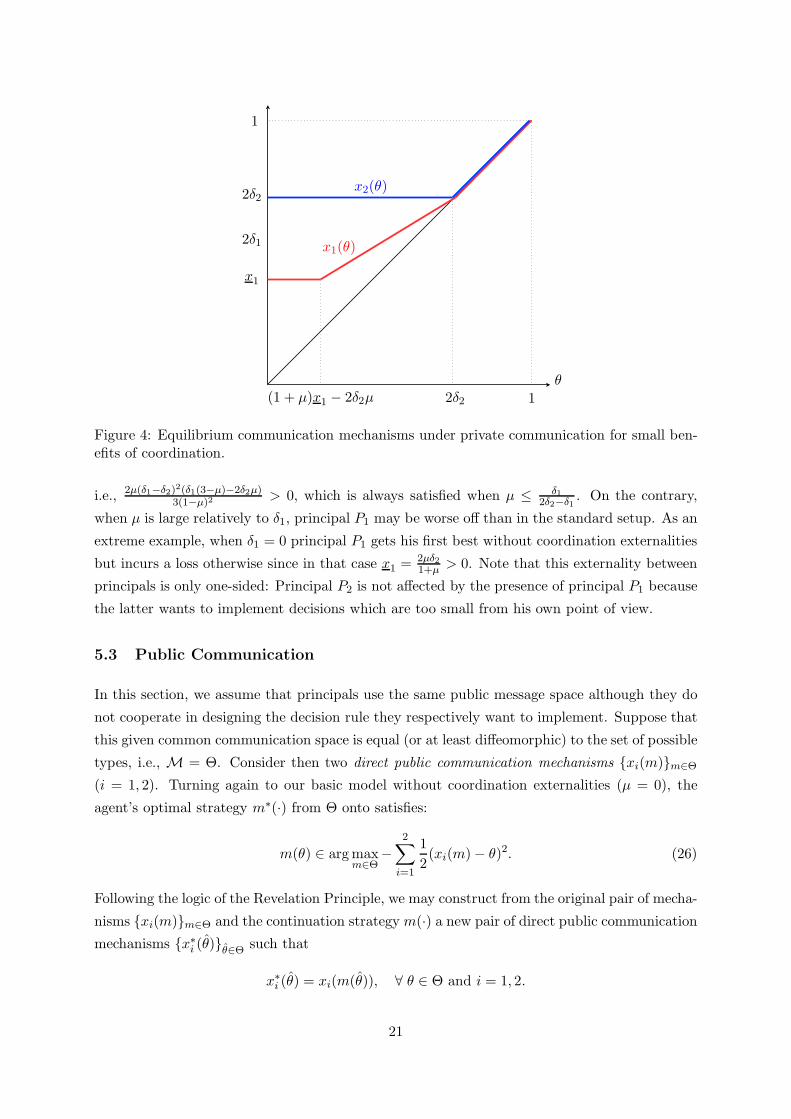
2δ2(1 + µ)x1 − 2δ2µ

x1

2δ2

x1(θ)2δ1

x2(θ)

θ1

1

Figure 4: Equilibrium communication mechanisms under private communication for small ben-efits of coordination.

i.e., 2µ(δ1−δ2)2(δ1(3−µ)−2δ2µ)3(1−µ)2

> 0, which is always satisfied when µ ≤ δ12δ2−δ1

. On the contrary,

when µ is large relatively to δ1, principal P1 may be worse off than in the standard setup. As an

extreme example, when δ1 = 0 principal P1 gets his first best without coordination externalities

but incurs a loss otherwise since in that case x1 = 2µδ21+µ

> 0. Note that this externality between

principals is only one-sided: Principal P2 is not affected by the presence of principal P1 because

the latter wants to implement decisions which are too small from his own point of view.

5.3 Public Communication

In this section, we assume that principals use the same public message space although they do

not cooperate in designing the decision rule they respectively want to implement. Suppose that

this given common communication space is equal (or at least diffeomorphic) to the set of possible

types, i.e., M = Θ. Consider then two direct public communication mechanisms {xi(m)}m∈Θ

(i = 1, 2). Turning again to our basic model without coordination externalities (µ = 0), the

agent’s optimal strategy m∗(·) from Θ onto satisfies:

m(θ) ∈ arg maxm∈Θ

−2∑

i=1

1

2(xi(m) − θ)2. (26)

Following the logic of the Revelation Principle, we may construct from the original pair of mecha-

nisms {xi(m)}m∈Θ and the continuation strategy m(·) a new pair of direct public communication

mechanisms {x∗i (θ)}θ∈Θ such that

x∗i (θ) = xi(m(θ)), ∀ θ ∈ Θ and i = 1, 2.

21

This means that, at any putative equilibrium with pure strategy we may consider, the pair

of direct public communication mechanisms {x∗1(·), x∗2(·)} offered at this equilibrium is jointly

incentive compatible and satisfies:

θ ∈ arg maxθ∈Θ

−2∑

i=1

1

2(x∗i (θ) − θ)2. (27)

This is a rather weak statement of the Revelation Principle. Indeed, off the equilibrium

path, each principal may want to offer another communication mechanism which corresponds

to a non-truthful public communication strategy by the agent. This is a general point of the

common agency literature (see Martimort and Stole, 2002 for instance) that applies here also.

Formally, for any possible deviation by principal i, say a communication mechanism xi(·) :

Θ → R, the agent’s communication strategy in the continuation satisfies now:

m∗(θ) ∈ arg maxm∈Θ

−1

2(xi(m) − θ)2 − 1

2(x∗−i(m) − θ)2. (28)

For each of those deviations, the principal may alternatively offer the direct communication

mechanism {xi(θ)}θ∈Θ defined as

xi(θ) = xi(m∗(θ)) ∀ θ ∈ Θ.

With this observation, (28) implies also that the following incentive constraints hold:

θ ∈ arg maxθ∈Θ

−1

2(xi(θ) − θ)2 − 1

2(x∗−i(m

∗(θ)) − θ)2. (29)

Those incentive constraints can be interpreted as follows. Everything happens as if principal Pi

could indeed deviate by offering an extended direct mechanism {xi(θ),m∗(θ)}

θ∈Θ to the agent.

The agent then privately communicates his type to that deviating principal by sending a message

θ who then recommends first which decision xi(θ) the agent should adopt and, second which

public message m∗(θ) the agent should sent to the non-deviating principal −i.

If there exists any pure strategy equilibrium with direct public communication mechanisms

{x∗1(·), x∗2(·)} between the principals, with (without loss of generality) a truthful strategy being

played by the agent in the continuation, it must be that none of these principals may want to

deviate to an alternative extended direct mechanism inducing possibly a non-truthful contin-

uation. It turns out that such a condition is highly constraining. Indeed, the public message

m∗(·) can be used by the deviating principal, say Pi, as a second screening variable on top of

the decision rule xi(·). This second variable facilitates information revelation towards principal

i but possibly comes at the cost of inducing “public lies”. Following the logic of Section 4,

adding more screening instruments may facilitate deviations compared with the case of private

communication.

Example 3 As an illustration, consider the optimal pair of private mechanisms when δ1 =

0 < δ2 < 1/2, i.e., x∗1(θ) = θ and x∗2(θ) = max{θ, 2δ2}. Since this pair of mechanisms induces

22

truthtelling to both principals under private communication, it also induces truthtelling under

public communication. Consider the deviation by principal P2 to the mechanism x2(θ) = θ+ δ2.

This deviation induces the agent to underreport his type, and the associated extended direct

mechanism is:

m∗(θ) = arg minm∈Θ

(m− θ)2 + (m+ δ2 − θ)2 = max{θ − δ2/2, 0}

and x2(θ) = x2(m∗(θ)) = θ + δ2/2. This deviation is always profitable for principal P2 because

∫ 1

0(x∗2(θ) − θ − δ2)

2dθ >

∫ 1

0(x2(m

∗(θ)) − θ − δ2)2dθ ⇐⇒ δ2 < 9/16.

We will show below that, more generally, no pair of (continuous and piecewise differentiable)

mechanisms can prevent a profitable deviation by one of the principals.

Remark 1 The set of extended direct mechanisms {xi(θ),m∗(θ)}

θ∈Θ may allow more deviations

than what is available with direct communication mechanisms. In other words, although (28)

implies (29) the reverse is not true. Think indeed of a deviation in extended direct mechanisms

that would require the agent to send a fixed public message m∗(θ) = m∗ ∈ Θ independently of

his own type θ but that would require full separation in terms of the decisions, i.e., xi(θ) being

now injective. Clearly, there would not exist a direct communication mechanism {xi(m)}m∈Θ

that could replicate such outcome. This is only possible when the m∗(·) induced by the deviation

is itself injective. This points at the fact that the set of deviations with direct communication

mechanisms leads to an open set. Our response to this difficulty is to consider first deviations

in the larger set defined by (29) and then show that such a deviation can be approximated as

closely as wanted by using a injective recommendation m∗(·).

From now on, we adopt an approach close to that performed in Section 4. We first look for

the incentive properties of the information rent profile that principal i may induce by deviating

within the class of extended direct mechanisms. Second, we optimize within that set. This will

lead us to our impossibility result.

Fix the direct public communication mechanism {x∗−i(m))}m∈Θ offered at a putative pure

strategy equilibrium by principal −i. We assume that this mechanism is continuous and piece-

wise differentiable.30 For a given extended mechanism {xi(θ),m∗(θ)}

θ∈Θ, define the agent’s

information rent U(θ) as:

U(θ) = maxθ∈Θ

−1

2(xi(θ)− θ)2−

1

2(x∗−i(m

∗(θ))− θ)2 = −1

2(xi(θ)− θ)2−

1

2(x∗−i(m

∗(θ))− θ)2. (30)

Using the Envelope Theorem, we immediately obtain

U(θ) = xi(θ) + x∗−i(m∗(θ)) − 2θ, (31)

30A remark is in order here. In the case of a cooperative design, we derive the differentiability properties of thecommunication mechanisms from the incentive compatibility constraints. This is no longer possible to proceedsimilarly jointly for both principals since the differentiability properties of one mechanism may follow from thoseof the other. We just look for such differentiable equilibria right away.

23

with the second-order condition for incentive compatibility being now expressed as

U(θ) = xi(θ) + m∗(θ)x∗−i(m∗(θ)) − 2 ≥ −2. (32)

From (30) and (31), we immediately derive a second order equation in x∗−i(m∗(θ)), namely:

U(θ) = −1

2(U(θ) − (x∗−i(m

∗(θ)) − θ))2 − 1

2(x∗−i(m

∗(θ)) − θ)2. (33)

Having a real solution to this equation requires U(θ) ≤ 0 and, keeping the lowest such solution,31

we get:

x∗−i(m∗(θ)) − θ =

U(θ)

2−

√

−U(θ) − U2(θ)

4and xi(θ) − θ =

U(θ)

2+

√

−U(θ) − U2(θ)

4. (34)

This equation in fact implicitly defines the public message m∗(θ) that helps principal i to im-

plement a rent profile U(θ) when considering a deviation. Given the range of x∗−i(·), Imx∗−i,

this implementability condition can as well be written as:

U(θ)

2−

√

−U(θ) − U2(θ)

4+ θ ∈ Imx∗−i. (35)

Using (34), we may rewrite principal i’s payoff in each state of nature θ as:

−1

2δ2i − 1

2

U(θ)

2+

√

−U(θ) − U2(θ)

4

2

+ δi

U(θ)

2+

√

−U(θ) − U2(θ)

4

.

Neglecting the second-order condition (32), we can express principal i’s problem in looking for

an optimal deviation as:

(Ppci ) : max

U(·)

∫ 1

0Li(U(θ), U(θ))dθ, subject to (35),

where

Li(U(θ), U (θ)) = −1

2

U(θ)

2+

√

−U(θ) − U2(θ)

4

2

+ δi

U(θ)

2+

√

−U(θ) − U2(θ)

4

.

Note that Li(s, v) is a concave function of (s, v) although it may not be differentiable everywhere

especially at points where U(θ)+ U2(θ)4 = 0 if any such θ exists. Equipped with this formulation,

we can now show the following proposition:

Proposition 6 With conflicting principals and public communication, there does not exist any

pure strategy equilibrium of the public communication game with continuous and piecewise dif-

ferentiable direct mechanisms.

31We could keep the highest such solution by permuting the role of principal i and −i.

24

5.4 Cheap-Talk with Multiple Audiences

One possibility to restore the existence of an equilibrium is to consider the situation in which the

principals can no longer commit to a decision rule. More precisely, assume that communication

takes place via unilateral cheap talk, from the agent to the principals. The timing of this

communication game is as follows:

⋆ First, the agent learns his type θ ∈ Θ.

⋆ Second, the agent sends a (public or private) message to the principals.

⋆ Third, each principal chooses an action as a function of the message he received.

A strategy for principal Pi is a mapping σi : Θ → R, where σi(θ) is the action chosen by

principal Pi when he has received the message θ. Under private communication, a strategy for

the agent is a pair (σ1A, σ

2A), where σi

A : Θ → Θ and σiA(θ) is the message privately observed by

principal Pi when the agent’s type is θ. A strategy for the agent under public communication is

defined similarly, with the restriction that principals P1 and P2 observe the same public message

σ1A(θ) = σ2

A(θ) when the agent’s type is θ.

Since there is a one-to-one correspondence between the message received by principal Pi and

his optimal action, every equilibrium is outcome equivalent to a partitional equilibrium, in which

the agent’s strategy takes the following form for some K ∈ N∗+: σi

A(θ) = m1 if θ ∈ [0, yi1), . . . ,

σiA(θ) = mk if θ ∈ [yi

k−1, yik), . . . , σi

A(θ) = mK if θ ∈ [yiK−1, 1], with 0 < yi

1 < · · · < yiK−1 <

yK = 1, mk 6= mk′ for k 6= k′, and the restriction σ1A = σ2

A under public communication.

The following proposition shows that whatever the communication protocol (public or pri-

vate), equilibrium outcomes take exactly the same form as in Crawford and Sobel (1982), with

the bias parameter being δi in the private communication game with principal Pi, and δ = δ1+δ22

in the public communication game. Notice that for this characterization we do not impose any

assumption on δ1 and δ2.

Proposition 7 (Cheap Talk: Equilibrium Characterization)

• Under private communication, there is a partitional equilibrium with Ki different messages

sent privately to principal Pi and

yik =

k

Ki+ 2kδi(Ki − k), i = 1, 2, k = 1, . . . Ki, (36)

if and only if |δi| ≤ 12Ki(Ki−1) .

• Under public communication, there is a partitional equilibrium with K different messages

sent publicly to both principals and

yk =k

K+ 2kδ(K − k), k = 1, . . . K, (37)

25

if and only if |δ| ≤ 12K(K−1) .

A generalization of the phenomenon already identified by Farrell and Gibbons (1989) ap-

pears here. Indeed, in a model with binary actions and states, these authors show that full

revelation of information to both principals under private communication implies full revela-

tion of information in public, but that the reverse in not true. More specifically, if there is a

Ki-partitional equilibrium with each principal Pi in private, with K1 = K2 = K, then there is

also a K-partitional equilibrium in public, but the reverse is not true. As an extreme example,

take δ1 = −δ2 > 1/4. Then, the unique equilibrium outcome under private communication

is non-revealing while there is a K-partitional equilibrium under public communication for all

K ∈ N∗+.

The following proposition characterizes players’ (ex-ante) preferences over the two communi-

cation protocols depending on the configuration of the biases δ1 and δ2. To allow this comparison,

we consider the “most informative” equilibria in both cases, i.e., those equilibria with the largest

number of different messages sent by the agent.32

Proposition 8 (Cheap Talk: Welfare) Consider the most informative Ki-partitional equi-

librium outcome with principal Pi under private communication, for i = 1, 2, and the most

informative K-partitional equilibrium outcome under public communication. For every i = 1, 2,

we have:

If |δ| < |δi| and max{Ki,K} > 1, then principal Pi is strictly better off under public com-

munication than under private communication.

If |δ| > |δi| and max{Ki,K} > 1, then principal Pi is strictly worse off under public com-

munication than under private communication.

If |δ| < |δi| for i = 1, 2 and max{K1,K2,K} > 1, then the agent is strictly better off under

public communication than under private communication.

If |δ1| < |δ| < |δ2|, then the agent may be strictly better off or strictly worse off under public

communication than under private communication.

In particular, players are indifferent between public and private communication only when

principals are perfectly symmetric (δ1 = δ2) or when there is no communication (K1 = K2 =

K = 1). Notice also that the ex ante expected social welfare, defined as the sum of all three

players’ expected utilities, can always be identified with the agent’s expected utility.

32This equilibrium selection can be justified with several perturbations of the cheap talk game. See, e.g., Chenet al. (2008).

26

6 Conclusion

Let us briefly wrap the main findings of our analysis and point out a few directions for further

research.

First, multi-dimensional communication mechanisms exhibit quite different features than the

simple delegation sets found in the one-dimensional case when they are jointly designed by co-

operating principals. The possibility of trading off distortions on each dimension of the agent’s

activity leads to full separation and makes simple delegation sets suboptimal. However, the loss

of using simple mechanisms that generalize those delegation sets might be quite small when the

principals’ objectives are not too different. It would be worth investigating the cooperative de-

sign of communication mechanisms in more complex environments allowing more general utility

functions or type distributions. This research program is likely to meet strong technical diffi-

culties coming from the impossibility to learn much from the Euler-Lagrange equation beyond

the quadratic utility function/uniform type distribution investigated here. These difficulties will

have to be overcome by unattractive numerical methods. Nevertheless, we feel quite confident

about the robustness of our findings and especially on the increased scope for full separating

allocations.

Second, we have found that delegation sets remain optimal in a non-cooperative environment

as long as communication between the agent and each of his principals remains private. However,

such non-cooperative design of delegation sets might have to take into account any existing

coordination benefit from having the actions controlled by the principals jointly performed by

the agent. Such settings lead to one-sided externality between principals. Other forms of

externalities between principals (be they only indirect through the agent’s utility function or

also more direct) could certainly be handled with the same techniques as the ones we used to

get this result.

Third, public communication between competing principals opens possibilities for strategic

gaming where each principal tries to affect the publicly communicated report to his own advan-

tage. Far from helping screening as in the cooperative setting, the mere possibility of enlarging

the screening abilities of each principal by having him play on what is publicly communicated

by the agent makes impossible to sustain any pure strategy equilibrium with continuous mech-

anisms. Again, there is no longer any scope for delegation sets to emerge in such contexts.

An open and extraordinarily difficult question is the form that any mixed strategy equilibria

might have in such context. This non-existence result suggests that the alternative cheap talk

timing where principals only react to the agent’s announcement may have quite an appeal. We

investigated equilibria of the public and private communication games in such environments.

27

Appendix

Proof of Proposition 1. Given the class of communication mechanisms we consider, the

optimization problem of principal Pi can be written as

min(θ∗i ,θ∗∗i )

∫ θ∗i

0(θ∗i − θ − δi)

2dθ +

∫ θ∗∗i

θ∗i

(δi)2dθ +

∫ 1

θ∗∗i

(θ∗∗i − θ − δi)2dθ,

when θ∗i < θ∗∗i ≤ 1, and

minθ∗i

∫ 1

0(θ∗i − θ − δi)

2dθ,

when θ∗i = θ∗∗i . This yields θ∗i = 2δi and θ∗∗i = 1 when δi ≤ 1/2.

Proof of Lemma 1. We proceed along the lines of Clarke (1990, Chapter 4) and especially

Theorem 1.1.3 therein. We first observe that:

1. L∆(s, v) is B-measurable where B denotes the σ−algebra of subsets of R− × R.

2. L∆(s, v) is continuous and thus lower-hemi continuous.

3. L∆(s, v) is concave in (s, v).

Define now the Hamiltonian H(s, p) as:

H(s, p) = maxv∈R

{pv + L∆(s, v)} = maxv∈R

(p+ δ)v + s+ ∆

√

−s− v2

2.

The maximum above is achieved for

v∗ = 2(p+ δ)

√

−2s

2(p + δ)2 + ∆2,

which yields

H(s, p) = s+√

−2s(2(p + δ)2 + ∆2)

This implies the following inequality :

H(s, p) ≤ −s+ ∆√−2s+

√

−4s(p+ δ)2 = |s| + ∆√

2|s| + 2|p + δ|√

|s|.

Using now that√

|s| ≤ 1 + |s|2 and that |p+ δ| ≤ |p| + δ, we obtain finally:

H(s, p) ≤ ∆√

2 + 2δ + |s|(

1 + δ +∆√2

+ |p|)

. (A.1)

This is a “growth” condition on the Hamiltonian as requested in Clarke (1990, Theorem 1.1.3).

Lemma 3 Clarke (1990). Assume that L∆(·) satisfied conditions [1.] to [3.] above, that H(·)satisfies the “growth” equation (A.1) and that

∫ 10 L∆(U0(θ), U0(θ))dθ is finite for at least one

admissible arc U0(θ). Then, problem Pc∆ has a solution.

28

It remains to show that∫ 10 L∆(U0(θ), U0(θ))dθ is finite for at least one admissible arc U0(θ).

Take U0(θ) = 0 which corresponds to decisions x10(θ) = x20(θ) = θ. This arc does the job and

yields∫ 10 L∆(U0(θ), U0(θ))dθ = 0.

Proof of Lemma 2. Since the functional L∆(·) does not depend on θ, we can obtain a first

quadrature of (15) using Gelfand and Fomin (1991, Chapter 1, p. 19) on any interval where

U(θ) + U2(θ)4 < 0 as:

L∆(U(θ, λ), U (θ, λ)) − U(θ, λ)∂L

∂U(U(θ, λ), U (θ, λ)) = −λ (A.2)

where a priori λ ∈ R and where we make explicit the dependence of the solution on this param-

eter. We obtain immediately:

U(θ, λ) + δU(θ, λ) + ∆

√

−U(θ, λ) − U2(θ, λ)

4− U(θ, λ)

δ − ∆U(θ, λ)

4

√

−U(θ, λ) − U2(θ,λ)4

= −λ.

Simplifying yields:

U(θ, λ)

1 − ∆√

−U(θ, λ) − U2(θ,λ)4

= −λ.

Solving for U(θ, λ) yields

U2(θ, λ) = −4

(

U(θ, λ) + ∆2

(

U(θ, λ)

U(θ, λ) + λ

)2)

, (A.3)

which requires −∆2(

U(θ,λ)U(θ,λ)+λ

)2≥ U(θ, λ) or (U(θ, λ)+λ)2+∆2U(θ, λ) ≥ 0 given that U(θ, λ) ≤

0 since by definition the agent’s information rent is the sum of two negative terms. Solving the

second-order equation (A.3) and keeping the positive root only,33 we get (17). When U(θ, λ) > 0,

differentiating (17) with respect to θ yields

U(θ, λ) +U(θ, λ)

(

1 + 2λ∆2 U(θ,λ)(U(θ,λ)+λ)3

)

√

−U(θ, λ) − ∆2(

U(θ,λ)U(θ,λ)+λ

)2= U(θ, λ) + 2

(

1 + 2λ∆2 U(θ, λ)

(U(θ, λ) + λ)3

)

= 0 (A.4)

Hence, on any interval where U(θ, λ) > 0, the second-order condition (12) can be written as

0 ≤ U(θ, λ) + 2 = −4λ∆2 U(θ, λ)

(U(θ, λ) + λ)3. (A.5)

Since U(θ, λ) ≤ 0 holds, λ ≤ 0 implies also U(θ, λ) + λ ≤ 0 and then (A.5) holds which puts

the requested restriction on the admissible solutions to (17). Finally, note that the second-order

condition (12) holds obviously on any interval where instead U(θ, λ) = 0.

33Since it corresponds to a aggregate decisions x(θ) biased towards the merged principal, namely x(θ) ≥ 2θ (seeequation (11)).

29

Proof of Proposition 2. The structure of the proof is as follows. First, we derive the necessary

free end-point conditions (16) and the characterization given in Lemma 2. Sufficiency follows.

Necessity: Define the function

P (x) =−x((x+ λ)2 + ∆2x)

(x+ λ)2.

For x < 0, P (x) > 0 if and only if the second degree polynomial (x+ λ)2 + ∆2x is everywhere

positive. This is so when

λ < −∆2

4.

When that condition holds, the differential equation (17) is Lipschitz at any point where

U(θ, λ) < 0 and thus it has a single solution at any such point. Moreover, a solution U(θ, λ) is

then everywhere increasing on the whole domain where U(θ, λ) < 0. As a result, the differential

equation (17) is everywhere Lipschitz when U(1, λ) < 0 which turns out to be the case for the

path we derive below.

The necessary free end-points conditions (16) can be rewritten for an optimal path as:

−δ + ∆U∗(θ)

4

√

−U∗(θ) − (U∗(θ))2

4

|θ=0,1 = 0.

Using (17) to express U∗(θ), those conditions can be simplified so that U∗(0) and U∗(1) solve

indeed the following second-order equation in U :

(U + λ)2 = −(∆2 + 4δ2)U (A.6)

Assume now that

λ > −∆2

4− δ2.

Then (A.6) admits two solutions U(0, λ) and U(1, λ) which are respectively given by

U∗(0, λ) = −λ− 1

2

(

∆2 + 4δ2 +√

(∆2 + 4δ2)2 + 4λ(∆2 + 4δ2))

(A.7)

and

U∗(1, λ) = −λ− 1

2

(

∆2 + 4δ2 −√

(∆2 + 4δ2)2 + 4λ(∆2 + 4δ2))

. (A.8)

Equations (19) and (20) follow when λ = λ∗. Note in particular that (A.6) implies that both

solutions are negative.

The last step is to show that there exits λ∗ ∈ (−∆2

4 − δ2,−∆2

4 ) such that the corresponding

path U∗(θ) = U(θ, λ∗) solving (17) and starting from U(0, λ∗) = U∗(0, λ∗) = U∗(0) given by

(19) reaches U(1, λ∗) = U∗(1, λ∗) = U∗(1) given by (19). This requires to find a solution λ∗ to

the equation

ϕ(λ) = ψ(λ),

30

where

ϕ(λ) = U∗(1, λ) − U∗(0, λ) =√

(∆2 + 4δ2)2 + 4λ(∆2 + 4δ2),

and

ψ(λ) =

∫ 1

0U(θ, λ)dθ =

∫ 1

02

√

−U(θ, λ) − ∆2

(

U(θ, λ)

U(θ, λ) + λ

)2

dθ,

where the path U(θ, λ) starts from the initial condition U(0, λ) = U∗(0, λ). Note that both

ϕ(·) and ψ(·) are continuous in λ. It is clear that ϕ(λ) is strictly increasing in λ with, for

λ1 = −∆2

4 − δ2 and λ2 = −∆2

4 ,

ϕ (λ1) = 0 < 2δ√

∆2 + 4δ2 = ϕ (λ2) .

On the other hand, note that

ψ (λ1) > 0 = ϕ (λ1) , (A.9)

since the path U (θ, λ1) starting from U∗(0, λ1) is strictly increasing. Moreover, for λ2, (17) can

be rewritten as:

U(θ, λ2) = 2√

−U(θ, λ2)|U(θ, λ2) − λ2||U(θ, λ2) + λ2|

. (A.10)

The path solving (A.10) and starting at U∗(0, λ2) (note that U∗(0, λ2) < λ2 < U∗(1, λ2)) is

strictly increasing everywhere and cannot cross the boundary U = λ2 because the only solution

to (A.10) such that U(θ1) = λ2 for a given θ1 > 0 is such that U(θ) = λ2 for all θ since the

right-hand side of (A.10) satisfies a Lipschitz condition at any point U(θ, λ2) away from zero;

a contradiction with U∗(0, λ2) < λ2. From that, we deduce U(θ, λ2) < λ2 for all θ. Hence, the

following sequences of inequalities holds:

ψ (λ2) =

∫ 1

0U(θ, λ2)dθ < λ2 − U∗(0, λ2) = λ2 − U∗(1, λ2) + ϕ (λ2) .

Finally, we get:

ψ (λ2) < ϕ (λ2) . (A.11)

Gathering Equations (A.9) and (A.11) yields the existence of λ∗ ∈ (λ1, λ2) such that ϕ(λ∗) =

ψ(λ∗).

Sufficiency: Sufficiency follows from Clarke (1990, Chapter 4, Corollary p. 179). Indeed, as we

have shown above in the proof of Lemma 1, L∆(·) satisfies the convexity assumption. Moreover,

the Hamiltonian

H(s, p(θ)) = s+√

−2s(2(p(θ) + δ)2 + ∆2),

is a concave function of s where we denote p(θ) an arc satisfying the necessary conditions:

−p(θ) =∂H

∂U(θ, U∗(θ), p(θ)) = 1 −

√

−(2(p(θ) + δ)2 + ∆2)

2U∗(θ), (A.12)

U∗(θ) =∂H

∂p(θ, U∗(θ), p(θ)) = −(p(θ) + δ)

√

U∗(θ)

−2(2(p(θ) + δ)2 + ∆2), (A.13)

31

p(0) = p(1) = 0. (A.14)

It can be checked that conditions (A.12) and (A.13) are altogether equivalent to (15) whereas

(A.14) is equivalent to the free-end points conditions (16).

Proof of Corollary 1. First observe that

x∗(0) = U∗(0) = 2

√

−U∗(0)((U∗(0) + λ∗)2 + ∆2U∗(0))

|U∗(0) + λ∗| .

Using (19), we get:

x∗(0) = 4δ|U∗(0)|

|U∗(0) + λ∗| < 4δ.

Finally, we obviously have x∗(θ) − 2θ = U∗(θ) > 0 for all θ.

Proof of Corollary 2. The first property directly follows from (22). Now, from the incentive

constraint (6) and the first property of the corollary we get the second property. Next, using (22)

we have x∗1(0) > 0 if and only if

U∗(0)

2> ∆

(

U∗(0)

U∗(0) + λ∗

)

.

Using (17) and simplifying we get

2∆2U∗(0) > −(U∗(0) + λ∗)2,

i.e., by (A.6), 2∆2 < ∆2 + 4δ2, which is always satisfied. x∗2(0) < 0 follows now from the second

property of the corollary. The last property is proved similarly.

Proof of Corollary 3. The proof is immediate and is omitted.

Proof of Proposition 3. Consider the mechanism {x∗1(θ), x∗2(θ)}θ∈Θ which can be written as:

x∗1(θ) =

{

θ − ∆2 if θ ≥ 2δ

2δ − ∆2 otherwise

and x∗2(θ) =

{

θ + ∆2 if θ ≥ 2δ

2δ + ∆2 otherwise.

(A.15)

The corresponding information rent for the agent satisfies:

U∗(θ) =

{

−∆2

4 if θ ≥ 2δ

−(2δ − θ)2 − ∆2

4 otherwise.(A.16)

Note in particular that we have:

−U∗(θ) − ( ˙U∗(θ))2

4=

∆2

4for all θ.

Using these expression, we get:

∫ 1

0L∆(U∗(θ), ˙U∗(θ)))dθ =

∫ 2δ

0(2δ(2δ − θ) − (2δ − θ)2)dθ +

∆2

4=

4δ3

3+

∆2

4. (A.17)

32

We also have

∫ 1

0L∆(U∗(θ), U∗(θ))dθ ≤

∫ 1

0

L0(U∗(θ), U∗(θ)) + ∆

√

−U∗(θ) − [U∗(θ)]2

4

dθ

=4δ3

3+ ∆2

∫ 1

0

|U∗(θ)||U∗(θ) + λ∗|dθ

where the last equality follows from (17). The last inequality implies:

∫ 1

0L∆(U∗(θ), U∗(θ))dθ ≤ 4δ3

3+ ∆2. (A.18)

Putting together (A.17) and (A.18) yields the result.

Proof of Proposition 4. The proof is immediate and is omitted.

Proof of Proposition 5. Following the methodology of Martimort and Stole (2007), let us

define the agent’s indirect utility function U(xi, θ) as:

U(xi, θ) = maxx−i∈D−i

U(xi, x−i, θ).

Similarly, we denote x−i(xi, θ) the agent’s best choice in D−i given his type and the decision

that Pi would like to induce as

x−i(xi, θ) = arg maxx−i∈D−i

U(xi, x−i, θ).

By concavity of U(·), x−i(xi, θ) is uniquely defined as

x−i(xi, θ) = max

{

θ + µxi

1 + µ, x−i

}

. (A.19)

Defining x∗i (θ) = 1µ((1 + µ)x−i − θ), we have

U(xi, θ) =

{

− 1+2µ2(1+µ) (xi − θ)2 if xi ≥ x∗i (θ)

−12(xi − θ)2 − 1

2(x−i − θ)2 − µ2 (xi − x−i)

2 otherwise.(A.20)

Note that U(xi, θ) is continuous in xi although not differentiable everywhere.

Incentive compatibility at differentiability points: With these definitions, we can rewrite the

incentive compatibility conditions vis-a-vis principal Pi as:

θ ∈ arg maxθ

U(xi(θ), θ) = arg maxθ

U(xi(θ), x−i(xi(θ), θ), θ). (A.21)

The first-order condition for the agent’s incentive problem can thus be written at any differ-

entiability point as:

0 =

{

xi(θ) (xi(θ) − θ) if xi ≥ x∗i (θ)

xi(θ)(

(1 + µ)xi(θ) − θ − µx−i

)

otherwise.(A.22)

33

The corresponding second-order condition for the agent’s incentive problem remains at any

differentiability point

xi(θ) ≥ 0. (A.23)

Observe that (A.22) shows that any continuous xi(θ) has either flat parts, or is such that

xi(θ) = θ when xi(θ) = θ ≥ x∗i (θ) (i.e., when θ ≥ x−i) and xi(θ) = 11+µ

(θ + µx−i) when

xi(θ) ≤ x∗i (θ) (i.e., when θ ≤ x−i).

Best-response in the class of continuous mechanisms: We will use the characterization of contin-

uous decision rules given above to describe an equilibrium in which x2 ≥ x1. That equilibrium

turns out to be unique.

When x1(θ) is continuous and (1 + µ)x1 − µx2 ∈ [0, x2], principal P1 expected payoff’s can

be written as:

− 1

2

(

∫ (1+µ)x1−µx2

0(x1 − θ − δ1)

2dθ

+

∫ x2

(1+µ)x1−µx2

(

1

1 + µ(θ + µx2) − θ − δ1

)2

dθ +

∫ 1

x2

δ21dθ

)

.

(A.24)

Optimizing with respect to x1 yields the following first-order condition:

∫ (1+µ)x1−µx2

0(x1 − θ − δ1)dθ = 0.

Simplifying, we obtain the following best-response:

x1 =1

1 − µ(2δ1 − µx2), (A.25)

as long as µx2 ≤ (1 + µ)δ1 ≤ x2.

Turning now to principal P2’s best-response. Given the characterization of incentive com-

patibility given above and the fact that we are looking for an equilibrium such that x2 ≥ x1,

principal P2 expected payoff’s can be written as:

−1

2

(

∫ x2

0(x2 − θ − δ2)

2dθ +

∫ 1

x2

δ22dθ

)

.

Optimizing yields the following best-response in the class of continuous mechanisms:

x2 = 2δ2. (A.26)

Hence, Imx2(·) = D2 = [2δ2,+∞).

Equilibrium: Gathering (A.25) and (A.26) yields finally (24). Conditions (25) are then obtained

when x1 is at a corner, i.e., (1 + µ)x1 − µx2 = 0.

Proof of Proposition 6. We first prove that there does not exist any equilibrium with one

principal, P−i, offering a separating allocation x−i(·) over an interval [θ0, θ1] ⊆ [0, 1]. Suppose

34

the contrary. Since each principal finds optimal to induce a message m∗(θ) = θ for all θ ∈ Θ, on

such an interval of separation it must necessarily be that the implementability condition (35) is

slack for principal Pi. This implies that principal Pi would like to implement a rent profile U(θ)

that maximizes pointwise the maximand in (Ppci ) over the interval [θ0, θ1], i.e., such that:

U(θ)

2+

√

−U(θ) − U2(θ)

4= arg max

φ−φ

2

2+ δiφ = δi, (A.27)

which is achieved with U(θ) = δ2i and decision rules x∗i (θ) = θ + δi and x∗−i(m∗(θ)) = θ − δi.

The mechanism x∗i (θ) being separating over that interval, a symmetric reasoning yields x∗−i(θ) =

θ + δ−i and x∗i (m∗(θ)) = θ − δ−i. This is impossible when δ2 6= −δ1 and when m∗(θ) = θ as

requested in a pure strategy equilibrium.

Since there is no interval of separation, each principal must offer a pooling mechanism over

the whole interval [0, 1]. But in that case, principal Pi offers as a best response his optimal private

mechanism. This mechanism is separating over the interval [2δi, 1], which yields a contradiction.

Proof of Proposition 7. We show the proposition under public communication (the proof

is similar and well known under private communication). In a K-partitional equilibrium, the

optimal action of principal Pi after message mk is σi(mk) =yk−1+yk

2 + δi. The best response of

the agent is such that for all k = 1, . . . ,K−1, he is indifferent between sending message mk and

mk+1 when his type is θ = yk. After some simplifications, this yields yk+1−yk = yk −yk−1−4δ,

so yk = ky1 − 2k(k − 1)δ. In particular, yK = Ky1 − 2K(K − 1)δ = 1, i.e., y1 = 1K

+ 2(K − 1)δ,

which gives the threshold of Equation (37). This K-partitional equilibrium is feasible if y1 > 0

and yK−1 < 1, i.e., − 12K(K−1) < δ < 1

2K(K−1) .

Proof of Proposition 8. When for i = 1, 2, a Ki-partitional communication strategy σiA is

played with principal Pi in private, his ex-ante expected equilibrium payoff is given by

EV (Ki, δi) = −Ki∑

k=1

∫ yik

yik−1

(σi(mk) − θ − δi)2 dθ = − 1

12

Ki∑

k=1

(yik − yi

k−1)3

= − 1

12

Ki∑

k=1

(1/Ki − 2δi(2k −Ki − 1))3 = − 1

12K2i

− δ2i (K2i − 1)

3, (A.28)

and the ex-ante expected equilibrium payoff of the agent is given by

EV (K1, δ1) + EV (K2, δ2) − δ21 − δ22 . (A.29)

Similarly, when a K-partitional communication strategy σA is played in public, the ex-ante

expected equilibrium payoff of principal Pi is given by EV (K, δ), and the ex-ante expected

equilibrium payoff of the agent is given by

2EV (K, δ) − δ21 − δ22 . (A.30)

35

If |δ| < |δi|, then by Proposition 7 the most informative Ki-partitional equilibrium under

private communication with principal Pi and the most information K-partitional equilibrium

under public communication are such that Ki ≤ K. Principal Pi is strictly better off under

public communication if and only if EV (K, δ) > EV (Ki, δi), i.e.,

1

4K2+ δ2(K2 − 1) <

1

4K2i

+ δ2i (K2i − 1).

This inequality is immediate when K = Ki 6= 1. When Ki < K, a sufficient condition for the

inequality to be satisfied is

1

4K2+ δ2(K2 − 1) <

1

4K2i

+ δ2(K2i − 1),

i.e., |δ| < 12KKi

. Since Ki ≤ K − 1, this condition is implied by |δ| < 12K(K−1) , which is exactly

the condition for a K-partitional equilibrium to exist under public communication.

Similarly, if |δ| > |δi|, then Ki ≥ K and principal Pi is strictly worse off under public

communication if and only if

1

4K2+ δ2(K2 − 1) >

1

4K2i

+ δ2i (K2i − 1),

which is immediate when K = Ki 6= 1. When Ki > K, a sufficient condition for the inequality

to be satisfied is |δi| < 12Ki(Ki−1) , which is exactly the condition for a Ki-partitional equilibrium

to exist under private communication with principal Pi.

If |δ| < |δi| for i = 1, 2 it is obvious from the analysis above and the expressions of the agent’s

expected payoff given by Equations (A.29) and (A.30) that he is strictly better off under public

than under private communication.

If |δ1| < |δ| < |δ2|, then it is easy to construct examples in which the agent is strictly better

off under public communication (e.g., with K = K1), or in which he is strictly worse off (e.g.,

with K = K2).

References

Alonso, N. and R. Matouschek (2008): “Optimal Delegation,” Review of Economic Studies,

forthcoming.

Armstrong, M. (1994): “Delegation and Discretion,” Discussion Papers in Economics and

Econometrics 9421, University of Southampton.

Arnott, R. and J. Stiglitz (1988): “Randomization with Asymmetric Information,” Rand

Journal of Economics, 19, 344–362.

Baron, D. (2000): “Legislative Organization with Informational Committees,” American Jour-

nal of Political Sciences, 44, 485–505.

36

Battaglini, M. (2002): “Multiple Referrals and Multidimensional Cheap Talk,” Econometrica,

70, 1379–1401.

Chen, Y., N. Kartik, and J. Sobel (2008): “Selecting Cheap-Talk Equilibria,” Economet-

rica, 76, 117–136.

Clarke, F. H. (1990): Optimization and Nonsmooth Analysis, SIAM. Philadelphia.

Crawford, V. P. and J. Sobel (1982): “Strategic Information Transmission,” Econometrica,

50, 1431–1451.

Dessein, W. (2002): “Authority and Communication in Organizations,” Review of Economic

Studies, 69, 811–832.

Farrell, J. and R. Gibbons (1989): “Cheap Talk with Two Audiences,” American Economic

Review, 79, 1214–1223.

Gelfand, I. and S. Fomin (1991): Calculus Of Variations, Dover Publications, Inc.

Gilligan, T. W. and K. Krehbiel (1987): “Collective Decision-Making and Standing Com-

mittees: An Informational Rationale for Restricting Amendment Procedures,” Journal of

Law, Economics, and Organization, 3, 287–335.

Goltsman, M., J. Horner, G. Pavlov, and F. Squintani (2007): “Mediation, Arbitration

and Negotiation,” mimeo, University of Western Ontario.

Guesnerie, R. (1995): A Contribution to the Pure Theory of Taxation, Cambridge University

Press.

Harris, M. and A. . Raviv (1996): “The Capital Budgeting Process, Incentives and Infor-

mation,” Journal of Finance, 51, 1139–1174.

Holmstrom, B. (1984): “On the Theory of Delegation,” in Bayesian Models in Economic

Theory, ed. by M. Boyer and R. Kihlstrom, Elsevier Science B. V.

Kovac, E. and T. Mylovanov (2007): “Stochastic Mechanisms in Settings without Monetary

Transfers: Regular Case,” mimeo.

Krishna, V. and J. Morgan (2001): “A Model of Expertise,” Quarterly Journal of Eco-

nomics, 116, 747–775.

Laffont, J.-J. and D. Martimort (2002): The Theory of Incentives: The Principal-Agent

Model, Princeton University Press.

Lewis, T. R. and D. E. M. Sappington (1989): “Countervailing Incentives in Agency Prob-

lems,” Journal of Economic Theory, 49, 294–313.

37

Martimort, D. (1992): “Multi-Principaux avec Anti-Selection,” Annales d’Economie et Statis-

tiques, 28, 1–38.

——— (2006): “Multi-Contracting Mechanism Design,” in Advances in Economics and Econo-

metrics, ed. by R. Blundell, W. Newey, and T. Persson, vol. 1, 56–101.

Martimort, D. and A. Semenov (2006): “Continuity in Mechanism Design without Trans-

fers,” Economic Letters, 93, 182–189.

——— (2008): “The Informational Effects of Competition and Collusion in Legislative Politics,”

Journal of Public Economics, forthcoming.

Martimort, D. and L. Stole (2002): “The Revelation and Delegation Principles in Common

Agency Games,” Econometrica, 70, 1659–1673.

——— (2007): “Market Participation under Delegated and Intrinsic Common Agency Games,”

mimeo IDEI Toulouse and GSB University of Chicago.

McCubbins, M., R. Noll, and B. Weingast (1987): “Administrative Procedures as Instru-

ments of Political Control,” The Journal of Law, Economics and Organization, 3, 243–277.

Melumad, N. D. and T. Shibano (1991): “Communication in Settings with no Transfers,”

Rand Journal of Economics, 22, 173–198.

Myerson, R. B. (1982): “Optimal Coordination Mechanisms in Generalized Principal-Agent

Problems,” Journal of Mathematical Economics, 10, 67–81.

Peters, M. (2003): “Negotiation and Take It or Leave It in Common Agency,” Journal of

Economic Theory, 111, 88–109.

Rochet, J. C. (1985): “The Taxation Principle and Multi-Time Hamilton-Jacobi Equations,”

Journal of Mathematical Economics, 14, 113–128.

Semenov, A. (2008): “Bargaining in the Appointment Process, Constrained Delegation and

the Political Weight of the Senate,” Public Choice, forthcoming.

Stole, L. (1991): “Mechanism Design under Common Agency,” mimeo, University of Chicago.

38