multidisciplinary design optimization of automotive...
TRANSCRIPT
Linköping Studies in Science and Technology Licentiate Thesis No. 1578
Multidisciplinary Design Optimization of Automotive Structures
Rebecka Domeij Bäckryd
LIU-TEK-LIC-2013:12
Division of Solid Mechanics Department of Management and Engineering
Linköping University SE-581 83 Linköping, Sweden
February 2013

Linköping Studies in Science and Technology, Licentiate Thesis No. 1578 LIU-TEK-LIC-2013:12 ISBN 978-91-7519-688-6 ISSN 0280-7971
Printed by: LiU-Tryck, Linköping, Sweden, 2013
Distributed by: Division of Solid Mechanics Linköping University SE-581 83 Linköping, Sweden
Cover: The picture is reproduced by courtesy of Volvo Cars and illustrates a CAD model of the body of Volvo V40.
Copyright © 2013 Rebecka Domeij Bäckryd
No part of this publication may be reproduced, stored in a retrieval system, or be trans-mitted, in any form or by any means, electronic, mechanical, photocopying, recording, or otherwise, without prior permission of the author.

Preface
The work presented in this thesis has been carried out at the Division of Solid Mechanics at Linköping University. It has been part of the ProOpt project, which has been financed by the Swedish foundation for strategic research through the ProViking programme.
I would like to thank my supervisor Professor Larsgunnar Nilsson for his encouraging words along the way and for believing in me. All my PhD student colleagues have also been a valuable support. This research has been performed in collaboration with PhD student Ann-Britt Ryberg, who first worked at Saab Automobile AB and thereafter at Combitech AB. I would like to thank Ann-Britt for all the time we have spent on the phone discussing different aspects of this research. My working days have been more productive and much less lonely thanks to our collaboration.
I would like to thank my parents, sisters, and friends for all the encouragement and support they have given me. Most importantly, my husband Emmanuel is always there for me, loving and supporting me. Moreover, my wonderful, intense, and strong-minded children, Elna and Alvin, bring so much happiness into my life. This thesis is dedicated to the memory of Vilgot, whom I joyfully expected but painfully lost during the time this work was performed.
Rebecka Domeij Bäckryd Linköping, February 2013
iii

iv
Abstract
Multidisciplinary design optimization (MDO) can be used as an effective tool to improve the design of automotive structures. Large-scale MDO problems typically involve several groups who must work concurrently and autonomously for reasons of efficiency. When performing MDO, a large number of designs need to be rated. Detailed simulation models used to assess automotive design proposals are often computationally expensive to evaluate. A useful MDO process must distribute work to the groups involved and be computationally efficient.
In this thesis, MDO methods are assessed in relation to the characteristics of automotive structural applications. Single-level optimization methods have a single optimizer, while multi-level optimization methods have a distributed optimization process. Collaborative optimization and analytical target cascading are possible choices of multi-level optimization methods for automotive structures. They distribute the design process, but are complex. One approach to handle the computationally demanding simulation models involves metamodel-based design optimization (MBDO), where metamodels are used as approximations of the detailed models during optimization studies. Metamodels can be created by individual groups prior to the optimization process, and therefore also offer a way of distributing work. A single-level optimization method in combination with metamodels is concluded to be the most straightforward way of implementing MDO into the development of automotive structures.
Keywords: multidisciplinary design optimization (MDO); single-level optimization methods; multi-level optimization methods; metamodel-based design optimization (MBDO); automotive structures
v

vi

List of Papers
The following papers have been appended to this thesis:
I. R. D. Bäckryd, A.-B. Ryberg, and L. Nilsson (2013). Multidisciplinary design optimization methods for automotive structures, Submitted.
II. A.-B. Ryberg, R. D. Bäckryd, and L. Nilsson (2013). A metamodel-based multi-disciplinary design optimization process for automotive structures, Submitted.
Author’s contribution:
The work resulting in the two appended papers has been a joint effort by Ann-Britt Ryberg and me. I have borne primary responsibility for the literature survey and the writing process of the first paper. Concerning the second paper, I have actively participated in the writing process and in the application example.
vii

viii
Contents
Preface iii
Abstract v
List of Papers vii
Contents ix
Part I – Theory and Background
1 Introduction 3
2 Optimization Concepts 7
2.1 Optimization Problem . . . . . . . . . . . . . . . . . . . . . . . . . . . . . . . 7
2.2 Structural Optimization . . . . . . . . . . . . . . . . . . . . . . . . . . . . . . 8
2.3 Optimization Algorithms . . . . . . . . . . . . . . . . . . . . . . . . . . . . . 9
3 Multidisciplinary Design Optimization Problems 11
3.1 Problem Decomposition . . . . . . . . . . . . . . . . . . . . . . . . . . . . . 12
3.1.1 Terminology of Decomposed Systems . . . . . . . . . . . . . . . . . . . 12 3.1.2 Aspect-Based and Object-Based Decomposition . . . . . . . . . . . . . . 14 3.1.3 Coupling Breadth and Coupling Strength . . . . . . . . . . . . . . . . . . 15
3.2 Automotive Problems . . . . . . . . . . . . . . . . . . . . . . . . . . . . . . 15
3.3 Comparison between Automotive and Aerospace Problems . . . . . . . . . . 17
4 Metamodel-Based Design Optimization 19
4.1 Design of Experiments . . . . . . . . . . . . . . . . . . . . . . . . . . . . . . 20
4.2 Variable Screening . . . . . . . . . . . . . . . . . . . . . . . . . . . . . . . . 21
4.3 Metamodels . . . . . . . . . . . . . . . . . . . . . . . . . . . . . . . . . . . 21
4.3.1 Artificial Neural Networks . . . . . . . . . . . . . . . . . . . . . . . . . 22 4.3.2 Metamodel Validation . . . . . . . . . . . . . . . . . . . . . . . . . . . 23
4.4 Stochastic Optimization Algorithms . . . . . . . . . . . . . . . . . . . . . . . 24
ix
4.4.1 Evolutionary Algorithms . . . . . . . . . . . . . . . . . . . . . . . . . . 24 4.4.2 Simulated Annealing . . . . . . . . . . . . . . . . . . . . . . . . . . . . 25
5 Multidisciplinary Design Optimization Methods 27
5.1 Single-Level Optimization Methods . . . . . . . . . . . . . . . . . . . . . . 27
5.1.1 Multidisciplinary Feasible . . . . . . . . . . . . . . . . . . . . . . . . . 28 5.1.2 Individual Discipline Feasible . . . . . . . . . . . . . . . . . . . . . . . 29
5.2 Multi-Level Optimization Methods . . . . . . . . . . . . . . . . . . . . . . . 30
5.2.1 Concurrent Subspace Optimization . . . . . . . . . . . . . . . . . . . . . 30 5.2.2 Bi-Level Integrated System Synthesis . . . . . . . . . . . . . . . . . . . 33 5.2.3 Collaborative Optimization . . . . . . . . . . . . . . . . . . . . . . . . . 37 5.2.4 Analytical Target Cascading . . . . . . . . . . . . . . . . . . . . . . . . 41
6 Metamodel-Based MDO of Automotive Structures 45
6.1 Requirements on MDO Methods . . . . . . . . . . . . . . . . . . . . . . . . 45
6.2 Suitable MDO Methods . . . . . . . . . . . . . . . . . . . . . . . . . . . . . 46
6.3 A Metamodel-Based MDO Process . . . . . . . . . . . . . . . . . . . . . . . 48
7 Conclusions 51
8 Review of Appended Papers 53
Bibliography 55
Part II – Appended Papers
Paper I Multidisciplinary design optimization methods for automotive structures . . . . . . 63 Paper II A metamodel-based multidisciplinary design optimization process for automotive structures . . . . . . . . . . . . . . . . . . . . . . . . . . . . . . . . . . . . . . . . 89
x

Part I
Theory and Background

Introduction 1
Automotive companies are exposed to tough competition and continuously strive to improve their products in order to maintain their position on the market. The aim of multidisciplinary design optimization (MDO) is to find the best possible design taking into account several disciplines simultaneously. Introducing MDO can thus aid in the search for better products.
During large-scale automotive product development, several design groups are responsible for different aspects or parts of the product. The aspects or parts cannot be considered to be isolated entities as they mutually influence one another. The groups must therefore interact during the development. The term “group” is used here to denote both the administrative unit and a team working with a specific task. Traditionally, the aim of the design process is to meet a certain number of requirements by repeated parallel development phases with intermediate data synchronizations between the groups. A traditional approach leads to a feasible design, but, in all probability, not to an optimal one. The goal of MDO is to find the optimal design taking into account two or more disciplines simultaneously using a formalized optimization methodology. A discipline is an aspect of the product, and different disciplines are typically handled by different groups. Consequently, performing MDO generally involves several groups. For MDO to be efficient, these groups must work concurrently and autonomously, placing restrictions on the choice of MDO method. Concurrency implies using human and computational resources in parallel, and autonomy means letting groups make design decisions and govern methods and tools within their areas of responsibility.
Multidisciplinary design optimization evolved as a new engineering field in the area of aerospace structural optimization, where disciplines strongly interacting with the structural ones were included in the optimization process (Agte et al., 2010). Kroo and Manning (2000) describe the development of MDO in terms of three generations. Initially, all disciplines were integrated into a single optimization loop. As the MDO problem size grew, the second generation of MDO methods was developed. Analyses were distributed, which enabled computational resources to be used in parallel, but coordinated by an optimizer. Both the first and second generations of MDO methods are single-level optimization methods, which rely on a central optimizer making all the design decisions. When MDO was applied to even larger problems, the need for distributing the decision-
3
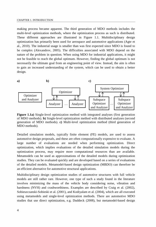
CHAPTER 1. INTRODUCTION making process became apparent. The third generation of MDO methods includes the multi-level optimization methods, where the optimization process as such is distributed. These different approaches are illustrated in Figure 1.1. Multidisciplinary design optimization has primarily been used for aerospace and automotive applications (Agte et al., 2010). The industrial usage is smaller than was first expected since MDO is found to be complex (Alexandrov, 2005). The difficulties associated with MDO depend on the nature of the problem in question. When using MDO for industrial applications, it might not be feasible to reach the global optimum. However, finding the global optimum is not necessarily the ultimate goal from an engineering point of view. Instead, the aim is often to gain an increased understanding of the system, which can be used to obtain a better design.
a) b) c)
Figure 1.1a) Single-level optimization method with integrated analyses (first generation of MDO methods). b) Single-level optimization method with distributed analyses (second generation of MDO methods). c) Multi-level optimization method (third generation of MDO methods).
Detailed simulation models, typically finite element (FE) models, are used to assess automotive design proposals, and these are often computationally expensive to evaluate. A large number of evaluations are needed when performing optimization. Direct optimization, which implies evaluations of the detailed simulation models during the optimization process, may require more computational resources than are available. Metamodels can be used as approximations of the detailed models during optimization studies. They can be evaluated quickly and are developed based on a series of evaluations of the detailed models. Metamodel-based design optimization (MBDO) can therefore be an efficient alternative for automotive structural applications.
Multidisciplinary design optimization studies of automotive structures with full vehicle models are still rather rare. However, one type of such a study found in the literature involves minimizing the mass of the vehicle body considering noise, vibration and harshness (NVH) and crashworthiness. Examples are described by Craig et al. (2002), Sobieszczanski-Sobieski et al. (2001), and Kodiyalam et al. (2004), which are all executed using metamodels and single-level optimization methods. There are automotive MDO studies that use direct optimization, e.g. Duddeck (2008), but metamodel-based design
Optimizerand Analyzer
…
Optimizer
Analyzer Analyzer …
System Optimizer
Subspace Optimizer
and Analyzer
Subspace Optimizer
and Analyzer
4
CHAPTER 1. INTRODUCTION optimization is the most common approach when computationally expensive simulation models are involved. Multi-level optimization methods are rarely used for automotive applications.
The aim of this research is to find suitable methods for large-scale MDO of automotive structures involving computationally expensive simulation models. The work has been performed within the ProOpt project, which has the goal to develop methods for optimization-driven design.
The first part of the thesis contains theory and background, and it is organized as follows. First, some basic optimization concepts are covered. Next, the nature of MDO problems is discussed, specifically focusing on automotive structural applications. Motivated by the need for metamodels when performing MDO of automotive structures, MBDO is thereafter given special attention. A number of commonly used MDO methods are then accounted for. This part of the thesis is summed up in a discussion concerning suitable ways of performing metamodel-based MDO of automotive structures. Finally, conclusions are drawn and the two appended papers are reviewed.
5

CHAPTER 1. INTRODUCTION
6
Optimization Concepts 2
Some basic optimization concepts are introduced in this chapter. First, a general optimization problem is defined. Next, structural optimization is given special attention as the focus of this thesis is to find MDO methods suitable for automotive structural applications. Finally, a short discussion concerning optimization algorithms is provided.
2.1 Optimization Problem
A general optimization problem can be formulated as
min𝐱
𝑓(𝐱)
(2.1) subject to 𝐠(𝐱) ≤ 𝟎𝐡(𝐱) = 𝟎𝐱lower ≤ 𝐱 ≤ 𝐱upper.
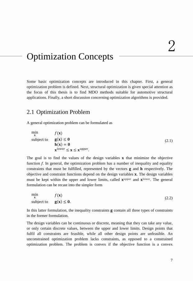
The goal is to find the values of the design variables x that minimize the objective function f. In general, the optimization problem has a number of inequality and equality constraints that must be fulfilled, represented by the vectors g and h respectively. The objective and constraint functions depend on the design variables x. The design variables must be kept within the upper and lower limits, called xupper and xlower. The general formulation can be recast into the simpler form
min𝐱
𝑓(𝐱) (2.2)
subject to 𝐠(𝐱) ≤ 𝟎.
In this latter formulation, the inequality constraints g contain all three types of constraints in the former formulation.
The design variables can be continuous or discrete, meaning that they can take any value, or only certain discrete values, between the upper and lower limits. Design points that fulfil all constraints are feasible, while all other design points are unfeasible. An unconstrained optimization problem lacks constraints, as opposed to a constrained optimization problem. The problem is convex if the objective function is a convex
7
CHAPTER 2. OPTIMIZATION CONCEPTS function and the feasible region, defined by the constraints, is a convex set. The solution of an optimization problem is called the global optimum. In a non-convex optimization problem, a number of local optima different from the global optimum may exist, while the only optimum in a convex optimization problem is the global one.
2.2 Structural Optimization
A structure is a body, or an assemblage of bodies, that can support loads. The following definition of structural optimization is provided by Gallagher (1973, p. 7): “Structural optimization seeks the selection of design variables to achieve, within the limits (constraints) placed on the structural behaviour, geometry, or other factors, its goal of optimality defined by the objective function for specified loading or environmental conditions.” Three types of structural optimization can be distinguished: size, shape, and topology optimization (Bendsøe and Sigmund, 2003). In size optimization, the design variables represent structural properties, e.g. sheet thicknesses or material parameters. In shape optimization on the other hand, the design variables represent the shape of material boundaries. Topology optimization is the most general form of structural optimization and is used to find where material should be placed to be most effective. A typical automotive structural optimization problem is a size optimization problem with sheet thicknesses and material parameters as design variables, the mass as objective function, and a number of performance measures as constraints.
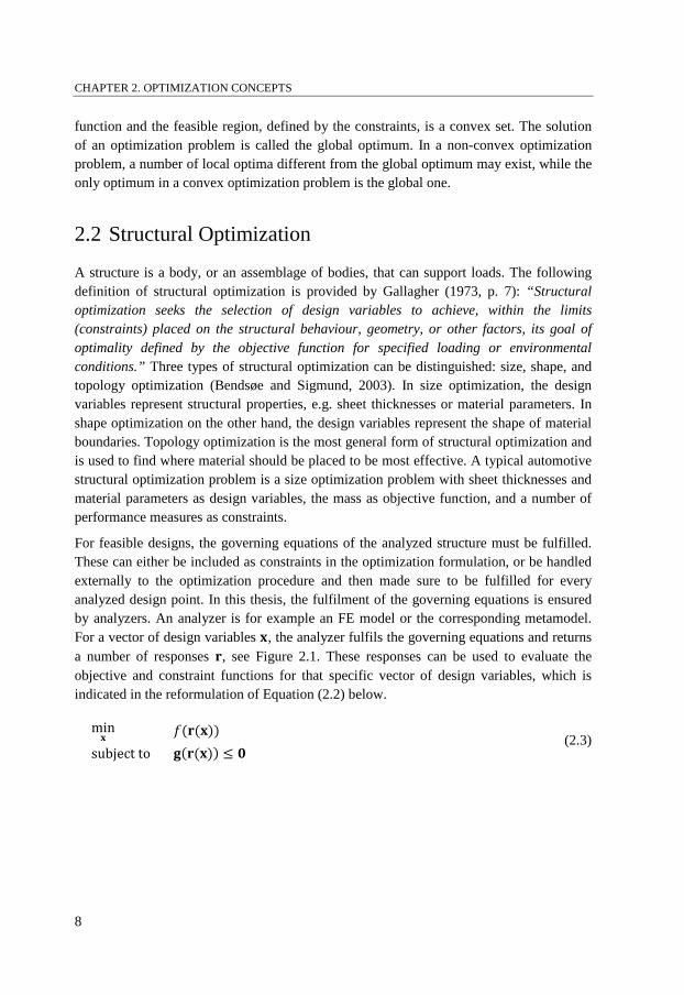
For feasible designs, the governing equations of the analyzed structure must be fulfilled. These can either be included as constraints in the optimization formulation, or be handled externally to the optimization procedure and then made sure to be fulfilled for every analyzed design point. In this thesis, the fulfilment of the governing equations is ensured by analyzers. An analyzer is for example an FE model or the corresponding metamodel. For a vector of design variables x, the analyzer fulfils the governing equations and returns a number of responses r, see Figure 2.1. These responses can be used to evaluate the objective and constraint functions for that specific vector of design variables, which is indicated in the reformulation of Equation (2.2) below.
min𝐱
𝑓(𝐫(𝐱)) (2.3)
subject to 𝐠(𝐫(𝐱)) ≤ 𝟎
8
CHAPTER 2. OPTIMIZATION CONCEPTS
Figure 2.1 Illustration of an analyzer that fulfils the governing equations.
2.3 Optimization Algorithms
Optimization problems can be solved using optimization algorithms consisting of iterative search processes. Various types of algorithms are available, and which type is suitable depends on the nature of the problem at hand. A way of classifying optimization algorithms refers to the kind of gradient information used. Zero-order algorithms only use objective and constraint function values, while first-order and second-order algorithms also use first-order and second-order gradients, respectively, and are collectively referred to as gradient-based algorithms.
One type of zero-order optimization algorithms is stochastic, or heuristic, algorithms. These are based on a random generation of points used for local search procedures and are typically inspired by some phenomenon from nature. Stochastic algorithms have a good chance of finding the global optimum and are well suited for discrete optimization problems, but require evaluations of a large number of design points (Venter, 2010). Examples of stochastic algorithms are evolutionary algorithms, simulated annealing, and particle swarm optimization. More information concerning stochastic optimization algorithms is given in Section 4.4.
Many gradient-based optimization algorithms use an iterative two-step procedure to reach a local optimum. Gradient information is first used to find a search direction, and a line-search is then performed to determine the step size. For non-convex problems, there is no guarantee that a local optimum also is the global one. However, an improved estimate of the global optimum can be found if several search procedures with different starting points are performed. Gradient-based optimization algorithms generally require few design point evaluations to reach a local optimum, but both function and gradient evaluations are needed. Moreover, they can exhibit difficulties solving discrete optimization problems and also be susceptible to numerical noise (Venter, 2010).
x r
Analyzer
9

CHAPTER 2. OPTIMIZATION CONCEPTS
10
Multidisciplinary Design Optimization Problems
3
Multidisciplinary design optimization is a formalized methodology used to perform optimization of a product considering several disciplines simultaneously. Giesing and Barthelemy (1998, p. 2) provide the following definition of MDO: “A methodology for the design of complex engineering systems and subsystems that coherently exploits the synergism of mutually interacting phenomena.” In general, a better design can be found when considering the interactions between different aspects of a product than when considering them as isolated entities, something which is taken advantage of when using MDO.
An MDO problem can be expressed by the general optimization formulation in Equation (2.2). The problem becomes multidisciplinary if the design variables, objective function, and constraints affect different disciplines. Within one discipline, many different loadcases can be considered. A loadcase is a specific configuration that is evaluated using an analyzer, e.g. a simulation of a crash scenario using an FE model, and will here be denoted subspace. The MDO methodology can just as well be applied to different loadcases within one single discipline, and the problem is then not truly multidisciplinary. However, the idea of finding a better solution by taking advantage of the interactions between subspaces still remains.
When solving large-scale MDO problems, some kind of problem decomposition is required. There are two main motivations for decomposing a problem according to Kodiyalam and Sobieszczanski-Sobieski (2001), namely concurrency and autonomy. Concurrency is achieved through distribution of the problem so that human and computational resources can work on the problem in parallel. Autonomy can be attained if individual groups responsible for certain parts of the problem are granted freedom to make their own design decisions and to govern methods and tools.
In this chapter, different aspects related to problem decomposition are considered. Thereafter, the nature of automotive MDO problems is discussed with focus on structural applications. Several MDO methods were developed for aerospace applications. In order to assess whether or not these methods are suitable for automotive structural applications, this chapter also contains a comparison between automotive and aerospace MDO problems.
11
CHAPTER 3. MULTIDISCIPLINARY DESIGN OPTIMIZATION PROBLEMS
3.1 Problem Decomposition
For single-level optimization methods, decomposition is achieved through distributing the analyses to subspace analyzers, enabling computational resources to be used in parallel. For multi-level optimization methods, the optimization process as such is distributed to subspace optimizers that communicate with a system optimizer, making it possible for individual groups to work on the problem concurrently and autonomously.
3.1.1 Terminology of Decomposed Systems The implications of problem decomposition and the associated terminology are presented in this section. Even if the decomposition is fundamentally different for single-level and multi-level optimization methods, a unified terminology can be used.
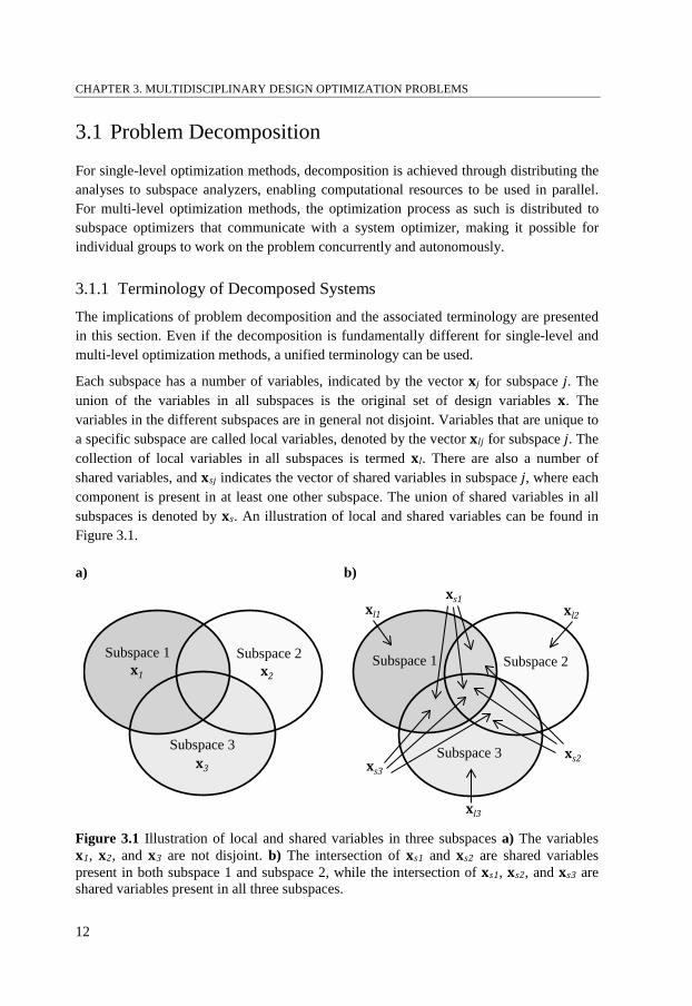
Each subspace has a number of variables, indicated by the vector xj for subspace j. The union of the variables in all subspaces is the original set of design variables x. The variables in the different subspaces are in general not disjoint. Variables that are unique to a specific subspace are called local variables, denoted by the vector xlj for subspace j. The collection of local variables in all subspaces is termed xl. There are also a number of shared variables, and xsj indicates the vector of shared variables in subspace j, where each component is present in at least one other subspace. The union of shared variables in all subspaces is denoted by xs. An illustration of local and shared variables can be found in Figure 3.1.
a) b)
Figure 3.1 Illustration of local and shared variables in three subspaces a) The variables x1, x2, and x3 are not disjoint. b) The intersection of xs1 and xs2 are shared variables present in both subspace 1 and subspace 2, while the intersection of xs1, xs2, and xs3 are shared variables present in all three subspaces.
x1 x2
x3
Subspace 1 Subspace 2
Subspace 3
xs1xl1 xl2
xl3
xs2xs3
Subspace 1 Subspace 2
Subspace 3
12
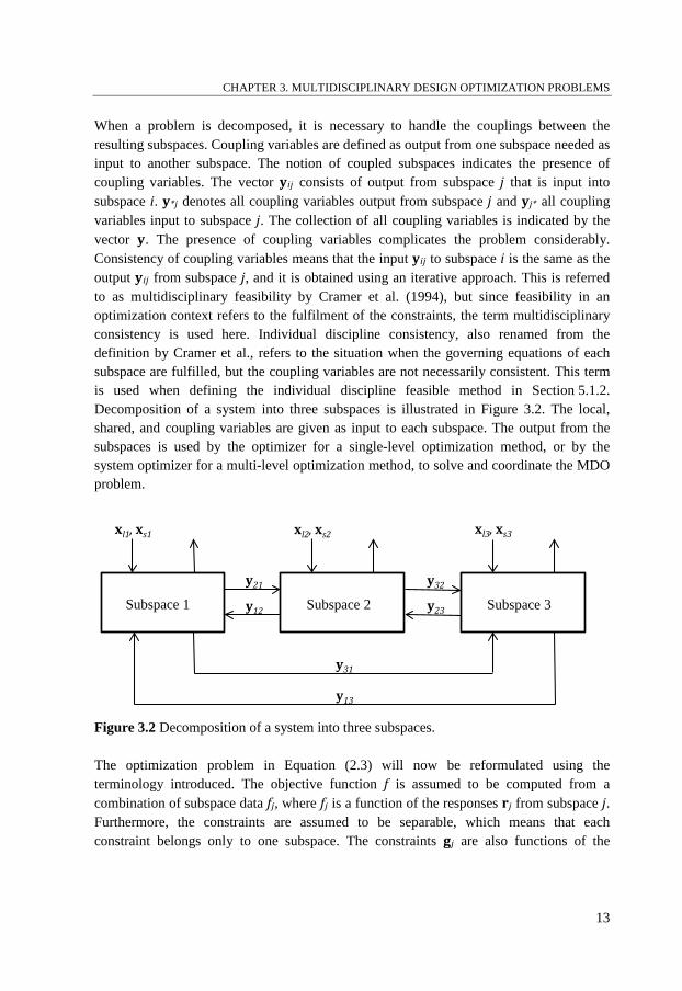
CHAPTER 3. MULTIDISCIPLINARY DESIGN OPTIMIZATION PROBLEMS When a problem is decomposed, it is necessary to handle the couplings between the resulting subspaces. Coupling variables are defined as output from one subspace needed as input to another subspace. The notion of coupled subspaces indicates the presence of coupling variables. The vector yij consists of output from subspace j that is input into subspace i. y*j denotes all coupling variables output from subspace j and yj* all coupling variables input to subspace j. The collection of all coupling variables is indicated by the vector y. The presence of coupling variables complicates the problem considerably. Consistency of coupling variables means that the input yij to subspace i is the same as the output yij from subspace j, and it is obtained using an iterative approach. This is referred to as multidisciplinary feasibility by Cramer et al. (1994), but since feasibility in an optimization context refers to the fulfilment of the constraints, the term multidisciplinary consistency is used here. Individual discipline consistency, also renamed from the definition by Cramer et al., refers to the situation when the governing equations of each subspace are fulfilled, but the coupling variables are not necessarily consistent. This term is used when defining the individual discipline feasible method in Section 5.1.2. Decomposition of a system into three subspaces is illustrated in Figure 3.2. The local, shared, and coupling variables are given as input to each subspace. The output from the subspaces is used by the optimizer for a single-level optimization method, or by the system optimizer for a multi-level optimization method, to solve and coordinate the MDO problem.
Figure 3.2 Decomposition of a system into three subspaces.
The optimization problem in Equation (2.3) will now be reformulated using the terminology introduced. The objective function f is assumed to be computed from a combination of subspace data fj, where fj is a function of the responses rj from subspace j. Furthermore, the constraints are assumed to be separable, which means that each constraint belongs only to one subspace. The constraints gj are also functions of the
xl1, xs1
Subspace 1
y13
y31
xl2, xs2
Subspace 2
xl3, xs3
Subspace 3
y21
y12
y32
y23
13
CHAPTER 3. MULTIDISCIPLINARY DESIGN OPTIMIZATION PROBLEMS responses rj from subspace j. These assumptions hold throughout this thesis. The resulting optimization formulation is then
min𝐱
𝑓(𝑓1(𝐫1(𝐱𝑙1,𝐱𝑠1, 𝐲1∗)),𝑓2(𝐫2(𝐱𝑙2, 𝐱𝑠2, 𝐲2∗)), … , 𝑓𝑛(𝐫𝑛(𝐱𝑙𝑛,𝐱𝑠𝑛, 𝐲𝑛∗))) (3.1)
subject to 𝐠𝑗�𝐫𝑗(𝐱𝑙𝑗, 𝐱𝑠𝑗, 𝐲𝑗∗)� ≤ 𝟎, 𝑗 = 1,2, … ,𝑛,
where n is the number of subspaces.
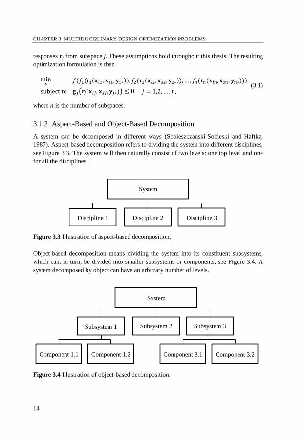
3.1.2 Aspect-Based and Object-Based Decomposition A system can be decomposed in different ways (Sobieszczanski-Sobieski and Haftka, 1987). Aspect-based decomposition refers to dividing the system into different disciplines, see Figure 3.3. The system will then naturally consist of two levels: one top level and one for all the disciplines.
Figure 3.3 Illustration of aspect-based decomposition.
Object-based decomposition means dividing the system into its constituent subsystems, which can, in turn, be divided into smaller subsystems or components, see Figure 3.4. A system decomposed by object can have an arbitrary number of levels.
Figure 3.4 Illustration of object-based decomposition.
System
Discipline 1 Discipline 3Discipline 2
System
Subsystem 1 Subsystem 3Subsystem 2
Component 1.1 Component 1.2 Component 3.1 Component 3.2
14
CHAPTER 3. MULTIDISCIPLINARY DESIGN OPTIMIZATION PROBLEMS
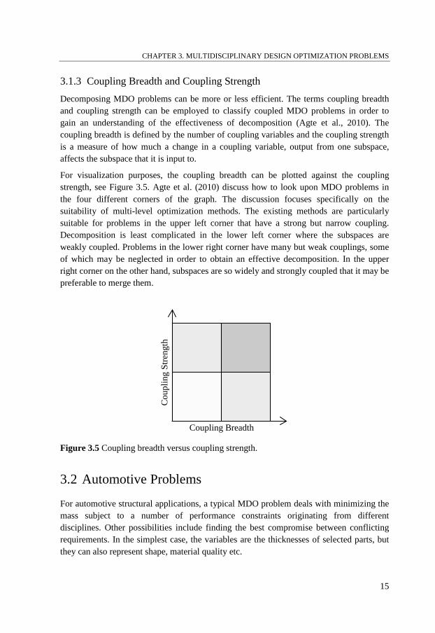
3.1.3 Coupling Breadth and Coupling Strength Decomposing MDO problems can be more or less efficient. The terms coupling breadth and coupling strength can be employed to classify coupled MDO problems in order to gain an understanding of the effectiveness of decomposition (Agte et al., 2010). The coupling breadth is defined by the number of coupling variables and the coupling strength is a measure of how much a change in a coupling variable, output from one subspace, affects the subspace that it is input to.
For visualization purposes, the coupling breadth can be plotted against the coupling strength, see Figure 3.5. Agte et al. (2010) discuss how to look upon MDO problems in the four different corners of the graph. The discussion focuses specifically on the suitability of multi-level optimization methods. The existing methods are particularly suitable for problems in the upper left corner that have a strong but narrow coupling. Decomposition is least complicated in the lower left corner where the subspaces are weakly coupled. Problems in the lower right corner have many but weak couplings, some of which may be neglected in order to obtain an effective decomposition. In the upper right corner on the other hand, subspaces are so widely and strongly coupled that it may be preferable to merge them.
Figure 3.5 Coupling breadth versus coupling strength.
3.2 Automotive Problems
For automotive structural applications, a typical MDO problem deals with minimizing the mass subject to a number of performance constraints originating from different disciplines. Other possibilities include finding the best compromise between conflicting requirements. In the simplest case, the variables are the thicknesses of selected parts, but they can also represent shape, material quality etc.
Cou
plin
g St
reng
th
Coupling Breadth
15
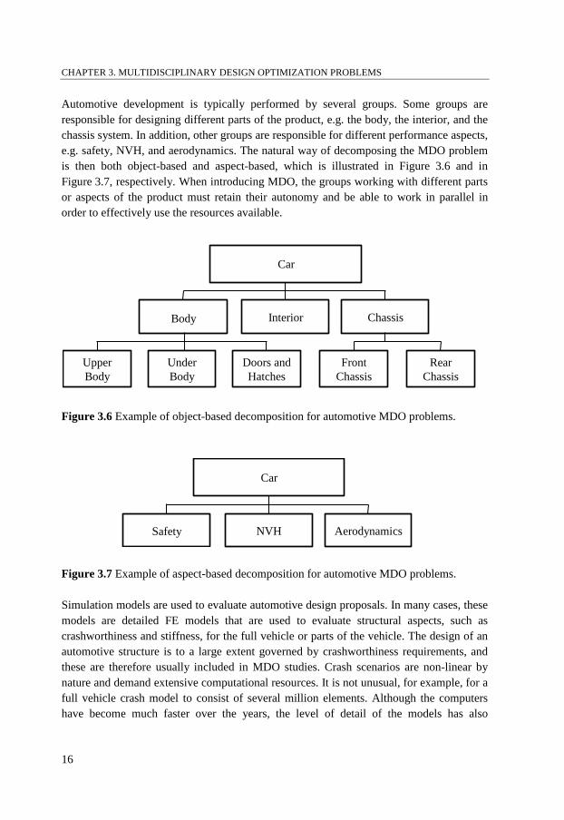
CHAPTER 3. MULTIDISCIPLINARY DESIGN OPTIMIZATION PROBLEMS Automotive development is typically performed by several groups. Some groups are responsible for designing different parts of the product, e.g. the body, the interior, and the chassis system. In addition, other groups are responsible for different performance aspects, e.g. safety, NVH, and aerodynamics. The natural way of decomposing the MDO problem is then both object-based and aspect-based, which is illustrated in Figure 3.6 and in Figure 3.7, respectively. When introducing MDO, the groups working with different parts or aspects of the product must retain their autonomy and be able to work in parallel in order to effectively use the resources available.
Figure 3.6 Example of object-based decomposition for automotive MDO problems.
Figure 3.7 Example of aspect-based decomposition for automotive MDO problems.
Simulation models are used to evaluate automotive design proposals. In many cases, these models are detailed FE models that are used to evaluate structural aspects, such as crashworthiness and stiffness, for the full vehicle or parts of the vehicle. The design of an automotive structure is to a large extent governed by crashworthiness requirements, and these are therefore usually included in MDO studies. Crash scenarios are non-linear by nature and demand extensive computational resources. It is not unusual, for example, for a full vehicle crash model to consist of several million elements. Although the computers have become much faster over the years, the level of detail of the models has also
Car
Body ChassisInterior
UpperBody
UnderBody
Doors and Hatches
Front Chassis
RearChassis
Car
Safety AerodynamicsNVH
16
CHAPTER 3. MULTIDISCIPLINARY DESIGN OPTIMIZATION PROBLEMS increased. A crashworthiness simulation therefore still takes many hours to run, even on a high-performance computing cluster. When performing optimization studies, the values of the objective and constraint functions need to be evaluated for a large number of design variable settings. Metamodel-based design optimization can be an efficient approach since it generally requires fewer evaluations of the detailed simulation models than direct optimization. The use of metamodels then becomes an inexpensive way to evaluate different design variable settings during the optimization procedure. In addition to being computationally expensive, non-linear simulation models produce complex responses resulting in optimization problems with several local optima. Moreover, gradient information may be unavailable or spurious. Stochastic optimization algorithms are then suitable when searching for the global optimum. These algorithms do not use gradients but require many evaluations in order to find the optimum, and the need for metamodels therefore becomes even more obvious. A positive spin-off of using metamodels is that they can serve as a filter for the numerically noisy responses that are typical for crash scenarios.
The automotive subspaces are typically linked by shared variables, but there are not necessarily coupling variables to be taken into account. Agte et al. (2010) state that automotive designs are created in a multi-attribute environment rather than in a truly multidisciplinary environment, and that aspects, such as NVH and crashworthiness, are coupled only by shared variables. This observation is confirmed by the weight optimization studies mentioned in the introduction. There are examples of coupled automotive disciplines, but they do not govern the development of automotive structures. The absence of coupling variables simplifies the solution process of an MDO problem considerably. In addition, it is easier to incorporate metamodels in the optimization procedure when coupling variables are not considered.
3.3 Comparison between Automotive and Aerospace Problems
There are many similarities between automotive and aerospace MDO problems. Both the automotive and aerospace industries design complex products which require the joint effort of many skilled people with expert knowledge from many different areas of the organization. The need for individual groups to work concurrently and autonomously is therefore obvious for both types of applications. However, there are also some key differences that become important when dealing with MDO.
Most aeroplane structures are dimensioned for the loads applied during everyday use multiplied by a safety factor, and there is a strong focus on fatigue. Although there is considerable movement of the wings during flight, the stresses are maintained within the elastic region. The structural analyses are therefore linear and associated with relatively
17
CHAPTER 3. MULTIDISCIPLINARY DESIGN OPTIMIZATION PROBLEMS low computational costs. The aerodynamic properties are fundamental when developing aeroplanes. Aerodynamic analyses are non-linear and computationally costly. However, in general, the analyses consider stationary states and the responses are usually smooth. Usable gradients can therefore be obtained without difficulty. The use of gradient-based optimization algorithms, which typically require fewer evaluations than stochastic optimization algorithms, is therefore a natural approach. Even though aerodynamic analyses are expensive, direct optimization may be affordable when using gradient-based algorithms. The need for metamodel-based design optimization is therefore not as obvious for aerospace applications as it is for automotive applications.
Another difference between automotive and aerospace problems is the connection between the disciplines. Aerospace problems are in general linked by both shared and coupling variables. An example of aerospace coupling variables can be found when considering the structural and aerodynamic disciplines. The slender shapes of aeroplane wings result in structural deformations induced by the aerodynamic forces. These deformations in turn affect the aerodynamics of the structure and hence the aerodynamic forces. The structural and aerodynamic disciplines are thus coupled. The same strong coupling is found neither for the corresponding automotive disciplines, nor for other disciplines typically involved when performing optimization of automotive structures. It should be easier to incorporate MDO into automotive development than into aerospace development, since less complex methods can be used when coupling variables are not considered.
18
Metamodel-Based Design Optimization
4
Metamodels are approximations of detailed simulation models that can be evaluated quickly. Metamodel-based design optimization implies using metamodels during the optimization process, and is particularly useful when the simulation models are time-consuming to evaluate. Descriptions of MBDO can be found in Simpson et al. (2001), Wang and Shan (2007), and Ryberg et al (2012), among others. Many concepts within the field of MBDO originate from response surface methodology (RSM), where polynomial metamodels, called response surfaces, are used to predict the responses from physical experiments between the experimental points (Myers et al., 2008).
A metamodel is an analytical function that approximates how a certain response from a detailed simulation model depends on a number of design variables. It is created based on a series of evaluations of the detailed model. The design of experiments (DOE) determines the design variable settings for which these evaluations are performed. The number of evaluations needed depends on the number of variables, and variable screening can be used to exclude unimportant variables in order to reduce the computational cost. Metamodels can be either local or global. A local metamodel is often a low-order polynomial and approximates the detailed model in a limited part of the design space. It is typically used when creating the metamodel and performing the optimization iteratively. A global metamodel is more complex, captures the behaviour of the detailed model in the complete design space, and can be used to perform the optimization in a single iteration. In MBDO, the metamodels, represented by the vector 𝐫�, are used during the optimization process as approximations of the responses r from the detailed simulation models. The general structural optimization problem defined in Equation (2.3) can then be reformulated according to
min𝐱
𝑓(𝐫�(𝐱)) (4.1)
subject to 𝐠(𝐫�(𝐱)) ≤ 𝟎.
Metamodels are always associated with errors, i.e. 𝐫� is not a perfect representation of r, and these can be assessed using various error measures. An illustration of creating the DOE, building the metamodel, and performing the optimization can be found in Figure 4.1.
19
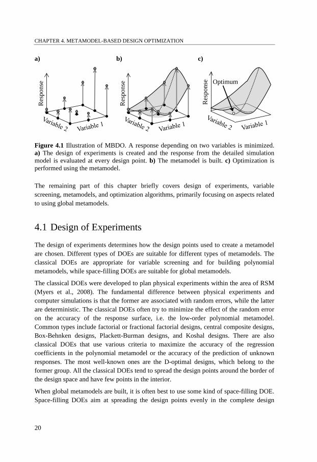
CHAPTER 4. METAMODEL-BASED DESIGN OPTIMIZATION a) b) c)
Figure 4.1 Illustration of MBDO. A response depending on two variables is minimized. a) The design of experiments is created and the response from the detailed simulation model is evaluated at every design point. b) The metamodel is built. c) Optimization is performed using the metamodel.
The remaining part of this chapter briefly covers design of experiments, variable screening, metamodels, and optimization algorithms, primarily focusing on aspects related to using global metamodels.
4.1 Design of Experiments
The design of experiments determines how the design points used to create a metamodel are chosen. Different types of DOEs are suitable for different types of metamodels. The classical DOEs are appropriate for variable screening and for building polynomial metamodels, while space-filling DOEs are suitable for global metamodels.
The classical DOEs were developed to plan physical experiments within the area of RSM (Myers et al., 2008). The fundamental difference between physical experiments and computer simulations is that the former are associated with random errors, while the latter are deterministic. The classical DOEs often try to minimize the effect of the random error on the accuracy of the response surface, i.e. the low-order polynomial metamodel. Common types include factorial or fractional factorial designs, central composite designs, Box-Behnken designs, Plackett-Burman designs, and Koshal designs. There are also classical DOEs that use various criteria to maximize the accuracy of the regression coefficients in the polynomial metamodel or the accuracy of the prediction of unknown responses. The most well-known ones are the D-optimal designs, which belong to the former group. All the classical DOEs tend to spread the design points around the border of the design space and have few points in the interior.
When global metamodels are built, it is often best to use some kind of space-filling DOE. Space-filling DOEs aim at spreading the design points evenly in the complete design
Res
pons
e
Res
pons
e Optimum
Res
pons
e
20
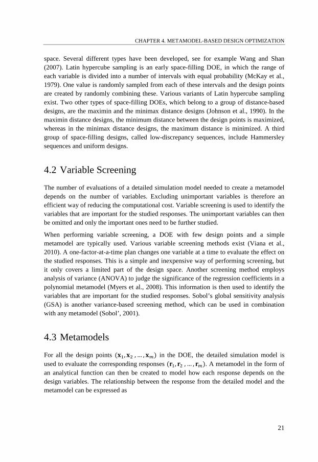
CHAPTER 4. METAMODEL-BASED DESIGN OPTIMIZATION space. Several different types have been developed, see for example Wang and Shan (2007). Latin hypercube sampling is an early space-filling DOE, in which the range of each variable is divided into a number of intervals with equal probability (McKay et al., 1979). One value is randomly sampled from each of these intervals and the design points are created by randomly combining these. Various variants of Latin hypercube sampling exist. Two other types of space-filling DOEs, which belong to a group of distance-based designs, are the maximin and the minimax distance designs (Johnson et al., 1990). In the maximin distance designs, the minimum distance between the design points is maximized, whereas in the minimax distance designs, the maximum distance is minimized. A third group of space-filling designs, called low-discrepancy sequences, include Hammersley sequences and uniform designs.
4.2 Variable Screening
The number of evaluations of a detailed simulation model needed to create a metamodel depends on the number of variables. Excluding unimportant variables is therefore an efficient way of reducing the computational cost. Variable screening is used to identify the variables that are important for the studied responses. The unimportant variables can then be omitted and only the important ones need to be further studied.
When performing variable screening, a DOE with few design points and a simple metamodel are typically used. Various variable screening methods exist (Viana et al., 2010). A one-factor-at-a-time plan changes one variable at a time to evaluate the effect on the studied responses. This is a simple and inexpensive way of performing screening, but it only covers a limited part of the design space. Another screening method employs analysis of variance (ANOVA) to judge the significance of the regression coefficients in a polynomial metamodel (Myers et al., 2008). This information is then used to identify the variables that are important for the studied responses. Sobol’s global sensitivity analysis (GSA) is another variance-based screening method, which can be used in combination with any metamodel (Sobol’, 2001).
4.3 Metamodels
For all the design points (𝐱1,𝐱2 , … , 𝐱𝑚) in the DOE, the detailed simulation model is used to evaluate the corresponding responses (𝐫1, 𝐫2 , … , 𝐫𝑚). A metamodel in the form of an analytical function can then be created to model how each response depends on the design variables. The relationship between the response from the detailed model and the metamodel can be expressed as
21
CHAPTER 4. METAMODEL-BASED DESIGN OPTIMIZATION
𝑟(𝐱) = �̂�(𝐱) + 𝜀, (4.2)
where r is the response from the detailed simulation model, �̂� is the corresponding metamodel, and ε is the metamodel error. A metamodel can either interpolate or approximate the response from the detailed model, depending on the formulation. Interpolating metamodels are not necessarily better than approximating ones at predicting the response between the simulated design points.
Various types of metamodels can be found in the literature, see e.g. Simpson et al. (2001) and Ryberg et al. (2012). Polynomial metamodels can be constructed using linear regression, and these are often used to perform variable screening or to model responses locally in the design space (Myers et al., 2008). Examples of global metamodels include Kriging, artificial neural networks, radial basis functions, multivariate adaptive regression splines, and support vector regression. Focus will here be put on radial basis function neural networks and feedforward neural networks, two types of artificial neural networks.
4.3.1 Artificial Neural Networks Artificial neural networks (ANNs), often simply called neural networks, are inspired by the biological nervous system. They are composed of neurons assembled into architectures. Each neuron performs a biased weighted sum of their inputs and uses a transfer function to generate the output. The connection topology of the neurons and the transfer function used in the neurons determine the type of neural network. An ANN must be trained using data from the detailed simulations. The training process involves finding the weights and biases that minimize some kind of error measure. Neural networks are described by Bishop (1995), among others.
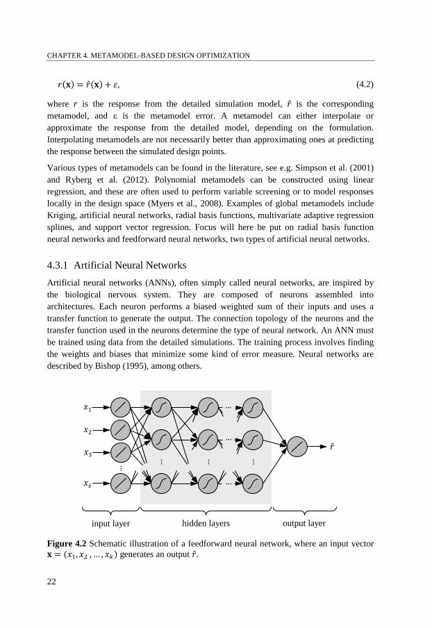
Figure 4.2 Schematic illustration of a feedforward neural network, where an input vector 𝐱 = (𝑥1, 𝑥2 , … , 𝑥𝑘) generates an output �̂�.
𝑥1
𝑥2
𝑥k
…
𝑥3
… … …
…
…
…
hidden layersinput layer output layer
22
CHAPTER 4. METAMODEL-BASED DESIGN OPTIMIZATION In a feedforward neural network (FFNN), information is only passed forward. There is one input layer, one or several hidden layers, and one output layer. Each layer consists of a number of neurons. The neurons in the hidden layers typically have sigmoid transfer functions, while the neurons in the input and output layers have linear transfer functions. An illustration of an FFNN can be found in Figure 4.2. Another type of neural network is the radial basis function neural network (RBFNN). In contrast to FFNN, it only has one hidden layer and the transfer functions in this layer are radial basis functions. Radial basis functions can be of different kinds, but Gaussian transfer functions are often used.
4.3.2 Metamodel Validation There are several ways of assessing the accuracy of a metamodel, see e.g. Stander et al. (2012). Fitting errors give information about how well the metamodel is fitted to the data obtained from the detailed simulation model. These are typically based on the residuals, i.e. the difference between the values obtained from the detailed model (𝑟1, 𝑟2 , … , 𝑟𝑚) and the metamodel (�̂�1, �̂�2 , … , �̂�𝑚). Small residuals imply a more accurate reflection of the dataset than large residuals. The root mean squared error (RMSE) can be expressed as
RMSE = �1𝑚�(𝑟𝑖 − �̂�𝑖)2𝑚
𝑖=1
, (4.3)
where m is the number of data points. Another commonly used fitting error is the coefficient of determination, R2, which measures how well the metamodel captures the variability in the dataset.
𝑅2 =∑ (�̂�𝑖 − �̅�)2𝑚𝑖=1
∑ (𝑟𝑖 − �̅�)2𝑚𝑖=1
, (4.4)
where �̅� is the mean response from the detailed model. R2 can have values between 0 and 1, and a value of 1 indicates a perfect fit. Fitting errors are irrelevant for interpolating metamodels, which always fit perfectly to the dataset.
Prediction errors give information about the ability of the metamodel to predict the responses in unknown points. These errors can be assessed by using a different dataset for validation than for fitting the metamodel. The same type of error measures used for estimating fitting errors can then be used for prediction errors, e.g. RMSE. However, to use a dataset only for validation can often not be afforded in practical situations. A useful way of estimating the predicting capabilities of a metamodel without having to create a separate validation set is to use cross validation (CV). In leave-one-out CV, a metamodel is fitted to all data points but one, and an error measure is evaluated at the omitted point. This process is repeated until all points have been omitted and the obtained error measures
23
CHAPTER 4. METAMODEL-BASED DESIGN OPTIMIZATION are combined into one value. Using RMSE, the leave-one-out CV error can be expressed as
RMSECV = �1𝑚��𝑟𝑖 − �̂�𝑖
(−𝑖)�2
𝑚
𝑖=1
, (4.5)
where �̂�𝑖(−𝑖) is obtained from the metamodel created without the ith point. Note that the
complete dataset is used for the final metamodel.
Finally, it is worth noting that one single error measure never can give the complete picture of the accuracy of a metamodel, and it is therefore important to always use several error measures.
4.4 Stochastic Optimization Algorithms
Stochastic optimization algorithms are particularly suitable for MBDO involving complex responses resulting in optimization problems with several local optima. These types of algorithms have a good chance of finding the global optimum using a large number of function evaluations, which can be afforded since the evaluations of metamodels are quick. Examples of stochastic optimization algorithms are genetic algorithms, evolution strategies, particle swarm optimization, and simulated annealing. The following discussion is restricted to evolutionary algorithms, which include genetic algorithms and evolution strategies, and to simulated annealing.
4.4.1 Evolutionary Algorithms Evolutionary algorithms (ESs) use mechanisms inspired by biological evolution to search for the global optimum. The principal idea is that natural selection increases the fitness of a population of individuals. An individual is a design point and the fitness is represented by the objective function, which can be penalized by constraint violations. Two common types of EAs are genetic algorithms and evolution strategies.
Evolutionary algorithms go through a number of evolution cycles, see Figure 4.3 (Eiben and Smith, 2003). The population is first initiated by randomly creating a number of individuals. Based on the fitness of these individuals, the parents for the next generation are chosen. This process is generally stochastic, meaning that individuals with high fitness have a high probability of being selected and vice versa. A number of children are generated from the parents using recombination or mutation, or both. Recombination typically implies combining two parents into one or two children, and mutation means that a parent results in a slightly modified child. Both recombination and mutation are
24
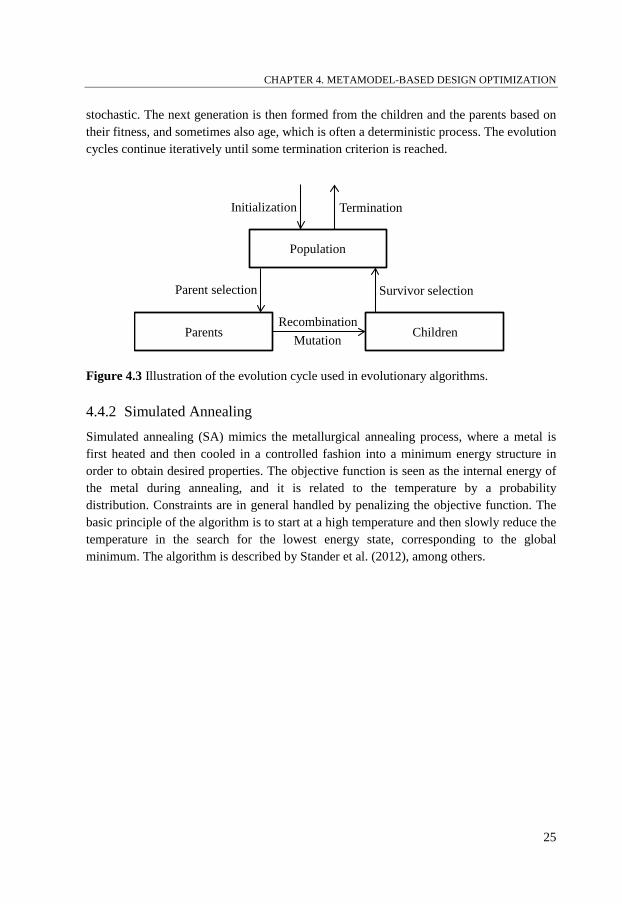
CHAPTER 4. METAMODEL-BASED DESIGN OPTIMIZATION stochastic. The next generation is then formed from the children and the parents based on their fitness, and sometimes also age, which is often a deterministic process. The evolution cycles continue iteratively until some termination criterion is reached.
Figure 4.3 Illustration of the evolution cycle used in evolutionary algorithms.
4.4.2 Simulated Annealing Simulated annealing (SA) mimics the metallurgical annealing process, where a metal is first heated and then cooled in a controlled fashion into a minimum energy structure in order to obtain desired properties. The objective function is seen as the internal energy of the metal during annealing, and it is related to the temperature by a probability distribution. Constraints are in general handled by penalizing the objective function. The basic principle of the algorithm is to start at a high temperature and then slowly reduce the temperature in the search for the lowest energy state, corresponding to the global minimum. The algorithm is described by Stander et al. (2012), among others.
Population
ChildrenParents
Initialization Termination
Parent selection Survivor selection
RecombinationMutation
25

CHAPTER 4. METAMODEL-BASED DESIGN OPTIMIZATION
26
Multidisciplinary Design Optimization Methods
5
Multidisciplinary design optimization methods are used to solve MDO problems. The methods can be divided into two main categories: single-level and multi-level optimization methods. Using single-level methods, the optimization process is performed by one single optimizer, while the optimization process is distributed using multi-level methods. A number of different MDO methods are documented in the literature. When choosing an MDO method for solving a specific MDO problem, the nature of the problem and the environment in which the problem is to be solved must be taken into account.
An MDO method defines aspects related to optimization formulation, coordination, and optimization algorithms. For a single-level method, the optimization formulation is defined by the single optimization problem. For a multi-level method on the other hand, the optimization formulation is defined by several optimization problems on several levels. Multi-level methods must also coordinate the optimization problems included in the formulation, i.e. specify the order in which the problems are to be solved, to make sure that the solutions of the individual problems lead to the solution of the entire problem. Finally, how to solve a specific optimization problem is defined by an optimization algorithm.
The aim of this chapter is to describe a number of commonly used MDO methods, primarily focusing on the optimization formulations. However, the issues of coordination or the implications of choosing a certain type of optimization algorithm are also discussed for some methods. The notation used to define the optimization formulations is specified in Section 3.1.1.
5.1 Single-Level Optimization Methods
Common to single-level optimization methods is a central optimizer that makes all design decisions. If the analyses are distributed, computer resources can be used in parallel, and individual groups can govern methods and tools for performing the analyses. The two methods presented here are distinguished by the kind of consistency that is maintained during the optimization process.
27
CHAPTER 5. MULTIDISCIPLINARY DESIGN OPTIMIZATION METHODS
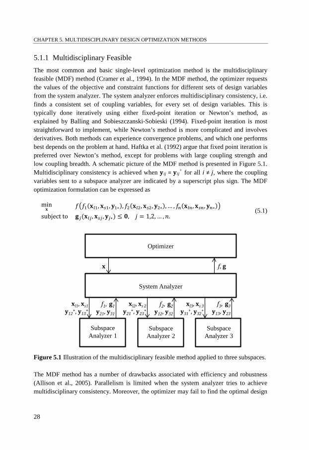
5.1.1 Multidisciplinary Feasible The most common and basic single-level optimization method is the multidisciplinary feasible (MDF) method (Cramer et al., 1994). In the MDF method, the optimizer requests the values of the objective and constraint functions for different sets of design variables from the system analyzer. The system analyzer enforces multidisciplinary consistency, i.e. finds a consistent set of coupling variables, for every set of design variables. This is typically done iteratively using either fixed-point iteration or Newton’s method, as explained by Balling and Sobieszczanski-Sobieski (1994). Fixed-point iteration is most straightforward to implement, while Newton’s method is more complicated and involves derivatives. Both methods can experience convergence problems, and which one performs best depends on the problem at hand. Haftka et al. (1992) argue that fixed point iteration is preferred over Newton’s method, except for problems with large coupling strength and low coupling breadth. A schematic picture of the MDF method is presented in Figure 5.1. Multidisciplinary consistency is achieved when yij = yij
+ for all i ≠ j, where the coupling variables sent to a subspace analyzer are indicated by a superscript plus sign. The MDF optimization formulation can be expressed as
min𝐱
𝑓�𝑓1(𝐱𝑙1, 𝐱𝑠1, 𝐲1∗),𝑓2(𝐱𝑙2,𝐱𝑠2, 𝐲2∗), … ,𝑓𝑛(𝐱𝑙𝑛, 𝐱𝑠𝑛, 𝐲𝑛∗)� (5.1) subject to 𝐠𝑗(𝐱𝑙𝑗, 𝐱𝑠𝑗 , 𝐲𝑗∗) ≤ 𝟎, 𝑗 = 1,2, … ,𝑛.
Figure 5.1 Illustration of the multidisciplinary feasible method applied to three subspaces.
The MDF method has a number of drawbacks associated with efficiency and robustness (Allison et al., 2005). Parallelism is limited when the system analyzer tries to achieve multidisciplinary consistency. Moreover, the optimizer may fail to find the optimal design
x f, g
System Analyzer
xl1, xs1 y12
+, y13+
f1, g1y21, y31
Subspace Analyzer 1
Subspace Analyzer 3
Optimizer
Subspace Analyzer 2
xl2, xs 2y21
+, y23+
f2, g2y12, y32
xl3, xs 3y31
+, y32+
f3, g3y13, y23
28
CHAPTER 5. MULTIDISCIPLINARY DESIGN OPTIMIZATION METHODS if the system analyzer has convergence problems. These shortcomings motivate the development of alternative methods.
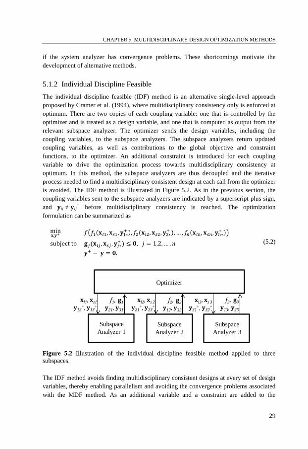
5.1.2 Individual Discipline Feasible The individual discipline feasible (IDF) method is an alternative single-level approach proposed by Cramer et al. (1994), where multidisciplinary consistency only is enforced at optimum. There are two copies of each coupling variable: one that is controlled by the optimizer and is treated as a design variable, and one that is computed as output from the relevant subspace analyzer. The optimizer sends the design variables, including the coupling variables, to the subspace analyzers. The subspace analyzers return updated coupling variables, as well as contributions to the global objective and constraint functions, to the optimizer. An additional constraint is introduced for each coupling variable to drive the optimization process towards multidisciplinary consistency at optimum. In this method, the subspace analyzers are thus decoupled and the iterative process needed to find a multidisciplinary consistent design at each call from the optimizer is avoided. The IDF method is illustrated in Figure 5.2. As in the previous section, the coupling variables sent to the subspace analyzers are indicated by a superscript plus sign, and yij ≠ yij
+ before multidisciplinary consistency is reached. The optimization formulation can be summarized as
min𝐱,𝐲+
𝑓�𝑓1(𝐱𝑙1, 𝐱𝑠1, 𝐲1∗+ ),𝑓2(𝐱𝑙2,𝐱𝑠2, 𝐲2∗+ ), … , 𝑓𝑛(𝐱𝑙𝑛, 𝐱𝑠𝑛, 𝐲𝑛∗+ )� (5.2) subject to 𝐠𝑗(𝐱𝑙𝑗, 𝐱𝑠𝑗 , 𝐲𝑗∗+ ) ≤ 𝟎,
𝐲+ − 𝐲 = 𝟎. 𝑗 = 1,2, … ,𝑛
Figure 5.2 Illustration of the individual discipline feasible method applied to three subspaces.
The IDF method avoids finding multidisciplinary consistent designs at every set of design variables, thereby enabling parallelism and avoiding the convergence problems associated with the MDF method. As an additional variable and a constraint are added to the
Optimizer
xl1, xs1 y12
+, y13+
f1, g1y21, y31
Subspace Analyzer 1
Subspace Analyzer 3
Subspace Analyzer 2
xl2, xs 2y21
+, y23+
f2, g2y12, y32
xl3, xs 3y31
+, y32+
f3, g3y13, y23
29
CHAPTER 5. MULTIDISCIPLINARY DESIGN OPTIMIZATION METHODS optimization formulation for every coupling variable, the method is most efficient for problems with low coupling breadth. Allison et al. (2005) use an example problem that allows for variable coupling strength to show that IDF is more suitable than MDF for strongly coupled problems.
5.2 Multi-Level Optimization Methods
The single-level optimization methods presented in the previous section have a central optimizer making all design decisions. Distribution of the decision-making process is enabled using multi-level optimization methods, where a system optimizer communicates with a number of subspace optimizers. Individual groups can then work on the MDO problem concurrently, and govern methods and tools for their analyses and their part of the optimization process. Several multi-level optimization methods have been presented in the literature and some of the most well-known ones are investigated in the following sections.
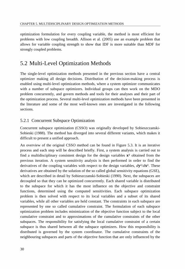
5.2.1 Concurrent Subspace Optimization Concurrent subspace optimization (CSSO) was originally developed by Sobieszczanski-Sobieski (1988). The method has diverged into several different variants, which makes it difficult to present a unified approach.
An overview of the original CSSO method can be found in Figure 5.3. It is an iterative process and each step will be described briefly. First, a system analysis is carried out to find a multidisciplinary consistent design for the design variables xk obtained from the previous iteration. A system sensitivity analysis is then performed in order to find the derivatives of the coupling variables with respect to the design variables, dyk/dxk. These derivatives are obtained by the solution of the so called global sensitivity equations (GSE), which are described in detail by Sobieszczanski-Sobieski (1990). Next, the subspaces are decoupled so that they can be optimized concurrently. Each shared variable is distributed to the subspace for which it has the most influence on the objective and constraint functions, determined using the computed sensitivities. Each subspace optimization problem is then solved with respect to its local variables and a subset of its shared variables, while all other variables are held constant. The constraints in each subspace are represented by one so called cumulative constraint. The formulation of each subspace optimization problem includes minimization of the objective function subject to the local cumulative constraint and to approximations of the cumulative constraints of the other subspaces. The responsibility for satisfying the local cumulative constraint of a certain subspace is thus shared between all the subspace optimizers. How this responsibility is distributed is governed by the system coordinator. The cumulative constraints of the neighbouring subspaces and parts of the objective function that are only influenced by the
30
CHAPTER 5. MULTIDISCIPLINARY DESIGN OPTIMIZATION METHODS subspace indirectly, are evaluated using the sensitivities computed in the previous step. The new design point xk+1 is simply the combination of optimized variables from the different subspaces. This point is not necessarily feasible, as shown by Pan and Diaz (1989). Finally, the system coordinator redistributes the responsibility for the different cumulative constraints to further reduce the objective function in the next iteration. The process will continue iteratively until convergence is reached.
Figure 5.3 Schematic picture of the original CSSO method for three subspaces.
Bloebaum et al. (1992) successfully implement the CSSO method, but incorporate some modifications to the system coordinator to achieve convergence. Pan and Diaz (1989) illustrate how a sequential solution strategy of the subspace optimizations and the combination of optimized variables can result in pseudo optimal points, i.e. points that are optimal in each subspace but that are not optimal for the full problem. They suggest a strategy to move away from pseudo-optimal points when solving the subspace optimization problems in sequence. Shankar et al. (1993) show that the original method fails solving simple quadratic problems. They propose a modified method, which is used to successfully solve large quadratic problems with weak coupling, but which does not behave well on large quadratic problems with strong coupling.
A variant of CSSO is presented by Renaud and Gabriele (1991). They use a system optimizer, instead of the system coordinator in the original version, to optimize a global approximation of the problem. The approach is summarized below and is also depicted in
System Analyzer(Including
Subspace Analyzers)
Subspace Optimizer and Analyzer 1
System CoordinatorSystem Sensitivity Analyzer
(Including SubspaceSensitivity Analyzers)
x0
xk+1
xk+1dyk / dxk
yk
xk
Subspace Optimizer and Analyzer 2
Subspace Optimizer and Analyzer 3
31
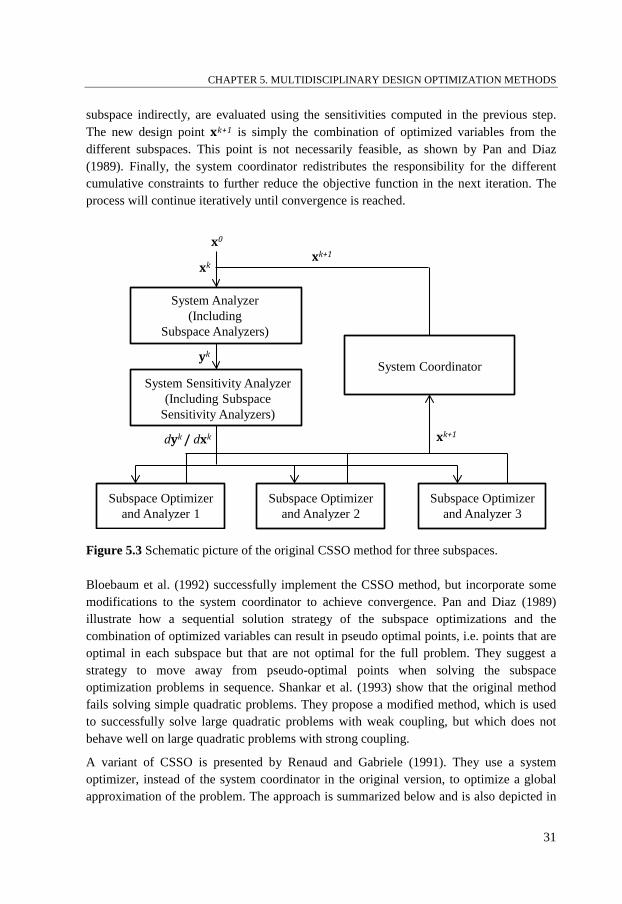
CHAPTER 5. MULTIDISCIPLINARY DESIGN OPTIMIZATION METHODS Figure 5.4. The first steps in this method are in principle the same as in the original CSSO method, including the system analysis, the system sensitivity analysis, and the concurrently performed subspace optimizations, and result in the optimized variables xk+1,sub. A design database is introduced, where information about the objective function, constraints, and associated gradients in the design points evaluated by the system and subspace analyzers are stored. The design database is used to formulate an approximation of the global problem around xk+1,sub. Optimization of the approximated global problem is then performed and the obtained optimum, xk+1, is the design vector input to the next iteration. Renaud and Gabriele (1993) develop the method by making the approximation of the global problem more accurate. In a later publication, they replace the cumulative constraints by the individual constraints (Renaud and Gabriele, 1994). Both measures yield improved convergence of the optimization process.
Figure 5.4 Illustration of the modified CSSO method presented by Renaud and Gabriele applied to three subspaces.
Starting from the modifications proposed by Renaud and Gabriele, Wujek et al. (1995) suggest further development of the CSSO method by introducing variable sharing between the subspaces and second order polynomials to approximate the global problem. Variable sharing allows variables to be allocated to more than one subspace, making the approximation of the global problem more accurate. Sellar et al. (1996) also proceed from the aforementioned modifications, but use neural networks as a global approximation of the problem. The neural networks are first used by the subspace optimizers instead of the
System Optimizer
Design Database
x0
xk+1
dyk /dxk
xk+1,sub
xk
System Analyzer(Including
Subspace Analyzers)
System Sensitivity Analyzer(Including Subspace
Sensitivity Analyzers)
yk
Subspace Optimizer and Analyzer 1
Subspace Optimizer and Analyzer 2
Subspace Optimizer and Analyzer 3
32
CHAPTER 5. MULTIDISCIPLINARY DESIGN OPTIMIZATION METHODS computed sensitivities to estimate how their design decisions affect the other subspaces, and then by the system optimizer to find a new approximate optimal design.
Distributing the responsibility of the design variables to the different subspaces, which is done in the original CSSO method, is an attractive idea. However, this method has several shortcomings. Renaud and Gabriele (1991) therefore introduce a different approach, but the variants that are based on their work suffer from the drawback that all variables are dealt with at the system level. This restricts the autonomy of the groups responsible for each subspace, which is the main motivation for using a multi-level optimization method.
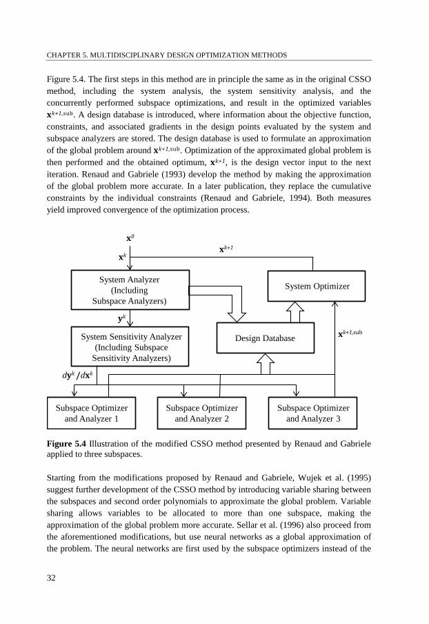
5.2.2 Bi-Level Integrated System Synthesis Bi-level integrated system synthesis (BLISS) was first introduced by Sobieszczanski-Sobieski et al. (1998). The original implementation concerned four coupled subspaces of a supersonic business jet: structures, aerodynamics, propulsion, and aircraft range. The method is iterative and optimizes the design in two main steps. First, subspace optimizations with respect to the local variables are performed in parallel. Next, the system optimizer finds the best design with respect to the shared variables.
Figure 5.5 Schematic picture of the original BLISS method applied to three subspaces.
A flowchart of the original BLISS method can be found in Figure 5.5. The first two steps are identical to the first two steps in the CSSO method described in Section 5.2.1, but are
System Analyzer(Including
Subspace Analyzers)
Subspace Optimizer and Analyzer 1
System Optimizer
System Sensitivity Analyzer(Including Subspace
Sensitivity Analyzers)
x0
xk+1= (xlk+1, xs
k+1)
xlk+1dyk / dxl
k
yk
xk
Subspace Optimizer and Analyzer 2
Subspace Optimizer and Analyzer 3
BLISS/A or BLISS/B
df /dxsk
xsk+1
33
CHAPTER 5. MULTIDISCIPLINARY DESIGN OPTIMIZATION METHODS explained in more detail here. A system analysis is first performed for the design variables obtained from the previous iteration in order to find a multidisciplinary consistent design, i.e. the coupling variables yk corresponding to the design variables xk are found for iteration k+1. This process typically includes performing subspace analyses in an iterative fashion in order to find the values of the coupling variables, and how this can be done is described in Section 5.1.1. In the second step, a sensitivity analysis is carried out in order to find the derivatives of the coupling variables with respect to the local variables, dyk/dxlk. Subspace sensitivity analyses are first performed in order to find the partial derivatives of the coupling variables output from each subspace with respect to the coupling and local variables input to that subspace. A linear equation system is then solved for each local variable in order to find the total derivatives of the coupling variables with respect to that variable. These equations are called the global sensitivity equations, see Sobieszczanski-Sobieski (1990) for more details.
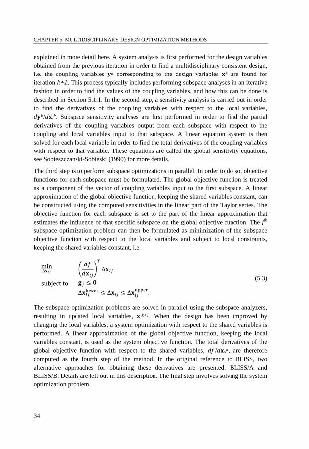
The third step is to perform subspace optimizations in parallel. In order to do so, objective functions for each subspace must be formulated. The global objective function is treated as a component of the vector of coupling variables input to the first subspace. A linear approximation of the global objective function, keeping the shared variables constant, can be constructed using the computed sensitivities in the linear part of the Taylor series. The objective function for each subspace is set to the part of the linear approximation that estimates the influence of that specific subspace on the global objective function. The jth subspace optimization problem can then be formulated as minimization of the subspace objective function with respect to the local variables and subject to local constraints, keeping the shared variables constant, i.e.
min∆𝐱𝑙𝑗
�𝑑𝑓𝑑𝐱𝑙𝑗
�𝑇
∆𝐱𝑙𝑗 (5.3)
subject to 𝐠𝑗 ≤ 𝟎∆𝐱𝑙𝑗lower ≤ ∆𝐱𝑙𝑗 ≤ ∆𝐱𝑙𝑗
upper.
The subspace optimization problems are solved in parallel using the subspace analyzers, resulting in updated local variables, xlk+1. When the design has been improved by changing the local variables, a system optimization with respect to the shared variables is performed. A linear approximation of the global objective function, keeping the local variables constant, is used as the system objective function. The total derivatives of the global objective function with respect to the shared variables, df /dxsk, are therefore computed as the fourth step of the method. In the original reference to BLISS, two alternative approaches for obtaining these derivatives are presented: BLISS/A and BLISS/B. Details are left out in this description. The final step involves solving the system optimization problem,
34
CHAPTER 5. MULTIDISCIPLINARY DESIGN OPTIMIZATION METHODS
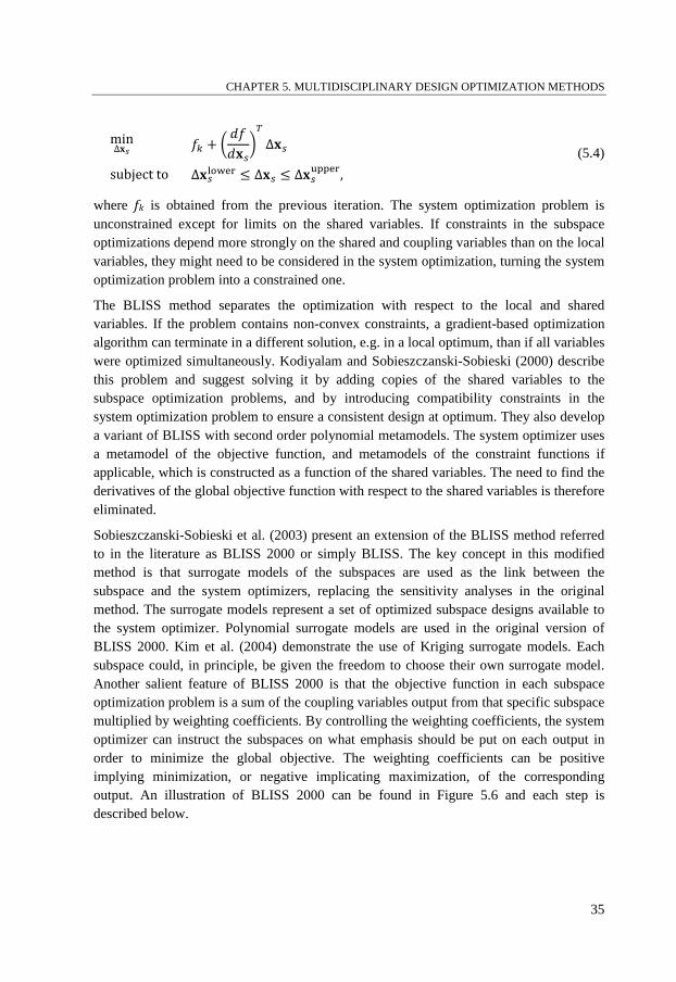
min∆𝐱𝑠
𝑓𝑘 + �𝑑𝑓𝑑𝐱𝑠
�𝑇
∆𝐱𝑠 (5.4) subject to ∆𝐱𝑠lower ≤ ∆𝐱𝑠 ≤ ∆𝐱𝑠
upper,
where fk is obtained from the previous iteration. The system optimization problem is unconstrained except for limits on the shared variables. If constraints in the subspace optimizations depend more strongly on the shared and coupling variables than on the local variables, they might need to be considered in the system optimization, turning the system optimization problem into a constrained one.
The BLISS method separates the optimization with respect to the local and shared variables. If the problem contains non-convex constraints, a gradient-based optimization algorithm can terminate in a different solution, e.g. in a local optimum, than if all variables were optimized simultaneously. Kodiyalam and Sobieszczanski-Sobieski (2000) describe this problem and suggest solving it by adding copies of the shared variables to the subspace optimization problems, and by introducing compatibility constraints in the system optimization problem to ensure a consistent design at optimum. They also develop a variant of BLISS with second order polynomial metamodels. The system optimizer uses a metamodel of the objective function, and metamodels of the constraint functions if applicable, which is constructed as a function of the shared variables. The need to find the derivatives of the global objective function with respect to the shared variables is therefore eliminated.
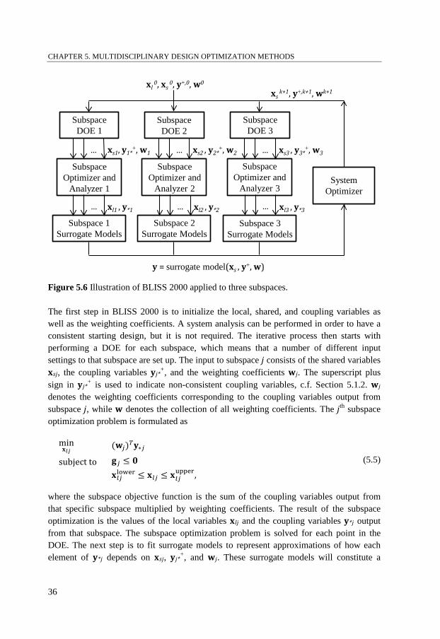
Sobieszczanski-Sobieski et al. (2003) present an extension of the BLISS method referred to in the literature as BLISS 2000 or simply BLISS. The key concept in this modified method is that surrogate models of the subspaces are used as the link between the subspace and the system optimizers, replacing the sensitivity analyses in the original method. The surrogate models represent a set of optimized subspace designs available to the system optimizer. Polynomial surrogate models are used in the original version of BLISS 2000. Kim et al. (2004) demonstrate the use of Kriging surrogate models. Each subspace could, in principle, be given the freedom to choose their own surrogate model. Another salient feature of BLISS 2000 is that the objective function in each subspace optimization problem is a sum of the coupling variables output from that specific subspace multiplied by weighting coefficients. By controlling the weighting coefficients, the system optimizer can instruct the subspaces on what emphasis should be put on each output in order to minimize the global objective. The weighting coefficients can be positive implying minimization, or negative implicating maximization, of the corresponding output. An illustration of BLISS 2000 can be found in Figure 5.6 and each step is described below.
35
CHAPTER 5. MULTIDISCIPLINARY DESIGN OPTIMIZATION METHODS
Figure 5.6 Illustration of BLISS 2000 applied to three subspaces.
The first step in BLISS 2000 is to initialize the local, shared, and coupling variables as well as the weighting coefficients. A system analysis can be performed in order to have a consistent starting design, but it is not required. The iterative process then starts with performing a DOE for each subspace, which means that a number of different input settings to that subspace are set up. The input to subspace j consists of the shared variables xsj, the coupling variables yj*
+, and the weighting coefficients wj. The superscript plus sign in yj*
+ is used to indicate non-consistent coupling variables, c.f. Section 5.1.2. wj denotes the weighting coefficients corresponding to the coupling variables output from subspace j, while w denotes the collection of all weighting coefficients. The jth subspace optimization problem is formulated as
min𝐱𝑙𝑗
(𝐰𝑗)𝑇𝐲∗𝑗 (5.5) subject to 𝐠𝑗 ≤ 𝟎
𝐱𝑙𝑗lower ≤ 𝐱𝑙𝑗 ≤ 𝐱𝑙𝑗upper,
where the subspace objective function is the sum of the coupling variables output from that specific subspace multiplied by weighting coefficients. The result of the subspace optimization is the values of the local variables xlj and the coupling variables y*j output from that subspace. The subspace optimization problem is solved for each point in the DOE. The next step is to fit surrogate models to represent approximations of how each element of y*j depends on xsj, yj*
+, and wj. These surrogate models will constitute a
System Optimizer
xl 0, xs
0, y+,0, w0
xsk+1, y+,k+1, wk+1
Subspace DOE 2
Subspace DOE 3
Subspace DOE 1
Subspace Optimizer and
Analyzer 1
Subspace Optimizer and
Analyzer 2
Subspace Optimizer and
Analyzer 3
Subspace 1 Surrogate Models
y = surrogate model(xs , y+, w)
xl1 , y*1
xs1, y1*+, w1
xl2 , y*2
xs2 , y2*+, w2
xl3 , y*3
xs3 , y3*+, w3…
…
… …
… …
Subspace 3 Surrogate Models
Subspace 2 Surrogate Models
36
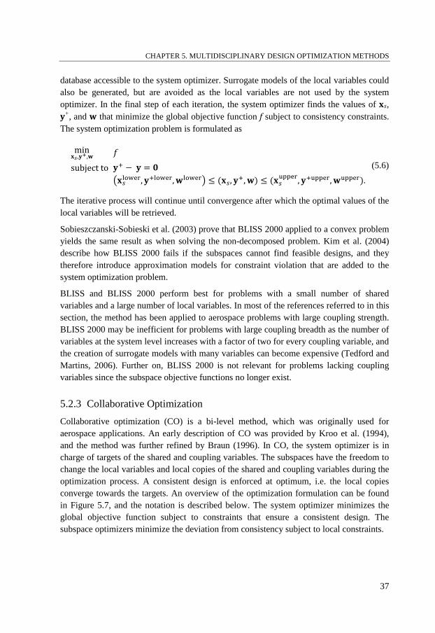
CHAPTER 5. MULTIDISCIPLINARY DESIGN OPTIMIZATION METHODS database accessible to the system optimizer. Surrogate models of the local variables could also be generated, but are avoided as the local variables are not used by the system optimizer. In the final step of each iteration, the system optimizer finds the values of xs, y+, and w that minimize the global objective function f subject to consistency constraints. The system optimization problem is formulated as
min𝐱𝑠,𝐲+,𝐰
𝑓 (5.6) subject to 𝐲+ − 𝐲 = 𝟎
�𝐱𝑠lower, 𝐲+lower,𝐰lower� ≤ (𝐱𝑠, 𝐲+,𝐰) ≤ (𝐱𝑠upper, 𝐲+upper,𝐰upper).
The iterative process will continue until convergence after which the optimal values of the local variables will be retrieved.
Sobieszczanski-Sobieski et al. (2003) prove that BLISS 2000 applied to a convex problem yields the same result as when solving the non-decomposed problem. Kim et al. (2004) describe how BLISS 2000 fails if the subspaces cannot find feasible designs, and they therefore introduce approximation models for constraint violation that are added to the system optimization problem.
BLISS and BLISS 2000 perform best for problems with a small number of shared variables and a large number of local variables. In most of the references referred to in this section, the method has been applied to aerospace problems with large coupling strength. BLISS 2000 may be inefficient for problems with large coupling breadth as the number of variables at the system level increases with a factor of two for every coupling variable, and the creation of surrogate models with many variables can become expensive (Tedford and Martins, 2006). Further on, BLISS 2000 is not relevant for problems lacking coupling variables since the subspace objective functions no longer exist.
5.2.3 Collaborative Optimization Collaborative optimization (CO) is a bi-level method, which was originally used for aerospace applications. An early description of CO was provided by Kroo et al. (1994), and the method was further refined by Braun (1996). In CO, the system optimizer is in charge of targets of the shared and coupling variables. The subspaces have the freedom to change the local variables and local copies of the shared and coupling variables during the optimization process. A consistent design is enforced at optimum, i.e. the local copies converge towards the targets. An overview of the optimization formulation can be found in Figure 5.7, and the notation is described below. The system optimizer minimizes the global objective function subject to constraints that ensure a consistent design. The subspace optimizers minimize the deviation from consistency subject to local constraints.
37
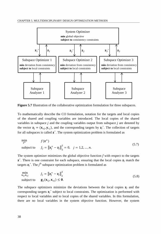
CHAPTER 5. MULTIDISCIPLINARY DESIGN OPTIMIZATION METHODS
Figure 5.7 Illustration of the collaborative optimization formulation for three subspaces.
To mathematically describe the CO formulation, notation for the targets and local copies of the shared and coupling variables are introduced. The local copies of the shared variables in subspace j and the coupling variables output from subspace j are denoted by the vector 𝐳𝑗 = (𝐱𝑠𝑗, 𝐲∗𝑗), and the corresponding targets by zj
+. The collection of targets for all subspaces is called z+. The system optimization problem is formulated as
minz+
𝑓(𝐳+) (5.7)
subject to 𝐽𝑗 = �𝐳𝑗+ − 𝐳𝑗�22
= 0, 𝑗 = 1,2, … ,𝑛.
The system optimizer minimizes the global objective function f with respect to the targets z+. There is one constraint for each subspace, ensuring that the local copies zj match the targets zj
+. The jth subspace optimization problem is formulated as
min𝐱𝑙𝑗,𝐱𝑠𝑗
𝐽𝑗 = �𝐳𝑗+ − 𝐳𝑗�22
(5.8) subject to 𝐠𝑗(𝐱𝑙𝑗, 𝐱𝑠𝑗) ≤ 𝟎.
The subspace optimizers minimize the deviations between the local copies zj and the corresponding targets zj
+ subject to local constraints. The optimization is performed with respect to local variables and to local copies of the shared variables. In this formulation, there are no local variables in the system objective function. However, the system
min deviation from consistencysubject to local constraints
Subspace Analyzer 3
System Optimizer
Subspace Analyzer 2
Subspace Optimizer 1 Subspace Optimizer 3Subspace Optimizer 2
Subspace Analyzer 1
min global objectivesubject to consistency constraints
min deviation from consistencysubject to local constraints
min deviation from consistencysubject to local constraints
z1+ z2
+ z3+z1 z2 z3
38
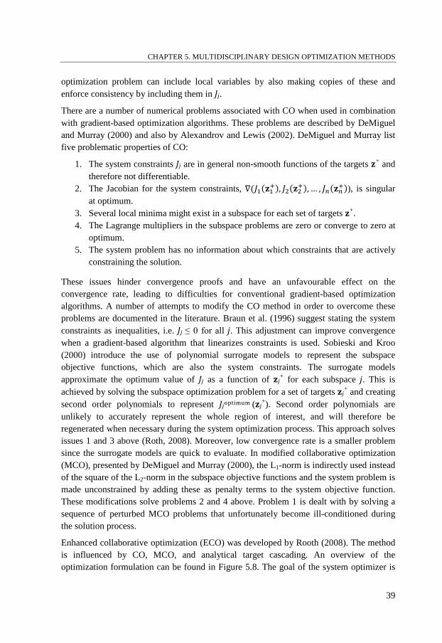
CHAPTER 5. MULTIDISCIPLINARY DESIGN OPTIMIZATION METHODS optimization problem can include local variables by also making copies of these and enforce consistency by including them in Jj.
There are a number of numerical problems associated with CO when used in combination with gradient-based optimization algorithms. These problems are described by DeMiguel and Murray (2000) and also by Alexandrov and Lewis (2002). DeMiguel and Murray list five problematic properties of CO:
1. The system constraints Jj are in general non-smooth functions of the targets z+ and therefore not differentiable.
2. The Jacobian for the system constraints, ∇(𝐽1(𝐳1+), 𝐽2(𝐳2+), … , 𝐽𝑛(𝐳𝑛+)), is singular at optimum.
3. Several local minima might exist in a subspace for each set of targets z+. 4. The Lagrange multipliers in the subspace problems are zero or converge to zero at
optimum. 5. The system problem has no information about which constraints that are actively
constraining the solution.
These issues hinder convergence proofs and have an unfavourable effect on the convergence rate, leading to difficulties for conventional gradient-based optimization algorithms. A number of attempts to modify the CO method in order to overcome these problems are documented in the literature. Braun et al. (1996) suggest stating the system constraints as inequalities, i.e. Jj ≤ 0 for all j. This adjustment can improve convergence when a gradient-based algorithm that linearizes constraints is used. Sobieski and Kroo (2000) introduce the use of polynomial surrogate models to represent the subspace objective functions, which are also the system constraints. The surrogate models approximate the optimum value of Jj as a function of zj
+ for each subspace j. This is achieved by solving the subspace optimization problem for a set of targets zj
+ and creating second order polynomials to represent Jjoptimum (zj
+). Second order polynomials are unlikely to accurately represent the whole region of interest, and will therefore be regenerated when necessary during the system optimization process. This approach solves issues 1 and 3 above (Roth, 2008). Moreover, low convergence rate is a smaller problem since the surrogate models are quick to evaluate. In modified collaborative optimization (MCO), presented by DeMiguel and Murray (2000), the L1-norm is indirectly used instead of the square of the L2-norm in the subspace objective functions and the system problem is made unconstrained by adding these as penalty terms to the system objective function. These modifications solve problems 2 and 4 above. Problem 1 is dealt with by solving a sequence of perturbed MCO problems that unfortunately become ill-conditioned during the solution process.
Enhanced collaborative optimization (ECO) was developed by Rooth (2008). The method is influenced by CO, MCO, and analytical target cascading. An overview of the optimization formulation can be found in Figure 5.8. The goal of the system optimizer is
39
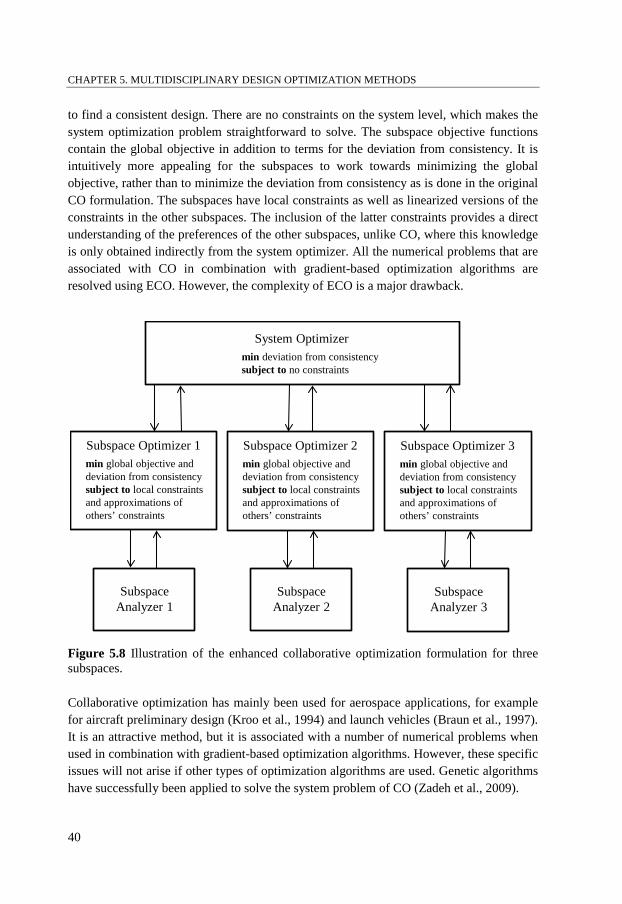
CHAPTER 5. MULTIDISCIPLINARY DESIGN OPTIMIZATION METHODS to find a consistent design. There are no constraints on the system level, which makes the system optimization problem straightforward to solve. The subspace objective functions contain the global objective in addition to terms for the deviation from consistency. It is intuitively more appealing for the subspaces to work towards minimizing the global objective, rather than to minimize the deviation from consistency as is done in the original CO formulation. The subspaces have local constraints as well as linearized versions of the constraints in the other subspaces. The inclusion of the latter constraints provides a direct understanding of the preferences of the other subspaces, unlike CO, where this knowledge is only obtained indirectly from the system optimizer. All the numerical problems that are associated with CO in combination with gradient-based optimization algorithms are resolved using ECO. However, the complexity of ECO is a major drawback.
Figure 5.8 Illustration of the enhanced collaborative optimization formulation for three subspaces.
Collaborative optimization has mainly been used for aerospace applications, for example for aircraft preliminary design (Kroo et al., 1994) and launch vehicles (Braun et al., 1997). It is an attractive method, but it is associated with a number of numerical problems when used in combination with gradient-based optimization algorithms. However, these specific issues will not arise if other types of optimization algorithms are used. Genetic algorithms have successfully been applied to solve the system problem of CO (Zadeh et al., 2009).
System Optimizer
Subspace Optimizer 1
Subspace Analyzer 1
min deviation from consistencysubject to no constraints
min global objective and deviation from consistencysubject to local constraintsand approximations ofothers’ constraints
Subspace Optimizer 2
Subspace Analyzer 2
min global objective and deviation from consistencysubject to local constraintsand approximations ofothers’ constraints
Subspace Optimizer 3
Subspace Analyzer 3
min global objective and deviation from consistencysubject to local constraintsand approximations ofothers’ constraints
40
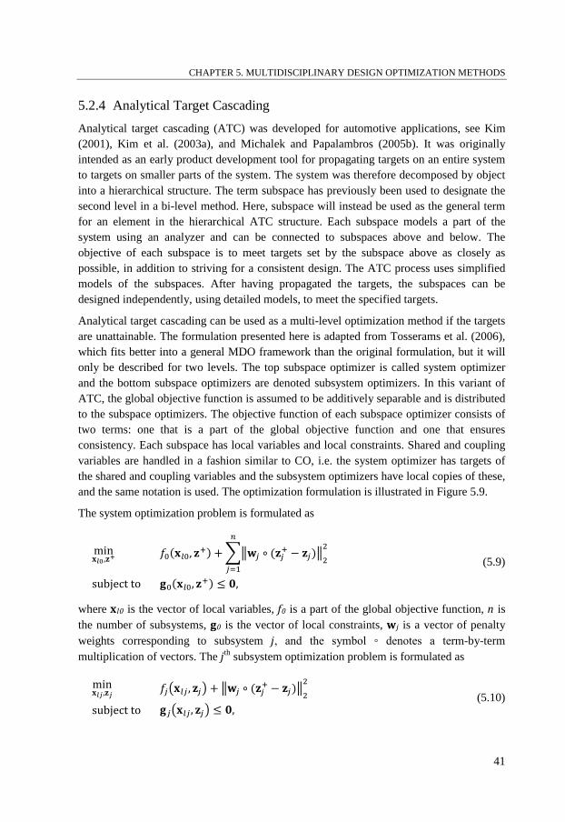
CHAPTER 5. MULTIDISCIPLINARY DESIGN OPTIMIZATION METHODS
5.2.4 Analytical Target Cascading Analytical target cascading (ATC) was developed for automotive applications, see Kim (2001), Kim et al. (2003a), and Michalek and Papalambros (2005b). It was originally intended as an early product development tool for propagating targets on an entire system to targets on smaller parts of the system. The system was therefore decomposed by object into a hierarchical structure. The term subspace has previously been used to designate the second level in a bi-level method. Here, subspace will instead be used as the general term for an element in the hierarchical ATC structure. Each subspace models a part of the system using an analyzer and can be connected to subspaces above and below. The objective of each subspace is to meet targets set by the subspace above as closely as possible, in addition to striving for a consistent design. The ATC process uses simplified models of the subspaces. After having propagated the targets, the subspaces can be designed independently, using detailed models, to meet the specified targets.
Analytical target cascading can be used as a multi-level optimization method if the targets are unattainable. The formulation presented here is adapted from Tosserams et al. (2006), which fits better into a general MDO framework than the original formulation, but it will only be described for two levels. The top subspace optimizer is called system optimizer and the bottom subspace optimizers are denoted subsystem optimizers. In this variant of ATC, the global objective function is assumed to be additively separable and is distributed to the subspace optimizers. The objective function of each subspace optimizer consists of two terms: one that is a part of the global objective function and one that ensures consistency. Each subspace has local variables and local constraints. Shared and coupling variables are handled in a fashion similar to CO, i.e. the system optimizer has targets of the shared and coupling variables and the subsystem optimizers have local copies of these, and the same notation is used. The optimization formulation is illustrated in Figure 5.9.
The system optimization problem is formulated as
min𝐱𝑙0 ,𝐳+
𝑓0(𝐱𝑙0, 𝐳+) + ��𝐰𝑗 ∘ (𝐳𝑗+ − 𝐳𝑗)�2
2𝑛
𝑗=1
(5.9)
subject to 𝐠0(𝐱𝑙0, 𝐳+) ≤ 𝟎,
where xl0 is the vector of local variables, f0 is a part of the global objective function, n is the number of subsystems, g0 is the vector of local constraints, wj is a vector of penalty weights corresponding to subsystem j, and the symbol ◦ denotes a term-by-term multiplication of vectors. The jth subsystem optimization problem is formulated as
min𝐱𝑙𝑗,𝐳𝑗
𝑓𝑗�𝐱𝑙𝑗 , 𝐳𝑗� + �𝐰𝑗 ∘ (𝐳𝑗+ − 𝐳𝑗)�2
2
(5.10) subject to 𝐠𝑗�𝐱𝑙𝑗, 𝐳𝑗� ≤ 𝟎,
41
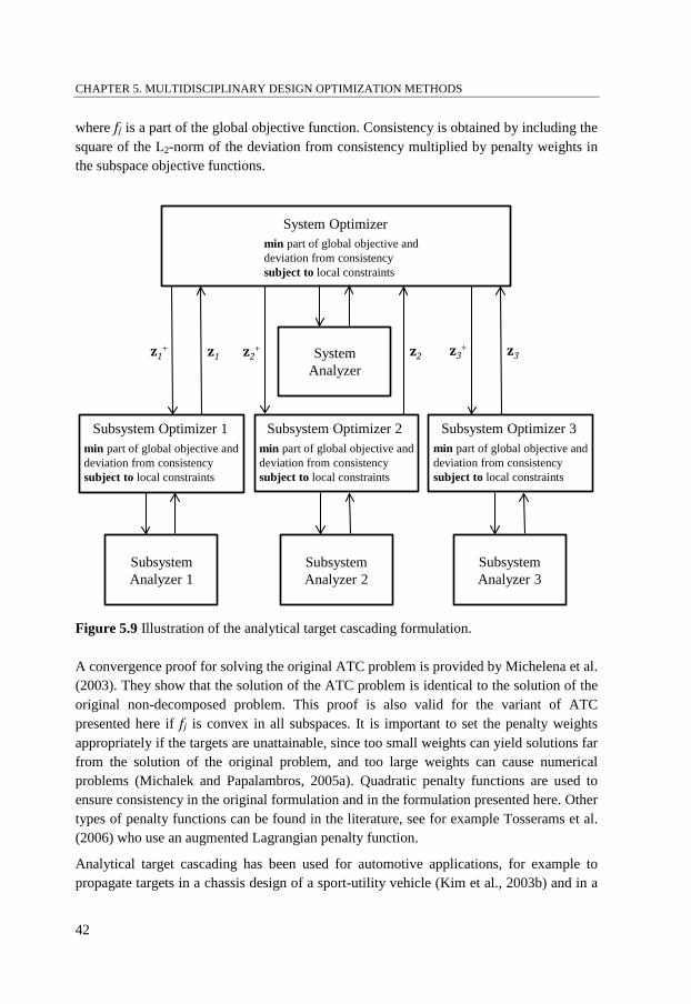
CHAPTER 5. MULTIDISCIPLINARY DESIGN OPTIMIZATION METHODS where fj is a part of the global objective function. Consistency is obtained by including the square of the L2-norm of the deviation from consistency multiplied by penalty weights in the subspace objective functions.
Figure 5.9 Illustration of the analytical target cascading formulation.
A convergence proof for solving the original ATC problem is provided by Michelena et al. (2003). They show that the solution of the ATC problem is identical to the solution of the original non-decomposed problem. This proof is also valid for the variant of ATC presented here if fj is convex in all subspaces. It is important to set the penalty weights appropriately if the targets are unattainable, since too small weights can yield solutions far from the solution of the original problem, and too large weights can cause numerical problems (Michalek and Papalambros, 2005a). Quadratic penalty functions are used to ensure consistency in the original formulation and in the formulation presented here. Other types of penalty functions can be found in the literature, see for example Tosserams et al. (2006) who use an augmented Lagrangian penalty function.
Analytical target cascading has been used for automotive applications, for example to propagate targets in a chassis design of a sport-utility vehicle (Kim et al., 2003b) and in a
Subsystem Analyzer 3
System Optimizer
Subsystem Analyzer 2
Subsystem Optimizer 1 Subsystem Optimizer 3Subsystem Optimizer 2
Subsystem Analyzer 1
min part of global objective and deviation from consistencysubject to local constraints
min part of global objective and deviation from consistencysubject to local constraints
min part of global objective and deviation from consistencysubject to local constraints
min part of global objective and deviation from consistencysubject to local constraints
z1+ z2
+ z3+z1 z2 z3System
Analyzer
42

CHAPTER 5. MULTIDISCIPLINARY DESIGN OPTIMIZATION METHODS redesign of a U.S. class VI truck (Kim et al., 2002). However, none of these studies utilizes ATC as an MDO tool to optimize structures. The method has also been used for aerospace applications. Tosserams et al. (2010) use ATC to minimize the weight of a supersonic business jet.
43

CHAPTER 5. MULTIDISCIPLINARY DESIGN OPTIMIZATION METHODS
44
Metamodel-Based MDO of Automotive Structures
6
The aim of this thesis is to find suitable MDO methods for automotive structural applications. The basics of MDO are covered in Chapter 3, and the characteristics of automotive structural MDO problems are specifically considered. It is concluded that MBDO can be an efficient way to handle the computationally expensive simulation models that need to be evaluated when performing MDO of automotive structures. The principles of MBDO are therefore discussed in Chapter 4. A number of commonly used MDO methods are thereafter investigated in Chapter 5.
In this chapter, a number of requirements that must be fulfilled in order for an MDO method to be suitable for automotive structural applications are stated. Thereafter, the MDO methods covered in Chapter 5 are assessed in relation to these requirements. Finally, a metamodel-based MDO process is suggested.
6.1 Requirements on MDO Methods
The nature of automotive structural MDO problems is considered in Section 3.2. Based on this discussion, a number of requirements imposed on an MDO method for automotive structural applications are now given.
First of all, performing large-scale MDO of automotive structures involves several groups. In order to solve the problem efficiently, the MDO method must allow individual groups to work on the problem concurrently and autonomously. Concurrency means that human and computational resources can be used in parallel, and autonomy that groups can make design decisions and govern methods and tools. Another issue, also related to efficiency, is the handling of the computationally expensive simulation models that are frequently included in automotive MDO studies. In order to reduce the required computational effort, the MDO method must be able to integrate the use of metamodels. Further, coupling variables are seldom present in MDO of automotive structures. This fact simplifies the solution process considerably and should be taken advantage of. The requirements imposed on an MDO method for large-scale automotive structural applications can therefore be summarized as follows:
45
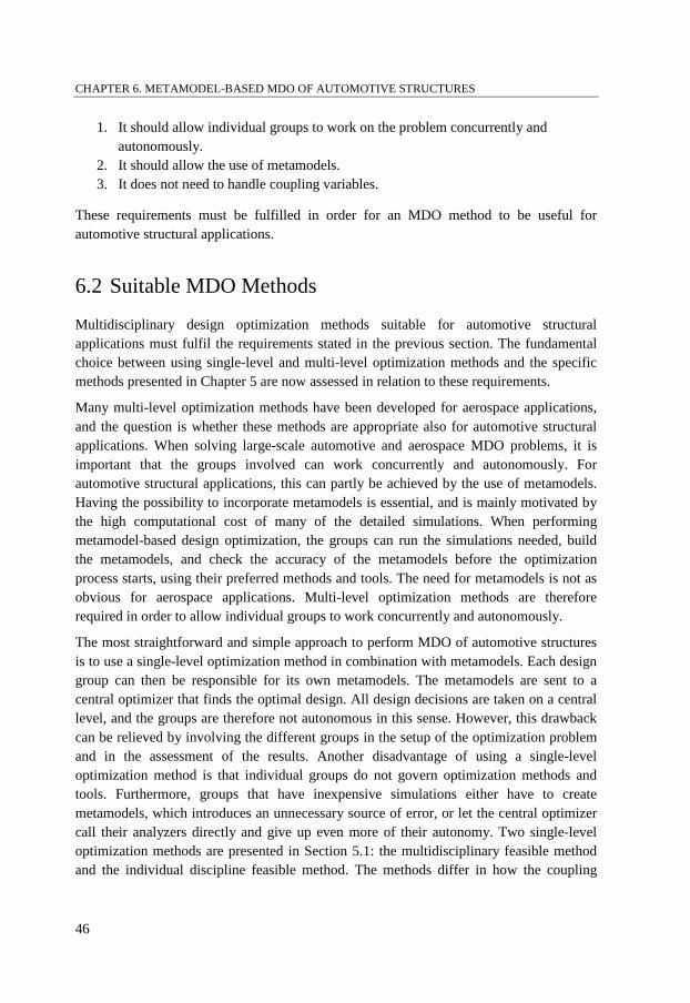
CHAPTER 6. METAMODEL-BASED MDO OF AUTOMOTIVE STRUCTURES
1. It should allow individual groups to work on the problem concurrently and autonomously.
2. It should allow the use of metamodels. 3. It does not need to handle coupling variables.
These requirements must be fulfilled in order for an MDO method to be useful for automotive structural applications.
6.2 Suitable MDO Methods
Multidisciplinary design optimization methods suitable for automotive structural applications must fulfil the requirements stated in the previous section. The fundamental choice between using single-level and multi-level optimization methods and the specific methods presented in Chapter 5 are now assessed in relation to these requirements.
Many multi-level optimization methods have been developed for aerospace applications, and the question is whether these methods are appropriate also for automotive structural applications. When solving large-scale automotive and aerospace MDO problems, it is important that the groups involved can work concurrently and autonomously. For automotive structural applications, this can partly be achieved by the use of metamodels. Having the possibility to incorporate metamodels is essential, and is mainly motivated by the high computational cost of many of the detailed simulations. When performing metamodel-based design optimization, the groups can run the simulations needed, build the metamodels, and check the accuracy of the metamodels before the optimization process starts, using their preferred methods and tools. The need for metamodels is not as obvious for aerospace applications. Multi-level optimization methods are therefore required in order to allow individual groups to work concurrently and autonomously.
The most straightforward and simple approach to perform MDO of automotive structures is to use a single-level optimization method in combination with metamodels. Each design group can then be responsible for its own metamodels. The metamodels are sent to a central optimizer that finds the optimal design. All design decisions are taken on a central level, and the groups are therefore not autonomous in this sense. However, this drawback can be relieved by involving the different groups in the setup of the optimization problem and in the assessment of the results. Another disadvantage of using a single-level optimization method is that individual groups do not govern optimization methods and tools. Furthermore, groups that have inexpensive simulations either have to create metamodels, which introduces an unnecessary source of error, or let the central optimizer call their analyzers directly and give up even more of their autonomy. Two single-level optimization methods are presented in Section 5.1: the multidisciplinary feasible method and the individual discipline feasible method. The methods differ in how the coupling
46
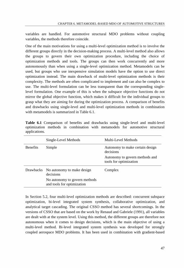
CHAPTER 6. METAMODEL-BASED MDO OF AUTOMOTIVE STRUCTURES variables are handled. For automotive structural MDO problems without coupling variables, the methods therefore coincide.
One of the main motivations for using a multi-level optimization method is to involve the different groups directly in the decision-making process. A multi-level method also allows the groups to govern their own optimization procedure, including the choice of optimization methods and tools. The groups can then work concurrently and more autonomously than when using a single-level optimization method. Metamodels can be used, but groups who use inexpensive simulation models have the option to use direct optimization instead. The main drawback of multi-level optimization methods is their complexity. The methods are often complicated to implement and can also be complex to use. The multi-level formulation can be less transparent than the corresponding single-level formulation. One example of this is when the subspace objective functions do not mirror the global objective function, which makes it difficult for the individual groups to grasp what they are aiming for during the optimization process. A comparison of benefits and drawbacks using single-level and multi-level optimization methods in combination with metamodels is summarized in Table 6.1.
Table 6.1 Comparison of benefits and drawbacks using single-level and multi-level optimization methods in combination with metamodels for automotive structural applications.
Single-Level Methods Multi-Level Methods
Benefits Simple Autonomy to make certain design decisions
Autonomy to govern methods and tools for optimization
Drawbacks No autonomy to make design decisions
Complex
No autonomy to govern methods and tools for optimization
In Section 5.2, four multi-level optimization methods are described: concurrent subspace optimization, bi-level integrated system synthesis, collaborative optimization, and analytical target cascading. The original CSSO method has several shortcomings. In the versions of CSSO that are based on the work by Renaud and Gabriele (1991), all variables are dealt with at the system level. Using this method, the different groups are therefore not autonomous when it comes to design decisions, which is the main objective of using a multi-level method. Bi-level integrated system synthesis was developed for strongly coupled aerospace MDO problems. It has been used in combination with gradient-based
47
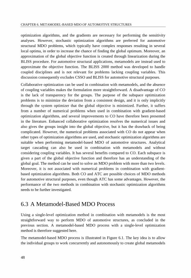
CHAPTER 6. METAMODEL-BASED MDO OF AUTOMOTIVE STRUCTURES optimization algorithms, and the gradients are necessary for performing the sensitivity analyses. However, stochastic optimization algorithms are preferred for automotive structural MDO problems, which typically have complex responses resulting in several local optima, in order to increase the chance of finding the global optimum. Moreover, an approximation of the global objective function is created through linearization during the BLISS procedure. For automotive structural applications, metamodels are instead used to approximate the objective function. The BLISS 2000 method was developed to handle coupled disciplines and is not relevant for problems lacking coupling variables. This discussion consequently excludes CSSO and BLISS for automotive structural purposes.
Collaborative optimization can be used in combination with metamodels, and the absence of coupling variables makes the formulation more straightforward. A disadvantage of CO is the lack of transparency for the groups. The purpose of the subspace optimization problems is to minimize the deviation from a consistent design, and it is only implicitly through the system optimizer that the global objective is minimized. Further, it suffers from a number of numerical problems when used in combination with gradient-based optimization algorithms, and several improvements to CO have therefore been presented in the literature. Enhanced collaborative optimization resolves the numerical issues and also gives the groups insight into the global objective, but it has the drawback of being complicated. However, the numerical problems associated with CO do not appear when other types of optimization algorithms are used, and stochastic optimization algorithms are suitable when performing metamodel-based MDO of automotive structures. Analytical target cascading can also be used in combination with metamodels and without considering coupling variables. It has several benefits compared to CO. Each subspace is given a part of the global objective function and therefore has an understanding of the global goal. The method can be used to solve an MDO problem with more than two levels. Moreover, it is not associated with numerical problems in combination with gradient-based optimization algorithms. Both CO and ATC are possible choices of MDO methods for automotive structural purposes, even though ATC has some advantages. However, the performance of the two methods in combination with stochastic optimization algorithms needs to be further investigated.
6.3 A Metamodel-Based MDO Process
Using a single-level optimization method in combination with metamodels is the most straightforward way to perform MDO of automotive structures, as concluded in the previous section. A metamodel-based MDO process with a single-level optimization method is therefore suggested here.
The metamodel-based MDO process is illustrated in Figure 6.1. The key idea is to allow the individual groups to work concurrently and autonomously to create global metamodels
48
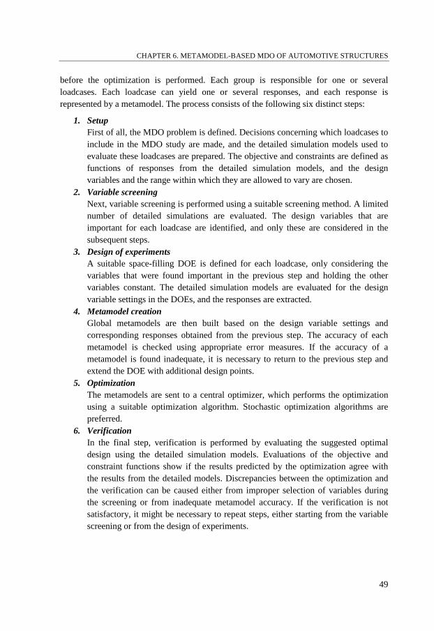
CHAPTER 6. METAMODEL-BASED MDO OF AUTOMOTIVE STRUCTURES before the optimization is performed. Each group is responsible for one or several loadcases. Each loadcase can yield one or several responses, and each response is represented by a metamodel. The process consists of the following six distinct steps:
1. Setup First of all, the MDO problem is defined. Decisions concerning which loadcases to include in the MDO study are made, and the detailed simulation models used to evaluate these loadcases are prepared. The objective and constraints are defined as functions of responses from the detailed simulation models, and the design variables and the range within which they are allowed to vary are chosen.
2. Variable screening Next, variable screening is performed using a suitable screening method. A limited number of detailed simulations are evaluated. The design variables that are important for each loadcase are identified, and only these are considered in the subsequent steps.
3. Design of experiments A suitable space-filling DOE is defined for each loadcase, only considering the variables that were found important in the previous step and holding the other variables constant. The detailed simulation models are evaluated for the design variable settings in the DOEs, and the responses are extracted.
4. Metamodel creation Global metamodels are then built based on the design variable settings and corresponding responses obtained from the previous step. The accuracy of each metamodel is checked using appropriate error measures. If the accuracy of a metamodel is found inadequate, it is necessary to return to the previous step and extend the DOE with additional design points.
5. Optimization The metamodels are sent to a central optimizer, which performs the optimization using a suitable optimization algorithm. Stochastic optimization algorithms are preferred.
6. Verification In the final step, verification is performed by evaluating the suggested optimal design using the detailed simulation models. Evaluations of the objective and constraint functions show if the results predicted by the optimization agree with the results from the detailed models. Discrepancies between the optimization and the verification can be caused either from improper selection of variables during the screening or from inadequate metamodel accuracy. If the verification is not satisfactory, it might be necessary to repeat steps, either starting from the variable screening or from the design of experiments.
49
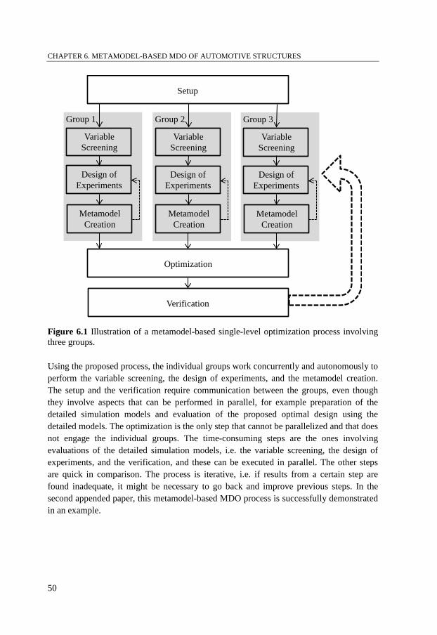
CHAPTER 6. METAMODEL-BASED MDO OF AUTOMOTIVE STRUCTURES
Figure 6.1 Illustration of a metamodel-based single-level optimization process involving three groups.
Using the proposed process, the individual groups work concurrently and autonomously to perform the variable screening, the design of experiments, and the metamodel creation. The setup and the verification require communication between the groups, even though they involve aspects that can be performed in parallel, for example preparation of the detailed simulation models and evaluation of the proposed optimal design using the detailed models. The optimization is the only step that cannot be parallelized and that does not engage the individual groups. The time-consuming steps are the ones involving evaluations of the detailed simulation models, i.e. the variable screening, the design of experiments, and the verification, and these can be executed in parallel. The other steps are quick in comparison. The process is iterative, i.e. if results from a certain step are found inadequate, it might be necessary to go back and improve previous steps. In the second appended paper, this metamodel-based MDO process is successfully demonstrated in an example.
VariableScreening
Setup
Optimization
Verification
Group 1
Design ofExperiments
MetamodelCreation
VariableScreening
Group 2
Design ofExperiments
MetamodelCreation
VariableScreening
Group 3
Design ofExperiments
MetamodelCreation
50
Conclusions 7
The aim of this thesis was to find suitable methods for large-scale MDO of automotive structures. Large-scale MDO problems generally involve several groups who must work concurrently and autonomously for the solution process to be efficient. Further, it must be possible to incorporate metamodels into the MDO process due to the computationally expensive simulation models used in the development of automotive structures.
Single-level optimization methods have a central optimizer that makes all design decisions, while multi-level optimization methods distribute the decision-making process and the control over optimization methods and tools. Multi-level methods are more complex than single-level methods, and if they are to be justified, the benefits of using them must compensate for their complexity.
Single-level optimization methods become more attractive in combination with meta-models, as individual groups can work concurrently and autonomously to create the meta-models before the optimization process starts. This approach requires global metamodels that describe the complete design space. The issue of not participating in design decisions can partly be compensated by involving the groups in the setup of the optimization problem and in the assessment of the results. A single-level optimization method in combination with metamodels is therefore often the most convenient way of solving non-coupled automotive structural MDO problems involving computationally expensive simulation models. This approach is demonstrated by the suggested metamodel-based MDO process, where the individual groups work in parallel to create the metamodels, which are then used by a central optimizer to find the optimal design.
If the benefits of multi-level optimization methods are considered to compensate for the drawbacks, collaborative optimization and analytical target cascading are possible choices. However, analytical target cascading has a number of advantages over collaborative optimization.
51

CHAPTER 7. CONCLUSIONS
52
Review of Appended Papers 8
Paper I
Multidisciplinary design optimization methods for automotive structures In the first paper, MDO methods are assessed in relation to the characteristics of automotive structural applications. Both multi-level optimization formulations, such as collaborative optimization and analytical target cascading, and single-level optimization formulations are investigated. When performing large-scale MDO of automotive structures, several groups must work concurrently and autonomously, metamodels are required, but coupling variables do not have to be considered. A single-level method in combination with metamodels is found to be the most straightforward way of implementing MDO into the development of automotive structures.
Paper II
A metamodel-based multidisciplinary design optimization process for automotive structures The second paper presents a metamodel-based MDO process intended for large-scale automotive structural applications with computationally expensive simulation models. The process is developed to fit into existing organizations and product development processes where different groups work in parallel. Based on the conclusions drawn from the first paper, a single-level optimization method is used. The process is demonstrated in a simple example. It is concluded to be efficient, flexible, and suitable for automotive structural applications. Moreover, improved designs can be found even when using metamodels with limited accuracy.
53

CHAPTER 8. REVIEW OF APPENDED PAPERS
54
Bibliography
Agte, J., de Weck, O., Sobieszczanski-Sobieski, J., Arendsen, P., Morris, A., and Spieck,
M. (2010). MDO: Assessment and direction for advancement - An opinion of one international group. Structural and Multidisciplinary Optimization, 40(1-6), 17-33.
Alexandrov, N. (2005). Editorial - Multidisciplinary design optimization. Optimization and Engineering, 6(1), 5-7.
Alexandrov, N. M., and Lewis, R. M. (2002). Analytical and computational aspects of collaborative optimization for multidisciplinary design. AIAA Journal, 40(2), 301-309.
Allison, J., Kokkolaras, M., and Papalambros, P. (2005). On the impact of coupling strength on complex system optimization for single-level formulations. DETC2005-84790. ASME International Design Engineering Technical Conferences & Computers and Information in Engineering Conference. Long Beach, California, September 24-28.
Balling, R. J., and Sobieszczanski-Sobieski, J. (1994). Optimization of coupled systems: A critical overview of approaches. AIAA-94-4330-CP. 5th AIAA/USAF/NASA/ ISSMO Symposium on Multidisciplinary Analysis and Optimization. Panama City Beach, Florida, September 7-9.
Bendsøe, M. P., and Sigmund, O. (2003). Topology optimization: Theory, methods and applications (2nd ed.). Berlin: Springer.
Bishop, C. M. (1995). Neural networks for pattern recognition. Oxford: Oxford University Press.
Bloebaum, C. L., Hajela, P., and Sobieszczanski-Sobieski, J. (1992). Non-hierarchic system decomposition in structural optimization. Engineering Optimization, 19, 171-186.
Braun, R. D. (1996). Collaborative optimization: An architecture for large-scale distri-buted design. Ph.D. thesis, Department of Aeronautics and Astronautics, Stanford University.
55
BIBLIOGRAPHY Braun, R., Gage, P., Kroo, I., and Sobieski, I. (1996). Implementation and performance
issues in collaborative optimization. AIAA-96-4017-CP. 6th NASA/ISSMO Symposium on Multidisciplinary Analysis and Optimization. Bellevue, Washington, September 4-6.
Braun, R. D., Moore, A. A., and Kroo, I. M. (1997). Collaborative approach to launch vehicle design. Journal of Spacecraft and Rockets, 34(4), 478-486.
Craig, K. J., Stander, N., Dooge, D. A., and Varadappa, S. (2002). MDO of automotive vehicle for crashworthiness and NVH using response surface methods. AIAA 2002-5607. 9th AIAA/ISSMO Symposium on Multidisciplinary Analysis and Optimization. Atlanta, Georgia, September 4-6.
Cramer, E. J., Dennis Jr., J. E., Frank, P. D., Lewis, R. M., and Shubin, G. R. (1994). Problem formulation for multidisciplinary optimization. SIAM Journal on Optimization, 4(4), 754-776.
DeMiguel, A. V., and Murray, W. (2000). An analysis of collaborative optimization methods. AIAA-2000-4720. 8th AIAA/USAF/NASA/ISSMO Symposium on Multidisciplinary Analysis and Optimization. Long Beach, California, September 6-8.
Duddeck, F. (2008). Multidisciplinary optimization of car bodies. Structural and Multidisciplinary Optimization, 35(4), 375-389.
Eiben, A. E., and Smith, J. E. (2003). Introduction to evolutionary computing. Berlin: Springer.
Gallagher, R. H. (1973). Terminology and basic concepts. In R. H. Gallagher, and O. C. Zienkiewicz (Eds.), Optimum structural design: Theory and applications (pp. 7-17). London: Wiley.
Giesing, J. P., and Barthelemy, J.-F. M. (1998). A summary of industry MDO applications and needs. 7th AIAA/USAF/NASA/ISSMO Symposium on Multidisciplinary Analysis and Optimization. St. Louis, Missouri, September 2-4.
Haftka, R. T., Sobieszczanski-Sobieski, J., and Padula, S. L. (1992). On options for interdisciplinary analysis and design optimization. Structural Optimization, 4(2), 65-74.
Johnson, M., Moore, L., and Ylvisaker, D. (1990). Minimax and maximin distance designs. Journal of Statistical Planning and Inference, 26(2), 131-148.
Kim, H. M. (2001). Target cascading in optimal system design. Ph.D. thesis, Mechanical Engineering, University of Michigan, Ann Arbor.
56
BIBLIOGRAPHY
Kim, H. M., Kokkolaras, M., Louca, L. S., Delagrammatikas, G. J., Michelena, N. F., Filipi, Z. S., Papalambros, P. Y., Stein, J. L., and Assanis, D. N. (2002). Target cascading in vehicle redesign: A class VI truck study. International Journal of Vehicle Design, 29(3), 199-225.
Kim, H. M., Michelena, N. F., Papalambros, P. Y., and Jiang, T. (2003a). Target cascading in optimal system design. Journal of Mechanical Design, Transactions Of the ASME, 125(3), 474-480.
Kim, H., Ragon, S., Soremekun, G., Malone, B., and Sobieszczanski-Sobieski, J. (2004). Flexible approximation model approach for bi-level integrated system synthesis. AIAA 2004-4545. 10th AIAA/ISSMO Multidisciplinary Analysis and Optimization Conference. Albany, New York, August 30 - September 1.
Kim, H. M., Rideout, D. G., Papalambros, P. Y., and Stein, J. L. (2003b). Analytical target cascading in automotive vehicle design. Journal of Mechanical Design, Transactions of the ASME, 125(3), 481-489.
Kodiyalam, S., and Sobieszczanski-Sobieski, J. (2000). Bilevel integrated system synthesis with response surfaces. AIAA journal, 38(8), 1479-1485.
Kodiyalam, S., and Sobieszczanski-Sobieski, J. (2001). Multidisciplinary design optimi-zation - Some formal methods, framework requirements, and application to vehicle design. International Journal of Vehicle Design, 25(1-2 SPEC. ISS.), 3-22.
Kodiyalam, S., Yang, R. J., Gu, L., and Tho, C.-H. (2004). Multidisciplinary design optimization of a vehicle system in a scalable, high performance computing environment. Structural and Multidisciplinary Optimization, 26(3), 256-263.
Kroo, I., Altus, S., Braun, R., Gage, P., and Sobieski, I. (1994). Multidisciplinary optimization methods for aircraft preliminary design. AIAA-94-4325-CP. 5th AIAA/USAF/NASA/ISSMO Symposium on Multidisciplinary Analysis and Optimization. Panama City Beach, Florida, September 7-9.
Kroo, I., and Manning, V. (2000). Collaborative optimization: Status and directions. AIAA-2000-4721. 8th AIAA/USAF/NASA/ISSMO Symposium on Multidisciplinary Analysis and Optimization. Long Beach, California, September 6-8.
McKay, M. D., Beckman, R. J., and Conover, W. J. (1979). A comparison of three methods for selecting values of input variables in the analysis of output from a computer code. Technometrics, 21(2), 239-245.
Michalek, J. J., and Papalambros, P. Y. (2005a). An efficient weighting update method to achieve acceptable consistency deviation in analytical target cascading. Journal of Mechanical Design, Transactions of the ASME, 127(2), 206-214.
57
BIBLIOGRAPHY Michalek, J. J., and Papalambros, P. Y. (2005b). Weights, norms, and notation in
analytical target cascading. Journal of Mechanical Design, Transactions of the ASME, 127(3), 499-501.
Michelena, N., Park, H., and Papalambros, P. Y. (2003). Convergence properties of analytical target cascading. AIAA Journal, 41(5), 897-905.
Myers, R. H., Montgomery, D. C., and Andersson-Cook, C. M. (2008). Response surface methodology: Process and product optimization using designed experiments (3rd ed.). Hoboken, New Jersey: Wiley.
Pan, J., and Diaz, A. R. (1989). Some results in optimization of non-hierarchic systems. The 1989 ASME Design Technical Conferences - 15th Design Automation Conference. Montreal, Quebec, September 17-21.
Renaud, J. E., and Gabriele, G. A. (1991). Sequential global approximation in non-hierarchic system decomposition and optimization. 17th Design Automation Conference presented at the 1991 ASME Design Technical Conferences. Miami, Florida, September 22-25.
Renaud, J. E., and Gabriele, G. A. (1993). Improved coordination in nonhierarchic system optimization. AIAA journal, 31(12), 2367-2373.
Renaud, J. E., and Gabriele, G. A. (1994). Approximation in nonhierarchic system optimization. AIAA journal, 32(1), 198-205.
Roth, B. D. (2008). Aircraft family design using enhanced collaborative optimization. Ph.D. thesis, Department of Aeronautics and Astronautics, Stanford University.
Ryberg, A.-B., Bäckryd, R. D., and Nilsson, L. (2012). Metamodel-based multidisciplinary design optimization for automotive applications. Technical Report LIU-IEI-R-12/003, Department of Management and Engineering, Linköping University.
Sellar, R. S., Batill, S. M., and Renaud, J. E. (1996). Response surface based, concurrent subspace optimization for multidisciplinary system design. AIAA 96-0714. 34th Aerospace Sciences Meeting and Exhibit. Reno, Nevada, January 15-18.
Shankar, J., Haftka, R. T., and Watson, L. T. (1993). Computational study of a nonhierarchical decomposition algorithm. Computational Optimization and Applications, 2(3), 273-293.
Simpson, T. W., Peplinski, J. D., Koch, P. N., and Allen, J. K. (2001). Metamodels for computer-based engineering design: Survey and recommendations. Engineering with Computers, 17(2), 129-150.
Sobieski, I. P., and Kroo, I. M. (2000). Collaborative optimization using response surface estimation. AIAA journal, 38(10), 1931-1938.
58
BIBLIOGRAPHY
Sobieszczanski-Sobieski, J. (1988). Optimization by decomposition: A step from hierarchic to non-hierarchic systems. Second NASA/Air Force Symposium on Recent Advances in Multidisciplinary Analysis and Optimization. Hampton, Virginia, September.
Sobieszczanski-Sobieski, J. (1990). Sensitivity of complex, internally coupled systems. AIAA journal, 28(1), 153-160.
Sobieszczanski-Sobieski, J., Agte, J. S., and Sandusky Jr., R. R. (1998). Bi-level integrated system synthesis (BLISS). AIAA-98-4916. 7th AIAA/USAF/NASA/ ISSMO Symposium on Multidisciplinary Analysis and Optimization. St. Louis, Missouri, September 2-4.
Sobieszczanski-Sobieski, J., Altus, T. D., Phillips, M., and Sandusky, R. (2003). Bilevel integrated system synthesis for concurrent and distributed processing. AIAA Journal, 41(10), 1996-2003.
Sobieszczanski-Sobieski, J., and Haftka, R. T. (1987). Interdisciplinary and multilevel optimum design. In C. M. Soares (Ed.), Computer aided optimal design: Structural and mechanical systems (pp. 655-701). Berlin: Springer.
Sobieszczanski-Sobieski, J., Kodiyalam, S., and Yang, R. Y. (2001). Optimization of car body under constraints of noise, vibration, and harshness (NVH), and crash. Structural and Multidisciplinary Optimization, 22(4), 295-306.
Sobol', I. M. (2001). Global sensitivity indices for nonlinear mathematical models and their Monte Carlo estimates. Mathematics and Computers in Simulation, 55(1-3), 271-280.
Stander, N., Roux, W., Goel, T., Eggleston, T., and Craig, K. (2012). LS-OPT user's manual version 4.2. Livermore: Livermore Software Technology Corporation.
Tedford, N. P., and Martins, J. R. (2006). On the common structure of MDO problems: A comparison of architectures. AIAA 2006-7080. 11th AIAA/ISSMO Multi-disciplinary Analysis and Optimization Conference. Portsmouth, Virginia, September 6-8.
Tosserams, S., Etman, L. F., Papalambros, P. Y., and Rooda, J. E. (2006). An augmented lagrangian relaxation for analytical target cascading using the alternating direction method of multipliers. Structural and Multidisciplinary Optimization, 31(3), 176-189.
Tosserams, S., Kokkolaras, M., Etman, L. F., and Rooda, J. E. (2010). A nonhierarchical formulation of analytical target cascading. Journal of Mechanical Design, Transactions of the ASME, 132(5), 510021-5100213.
59
BIBLIOGRAPHY Venter, G. (2010). Review of optimization techniques. In R. Blockley, and W. Shyy
(Eds.), Encyclopedia of aerospace engineering (Vol. 8: System Engineering). Chichester, West Sussex: Wiley.
Viana, F. A., Gogu, C., and Haftka, R. T. (2010). Making the most out of surrogate models: Tricks of the trade. DETC2010-28813. Proceedings of the ASME 2010 International Design Engineering Technical Conferences & Computers and Information in Engineering Conference. Montreal, Quebec, August 15-18.
Wang, G. G., and Shan, S. (2007). Review of metamodeling techniques in support of engineering design optimization. Journal of Mechanical Design, 129(4), 370-380.
Wujek, B. A., Renaud, J. E., Batill, S. M., and Brockman, J. B. (1995). Concurrent subspace optimization using design variable sharing in a distributed computing environment. Proceedings of the 1995 ASME Design Engineering Technical Conference. Boston, Massachusetts, September 17-20.
Zadeh, P. M., Toropov, V. V., and Wood, A. S. (2009). Metamodel-based collaborative optimization framework. Structural and Multidisciplinary Optimization, 38(2), 103-115.
60