multifrequencyramangenerationinthe transientregime athesis
TRANSCRIPT

Multifrequency Raman Generation in the Transient Regime
by
Fraser Cunningham Turner
A thesis presented to the University of Waterloo
in fulfilment of the thesis requirement for the degree of
Master of Science in
Physics
Waterloo, Ontario, Canada, 2006
©Fraser Cunningham Turner 2006

ii
Author's Declaration for Electronic Submission of a Thesis I hereby declare that I am the sole author of this thesis. This is a true copy of the thesis, including any required final revisions, as accepted by my examiners. I understand that my thesis may be made electronically available to the public.
iii
Abstract Two colour pumping was used to investigate the short-pulse technique of Multifrequency
Raman Generation (MRG) in the transient regime of Raman scattering. In the course of this
study we have demonstrated the ability to generate over thirty Raman orders spanning from
the infrared to the ultraviolet, investigated the dependence of this generation on the pump
intensities and the dispersion characteristics of the hollow-fibre system in which the
experiment was conducted, and developed a simple computer model to help understand the
exhibited behaviours. These dependence studies have revealed some characteristics that
have been previously mentioned in the literature, such as the competition between MRG and
self-phase modulation, but have also demonstrated behaviours that are dramatically different
than anything reported on the subject. Furthermore, through a simple modification of the
experimental apparatus we have demonstrated the ability to scatter a probe pulse into many
Raman orders, generating bandwidth comparable to the best pump-probe experiments of
MRG. By using a numeric fast Fourier transform, we predict that our spectra can generate
pulses as short as 3.3fs, with energies an order of magnitude larger than pulses of
comparable duration that are made using current techniques.

iv
Acknowledgements First and foremost, I wish to thank my supervisor Dr. Donna Strickland for the fantastic
experience I have had working in her research lab. Under her guidance I had the
opportunity to participate in conferences and collaborations that have served to advance my
professional skills and experience, far beyond what I expected when I first came to
Waterloo. Her patience with my frequent visits (and the occasional argumentativeness),
coupled with her endless encouragement has allowed me to feel free to express my opinions
and explore what I felt to be important, and for this freedom I am very grateful.
I would also like to thank Dr. Joseph Sanderson, whom in essence was my second
supervisor, always willing to discuss my work and lend a wrench or waveplate when needed.
Many parts of this experiment were developed or maintained by his group, such as the
hollow-fibre apparatus, its vacuum system, and the front-end oscillator. Without these
contributions, this experiment would not have been available to me for my Masters.
For being on my defence committee and giving excellent suggestions for this thesis, I wish
to thank Dr. Kostadinka Bizheva, Dr. Joseph Sanderson, and Dr. Donna Strickland. I also
wish to thank Dr. Jim Martin for being on my Masters committee these last two years.
I sincerely thank Dr. Alexandre Trottier for training me in the particulars of using this laser
system, and for his extensive input and development of this experiment. As well, I would
like to thank Dr. Leonid Losev, for his original idea to use this laser system to study MRG,
his assistance in the experiment, and the use of one of his published figures (Figure 2-3).
A wholehearted thank you goes to the community of students and staff at the University of
Waterloo, who have helped with this project through useful discussions, assistance in the
building, maintaining, and conducting the experiment, or for their own work towards the
developing the apparatus. In particular I would like to thank Andy Colclough, Rob Helsten,
Steve Walker, JP Brichta, Jeremy Roth, Owen Cherry, Jeff Carter, and all of the professionals
in the Machine and Electronics shop of the University of Waterloo.
I would also like to thank Newport for the use of one of its illustrations (Figure 4-1).

v
Table of Contents
1. Introduction to Multifrequency Raman Generation..............................................................1 1.1. Historical Context..............................................................................................................1 1.2. General Description of MRG..........................................................................................3 1.3. Historical Development of MRG....................................................................................6
2. Theory.........................................................................................................................................13 2.1. Classical description.........................................................................................................13 2.2. Characteristics of MRG ..................................................................................................21 2.3. Computational model......................................................................................................26
3. Experimental Apparatus ..........................................................................................................30 3.1. Front-End Laser System & Pulse Stretcher .................................................................31 3.2. Dual-Wavelength Regenerative Amplifier....................................................................33 3.3. Multipass Amplifier .........................................................................................................38 3.4. Grating Compressor and Autocorrelator .....................................................................40 3.5. Hollow Fibre Assembly ..................................................................................................43 3.6. Diagnostics........................................................................................................................47
4. Experimental Results & Discussion.......................................................................................51 4.1. Procedure and Measurement..........................................................................................51 4.2. Demonstration of Broadband MRG.............................................................................55 4.3. Demonstration of Pump-Probe MRG .........................................................................56 4.4. Five-pass Amplifier..........................................................................................................58 4.5. Intensity Scan ...................................................................................................................60 4.6. Modelling Transient MRG .............................................................................................63 4.7. Pressure and Dispersion .................................................................................................65
5. Concluding Comments ............................................................................................................72 Appendix A: Modelling the Regenerative Amplifier.................................................................74
A.1 ABCD Matrices................................................................................................................74 A.2 Gaussian Beams ...............................................................................................................77 A.3 Modelling a Laser Cavity.................................................................................................79 A.4 Results of the program....................................................................................................82
Appendix B: Alignment.................................................................................................................86 B.1 Plane Mirrors ....................................................................................................................86 B.2 Lenses ................................................................................................................................88 B.3 Prisms ................................................................................................................................89 B.4 Gratings .............................................................................................................................90 B.5 Grating Compressor ........................................................................................................91 B.6 Pockels Cell.......................................................................................................................91 B.7 Building the Regenerative Amplifier .............................................................................93
Appendix C: Computer Code.......................................................................................................98 References .........................................................................................................................................104

vi
List of Illustrations
Figure 1-1: Illustration of MRG ............................................................................................................................................4 Figure 1-2: Vibrating molecule frequency-modulating an input probe.........................................................................4 Figure 1-3: Energy level diagram of MRG. .........................................................................................................................6 Figure 1-4: Origin of the phase-matching angles ...............................................................................................................6 Figure 1-5: Two configurations for generating sidebands ................................................................................................7 Figure 2-1: Vibrating diatomic molecule ...........................................................................................................................14 Figure 2-2: Plot of the parametric growth rate as a function of the Raman parameter ...........................................26 Figure 2-3: Comparison of the program to published results........................................................................................27 Figure 2-4: Resulting spectrum from on-resonance excitation with zero dispersion. ...............................................28 Figure 2-5: Fast Fourier transform of the spectrum in Figure 2-4a.............................................................................29 Figure 3-1: Block Diagram of the Experimental Apparatus ..........................................................................................30 Figure 3-2: Index of refraction curve for SF6 ...................................................................................................................31 Figure 3-3: Effect of various orders of the dispersion on a short pulse ......................................................................32 Figure 3-4: Measured spectrum of the Femtolasers Scientific Pro oscillator..............................................................33 Figure 3-5: Illustration of the dual-wavelength regenerative amplifier.........................................................................33 Figure 3-6: Two-colour seeding of the Regen ..................................................................................................................34 Figure 3-7: Characteristic trace of the fast diode from behind the curved mirror in the Regen. ............................36 Figure 3-8: Signal from a diode placed directly in the beam ..........................................................................................37 Figure 3-9: Illustration of the divergence of the two pulses as they propagate through the crystal. ......................38 Figure 3-10: Illustration of the multipass amplifier when working in a three-pass operation .................................39 Figure 3-11: Negative dispersion.........................................................................................................................................40 Figure 3-12: Single-shot non-collinear autocorrelator.....................................................................................................41 Figure 3-13: Sum-frequency generation using two identical non-collinear pulses .....................................................42 Figure 3-14: Sample Autocorrelation .................................................................................................................................42 Figure 3-15: Scans using the autocorrelator ......................................................................................................................43 Figure 3-16: Balance between the normal dispersion of SF6 and the negative dispersion of the hollow fibre.....44 Figure 3-17: Illustration of the hollow fibre apparatus ...................................................................................................45 Figure 3-18: Alignment of the hollow fibre ......................................................................................................................47 Figure 3-19: Schematic of the measurement apparatus .................................................................................................48 Figure 3-20: Typical plot from the Oriel Spectrometer ..................................................................................................49 Figure 3-21: Generating a linear regression with the spectrometer. .............................................................................49 Figure 3-22: Compiled spectrum.........................................................................................................................................50 Figure 4-1: Early Ando spectrum and reflectivity curve of a mirror used after the hollow fibre, © Newport Corporation – Used by permission.....................................................................................................................................52 Figure 4-2: Anomalous behaviour of an absorptive filter vs. integration time ...........................................................53 Figure 4-3: Two consecutive spectrometer plots where an extra filter had been added...........................................54 Figure 4-4: Generated MRG spectrum using two compressed pulses with a total energy of 1.8mJ. .....................55 Figure 4-5: Comparison between compilation methods for the spectrometer...........................................................56 Figure 4-6: Modulated probe beam ....................................................................................................................................57 Figure 4-7: Pressure scan of the modulated probe ..........................................................................................................58 Figure 4-8: Two MRG spectra with strong SPM .............................................................................................................59 Figure 4-9: Spectra obtained with a five-pass amplifier ..................................................................................................59 Figure 4-10: Variation of the generated bandwidth with total pulse energy ...............................................................60 Figure 4-11: Fourier transform of a 3THz-broad peak on a 50THz base ...................................................................62 Figure 4-12: Number of anti-Stokes orders relative to the short-wavelength pump beam......................................62 Figure 4-13: Modelling transient MRG with Gaussian pulses .......................................................................................64 Figure 4-14: Comparison between experiment and computer model ..........................................................................65 Figure 4-15: Demonstration of how dispersion affects transient MRG. .....................................................................67 Figure 4-16: Dependence of the spectra with pressure on a linear scale .....................................................................67 Figure 4-17: The dependence of the generated spectrum with pressure on a logarithmic scale .............................68 Figure 4-18: A reproduction of Figure 4-17 overlaid with a plot of the group delay relative to the short-wavelength pump. ..................................................................................................................................................................69 Figure 4-19: Series of spectra taken at three atmospheres..............................................................................................70 Figure 4-20: Mapping of the position of the peaks with pressure ................................................................................71 Figure 5-1: Fast Fourier Transforms ..................................................................................................................................72

1
1. Introduction to Multifrequency Raman Generation
1.1. Historical Context The field of high-intensity laser systems has been of keen interest to researchers since the
original harnessing of stimulated emission [Gordon 1954]. With the development of the
laser [Maiman 1960], the unprecedented intensities available in the optical regime quickly led
to research in non-linear optical processes, such as second harmonic generation [Franken
1961]. As these effects depend on the intensity of the laser as opposed to simply the energy,
the growth of this field depended not only on increasing the output from lasers but also on
the development of techniques that shortened the pulses in time. Within the first few years
of developing the laser, the key short-pulse techniques of Q-switching [McClung 1962] and
mode-locking of lasers in the optical regime [Hargrove 1964] had become established,
quickly reducing the pulse lengths from their original microsecond time-scale [Maiman 1961]
down to a few picoseconds [Armstrong 1967]. Further advances in laser technology allowed
researchers to take advantage of these short timescales to generate solid-state lasers with
peak powers approaching 1TW [Seka 1980] – almost a 9 order of magnitude increase from
the original 5kW laser [Maiman 1961]. At these incredible powers however, the nonlinear
index of refraction – an effect present in all bulk materials – causes a self-focussing of the
wavefront as it passes through the gain medium, resulting in a reduced beam quality and
possible damage to the crystals themselves [Fleck 1973]. This effect put major constraints
on high-power systems, necessitating the use of multiple beams to increase the power
delivered in high-intensity experiments [Speck 1981].
These TW-scale lasers developed in the 1970s often used pulses with durations in the
tens to hundreds of picoseconds range, relying more on increasing the energy in the pulse
than decreasing its length to achieve higher intensities. At the same time as these advances
were being made, the alternative pulse-duration approach to high intensity lasers was steadily
maturing – reaching the 100 femtosecond mark around the same time as the laser fusion
facilities were operational [Fork 1981], and breaking 10fs a few years later through the
combination of self-phase modulation in single-mode fibres, and pulse compression
techniques utilizing negative dispersion [Treacy 1969; Fork 1984; Knox 1985]. At this point
the discovery of the impressive lasing properties of titanium-doped sapphire crystals
(Ti:Sapphire) [Lacovara 1985], and the development of Chirped Pulse Amplification

2
[Strickland 1985], allowed for significant advances over the current state of the art dye lasers
and doped-glass lasers. The ability to avoid self-focussing by stretching the pulses before
amplification quickly resulted in tabletop laser systems reaching close to 1TW [Maine 1988],
while the unprecedented bandwidth available in Ti:Sapphire lasers eventually propelled
short-pulsed laser systems to the petawatt level [Perry 1999].
Out of this ultrafast boon also emerged the study of the time evolution of ultrafast
processes, such as observing the transition-state dynamics of chemical reactions and
molecular motion [Zewail 1991]. Analogous to the shutter speed of a camera, shorter pulses
allowed for faster snapshots of these processes, providing further motivation to generate as
short a pulse as possible. While techniques utilizing self-phase modulation and adaptive
compression would eventually produce pulses with durations of 2.8fs [Yamashita 2006], a
fundamental limit was being reached as these pulses approached a single cycle of their
central frequency. To achieve a pulse with a duration of half an optical period, which in the
case of Yamashita et al (2006) was 1fs, the laser would require a bandwidth equal to twice
that of the central frequency, stretching from 0Hz to 02ω . Any further decrease in the pulse
duration would therefore require a shift to a higher central frequency, however as the
technique of self-broadening in hollow waveguides is a relatively mature technology [Nisoli
1996], any significant improvement in the pulse duration would require new techniques to
generate these large bandwidths at much shorter wavelengths.
The most promising technique in the push to break this 1fs barrier grew out of the
effort to produce coherent short-wavelength radiation for x-ray spectroscopy [Harris 1973].
It was found that when an intense IR laser was focussed into a gas, many harmonic orders of
the pump frequency were generated in a characteristic way: the intensity of the first number
of harmonics dropped rapidly, but eventually levelled off into a plateau until finally reaching
some cut-off intensity [Ferray et al. 1988]. It was soon realized that the bandwidth generated
with this High-Harmonic Generation (HHG), could produce temporal structure on the scale
of tens of attoseconds if properly phased [Farkas 1992]. The resulting pulse could then be
used as a probe for processes on the timescale of a Bohr orbit of an electron! With a deeper
understanding of the dynamics involved [Corkum 1993], it was realized that the generated
vuv/X-ray radiation would need minimal phase control, and that while it might not be
perfectly phased, it should automatically produce a train of pulses with durations of
hundreds of attoseconds [Corkum 1994]: an order of magnitude shorter than those
3
generated using continuum techniques. The ensuing development eventually led to the
isolation and measurement of a single attosecond-scale pulse [Hentschel 2001], and a record
pulse duration of 250as [Kienberger 2004].
While this technique has provided unprecedented access to short timescales, its
major drawback lies in the relatively low energy in the pulses, as the conversion efficiency
into usable radiation is quoted as being anywhere from 10-3 to 10-8 [Kaplan 1996; Shon 2002;
Sali 2005]. This low conversion is also a shortcoming of the latest continuum generation
pulses, where each decrease in the pulse length accompanies a dramatic drop in energy: from
5.3fs with 300µJ [Rauschenberger 2006], to 3.8fs with 25µJ [Steinmeyer 2006], to 2.8fs with
0.5µJ [Yamashita 2006]. However, it is the conversion efficiency in which the technique of
Multifrequency Raman Generation (MRG) excels, providing access to timescales on the
order of a femtosecond while allowing conversion of the pump into usable broadband
radiation with efficiencies approaching 100% [Losev 1993; Nazarkin 1999a]. Having
demonstrated the generation of pulse trains with pulses as short as 1.6fs [Shverdin 2005],
and isolated pulses comparable to the best synthesized using continuum generation
[Zhavoronkov 2002], new developments in MRG are showing the potential to generate few-
femtosecond pulses with an order of magnitude more energy than current state-of-the-art
techniques [Turner 2006].
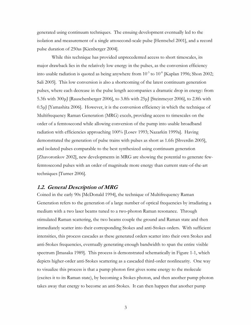
1.2. General Description of MRG Coined in the early 90s [McDonald 1994], the technique of Multifrequency Raman
Generation refers to the generation of a large number of optical frequencies by irradiating a
medium with a two laser beams tuned to a two-photon Raman resonance. Through
stimulated Raman scattering, the two beams couple the ground and Raman state and then
immediately scatter into their corresponding Stokes and anti-Stokes orders. With sufficient
intensities, this process cascades as these generated orders scatter into their own Stokes and
anti-Stokes frequencies, eventually generating enough bandwidth to span the entire visible
spectrum [Imasaka 1989]. This process is demonstrated schematically in Figure 1-1, which
depicts higher-order anti-Stokes scattering as a cascaded third-order nonlinearity. One way
to visualize this process is that a pump photon first gives some energy to the molecule
(excites it to its Raman state), by becoming a Stokes photon, and then another pump photon
takes away that energy to become an anti-Stokes. It can then happen that another pump

4
photon excites the molecule, but instead the anti-Stokes photon generated before absorbs
the energy, producing a second-order anti-Stokes photon.
Figure 1-1: (a) Schematic representation of cascaded anti-Stokes scattering in MRG. Colours from red to violet are taken to be increasing in energy. Assumed in the diagram is that the scattering of the pump beam is stimulated by the introduction of its Stokes radiation at
RamanPumpStokes ωωω −=
(b) Example of a discrete MRG spectrum as dispersed by a prism. The orders shown in light purple are actually in the infrared. This picture was taken in the laboratory of Dr. Strickland.
Alternatively one could consider a classical picture, where the beating two-colour
pump beam excites (for example), vibrations in the molecules of interest. The oscillating
molecules will then act as a frequency modulator, impressing sidebands on the pump beams
in much the same way that acoustic vibrations can be used to phase modulate radio waves in
frequency-modulated (FM) radio. A good experimental demonstration of this FM-like
behaviour is reported in Nazarkin et al (1999), where a probe injected into excited molecules
generated a spectrum strikingly similar to that produced in FM radio (for a good illustration
of an FM spectrum, see http://cnyack.homestead.com/files/modulation/modfm.htm).
This can be thought of as being due to the change in the index of refraction as the molecule
oscillates – as a larger index of refraction corresponds to slower light, the phase of the
injected probe is being periodically delayed or pushed forward as the molecule gets bigger or
smaller, as illustrated in Figure 1-2.
Figure 1-2: Vibrating molecule frequency-modulating an input probe

5
These descriptions contain the core of the physics that produces this ultra-broad
bandwidth, however in practice MRG is split into three distinct regimes depending on the
duration of the pump pulses relative to the natural timescales characteristic of molecules.
Given the long pulses characteristic of early laser systems, the first regime to be accessed was
the adiabatic (or steady-state) regime, which is defined by pulses of durations that are longer
than the dephasing time of the molecules ( 2T ). This dephasing time is dominated by effects
such as intra-molecular vibrational relaxation or collisions that act to incoherently interrupt
the molecular motion, and as such is typically on the scale of picoseconds to nanoseconds
[Zewail 1995]. As the pulses become shorter than this dephasing time the transient regime is
reached, characterized by pulses that while shorter than this coherence time are still longer
than the vibrational period. When the pulses become shorter than a single oscillation of the
molecule, the impulsive regime of stimulated Raman scattering is reached [Yan 1985], where
in fact each pulse automatically contains frequencies that match the two-photon resonance.
As such, only one pump pulse is necessary to generate the Raman excitation.
An alternative approach to visualizing these regimes is given in Figure 1-3, where an
energy-level picture is used to demonstrate the difference between them. Absorption and
emission of photons are demonstrated by the direction of the arrows, and the bandwidths
(or in the case of the excited state the linewidth), are schematically represented using the
thickness of the corresponding lines. Note that the bandwidth is inversely related to the
pulse duration, so larger bandwidths correspond to shorter pulses . The adiabatic regime in
(a) is characterized by pulses with bandwidths smaller than the Raman linewidth of 21T ,
and is often described using a detuning δ from the two-photon resonance, where in the
diagram δ is depicted as negative according to the convention of Harris & Sokolov (1997).
Pulses in the transient regime have bandwidths that are larger than the Raman linewidth but
not large enough to span the entire Raman transition. In the impulsive regime only one
pulse is necessary, for when the pulse is shorter than a single oscillation of the molecule, it
must automatically posses a bandwidth is larger than the Raman separation
( ) ηGroundRamanRaman EE −=ω .

6
Figure 1-3: Energy level diagram of MRG. (a) Adiabatic, (b) transient, and (c) impulsive regimes.
1.3. Historical Development of MRG A third-order nonlinear effect, higher-order stimulated Raman scattering was observed soon
after the development of high-power laser pulses via the process of Q-switching, a technique
where energy is allowed to build up in the gain medium before letting the laser generate a
beam [McClung 1962]. It was found that by focussing these high-power pulses into a
Raman-active medium, a large number of Stokes and anti-Stokes orders would be generated
[Terhune 1963]. To conserve momentum, these orders would emerge at particular phase-
matching angles dictated by the dispersion of the nonlinear index of refraction [Maker 1965],
and as such would not be focusable to a single spot (see Figure 1-4). This precluded using
this radiation as a single multifrequency beam, however the tremendous bandwidths
generated – broader than the entire visible spectrum [Johnson 1967] – had significant
implications for those developing tuneable radiation in the infrared and ultraviolet regions of
the spectrum [Schmidt 1974; Mennicke 1976].
Figure 1-4: Origin of the phase-matching angles. (a) Momentum conservation diagram for two pump photons to make a Stokes and anti-Stokes. (b) While each order is separated by a constant frequency,
their momenta are not equally separated due to a frequency-dependent index of refraction
7
As this process typically relied on the generation of the Stokes radiation through
spontaneous Raman scattering [Bloembergen 1967], the high intensities required to start the
process complicated the resulting emission, as it generated a number of other nonlinear
effects such as self-focussing and Rayleigh-wing scattering [Minck 1966]. With the goal of
acquiring more control over this process, it was found that the application of a weak Stokes
beam from another laser significantly reduced the threshold for the cascaded four-wave
mixing, and allowed one to study stimulated Raman scattering in the absence of other
nonlinear effects. This technique of supplying a Stokes seed to stimulate the process found
application in the spectroscopic technique known as CARS (coherent anti-Stokes Raman
spectroscopy), which identifies Raman transitions by using a tuneable Stokes beam in
conjunction with a pump laser [Akhmanov 1972; Wynne 1972].
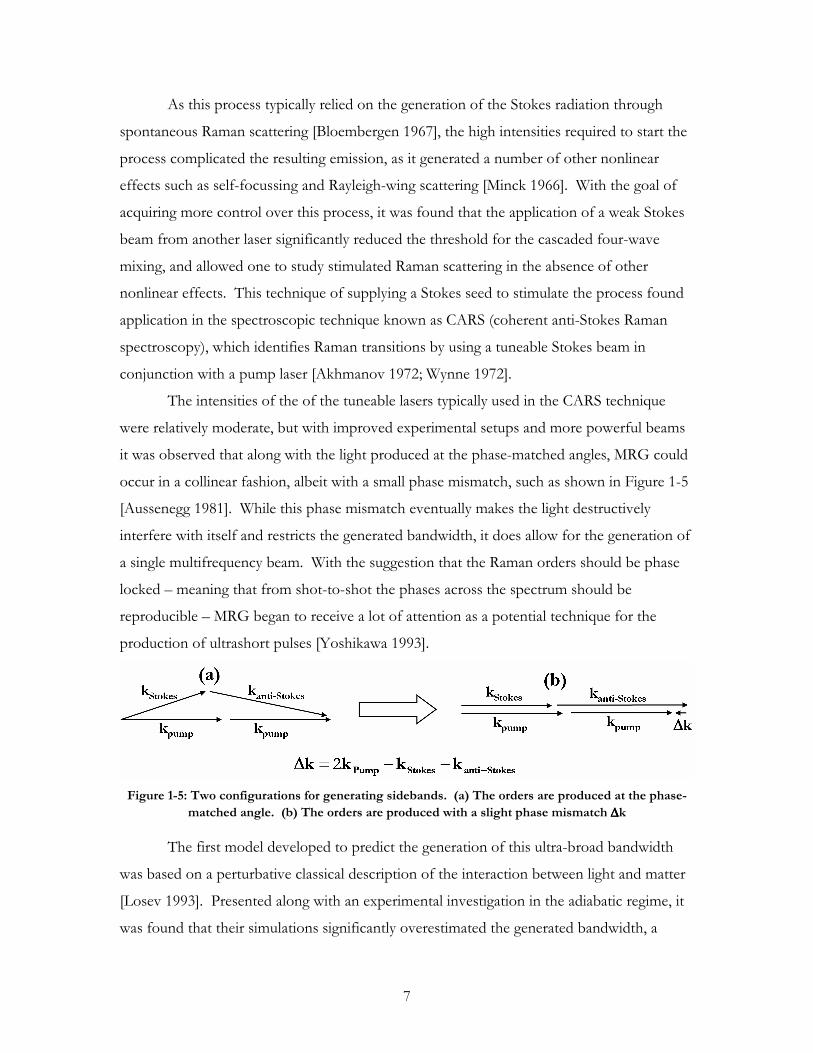
The intensities of the of the tuneable lasers typically used in the CARS technique
were relatively moderate, but with improved experimental setups and more powerful beams
it was observed that along with the light produced at the phase-matched angles, MRG could
occur in a collinear fashion, albeit with a small phase mismatch, such as shown in Figure 1-5
[Aussenegg 1981]. While this phase mismatch eventually makes the light destructively
interfere with itself and restricts the generated bandwidth, it does allow for the generation of
a single multifrequency beam. With the suggestion that the Raman orders should be phase
locked – meaning that from shot-to-shot the phases across the spectrum should be
reproducible – MRG began to receive a lot of attention as a potential technique for the
production of ultrashort pulses [Yoshikawa 1993].
Figure 1-5: Two configurations for generating sidebands. (a) The orders are produced at the phase-
matched angle. (b) The orders are produced with a slight phase mismatch ∆∆∆∆k The first model developed to predict the generation of this ultra-broad bandwidth
was based on a perturbative classical description of the interaction between light and matter
[Losev 1993]. Presented along with an experimental investigation in the adiabatic regime, it
was found that their simulations significantly overestimated the generated bandwidth, a
8
discrepancy which was attributed to the effect of diffraction. A two-dimensional simulation
confirmed this, demonstrating that the spatially-dependent Raman gain of a Gaussian beam
combined with the effect of diffraction would produce complex ring structures in the beam,
which in turn suppressed the generation of higher orders [Syed 2000]. This Raman
defocusing effect was studied experimentally soon afterwards, demonstrating a significant
increase in the beam diameter with increasing Stokes order, as well as the significant decrease
in generated bandwidth for more tightly-focused pump beams [Losev 2002a]. It is because
of this detrimental effect that many future experiments in MRG used hollow dielectric
waveguides (hollow fibres) filled with a Raman-active gaseous medium, confining the
generated spectrum in a single guided mode (therefore forcing it to be collinear as in Figure
1-5b), as well as increasing the interaction length from the diffraction limit to approximately
one meter [Nazarkin 1999; Sali 2004].
With a solid theoretical model behind them, investigations immediately ensued into
the possibility of conducting MRG with shorter pulses, which would allow for higher
intensities and therefore increasing the strength of the nonlinear interaction. While it was
found that the generated bandwidth was even more sensitive to dispersion in the transient
regime as compared to the adiabatic [McDonald 1994], it was also predicted that the
bandwidth could be enhanced by a factor of 1.4 in the case of zero dispersion [Losev 1996].
As attractive as this enhancement was, the experimental difficulties in producing two
ultrafast laser pulses separated by a relatively small frequency shift delayed efforts to study
this regime until recently [Losev 2002b].
In parallel with the classical description of MRG, an alternative approach based in
the density matrix formalism of the Maxwell-Bloch equations suggested the exciting
possibility that this multifrequency beam could spontaneously generate bright few-cycle
solitons. These static solutions for the electric field result in a pulse containing many Raman
orders that propagate at the same group velocity, due to a balance between the nonlinear,
frequency-dependent effect of MRG and the linear effect of dispersion [Kaplan 1994]. The
observation of these solitons would be a major advance in the field of ultrafast lasers, partly
because the complicated phase-correction techniques typical of other few-cycle schemes
would be unnecessary, but predominantly because it has been predicted that these pulses
would have durations as short as 200as – an order of magnitude shorter than anything that
had been observed at the time. As such, these stationary solutions received considerable

9
theoretical attention in the coming years in the steady-state regime [Kaplan 1996; Yavuz
2000] and in systems that can demonstrate negative dispersion [Nazarkin 1999b]. Soliton
formation has also been studied in the transient regime, however it is instead each order that
breaks into a soliton train [McDonald 1995], as opposed to multiple orders becoming locked
into a single train of solitons travelling at a specific group velocity.
Using the same density-matrix formalism, the simulations of Harris & Sokolov
(1997) demonstrated the generation of bandwidths that were comparable to those predicted
by Losev & Lutsenko (1993), however their subsequent experimental investigations achieved
significantly more conversion than previously reported especially into the anti-Stokes orders
[Sokolov 2000]. Indeed, further development of their technique resulted in the most
impressive demonstration of MRG to date, producing over 200 Raman orders using a
combination of two Raman-active media and three pump pulses [Yavuz 2003]. In the
course of their investigations they were also able to demonstrate the synthesis of ultrashort
pulses by properly phasing the distinct Raman orders, first producing a pulse train consisting
of 2fs pulses by using a series of prisms and delay lines overlap the orders in time [Sokolov
2001], and eventually generating a train of 1.6fs pulses using a liquid-crystal spatial light
modulator to adjust their phases [Shverdin 2005].
While these constitute the shortest pulses ever produced with MRG, their main
drawback lies in the duration of the pump pulses as compared to the Raman period. As the
Raman period dictates the separation between consecutive pulses and the duration of the
pump dictates the number of these pulses generated, the 11fs vibrational period of the
deuterium they used would produce approximately one million pulses within their 10ns
pump pulses. Each ultrashort pulse would then contain an average energy of ~100nJ,
minimizing their usefulness as an experimental tool. Soon after the initial adiabatic
demonstration however, pulses of a similar duration but an order of magnitude more energy
were obtained by another group, who instead of working with ns pumps were using
impulsive excitation to generate ultrashort pulses [Zhavoronkov 2002].
Intrinsically, impulsive MRG is less suitable for the generation of ultrashort pulses
than continuum generation or even adiabatic MRG, as the interaction between MRG and
self-phase modulation (SPM) leads to a suppression of both the high-frequency wing
characteristic of SPM, and the high order anti-Stokes scattering characteristic of MRG [Korn
1998; Kalosha 2003]. It is with an alternative pump-probe setup that impulsive excitation

10
has a real advantage, where the relatively mature pump sources at ~10fs [Rauschenberger
2006], are used simply as a tool to excite a coherence in the system, and it is instead the
scattering of a probe pulse injected behind the impulsive pump that is of interest [Nazarkin
1999a]. This pump-probe scattering is qualitatively different than typical MRG, in that from
the point of view of the probe, the scattering is essentially a linear process as opposed to a
non-linear one [Wittmann 2000; Nazarkin 2002a]. That is, the impulsive pump provides the
two photons coupling the ground and excited state, and the probe only needs to supply the
third photon to scatter into its Stokes and anti-Stokes orders (see in Figure 1-1a for anti-
Stokes scattering). In this linear scattering regime, compression of the radiation into few-
femtosecond pulse trains required either the application of positive or negative group-
velocity dispersion (GVD), which could be accomplished by simply propagating the pulses
through a dispersive medium for positive GVD, or by using commercially available chirped
mirrors to supply negative GVD [Wittmann 2000; Wittmann 2001]. The symmetric nature
of this compression is a consequence of the FM-like modulation experienced by the probe,
which would periodically delay or advance the phase of the light (see Figure 1-2 for an
illustration of this modulation).
By reducing the duration of the probe to where it was shorter than a single molecular
oscillation, this technique was able to generate an isolated few-femtosecond pulse
[Zhavoronkov 2002]. With a phase modulation that is no longer periodic (as the probe only
exists for a fraction of the molecular oscillation), a more continuous spectrum is generated,
which analogous to continuum generation allows the formation of a single pulse. In the
course of that particular experiment a pulse with a duration of 3.8fs and an energy of 1.5µJ
was synthesized. By utilizing the plasma-like dispersion in hollow fibres to match the group-
velocity of the probe to the original pump beam, even shorter pulses may be possible using
this technique [Nazarkin 2002b]. Another advantage of this technique is its scalability in
terms of the probe frequency – given sufficiently short probes in the mid-infrared and uv
regions of the spectrum, pulses of durations around 6fs and 2fs could be generated, which is
not currently possible with other short-pulse techniques [Kalosha 2003]. While this
operation in previously inaccessible frequency regimes is a major step forward for ultrafast
science, the generated probes are still an order of magnitude less energetic than comparable
continuum techniques. As there must be some way to disentangle the probe beam from the

11
pump, it is very difficult to apply in the range where higher-energy probes are most available
– the 700-900nm range of the Ti: Sapphire lasers used to generate the impulsive pump beam.
Herein lies the advantage of a symmetric, transient pumping scheme with laser pulses
of durations on the order of hundreds of femtoseconds. By selectively irradiating the
medium with two pump pulses tuned to the Raman resonance, one can take full advantage
of the high energies available in Ti:Sapphire pulses by avoiding the strong SPM characteristic
of the impulsive regime, while producing a much shorter pulse train than is possible with
nanosecond pumping. The first demonstration of transient MRG was in 2002 using a
KGd(WO4)2 crystal (KGW), as the Raman-active medium [Losev 2002b]. Having earlier
predicted that the generated bandwidth is maximized with the ratio of the pulse length to the
dephasing time [McDonald 1994], the 1.3ps dephasing time of KGW made it very attractive
as compared to the nanosecond dephasing time of many gasses. However, it was found that
the sensitive nature of transient pumping to dispersion dominated the possible enhancement
from the short dephasing time, and as such only a few orders were generated. Furthermore,
the short pumps experienced a significant amount of self-phase modulation as they passed
through the crystal, limiting the number of orders generated as compared to stretched pulses
[Losev 2002b]. The detrimental effects due to the solid medium were remedied by
conducting transient MRG in a hollow fibre filled with a Raman-active gas, where the
generated orders spanned at least the wavelength range from 800nm to just below 300nm,
from which it is predicted a 1fs pulse can be synthesized assuming perfect phase
compensation [Sali 2004]. Further investigations confirmed the detrimental effect of SPM as
the growth of the bandwidth with pressure halted with the onset of self-phase modulation,
and also demonstrated the overall bandwidth generated with different media were
approximately the same, even if the number of orders are different [Sali 2005].
With the demonstration that bandwidths spanning the visible spectrum can be
obtained in the transient regime, experimental efforts are being directed towards optimizing
and compressing this bandwidth. The investigations presented in this report are the most
recent efforts of our group towards generating high-energy ultrashort pulses in the transient
regime of MRG. Detailed in the following chapters is the culmination of my efforts towards
these goals to date, including a theoretical discussion of the equations pertaining to the
classical description of MRG, a computer model based on those equations aimed at
explaining the results obtained in the laboratory, the first experimental demonstration of

12
transient MRG in SF6 using our two-colour laser system, the scaling of this effect with
intensity as reported in Turner et al (2006), the most recent results of its behaviour with
pressure in a narrow hollow fibre, and some concluding remarks discussing the future
directions of this research.

13
2. Theory The theoretical treatment of Losev & Lutsenko (1993) provides a good starting point for
understanding the MRG process. A relatively intuitive classical description of MRG, it
provides much insight into the predominant mechanisms for the generation of multiple
orders, and as well benefits from a parallel and detailed description in the text Nonlinear
Optics [Boyd 2003]. §2.1 will describe in detail how to arrive at the equations in Losev &
Lutsenko (1993) by drawing upon the discussion in Nonlinear Optics from chapters 1, 2, and
especially 10. After concluding with the general equations in §2.1.4, two characteristic
behaviours of MRG – the Bessel-function character of the sidebands and an estimate of the
total bandwidth – will be described drawing on a variety of resources. The discussion will
then conclude with a description of the program developed to try and model the
experimental results.
2.1. Classical description
When an electric field ),(~
tzEρ
is incident upon a molecule, the electronic and nuclear
response of this molecule creates a polarization field ),(~
tzpρ
through its polarizability α
(the tilde denotes a term that is rapidly-varying). If the driving electric field is much weaker
than the atomic field cmstatvoltE atom /* 7102=ρ
mV /* 11106= , the molecule’s
response can be described using a perturbative technique, where the polarization is related to
the nth power of ),(~
tzEρ
through an nth-order tensor )( nχ . In an isotropic medium, this
tensor nature is suppressed and the polarization can be expressed as
( )433221 EOtzEtzEtzEtzp~
),(~
),(~
),(~
),(~ )()()( +++= χχχ [Eq. 2-1]
When discussing nonlinear effects due to this polarization, any that are related to the cube of
the electric field will be referred to as third-order or )( 3χ (chi-3), nonlinearities. Note that
( )nxO is meant to stand for “terms in x to the power of n and higher”, and the vector
notation has been dropped for clarity.
2.1.1. Driving Force and Molecular Motion
For the present derivation, consider the response of a vibrationally Raman-active diatomic
molecule to a linearly polarized pump beam. The polarization field due to a single molecule

14
is given by its polarizability α through the relation
),(~
),(),(~ tzEtztzp ⋅=α [Eq. 2-2]
Note that for this derivation the medium is assumed to be isotropic (which corresponds to
our experimental case of SF6), and as such α is simply a scalar quantity. The key
assumption in this derivation is that the polarizability should only be weakly dependent on
the internuclear separation, as it is mainly a result of the electronic configuration of the
molecule. Written to first order, the polarizability thereby has the form
( ) ),(),( tzqqtzqq⋅∂∂+= = 0
0 ααα [Eq. 2-3]
where q is the vibrational coordinate given by
),(~),( tzqqtzq += 0 [Eq. 2-4]
as in Figure 2-1. This leads to a polarization of
),(~),(~
),(~),(),(
~),(~
tzptzp
tzEtzqq
tzEtzp
NonlinearLinear
+=
∂∂
+== 0
0
αα
[Eq. 2-5]
It will become convenient later to drop the linear part of the polarization, as it does not
directly affect the MRG process (but does play a role through the index of refraction).
Figure 2-1: Vibrating diatomic molecule
Now, assume that the molecule acts like a simple harmonic oscillator with a single
resonant frequency Vω , reduced nuclear mass m , and damping constant γ . Its motion
from equilibrium q~ will follow the equation
m
tzFq
t
q
t
qV
),(~
~~~
=+∂
∂+
∂
∂ 2
2
2
2 ωγ [Eq. 2-6]

15
where the applied force ),(~
tzF acts along the vibrational coordinate q . This force, which
is generated by the electric field, can be found by taking the gradient of the work needed to
create the polarization ),(~ tzp . Under the dipole approximation this can be written as
⋅−
∂∂
−=∂∂
−= ),(~
),(~),(~
tzEtzpqq
WtzF
2
1 [Eq. 2-7]
where the angular brackets denote the time average over an optical period. By substituting
the expressions for ),(~ tzp and ),( tzα , this reduces to
),(~
),(~
tzEq
tzF 2
02
1
∂∂
=α
[Eq. 2-8]
. In typical experimental designs, MRG is produced by starting with two pump beams
tuned to the Raman resonance, where VStokespump ωωω ≈Ω=− as in Figure 1-1. However
it is useful to consider the case of four input fields of comparable intensity to facilitate the
generalization of this effect. Therefore, consider a driving field that consists of a pump
beam of index 0, a Stokes beam of index -1, an anti-Stokes beam of index +1, and a second-
order Stokes beam of index -2. The notation and form of the electric field will be slightly
modified from Boyd’s description to help ease the transition to the notation of Losev &
Lutsenko (1993), which was used to develop the computational model. Note that while the
following equations are quite involved, the important information can simply be found by
looking at the indices of the amplitude and phase terms to get a sense of what orders are
involved.
Each component of this four-component electric field is taken to be of the form
( )[ ] ( )[ ]( )tzkiEtzkiEtzE NNNNNNN ωω −+−−= expexp),(~ *
2
1 [Eq. 2-9]
where the * denotes the complex conjugate. The frequencies are spaced approximately by
the Raman frequency such that Ω⋅+= NN 0ωω , where 0ωω <<≈Ω V , and the
wavevector cnk NNN ωω ⋅= )( . The four-colour electric field can then be written as
( )[ ] ( )[ ]( )( )[ ] ( )[ ]( )( )[ ] ( )[ ]( )( )[ ] ( )[ ]( )tzkiEtzkiE
tzkiEtzkiE
tzkiEtzkiE
tzkiEtzkiEtzE
222222
111111
000000
1111112
−−−−−−
−−−−−−
−+−−+
−+−−+
−+−−+
−+−−=
ωω
ωω
ωω
ωω
expexp
expexp
expexp
expexp),(~
*
*
*
*
[Eq. 2-10]

16
where the amplitudes are approximately equal 2101 −− ≈≈≈ EEEE . Note that in
general the index of refraction is a nonlinear function of the frequency. In a more compact
notation that will be often be used in this discussion, the electric field can be rewritten as
( )[ ] ( )[ ]( )[ ] ( )[ ]
c.c.
tzkiEtzkiE
tzkiEtzkiEtzE
+
−−+−−+
−−+−−=
−−−−−− 222111
0001112
ωωωω
expexp
expexp),(~
[Eq. 2-11]
where the complex conjugate is denoted as c.c. The square of this field is then
( )[ ] [ ] [ ]( )[ ][ ] [ ]( )[ ] [ ] [ ]( )[ ]
[ ] [ ]( )[ ][ ] [ ]( )[ ] [ ] [ ]( )[ ]
[ ] [ ]( )[ ] ( )[ ][ ] [ ]( )[ ] [ ] [ ]( )[ ][ ] [ ]( )[ ][ ] [ ]( )[ ] [ ] [ ]( )[ ]
[ ] [ ]( )[ ] [ ] [ ]( )[ ]( )[ ] [ ] [ ]( )[ ]
[ ] [ ]( )[ ] [ ] [ ]( )[ ][ ] [ ]( )[ ]
[ ] [ ]( )[ ] [ ] [ ]( )[ ][ ] [ ]( )[ ] ( )[ ][ ] [ ]( )[ ] [ ] [ ]( )[ ][ ] [ ]( )[ ] c.c.EtzkkiEE
tzkkiEEtzkkiEE
tzkiEtzkkiEE
tzkkiEEtzkkiEE
tzkkiEEE
tzkkiEEtzkkiEE
tzkkiEEtzkiE
tzkkiEEtzkkiEE
tzkkiEEtzkkiEE
EtzkkiEE
tzkkiEEtzkkiEE
tzkiEtzkkiEE
tzkkiEEtzkkiEE
tzkkiEEE
tzkkiEEtzkkiEE
tzkkiEEtzkiEtzE
++⋅−−−−+
⋅−−−−+⋅−−−−+
−−+⋅+−+−+
⋅+−+−+⋅+−+−+
⋅−−−−++
⋅−−−−+⋅−−−−+
⋅+−+−+−−+
⋅+−+−+⋅+−+−+
⋅−−−−+⋅−−−−+
+⋅−−−−+
⋅+−+−+⋅+−+−+
−−+⋅+−+−+
⋅−−−−+⋅−−−−+
⋅−−−−++
⋅+−+−+⋅+−+−+
⋅+−+−+−−=
−−−−−−−
−−−−−−
−−−−−−−−−
−−−−−−
−−−−−−−
−−−−−−
−−−−−−−−−
−−−−−−
−−−−−−
−−−−−−
−−−−−−
−−−−−−
2
2121212
020202121212
22
2
2121212
020202121212
212121
2
1
010101111111
21212111
2
1
010101111111
202020101010
2
0101010
202020101010
0020101010
212121111111
010101
2
1
212121111111
01010111
2
1
2
22
22
22
224
ωω
ωωωω
ωωω
ωωωω
ωω
ωωωω
ωωω
ωωωω
ωωωω
ωω
ωωωωωωω
ωωωω
ωω
ωωωωωωω
exp
expexp
expexp
expexp
exp
expexp
expexp
expexp
expexp
exp
expexp
expexp
expexp
exp
expexp
expexp),(~
*
**
*
**
**
*
**
*
[Eq. 2-12]
While this is a pretty complicated expression, it can be simplified under the
assumption that the medium is dispersionless. In that case 0nn =)(ω , and both the
frequencies and wavevectors are separated by a constant value: Ω=− −1ii ωω and
κ=− −1ii kk . It can be further simplified by removing all the terms in the complex

17
conjugate with positive frequencies, and sending all terms with negative frequencies into the
complex conjugate. ),(~
tzE 2 can then be grouped as follows:
( )[ ] ( )[ ]( )[ ] ( )[ ]
[ ] [ ]( )[ ] [ ] [ ]( )[ ][ ] [ ]( )[ ] [ ] [ ]( )[ ][ ] [ ]( )[ ] [ ] [ ]( )[ ]
( )[ ]( ) ( )[ ]( ) ( )[ ] ..exp
exp
exp
expexp
expexp
expexp
expexp
expexp
),(~
***
**
*
cctziEEEEEE
tziEEEE
tziEE
tzkkiEEtzkkiEE
tzkkiEEtzkkiEE
tzkkiEEtzkkiEE
tzkiEtzkiE
tzkiEtzkiE
EEEEtzE
+Ω−−+++
Ω−−++
Ω−−+
⋅+−+−+⋅+−+−+
⋅+−+−+⋅+−+−+
⋅+−+−+⋅+−+−+
−−+−−+
−−+−−+
+++=
−−−
−−
−
−−−−−−−−−
−−−−−−
−−−
−−−−−−
−−
κ
κ
κ
ωωωωωωωω
ωωωω
ωω
ωω
211001
2011
21
212121202020
101010212121
111111010101
222211
21
002011
21
22
21
20
21
2
2
222
332
22
22
22
2222
2222
4
[Eq. 2-13] As Vω≈Ω , the terms that oscillate at this frequency will dominate the equation of
motion (last line in [Eq. 2-13]), and so the other non-resonant terms can be dropped.
Furthermore, as Ω is much smaller than any optical frequency, these resonant terms will
essentially be constant over the time average, and as such we can simply drop the angular
brackets. The driving force is then
( ) ( )[ ] ..exp
),(~
),(~
*** cctziEEEEEEq
tzEq
tzF
+Ω−−++
∂∂
=
∂∂
=
−−− κα
α
211001
0
2
0
4
1
2
1
[Eq. 2-14]
Given this driving term, assume a solution to [Eq. 2-6] of the form
( )[ ] ( )[ ]tzizqtzizqtzq Ω−⋅+Ω−−⋅= κκ exp)(exp)(),(~ * [Eq. 2-15]
and insert this into the equation. The result is
mtzFtzqtzqitzq V ),(~
),(~),(~),(~ =+Ω+Ω− 22 2 ωγ [Eq. 2-16]
and yields a total solution to the molecular motion of the form
( ) ( )[ ] ..exp),(~***
cctzii
EEEEEE
qmtzq
V
+Ω−−Ω+Ω−
++
∂∂
= −−− κγω
α24
122
211001
0
[Eq. 2-17]

18
2.1.2. Nonlinear Polarization and Resulting Field
With the molecular motion accounted for, the total nonlinear polarization – or the number
of molecules N times the single molecule polarization in [Eq. 2-5]:
),(~),(~),(~),(
~tzEtzq
qNtzpNtzP NLNL
0
∂∂
=⋅=α
[Eq. 2-18]
is found to be of the form:
( )( ) ( )[ ]( )[( ) ( )[ ]( )( ) ( )[ ]( )( ) ( )[ ]( )( ) ( )[ ]( )( ) ( )[ ]( )( ) ( )[ ]( )( ) ( )[ ]( ) ]..exp)(
exp)(
exp)(
exp)(
exp)(
exp)(
exp)(
exp)(
),(~
*
*
*
*
cctzkiEzq
tzkiEzq
tzkiEzq
tzkiEzq
tzkiEzq
tzkiEzq
tzkiEzq
tzkiEzq
qNtzPNL
+Ω−−−−⋅+
Ω−−−−⋅+
Ω−−−−⋅+
Ω+−+−⋅+
Ω−−−−⋅+
Ω+−+−⋅+
Ω+−+−⋅+
Ω+−+−⋅
∂∂=
−−−
−−−
−−−
−−−
222
111
000
222
111
111
000
111
0
ωκ
ωκ
ωκ
ωκωκ
ωκωκ
ωκ
α
[Eq. 2-19]
Notice the affect of q and q* on the frequencies, where they either increase or decrease the
frequency by Ω , and the new frequency components generated at Ω+= 12 ωω and
Ω−= −− 23 ωω .
To determine the resulting electric field, the optical wave equation
),(~
),(~
),(~
tzPtc
tzEtc
tzEρρρ
2
2
22
2
2
41
∂
∂−=
∂
∂+×∇×∇
π [Eq. 2-20]
must be solved, where
),(~
),(~
),(~
tzEtzEtzEρρρ
2∇−
⋅∇∇=×∇×∇ [Eq. 2-21]
is often approximated as
),(~
),(~
tzEtzEρρ
2−∇≈×∇×∇ [Eq. 2-22]
(since there is typically only a very small component of the electric field pointing in the
direction of propagation – for the plane waves being considered,
⋅∇∇ ),(
~tzE
ρ vanishes
identically). This equation reduces to:
19
),(~
),(~
),(~
tzPtc
tzEtc
tzE NL
ρρρ2
2
22
2
2
2 41
∂
∂−=
∂
∂+∇−
π[Eq. 2-23]
where again, only the contributions due to the nonlinear polarization are being investigated –
the linear polarization affects the field indirectly through the index of refraction. Equating
terms that oscillate at a particular frequency, for example at 0ωω = :
( )[ ]( )
( )[ ]( )
[ ] ( )[ ]( )..exp)()(
..exp
..exp
* cctzkiEzqEzqtqc
N
cctzkiEtc
n
cctzkiEz
+−−+∂
∂
∂∂
−=
+−−∂
∂+
+−−∂
∂−
− 00112
2
0
2
0002
2
2
20
0002
2
4ω
απ
ω
ω
[Eq. 2-24]
which after differentiation becomes:
[ ]( ) [ ]( ) [ ]( )
[ ]( )
[ ] ( )[ ]( )..exp)()(
..exp
expexpexp
* cctzkiEzqEzqqc
N
cctzkiEc
n
tzkiEktzkiz
Eiktzki
z
E
+−−+
∂∂
=
+−−−
−−+−−∂
∂+−−
∂
∂−
− 0011
0
2
20
0002
20
20
0002000
00002
02
4
2
ωαωπ
ωω
ωωω
[Eq. 2-25]
A typical approximation when solving this equation is the slowly-varying envelope
approximation
z
Ek
z
E
∂
∂<<
∂
∂ 002
02
[Eq. 2-26]
which says that the envelope is evolving on a length scale much longer than a wavelength.
This, along with the fact that cnk ω⋅≡ , allows one to get rid of the first, third, and fourth
terms on the left-hand side, leading to the coupled amplitude equation that describes MRG
( )11
0
00 2EzqEzq
cn
i
z
E)()( *+−=
∂
∂−
ωπ [Eq. 2-27]
2.1.3. Dispersion
Now, to include dispersion into this model the various phase contributions from the
wavevector k need to be accounted for. This could have been done from the beginning, but
would have complicated the expressions even further. To put these contributions back in,

20
one can simply multiply each amplitude E and *E by a factor of )exp( ik− and
)exp( ik+ respectively as in [Eq. 2-9], and relax the condition of a dispersionless medium so
that 11 −− −≠− mmnn kkkk when mn ≠ (however, it is still true that Ω=− −1nn ωω ).
For example, the equation for the molecular motion [Eq. 2-17] would become
( )[ ](( )[ ]( )[ ])zkkEE
zkkEE
zkkEE
iqmtzq
V
2121
1010
0101
22
02
1
4
1
−−−−
−−
−−+
−−+
−−⋅
Ω+Ω−⋅
∂∂
=
exp
exp
exp
),(~
*
*
*
γωα
[Eq. 2-28]
and the coupled amplitude equation [Eq. 2-27] would be
( )
( ) ( )( )zikEtzqzikEtzq
qcn
iNzik
z
E
1111
00
00
0 2
−+−⋅
∂∂
−=−∂∂
−− exp),(~exp),(~
exp
*
αωπ [Eq. 2-29]
or
[ ]( ) [ ]( )( )zkkiEtzqzkkiEtzq
qcn
iN
z
E
011011
00
00 2
−−+−−⋅
∂∂
−=∂∂
−− exp),(~exp),(~ *
αωπ[Eq. 2-30]
2.1.4. Generalization
The generalization of these equations to an arbitrary number of fields is relatively
straightforward. By simply summing over the field components, the equation for the
molecular motion and the coupled amplitude equation become:
( )
Ω+Ω−
∆−⋅
∂
∂=
∑∞
−=−
γωα
i
ziEE
qmtzq
V
Mnnnn
24
122
1
0
exp
),(~
*
[Eq. 2-31]
( ) ( )( )ziEtzqziEtzqqcn
iN
z
Ennnn
n
nn111
0
2++− ∆−+∆
∂∂−
=∂
∂exp),(~exp),(~
)(
*αω
ωπ[Eq. 2-32]
21
where M
−
Ω= 10ω rounded up to the nearest integer and 1−−=∆ nnn kk . This
definition of M allows the summation to include all combinations of positive frequencies
whose difference equals the separation Ω .
2.2. Characteristics of MRG These coupled differential equations describing MRG pose an incredible challenge to those
looking for a complete analytical solution, especially considering that experiments have
demonstrated the generation of over 200 field components [Yavuz 2003]. As a result, most
of the published literature trying to describe this effect present a numerical model when
discussing particular experimental results, whether in the steady-state [Losev 1993],
impulsive [Kalosha 2003], or transient regimes [Sali 2005]. However as in most areas of
physics, much physical insight can still be gained by considering various limiting cases of
these equations – of particular importance is the demonstration of 1) the Bessel-function
character of the Raman orders as they propagate through the system, and 2) an estimate of
the total number of orders one would expect with intensities on the same order of
magnitude.
2.2.1. Bessel-Function Character of MRG
This discussion is based primarily on the report by Harris & Sokolov (1998), which
investigated MRG in the steady-state regime using a two-colour pump at 0ω and 1−ω .
While a density matrix formalism involving the Maxwell-Bloch equations are used to
describe this process as opposed to the classical argument, the resulting equations (after
some simplifications), are formally equivalent. For example, equation #6 in their report:
( )11 +− +−=∂
∂qabqabq
qEEi
z
E ~~~~~
*ρρβ [Eq. 2-33]
looks like [Eq. 2-32] by collecting the constants from [Eq. 2-32] into a single constant β and
by making the substitution βωβ ⋅= qq in [Eq. 2-33]. One must also assume that abρ~ plays
the role of ),(~ tzq .
The key realization is that the coupled amplitude equation of Eq. 2-3 has a parallel in
the Bessel function identity

22
( ))()()(
xJxJx
xJqq
q
112
1+− −=
∂
∂ [Eq. 2-34]
[Spiegel 1999]. Following this, the authors assume a dispersionless medium in the limit of
weak excitation, such that only a limited bandwidth is produced and that the molecular
excitation ),( tzq is constant throughout the medium. This leads to the approximations
that ),( tzq can be described by a simple phase ( )00 φiqtzq exp),( ∝≡ and all of the
generated frequencies 0ωω ≈n , which together reduce [Eq. 2-32] to
( )1010 +− +−=∂
∂nn
n EqEqiz
E *β [Eq. 2-35]
where β is a positive and real constant. The authors then assume a solution of the form
[ ]( )[ ] [ ]( ) ..)(exp)(
)(exp)()(
cczJniE
zJniEzE
n
nn
++⋅−+
−=
+− γπφγπφ
101
00
120
20 [Eq. 2-36]
where γ is a phenomenological constant taken to be real and positive. To motivate this
choice of solution, a few issues concerning the initial condition
( ) ..)exp()(exp)(),(~
cctiEtiEtE ++= −− 1100 0002 ωω need to be considered:
1. The flow of radiation should depend on the initial values of both pumps
2. Of the ordinary Bessel functions )( xJ n , only )( xJ 0 has an initial value
that is non-zero, and so each pump field ),( tzE 0 and ),( tzE 1− must be
multiplied by the appropriate Bessel function.
3. The initial values of the pumps do not depend on the phase of the molecular
motion 0φ , however any radiation scattered from other fields should depend
on this factor, as the light must scatter from ),(~ tzq .
While these considerations do not require the inclusion of 2π− in the phase terms, this
will become important later in the derivation. Substituting [Eq. 2-36] into [Eq. 2-35]:
[ ]( ) ( )
[ ] [ ]( ) ( )
..
)()(exp)(
)()(exp)(
)(
cc
zJzJniE
zJzJniE
z
zE
nn
nnn
+
−+⋅−+
−−=
∂
∂
+−
+−
2120
220
201
1100
γγπφγ
γγπφγ
[Eq. 2-37]

23
which can be rearranged to form
[ ]( )[
[ ] [ ]( ) ]
[ ]( )[
[ ] [ ]( ) ]..
)(exp)(
)(exp)(
)(exp)(
)(exp)()(
cc
zJniE
zJniE
zJniE
zJniEz
zE
n
n
n
nn
+
+⋅−+
−−
+⋅−+
−=∂
∂
+−
+
−
−
γπφ
γπφγ
γπφ
γπφγ
201
100
01
100
120
202
120
202
[Eq. 2-38]
Note the mismatch between the index of the Bessel functions and the index of the
exponentials. This can be adjusted by pulling out an appropriate phase from the
exponentials:
( ) ( ) [ ] [ ]( )[
[ ]( ) ]
( ) ( ) [ ] [ ]( )[
[ ]( ) ]..
)(exp)(
)(exp)(expexp
)(exp)(
)(exp)(expexp)(
cc
zJniE
zJniEii
zJniE
zJniEiiz
zE
n
n
n
nn
+
⋅−+
+⋅−−−
⋅−+
−⋅−−=∂
∂
+−
+
−
−
γπφ
γπφπφγ
γπφ
γπφπφγ
201
1000
01
1000
20
12022
20
12022
[Eq. 2-39]
After comparing this to [Eq. 2-36], one can rewrite this as
( ) ( )
( ))()(
)(exp)(exp)(
* zEqzEqi
zEii
zEii
z
zE
nn
nnn
1010
101022
+−
+−
+−=
−−−=∂
∂
β
φγ
φγ
[Eq. 2-40]
where βγ 2= . Thus, in the limit of weak excitation, the equations for individual field
components is a sum of two Bessel functions as shown in [Eq. 2-36].
2.2.2. Components of comparable intensity
To make short pulses one needs a large bandwidth, and so the question of how many orders
can be produced (and therefore bandwidth), is natural to consider. A simple expression can
be found using the approximations described in §2.2.1, however Losev & Lutsenko (1993)
address this question with relatively few approximations, and as such can discuss the
behaviour of MRG even beyond the limit of weak excitation.
To compare directly to the formalism of Losev & Lutsenko (1993), assume again
that the pump is a two-colour beam at 0ω and 1−ω , but that it is exactly on resonance so
that Vωωω =Ω=− −10 . Adjust the phase of molecular motion so that ),(~ tzqiQ ⋅≡ ,

24
normalize the field amplitudes )( zE n such that E
zEA nn
)(
)(
00
≡ , and define the irradiance
(hereafter to be referred to as the intensity), as zEzEzI *nnn )()()( ≡ . With these
definitions, equations [Eq. 2-31] and [Eq. 2-32] become equations (1) and (2) in the
manuscript:
( )∑∞
−=− ∆−=
Mnnnn ziAAIQ exp)( *
10 0α [Eq. 2-41]
[ ] [ ]( )ziQAziAQz
Annnn
nn ∆−∆−=∂
∂−++ expexp*
111
0ωω
β [Eq. 2-42]
where the real and positive coefficients 0
4
1
∂∂
≡qm V
αγω
α and 0
0
∂∂
≡qcn
N
n
αωωπ
β)(
.
With this revised notation, consider again the case of weak excitation, where it was found
that the field could be described using Bessel functions, but this time in the context of [Eq.
2-41] and [Eq. 2-42]. One property of ordinary Bessel functions )( xJ n is that the number
of orders n with approximately the same amplitude is given by twice the argument x . As
this gives a direct measure of the number of fields generated in MRG, the argument of these
functions should in turn provide an estimate of the generated bandwidth, where
( ) V1 - Fields of # ωω ⋅≈∆ . In the discussion of §2.2.1, the arguments of the Bessel
functions included the factor γ , which itself was twice the value of the constant in the
coupled amplitude equation. Pulling the real constants from Q into zAn ∂∂ , one can
obtain the slightly modified coupled amplitude equation
[ ] [ ]( )ziQAziAQIz
Annnn
nn ∆−∆−=∂
∂−++ expexp)( *
111
0
0 0ωω
αβ [Eq. 2-43]
Within the assumptions of weak excitation and a dispersionless medium, the argument of the
Bessel functions is then
zIqmn
N
cz
V
⋅⋅
∂∂
= )( 02
0
2
0
0
0
αωω
γπ
γ [Eq. 2-44]
implying that the bandwidth (which is Vzωγ2≈ ), should increase linearly with distance,
pressure (N ), intensity, pump frequency, and the dephasing time of the molecular
vibrations ( γ1 ). Notice however that the bandwidth should not scale with the vibrational

25
frequency Vω , implying that it should be roughly the same between molecular species,
provided other molecular parameters are similar.
Relaxing the conditions that 0ωω =n and 0=∂∂ zzq )( , a general formula for the
number of components generated can be derived. As presented in Losev & Lutsenko
(1993), it can be shown with the approximation of zero dispersion that the parametric
growth rate ∫ ⋅≡z
dxQ0
βξ , which defines the strength of the MRG interaction, is
approximately equal to both the number of Stokes and anti-Stokes orders generated. As
well, with the assumption that the amplitudes nA fall off rapidly with increasing n such
that 021 →−
nAn as ∞−→ or Mn , ξ can be determined by considering the normalized
intensity ∑∞
−−=
1M nnAAJ * and the normalized polarizability amplitude ∑∞
− −=M nnAAS *
1 .
Through the significant manipulations described in Losev & Lutsenko (1993) these lead to
an expression for the parametric growth rate
( )
( )
∞
∞+∞
=
2
2
0
0
)(arctanhtanh
)(arctanh)(tanh
ln)(J
JBJ
B
V
V
ωω
ωω
ξ [Eq. 2-45]
where the limiting value of the intensity )(∞J tends toward
[ ]2001 )()()( JSJ −=∞ [Eq. 2-46]
This growth rate ξ is given as a function of the Raman Parameter B which, similar to the zγ
parameter in [Eq. 2-44], is related to the propagation distance, pressure, the initial intensity,
and the ratio between the pump frequency and the vibrational frequency
( )zIIqmn
N
cB
V
)()( 002
10
2
0
0
0
−+
∂∂
=α
ωω
γπ
[Eq. 2-47]
Note that again, the total bandwidth which is now given by Vξωω 2≈∆ is invariant with
respect to the Raman frequency Vω , as the parameter B is multiplied by 0ωωV in [Eq. 2-
45].
As shown in Figure 2-2, this expression for ξ will be approximately linear at low
values of B , but as the pressure, pump intensity, or propagation distance starts to become

26
large the process begins to saturate (see Figure 2-2). In the limiting case, the parametric
growth rate tends to the value
( ) ( )
∞=∞
20
)(arctanhcothln)(
JVωωξ [Eq. 2-48]
Note that this expression is only dependent on the initial relative strength of the two pumps
(in the expression for )(∞J ). This implies that the total possible bandwidth is only
dependent on the pump frequency and the relative strengths of the pump and Stokes beams
– all other factors such as the intensity, pressure, the properties of the molecule and the
propagation distance simply affect the rate at which one obtains this bandwidth.
Figure 2-2: Plot of the parametric growth rate as a function of the Raman parameter B . Note the initial linear behaviour and the subsequent saturation.
2.3. Computational model To help describe the observations of the experiment, a computational model describing
MRG was developed in Matlab. While the accuracy of the model is simply limited by the
level of complexity one chooses to include, for practical purposes the first attempt only
included the classical on-resonance description of Losev & Lutsenko (1993), which neglects
diffraction, population of the vibrational level, and the effects of other )( 3χ processes such
as self-phase modulation.
As both the Raman generation and dispersion can be described in the frequency
domain within the classical formalism, the electric field is treated as a single array in ω , even
when working in the transient regime where the pulses are short and the bandwidths large.
While this differs from the typical carrier-envelope treatment typical of models starting from
the Maxwell-Bloch equations, where each order is given a temporal envelope for a particular
carrier frequency Vn nωωω += 0 and the Raman generation is described in the temporal
domain [Sali 2005], it is in many ways similar to the recently developed single-field Maxwell-

27
Bloch model where a single array in t is used to describe the electric field [Kinsler 2005]. As
the classical description only requires one to work in the frequency domain, a single-field
description in frequency was chosen for this model as opposed to an adaptation of the
carrier-envelope technique.
To verify the validity of the computational model, the results for plane-wave
excitation in the zero dispersion limit were compared to those that are published [Losev
1993]. Using the same parameters as reported in the manuscript, the result of the
comparison is demonstrated in Figure 2-3. Although the agreement is generally good, there
is a discrepancy in the values of some of the troughs. It is believed that the spatial resolution
in z is limiting the agreement, however within the resources of the PC that was used this
could not be enhanced further. They are close enough however that it was expected the
essence of MRG had been captured in the program, and that while it may not give an exact
solution, a qualitative discussion should be feasible.
Figure 2-3: Comparison of the program to published results. (a) Figure 4b in Losev & Lutsenko (1993). (b) Superposition of the simulation with the spectrum in (a)
For clarity, the simulation is presented again in Figure 2-4a. Note the generation of a
bandwidth that, within an order of magnitude of the peak, contains ~31 Raman orders. This
corresponds well to the predicted analytical value of 352 =ξ . Qualitatively there are two
important features of this spectrum aside from the generated bandwidth – the first is the
large number of anti-Stokes orders generated compared to the Stokes, which may be a result
of the frequency dependence of the coupled amplitude equation (for the parameters chosen
the Raman order at an index of -20 is at a frequency of 215THz, whereas the Raman order at
an index of +30 is four times as large at 1095THz). The second feature of interest is that
while there are more anti-Stokes orders generated, the Stokes orders are generally more
intense. These higher intensities is a consequence of the parametric nature of MRG – to

28
generate an anti-Stokes photon, one must also generate a Stokes photon, which implies that
the flow of energy from the two pumps to higher frequencies must be matched by a flow of
energy to lower frequencies. This should not to be confused with a statement of the form
“each order of anti-Stokes must be matched by a corresponding Stokes order”, which is not
true – Figure 1-1a demonstrates how a second-order anti-Stokes photon can be generated by
converting pump photons into only first-order Stokes photons. In that case, one pump
photon absorbed an energy Vωη2 by forcing two pump photons to lose an energy of Vωη ,
thereby conserving energy.
Figure 2-4: Resulting spectrum from on-resonance excitation with zero dispersion. (a) Intensity spectrum of Raman orders. (b) The sign of the amplitude for each order: note the
regular phase jumps of
Another insight that can be gained from the simulation is the fact that the
dispersionless MRG spectrum does not spontaneously produce short pulses. This is
illustrated in Figure 2-5, where a numeric fast Fourier transform of the spectrum was used to
produce a temporal profile in parts (a) and (b), however in part (a) the phase was left
unchanged and in (b) it was assumed that the phases were perfectly compensated, and so of
the same sign across the entire spectrum. The broad temporal profile observed in Figure 2-
5a is therefore a result of the regular phase jumps of π apparent in Figure 2-4b, where the
amplitudes of the Raman orders flip back and forth from positive to negative across the
spectrum. Both the spectrum and the signs determined in this model are consistent with the
model of Kalosha & Herrmann (2000), with slight deviations similar to those found when
comparing the results to Losev & Lutsenko (1993) in Figure 2-3.

29
Figure 2-5: Fast Fourier transform of the spectrum in Figure 2-4a. (a) The phase of the spectrum includes the jumps of as in Figure 2-4b. (b) The phase is assumed to be flat across the spectrum.

30
3. Experimental Apparatus The optical setup in general follows the block diagram of Figure 3-1. In brief, a broad-
bandwidth pulse is generated in the laboratory of Dr. Joseph Sanderson, where it is stretched
to ~1ns and delivered via single mode fibre to the laboratory of Dr. Donna Strickland. This
pulse is amplified using a dual-wavelength regenerative amplifier [Zhang 2000], and then
further amplified using a dual-wavelength multipass amplifier [Xia 2002]. The pulses are
then compressed and focussed into a hollow dielectric waveguide filled with SF6 gas. The
resulting MRG spectrum is then sent to two spectrometers simultaneously to record the
ultra-broad bandwidth.
Figure 3-1: Block Diagram of the Experimental Apparatus
Sulphur hexafluoride was chosen as the Raman-active medium due to a number of
qualities that made it particularly suitable for study with this system. Primarily, its Raman-
active 23THz A1g vibrational mode [Herzberg 1945], was well within the range of the two-
colour amplifiers, which in the past have been used to generate colours as far apart as
~40THz [Xia 2003]. A secondary benefit of this small vibrational frequency (small
compared to simple diatomic molecules), is that it should result in a relatively large pulse
spacing of about 43fs according to Fourier theory. With pump envelopes of a few hundred
femtoseconds, the bulk of the energy should be contained in only a few ultrashort pulses
after compression. The second main advantage of SF6 is its vibrational dephasing time of
6.6ps [Everall 1987]. The gain in transient MRG has been found to depend on the ratio of
the pulse duration to the dephasing time [McDonald 1994], and as such we should be able to
get efficient generation with pulse durations of a few hundred femtoseconds, as compared to
molecules such as H2 with a dephasing time of 1ns or CH4 with a dephasing time of 30ps.
Finally, the MRG spectrum generated with SF6 will not be complicated by the rotational
orders often observed with diatomic molecules [Johnson 1967; Imasaka 1989], as its
spherical symmetry precludes any rotational excitation.
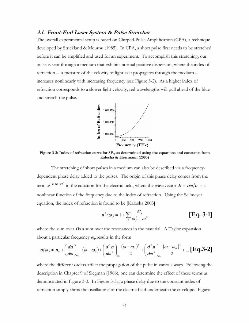
31
3.1. Front-End Laser System & Pulse Stretcher The overall experimental setup is based on Chirped-Pulse Amplification (CPA), a technique
developed by Strickland & Mourou (1985). In CPA, a short pulse first needs to be stretched
before it can be amplified and used for an experiment. To accomplish this stretching, our
pulse is sent through a medium that exhibits normal positive dispersion, where the index of
refraction – a measure of the velocity of light as it propagates through the medium –
increases nonlinearly with increasing frequency (see Figure 3-2). As a higher index of
refraction corresponds to a slower light velocity, red wavelengths will pull ahead of the blue
and stretch the pulse.
Figure 3-2: Index of refraction curve for SF6, as determined using the equations and constants from Kalosha & Herrmann (2003)
The stretching of short pulses in a medium can also be described via a frequency-
dependent phase delay added to the pulses. The origin of this phase delay comes from the
term ( )tkzie ω−− in the equation for the electric field, where the wavevector cnk ω= is a
nonlinear function of the frequency due to the index of refraction. Using the Sellmeyer
equation, the index of refraction is found to be [Kalosha 2003]
∑ −+=
i i
iCn22
2 1ωω
ω )( [Eq. 3-1]
where the sum over i is a sum over the resonances in the material. A Taylor expansion
about a particular frequency ω0 results in the form
( ) ( ) ( )...)( +
−
+
−
+−⋅
+≈
22
3
0
3
32
0
2
2
00
000
ωωω
ωωω
ωωω
ωωωω d
nd
d
nd
d
dnnn [Eq.3-2]
where the different orders affect the propagation of the pulse in various ways. Following the
description in Chapter 9 of Siegman (1986), one can determine the effect of these terms as
demonstrated in Figure 3-3. In Figure 3-3a, a phase delay due to the constant index of
refraction simply shifts the oscillations of the electric field underneath the envelope. Figure

32
3-3b demonstrates the effect of a linearly increasing index of refraction, which is often
termed group delay as it is the entire envelope that is shifted instead of just the phase.
Figure 3-3c shows a stretching of the pulse due to the second-order dispersion, which
describes the dispersion of the group delay, or equivalently how the group velocity changes
with respect to wavelength. The asymmetric pulse-splitting due to third-order dispersion is
shown in Figure 3-3d. Ideally, the normal positive dispersion experienced by the pulse in the
stretcher should be exactly matched by the negative dispersion in the compressor, which will
be discussed again in §3.4.
Figure 3-3: Effect of various orders of the dispersion on a short pulse: (a) a constant phase shift simply adjusts the phase of the oscillation – depicted is a phase shift of ; (b) first-order dispersion results in a delay of the pulse in time; (c) second-order dispersion stretches the pulse; (d) third-order dispersion
stretches and splits the pulse
The mode-locked oscillator used to provide the short pulses is a commercial
Femtolasers Scientific Pro that generates 10fs pulses with a central wavelength of 800nm.
These are produced at a rate of ~75MHz and an average power of 400mW. A quarter of
this power is split off and then, to prevent self-phase modulation later in the system, is
stretched by propagation through a 5cm glass block and a 5cm water cell, where the two
media are used simply because of their availability in the lab. No phase distortions from self-
phase modulation occur during this stretching, as the pulses only contain ~1nJ of energy and
have a beam diameter of ~2mm FWHM. These pulses are then focussed into a ~100m
polarization-maintaining (PM) fibre, which provides the dual purpose of further stretching
the pulses using the normal positive dispersion of the fibre (to ~1ns), and transporting the
pulses to Dr. Strickland’s laboratory, where they are used to seed a two-colour regenerative
amplifier. A polarization-maintaining fibre was used as opposed to a simple single-mode
fibre as a frequency-dependent polarization rotation was observed in the original single-
mode fibre stretcher. This frequency-dependent polarization would generate holes in the
spectrum after sending the seed through a polarizing Faraday Isolator, hence making it
difficult to seed the two wavelengths in the regenerative amplifier well. While this problem

33
was not observed with the PM fibre, it was found by using a waveplate and polarizer that it
did not actually maintain the initial linear polarization, but instead randomized it across the
entire spectrum. This was certainly not expected, but is still preferable to the frequency-
dependent behaviour exhibited by the single mode fibre, and did allow for sufficient seeding
of the regenerative amplifier. An example of the spectrum obtained from the oscillator is
given in Figure 3-4.
Figure 3-4: Measured spectrum of the Femtolasers Scientific Pro oscillator
3.2. Dual-Wavelength Regenerative Amplifier
Figure 3-5: Illustration of the dual-wavelength regenerative amplifier
The main advantage of this laser system for the study of transient MRG is the ability to
provide two high-energy broadband pulses shifted from each other in frequency. Key to the
dual-wavelength operation of this system is the lab-built regenerative amplifier (Regen)
reported in Zhang et al (2000), where it is seeded by the ultra-broad bandwidth of the
oscillator pulses as opposed to the original lab-built two-colour oscillator. As the
maintenance and operation of this system was critical to this study, its design and alignment
are presented in appendices A and B respectively.

34
In brief, a single ultra-broad bandwidth pulse from the oscillator is injected into a
four-mirror cavity using a combination of a polarizer and a polarization-switching element
called a Pockels Cell. It is then focussed into a Titanium-doped Sapphire crystal
(Ti:Sapphire), which is optically excited using a frequency-doubled Spectra-Physics Nd:YAG
laser (Neodymium-doped Yttrium-Aluminium-Garnet laser). A system of prisms act to
disperse the infrared pulse in the cavity, splitting it into two pulses of separate frequencies
defined by slits in the cavity. Once the pulses have attained their maximum energy, as
determined by a diode collecting the light leaked through one of the mirrors, they are ejected
again via the polarizer/Pockels Cell combination.
3.2.1. Seeding of the Amplifier
A schematic of the seeding apparatus is shown in Figure 3-6. After entering the laboratory
through the PM fibre, the oscillator pulses are sent through a Faraday Isolator (FI) to
prevent damage to the fibre optic by the returning beams. That is, any light that is sent back
along the path of the seed will be redirected. This is accomplished by using a pair of
polarizers in conjunction with a Faraday rotator, an element that applies a magnetically-
induced direction-dependent rotation to the polarization of the beam via the Faraday effect
[Hecht 2002]. This element also includes a half-wave plate to optimize its isolating action
for a particular wavelength, which is tuneable in the two-colour regenerative amplifier.
Figure 3-6: Two-colour seeding of the Regen
As mentioned earlier, the polarization of the seed beam is randomized by the PM
fibre, and as such it is split by the first polarizer of the Faraday Isolator. The rejected
polarization is sent to a fast diode (D) to act as a clock signal for the Pockels Cell and
detection instruments. The transmitted seed is spectrally separated using a system of three
prisms, as there is then independent control of the seeding for the two wavelengths in the
Regen. By aiming the back mirrors slightly downwards to a lowered mirror, the pulses are

35
recombined and sent through a broadband half-wave plate ( 2λ ) before going through a
second Faraday Isolator. Two Faraday Isolators are used because it was observed that a
single FI could not fully prevent the two pulses generated in the Regen from damaging the
fibre optic, given their large separation in frequency. Note that the convoluted path of the
beam before the second Faraday Isolator is designed to allow the returning pulses from the
Regen to go straight through, reducing the potential for spatial chirp and misalignment of
the beams. A significant divergence between the two amplified pulses was observed when
the Faraday Isolator was used in the opposite manner (sending the seed straight through and
making the Regen pulses reflect at an angle), as the reflection through the polarizer is not
actually at a 90o angle, making it act as a wedge. This wedge-like behaviour was also the
reason the independent control of the two seed pulses was required and installed once the
Faraday Isolator was turned around.
To control how the seed pulses enter and exit the cavity, a combination of a
polarizer and a polarization switch is used in the cavity. The polarization switch is a
commercial Medox Pockels Cell, which uses a voltage-dependent birefringence called the
Pockels effect to adjust the polarization of the beam as it passes through. During regular
operation, the birefringence is set to make the cell act as a quarter-wave plate with the
voltage off, and with the two consecutive pulses of different voltages, it is set to act first as a
half-wave plate, and then as a three-quarters-wave plate. Its operation is as follows:
1. An initially s-polarized seed pulse (polarized perpendicular to the optical bench),
reflects off the polarizer
2. With the voltage off, the seed becomes circularly polarized light as it first goes
through the Pockels Cell. It is immediately reflected by a plane mirror back through
cell again, changing it to p-polarized light (parallel to the optical bench)
3. Before the next seed pulse can enter the cavity, a voltage pulse is sent to the
Pockels Cell to convert it to a half-wave plate. Therefore, any subsequent seed
pulses will simply be reflected out of the cavity by the polarizer, as they will be
rotated and then counter-rotated upon traversing the cell, returning to s-polarization
4. The trapped p-polarized seed pulse oscillates back and forth in the cavity, as the
Pockels Cell again only rotates and counter-rotates the polarization.
5. After the seed pulse has been amplified, the second voltage pulse puts the
Pockels Cell into its three-quarter-wave mode, ejecting the seed from the cavity as it

36
becomes s-polarized again. The Pockels Cell is then electrically grounded in
preparation for the next pump pulse.
3.2.2. Amplification
The amplifier itself is essentially a two-colour laser, and can generate its own pulses through
the amplification of its own spontaneous emission. To differentiate this light from that of
the amplified seed pulse, the amplified spontaneous emission of the Regen is referred to
simply as the ASE as opposed to the amplified seed pulse. This ASE will have the same
frequency spectrum as the seed would have during amplification in the Regen, however it
lacks the definite phase relationship that is characteristic of a mode-locked pulse, and is
therefore not compressible. Any ASE that is generated along with the seed pulse will
therefore act as a background and compete for the gain in the amplifier, and as such it is
desirable to align the seed beam into the Regen as well as possible to maximize its gain and
minimize the ASE. In particular, there must be more seed light coupled properly into the
cavity than there would be ASE at the time of the seed injection. To aid in this effort, the
seed is spectrally separated prior to the Regen assembly allowing for total and independent
control of the two colours. A fast diode is also placed behind a mirror in the Regen to
monitor the small amount of light that leaks through, allowing one to observe the radiation
in the cavity as a function of time to aid in the alignment (see the element labelled D in
Figure 3-5). A characteristic trace from this diode is illustrated in Figure 3-7, where the
sharp peaks are due to the seed pulse and the broad background is from the ASE. The time
between the peaks corresponds to the round-trip time of the pulse in the cavity. By
monitoring the ratio of the seed signal to that of the ASE, one can optimize the seed
alignment. The point at which the seed is injected with the same power as the existing ASE
is when VSeed/VASE is 2:1, such that the seed peaks sitting on the background are as intense
as the background itself. A typical value for this ratio obtained in our experiments is 40:1.
Figure 3-7: Characteristic trace of the fast diode from behind the curved mirror in the Regen. (a) Pockels Cell switches the beam out when the energy of the pulse is at a maximum. (b) Pockels Cell switches the beam out after it has diminished due to losses in the cavity.

37
Notice the interplay between the gain and loss in the cavity in Figure 3-7b. As the
light oscillates in the cavity, it successively takes more and more energy stored in the
Ti:Sapphire crystal. This continues until the energy gained from the crystal is less than the
energy lost due to imperfections in the cavity, such as the small transmission through the
cavity mirrors monitored by the diode. At this point the energy in the pulse decreases with
each pass such as depicted in Figure 3-7b, but not necessarily in the symmetric fashion as
illustrated. To obtain the highest pulse energies, the Pockels Cell is switched from its half-
wave voltage (where it acts as a half-wave plate), to its three-quarter-wave voltage (which
ejects the pulses from the Regen), when the diode signal reaches its peak, as shown in Figure
3-7a. This technique of selecting when to eject the pulses is called cavity dumping.
One problem that has not been completely remedied is the generation of pre-pulses
in the beam. Each time the seed pulse oscillates in the Regen cavity, as small amount of light
is switched out by the polarizer due to the small imperfections in the cavity. This leakage
can be measured by putting a diode into the laser beam such as in Figure 3-8 (along with
some very strong attenuation, such as multiple pieces of paper). Because of this, the energies
measured during the experiments are not contained in a single pulse, but spread over a
number of them. In Figure 3-8 about 60% of the energy is contained in the main pulse.
This unfortunately was not considered until after the experiments had been completed, and
so there is no complete record of the pre-pulses for each scan. However, Figure 3-8 was a
pretty standard trace, and as such it will be assumed that approximately 60% of the recorded
energy is contained in the main laser pulse for the entire study.
Figure 3-8: Signal from a diode placed directly in the beam

38
3.2.3. Beam Control
It is important in the operation of the dual-wavelength Regen that one can independently
manipulate the characteristics of the two beams, such as their central wavelengths, their
bandwidths, and the relative energy and timing between them. As such, the cavity was
designed to include elements that could provide this control. The wavelength and
bandwidth of the individual beams can be adjusted using slits that are placed after the
prisms, as the spectra are then spatially dispersed. The slit width allows one to reduce the
bandwidth of the pulses, and the slit positions control the central wavelengths. The relative
timing between the pulses can be adjusted by using a translation stage on one of the back
mirrors (see Figure 3-5), where it is desirable for the two pulses to be overlapped in time.
To adjust the energy of the pulses, one can insert a polarizer/half-wave plate combination in
one of the arms to provide a variable attenuator. This is placed in the short-wavelength arm
of the Regen, as the shorter wavelengths tend to experience more gain than longer ones, and
can therefore afford the loss. In a limited way, one can also adjust the energy balance by
adjusting the position of the pump beam in the crystal using its lens. This controls the
relative gain seen by each beam, as the two beams diverge slightly in the crystal due to the
dispersion of the index of refraction, as shown in Figure 3-9. The typical energy in the
pulses from the Regen was about 2.5mJ for pulses with central wavelengths of 780nm and
830nm, which is consistent with what was obtained in Zhang et al (2000).
Figure 3-9: Illustration of the divergence of the two pulses as they propagate through the crystal. The short-wavelength beam is denoted Sλ, and the long-wavelength beam is denoted Lλ.
3.3. Multipass Amplifier To increase the energy of the pulses further, the high-energy multipass amplifier developed
by Xia et al (2002) was used. As opposed to a regenerative amplifier there is no cavity; it is
instead through the redirection of the beam by a series of mirrors that the pulses go through
the crystal multiple times (Figure 3-10). The somewhat complicated setup of using two
turning mirrors on each pass was used due to the observation in Xia et al (2002) that the two
colours of the Regen were spatially separated by 1mm, and that by using the two turning-
mirror setup, the beam separation could be reduced with each successive pass. Going into

39
the crystal from the right, the short-wavelength beam would be below the long-wavelength
beam as depicted in Figure 3-9 and as such should come together as they pass through the
crystal, but to do this from the left, the short-wavelength beam should be on top. Switching
the relative position of the beams is not possible with a single redirecting mirror, and so a
pair of them are used.
Figure 3-10: Illustration of the multipass amplifier when working in a three-pass operation. This was increased to five passes for much of the experiment to increase the available energy.
While the losses for each pass were consistent with the small reflection losses
expected (~6% loss with each pass), the net gain in the system was poor compared to that
reported in Xia et al (2002). The total energy in the pulses was 14mJ directly out of a five-
pass amplifier, which is approximately a five-fold increase from the typical 2.5mJ out of the
Regen. This is compared to the 30mJ output that was reported in Xia et al (2002) with input
pulses of 1.5mJ. The discrepancy between these amplification factors could in retrospect be
due to the new seeding arrangement. The multipass design shown in Figure 3-10 was used
to compensate for a separation of the beams, which was thought to have been caused by the
divergence of the beams through the Ti:Sapphire crystal in the Regen. However, recall the
discussion in §3.2.1 about the Faraday Isolator acting as a wedge, due to the fact that the
reflection through it’s polarizer was not exactly 90o. In the configuration of Xia et al (2002),
the Faraday Isolator was set in such a way that the Regen pulses would go through this
wedge, and thus would diverge given their separation in frequency. By switching this
configuration to instead make the seed go through this wedge, the divergence of the Regen
pulses was corrected before the multipass, and therefore instead of bringing the two pulses
together, the two turning-mirror setup would actually be separating them. This was realized
after our experiments, however at the time it was decided that 14mJ was enough to conduct
our investigations.
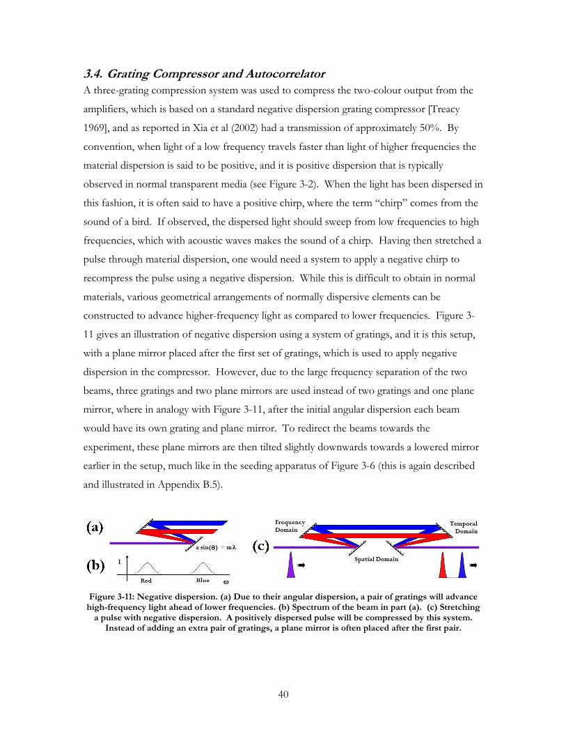
40
3.4. Grating Compressor and Autocorrelator A three-grating compression system was used to compress the two-colour output from the
amplifiers, which is based on a standard negative dispersion grating compressor [Treacy
1969], and as reported in Xia et al (2002) had a transmission of approximately 50%. By
convention, when light of a low frequency travels faster than light of higher frequencies the
material dispersion is said to be positive, and it is positive dispersion that is typically
observed in normal transparent media (see Figure 3-2). When the light has been dispersed in
this fashion, it is often said to have a positive chirp, where the term “chirp” comes from the
sound of a bird. If observed, the dispersed light should sweep from low frequencies to high
frequencies, which with acoustic waves makes the sound of a chirp. Having then stretched a
pulse through material dispersion, one would need a system to apply a negative chirp to
recompress the pulse using a negative dispersion. While this is difficult to obtain in normal
materials, various geometrical arrangements of normally dispersive elements can be
constructed to advance higher-frequency light as compared to lower frequencies. Figure 3-
11 gives an illustration of negative dispersion using a system of gratings, and it is this setup,
with a plane mirror placed after the first set of gratings, which is used to apply negative
dispersion in the compressor. However, due to the large frequency separation of the two
beams, three gratings and two plane mirrors are used instead of two gratings and one plane
mirror, where in analogy with Figure 3-11, after the initial angular dispersion each beam
would have its own grating and plane mirror. To redirect the beams towards the
experiment, these plane mirrors are then tilted slightly downwards towards a lowered mirror
earlier in the setup, much like in the seeding apparatus of Figure 3-6 (this is again described
and illustrated in Appendix B.5).
Figure 3-11: Negative dispersion. (a) Due to their angular dispersion, a pair of gratings will advance high-frequency light ahead of lower frequencies. (b) Spectrum of the beam in part (a). (c) Stretching a pulse with negative dispersion. A positively dispersed pulse will be compressed by this system. Instead of adding an extra pair of gratings, a plane mirror is often placed after the first pair.

41
To determine the dispersion necessary to compress the pulses, the pulse widths are
monitored by a non-collinear single shot autocorrelator [Janszky 1977], where a schematic of
this device is shown in Figure 3-12. Essentially, one of the two beams is sent through a
periscope to switch the polarization from p-polarized (parallel to the optical bench), to s-
polarized (perpendicular to the optical bench). The light is then split using a 50-50
beamsplitter, where one arm contains a delay line to time up the pulses. The two beams are
then sent at an angle through a birefringent frequency-doubling crystal, which in this case is
a 0.25mm thick Barium Borate (BBO) crystal. The overlap of the beams in the crystal
produce frequency-doubled light, where the direction of the resulting beam is given by the
sum of the wavevectors from the two pulses, and its width gives a measure of the temporal
duration of the pulses via the pulse autocorrelation. The 2ω light is then recorded on a CCD
camera to give a single-shot determination of the pulse length.
Figure 3-12: Single-shot non-collinear autocorrelator.
To get a sense of how this gives a measure of the temporal duration, refer to Figure
3-13. As the two pulses propagate through the crystal (propagation is shown by the dotted
lines), they generated frequency-doubled light in three directions: each individually makes a
frequency-doubled beam along its own path, and when they overlap they produce frequency-
doubled light that, due to momentum conservation, propagates in a direction that is the
vector sum of the directions of the two pulses. The integrated sum-frequency light that is
generated from this overlap is called their autocorrelation, and in general the shape of the
distribution depends on both the temporal and spatial profile of the pulses. The resulting
distribution recorded by a camera gives a measure of the pulse duration (see Figure 3-14),
where the width of the autocorrelation distribution must be scaled by an appropriate form
factor when determining the pulse width, to take into account the fact that the pulses
overlap more in the centre of the distribution than at the edges. A simple approximation of
the autocorrelation width is given by Kolmeder et al (1979), where it is linear with respect to

42
the pulse length if the longitudinal width of the pulse (c times the pulse duration), is less than
one third of the beam diameter. As the beams used in this experiment were 3mm FWHM,
the maximum pulse duration that can be measured should be approximately 3ps.
Figure 3-13: Sum-frequency generation using two identical non-collinear pulses. Note how the vertical dimensions of the generated light depend on the temporal width of the pulses.
Figure 3-14: Sample Autocorrelation. (a) Time-integrated sum-frequency signal as recorded by the
camera. (b) Profile as determined by the camera (summed along the y-axis)
To characterize the operation of the autocorrelator, two scans needed to be
conducted. The first was a calibration of the time per pixel as recorded on the CCD camera,
where one pulse was delayed with respect to the other and the centre of the generated
distribution was recorded. The result of the calibration is plotted in Figure 3-15a, where a
linear regression found a scaling factor of about 7.3fs per pixel. Note that the time scale in
Figure 3-15a has been divided by 2 , which corresponds to the autocorrelation form factor
for Gaussian pulses. This form factor was included in the calibration to simply save time in
the analysis, as it was assumed for the duration of this experiment that the pulses were
Gaussian.

43
Figure 3-15: Scans using the autocorrelator. (a) Mapping the pulse delay to the peak position on the CCD camera. (b) Mapping the grating position to pulse width. The black line shows the width of the
long-wavelength pulse, and the grey line shows the width of the short-wavelength pulse.
The second scan was a study of the pulse width with the grating position, which used
the previous calibration to determine the pulse widths as observed by the CCD camera.
This is shown in Figure 3-15b, where it was found that the maximum measurable pulse
width was approximately 1.4 picoseconds, which is not too far from the predicted maximum
pulse width of 3ps. The grating position is not taken with respect to anything meaningful –
it is simply measured from a convenient spot on the optical bench. However, one thing to
note is that the long wavelength grating is found closer to the first grating than the short
wavelength grating. This is opposite to what would be expected, as can be seen in Figure 3-
11 where the red beam (long wavelength) is further away from the first grating than the blue
beam (short wavelength). This discrepancy can be attributed to a mismatch in the third
order dispersion experienced during the stretching and compression of the pulses. As a
significant amount of second-order dispersion was required to stretch the pulses, a large
amount of third-order dispersion was added as well, which could not be perfectly matched
by the gratings [Backus 1998]. This mismatch limits the compression possible with this
setup, and while it was not corrected for this experiment there are plans to replace the long
fibre used to stretch the seed with a grating stretcher, which in principle should be better
matched to the grating compressor.
3.5. Hollow Fibre Assembly As is often used for nonlinear optics in a gas, this experiment was conducted in a fused-silica
hollow dielectric waveguide, primarily to increase the length of the beam focus (which in this
case was increased from approximately 4cm to 1m), but also to contain the beam in a single,

44
highly selective mode. This is especially important in MRG because of the detrimental
effects of the Raman defocusing described in Syed et al (2000) and Losev et al (2002a).
Described originally by Marcatili & Schmeltzer (1964) using a modal analysis, the
waveguiding properties may at first seem counter-intuitive, given that the light is trapped in a
region with a low index of refraction as opposed to a regular fibre-optic waveguide where a
beam is trapped in a region with a high index of refraction. However, the conditions
necessary for coupling efficiently into the fibre [Abrams 1972; Mohebbi 2004], mean that the
beams are actually focussed at relatively small angles into the fibre, roughly at 0.2o. Upon
consideration of the Fresnel coefficients of a dielectric, the waveguiding nature of the hollow
fibre can be realized as simply small-angle reflections from the inner surface [Nisoli 1996],
given that any smooth surface acts as a mirror at small angles.
Two hollow fibres were used in the experiment, one with an inner diameter of
250µm and one with an inner diameter of 129µm. Two different fibres were used to
examine the effect of their plasma-like dispersion – according to the modal analysis of
Marcatili & Schmeltzer (1964) the hollow fibre exhibits negative dispersion, where longer
wavelengths travel slower than shorter ones. Balanced with the normal dispersion of SF6,
this should produce zero dispersion point at a particular frequency. This is illustrated in
Figure 3-16, where the group delay is plotted for (a) SF6 by itself, (b) SF6 in a hollow fibre
with an inner diameter of 250µm, and (c) SF6 in a hollow fibre with an inner diameter of
129µm. The group delay gives a measure of how much one frequency is delayed with
respect to the other, where the minimum corresponds to the point of zero dispersion. Note
that these group delays are all taken relative to the group delay of SF6 at zero frequency, and
all are calculated assuming the SF6 is at a pressure of 1atm.
Figure 3-16: Balance between the normal dispersion of SF6 and the negative dispersion of the hollow fibre. (a) Group delay (GD), of SF6 relative to the zero-frequency GD at a pressure of 1atm. (b) GD of
SF6 in a 250µµµµm hollow fibre at 1atm. (c) GD of SF6 in a 129µµµµm hollow fibre at 1atm.

45
An example of the setup of one of the fibres is illustrated in Figure 3-17. To couple
best into the fibres, the 1/e2 beam size at the entrance (or 1/e diameter of the field), should
be approximately 60% of the inner diameter of the fibre. As such, we used lenses of 750mm
and 300mm to focus into the two fibres. A variable attenuator was placed in front of the
apparatus to control the energy, and after the chamber the beam was collimated and
redirected towards a variety of diagnostics.
Figure 3-17: Illustration of the hollow fibre apparatus. Note the inset showing small-angle reflections.
The high-pressure fibreglass chamber designed by Mr. Robin Helsten contained a v-
groove aluminium bar to seat the hollow fibre, which was made as straight as possible to
minimize transmission losses. To facilitate alignment, two X-Y translation mounts were
positioned at the tips of the fibre, which should provide independent control of the position
of the entrance of the fibre and the angle of the fibre. The ends of the fibre were sealed
with 2mm thick windows plus end caps, with a vacuum-grade seal provided by greased O-
rings and a gas delivery system designed and built by Mr. Jean-Paul Brichta. This chamber
was filled with SF6 gas with pressures from one to three atmospheres. Typically,
transmission through the assembly with the 250µm fibre was about 17%, and that through
the 129µm fibre was about 7%. This is low compared to what is expected [Marcatili 1964],
which we attribute to coupling and surface-roughness in the fibres.
The alignment of a hollow fibre was non-trivial to determine initially. Indeed, it is
nearly impossible to align the beams through the fibre using mirrors before the apparatus,
and as well it is nearly impossible to determine the best alignment using a simple power
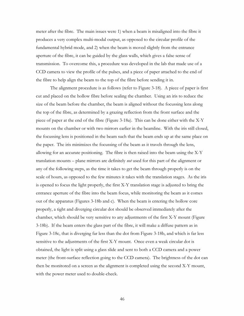
46
meter after the fibre. The main issues were 1) when a beam is misaligned into the fibre it
produces a very complex multi-modal output, as opposed to the circular profile of the
fundamental hybrid mode, and 2) when the beam is moved slightly from the entrance
aperture of the fibre, it can be guided by the glass walls, which gives a false sense of
transmission. To overcome this, a procedure was developed in the lab that made use of a
CCD camera to view the profile of the pulses, and a piece of paper attached to the end of
the fibre to help align the beam to the top of the fibre before sending it in.
The alignment procedure is as follows (refer to Figure 3-18). A piece of paper is first
cut and placed on the hollow fibre before sealing the chamber. Using an iris to reduce the
size of the beam before the chamber, the beam is aligned without the focussing lens along
the top of the fibre, as determined by a grazing reflection from the front surface and the
piece of paper at the end of the fibre (Figure 3-18a). This can be done either with the X-Y
mounts on the chamber or with two mirrors earlier in the beamline. With the iris still closed,
the focussing lens is positioned in the beam such that the beam ends up at the same place on
the paper. The iris minimizes the focussing of the beam as it travels through the lens,
allowing for an accurate positioning. The fibre is then raised into the beam using the X-Y
translation mounts – plane mirrors are definitely not used for this part of the alignment or
any of the following steps, as the time it takes to get the beam through properly is on the
scale of hours, as opposed to the few minutes it takes with the translation stages. As the iris
is opened to focus the light properly, the first X-Y translation stage is adjusted to bring the
entrance aperture of the fibre into the beam focus, while monitoring the beam as it comes
out of the apparatus (Figures 3-18b and c). When the beam is entering the hollow core
properly, a tight and diverging circular dot should be observed immediately after the
chamber, which should be very sensitive to any adjustments of the first X-Y mount (Figure
3-18b). If the beam enters the glass part of the fibre, it will make a diffuse pattern as in
Figure 3-18c, that is diverging far less than the dot from Figure 3-18b, and which is far less
sensitive to the adjustments of the first X-Y mount. Once even a weak circular dot is
obtained, the light is split using a glass slide and sent to both a CCD camera and a power
meter (the front-surface reflection going to the CCD camera). The brightness of the dot can
then be monitored on a screen as the alignment is completed using the second X-Y mount,
with the power meter used to double-check.
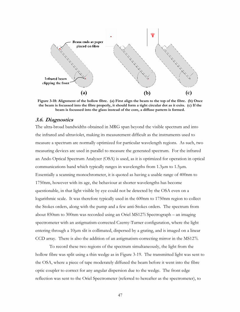
47
Figure 3-18: Alignment of the hollow fibre. (a) First align the beam to the top of the fibre. (b) Once the beam is focussed into the fibre properly, it should form a tight circular dot as it exits. (c) If the
beam is focussed into the glass instead of the core, a diffuse pattern is formed.
3.6. Diagnostics The ultra-broad bandwidths obtained in MRG span beyond the visible spectrum and into
the infrared and ultraviolet, making its measurement difficult as the instruments used to
measure a spectrum are normally optimized for particular wavelength regions. As such, two
measuring devices are used in parallel to measure the generated spectrum. For the infrared
an Ando Optical Spectrum Analyzer (OSA) is used, as it is optimized for operation in optical
communications band which typically ranges in wavelengths from 1.3µm to 1.5µm.
Essentially a scanning monochrometer, it is quoted as having a usable range of 400nm to
1750nm, however with its age, the behaviour at shorter wavelengths has become
questionable, in that light visible by eye could not be detected by the OSA even on a
logarithmic scale. It was therefore typically used in the 600nm to 1750nm region to collect
the Stokes orders, along with the pump and a few anti-Stokes orders. The spectrum from
about 850nm to 300nm was recorded using an Oriel MS127i Spectrograph – an imaging
spectrometer with an astigmatism-corrected Czerny-Turner configuration, where the light
entering through a 10µm slit is collimated, dispersed by a grating, and is imaged on a linear
CCD array. There is also the addition of an astigmatism-correcting mirror in the MS127i.
To record these two regions of the spectrum simultaneously, the light from the
hollow fibre was split using a thin wedge as in Figure 3-19. The transmitted light was sent to
the OSA, where a piece of tape moderately diffused the beam before it went into the fibre
optic coupler to correct for any angular dispersion due to the wedge. The front edge
reflection was sent to the Oriel Spectrometer (referred to hereafter as the spectrometer), to

48
avoid absorption in the ultraviolet portions of the spectrum by transmission through the
wedge. It was then attenuated by a second reflection from a wedge to avoid saturation in the
spectrometer, where only the front-surface reflection from each wedge was used. This
reflective attenuation was chosen as opposed to using the absorptive neutral density filters
available in the lab, because even though their response should be flat across the spectrum, it
was found that these filters attenuated longer wavelengths more than the short-wavelength
anti-Stokes orders. This could possibly have been due to some nonlinear absorption or
saturation effect, as the strong pump beams are in the infrared and should reach the filters
before the anti-Stokes orders due to dispersion.
Figure 3-19: Schematic of the measurement apparatus. The light transmitted through the second wedge was blocked.
In terms of collecting the data, the OSA would output a simple text file with two
columns of data, one for the wavelength and one for the intensity. As the dynamic range
was very good, only one scan needed to be taken for a given spectrum. While the
spectrometer would also output two columns of data, it suffered from a number of issues
that made the analysis problematic. A typical output was shown in Figure 3-20, where the
Pixel number on the linear CCD runs from 0 to 2009, and the intensity reading runs from 0
to 4095. The main problems with using the spectrometer were 1) it could not be triggered,
with the result that laser shots were occasionally missed or extra ones added, increasing the
range of intensities over which saturation was observed, and 2) there was a very large
threshold in its intensity measurement, which reduced the usable dynamic range to at best a
single order of magnitude. This small dynamic range necessitated the accumulation of a
number of scans for each spectrum, where from one scan to the next the integration time of
the CCD camera was increased by a factor of 2. To ensure that the scans were directly
comparable, for each integration time the number of shots to average was chosen to keep
the number of total number of shots constant. A linear regression between the two scans
was then determined in Excel to patch the scans together and form a single spectrum, which
resulted in a dynamic range larger than that possible with a single scan.

49
Figure 3-20: Typical plot from the Oriel Spectrometer
To demonstrate how these behaviours affect the analysis, refer to the plots in Figure
3-21. The intensity of two successive scans were plotted against each other (and therefore
two successive integration times), where each data point is at a coordinate of
)(),( nIntegratio Long of Intensity n,Integratio Short of Intensityyx =
for a particular pixel number. One would predict a linear regression of y = 2x, as the
integration time had simply increased by a factor of two. However, as can be seen in Figure
3-21a, this plot is far from linear, which is due to saturation effects and the fact that the
spectrometer could not be triggered, which contributes to the curvature of the plot at lower
intensities. Therefore, any data points that did not exhibit a linear behaviour were deleted.
Specifically, the data points at the threshold of the detector are deleted (where the intensity
of the short integration time is less that 100), as in (Figure 3-21b), and any near the
saturation of the detector are deleted (where the intensity of the long integration time is
greater than 3000) (Figure 3-21c). To avoid skewing the fit, all points along the x-axis after
the first saturated data point are deleted as well (see the shaded areas in Figure 3-21). A
least-squares linear fit is then determined with the remaining points.
Figure 3-21: Generating a linear regression with the spectrometer. (a) Raw data, where the intensities between successive scans are plotted against each other. (b) Any points with an x-value below 100 are deleted. (c) Starting at the first point with a y-value above 3000, all points with higher x or y values are
deleted. The resulting linear regression is shown.

50
Note that in Figure 3-21c, the resulting linear regression gives an intercept of 377,
which implies that there is a threshold intensity necessary before the CCD reads an intensity.
On average, this intercept was about 720, which means that out of the total possible signal
that can be read (4095 + 720), 15% of the signal was below the threshold of the detector.
Of the usable signal (3000 + 720), 20% is below the threshold, resulting in a dynamic range
that is less than an order of magnitude. To overcome this poor range, a series of at least 6
scans were compiled to generate a single spectrum. Starting with the most sensitive scan
(the one with the highest integration time), each successive scan was scaled by what was
obtained in the linear regression, which when plotted would look like Figure 3-22a. To clean
up the spectrum, all intensities below 100 or above 3000 for each scan was deleted, resulting
in final spectrum much like Figure 3-22b. Note that occasionally a number of floating peaks
can be observed in different parts of the spectrum as shown in the circled area of Figure 3-
22b. This is predominantly due to intensity fluctuations in the laser beam, as MRG is a
highly nonlinear process and a single compiled spectrum takes approximately 15 minutes to
complete. As such, these floating peaks give a sense of the errors bars in the spectra.
Figure 3-22: Compiled spectrum. (a) Each spectrum is scaled by the constants determined in the linear regression. (b) The spectra are cleaned up by ignoring data points with intensities below 100 or
above 3000, on a scale of 0 to 4095. Note the residual multi-peak structure due to intensity fluctuations.

51
4. Experimental Results & Discussion The primary aim of this study was to determine the potential of Dr. Strickland’s two-colour
laser system for the production of high-energy few-femtosecond pulses, by utilizing
multifrequency Raman generation in the transient regime. To this end, we first had to
establish a reproducible and reliable experimental procedure, during which we fine-tuned or
rebuilt each part of the system to maximize the generated bandwidth. After a proof-of-
principle measurement where at least 30 Raman orders were generated, attention turned to
the scaling of the bandwidth as the energy in the pump beams was adjusted. The results
obtained from this scan indicated a number of promising features, such as the preferential
growth of the high-frequency anti-Stokes orders and the formation of a plateau on the scale
of the short-wavelength pump beam. The scan also demonstrated the limiting effect self-
phase modulation has on the potential bandwidth, which provided insight into how to
further optimize our apparatus.
Our most recent investigations involved the effect of dispersion of the generated
spectrum. As mentioned in §3.5 the size of a hollow fibre affects its dispersion
characteristics, and so a number of studies were conducted in a smaller-diameter fibre where
these effects should be apparent. It was shown that dispersion was a very important
determinant in the behaviour of the Raman generation, as a very dramatic and counter-
intuitive enhancement was observed as the pressure was decreased from 3atm to 1atm.
Furthermore, the structure of the generated Raman orders at lower pressures was very
interesting, and may possibly point to the interesting physics of soliton formation, though
not necessarily the few-femtosecond multifrequency solitons discussed in Kaplan (1994).
4.1. Procedure and Measurement As in any new experimental investigation, this study experienced a period of trial and error
when developing and fine-tuning the experimental procedure. As such, out of the nearly
1000 spectra taken, only a relatively small subset are actually meaningful. Many of the issues
encountered were to do with the measurement of the incredibly large bandwidths, most of
which were discovered only upon analysis of the data.
Originally the OSA was used to observe the entire generated spectrum, as its quoted
range of 1750nm to 400nm should have allowed for the collection of a large number of
Stokes and anti-Stokes orders. During these initial measurements with the OSA, at least

52
three factors were working to corrupt the data, as will be described with the help of Figure
4-1. First and foremost, while the scale of the OSA was in nanowatts on a potential scale of
milliwatts, a number of the peaks were strongly saturating the detector (the seven central
peaks in Figure 4-1). This saturation was confirmed when absorptive filters were placed in
the beam with little effect on the level of the peaks. With some thought this is not surprising
– the scale describes the average power of the beam, but the pump pulses being used had
peak powers on the order of 100MW. With sufficient attenuation, the intensities as recorded
by the OSA eventually demonstrated a linear behaviour.
Figure 4-1: Early Ando spectrum and reflectivity curve of a mirror used after the hollow fibre, © Newport Corporation – Used by permission from
http://www.newport.com/store/genproduct.aspx?id=141092&lang=1033&Section=Spec.
Secondly, the mirrors that were being used after the fibre had reflectivity curves that
did not cover the entire generated spectrum, in particular the silver BD.1 and ER.2 coated
mirrors from Newport. The BD.1 curve taken from the Newport website is shown in
Figure 4-1, and the corresponding reflectivity range is shown within the arrows. Note that
below the pump frequencies of 352THz and 375THz the intensity of the spectra drop
dramatically, which would be expected as the reflectivity drops below 428THz. The final
problem encountered is highlighted by the arrow pointing down at the Raman order at
~500THz. This order, which is very weak as depicted by the OSA, was easily visible to the
naked eye. Given this fact along with 1) the other orders were strongly saturated and 2) the
fact that the mirrors were nearly perfect at the wavelength of that Raman order, it was
concluded that the OSA could not properly detect wavelengths around and shorter than
600nm (500THz). As the behaviour of the OSA in this wavelength region could not to be
trusted, the spectrometer was chosen as the primary measurement device, whereas the OSA

53
was used to only monitor the Stokes orders that the spectrometer could not detect (the range
of the spectrometer was ~350THz to 1000THz).
The next issue encountered involved the scaling of the spectra to one another. As is
described in §3.6, the spectrometer suffered from a small dynamic range due to its large
threshold intensity, and as such required the compilation of a number of scans, where either
the intensity of the light or the integration time on the CCD was adjusted. Originally, both
of these techniques were used to scale the data, where the light was attenuated by using
absorptive Neutral Density filters (ND filters). Unfortunately, possibly due to the large
intensities involved in the experiment, the ND filters did not exhibit a flat attenuation as
expected, but imparted a frequency-dependent attenuation on the beam. This went
unnoticed for a significant amount of time, as it was only definitively demonstrated using the
most recent technique of compiling the spectra. Figure 4-2 gives an exceptional but
somewhat involved example of how the filter affected the light. As described in §3.6, the
most recent method of compiling the data consisted of determining a linear regression
between consecutive intensities, and using those scaling factors to patch various spectra
together. Figure 4-2a demonstrates an example where the integration time was decreased by
a factor of two, where its characteristic linear then saturation behaviour was described in
§3.6. In contrast with this regular behaviour, Figure 4-2b shows the effect an extra filter had
on the spectrum. Notice the erratic behaviour in the graph describing the filters – in some
places the intensity has even been increased with the addition of an extra filter (high x value,
low y value). The path that the curve follows is determined by the intensities of each pixel in
turn, from pixel #0 to pixel #2009. For example, the first two data points on the graph
would be (x1, y1) = (Intensity of Pixel #0 with 4 Filters, Intensity of Pixel #0 with 3 Filters)
and (x2, y2) = (Intensity of Pixel #1 with 4 Filters, Intensity of Pixel #1 with 3 Filters). This
helps to give a sense of how the attenuation changes as the wavelength increases.
Figure 4-2: Anomalous behaviour of an absorptive filter vs. a change in integration time. (a) Integration time had been changed by a factor of two. (b) An extra 50% filter was placed in the beam.

54
Figure 4-3 gives a more concrete demonstration of this erratic attenuation, where
two consecutive spectra are simply plotted as they were recorded from the Oriel. The two
features of note are denoted as (a) and (b). In (a), numerous orders in the spectrum with the
extra filter have actually grown, as opposed to the normal attenuation experienced beyond
Pixel #1100. In (b), the troughs between the Raman orders also give a good indication of
this wavelength dependence, as demonstrated by the curves drawn in the plot. To avoid
using these filters, the setup was modified such that the generated spectrum was attenuated
by the front-surface reflections off of two glass wedges before being sent into the
spectrometer, as depicted in Figure 3-19. With this arrangement, the pumps would not
saturate the spectrometer when set on the shortest possible integration time (which is
determined by the 10Hz repetition rate of the two-colour laser).
Figure 4-3: Two consecutive spectrometer plots where an extra filter had been added. (a) Some parts of the spectrum experienced an enhancement with the addition of a filter. (b) The troughs give a
sense of the wavelength-dependent attenuation, as the lines drawn on the graph show.
The final problem to be discovered was how sensitive the pulse compression was to
the wavelengths set in the Regen. As part of the normal experimental procedure, once a
small amount of MRG is observed, all possible parameters are adjusted to maximize the
generated anti-Stokes spectrum, including the relative timing between the pulses, the energy
balance, and the wavelength separation. However, due to the intensive nature of the
autocorrelation measurement, and the fact that it required redirecting the laser beam, the
compression was typically set before aligning the beams into the fibre. It was only recently
discovered that by adjusting the wavelengths a few nanometres (within the bandwidth of the
pulses), the pulse duration could as much as double in length. This could possibly be due to
the mismatch between the third-order dispersions of the fibre stretcher and the grating
compressor, which as mentioned is an issue that is being addressed in the laboratory by
replacing the fibre stretcher with a grating stretcher. To accommodate this sensitivity, the

55
autocorrelations are re-measured after each series of adjustments by using a removable
mirror to redirect the beam.
4.2. Demonstration of Broadband MRG The first benchmark to be met was a proof-of-principle demonstration of our capability to
produce large bandwidths. Our first attempts were conducted using the Regen alone,
however bandwidths comparable to those reported in the literature were only obtained after
the introduction of the multipass amplifier. By maximizing the compression, pressure, and
energy in the beams we were able to generate at least 30 Raman orders spanning 750THz.
In particular we used two beams centred at 384THz and 359THz with a total of 3mJ split
between them with a ratio of ~1.6: 1. Recall however the discussion in §3.2.2 where the
pre-pulses contained ~40% of the energy, and as such there was really only 1.8mJ to split
between the two beams. These beams were then compressed down to ~300fs, and were
focussed into a 250µm hollow fibre which held SF6 at a pressure of 3atm. The resulting
spectrum is shown in Figure 4-4, where the grey curve is that recorded by the OSA, and the
black is the data compiled from the spectrometer. Apparent in the graph is a large
continuum pedestal generated by the competing effect of self-phase modulation, which acts
to redirect energy from the MRG process. At this point, we had not realized the absorptive
ND filters were applying a frequency-dependent attenuation to the spectrum, and so the
most intense orders were attenuated using these filters. While the absolute scale of the
orders may therefore not be accurate, the generation of at least 30 Raman lines demonstrated
significant conversion into broadband light, especially considering that the ultraviolet orders
were visible to the naked eye (after fluorescence from white paper, much like in Figure 1-1b).
Figure 4-4: Generated MRG spectrum using two compressed pulses with a total energy of 1.8mJ.

56
As a short digression, the difference between the most recent technique described in
§3.6 and the original procedure is demonstrated in Figure 4-5, using the anti-Stokes spectra
in Figure 4-4. Note that both the shape of the spectrum and the relative scale of the peaks
are widely different between the two plots – in the second plot, the continuum base is not
apparent until the ninth anti-Stoke order, and the total scale is larger by two orders of
magnitude. This behaviour is due to the fact that in the original method, the various spectra
were scaled by matching one peak from one spectrum with the same peak from another,
assuming that the spectra were different by simply a multiplicative factor. This did not take
into account the threshold of the spectrometer, and relied on the very subjective decision of
which peaks to use from each spectrum. The method described in §3.6 is now taken as
standard, as it allows for a more accurate depiction of the spectra and because it relies on an
algorithm that does not require any subjective decision making.
Figure 4-5: Comparison between compilation methods for the spectrometer. (a) The compilation described in §3.6 (b) The original compilation. Note the different scales on the y-axis.
4.3. Demonstration of Pump-Probe MRG As both impulsive and adiabatic pump-probe schemes have been demonstrated in the
literature [Nazarkin 1999a; Liang 2000], we decided to follow suit and explore a transient
pump-probe setup. A frequency-doubled probe pulse was introduced into the system by
simply placing a BBO crystal into the pump beams as they were being focussed into the
hollow fibre. This setup generated a three-frequency probe pulse, which consisted of the
doubled frequency from each pump plus the sum-frequency between the two. As the pump
beams used in this scan were the same as those that generated the spectrum in Figure 4-4,
this led to a probe with frequencies of 718THz, 743THz, and 768THz. The results of this
experiment are shown in Figure 4-6, and are comparable to the best pump-probe results
published to date [Nazarkin 2002].

57
Figure 4-6: Modulated probe beam. The total energy contained in this spectrum was 47µµµµJ, accounting for pre-pulses.
Given the relative ease of this technique, a scan of the probe spectrum was
conducted as a function of pressure. As the gas chamber could only be used for pressures
above one atmosphere up to a maximum of 3atm, the pressures were taken at intervals of
5psi, or approximately one-third of an atmosphere. For this reason the pressure will be
quoted as being 1atm + x_psi. The resulting scan is shown in Figure 4-7, where the shaded
areas show regions of the spectrum that were saturating. Note that the BBO crystal had
been adjusted prior to the pressure scan, and as such the spectrum in Figure 4-6 is not
included in the scan. The behaviour was not found to be overly dramatic, as the main
features were 1) a bandwidth that decreased as the pressure was decreased, and 2) some
variation in the relative intensities of the peaks. These are both easily explained in reference
to §2, where the generated bandwidth was shown to depend on the pressure (i.e. the number
of molecules N), and the amplitude of the Raman orders were shown to possess an
oscillatory Bessel-like character.

58
Figure 4-7: Pressure scan of the modulated probe. The shaded region shows the saturated MRG spectrum of the IR pumps.
4.4. Five-pass Amplifier Following these initial demonstrations, further efforts focussed on obtaining a scan of the
generation with intensity, which had not to that point been discussed in the literature. To
assist in this exercise, the number of passes in the multi-pass amplifier was increased from
three to five, which at its best supplied double the energy that was attainable with three
passes. While testing the new multipass and the new procedure of using reflective
attenuation instead of absorptive filters, again an ultra-broad spectrum was obtained that
contained a significant amount of SPM, which broadened the orders to produce a
continuum pedestal. This is apparent in figure 4-8a, where the pressure was again set at 3
atmospheres, the pump beams were set to frequencies of 380THz and 357THz, and the
energy contained in the pulses were 2.6mJ and 0.07mJ respectively accounting for pre-pulses.
Recall that as a standard procedure, the beam parameters were adjusted to maximize the
output, and so the large difference in the energies is a result of this optimization process as
opposed to any deliberate intent. Unfortunately, no autocorrelation had been taken after

59
these adjustments to give an accurate sense of the relative intensities. However, what is
interesting is the strong similarity in the way it drops off exponentially at higher orders as
compared to Figure 4-4 (reproduced in Figure 4-8b for comparison). By taking a fit of the
anti-Stokes peaks from orders 6 to 20 in Figure 4-8a and the orders from 10 to 21 in Figure
4-4, they were found to drop off as ne 761.− and ne 741.− respectively, where n stands for the
index of the anti-Stokes order.
Figure 4-8: Two MRG spectra with strong SPM, where the line placed on each spectrum is meant to lead the eye along the spectrum’s exponential decay. (a) Spectrum obtained with five passes in the multi-pass amplifier with . (b) The spectrum in Figure 4-4, where the multi-pass had three passes.
Next, we again tested the efficiency with which the pulses could scatter a probe
beam. Surprisingly, much stronger conversion was observed than in the case of Figure 4-7,
where the pump energies were more evenly matched. As a comparison, the MRG spectrum
of Figure 4-8a is re-plotted on a linear scale next to the spectrum that contained the probe
(see Figure 4-9). The scattered probe pulse in (b) shows Raman orders that are much more
intense than the MRG spectrum in Figure 4-9a (relative to the pump beam). This
conversion has been the best obtained with our technique to date. Note that the frequency
scale in Figure 4-9a is replaced with a picture taken of the spectrum after being dispersed by
a prism to give some sense of what the orders looked like by eye, compared to what is
recorded by the spectrometer.
Figure 4-9: Spectra obtained with a five-pass amplifier. (a) Figure 4-8a on a linear scale. (b) Scattered probe pulse using the pumps in (a).

60
4.5. Intensity Scan Having successfully installed the two extra passes in the multi-pass amplifier, attention
turned to determining the behaviour of the transient MRG spectrum with the strength of the
nonlinear interaction. This had been studied in part by Sali et al (2005), where the evolution
of the spectrum with pressure had been investigated, however the pressure not only affects
the strength of the nonlinearity, but also changes the dispersion of the system. To study the
growth of MRG independent of dispersion, we chose to vary the intensity of the pump
pulses. In particular, we adjusted the energy by inserting a polarizer/waveplate attenuator in
the beam, which could adjust the intensity without affecting the alignment, pulse duration, or
focussing. The resulting scan is shown in Figure 4-10, where the total energy contained in
the two pumps is shown in the corner (accounting for the pre-pulses), and the two arrows
highlight the pumps at 382THz and 359THz.
Figure 4-10: Variation of the generated bandwidth with total pulse energy. The Stokes orders obtained with the OSA are shown in grey, and the anti-Stokes orders obtained with the spectrometer are shown in black. The total energy in the two pulses are shown in the top right corner taking into
account the pre-pulses.

61
It was in obtaining these spectra that the sensitivity of the pulse duration to the
wavelengths of the pumps was first realized. Initially, the pump beams were set to be
compressed at ~300fs each. However, it was discovered after the experiment that the long
wavelength pump had inadvertently been stretched to twice the duration of the short
wavelength when optimizing the various parameters of the experiment, resulting in durations
of ~600fs and ~300fs respectively. However, this proved to be an asset as the onset of self-
phase modulation was suppressed until the highest energy (an effect similar to that noted in
Sali et al (2005) when they stretched on of their pumps), which allowed for the study of
MRG in isolation from other nonlinear effects. The pressure in this experiment was set to
its maximum of three atmospheres.
A number of features stood out in the course of this energy scan. First, as the
energy in the pumps was increased, the higher-order anti-Stokes orders experienced
significantly more growth than the higher-order Stokes. This preferential scattering into
higher frequencies would be an important asset in producing short pulses, as the pulse
duration is fundamentally limited by the wavelengths used to synthesize it.
Secondly, the anti-Stokes orders are observed to grow into the plateau-like structure
observed in previous scans, but in this case eventually grew to become comparable to the
short-wavelength pump intensity (as apparent in the 2.4mJ scan). The importance of this
fact can be illustrated in the context of Fourier theory, where the parameters of frequency
and time possess an inverse relationship with respect to each other. That is, narrow features
in the frequency domain map to broad temporal features, and conversely a broad spectrum
will map to a short optical burst, assuming of course that there is no phase dispersion.
Intuitively then, a broad plateau feature in the generated spectrum is highly desirable, as it
then has a greater potential to produce a short pulse than a rapidly diminishing spectrum. As
well, that the plateau is forming on a scale comparable to the pump beams is also beneficial
to the formation of short pulses, as it avoids the situation shown in Figure 4-11a. In this
figure, the computer generated spectra on the left were Fourier-transformed using Matlab
into the temporal pulses shown on the right. With a dominant narrow feature in a very
broad spectrum, the short pulse is essentially a weak feature on top of a long and intense
pulse (Figure 4-11a). When the plateau is within an order of magnitude of the peak
however, it is the short pulse that is dominant over the broad background (Figure 4-11b).

62
Figure 4-11: Fourier transform of a 3THz-broad peak on a 50THz base. (a) The base is one thousandth the intensity of the peak. (b) The base is one tenth the intensity of the peak.
The third feature of interest is that with the onset of self-phase modulation, the
growth of the total bandwidth relative to the pump was found to cease, which is shown
quantitatively in Figure 4-12. Displayed in the graph are the trends of the number of orders
within one, two, and three orders of magnitude of the short-wavelength pump, where it is
obvious upon inspection that SPM halts the growth of this bandwidth. The reasons for the
halting of this growth may be twofold – the first being that SPM shifts some energy away
from the Raman pumps into frequencies that are not resonant, thereby weakening the
driving force on the molecules. This detrimental effect was also noted in Losev et al (2002b)
where transient MRG had been attempted in a crystal. The second is that the radiation now
in the wings of the pump can then scatter from the generated coherence, absorbing energy
from the molecules and suppressing the scattering of the primary Raman orders.
Figure 4-12: Number of anti-Stokes orders relative to the short-wavelength pump beam, as measured from Figure 4-10

63
The last interesting feature of this energy scan is the sudden regularity in the
intensities of higher orders, where the large oscillations in the amplitude of the Raman
orders (as observed in the 1.8mJ and 2.4mJ plots), are largely absent at 3.6mJ, where instead
the peaks experience more of an exponential decay similar to the two spectra in Figure 4-8.
By taking a fit from anti-Stokes orders 6 to 17, one arrives at an exponential form of
ne 791.~ − , where again n stands for the index of the anti-Stokes orders. In all three cases
where SPM and MRG coexist this exponential decay is present, which is contrary to the
prediction that the orders should have oscillating Bessel-like amplitudes as observed in the
1.8mJ and 2.4mJ plots. That the three spectra yield exponents of -1.74n, -1.76n, and -1.79n
for the higher anti-Stokes orders is a remarkable coincidence, given that the they were
generated using three different sets of beam parameters on three different days. However,
any discussion of this behaviour is likely to require the inclusion of self-phase modulation
into a computer model, which has been reported in the case of impulsive MRG models
[Kalosha 2003], but was beyond the scope of the model developed in this study.
4.6. Modelling Transient MRG As described in §2.3, a computer model was written in Matlab to help us understand the
behaviour observed in the intensity scan. This model used equations [Eq. 2-31] and [Eq. 2-
32] to describe the nonlinear interaction of the pump beams, and was able to capture the
essential physics involved as was demonstrated in Figure 2-3. Unfortunately, in trying to
match the results shown in the figure, the resources available to the PC were completely
maxed out and still fell slightly short of the published spectrum. As such, the more
complicated case of short pump pulses was far too involved to get an acceptable
convergence of the solution, however we felt that there is still some insight to be gained
from this model considering the qualitative behaviour of transient MRG.
The major differences when modelling transient MRG as opposed to the plane-wave
case are threefold. First, the frequency resolution was greatly enhanced, allowing the Regen
spectrum to be read into the program and used for the simulation. Secondly, a convolution
algorithm was added into the program to allow for the linewidth of the Raman transition.
Finally, an arbitrary phase profile could be constructed for the pump beams, which could
allow one to stretch the pulses, delay one with respect to the other, or apply third-order
dispersion. In practice, only the increase in frequency resolution was actually used, as the

64
program required too many resources otherwise. Other parameters that could be adjusted in
the program were the pressure, the diameter of the fibre, the length of the fibre, and the
strength of the interaction, a parameter which includes all of the constants of [Eq. 2-31] and
[Eq. 2-32], and which was left to be determined by trial and error.
The major insight drawn from this transient model is that if the bandwidth of the
pumps are slightly mismatched, such that part of the spectrum of one pump does not have a
resonant counter-part in the other, the oscillatory behaviour of the MRG spectrum becomes
smoothed out. This is demonstrated in Figure 4-13, where two Gaussian pulses centred at
780nm and 830nm and with bandwidths of 5nm scatter from SF6. It is assumed in the
simulation that there is no dispersion, and that the Raman level is infinitely narrow. In part
(a), the pulses are exactly on resonance, and the Bessel behaviour described in §2.2.1 is
apparent. In part (b) however, where the short-wavelength pump has been shifted to
775nm, the oscillations have been smoothed out. This behaviour is further illuminated in
Figure 4-13c, where the colours from blue to red show increasing intensity. Notice the
propagation of the 0th order in particular, and observe that as it scatters into other Raman
orders, the mismatched bandwidth from the Stokes pump (index of -1), scatters back into it,
smoothing out the oscillation apparent in part (a).
Figure 4-13: Modelling transient MRG with Gaussian pulses. (a) Pulses perfectly on resonance. (b) The pulses are detuned from the resonance by 5nm. (c) Top view of part (b)
This mismatched bandwidth could describe some of the structure observed in the
Raman orders, such as the jagged peaks apparent in Figure 4-10. Figure 4-14 directly
compares the results of the 1.2mJ scan with a simulation that used the Regen spectrum from
that same data set. While the magnitude of the peaks do not correspond well, the structure
is somewhat similar. To better match the data in the future, efforts are underway to develop
a comprehensive nonlinear model on a more powerful computer, which will be designed to
take SPM into account as well. The most recent form of the model is given in Appendix C.
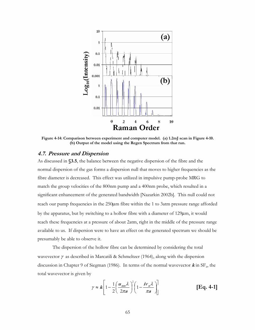
65
Figure 4-14: Comparison between experiment and computer model. (a) 1.2mJ scan in Figure 4-10. (b) Output of the model using the Regen Spectrum from that run.
4.7. Pressure and Dispersion As discussed in §3.5, the balance between the negative dispersion of the fibre and the
normal dispersion of the gas forms a dispersion null that moves to higher frequencies as the
fibre diameter is decreased. This effect was utilized in impulsive pump-probe MRG to
match the group velocities of the 800nm pump and a 400nm probe, which resulted in a
significant enhancement of the generated bandwidth [Nazarkin 2002b]. This null could not
reach our pump frequencies in the 250µm fibre within the 1 to 3atm pressure range afforded
by the apparatus, but by switching to a hollow fibre with a diameter of 129µm, it would
reach these frequencies at a pressure of about 2atm, right in the middle of the pressure range
available to us. If dispersion were to have an effect on the generated spectrum we should be
presumably be able to observe it.
The dispersion of the hollow fibre can be determined by considering the total
wavevector γ as described in Marcatili & Schmeltzer (1964), along with the dispersion
discussion in Chapter 9 of Siegman (1986). In terms of the normal wavevector k in SF6, the
total wavevector is given by
−
−≈a
i
a
uk nnm
πλν
πλ
γ 122
11
2
[Eq. 4-1]

66
In the equation, nmu is the mth root of the ordinary Bessel function of order n – 1 (since the
hollow fibre contains the beams in its fundamental hybrid mode, n and m will both equal
1), a is the inner radius of the hollow fibre, λ is the wavelength of the light, and nν is an
effective index of refraction of the guiding material (in this case fused silica), which is given
in terms of its normal index of refraction ν by
( )12
12
2
−
+=
ν
νν n [Eq. 4-2]
Note that γ is a complex-valued function, where its real part describes the dispersion and its
imaginary part gives the fibre attenuation. The nth order dispersion is then determined by
taking the nth order derivative of the real part of γ with respect to frequency – the effects of
various orders of the dispersion are illustrated in Figure 3-3.
If the dispersion was to have an effect on the generated MRG spectrum, it should be
readily observed by comparing the effect of intensity and pressure, as they should both
equally affect the strength of the nonlinearity in the absence of dispersion. The first
experiment was therefore to compare what happens when the energy was reduced by half
relative to when the pressure was halved. In keeping with our findings in the intensity scan,
we avoided self-phase modulation on the pumps by stretching the 383THz and 360THz
pulses to approximately 550fs. The energy was balanced between the two beams, but was
considerably lower than obtained earlier, where each pulse contained an energy of ~0.4mJ. I
chose not to maximize the energy, as this was the first experiment with the smaller fibre and
I wanted to avoid damaging it as much as possible. However, even without our maximum
energy the results of were spectacular – as can be observed in Figure 4-15, a significant
difference between halving the pressure versus halving the energy was observed even on a
logarithmic scale. By halving the pressure from three atmospheres to one and a half, the
intensity of the generated spectrum experiences a huge enhancement in the higher anti-
Stokes orders, which is opposite to what would be expected if the dispersion did not affect
the spectrum.

67
Figure 4-15: Demonstration of how dispersion affects transient MRG.
To further investigate the effect of dispersion and the occurrence of the complex
structure on the peaks, a detailed pressure scan was conducted, where just like in §4.3, the
pressure was reduced in increments of 5psi (with an extra scan at 1atm + 7.5psi from Figure
4-15). The dramatic results of this scan are compiled in Figure 4-16, where the spectra as a
function of pressure is plotted on a linear scale. While the initial MRG spectrum at three
atmospheres was modest compared to earlier results, as the pressure was decreased down to
one atmosphere a number of orders grow to become comparable to the pump beams – even
surpassing the transmitted long-wavelength pump beam in intensity! This enhancement was
not observed when the 250µm fibre was used (see the pressure scan of Figure 4-7), again
highlighting the importance of the dispersion in the smaller fibre.
Figure 4-16: Dependence of the spectra with pressure on a linear scale. The pressure scale is decreasing into the page.

68
Further details can be observed in Figure 4-17, where the individual spectra from this
same scan are plotted on a logarithmic scale. It is interesting that the spectrum at first
retreats as the pressure is reduced, but then around two atmospheres becomes successively
broader, with intensities that are far enhanced compared with the original 3atm case and
with orders that grow a broad red-shifted shoulder. One might attribute these shoulders to
self-phase modulation, however contrary to what one would expect this broadening is largely
absent at both the highest pressure and on the more intense pump beams. Finally, the
manner in which the orders broaden – into a red-shifted shoulder with a number of peaks –
is inconsistent with the normal idea of SPM, where the broadening depends on the
derivative of the intensity and as such should generate both a red-shifted and blue-shifted
wing due to the leading and trailing edge of the pulse respectively. That is, they are
inconsistent with the idea of SPM from a symmetric pulse, but could potentially be explained
by the formation of a pulse that has a sharp front edge and a gentle trailing tail.
Figure 4-17: The dependence of the generated spectrum with pressure on a logarithmic scale, where
the pressure for each spectrum is given in the top right-hand corner.

69
To get a sense of the dispersion we chose to consider the group delay, which was
used in §3.5 to get a sense of the dispersion characteristics of a hollow fibre. Again, it is a
measure of the delay one frequency experiences relative to another, and is inversely related
to the group velocity. Plotted in Figure 4-18 is a reproduction of Figure 4-17 overlaid with
the group delay, which is taken relative to the minimum group delay in the frequency range
of the plots. The only clear correlation between the spectrum and the group delay is that the
enhancement lies within a range where the group delay is less than 40fs/m. Put another
way, given that the fibre is about one metre long, the broadened and enhanced Raman
orders are only evident when they have been delayed with respect to one another by less
than a vibrational period, which is 43fs for the A1g vibration of SF6. It is likely that the
enhanced bandwidth is simply due to the fact that the orders do not walk off the pump
beams as much during their propagation. This however would not explain the complex red-
shifted shoulders on the Raman orders themselves.
Figure 4-18: A reproduction of Figure 4-17 overlaid with a plot of the group delay relative to the short-
wavelength pump.
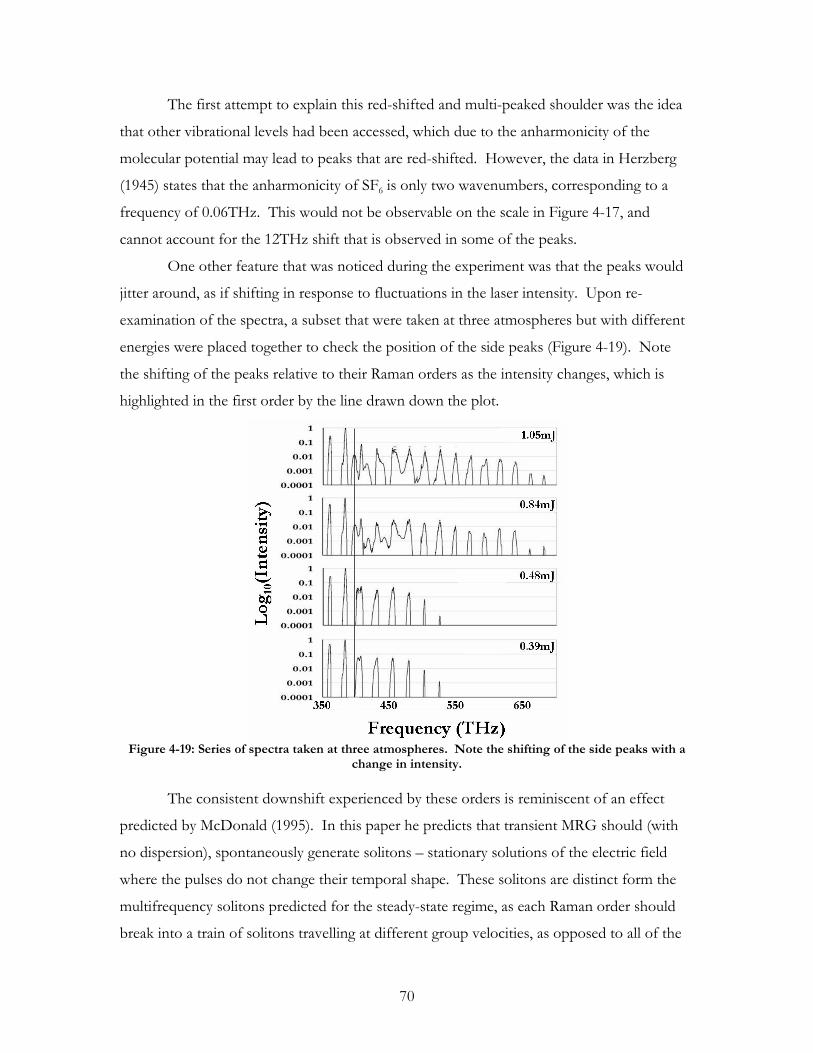
70
The first attempt to explain this red-shifted and multi-peaked shoulder was the idea
that other vibrational levels had been accessed, which due to the anharmonicity of the
molecular potential may lead to peaks that are red-shifted. However, the data in Herzberg
(1945) states that the anharmonicity of SF6 is only two wavenumbers, corresponding to a
frequency of 0.06THz. This would not be observable on the scale in Figure 4-17, and
cannot account for the 12THz shift that is observed in some of the peaks.
One other feature that was noticed during the experiment was that the peaks would
jitter around, as if shifting in response to fluctuations in the laser intensity. Upon re-
examination of the spectra, a subset that were taken at three atmospheres but with different
energies were placed together to check the position of the side peaks (Figure 4-19). Note
the shifting of the peaks relative to their Raman orders as the intensity changes, which is
highlighted in the first order by the line drawn down the plot.
Figure 4-19: Series of spectra taken at three atmospheres. Note the shifting of the side peaks with a
change in intensity.
The consistent downshift experienced by these orders is reminiscent of an effect
predicted by McDonald (1995). In this paper he predicts that transient MRG should (with
no dispersion), spontaneously generate solitons – stationary solutions of the electric field
where the pulses do not change their temporal shape. These solitons are distinct form the
multifrequency solitons predicted for the steady-state regime, as each Raman order should
break into a train of solitons travelling at different group velocities, as opposed to all of the

71
orders becoming locked into a single train. The red-shifted peaks provide a hint that this
may be the case, as solitons in general experience a shift to lower frequencies [Gordon 1986].
While this frequency shift is not strictly intensity-dependent as observed in the experiment, it
does depend on the soliton pulse duration, which may in some way depend on the strength
of the MRG interaction. As well, while it has been shown that typical two-colour Raman
solitons are unstable with positive dispersion, the solitons predicted by McDonald (1995)
were described as being robust to phase dispersion and other complicating factors, and
indeed it was said that the nonlinear dynamics of transient MRG were strongly attracted to
this solution.
The final attempt at understanding the complex broadening of the orders was to
map the positions of the side peaks to the pressure, to see if there was a noticeable trend.
This was done by subjectively deciding where the peaks lay in the spectrum given their
proximity to one another. That is, if there was a single broad shoulder that had a flat top, it
was assumed that it consisted of two peaks, where because of their jittering during the
average they blended into one another. The peaks on the first few orders seemed to be
relatively stable in their position, and it was thought that the other peaks might also be
shifted by a definite amount. Their behaviour turned out to be more complicated than
expected as shown in Figure 4-20, and no clear pattern has yet been established. The
primary Raman orders are highlighted with arrows, and the way the peaks seemed to meld
into and away from each other as the pressure is changed is depicted by the curved lines
drawn on the plot.
Figure 4-20: Mapping of the position of the peaks with pressure. The arrows show the primary
Raman orders, and the pressure is on a scale that decreases as it goes up the page.

72
5. Concluding Comments It was the main goal of this research to determine the potential of this laser system for
producing few-cycle pulses. In the absence of an experimental demonstration, this potential
can be investigated using a numeric fast Fourier transform (FFT), which converts a discrete
intensity spectrum into a temporal profile. The choice of which spectra to use was
determined by considering how we expected to compress the resulting radiation. To
maintain high energies, and to avoid purchasing expensive optical devices such as a liquid-
crystal phase modulator, we opted to consider the compression setup described in Sokolov
et al (2001), where a series of prisms and delay lines were used to time up individual orders.
As such, only the truly discrete spectra – not those exhibiting strong SPM – were Fourier
transformed, even though the ones with SPM might give a more isolated pulse. These
Fourier transforms are given in Figure 5-1. In part (a), the 2.4mJ spectrum from the
intensity scan is Fourier transformed, yielding a central pulse with a duration of 3.2 fs and an
estimated energy of 120µJ. Part (b) gives the Fourier transform of the pump-probe
spectrum of Figure 4-6, which results in a central pulse that has a duration of 3.3fs and an
estimated energy of 14µJ. If these pulse energies could be obtained, they would be an order
of magnitude more energetic than comparable pulses generated using other techniques, such
as the 25µJ, 3.8fs pulse synthesized using continuum generation [Steinmeyer 2006], and the
1.5µJ, 3.8fs pulsed synthesized using impulsive pump-probe MRG [Zhavoronkov 2002].
Figure 5-1: Fast Fourier Transforms. (a) The 2.4mJ MRG spectrum of Figure 4-10 and its FFT. (b) The pump-probe spectrum of Figure 4-6 and its FFT.

73
Along with the exhibiting the potential of transient MRG to generate high-energy
few-cycle pulses, this study has also discovered very exciting behaviours when examining the
generation in a system of low dispersion – behaviours that have not yet been reported in the
literature. The peculiar enhancement with decreasing pressure is likely to have implications
in how to optimize the apparatus to generate the largest bandwidth, and therefore synthesize
the shortest pulse. As well, regardless of whether the Raman orders are generating solitons,
there is sure to be some interesting physics to be discovered in the low-dispersion regime.
From this vantage, there are a number of direction which we intend to follow. First
and foremost we intend on further examining the behaviour of transient MRG in the small-
diameter fibre, with further experiments and the development of a comprehensive nonlinear
computer model. As well, we have been developing a system similar to that described in
Sokolov et al (2001), where we will use a system of prisms and delay lines to compress the
pulses, and use the ionization signal of a noble gas in a time-of-flight chamber to measure
the pulse duration. Another potential study is testing the growth of the MRG bandwidth
with the propagation distance, by using a number of shorter hollow fibres. In the
experiment it was consistently noticed that significant Raman generation was occurring
within the first few centimetres of propagation, as the small amount of light that leaked out
of the fibre looked as white as the output beam. With the realization of that experiment, we
can investigate the growth of MRG independent of both dispersion and the other nonlinear
effects such as self-phase modulation, and compare that to both an energy and pressure
study.
With the experience gained throughout this study and the many areas of research
that are now left open to us, the study of transient multifrequency Raman generation is sure
to continue to have a rich future at the University of Waterloo.

74
Appendix A: Modelling the Regenerative Amplifier While the core of this research is presented in sections one through five, as is usually the
case there was a significant amount of supplemental work required for the development of
this study. To outline the details for future reference, it has been organized into a series of
appendices, where appendices A and B focus on the practical parts of daily lab work,
including how to model, build, and align optical systems, and appendix C contains a
transcript of the final computer code used in the simulations.
This appendix will primarily deal with modelling physical optical systems, with
particular attention to designing a regenerative amplifier. Much of this discussion will be in
reference to two particular textbooks: Anthony E. Siegmans Lasers, and Orazio Sveltos
Principles of Lasers [Siegman 1986; Svelto 1998]. However, a slightly modified notation is used
for the sake of clarity.
The effort to model the Regen began after the regular occurrence of damage on the
crystal, and occasionally one of the back mirrors. The first thing to be determined was
whether changing the focal length of one of the curved mirrors from 50cm to 100cm might
solve the problem, keeping in mind that damage to the Pockels Cell must be avoided at all
cost. The effect of other parameters was to be studied as well, to determine if there might
be a more suitable design. In the end, it was decided that switching the mirror was not
practical, but that along with some minor adjustments to various lengths in the cavity, the
problem should be solved simply by moving the crystal further from the focus of the cavity
mode.
A.1 ABCD Matrices One of the formalisms used to describe the propagation of light is that of ABCD or Ray
Matrices. As the name implies, it uses a geometrical description of light rays in the form of a
matrix to model the action of an optical element on a wavefront. It begins by considering
the propagation of a ray of light through a general optical element such as in Figure A-1.
The incident ray is labelled 1rρ and the ray transmitted ray is labelled 2r
ρ. The ABCD matrix
for this optical element describes the effect of that element on the distance ( )d , and
direction
∂∂z
d of the ray relative to the optical axis. In general, it is assumed that there is a

75
linear relation between the distances and directions of the input and output rays. These
linear relations are given by
112
112
dDdCd
dBdAd
′⋅+⋅=′
′⋅+⋅= [Eq. A-1]
where zdd ∂∂=′ . These equations can be then be rewritten as
1
1
1
2
2
2 rMd
d
DC
BA
d
dr
ρρ⋅=
′
⋅
=
′
= [Eq. A-2]
where M is the ABCD matrix of the element. An important property of these matrices is
that in free space, the behaviour of the optical element should simply be reversed when
sending the beam back through the other direction, thus the determinant of the matrix
BCAD − is equal to 1 (with two separate materials on either side of the element, the
determinant is equal to the ratio of their indices of refraction).
Figure A-1: Action of a general optical element on a ray of light
The particular choice of using d and d ′ to describe the vector r
ρ is not arbitrary. A
key attribute of an optical wavefront is the radius of curvature R , which in the paraxial
approximation can be written as ddR ′= . In the case of a spherical wave the radius of
curvature can completely describe its propagation, and as such it is useful to consider the
change in R as a wave propagates through an optical element. Assuming a wave of with a
radius of curvature '111 ddR = , the new radius after propagation through a general optical
element is found to be
DRC
BRAR
+⋅
+⋅=
1
12 [Eq. A-3]
. As an example of how to construct one of these ray matrices, consider the passage of
a ray of light starting in vacuum and going through a dielectric block of length L and index
of refraction n (Figure A-2). By Snell’s Law,
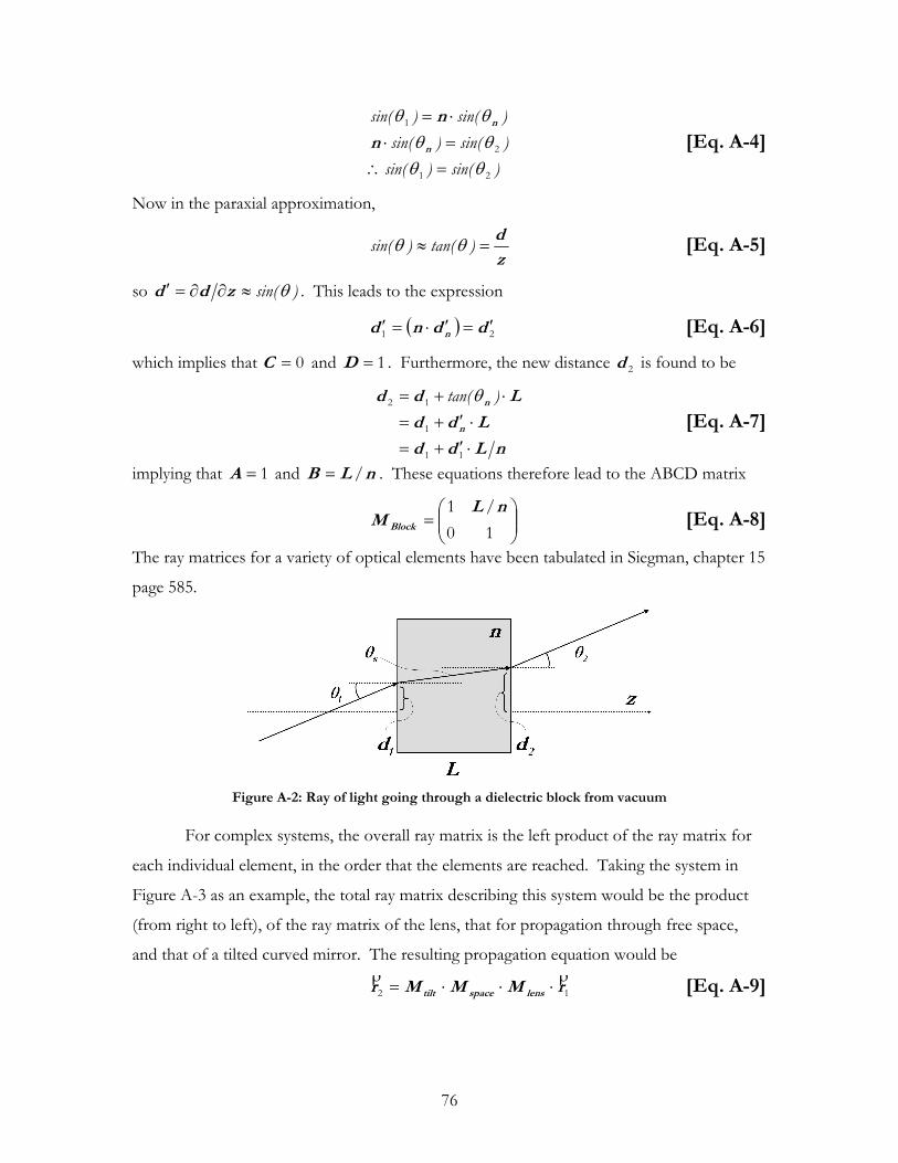
76
)sin()sin(
)sin()sin(
)sin()sin(
21
2
1
θθθθθθ
=∴
=⋅
⋅=
n
n
n
n
[Eq. A-4]
Now in the paraxial approximation,
z
d=≈ )tan()sin( θθ [Eq. A-5]
so )sin(θ≈∂∂=′ zdd . This leads to the expression
( ) 21 ddnd n′=′⋅=′ [Eq. A-6]
which implies that 0=C and 1=D . Furthermore, the new distance 2d is found to be
nLdd
Ldd
Ldd
n
n
⋅′+=
⋅′+=
⋅+=
11
1
12 )tan(θ [Eq. A-7]
implying that 1=A and nLB /= . These equations therefore lead to the ABCD matrix
=
10
1 nLM Block
/ [Eq. A-8]
The ray matrices for a variety of optical elements have been tabulated in Siegman, chapter 15
page 585.
Figure A-2: Ray of light going through a dielectric block from vacuum
For complex systems, the overall ray matrix is the left product of the ray matrix for
each individual element, in the order that the elements are reached. Taking the system in
Figure A-3 as an example, the total ray matrix describing this system would be the product
(from right to left), of the ray matrix of the lens, that for propagation through free space,
and that of a tilted curved mirror. The resulting propagation equation would be
12 rMMMr lensspacetilt
ρρ⋅⋅⋅= [Eq. A-9]

77
Figure A-3: Propagation through multiple optical elements
A.2 Gaussian Beams While these ray matrices can completely describe the propagation of a spherical wavefront,
in the laboratory one typically uses a laser beam, which has a Gaussian profile instead of a
spherical one. Fortunately, Gaussian beams can be treated in a way that is exactly analogous
to that of spherical waves. To help motivate the discussion, consider first the mathematical
representation of a paraxial spherical wave propagating in the z-direction. By saying the
wave is paraxial, it is assumed that we are considering only those points in space where the
distance ρ from a source at the origin can be written as
z
yxz
2
22 ++≈ρ [Eq. A-8]
which in turn allows one to write the electric field as
( )( )
( ) ( ) ....,~
cceezEcce
tE tkziR
yxiktki
+⋅⋅≈+= −−
+−−−
ωωρ
ρρ 2
22
[Eq. A-9]
In this approximation, the radius of curvature is approximately equal to z (instead of as a
function of x , y , and z ). Taken literally, this form of the electric field is infinite in extent
along the x and y directions, which is not physically realistic (starlight being the only
possible exception). A Gaussian beam is modified by having a finite beam waist w in the
directions transverse to that of propagation, such that the electric field can be described as
( ) ( ) ..)(,,,~
cceeezEtzyxE tkziR
yxik
w
yx
+= −−
+−
+−
ω2
22
2
22
[Eq. A-10]
Note how the new exponential factor is real-valued. Bringing this into the transverse phase
factor, one can define a new complex radius of curvature q to put the equation in the form
( ) ( ) ..)(,,,~
cceezEtzyxE tkziq
yxik
+= −−
+−
ω2
22
[Eq. A-11]
where q is found to be
22
1
2
1
kw
i
Rq−= [Eq. A-12]

78
The resulting expression [Eq. A-11] looks exactly like that of a spherical wave [Eq. A-9] with
R replaced by q . A Gaussian beam can then be modelled using ray matrices in exactly the
same fashion as a spherical wave by replacing R with q everywhere in [Eq. A-3].
A number of insights can be found by considering the propagation of a Gaussian
beam using ray matrices. Consider for example an initially collimated beam, such that the
radius of curvature is infinite and it has an initial size 0w as in Figure A-4. In this case
2
00
1
w
i
q πλ
−= [Eq. A-13]
(note that k has been replaced by its free-space value λπ2 ). Rearranging [Eq. A-3], one
can find the new q after propagating a distance z as
0
01
qBA
qDC
q z +
+= [Eq. A-14]
where
=
10
1 z
DC
BA [Eq. A-15]
is the ray matrix for propagating in free space. With some manipulation, one can find
expressions for the new beam waist and radius of curvature
+⋅=
+=
22
40
22
20
0 11z
wzR
w
zww
λπ
πλ
; [Eq. A-16]
As is demonstrated in Figure A-4, this implies that a Gaussian beam cannot maintain a
particular finite beam waist indefinitely. This leads to the idea of the Rayleigh range, which
is the length that it takes an initially collimated beam of initial 0w to expand to a size of
02 w⋅ , which is λπ 2
0wz R = . This is standard measure of how long a beam will remain
collimated. As an example, a typical beam in our laboratory will be 1cm in diameter with a
wavelength of 800nm, and so will remain collimated for approximately 100 metres.

79
Figure A-4: Propagation of a Gaussian beam through a distance z in free space.
Another derivation that is particularly useful is the spot size of a Gaussian beam after
going through a thin lens. Assuming a collimated beam, the beam would first go through a
lens and then propagate a distance z through free space, such that the overall ray matrix
would be
−
−=
−
⋅
=⋅=
11
1
11
01
10
1
f
zfz
f
zMMM lensspacetotal [Eq. A-17]
leading to a complex radius of curvature
2
0
2
0
1
11
wzifz
wif
q πλπλ
−−
−−= [Eq. A-18]
To find where the beam is focussed, we set the real part equal to zero, giving
4
0
222
4
0
2
wf
fwz
πλπ+
= [Eq. A-19]
In the usual case where 2
0wf πλ << , this turns out to be the focal length f as expected..
Plugging in fz = into the imaginary part of q1 we can find the beam waist* after
focussing with a lens
0w
fw
πλ
≅ [Eq. A-20]
A.3 Modelling a Laser Cavity When modelling the Regen cavity, it is to ones advantage that the lowest order transverse
mode of a cavity mode is that of a Gaussian distribution. While higher-order transverse * Note that this equation and many others found in the literature assumes that the beam waist is defined as the radius at which the field has dropped to e1 of its maximum value. I don’t know how
many times I’ve mucked up an intensity calculation by using the statistical Gaussian distribution 22 2wre − , or
had forgotten to switch the beam waist from the waist of the field to that of the intensity (which is the field
squared, yielding a new beam waist which is 2 smaller than the field waist).

80
modes can be generated due to damage or obstacles in the cavity, it is usually only the TE00
that is excited. As such, it becomes convenient to model the cavity by using simple ray
matrices, with a few rules governing the propagation of the beam as it oscillates in the cavity.
The most important of these rules is that, to be a stable cavity mode, the wavefront
must be self-consistent. That is, it must repeat itself after a full round trip so that
initial
initial
initialfinal qBA
qDC
qq +
+==
11 [Eq. A-21]
where the ABCD matrix is formed by the left product of the individual ray matrices as the
wavefront traverses the cavity. The model used to determine the round-trip ray matrix
(shown in Figure A-5(b)), is a simplified version of the actual Regen shown schematically in
Figure A-5(a). The changes are as follows:
1. For the purposes of the model, the Pockels Cell, crystal, and prisms only affect
the optical path length the light has to go through, so these have been absorbed into
the lengths 1L , 2L , and 3L .
2. The curved mirrors are modelled as lenses, where 2MirrorRf = . Astigmatism is
considered by modelling the modes in the both the sagittal and tangential directions
(see the ray matrices in Siegman (1986)).
3. The extra positions of 1z , 2z , and 3z are added to help determine the cavity
mode at any point within the cavity.
The round-trip ABCD matrix is then found by following the path depicted in Figure A-5(b):
11112222333
2322111
ZZLLensZZLLensZZL
MirrorLLensLLensLMirrorTripRound
MMMMMMMM
MMMMMMMM
⋅⋅⋅⋅⋅⋅⋅⋅
⋅⋅⋅⋅⋅⋅=
−−−
− [Eq. A-22]
Figure A-5: Modelling the Regen. (a) Schematic of the Regen. (b) Simplified model.

81
The elements in the round-trip ray matrix can then be used to generate the self-
consistent solution. Eq. A-21 can be rearranged to form
q
DC
q
B
q
A+=+
2 [Eq. A-23]
where the subscripts have been dropped. By using the fact that the determinant
( ) 1=−= BCADMdet when an optical element is in free space, one can obtain the
solution
2
21
2
1
+
−±−
=DA
B
i
B
AD
q [Eq. A-24]
Now for this solution to be realistic, it must follow two other criteria. Firstly, it must
be a confined solution, such that is has a finite beam waist. This implies the solution must
have a negative imaginary component as ( ) 21 wq πλ−=−Im . The condition can be
quantified by inspection of the solution [Eq. A-24]. If all the matrix elements are real, the
condition that the mode be confined simply requires
12
2
2
<=
+
mDA
[Eq. A-25]
and that one choose the appropriate solution for q1 . While in general the matrix elements
can be complex-valued, in practice they are not unless one includes the radially decreasing
gain in the Ti:Sapphire crystal. This acts to stabilize the cavity mode – permitting lasing even
if the cavity is geometrically unstable. This effect is neglected in the final calculations as it
makes them unnecessarily complicated, plus a test of the program with and without this
effect could not determine a difference between the two situations.
The other condition is that the solution must be perturbation-stable. To be
perturbation-stable simply means that if the wavefront is slightly different than that of the
cavity solution [Eq. A-24], the small deviations from this solution should decrease with each
round trip. This is similar to the difference between the stable equilibrium of a damped
pendulum, and the unstable equilibrium of a pencil balanced on its head. Mathematically,
assume a cavity solution CCavity qq = , then if one actually starts with a beam where
11 qqq C ∆+= , after one round trip the new complex wavefront curvature

82
2
1
12 qq
DCq
BAqq C ∆+=
+
+= [Eq. A-26]
should be such that 12 qq ∆<∆ . An analytical condition can be found by replacing 1q
into 2q , making the assumption that qq <<∆ , and removing Cq from both sides of the
resulting equation. This gives
2
22
1
2 122
λ≡
−
++
=∆
∆ DADA
q
qµ [Eq. A-27]
where the sign is opposite to the corresponding solution in Cq determined from [Eq. A-24].
λ corresponds to the eigenvalues of the ABCD matrix, and is often termed the perturbation
eigenvalue, even though the perturbations actually grow as 2λ . With real matrix elements,
2m must be less than 1 or the deviations from the cavity solution will simply grow in time.
While this is basically the same criterion for having a confined cavity mode, the difference
becomes apparent when the matrix elements are complex, as the element B is present in
[Eq. A-24] but not in the perturbation eigenvalues, so a confined but unstable solution is
possible (again, much like a pencil on its head – the solution exists, but is unstable).
A.4 Results of the program The entire purpose of modelling the Regen was to help determine whether we could replace
one of the curved cavity mirrors, so the first step was to determine the cavity mode with the
Regen as it was. The parameters of our Regen were as follows (see Figure A-5 and follow
from the first plane mirror): cmL 291 = , o151 =θ , mRMirror 11 = , cmL 5782 .= ,
mRMirror 502 .= , o152 =θ , and cmL 5643 .= , where the folding angles θ1 and θ2 are the
angles between the crystal arm and the Pockels Cell and Prism arm respectively. This led to
the cavity mode in Figure A-6. To switch the second curved mirror to a 1m mirror, different
parameters needed to be chosen to maximize the size of the beam at the Pockels Cell within
realistic limits for the size of the Regen given our workspace. The cavity mode in Figure A-7
was obtained using parameters of cmL 501 = , cmL 1022 = , and cmL 903 = . Note that
while the size of the mode was found to increase as the value of 2L decreased, the cavity
mode quickly became more unstable. As a compromise, 2L was chosen to be at least 1 inch
away from the point where the cavity would be completely unstable.

83
Figure A-6: Cavity mode in the present Regen with astigmatism included. The solid line is the tangential cavity mode, the dotted line is the sagittal cavity mode, and the dashed line is the pump
beam entering the cavity through the second curved mirror.
Figure A-7: Cavity mode when the 50cm curved mirror was replaced by a 1m. The solid and dashed lines are as described in Figure A-6.
Comparing the graphs in Figure A-6 with Figure A-7, the first thing to notice is that
while the beam size is better at the second plane mirror, the beam size at the Pockels Cell
has decreased significantly, which is definitely not acceptable. As well, the Regen would be
operating close to the edge of unstable operation making its operation tricky. Finally the
physical dimensions would be significantly larger, necessitating the rearrangement of
practically the entire optical bench. As the damage to the crystal had been remedied simply
by moving the crystal away from the focus during the development of this program, the
switching of the mirror was deemed unnecessary. However, having developed a program
that could look a the behaviour of the Regen, it was interesting to get a sense of how it
behaved as a function of the lengths between different optical elements 1L , 2L , and 3L .
The crucial details to pay attention to were again the perturbation-stability
determined by 2m , and the energy densities at the mirrors and in the Pockels Cell. While

84
the plane mirrors should be able to withstand between 1 and 3J/cm2, the focussing mirrors
and Pockels Cell would damage above 1J/cm2. The peak energy density was calculated by
assuming it followed a form much like the intensity: a Gaussian profile where the beam waist
w marks the 21 e point. The spatial integral over energy density
∫∫∞ −
⋅⋅⋅0
2
0
2
0
2
2
drreDd w
rπ
θ [Eq. A-28]
should then equal the total energy in the pulse. This yields the relation
240
10
2
w
ED
π−= [Eq. A-29]
in J/cm2 when w is in metres. The plots of the energy density for the mirrors as a function
of 1L , 2L , and 3L are shown in Figure A-7, where the maximum energy in the cavity was
taken to be 5mJ. The legend follows the optical elements from the one experiencing the
highest energy density to that with the lowest, plus a plot of 2m where the magnitude of the
scale is the same, but the units are dimensionless. Note that the plots for the Plane Mirror
#1 and Lens #1 (Curved Mirror #1) overlap for all three graphs, and as such they also
describe the energy density at the Pockels Cell.
Figure A-8: Variation in the energy densities at various optical elements with the separations L1, L2, and L3. Note that the when plotting the Energy Density against one of the lengths, the other two are
kept at their nominal values of L1=29cm, L2=78.5cm, and L3=64.5cm
In terms of the flexibility in the design, the most restrictive condition seems to be
that on 2L – within a range of about 10cm the cavity mode can switch from being unstable
but having low energy densities on all the optics, to a point where it is incredibly stable but
the energy density is dangerously high on the second plane mirror. The other two distances

85
however can both be increased significantly, with an overall increase in mode stability and a
reduction in the energy density at the mirrors. Recalling that the damage thresholds for the
curved mirrors and Pockels Cell are ~1J/cm2, for the crystal and prisms ~5J/cm2, and for
the plane mirrors are between 1J/cm2 and 3J/cm2, it should be noted that for the current
design of the Regen plane mirror #2 is in danger of damaging. However, since none of the
other optical elements should damage, and as the damage to this mirror has been infrequent
(once every couple of months), the design has been pretty much left as it was, with any
successive adjustments made to the cavity tending to increase the distances 1L and 3L to
reduce the probability of damaging this mirror (as far as its allowed by the space on the
optical bench).

86
Appendix B: Alignment Some of the most valuable experience I’ve obtained working with ultrafast lasers have been
when things have broken down and needed repairing. However, the construction and
alignment of the different systems in the lab typically relied heavily on the advice of my
supervisor, with little supplementary documentation or illustration available to assist the
student. While the process of alignment is not difficult conceptually, it is one of the most
common and sometimes most frustrating tasks that a student encounters in a laser lab. This
appendix is designed to fill this gap somewhat by providing an account of the things I took
into account when building various optical setups, starting with general ideas for simple
optics, progressing to the alignment of more complicated elements such as the Pockels Cell,
and concluding with the construction and alignment of a Regenerative Amplifier. These are
some of the practical skills one must learn to be effective in the laboratory, and as such this
section will hopefully be an instructive guide for new students in the laser lab.
B.1 Plane Mirrors By far the most common element used in our lab, the alignment of plane mirrors is relatively
simple, yet can have some unexpected effects on the performance of an optical system. The
first thing to be considered is the design specifications of the mirror itself – the dependence
of the reflectivity on the angle of reflection, the polarization, and the wavelength. All of
these have a major impact on the throughput of a given system, especially given the ultra-
broad bandwidths that are produced in a femtosecond lab, and as such each mirror should
be labelled appropriately on its edge and a data sheet filed.
As a concrete example of why such care should be taken, our initial investigations
into MRG suffered from mirrors that had a very poor reflectivity at longer wavelengths.
Note that in the spectrum of Figure 4-1, the Stokes orders after the strongly saturated
845nm peak drop drastically, but produce a plateau on the linear scale. A plateau is normally
suggestive of the saturation of MRG, and as such should not be as weak as what was
observed (note that the saturated peaks are likely orders of magnitude stronger than shown
in the Figure, as they were very strongly saturating the detector). Using the wrong mirrors
was an oversight that contributed to significant delays in this experiment.
One thing that is affected by the alignment specifically is the polarization of the
beam. This is often exploited in periscopes to switch the polarization from p- (parallel)

87
polarized relative to the optical bench, to s- (perpendicularly) polarized relative to the optical
bench. The action of a periscope on the polarization is depicted in Figure B-2. In an
analogous way, combinations of mirrors that are angled away from the plane of the optical
bench can skew the polarization and thus affect things such as the transmission through the
experiment (see the P and S curves in Figure 4-1(b)). This is particularly significant when
using a pair of mirrors that are very close together, since they can be skewed at large angles
while still redirecting the beam in the right direction.
Figure B-2: All reflective polarization rotation
My final comment on the alignment of plane mirrors concerns aligning a beam into
an optical system using a pair of mirrors. As opposed to something on translation stages
where the alignment can be thought of in terms of a Cartesian “x and y” system, plane
mirrors lend themselves more to a polar “position and angle” sort of idea, since a single
mirror can only adjust the direction of a beam. With this sort of thinking, the mirror closest
to a given setup acts as the angle adjustment, while an earlier mirror acts as the position
adjustment. A system of two irises provides a convenient demonstration of this idea (Figure
B-3). While the position mirror does affect the angle of entry, and the angle mirror does
affect the position of the beam at the entrance of the system, these effects can be minimized
by placing the position mirror as far away from the system as possible (to maximize the
movement of the beam for a given adjustment in angle), and placing the angle mirror as
close to the system as possible (to minimize the movement of the beam for a given angle
adjustment). By iteratively adjusting the position and angle mirrors, one can quickly achieve
the desired alignment. Conversely, if one wants to set a pair of irises for future alignments,
the first iris should be placed as close to the angle mirror as possible, and the second iris
should be placed as close to the optical system as possible.

88
Figure B-3: Using plane mirrors for a Position-Angle alignment
B.2 Lenses Aligning a lens is relatively simple, as there are only a few things that need to be considered.
The first thing to note is that if the beam enters off-axis, it will be skewed towards the
opposite direction as it exits the lens. This can be avoided by setting a reference point for
the beam before the lens is in place, and adjusting the position of the lens to bring the beam
back on that reference.
For a short-focal-length lens where this may be difficult, one can take advantage of
the light reflected from the two surfaces of the lens. There will typically be one diffuse
(sometimes plane) reflection, and one focusing reflection as demonstrated in Figure B-4. To
see these reflections the lens will have to be slightly tilted to send them off-axis, where they
can be viewed on a card without interrupting the incoming beam. When the lens is moved
in the x and y directions, the relative positions of the reflections will change – the proper
alignment being when they lie one on top of the other. It is important that after any
alignment with the lens, these reflections should be sent into some sort of beam dump, or
better yet a diagnostic of the system. Otherwise, there is unnecessary stray light in the lab,
and there is the potential to damage other optical elements that may happen to be in the
focus of the second reflection.
Figure B-4: Aligning a lens. The diffuse (or possibly plane) reflection is from the front surface and is depicted in light grey. The focussed reflection is from the second surface and is in dark grey.

89
B.3 Prisms As the lasers used in this ultrafast lab typically lase at two colours simultaneously, many
systems use components such as prisms and gratings that spatially disperse the two colours.
This is used as a way of independently manipulating the beams, such as when selecting
colours or compressing the pulses. When using prisms, there are three major adjustments
needed for alignment – the angle of the prism relative to the beam, the tilt of the prism
along its length, and the tilt along its breadth (Figure B-5b, c, and d respectively). For the
principle angle alignment, a useful reference is the angle of least deviation. This is defined as
the angle at which the beam is deflected the least from its original path (see Figure B-5a).
This is important partly because the alignment is reproducible, and since the prisms are used
in pairs, for one to undo the action of the other the opposite faces must be parallel (this can
be thought of as a block of free-space placed at an angle within a block of material –
recalling that a block of material should not angularly disperse a beam of light. Try drawing
it if you don’t know what I mean). Two prisms can then be aligned by setting each one at
this angle of least deviation. As a convention, I approach this angle by rotating the prism
clockwise (if it were positioned as in Figure B-5a), until the front edge (long wavelength
edge), of the dispersed beam has stopped.
Figure B-5: Alignment of a prism. (a) Angular dispersion of a beam through the prism. (b) Primary angle adjustment. (c) Tilt of the prism along its length. (d) Tilt of the prism along its breadth.
The remaining two adjustments for the tilt of the prism affect the vertical deviation
of the transmitted and reflected beams. There should be two screws on the prism holders to
adjust these tilts. The tilt of the prism along its length (Figure B-5c) primarily affects the
alignment of the transmitted beam, whereas the tilt along its breadth (Figure B-5d) affects
both beams roughly equally. For alignment purposes then, one should start by adjusting the
tilt along the breadth of the prism to bring the reflected beam into alignment, and then
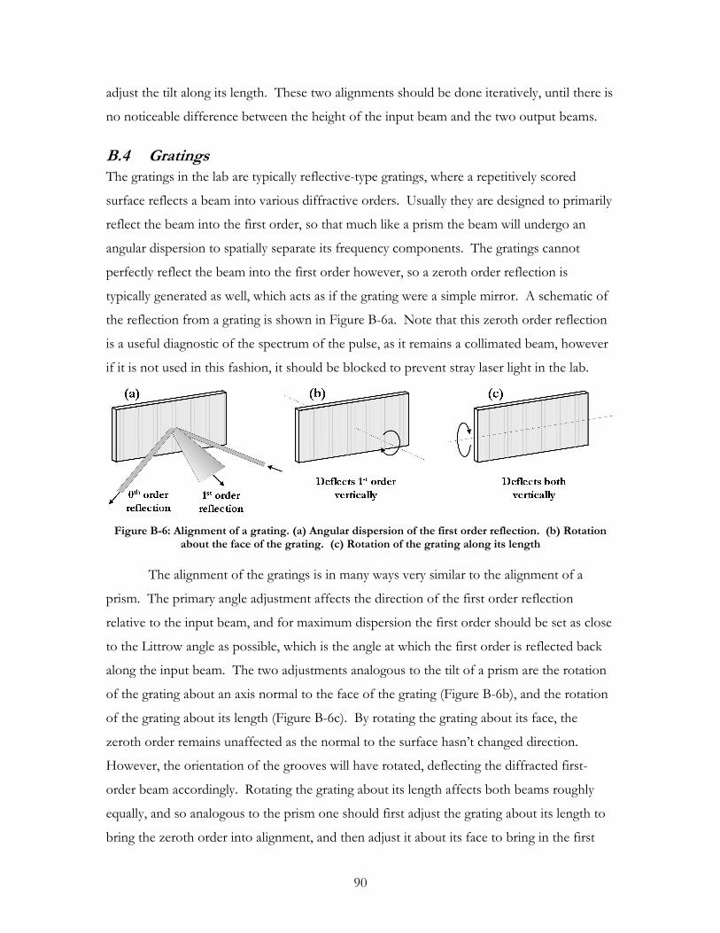
90
adjust the tilt along its length. These two alignments should be done iteratively, until there is
no noticeable difference between the height of the input beam and the two output beams.
B.4 Gratings The gratings in the lab are typically reflective-type gratings, where a repetitively scored
surface reflects a beam into various diffractive orders. Usually they are designed to primarily
reflect the beam into the first order, so that much like a prism the beam will undergo an
angular dispersion to spatially separate its frequency components. The gratings cannot
perfectly reflect the beam into the first order however, so a zeroth order reflection is
typically generated as well, which acts as if the grating were a simple mirror. A schematic of
the reflection from a grating is shown in Figure B-6a. Note that this zeroth order reflection
is a useful diagnostic of the spectrum of the pulse, as it remains a collimated beam, however
if it is not used in this fashion, it should be blocked to prevent stray laser light in the lab.
Figure B-6: Alignment of a grating. (a) Angular dispersion of the first order reflection. (b) Rotation about the face of the grating. (c) Rotation of the grating along its length
The alignment of the gratings is in many ways very similar to the alignment of a
prism. The primary angle adjustment affects the direction of the first order reflection
relative to the input beam, and for maximum dispersion the first order should be set as close
to the Littrow angle as possible, which is the angle at which the first order is reflected back
along the input beam. The two adjustments analogous to the tilt of a prism are the rotation
of the grating about an axis normal to the face of the grating (Figure B-6b), and the rotation
of the grating about its length (Figure B-6c). By rotating the grating about its face, the
zeroth order remains unaffected as the normal to the surface hasn’t changed direction.
However, the orientation of the grooves will have rotated, deflecting the diffracted first-
order beam accordingly. Rotating the grating about its length affects both beams roughly
equally, and so analogous to the prism one should first adjust the grating about its length to
bring the zeroth order into alignment, and then adjust it about its face to bring in the first

91
order. Note that since the grating mounts cannot be set perfectly the adjustments will not
be exactly along those axes, so they should be adjusted iteratively to bring the grating into as
good an alignment as possible.
B.5 Grating Compressor While the compressor in the lab compresses two beams simultaneously, it is sufficient to
consider the alignment for the case of a single-beam compressor. Following the path as
depicted in Figure B-7a, the incident horizontal beam travels over the top of the output
mirror, and is dispersed into the first grating order at an angle that is as close to Littrow as
possible (as close to going back on itself as possible). The beam is then re-collimated by
orienting the second grating so that the beam travels parallel to its original path. A mirror
reflects the beam back on itself, but with a slight tilt downward to aim the beam at the
output mirror placed below the incoming beam. The input beam and its retro-reflection
should then be vertically separated on the two gratings as in Figures B-7b and c.
Figure B-7: Alignment of a grating compressor. (a) Top view of a compressor. (b) & (c) Diagram of the beams on the first and second grating as seen through an IR viewer.
B.6 Pockels Cell The alignment of the Pockels Cell is a bit trickier than that of the simpler optical elements
described up to now. A Pockels Cell acts as an optical switch in a Regen cavity as it uses a
voltage-dependent birefringent wedge (the wedge shape helps prevent damage). When in
use, the birefringence is usually set to act as a quarter-wave plate when a voltage is off,
changing the polarization of the light that passes through it from linear to circular (this is
described in more detail in §3.2.1). The typical alignment procedure (known as the “Eye of
God” alignment), takes advantage of this affect on the polarization. The alignment setup
using the seed for our Regen is demonstrated in Figure B-8, where the Pockels Cell is the
box, in front of it is a linear polarizer with a diffuser (piece of tape), on the back is another
linear polarizer that is crossed with the first one, and the light is depicted in grey. Note that

92
we actually only have large circular polarizers in the lab, but in the proper orientation these
will act as linear polarizers. The alignment procedure is as follows:
1. Position the Pockels Cell without the polarizers in place so that the seed goes
through as well as possible. This may require lifting it vertically depending on the
optical axis of the cavity.
2. Place the polarizers on either side (without the diffuser), to get them crossed as
well as possible. This won’t be perfect so some seed will still get through, which will
actually become an asset later.
3. Place the tape on the front polarizer. When the Pockels Cell is aligned properly
this should give a circle of light with a dark cross in the centre, with an overall
surrounding ring of light. It should look like the left-most pattern in Figure B-8,
however without the central spot. If the seed were strong enough the spot would be
there, but the tape generally attenuates the beam to the point where this isn’t visible.
4. For the fine adjustment of the position, the dark cross and the central spot
should line up on each other. Since the spot isn’t visible with the tape in place, I
simply moved the polarizer back and forth to move the tape in and out of the beam.
5. For the angular alignment, the dark cross should line up with the broad
background circle of light (and forms a ring when properly aligned).
Figure B-8: “Eye of God” alignment for a Pockels Cell
As with all alignments, the last two steps may have to be repeated iteratively. Once
this is done, the Pockels Cell will act as a quarter-wave plate when the voltage is on, which is
opposite to the desired operation in the Regen. This can be remedied by using the

93
adjustment screws, which will be discussed in the section on building the Regenerative
Amplifier.
B.7 Building the Regenerative Amplifier There have been a few times that the Regen has needed to be rebuilt, usually after something
became seriously damaged (like the crystal), or its operation was substandard. When all the
mirrors and elements had been tweaked to no effect, the last resort was to take the Regen
apart bit by bit to find where the problem might be. The one time it was taken apart
completely was when we thought the pump beam was misdirected vertically, setting an odd
optical axis that was likely sending the infrared beam up and down throughout the Regen
cavity, possibly affecting the polarization and hence the cavity gain and losses. This
complete disassembly should be done truly as a last resort, as it is very time-consuming to
realign properly.
This section will present a particular way of constructing the Regen, but keep in
mind that there are many other ways of doing it, and this should really be used as a guideline.
The main thing to remember is that regardless of the procedure, when doing this alignment
only one optic should be adjusted at a time before setting some sort of reference. This is
to ensure that it’s possible to go back to an earlier configuration if a mistake is made.
B.7.1 Align the Pump Beam
The most important consideration for an amplifier is the overlap of the seed beam with the
pump beam, as there can be no amplification if there is no overlap. As such, it is the pump
beam that defines the optical axis of the laser, and so that is where the construction of the
Regen should start.
Initially, send the pump beam through its lens and the mirror that to this point has
been labelled the second curved mirror. Check to see that it is going flush to the table, and
then insert the crystal. Rotate the crystal about its length so that the reflection from the
front surface is also going flush to the table, and then rotate the crystal as shown in Figure
B-9, until the reflection at the front surface is minimized. The crystal will then be at the
Brewster’s angle, which is where p-polarized light experiences no reflection. Note that this is
slightly different than the Brewster’s angle for an IR beam, but it should be close enough.
Once this is done, the axis should be recorded using two irises, positioned such that they are

94
as close to either end of the cavity as possible, without getting in the way of the cavity mode
itself. The first curved mirror and a beam dump should also be in place.
Figure B-9: Alignment of the pump beam. The irises are a reference for the optical axis of the cavity.
B.7.2 Align the Polarizer and Curved Mirrors
The next step is to align the polarizer and mirrors using the seed beam. Position the
polarizer roughly where it should be, and use two redirecting mirrors (position and angle),
before the cavity as shown in Figure B-10 to direct the seed into the first curved mirror.
Using the first curved mirror and one of the redirecting mirrors, align the seed to the two
irises in the cavity. The alignment will probably not be perfect, as the deviation of the green
pump beam in the crystal will be slightly different than the deviation of the IR beam.
Figure B-10: Alignment of the curved mirrors
To set the alignment of the polarizer, use a half-wave plate to make the beam s-
polarized, which should be completely reflected by the polarizer when everything is aligned
correctly (depending on where the seed is taken from, it may already be s-polarized). Look
for a minimum in the transmitted beam when adjusting the polarization, as it is easier to find
than the maximum of the reflected beam. Note that both the reflection and transmission of
the beam through the polarizer should be flush to the table, and if they are not there should
be two adjustment screws on the polarizer mount. With the polarization set, determine the
optimal angle of the polarizer by rotating the polarizer and again finding the minimum in the
transmitted beam.
Once through the second iris, angle the second curved mirror towards a third plane
mirror, which for the time being will act as plane mirror #2 as shown in Figure A-5. Ensure

95
that the beam is flush to the table. This plane mirror should then be aligned to send the
beam back exactly on itself – this will be critical to get the Regen lasing later in the procedure,
and once this is set do not adjust it until it is up and lasing. To aid in this alignment, use
another iris as far back along the beamline as possible.
B.7.3 Align the Input of the Seed
With three of the four cavity mirrors set, ensure that the seed will keep this alignment when
it is injected by reflection off the polarizer. Using another iris to mark how it went into the
cavity in the previous step, reflect it off the polarizer and use a pair of mirrors earlier in the
beamline to bring it into alignment (Figure B-11).
Figure B-11: Setting the input of the seed as it will be used in regular operation.
B.7.4 Align the Last Cavity Mirror and the Pockels Cell
With the seed aligned, introduce the Pockels Cell into the cavity, and align it as
described in §B.6. Note that the Pockels Cell will currently be working opposite to what is
desired, as it will act like a quarter-wave plate with the voltage on. To remedy this, set up the
last cavity mirror as shown in Figure B-12, which was earlier called plane mirror #1. The
beam should be sent back on itself so that it again goes through the two irises in the cavity.
By introducing a fast diode in the path of the beam, it is possible to observe the effect of the
Pockels Cell on the seed, which can then be used to set it to the proper configuration.
Figure B-12: Alignment of the Pockels Cell using a diode.

96
When the Pockels Cell is working as a voltage-on quarter-wave plate, a diode placed
in the path of the seed will read a trace much like Figure B-13a, where the period between
the peaks is determined by the repetition rate of the oscillator. To interpret what is
happening, note that when the Pockels Cell is doing nothing, the s-polarized seed should
reflect off the polarizer, go through the Pockels Cell twice, and then again reflect off the
polarizer as the polarization should be the same. As the Pockels Cell cannot be set to have
exactly zero birefringence (and the polarizer may not be aligned perfectly), there will be some
light that leaks into the cavity, and therefore a small signal will be apparent. When the
voltage is turned on, the Pockels Cell should let almost all of the seed into the cavity by
changing it first to circular polarized light, and then to p-polarized as it is reflected back
through. When it is turned off again the signal should go back down. To get it to work in
the opposite configuration, adjust one of the screws at the back of the Pockels Cell (while
being careful of the high voltage line), to make the pattern switch from Low-High-Low to
Low-Low-High (or High-Low-Low). At this point, adjust the other screw until the pattern
becomes High-Low-High, as in Figure B-13c. The ratio of the peak heights should be 8:1 or
better.
Figure B-13: Typical traces from a fast diode when aligning the Pockels Cell. (a) Operation when it is acting like a voltage-on quarter-wave plate. (b) Intermediate stage by adjusting one of the alignment
screws. (c) Operation when it is acting like a voltage-off quarter-wave plate.
B.7.5 Remove the Diode and get it Lasing
With the diode removed from the cavity, it should be possible to get the Regen lasing. Try
to only use plane mirror #1 to bring the cavity into alignment, as it was aligned only by using
the irises, and if necessary it can be brought back to that alignment. If this does not work,
make sure that the output timing on the Pockels Cell is set to 100, so that the lasing is not
being cut off prematurely. If lasing is still not possible, plane mirror #2 can be adjusted.
Once the Regen is acting like a laser, iteratively adjust both of the plane mirrors to maximize
the energy in the pulses. Do not adjust the curved mirrors.

97
B.7.6 Insert the Prisms and finish the Alignment
To finish the Regen, the beam must be dispersed in the cavity to obtain a two-colour output.
This is done using a system of three prisms as shown in Figure B-14. Using again the angle
of least deviation as a reference, align the prisms as described in §B.3 to disperse the two
colours in the cavity. They must be well separated so that the colours can be spatially
dispersed enough to allow for two-colour operation. Adjusting only plane mirror #2, first
bring one colour and then the other back into alignment. The slits used for control of the
two colours can then be placed after the prisms, as can an optional attenuator using a
combination of a polarizer and a half-wave plate. This can be used to control the relative
energy between the two colours. With this done, you now have a two-colour regenerative
amplifier!
Figure B-14: Final alignment of the Regen.

98
Appendix C: Computer Code This is a transcript of the computer code used to model MRG. It was created in Matlab, and
as such any percent signs (%), are commented code, and are ignored in the program. These
are used to provide notes, or to switch back and forth from one variable to another.
clear; tic %%%%%%%%%%%%%%%%%%%% %Defining constants% %%%%%%%%%%%%%%%%%%%% %%Assume a value of the Raman gain - figure it out later g= 1.6e-13; c= 3e8; %%in m/s %%The Raman transition omegaRaman= 775; %%in wavenumbers dephasingTime= 6.6; %%in picoseconds HWHMRaman= .2206/(dephasingTime*1e-12)/3e10/2; %%in wavenumbers %HWHMRaman= 100; %%in wavenumbers convolution= 0; %%over what TOTAL range should a convolution be carried out in wavenumbers %% Note that a higher value is more accurate, but also much more taxing %% Also note that this will affect the value for g %%Define the fibre characteristics FibreLength= 1; %%in meters Intervals= 1000; %%number of points per meter; this number must be large for the program to work plotPoints= 1000; %%when plotting in 3d, it's best to have only 1000 points fibreRadius= 250; %%in microns Pressure= 3; %%in atmospheres u11= 2.405; %%zero of the Bessel function J[0](x) dz= FibreLength/Intervals; %%Define largest Stokes and Anti-Stokes order you want to include S_Orders= 20; %%including the long-wavelength beam A_Orders= 20; %%You can't interactively change the scale on a surface plot, so set the number you want to plot minorder= -S_Orders; %%use -S_Orders for all of them maxorder= A_Orders; %%use A_Orders for all of them %%Set the frequency resolution %%Note that a typical bandwidth is about 80 wavenumbers, so a spacing of 16 is appropriate omegaRes= 7; %%In wavenumbers %%Set the initial intensity of the Pump, and then the energy ratio between it and the Stokes Intensity= 6e12; %%in W/cm^2, but I don't think it matters, as g is a parameter to be determined ratio= 1.5; %%Finally, set the smallest intensity (relative to the Pump), that you want to plot plotmin= 1e-4; %%Labeling convention: short-wavelength beam (Pump beam) is order# S_Orders+3 %% long-wavelength beam (Stokes beam) is order# S_Orders+2 %%I'm adding two extra orders on either end for programming considerations Pump= S_Orders + 3; Stokes= S_Orders + 2;

99
toc %%%%%%%%%%%%%%%%%%%%%%%%%%%%%%%%%%%%%%%%%%%%%%%%%%%%%%%%%%%%%%%%%%%%%%%%%% %Determining resolution and constructing the input spectrum from our data% %%%%%%%%%%%%%%%%%%%%%%%%%%%%%%%%%%%%%%%%%%%%%%%%%%%%%%%%%%%%%%%%%%%%%%%%%% omegaIntervals= ceil(omegaRaman/omegaRes); %%number of intervals per order %%I'm going to make sure that there are an odd number of intervals per order. By forcing %% an odd number, I can define the array elements by using the orders as a reference. %% Notice how in the diagram below there are two points on either side of each order %% when there's 5 intervals per order. %% ..|....|....|....|....|.. %%Equivalently, the # of side elements = (# of intervals - 1)/2 %%The pump frequency is therefore at an index of (Pump Order)*(elements/order) %% - the bit on the side %% ..|....|....|....|....|....|....|.. %% 1 ^n ^2n ^3n ^Pump*n the arrows point to the element in question %% n=5, Pump Order=3, S_orders=1, A_orders=1, bit on the side=2 if (mod(omegaIntervals, 2)== 0) omegaIntervals= omegaIntervals + 1; end side= (omegaIntervals - 1)/2; %%This now sets the actual resolution, which will be as good as or better than %% the specified resolution omegaRes= omegaRaman/omegaIntervals; %%Read in the Regen Spectrum path(path, 'C:/Documents and Settings/Compaq/My Documents/Frasers/Frasers Junk/Waterloo/Work/MRG/Data/Data Analysis/mrg104_308_AND036-AND064'); [lambdaReg, IntensReg]= textread('AND064.mat', '%f %f', 'expchars', 'E', 'commentstyle', 'matlab'); omegaReg= 1e7./lambdaReg; RegenSpec= zeros(length(omegaReg), 2); RegenSpec= [omegaReg IntensReg]; %I'm artificially subtracting the background, as I didn't take one to begin with. RegenSpec(1: length(omegaReg), 2)= sqrt((RegenSpec(1: length(omegaReg), 2) - 9e-7).^2); RegenSpec(1: length(omegaReg), 2)= sqrt((RegenSpec(1: length(omegaReg), 2) - 3.5e-7).^2); RegenSpec(1: length(omegaReg), 2)= sqrt((RegenSpec(1: length(omegaReg), 2) - 1.75e-7).^2); RegenSpec(1: length(omegaReg), 2)= sqrt((RegenSpec(1: length(omegaReg), 2) - 0.9e-7).^2); RegenSpec(705: length(omegaReg), 2)= 0; RegenSpec(220: 620, 2)= 0; RegenSpec(1: 70, 2)= 0; %%Determine the frequency spacing points= length(omegaReg); range= omegaReg(1) - omegaReg(points); dOmegaReg= range/points; %%Determine the desired index spacing from the specified resolution. This should %% give a resolution that is as good or better than that specified spacing= floor(omegaRes/dOmegaReg); omegaRes= spacing*dOmegaReg; RegIntervals= floor(points/spacing); %%number of intervals over entire Regen range %%This is an example of what the array could look like; this time the lines are %% showing the array elements we want to keep %% |........|........|........|.... "points= 32, spacing= 9, intervals= 3" %% 1^ 9+1^ 2*9+1^ 3*9+1^ 32^ Listing the index at the arrow %%Now to get rid of all the extraneous points. Follow the diagrams above and below

100
%% |........|........|........|.... %% |........|........|........| %% ||........|........| %% |||........| %% |||| RegenSpec((spacing*RegIntervals + 2): points, :)= []; for n= 1: RegIntervals RegenSpec(1 + n: spacing + n - 1, :)= []; omegaReg(1 + n: spacing + n - 1, :)= []; end %%Now to set the ratio between the pump and the Stokes. We measure energy, so integrate %% the two peaks in the spectrum and determine the ratio of the areas. [pumpmax, pumpindex]= max(RegenSpec(:, 2)); omegaPump= omegaReg(pumpindex); RegenSpec(:, 2)= RegenSpec(:, 2)./pumpmax; %normalize the array to the Pump intensity StokesArea= 0; PumpArea= 0; %%In the original file, the Stokes beam is between the 70th and 220th data point, %% and the Pump beam is between the 570th and 710th data point for n= floor(70/spacing): ceil(220/spacing) StokesArea= StokesArea + (RegenSpec(n, 2) + RegenSpec(n - 1, 2))/2; end for n= floor(570/spacing): ceil(710/spacing) PumpArea= PumpArea + (RegenSpec(n, 2) + RegenSpec(n - 1, 2))/2; end SpectraRatio= PumpArea/StokesArea; scale= ratio/SpectraRatio; RegenSpec(floor(70/spacing): ceil(220/spacing), 2)= RegenSpec(floor(70/spacing): ceil(220/spacing), 2)... ./scale; %%Initialize the Frequency and Intensity arrays %%I'm adding a couple extra orders on either end as it's needed later omega= (omegaPump - (omegaIntervals*(S_Orders + 2) + side)*omegaRes: omegaRes: ... omegaPump + (omegaIntervals*(A_Orders + 2) + side)*omegaRes); %%Translation: Start at the centre, go back by ((the number of Stokes orders + two extra) %% *(number of array elements per order) plus the bit on the side), %% increment by the frequency resolution until you get to (Pump + Anti-Stokes + %% two extra orders), then add the number of elements on the side In= zeros(1, length(omega)); for n= pumpindex: length(RegenSpec(:, 2)); In(Pump*omegaIntervals - side - n + pumpindex)= RegenSpec(n, 2); end for n= 1: pumpindex - 1; In(Pump*omegaIntervals - side + n)= RegenSpec(pumpindex - n, 2); end %GVD= 0000e-6; %%I've set it to 10000; for Steve it was -1877 %TOD= 000000e-9; %%I've set it to 1000000; for Steve it was 18719 %extraphase= GVD/2.*(omega*100*3e8*2*pi).^2 + TOD/6.*(omega*100*3e8*2*pi).^3; %lambda= 1e4./omega; %%this gives the wavelength in microns toc %%%%%%%%%%%%%%%%%%%%%%%%%% %Set the phase dispersion% %%%%%%%%%%%%%%%%%%%%%%%%%% ngas= zeros(1, length(omega)); k= zeros(1, length(omega)); %ngas= ngas + 1; %%comment what's below to set no dispersion

101
%%Sellmeier equations for the gas ngas= 1 + Pressure*0.7e30./((31.9e15)^2 - (2.*pi.*c.*100.*omega).^2); %%from physrevA68_023812p15_2003 %%Sellmeier equation for fused silica %nsilica= sqrt(1.2955 + 0.80985*lambda.^2./(lambda.^2 - .0107945) + ... 0.91714*lambda.^2./(lambda.^2 - 100)); nsilica= 1.5; n1= (nsilica.^2 + 1)./(2.*sqrt(nsilica.^2 - 1)); %%Axial wavevector for the EH11 hybrid mode k= 2.*pi.*omega.*100.*ngas.*(1 - 1/2.*(u11./(omega.*100)./(2.*pi.*fibreRadius)).^2).*(1 - i*n1./(omega.*100)/pi/fibreRadius); %%%%%%%%%%%%%%%%%%%%%%%%%%% %Electric Field Amplitudes% %%%%%%%%%%%%%%%%%%%%%%%%%%% toc; A= zeros(size(In)); B= zeros(size(In)); C= zeros(size(In)); P= zeros(1, Intervals + 1); A= sqrt(In); B= A; C= A; %%I'll use A, B, and C to keep track of things as I go through the program %%These next two things are what I'll use to graph the pulses %surfacegraph= zeros(Intervals+1, (A_Orders + S_Orders + 5)*omegaIntervals); %%Propagate in z for z= 0: Intervals %%Sum over the absorption(i)->emission(j) events within a reasonable range %% Convolving each contribution with a particular detuning range for x= -ceil(convolution/2/omegaRes): ceil(convolution/2/omegaRes) %%I don't want to include the extra orders I put in, so start just beyond the %% first order and go to the end of the Anti-Stokes (see diagram below) %% ..|....|....|....|....|....|....|.. %% 1 ^n ^2n ^3n ^Pump*n the arrows point to the element in question %% n=5, Pump Order=4, S_orders=1, A_orders=1, bit on the side=2 %%Initialize the material excitation for each detuning %% (de-excitation is given by its complex-conjugate) Q= 0; for n= 3*omegaIntervals + 1: (Pump + A_Orders)*omegaIntervals %%Using the definition of Q below, I need to start from one order above the minimum % Omega= omega(n) - omega(n - omegaIntervals + x); Q= Q + B(n)*conj(B(n - omegaIntervals + x))... *exp( -i*(k(n) - k(n - omegaIntervals + x))*dz);%... % *1/(omegaRaman^2 - Omega^2 - 2*i*Omega*HWHMRaman); end P(z + 1)= real(Q); %%Increment each order for n= 2*omegaIntervals + 1: (Pump + A_Orders)*omegaIntervals C(n)= B(n) + g*Intensity/ngas(n)*omega(n)/omega(Pump)*... (conj(Q)*B(n + omegaIntervals - x)*exp(i*(k(n) - k(n + omegaIntervals - x))*dz)... - Q*B(n - omegaIntervals + x)*exp(i*(k(n) - k(n - omegaIntervals + x))*dz))*dz;

102
end end %%Now to define the values for a 3d plot in frequency and distance for n= 2*omegaIntervals + 1: (Pump + A_Orders)*omegaIntervals surfacegraph(z + 1, n)= C(n).*conj(C(n)).*Intensity; end B= C; end %%%%%%% %Plots% %%%%%%% toc; %%Now I'm changing the convention - the Pump is of order 0, and the Stokes is of order -1 X= ( -(S_Orders + 2) - side/omegaIntervals: 1/omegaIntervals: (A_Orders + 2) + side/omegaIntervals); Y= ((C.*conj(C))*Intensity); L= log10((C.*conj(C) + plotmin)*Intensity); figure(1) %plot(X, Y) plot(X, L) xlim([-0.5 7]) SX= (0: FibreLength/Intervals: FibreLength); SY= (minorder - side/omegaIntervals: 1/omegaIntervals: maxorder + side/omegaIntervals); %%See diagram below %% ..|....|....|....|....|....|....|.. %% min P max %%The 3d plot works okay for 500 intervals; above and below that it gets messy %plotinterval= floor(Intervals/500); %%Delete elements up to just before the side of the minorder (use the diagram) surfacegraph(:, 1: (Pump + minorder - 1)*omegaIntervals - 1) = []; %%Delete elements beyond the side of the maxorder, note that I've already deleted %% some elements in the line above (the 2 is because of that extra order I added earlier) surfacegraph(:, (-minorder + maxorder + 1)*omegaIntervals:... (-minorder + A_Orders + 3)*omegaIntervals - 1)= []; %%Delete elements in z to have only 1000 elements - this makes the best plot plotInterval= floor((Intervals)/plotPoints); for n = 1: plotPoints - 1 surfacegraph((n + 1): (n + plotInterval - 1), :) = []; SX((n + 1): (n + plotInterval - 1)) = []; end if (length(surfacegraph(:, 1)) > plotPoints) surfacegraph((plotPoints + 1): length(surfacegraph(:, 1)), :) = []; end if (length(SX) > plotPoints) SX((plotPoints + 1): length(SX)) = []; end SZ= surfacegraph; %%Delete some elements so that there's at most 500 points along z % if (Intervals> 500) % for n= Intervals + 1: -1: 1 % if (mod(n, plotinterval)~= 1) % SZ(n, :)= []; % end % end % end %SL= log10(plotmin.*Intensity + surfacegraph); %SL = loggraph;

103
% SL(:, 1: (Pump + minorder - 1)*omegaIntervals - 1) = []; % SL(:, (-minorder + maxorder + 1)*omegaIntervals:... % (-minorder + A_Orders + 3)*omegaIntervals) = []; % if (Intervals> 500) % for n= Intervals + 1: -1: 1 % if (mod(n, plotinterval)~= 1) % SL(n, :)= []; % SX(n)= []; % end % end % end figure(2) mesh(SY, SX, SZ) %mesh(SY, SX, SL) %shading interp toc

104
References Abrams R.L. (1972) Coupling losses in hollow waveguide laser resonators, IEEE Journal of Quantum Electronics 8,
pp.838-843 Akhmanov S.A. et al (1972) Nonlinear and Active Spectroscopy with Tunable Parametric Oscillators, IEEE Journal of
Quantum Electronics 8 (issue 6), p.524 Armstrong J.A. (1967) Measurement of Picosecond Laser Pulse Widths, Applied Physics Letters 10, pp.16-18 Aussenegg F.R. et al (1981) Collinear and Noncollinear Emission of Anti-Stokes and Second Order Stokes Raman
Radiation, Optics Communications 37, pp.59-66 Backus et al (1998) High power ultrafast lasers, Review of Scientific Instruments 69, pp. 1207-1223 Bloembergen N. (1967) The Stimulated Raman Effect, American Journal of Physics 35, pp.989-1023 Boyd R.W. (2003) Nonlinear Optics Second Edition, Academic Press, San Diego, CA (USA) Corkum P.B. (1993) Plasma Perspective on Strong-Field Multiphoton Ionization, Physical Review Letters 71,
pp.1994-1997 Corkum P.B. et al. (1994) Subfemtosecond pulses, Optics Letters 19, pp. 1870-1872 Everall N.J. et al (1987) Threshold Measurements of Stimulated Raman Scattering in Gases Using Picosecond KrF Laser
Pulses, Optics Communications 64, pp.393-397 Farkas Gy. and Toth Cs. (1992) Proposal for attosecond light pulse generation using laser induced multiple-harmonic
conversion processes in rare gases, Physics Letters A 168, pp.447-450 Ferray M. et al. (1988) Multiple-harmonic conversion of 1064nm radiation in rare gases, Journal of Physics B: Atomic
Molecular and Optical Physics 21, pp.L31-L35 Fleck J.A. Jr. and Layne C. (1973) Study of self-focusing damage in a high-power Nd:glass-rod amplifier, Applied Physics
Letters 22, pp.467-469 Fork R.L. et al. (1981) Generation of optical pulses shorter than 0.1psec by colliding pulse mode locking, Applied Physics
Letters 38, pp.671-672 Fork R.L. et al. (1984) Negative dispersion using pairs of prisms, Optics Letters 9, pp.150-152 Franken P.A. et al. (1961) Generation of Optical Harmonics, Physical Review Letters 7, pp.118-119 Gordon J.P. et al. (1954) Molecular Microwave Oscillator and New Hyperfine Structure in the Microwave Spectrum of NH3,
Physical Review 95, pp.282-284 Gordon J.P. (1986) Theory of soliton self-frequency shift, Optics Letters 11, pp.662-664 Hargrove L.E. et al. (1964) Locking of He-Ne Laser Modes Induced by Synchronous Intracavity Modulation, Applied
Physics Letters 5, pp.4-5 Harris S.E. (1973) Generation of Vacuum-Ultraviolet and Soft-X-Ray Radiation Using High-Order Nonlinear Optical
Polarizabilities, Physical Review Letters 31, pp.341-344 Harris S.E. and Sokolov A.V. (1997) Broadband spectral generation with refractive index control, Physical Review A
55, pp.R4019-R4022 Harris S.E. and Sokolov A.V. (1998) Subfemtosecond Pulse Generation by Molecular Modulation, Physical Review
Letters 81, pp.2894-2897 Hecht E. (2002) Optics Fourth Edition, Addison Wesley, San Francisco CA (USA) Hentschel M. et al. (2001) Attosecond metrology, Nature 414, pp.509-513 Herzberg G. (1945) Molecular Spectra and Molecular Structure II. Infrared and Raman Spectra of Polyatomic Molecules, D.
Van Nostrand Company Inc., Princeton, NJ (USA) http://cnyack.homestead.com/files/modulation/modfm.htm; Java applet describing FM radio http://www.newport.com/store/genproduct.aspx?id=141092&lang=1033&Section=Spec; BD.1 curve Imasaka T. et al (1989) Generation of More Than 40 Laser Emission Lines from the Ultraviolet to the Visible Regions by
Two-Color Stimulated Raman Effect, Applied Physics B 49, pp.389-392 Janszky J. et al (1977) On a Possibility of Analysing the Temporal Characteristics of Short Light Pulses, Optics
Communications 23, pp.293-298 Johnson F.M. et al (1967) Complex Stimulated Raman Vibrational-Rotation Spectra in Hydrogen, Applied Physics
Letters 10, 157-160 Kalosha V.P. and Herrmann J. (2000) Phase Relations, Quasicontinuous Spectra and Subfemtosecond Pulses in High-Order
Stimulated Raman Scattering with Short-Pulse Excitation, Physical Review Letters 85, pp.1226-1229 Kalosha V.P. and Herrmann J. (2003) Ultrawide spectral broadening and compression of single extremely short pulses in the
visible, uv-vuv, and middle infrared by high-order stimulated Raman scattering, Physical Review A 68, art.023812

105
Kaplan A.E. (1994) Subfemtosecond Pulses in Mode-Locked 2 Solitons of the Cascade Stimulated Raman Scattering, Physical Review Letters 73, pp.1243-1246
Kaplan A.E. and Shkolnikov P.L. (1996) Subfemtosecond pulses in the multicascade stimulated Raman scattering, Journal of the Optical Society of America B 13, pp.347-354
Kato M. (2006) Wavelength-Tunable Multicolor Raman Soliton Generation Using an Ellipse Polarized Pump Pulse and Highly Birefringent Optical Fibers, Journal of Lightwave Technology 24, pp.805-809
Kienberger R. et al. (2004) Atomic transient recorder, Nature 427, pp.817-821 Kinsler P. and New G. H. C. (2005) Wideband pulse propagation: Single-field and multifield approaches to Raman
interactions, Physical Review A 72, art.033804 Knox W.H. et al. (1985) Optical pulse compression to 8 fs at a 5-kHz repetition rate, Applied Physics Letters 46,
pp.1120-1121 Kolmeder C. et al (1979) Second Harmonic Beam Analysis, a Sensitive Technique to Determine the Duration of Single
Ultrashort Laser Pulses, Optics Communications 30, pp.453-457 Korn G. et al (1998) Observation of Raman Self-Conversion of fs-Pulse Frequency due to Impulsive Excitation of Molecular
Vibrations, Physical Review Letters 81, pp.1215-1218 Lacovara P. et al. (1985) Growth, Spectroscopy, and Lasing of Titanium-Doped Sapphire, IEEE Journal of Quantum
Electronics QE-21, pp.1614-1615 Liang J.Q. et al (2000) Sideband Generation Using Strongly Driven Raman Coherence in Solid Hydrogen, Physical
Review Letters 85, pp.2474-2477 Losev L.L.aand Lutsenko A.P. (1993) Parametric Raman laser with a discrete output spectrum equal in width to the pump
frequency, Quantum Electronics 23, pp.919-926 Losev L.L.band Lutsenko A.P. (1996) Ultrabroadband parametric stimulated Raman scattering in a highly transient regime,
Optics Communications 132, pp.489-493 Losev L.L. et al (2002a) The influence of beam diffraction on multifrequency parametric Raman generation, Optics
Communications 204, pp.379-383 Losev L.L.bet al (2002b) Multifrequency parametric infrared Raman generation in KGd(WO4)2 crystal with biharmonic
ultrashort-pulse pumping, Optics Letters 27, pp.2100-2102 Maiman T.H. (1960) Simulated Optical Radiation in Ruby, Nature 187, pp.493-494 Maiman T.H. et al. (1961) Stimulated Optical Emission in Fluorescent Solids. II. Spectroscopy and Stimulated Emission in
Ruby, Physical Review 123, pp.1151-1157 Maine P. et al. (1988) Generation of Ultrahigh Peak Power Pulses by Chirped Pulse Amplification, IEEE Journal of
Quantum Electronics 24, pp.398-403 Maker P.D. and Terhune R.W. (1965) Study of Optical Effects Due to an Induced Polarization Third Order in the Electric
Field Strength, Physical Review 137, pp.A801-A818 Marcatili E.A.J. and Schmeltzer R.A. (1964) Hollow Metallic and Dielectric Wave-guides for Long Distance Optical
Transmission and Lasers, Bell System Technical Journal 43, pp.1783-1809 McClung F.J., and Hellwarth R.W. (1962) Giant Optical Pulsations from Ruby, Journal of Applied Physics 33,
pp.828-829 McDonald G.S. et al (1994) Ultrabroad-bandwidth multifrequency Raman generation, Optics Letters 19, pp.1400-1402 McDonald G.S.f(1995) Ultrabroad-bandwidth multifrequency Raman soliton pulse trains, Optics Letters 20, pp.822-
824 Mennicke H. et al (1976) Tunable High Order Stimulated Raman-Anti-Stokes Radiation Produced by Light Mixing,
Physics Letters A 57, pp.477-479 Minck R.W. et al (1966) Nonlinear Optics, Proceedings of the IEEE 54, pp.1357-1374 Mohebbi M. (2004) Dispersion of femtosecond laser pulses in hollow fibers, Journal of the Optical Society of America
B 21, pp.893-896 Nazarkin A. et al (1999a) Generation of Multiple Phase-Locked Stokes and Anti-Stokes Components in an Impulsively
Excited Raman Medium, Physical Review Letters 83, pp.2560-2563 Nazarkin A. and Korn G. (1999b) Pulse Self-Compression in the Subcarrier Cycle Regime, Physical Review Letters
83, pp.4748-4751 Nazarkin A. et al (2002a) All-linear control of attosecond pulse generation, Optics Communications 203, pp.403-412 Nazarkin A. et al (2002b) Group-velocity-matched interactions in hollow waveguides: Enhanced high-order Raman scattering by
impulsively excited molecular vibrations, Physical Review A 65, art.041802 Nisoli M. et al. (1996) Generation of high energy 10 fs pulses by a new pulse compression technique, Applied Physics
Letters 68, pp.2793-2795 Perry M.D. et al. (1999) Petawatt laser pulses, Optics Letters 24, pp.160-162 Rauschenberger J. et al (2006) Carrier-envelope phase-stabilized amplifier system, Laser Physics Letters 3, pp.37-42

106
Sali E. et al (2004) High-order stimulated Raman scattering in a highly transient regime driven by a pair of ultrashort pulses, Optics Letters 29, pp. 495-497
Sali E. et al. (2005) Behaviour of high-order stimulated Raman scattering in a highly transient regime, Physical Review A 72, art.013813
Schmidt W. and Appt W. (1974) Generation of Tunable IR-Radiation Using a Dye Laser Pumped Raman Laser with Low Threshold, IEEE Journal of Quantum Electronics 10, p.792
Seka W. et al. (1980) High-power phosphate-glass laser system: design and performance characteristics, Applied Optics 19, pp.409-419
Shon N.H. et al (2002) Two-dimensional model for femtosecond pulse conversion and compression using high-order stimulated Raman scattering in solid hydrogen, Physical Review A 65, art.033809
Shverdin M.Y. et al (2005) Generation of a Single-Cycle Optical Pulse, Physical Review Letters 94, art.033904 Siegman A.E. (1986) Lasers, University Science Books, Mill Valley CA (USA) Sokolov A.V. et al (2000) Raman Generation by Phased and Antiphased Molecular States, Physical Review Letters
85, pp.562-565 Sokolov A.V. et al (2001) Femtosecond Light Source for Phase-Controlled Multiphoton Ionization, Physical Review
Letters 87, art.033402 Speck D.R. et al. (1981) The Shiva Laser-Fusion Facility, IEEE Journal of Quantum Electronics QE-17,
pp.1599-1619 Spiegel M.R. and Liu J. (1999) Schaum’s Outlines: Mathematical Handbook of Formulas and Tables Second Edition,
p.151, McGraw-Hill (USA) Steinmeyer G. and Stibenz G. (2006) Generation of sub-4-fs pulses via compression of a white-light continuum using only
chirped mirrors, Applied Physics B 82, pp.175-181 Strickland D. and Mourou. G. (1985) Compression of Amplified Chirped Optical Pulses, Optics Communications
55, pp.447-449 Svelto O.; Translated by Hanna D.C. (1998) Principles of Lasers Fourth Edition, Plenum Press, New York NY
(USA) Syed K.S. et al (2000) Transverse effects in ultrabroadband multifrequency Raman generation, Journal of the Optical
Society of America B 17, pp.1366-1374 Terhune R.W. (1963), Bull. Am. Phys. Soc. 8, p.359 as quoted in [Maker 1965] Treacy E.B. (1969) Optical Pulse Compression With Diffraction Gratings, IEEE Journal of Quantum Electronics
QE-5, pp.454-458 Turner F.C. et al (2006) Transient Multi-frequency Raman Generation in SF6, Optics Communications,
doi:10.1016/j.optcom.2006.09.021 Wittmann M. et al (2000) fs-Pulse Synthesis Using Phase Modulation by Impulsively Excited Molecular Vibrations,
Physical Review Letters 84, pp.5508-5511 Wittmann M. et al (2001) Synthesis of periodic femtosecond pulse trains in the ultraviolet by phase-locked Raman sideband
generation, Optics Letters 26, pp.298-300
Wynne J.J. (1972) Nonlinear Optical Spectroscopy of χ(3) in LiNbO3, Physical Review Letters 29, pp.650-653 Xia J.F. et al (2002) Development of a dual-wavelength Ti:sapphire multi-pass amplifier and its application to intense mid-
infrared generation, Optics Communications 206, pp.149-157 Xia J.F. et al (2003) Experimental observation of Raman chirped adiabatic rapid passage, Journal of Physics B 36,
pp.L409-L414 Yamashita M. (2006) Quasi-Automatic Phase-Control Technique for Chirp Compensation of Pulses With Over-One-Octave
Bandwidth – Generation of Few- to Mono- Cycle Optical Pulses, IEEE Journal of Selected Topics in Quantum Electronics 12, pp.213-222
Yan Y-X et al (1985) Impulsive stimulated scattering: General importance in femtosecond laser pulse interactions with matter, and spectroscopic applications, Journal of Chemical Physics 83, pp.5391-5399
Yavuz D.D. et al (2000) Eigenvectors of a Raman Medium, Physical Review Letters 84, pp.75-78 Yavuz D.D. (2003) Quasiperiodic Raman Technique for Ultrashort Pulse Generation, Physical Review Letters 91,
art.233602 Yoshikawa S. and Imasaka T. (1993) A new approach for the generation of ultrashort optical pulses, Optics
Communications 96, pp.94-98 Zewail A.H. (1991) Femtosecond Transition-state Dynamics, Faraday Discussions of the Chemical Society 91,
pp.207-237 Zewail A.H. (1995) in: J. Manz and L. Wöste (Ed.), Femtosecond Chemistry Volume 1, VCH Publishers, Inc. NY
(USA) and VCH Verlagsgesellschaft mbH, Weinheim (Federal Republic of Germany), p.21 Zhang Z. et al (2000) Dual-wavelength chirped-pulse amplification system, Optics Letters 25, pp.581-583

107
Zhavoronkov N. and Korn G. (2002) Generation of Single Intense Short Optical Pulses by Ultrafast Molecular Phase Modulation, Physical Review Letters 88, art.203901