1

Multilateral and Regional Trade Agreements: Options for Bangladesh

6th Conference on Global Economic The Hague, The Netherlands, June 12 – 14, 2003

29th April 2003

Markus Lips, Andrzej Tabeau and Frank van Tongeren*1

Abstract

We analyze several trade liberalization scenarios for Bangladesh. Multilateral

agreements in the framework of the WTO are compared with regional agreements in

the framework of SAFTA. The paper argues that the imminent completion of the

Agreement on Textile and Clothing (ATC) leads to a welfare loss for Bangladesh.

Bangladesh’s textile and wearing apparel industries have by now free access to the

EU, its most important export market. A further multilateral trade liberalization of

trade in these products erodes the Bangladeshi position vis-à-vis its competitors. A

simulation of the WTO proposals tabled by the EU and the USA shows that there is

little reason to expect that the Doha Round will mitigate the situation for the

Bangladesh garment industry. However, in terms of prospects for the garment sector,

the EU proposal compares favourably to the USA proposal because it entails zero

tariffs from imports from LDCs and it allows Bangladesh to protect its own industry.

Due to unbalanced trade relations to its neighbour’s countries also the regional trade

liberalization of the South Asian Free Trade Association (SAFTA) is not favourable.

For the analysis we introduced economies of scale into the general equilibrium model

of the Global Trade Analysis Project (GTAP).

1 We gratefully acknowledge support from the Dutch Ministry of Foreign Affairs and from DFID, UK. Particular thanks are due to Hajo Provo-Kluit from the Dutch Embassy in Bangladesh as well as Evelyn Heinel and Robert Light from the European Commission. * Agricultural Economics Research Institute (LEI), Burgemeester Patijnlaan 19, PO box 29703, 2502 LS Den Haag, The Netherlands, markus.lips@wur.nl

2

1 Introduction Like many other developing countries, Bangladesh is facing the issue whether to

engage in bilateral trade agreements with industrialized countries, whether to engage

in regional trade agreements with neighboring countries and what position develop in

the WTO Doha round. This paper investigates the relative merits of regional and

multilateral agreements. A special feature of Bangladesh’s foreign trade is its heavy

bias towards trade in wearing apparel. Around two third of Bangladesh’s exports are

generated in the trade of textile and wearing apparel. Bangladeshi exporters are

confronted with export quotas, due to the Multifibre Agreement (MFA), and with

considerable import tariffs in industrialized countries. An exception is the EU market,

which provides tariff- and quota free access. A change in export quota or in tariffs

will directly affect the Bangladesh economy. Export quotas are due to be phased out

by December 31st, 2004 through the Agreement on Textiles and Clothing (ATC) of

the World Trade Organization (WTO). A change of import tariffs might be a result of

the implementation of the South Asian Free Trade Association (SAFTA) a regional

trade agreement. Furthermore, tariffs are an important subject of the ongoing Doha

Round of the WTO. Due to the worldwide export quotas it can be assumed that

production capacities are not entirely used in the textile and wearing apparel sectors.

It therefore seems likely that global economies of scale can be realized when trade

liberalization would take place. In order to capture the possibility of exploiting

hitherto unutilized economies of scale in the face of trade liberalization, this paper

incorporates economies of scale into the GTAP model. The analysis is carried out

with a modified version of the general equilibrium model of the Global Trade

Analysis Project (GTAP, Hertel, 1997). The GTAP model has been used for several

economic analyses for South Asian integration. Bandara and Yu (2001) provided an

assessment of the SAFTA. Tennakoon (2000) and Siriwardana (2000) analyzed

different trade liberalization scenarios for Sri Lanka. None of these earlier studies

considers scale economies.

The paper is organized as follows: In section two the introduction of economies of

scale into the GTAP model is presented. The used data aggregation and the definition

of the scenarios are discussed in section three. The results can be found in section

four. Since the implementation of economics of scale requires additional parameters

3

we assess their impact on model results in section five. The conclusions are drawn in

the last section.

2 Introduction of Economies of Scale into the GTAP Model The presence of economies of scale potentially leads to an expansion of industries at a

faster rate than the expansion of inputs. The degree of scale economies is typically

measured by the Cost Disadvantage Ratio (CDR):

MCACCDR =

Clearly, CDR > 1 if the firm is on the downward sloping part of the Average cost

curve, AC. That is, average cost exceed marginal cost, MC. Following Francois

(1998), we introduce (external) scale economies into the standard GTAP model by

introducing a relation between the change in aggregate inputs, qva(i,r), and the scale

of output, using a technology shifter in the production function, aoall(i,r):

),(*),(),( riqvariSCALEriaoall =

where:

MCMCACSCALE −

=

The full derivation of this relation is provided in the appendix.

4

3 Data and Scenarios We use the version 5.1 of the GTAP database, which refers to the year 1997

(Dimaranan and McDougall, 2002). For the analysis we employ an aggregation with

14 regions and 12 sectors. They are presented in the Tables 1 and 2 respectively.

Table 1: Regions Region Description Bangladesh India Sri Lanka rSAFTA Rest of South Asian Free Trade Association (Bhutan, Maldives, Nepal, Pakistan) China China and Hong Kong hASIA Japan, Korea, Singapore, Taiwan oASIA Indonesia, Malaysia, Philippines, Thailand, Vietnam EU EU-15 CEEC Hungary, Poland, Rest of Central and Eastern European Countries Turkey USA Canada cAMERIKA Mexico, Central America and Caribbean ROW Rest of the World

Next to Bangladesh our aggregation includes India and Sri Lanka, two other countries

of the SAFTA. All other member countries are in the region “rSAFTA”. While China

and Hong Kong build an own region the rest of the Asian countries are distinguished

between high income countries “hASIA” and others “oASIA”. The EU, the USA and

Canada are important textile importers. The Central and Eastern European Countries

(“CEEC”) and Turkey are important due to the Eastern Enlargement of the EU

respectively the preferential access to the EU.

Table 2: Sectors

Sector Description Rice Paddy Rice and processed Rice Grains Non Rice Grains Fibers Plant-based Fibers rAGR Rest of Agriculture (Oil Seeds, Sugar Beet, Cattle, Pig and Poultry, Milk) Food Processed Food without processed Rice Textiles Wearing Apparel Leather Products Extract Fishing, Forestry, Coal, Oil, Gas, Minerals LiMANF Labor intensive Manufactures CiMANF Capital intensive Manufactures Services Services

5

For our analysis all textile related sectors like plant based fibers (“Fibres)”,

“Textiles”, “Wearing apparel” and “Leather products” are crucial. The sector “Rice”

includes the production of paddy rice as well as the rice processing. All non-rice

grains are in the sector “Grains”, while all other agricultural activities are included

into the sector “rAGR”. The sector “Food” covers the whole food processing without

processed rice. Forestry, fishing and extraction activities are in the sector “Extract”.

The manufacturing is split into a labor intensive (“LiMANF”) and capital intensive

(“CiMANF”) sector. The last sector includes all services.

As mentioned in the previous chapter we require the coefficient CDR. Francois et al.

(2002) provide sector specific estimates of CDR coefficients. We take these estimates

as a starting point, but we take half their value, assuming that the economies of scale

are smaller in developing countries. The sector “services” is treated differently.

Among the regions different values are assumed for this sector, reflecting the

differences of the service sector in developed and developing countries. All CDR

estimates are given in the appendix (Table 10). The sensitivity of results with respect

to the CDR estimates is subjected to a Systematic Sensitivity Analysis in section five.

We define four scenarios (Table 3). Scenario 1 includes the implementation of the

Agreement on Textiles and Clothing (ATC). The ATC was decided in the Uruguay

Round and has replaced the Multi Fiber Agreement (MFA). It includes a complete

phase out of quantitative restriction for textiles and wearing apparel. Although there

are some doubts that the ATC will really go into place as planned (Reinert 2000, p.29)

we assume that it will be the case. The quota rents, which result from the export

quotas, are included as tariff equivalents in the GTAP 5 database (Francois and

Spinanger, 2002). Eliminating export quotas in the simulation means that the tariff

equivalents are completely dismissed. Export quota for Bangladeshi exports to the EU

do not exist anymore since 1997, and imports into the EU face no import tariffs. For

imports, we also assume that the rule of origin for textiles as well as the export

licenses for textile and clothing products, which are falling under the surveillance

system, have just an administrative nature and do not represent a barrier to exports.2

2 The GTAP database does, in fact, include exports tariff equivalents for textiles and wearing apparel exported from Bangladesh into the EU. Similarly, tariffs are non-zero. This leads to the question of how to correctly model the liberalization. We opted for leaving the original values of quota rents and

6

Since the EU is the most important importer of Bangladeshi textile and wearing

apparel both matters of fact have a huge impact on our analysis. The base scenario

includes also three further issues. First, the WTO accession of China, which implies

import tariff reduction for China in order to respect the Most Favorite Nation clause.

Second, the enlargement of the European Union, which means complete tariff

elimination between the regions EU und CEEC is considered. Third, a preferential

trade agreement between the EU and Turkey for non-food goods is also implemented.

The last two issues are important for our analysis, since the CEEC as well as Turkey

exports get free access for their textile and wearing apparels export to the EU. The

base scenario is included in all further scenarios.

Table 3: Scenarios Scenario Base Agreement on Textiles and Clothing (ATC)

WTO Accession of China EU Eastern Enlargement (No Tariffs between EU and CEEC) Preferential Agreement EU -Turkey

SAFTA Base Scenario + SAFTA (Regional free Trade) WTO-EU Base Scenario + Doha Round (EU Proposal) WTO-USA Base Scenario + Doha Round (USA Proposal)

In the second scenario we study the South Asian Free Trade Agreement (SAFTA)

implying complete tariff elimination between the seven SAFTA member countries

Bangladesh, Bhutan, India, Maldives, Nepal, Pakistan and Sri Lanka.

To evaluate a potential outcome of the Doha Round we analyze two proposals. The

proposal of the EU (scenario 3) is similar to the Uruguay Round and includes a tariff

reduction of 36% (bound tariff), a reduction of export subsidies of 45% and a

reduction of the Aggregate Measurement of Support (AMS) of 55%. The developing

countries receive Special and Differential Treatment, by granting them two

exceptions. First, they do not have to reduce their own import tariffs. Second,

industrial countries have to eliminate completely their tariffs on imported goods from

developing countries.

import tariffs in the database untouched in the simulation, hence avoiding an overestimation of price effects under the ATC and/or under a market access liberalization scenario.

7

The USA proposes a tariff reduction by Swiss Formula3 such that the maximum

applied tariff will be 25% (scenario 4)4. This treatment is applied for all countries, and

no exceptions are made for developing countries. Furthermore, export subsidies are

completely removed and the AMS is limited to 5% of the value of domestic

production. A more detailed description of modeling the Doha Round is provided in

van Tongeren and van Meijl (2003).

The scenarios enable us to conclude which type of agreement is most important for

the Bangladesh economy: regional agreement (scenario 2) or worldwide agreement

(scenarios 3 and 4).

4 Results 4.1 Worldwide Results If a trade liberalization like the ATC is analyzed in the presence of economies of

scale, a strong specialisation process take place. Accordingly, in the base scenario

worldwide production of wearing apparel is reallocated. The largest effect shows

India with an increase of 161% (Table 4). Like India, export quotas also heavily

restrict China. The removal of them leads to an increase of 40% of the wearing

apparel production. Due to free access to the EU, the CEEC and Turkey are also

largely expanding their production. Decreases take place in importing regions (EU,

USA, Canada). Central America faces also a strong reduction of its wearing apparel

productions. The exports to its most important importer the USA are mostly replaced

by Indian and Chinese wearing apparels. The effect on Bangladesh is similar (see next

section).

A comparison with a similar application without economies of scale (Lips et al. 2003)

shows that the specialisation process is much stronger in the presence of economies of

3 In the Swiss Formula, the new tariff (t1), is calculated with this formula:

0

01 25

*25tt

t+

= where t0 is the

old tariff. Both tariffs (t0 and t1) are measured in percent. 4 While the EU wants to reduce bound tariffs the USA claims a reduction of applied tariffs. The

bounded tariffs can exceed the applied tariffs dramatically.

8

scale. Without them, the Indian and Chinese wearing apparel sectors are increasing

less.

Looking at the results of the related sectors it turns out that the textiles and fibres

production in most regions show a modest impacts of the ATC. There are two reasons

for that. First, in most regions the textile sector is larger than the wearing apparel

industry. Accordingly, a large increase of wearing apparels leads to just a small effect

in the textile sector as it is the case for India. Second, in most regions the sector fibres

is delivering an important part of its output to other users than the textile sector (for

example rAGR and Food).

Table 4: Output Changes in Percent for the Base Scenario (all Regions)

Bang

la-

desh

Indi

a

Sri L

anka

rSAF

TA

Chi

na

hASI

A

oASI

A

EU

CEE

C

Turk

ey

USA

Can

ada

cAM

ERIK

A

RO

W

Rice 0.1 -0.9 0.1 -0.2 -0.7 0.0 0.4 0.2 3.6 -2.1 1.2 0.6 0.1 0.3 Grains 3.2 -0.1 0.6 -0.3 0.8 -11.3 -0.3 0.4 -2.2 -1.6 -1.9 0.3 0.2 -0.2 Fibers 1.7 -0.7 0.7 0.8 9.8 1.2 0.2 -1.1 3.4 12.7 -1.5 -0.1 -6.6 -0.1 rAGR 0.9 -0.6 -0.2 0.1 -0.7 0.2 -0.1 0.2 -0.9 -1.5 0.6 -0.0 0.4 0.0 Food 1.6 -3.7 -1.0 -0.8 -1.4 0.4 -0.0 0.1 0.8 -1.2 0.2 0.1 0.3 -0.0 Textiles -1.0 9.1 14.5 7.8 11.4 2.8 4.1 -4.8 7.9 29.3 -7.6 -12.4 -12.8 -2.6 Wearing Apparel -20.0 161.4 -7.6 -5.9 39.9 -3.0 -1.0 -17.8 48.8 51.0 -22.3 -35.3 -35.5 -6.6 Leather Products 30.5 -30.7 12.7 -9.3 -7.3 1.6 1.8 3.2 16.5 1.7 2.2 0.9 2.7 0.8 Extract 0.1 -3.9 -0.2 -0.7 -1.3 0.1 -0.0 -0.0 -3.0 -2.5 0.2 0.2 0.9 0.2 LiMANF 4.4 -4.9 0.3 -0.8 -2.2 -0.0 -0.1 0.5 -4.6 -5.1 0.2 0.4 1.4 0.2 CiMANF 7.5 -7.4 5.0 -1.4 -4.3 0.0 -0.4 0.6 -5.5 -2.0 0.8 1.0 6.6 0.5 Svces -0.1 -0.4 -0.7 -0.3 -0.4 -0.0 -0.0 0.0 0.2 -0.2 0.1 0.2 0.1 0.0 Source: model simulations

Table 5 includes the welfare changes for all regions measured by the Equivalent

Variation. The ATC improves the worldwide welfare with about $ 14 billion. The EU

and the USA, both net importers of textiles and wearing apparel, exhibit the largest

welfare gains. Two effects are contributing. First, the removal of export quotas

reduces the price of wearing apparel imports through a removal of quota rents. This is

an improvement of the Terms of Trade. Second, reducing the domestic production of

wearing apparel, the factors are allocated to more efficient industries, which results in

a positive allocation effect. While India can benefit from the ATC, the free access to

the EU market brings also a remarkable welfare improvement to the CEEC and

Turkey.

9

The introduction of the SAFTA (scenario 2) has a rather modest impact on its member

countries. The stimulation of the regional trade increases welfare in all SAFTA

countries except Bangladesh. India benefits most of the agreement and faces an

improvement of $ 319 million compared with the first scenario (Table 5). The welfare

changes relative to the base scenario are minimal for all non-SAFTA regions. They

are not affected. The output changes under the SAFTA scenario are found in Table 11

in the appendix.

Both Doha Round scenarios (3 and 4) illustrate very clearly, that a worldwide trade

liberalization results in large welfare gains. While the US proposal (scenario 4) is

more profitable for the industrialized countries (hASIA, EU, USA and Canada) the

EU proposal (scenario 3) is more balanced. Corresponding output changes are given

in the appendix (Tables 12 and 13).

Table 5: Equivalent Variation in Mill. $

Differences to Base Scenario Base SAFTA WTO-EU WTO-USA

Bangladesh -441 -13 332 83India 1901 319 3666 581Sri Lanka -256 22 553 249rSAFTA -173 79 1290 151China -69 -4 1868 2538hASIA -209 -70 14372 17295oASIA -1116 -30 4742 1884EU 6044 -102 3691 11826CEEC 4083 0 586 713Turkey 846 1 149 388USA 6695 -89 -1113 3453Canada 1072 -11 -93 1278cAMERIKA -1390 3 497 748ROW -3141 -94 6656 8949World, total 13845 12 37197 50138Source: model simulations

10

4.2 Results for Bangladesh The Tables 6 to 8 look more closely at the changes in Bangladesh. The output changes

of the Bangladeshi sectors are shown for all scenarios in Table 6. Scenarios 2 to 4 are

reported as differences to the first scenario.

Table 6: Percentage Changes of Output for Bangladesh (All Scenarios)

Differences to Base Scenario Base SAFTA WTO-EU WTO-USARice 0.1 -0.4 0.7 0.2Grains 3.2 -1.7 6.5 7.7Fibers 1.7 4.2 -4.1 -2.4rAGR 0.9 -0.1 1.5 1.3Food 1.6 -1.9 10.5 1.5Textiles -1.0 1.3 -3.8 -8.4Wearing Apparel -20.0 4.1 1.2 20.8Leather Products 30.5 -0.8 1.6 39.3Extract 0.1 0.1 0.5 0.2LiMANF 4.4 -0.3 -2.7 -3.5CiMANF 7.5 -2.9 -7.7 -8.4Services -0.1 -0.1 -0.2 0.1Source: model simulations

Table 7 includes the changes of the aggregated factor bundle, which consists of land,

capital as well as skilled and unskilled labor. Furthermore, the value changes of

imports and exports of Bangladesh are indicated.

Table 7: Percentage Changes of Factor Prices, Imports and Exports Values for Bangladesh

Differences to Base Scenario Base SAFTA WTO-EU WTO-USA

Price Factor Bundle -3.3 0.5 5.2 -2.7Value Imports -6.2 4.7 7.2 11.4Value Exports -6.4 5.5 8.4 16.6Source: model simulations

Table 8 provides welfare decomposition for Bangladesh. The Equivalent Variation is

split in the main sources of the welfare change, which are the allocation efficiency,

the Terms of Trade and the technical progress as a result of the economies of scale.

11

Table 8: Decomposed Equivalent Variation for Bangladesh in Mill. $

Differences to Base Scenario Base SAFTA WTO-EU WTO-USAAllocation Efficiency -109 22 122 314Terms of Trade -339 -35 224 -218Economies of Scale 7 1 -13 -14Total -441 -13 332 83Source: model simulations

4.2.1 Base Scenario (ATC and WTO Accession of China)

The elimination of the export quotas leads to a decrease of the Bangladeshi wearing

apparel production of 20% (Table 4). The reason is that other wearing apparel

exporters especially India and China are relatively more restricted by the ATC. They

have larger quota rents to reduce and consequently larger price decreases in the

importing countries. In addition, since Bangladesh has free access to the EU its

exports become relatively more expensive compared to the imports from the CEEC

and Turkey, which get also free access. Due to an increase of exports the sector

leather products shows an output change of 30% (Table 6). Leather products are not

affected by the ATC. The impact on the Bangladesh economy is modest since the

sector leather production is rather small. Altogether, production and hence factor

prices are decreasing (Table 7). The values of exports as well as imports decline. An

import substitution process is going on. The decomposition of the Equivalent

Variation shows that Bangladesh’s welfare change is dominated by a negative Terms

of Trade effect of $ 340 million (Table 8). A negative Terms of Trade effect can be

caused by a decrease of export prices, or an increase of import prices. Both effects are

present here. Through the elimination of export quota rents the Bangladeshi exports

become cheaper. At the same time imports from India show an increase in prices.

4.2.2 Scenario SAFTA The tariff elimination within the SAFTA stimulates trade between the member

countries. Bangladesh imports more food and manufacturing goods from its

neighbors. At the same time more Bangladeshi wearing apparels can be exported,

which is partly neutralizing the output decrease from the ATC (Table 6). Both exports

and imports are relatively increasing (Table 7). Nevertheless, it results a welfare loss

12

for Bangladesh, which is larger than those of the first scenario (Table 8). The reason

is the unbalanced trade relation between Bangladesh and the others member countries

of the SAFTA. The most extreme example is India, which has exported in 1997

roughly 20 times more (in value terms) to Bangladesh than the other way round.

When Bangladesh reduces its tariffs, more imports from India, an increase of the

Indian production and finally an increase of Indian factor prices result. Measured at

the cost insurance freight (CIF) price level, the Bangladeshi imports from India

become more expensive. Due to the unbalanced trade relation, the Terms of Trade are

worsening (Table 8).

4.2.3 Scenarios WTO-EU and WTO-USA

The impact of the EU and the US proposal of the Doha Round are quite different on

Bangladesh. In the EU proposal (scenario 3) all developed countries eliminate their

import tariffs for developing countries. In contrast, the developing countries can keep

their tariffs. Bangladesh can increase its exports especially processed food to the EU

and the US. Compared to the first scenario the production is increasing with more

than 10% (Table 6). The demand for factors is larger, a factor price raise of 5%

results. Compared to the Base scenario, welfare is improving by more than $ 300

million (Table 8).

The US proposal suggests the same treatment for all countries. The tariff reduction

enables more Bangladeshi exports of wearing apparel. The production of wearing

apparel increases by nearly 21% compared with the first scenario (Table 6). There are

two reasons, which explain the difference of the Bangladeshi wearing apparel sector

in scenarios 3 and 4. First, the tariff cuts under the US proposal are deeper and this

enables more exports to the US and Canada. Second, in the WTO-USA scenario

factor prices are reduced and this leads to a decrease of production costs in all sectors.

At the same time the textile sector reduces its output quantity by almost 8%. The

Bangladeshi textile sector is protected by a remarkable import tariff. Unlike the EU

proposal the US proposal schedule also tariff reductions for developing countries.

Hence, in scenario 4 textile imports are increasing while domestic production is

reduced. Since this sector is quite important for the whole economy a reduction of

factor prices is the consequence (Table 7). Cheaper factor prices are reflected in all

13

output prices, which leads also to a price decrease of exports and finally a worsening

of Terms of Trade of more than $ 220 million (Table 8). Since the allocation

efficiency exceeds $ 300 million, the Equivalent Variation is about $ 83 million

higher than in the first scenario. The reduction of import tax of the textile sector plays

an important role and makes the Bangladesh economy vulnerable.5 Compared to that,

the remarkable increase of the sector leather products, which is driven by lower factor

prices and economies of scale, has a minor influence (Table 6).

5 Systematic Sensitivity Analysis

In the Systematic Sensitivity Analysis (SSA) by Arndt and Pearson (1998) we use a

value range instead of single values for the CDR coefficients. In view of the

Bangladeshi export we focus on the three most important sectors: textile, wearing

apparel and leather products. We assume that all their CDR coefficients are lying

between 0 and twice the assumed value in the calculation of the previous chapter. The

results are presented as means (µ) and standard deviations (σ). Both are reported as

percentage changes. To get the 95 percent confidence interval, twice the standard

deviation has to be added and subtracted from the mean.

Table 9 includes the means and standard deviations for the Equivalent Variation and

the quantity changes for Bangladesh for all four scenarios. Since the SSA applies

another calculation method, the means can differ from the results reported in the

previous Tables6.

The Equivalent Variation shows relatively small standard deviations, which means

that the CDR coefficient have a rather modest influence on welfare change. Looking

at the quantity changes of the three sectors (textile, wearing apparel and leather

products), the SSA leads to different results. The sector textiles has small standard

deviations indicating that economies of scale have a modest influence on its

production. It is completely different for the other sectors (wearing apparel and

leather products). The produced quantity depends heavily on the CDR coefficients. In

5 A word of caution: many textile importers in Bangladesh enjoy duty exemptions if they produce export garments. The results reported here may therefore overstate the effects of reduced textile import tariffs. This issue is explored more in Lips et al. (2003). 6 In the Systematic Sensitivity Analysis the model is run twice for every coefficient in consideration. In our application the model is run six times. The mean is the average of the six calculated model solutions.

14

the most extreme case, the leather production in scenario 4, the confidence interval

reaches from 10 to 160%.

Table 9: Systematic Sensitivity Analysis for Bangladesh Base SAFTA WTO-EU WTO-USA

µ σ µ σ µ σ µ σ EV Bangladesh in

Mill. $ -446.9 40.9 -455.8 21.4 -114.5 38.8 -353.9 26.3

Rice 0.1 0.0 -0.3 0.0 0.9 0.0 0.3 0.0Grains 3.2 0.5 1.5 0.3 9.7 0.7 10.7 0.6Fibers 1.5 0.5 5.8 0.3 -2.6 0.5 -1.1 1.2rAGR 1.0 0.4 0.9 0.2 2.6 0.4 2.5 0.7Food 1.6 0.3 -0.3 0.2 12.2 0.5 3.0 0.3Textiles -1.4 0.8 0.2 0.5 -5.2 0.9 -9.9 1.3Wearing apparel -21.2 4.6 -16.4 2.6 -20.1 4.6 -0.3 2.7Leather products 37.0 15.7 32.4 9.2 39.2 16.6 85.5 37.3Extract 0.2 0.1 0.2 0.0 0.6 0.1 0.3 0.0LiMANF 4.5 0.6 4.1 0.4 1.8 0.6 0.9 0.3CiMANF 7.7 1.1 4.6 0.6 0.0 1.0 -1.0 0.6

Qua

ntity

Cha

nges

Services -0.1 0.0 -0.2 0.0 -0.3 0.0 0.0 0.0Source: model simulations

6 Conclusions In this paper we analyze several trade policy changes under presence of economies of

scale. In all of them Bangladesh suffers a welfare decrease.

Multilateral agreements in the framework of the WTO are compared with regional

agreements in the framework of SAFTA. The paper argues that the imminent

completion of the Agreement on Textile and Clothing (ATC) leads to a welfare loss

for Bangladesh. Bangladesh’s textile and wearing apparel industries have by now free

access to the EU, its most important export market. A further multilateral trade

liberalization of trade in these products erodes the preferential position vis-à-vis its

competitors. A simulation of the WTO proposals tabled by the EU and the USA

shows that there is little reason to expect that the Doha round will mitigate the

situation for the Bangladesh garment industry.

Nevertheless, it makes an important difference for Bangladesh whether the EU or the

USA proposal is adopted in the Doha Round. The EU proposal is clearly more

favorable.

15

The introduction of a regional free trade agreement (SAFTA) is neither a possibility

for Bangladesh from an economic point of view, since also a welfare reduction

results. The reason here is the unbalanced trade relations to the neighbor countries,

especially India. While regional trade agreements unusually enable the smaller

partners to gain access to a larger market, and hence experience gains from trade

creation, which are larger than the losses from trade diversion, this is perhaps not the

case in SAFTA. Bangladesh’s exports are biased towards destinations outside the

SATA region, and it depends heavily on imports from India.

Although we introduced economies of scale, in none of the analyzed scenarios a

significant specialization of the Bangladesh economy takes place. Only one sector

(leather products) shows a tremendous increase of production. The impact on the

whole economy is negligible since this sector is very small.

The Systematic Sensitivity Analysis shows that the leather production and wearing

apparel sector reacts quite sensitive on the size of the CDR coefficient. Latter is

necessary for the introduction of economies of scale.

References Arndt, C., and Pearson, K. R. (1998). How to Carry out Systematic Sensitivity

Analysis via Gaussian Quadrature and GEMPACK, GTAP Technical Paper No. 3.

Bandara, J. S. and Yu, Wusheng (2001). How Desirable is the South Asian Free Trade

Area? A Quantitative Economic Assessment, SJFI Working Paper 16/2001. Chambers, R. G. (1988). Applied Production Analysis A Dual Approach, Cambridge

University Press, Cambridge. Dimaranan, B. V. and McDougall, R. A. (2002). Global Trade Assistance and

Production: The GTAP 5 Data Base, Center for Global Trade Analysis, Purdue University, West Lafayette.

Francois, J. F. (1998). Scale Economies and Imperfect Competition in the GTAP

Model, GTAP Technical Paper No. 14. Francois, J. and Spinanger, D, (2002). ATC Export Tax Equivalents In Dimaranan, B.

V., and McDougall, R. A. (eds); Global Trade Assistance and Production:

16

The GTAP 5 Data Base, Center for Global Trade Analysis, Purdue University, West Lafayette.

Francois, J. van Meijl, H. and van Tongeren, F. (2002). Economic Benefits of the

Doha Round for The Netherlands. Report Submitted to the Ministry of Economic Affairs, Directorate-General for Foreign Economic Relations. LEI, Wageningen University, Den Haag.

Hertel, T. W. (1997). Global Trade Analysis Modeling and Applications, Cambridge

University Press, New York. Krugman, P. R. and Obstfeld, M. (2000). International Economics Theory and Policy

Fifth Edition, Addison-Wesley Publishing Company, Reading. Lips, M., Tabeau, A., van Tongeren, F., Ahmed, N. and Herok, C. (2003). Textile and

Wearing Apparel Sector Liberalization - Consequences for the Bangladesh Economy, 6th Conference on Global Economic, The Hague, The Netherlands, June 12 – 14.

Reinert, K. A. (2000). Give us Virtue, But Not Yet: Safeguard Actions Under the

Agreement on Textiles and Clothing, World-Economy 23(1), p. 25-55. Siriwardana, M. (2000). Effect of Trade Liberalisation in South Asia with Special

Reference to Sri Lanka, Third Annual Conference on Global Economic Analysis, Melbourne, June 27-30.

Tennakoon, A. (2000). The Welfare Impacts of Unilateral and Regional Trade

Liberalization in Sri Lanka, Paper presented at the Second Annual Conference of the European Trade Study Group, Glasgow, September 15-17.

Van Tongeren, F., and van Meijl, H. (2003). China’s Food Economy in the early 21st

Century Modelling Framework. Varian, H. R. (1992). Microeconomics Analysis, Third edition, Norton, New York.

17

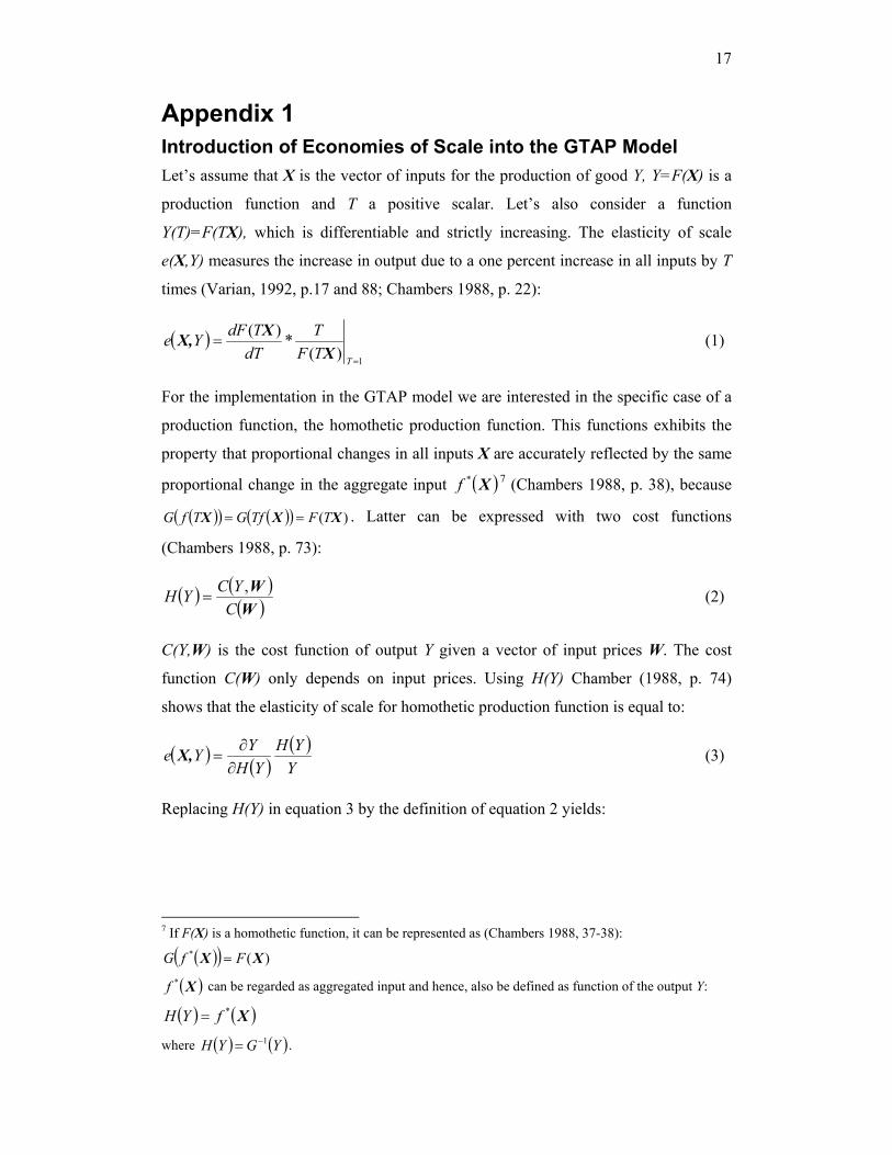
Appendix 1 Introduction of Economies of Scale into the GTAP Model Let’s assume that X is the vector of inputs for the production of good Y, Y=F(X) is a

production function and T a positive scalar. Let’s also consider a function

Y(T)=F(TX), which is differentiable and strictly increasing. The elasticity of scale

e(X,Y) measures the increase in output due to a one percent increase in all inputs by T

times (Varian, 1992, p.17 and 88; Chambers 1988, p. 22):

( )1)(

*)(

=

=TTF

TdTTdFYe

XXX, (1)

For the implementation in the GTAP model we are interested in the specific case of a

production function, the homothetic production function. This functions exhibits the

property that proportional changes in all inputs X are accurately reflected by the same

proportional change in the aggregate input ( )X*f 7 (Chambers 1988, p. 38), because

( )( ) ( )( ) )( XXX TFTfGTfG == . Latter can be expressed with two cost functions

(Chambers 1988, p. 73):

( ) ( )( )WW

CYCYH ,

= (2)

C(Y,W) is the cost function of output Y given a vector of input prices W. The cost

function C(W) only depends on input prices. Using H(Y) Chamber (1988, p. 74)

shows that the elasticity of scale for homothetic production function is equal to:

( ) ( )( )YYH

YHYYe

∂∂

=X, (3)

Replacing H(Y) in equation 3 by the definition of equation 2 yields:

7 If F(X) is a homothetic function, it can be represented as (Chambers 1988, 37-38):

( )( ) )(* XX FfG =

( )X*f can be regarded as aggregated input and hence, also be defined as function of the output Y:

( ) ( )X*fYH =

where ( ) ( )YGYH 1−= .

18

( )( )( )

( )( )WW

WW

X,CYYC

YCYC

Ye*

,,

1

∂

∂

= (4)

After some rearrangements we get:

( ) ( )( )

( )( )WW

WWX,

CYAC

YYC

CYe ,,

∂∂

=

AC(Y,W) is the average cost of the produced output Y. After a further simplification

the above equation becomes:

( ) ( )( )WWX,,,

YMCYACYe = (5)

MC(Y,W) is the marginal cost of the produced output. We introduce now equation 5 in

equation 3 and rearrange it:

( )( )

( )( )WW,,

YMCYAC

YdHYH

YdY

= (6)

We assume that ( ) ( )WW CYYC θ=, respectively ( ) θYYH = whereas 0 < θ < 1 (Francois

1998, p. 2). Accordingly, AC(Y,W)/ MC(Y,W) is constant8. Equation 6 can be

formulated by using percentage changes ^Y and

^H (Francois 1998, p.3):

^^H

MCACY = (7)

If e > 1 or equivalently AC > MC then output increase more than scale of input and

the technology exhibit increasing returns to scale. To show the scale effect, it is useful

to formulate equation 7 in the following way:

( )^^

H1SCALEY += (8)

Where

MCMCACSCALE −

= (9)

8 The relation AC/ MC is constant since: ( )

( )( ) θ1

YCYCY

MCAC

=

∂∂

=−

WW

θ

θ 1

19

describes the additional output growth when inputs increase.

To calculate SCALE, Francois (1998, p.3) employs the Cost Disadvantage Ratio

(CDR)9:

CDR1CDRSCALE−

= (10)

Since the GTAP standard model assumes no economics of scale, Francois (1988)

suggests to introduce them in the upper level nest (output nest) of the production tree

in which the Leontief production function is applied. Following Francois (1998, p.3),

we assume that the additional output change from the economies of scale is

accommodated by the parameter of the technical progress of the whole production of

sector i, that alter parameters of the Leontief production function in such a way that:

^^

iXaoallY += (11)

and therefore

^^^HXX ij == for all i and j (12)

Equation (11) can be then rearranged as:

iXH

aoall1Y ˆ^

^

+= (13)

which is in fact equation (8) in a case of the Leontief production function with

SCALE parameter equal to:

^H

aoallSCALE = (14)

To represent the input change in equation (14) we use the variable qva(i,r), which

indicates the quantity change of the factor bundle input in sector i of region r10 and

equation (14) in GTAP notation becomes:

),(*),(),( riqvariSCALEriaoall = (15)

9

ACMCACCDR −

=

10 Since GTAP is a multi regional model we have to add the index r for region.

20

Equation (15) has to be added to the GTAP standard model. Normally, aoall(i,r) is an

exogenous variable. Through the introduction of equation (15) aoall(i,r) becomes

endogenous, which indicates a change of the model closure.

Since we assume external economies of scale we can maintain the assumption of

perfect competition of the standard GTAP model (Krugman and Obstfeld, p.123).

21

CDR Coefficients and Output Changes Table 10: CDR Coefficients Sector CDR Rice 0 Grains 0 Fibers 0 rAGR 0 Food 0.055 Textiles 0.055 Wearing apparel

0.055

Leather products

0.055

Extract 0.075 LiMANF 0.085 CiMANF 0.085

Services

0.025 Bangladesh, Sri Lanka, rSAFTA, China, cAmerika, ROW 0.05 India, oAsia, CEEC, Turkey 0.105 hASIA, EU, USA, Canada

Source: Francois et al. (2002)

Table 11: Output Changes in Percent for the SAFTA Scenario (All Regions)

qo Bang

la-

desh

Indi

a

Sri L

anka

rSAF

TA

Chi

na

hASI

A

oASI

A

EU

CEE

C

Turk

ey

USA

Can

ada

cAM

ERIK

A

RO

W

Rice -0.3 -0.7 -5.3 0.1 -0.7 0.1 0.4 0.3 3.6 -2.1 1.2 0.7 0.1 0.3 Grains 1.5 -0.1 -0.2 -0.4 0.8 -11.3 -0.3 0.4 -2.2 -1.6 -1.9 0.3 0.2 -0.2 Fibers 5.9 -0.7 1.2 -0.3 9.8 1.2 0.2 -1.1 3.3 12.8 -1.5 -0.1 -6.5 -0.1 rAGR 0.8 -0.5 0.4 -0.1 -0.7 0.2 -0.2 0.2 -0.9 -1.5 0.6 -0.0 0.4 0.0 Food -0.3 -2.9 -1.9 -1.7 -1.4 0.4 -0.1 0.1 0.8 -1.2 0.2 0.1 0.3 -0.0 Textiles 0.3 8.7 14.3 8.6 11.4 2.7 4.1 -4.8 8.0 29.4 -7.6 -12.3 -12.8 -2.6 Wearing apparel -15.9 153.8 1.9 -7.8 40.1 -3.0 -0.8 -17.8 49.0 51.1 -22.2 -35.1 -35.4 -6.6 Leather products 29.7 -31.9 2.6 -9.7 -7.3 1.6 2.0 3.2 16.5 1.8 2.2 1.0 2.7 0.8 Extract 0.2 -3.9 -0.4 -0.8 -1.4 0.1 -0.0 -0.0 -3.0 -2.5 0.2 0.2 0.9 0.2 LiMANF 4.1 -4.6 -0.3 0.9 -2.2 -0.0 -0.1 0.4 -4.6 -5.1 0.2 0.4 1.4 0.2 CiMANF 4.6 -7.3 5.6 -1.8 -4.3 0.0 -0.4 0.6 -5.5 -2.0 0.8 1.0 6.6 0.5 Services -0.2 -0.4 -0.9 -0.3 -0.4 -0.0 -0.0 0.0 0.2 -0.2 0.1 0.2 0.1 0.0 Source: model simulations

22

Table 12: Output Changes in Percent for the WTO-EU Scenario (All Regions)

qo Bang

la-

desh

Indi

a

Sri L

anka

rSAF

TA

Chi

na

hASI

A

oASI

A

EU

CEE

C

Turk

ey

USA

Can

ada

cAM

ERIK

A

RO

W

Rice 0.8 1.0 7.5 1.2 -0.9 -3.7 0.5 -19.9 1.0 -6.8 6.3 6.0 -1.6 0.7 Grains 9.7 0.7 -8.0 -0.8 -1.9 -31.5 -1.8 -10.5 0.2 -1.0 -0.3 13.9 -0.8 0.6 Fibers -2.4 -0.5 -11.4 -0.0 12.5 11.5 -1.8 -0.8 -4.5 10.0 -1.0 5.7 -8.6 0.7 rAGR 2.4 0.7 0.1 1.6 -1.2 -3.3 -0.7 0.1 -1.8 -0.9 1.3 -0.7 1.1 -0.2 Food 12.1 2.9 4.1 9.6 -2.6 -1.6 0.3 -1.1 -0.1 -1.8 0.8 -1.3 0.8 0.6 Textiles -4.8 10.7 16.3 9.1 14.7 12.1 26.6 -6.6 1.1 23.6 -11.1 -19.3 -16.5 -5.3 Wearing apparel -18.8 199.0 23.4 4.7 60.1 -6.0 41.8 -23.6 19.2 40.0 -30.4 -50.2 -43.3 -9.2 Leather products 32.1 -40.4 -24.9 -27.7 -0.3 5.0 95.8 -5.1 4.6 -0.4 -9.8 -25.9 -7.1 -5.5 Extract 0.6 -6.8 -3.8 -2.3 -2.3 -0.7 -2.7 -0.0 -2.5 -2.2 0.4 0.7 0.8 0.3 LiMANF 1.7 -7.7 -8.0 -6.6 -4.5 1.3 -6.7 0.7 -3.0 -4.4 0.3 -0.1 1.8 -0.4 CiMANF -0.2 -12.7 -41.6 -6.8 -5.7 -0.0 -1.9 0.6 -2.4 -0.3 1.9 2.7 8.2 -0.3 Services -0.3 -0.6 -1.2 -0.5 -0.3 -0.0 -0.6 0.2 0.7 -0.1 -0.0 0.3 0.1 0.3 Source: model simulations

Table 13: Output Changes in Percent for the WTO-US Scenario (All Regions)

qo Bang

la-

desh

Indi

a

Sri L

anka

rSAF

TA

Chi

na

hASI

A

oASI

A

EU

CEE

C

Turk

ey

USA

Can

ada

cAM

ERIK

A

RO

W

Rice 0.3 -1.0 -2.4 0.1 -0.1 -16.9 1.2 -32.0 1.3 -8.9 53.1 10.2 0.2 3.6 Grains 10.9 -0.1 -10.8 0.2 4.5 -63.2 1.2 -23.9 2.1 0.5 -1.4 30.9 0.3 1.2 Fibers -0.7 -1.0 -3.9 0.5 10.9 23.4 -0.7 1.8 -4.0 9.5 -2.8 12.8 -9.0 -0.5 rAGR 2.2 -0.6 -1.5 -0.7 -1.6 -4.3 -1.2 -0.9 -2.1 0.4 2.7 -2.0 1.8 -0.2 Food 3.1 -3.9 -9.4 -4.8 -2.6 -1.7 1.5 -2.3 -2.3 -3.3 1.7 -3.3 1.5 1.6 Textiles -9.4 10.5 14.1 17.1 12.8 12.2 12.5 -5.5 2.1 23.9 -10.5 -17.8 -17.0 -5.8 Wearing apparel 0.8 202.7 47.6 30.4 55.0 -3.6 14.1 -21.5 23.9 44.7 -28.1 -47.4 -43.1 -10.1 Leather products 69.8 -33.5 -28.6 6.2 3.5 9.9 39.4 -2.1 3.4 0.8 -8.7 -20.2 -5.6 -5.2 Extract 0.3 -6.7 -5.2 -5.3 -2.2 -0.4 -1.1 -0.2 -2.5 -2.5 0.4 0.6 0.8 0.1 LiMANF 0.9 -8.2 -6.1 -19.7 -4.0 1.2 -4.1 1.0 -3.4 -4.7 -0.1 -0.3 1.5 -0.5 CiMANF -0.9 -9.5 -21.6 -10.2 -5.5 0.2 0.3 0.3 -1.3 -0.3 1.1 1.9 7.5 0.3 Svces -0.0 -0.1 -1.3 0.9 -0.4 0.0 -0.2 0.3 0.7 -0.3 0.0 0.3 0.0 0.2 Source: model simulations