Multilateral Trade Bargaining:A First Look at the

GATT Bargaining Records∗

Kyle Bagwell† Robert W. Staiger‡ Ali Yurukoglu§

Preliminary: February 2015

Abstract

This paper empirically examines recently declassified data from the GATT/WTO ontariff bargaining. We document eight stylized facts about these interconnected high-stakesinternational negotiations. We use detailed product-level offer and counteroffer data toexamine several questions about trade policy, including whether preferential tariffs were astumbling block towards liberalization, and whether the relaxation of bilateral reciprocityto multilateral reciprocity aided liberalization. We organize the empirical analysis arounda theoretical model of multi-party trade negotiations motivated by the terms-of-trade the-ory and respecting the institutional features of most-favored-nation status and reciprocity.

∗We thank the NSF (Grant SES-1326940) and SEED for financial support, and Sushan Demirjian, DiwakarDixit, Anwarul Hoda, Lee Ann Jackson, William Powers and Suja Rishikesh for very helpful discussions relatedto various aspects of this project. We are especially grateful to Ambassador Julio Lacarte Muró for patientlyanswering our many questions about the mechanics of the early GATT rounds. We also thank Jakub Kastl,Marzena Rostek and seminar participants at Berkeley, Dartmouth, Princeton and Stanford as well as participantsat the Dartmouth-SNU conference on International Trade Policy and Institutions for very helpful comments onan earlier draft. Patricia Abbott, Ayako Obashi, Woan Foong Wong and Junhui Zeng provided outstandingresearch assistance, as did Joanna Yeo, Zhufei Shi, and especially Elizabeth Stone on earlier phases of the dataprocessing portion of this project.†Department of Economics, Stanford University; and NBER.‡Department of Economics, Dartmouth College; and NBER.§Graduate School of Business, Stanford University and NBER

1. Introduction

The World Trade Organization (WTO) and its predecessor the General Agreement on Tariffs

and Trade (GATT)1 have presided over the largest and most sustained negotiated trade lib-

eralization in history. Yet challenges remain, as evidenced by the 13-year-long Doha Round

of multilateral trade negotiations now certain to fall far short of its initial aspirations. This

paper introduces and empirically analyzes detailed negotiation data, recently declassified by the

WTO, to understand the nature of tariffbargaining in the world trading system. Improving our

understanding of these negotiations is important for addressing the challenges facing modern

trade agreements. At the same time, analyzing these detailed offer data in high stakes interna-

tional negotiations contributes to economists’understanding of bargaining more generally.

GATT/WTO tariff negotiations display several notable features. First, these negotiations

are a form of barter, whereby governments accept commitments on their own import tariffs

in exchange for the reciprocal tariff commitments of their principal trading partners. Second,

for each round a specific bargaining protocol is adopted, with explicit rules for the timing of

events, the kinds of interactions expected and the exchange of information among participants.

And finally, though it is a multilateral institution, for the most part the GATT/WTO has

adopted a bilateral approach to multilateral tariff bargaining according to which reciprocal

negotiations occur on a voluntary basis between pairs of countries, with the results of these

bilateral negotiations then “multilateralized”to the full GATT/WTO membership by a non-

discrimination requirement that tariffs abide by the most-favored nation (MFN) principle.

Our empirical analysis has two major components, both of which focus on the US bilateral

negotiations at the Torquay (1950-1951) Round. We first describe the salient features of these

high stakes negotiations: Howmany tariff-cut offers are made?; How large are the offers?; Which

countries receive offers on which goods?; How do offers evolve over the course of negotiations?;

and so on. Then we ask a series of classic trade policy questions: Does the multilateralization of

trade bargaining aid liberalization?; Are preferential tariffs a building block or stumbling block

towards liberalization?; Are negotiating patterns consistent with the terms-of-trade theory?

With these two components we show how the new data present a major research opportunity

for economists interested in international trade policy, economic history, or bargaining theory.

1The GATT was created in 1947, and it sponsored a total of eight multilateral negotiating rounds through1994. With the conclusion of the eighth (Uruguay) round, the WTO came into existence on January 1, 1995,and it includes the GATT and a set of additional agreements that extend GATT principles to new areas.

1

To structure our empirical analysis, we establish a theoretical and institutional framework.

This framework adopts the perspective of the terms-of-trade theory of trade agreements (see

Bagwell and Staiger, 2010a, for a recent review of the central features of this theory). On top

of the basic theory, we layer the institutional features of reciprocity and MFN. Reciprocity

requires that equilibrium agreements increase export volume for a given country by the same

amount as the increase in its import volume. MFN requires that any concession granted in a

bilateral negotiation be extended to the other members of GATT.

With this framework established, we document a series of stylized facts about the negotia-

tions. We find that the numbers of back-and-forth offers and counter-offers in any bargain are

relatively small, and that the bargaining appears to have taken the form of essentially take-it-

or-leave-it offers on the intensive margin (the level of the tariff cut offered) and back-and-forth

offers and counter-offers on the extensive margin (which products are to be included in the

bargain). We document that countries make counter-proposals by adjusting the set of tariff

cuts they offer, but do not propose adjustments to what their bargaining partners have offered.

Substantial numbers of offers are made that were not requested by the country to which the

offer is extended, and some offers are made that were not requested by any country at all. There

is substantial two-way bargaining within narrow product categories, and significant numbers

of these two-way bargains occur within a single bilateral. The biggest supplying countries play

the dominant role in negotiations, but the role of smaller supplying countries can also be sig-

nificant. The set of requests a country entertains seems to conform with the principal supplier

rule, but when it comes to deciding which bargaining partners to make requests of on a given

product there appears to be a more narrow focus than principal supplier considerations would

dictate. And initial offers can sit dormant for long periods only to be finalized with a single

modification at the time that other bargains are concluded.

After establishing these stylized facts, we turn to analyzing the role of multilateralism in

the negotiations. While negotiations occurred bilaterally, the fact that they were occurring

simultaneously and in geographic proximity to each other allowed the possibility that some

negotiations might succeed by building on others. Put simply, if country A wants a concession

from country B, and country B from country C, and country C from country A, negotiation

outcomes that respect bilateral reciprocity would fail whereas bilateral negotiations which re-

spect only multilateral reciprocity can succeed. Indeed, writings from the time placed great

emphasis on the role of GATT in facilitating multilateral as opposed to bilateral reciprocity, as

2

illustrated by the following exert from an early GATT report:

Multilateral tariff bargaining, as devised at the London Session of the Preparatory

Committee in October 1946 and as worked out in practice at Geneva and Annecy, is

one of the most remarkable developments in economic relations between nations that has

occurred in our time. It has produced a technique whereby governments, in determining

the concessions they are prepared to offer, are able to take into account the indirect

benefits they may expect to gain as a result of simultaneous negotiations between other

countries, and whereby world tariffs may be scaled down within a remarkably short time.

(ICITO, 1949, p. 10)

We look for evidence that GATT played this role using the offer and counteroffer data from

Torquay, and we exploit a “natural experiment”: the breakdown of the US-UK bilateral midway

through the round. Specifically, we test whether, after this breakdown, the US was more likely

to extend offers on products to third parties when these products were involved in the failed

US-UK negotiation. We find that goods which the US was negotiating with the UK were more

likely to be revised into new US offers to other countries following the breakdown at the same

time that these other countries were withdrawing offers to the US, indicating that these other

countries had been counting on concessions from negotiations to which they were not party.

We close by modelling the decision to make an offer on a product, and the success of the

offer in becoming a finalized concession. We focus on US offers, and use a specification that

is suggested by our theoretical and institutional framework, modeling these outcomes at the

product level as functions of the exporter concentration of the product into the US, the extent to

which major exporters of the product to the US were members of a preferential tariff agreement

(PTA) with third countries, the extent to which the US had a reciprocal desire for tariff cuts

from the major exporters of the product into the US, the fraction of exports of the product

to the US that came from countries that were not present at Torquay, the degree of product

differentiation, a product-level measure of importer market power exerted by the US, whether

any country requested a tariff concession from the US on the product, and whether the US had

previously bound the product’s tariff.

From the specification of these offer and failure equations, we find that the US was more

likely to make offers, and these offers were more likely to succeed, when the US measure of

importer market power is higher. This finding supports the basic premise of the terms-of-trade

3

theory. Our findings regarding PTAs are more guarded: we find that the US was more likely

to make offers on products where a PTA member was a major supplier of that product to the

US market; but we also find that those offers were more likely to fail. On net, the first effect

outweighs the second, and so our findings lend support to the view that PTAs were building

blocks for US liberalization at Torquay. We do not find evidence in either our offer or failure

equation that the US faced a major free-rider problem associated with MFN, which is in line

with the predictions of the terms-of-trade theory when MFN is combined with reciprocity.

Our paper is related to several literatures. Recent papers in international trade have asked

whether there is empirical support for the terms-of-trade theory of trade agreements (e.g.,

Broda, Limao and Weinstein, 2008, Bagwell and Staiger, 2011, Ludema and Mayda, 2013,

Bown and Crowley, 2013), whether MFN creates a free-rider problem for trade negotiations (e.g.,

Ludema and Mayda, 2009, 2013 ), and whether PTAs create building blocks or stumbling blocks

for multilateral liberalization (e.g., Limao, 2006, Karacaovali and Limao, 2008, Estevadeordal,

Freund and Ornelas, 2008). And economic historians and political scientists have long debated

what made GATT special as an institution for promoting trade liberalization (e.g., Irwin, 1995,

and Gowa and Kim, 2005). Our paper provides evidence on each of these questions, but for

the first time from the perspective of actual tariff bargaining data.

In the context of the empirical bargaining literature, a handful of papers empirically examine

bilateral bargaining with not just outcome data, but detailed offer and counter-offer data. These

include Keniston (2013) and Larsen (2014). In these settings, bilateral negotiations do not affect

payoffs of parties not involved in the bargain. In parallel, there is an emergent literature in

industrial organization empirically examining bilateral bargaining with externalities using data

on only outcomes as in Crawford and Yurukoglu (2012). Our paper is unique in looking at

detailed offer and counter-offer data in a setting of bilateral bargaining with externalities.

The remainder of the paper proceeds as follows. In section 2 we present the basic theory

of trade negotiations that guides our empirical analysis of the GATT bargaining data. We

describe the GATT bargaining protocols in section 3, and in section 4 we discuss the broad

features of the GATT bargaining data. In section 5 we present summary statistics relating

to the US Torquay bilaterals and describe stylized facts about multilateral tariff bargaining

that are suggested by these bargaining records. In sections 6 and 7 we draw on our theoretical

framework and present our empirical analysis of multilateralism in the negotiations and the

determinants of offers and bargaining failure. Section 8 concludes.

4

2. The Theory of Trade Negotiations

In this section, we present the theory of trade negotiations that guides our empirical analysis.

2.1. The Trade Negotiation Problem

We begin by reviewing the textbook two-good general-equilibrium model of trade between

two countries, defining a general family of government preferences, and using the resulting

framework to identify the problem that a trade agreement can solve. For this purpose we

paraphrase the treatment in Bagwell and Staiger (2010a), and refer readers there for details.

The Model Two countries, domestic (no *) and foreign (*), trade two goods which are

normal in consumption and produced in perfectly competitive markets under conditions of

increasing opportunity costs. We let x (y) denote the natural import good of the domestic

(foreign) country. The local relative price facing domestic (foreign) producers and consumers is

defined as p ≡ px/py (p∗ ≡ p∗x/p∗y). Tariffs are non-prohibitive, and we represent the domestic

(foreign) ad valorem import tariff as t (t∗). Letting τ ≡ (1 + t) and τ ∗ ≡ (1 + t∗), we then have

that p = τpw ≡ p(τ , pw) and p∗ = pw/τ ∗ ≡ p∗(τ ∗, pw), where pw ≡ p∗x/py is the “world”(i.e.,

untaxed) relative price. The foreign terms of trade is given by pw, and the domestic terms of

trade is 1/pw. We interpret τ > 1 as an import tax and similarly for τ ∗.

In each country, production levels for x and y are determined by the local relative price:

Qi = Qi(p) and Q∗i = Q∗i (p∗) for i = {x, y}. Consumption is also influenced by the local

relative price, which defines the trade-off faced by consumers and determines the level and

distribution of factor income. Consumption depends as well on tariff revenue R (R∗), which

is measured in units of the local export good at local prices and is distributed lump-sum to

domestic (foreign) consumers. Domestic and foreign consumption thus may be represented as

Di = Di(p,R) and D∗i = D∗

i (p∗, R∗) for i = {x, y}. But tariff revenue is implicitly defined by

R = [Dx(p,R)−Qx(p)][p−pw] or R = R(p, pw) for the domestic country, and similarly we have

that R∗ = [D∗y(p

∗, R∗) − Q∗y(p∗)][1/p∗ − 1/pw] or R∗ = R∗(p∗, pw) for the foreign country; and

each country’s tariff revenue increases with its terms of trade, given our assumption of normal

goods. Hence, we may express national consumption as a function of local and world prices:

Ci(p, pw) ≡ Di(p,R(p, pw)) and C∗i (p∗, pw) ≡ D∗

i (p∗, R∗(p∗, pw)) for i = {x, y}.

Imports of x and exports of y for the domestic country are respectively defined byM(p, pw) ≡

5

Cx(p, pw)−Qx(p) and E(p, pw) ≡ Qy(p)−Cy(p, pw). Likewise, for the foreign country, we have

M∗(p∗, pw) and E∗(p∗, pw), respectively. For any prices, domestic and foreign budget constraints

are represented by the trade-balance equations:

pwM(p, pw) = E(p, pw), and M∗(p∗, pw) = pwE∗(p∗, pw). (2.1)

The equilibrium world price, p̃w(τ , τ ∗), is determined by market clearing for good y:

E(p(τ , p̃w), p̃w) = M∗(p∗(τ ∗, p̃w), p̃w), (2.2)

where we make explicit in (2.2) the functional dependencies for local prices. Market clearing

for good x is then guaranteed by (2.1) and (2.2).

We assume dp/dτ > 0 > dp∗/dτ ∗ and ∂p̃w/∂τ < 0 < ∂p̃w/∂τ ∗, thereby ruling out the

Metzler and Lerner paradoxes, and with the final two inequalities indicating that each country

is “large”(i.e., each country can improve its terms of trade by increasing its tariff).

Government Preferences The traditional approach to representing government preferences

is to impose the assumption that governments maximize national income; by contrast, in the

political-economy approach, governments are motivated by distributional concerns. Here, we

follow Bagwell and Staiger (1999, 2002) and adopt a general approach to modeling government

preferences, representing the objectives of the domestic and foreign governments with the gen-

eral functions W (p, p̃w) and W ∗(p∗, p̃w), respectively. We thus represent welfare in terms of

the prices that the tariffs induce rather than directly in terms of the tariffs themselves. This

approach enables us to disentangle the separate roles played by the terms-of-trade externality

and political motivations in explaining the purpose of a trade agreement.

We place no restrictions on government preferences over local prices: as local prices deter-

mine the level and distribution of factor incomes, we therefore accommodate a wide range of

political motivations. We assume only that, holding its local price fixed, each government is

pleased when its terms of trade improve:

Wp̃w < 0 and W ∗p̃w > 0. (2.3)

The meaning of (2.3) in terms of the underlying tariff changes is that a government values the

international income transfer that is implied by an increase in its own tariff and a decrease in

the tariff of its trading partner that together leave its local price unaltered. As Bagwell and

Staiger (1999, 2002) discuss, governments maximize welfare functions of this form in both the

traditional approach and in the leading political-economy approaches to trade policy.

6

Unilateral Policies To analyze optimal unilateral (non-cooperative) policies, we suppose

that each government sets its tariff policy to maximize its welfare, for any given tariff choice of

its trading partner. The associated tariff reaction curves are defined implicitly by

Wp + λWp̃w = 0, and (2.4)

W ∗p∗ + λ∗W ∗

p̃w = 0, (2.5)

where λ ≡ [∂p̃w/∂τ ]/[dp/dτ ] < 0 and λ∗ ≡ [∂p̃w/∂τ ∗]/[dp∗/dτ ∗] < 0. As these expressions

highlight, the best-response tariff of each government strikes a balance between the effects on

its welfare of the local- and world-price movements induced by its tariff choice.

The welfare implications of the local-price movement in the first term of (2.4) are domestic

in nature: they reflect the trade-off for the domestic government between the costs of the

induced economic distortions and the benefits of any induced political support. By contrast, the

welfare implications of the world-price movement in the second term of (2.4) are international

in nature: they reflect the benefits to the domestic government of shifting some of the costs of

its policy choice onto the foreign government. Cost shifting occurs, since any improvement in

the domestic country’s terms of trade is a deterioration in the foreign country’s terms of trade.

We may similarly interpret (2.5) for the foreign government.

In a Nash equilibrium, both governments are on their reaction curves, and a Nash equilib-

rium tariff pair (τN , τ ∗N) thus satisfies (2.4) and (2.5). We take this equilibrium to represent

the trade-policy decisions that governments would make if there were no trade agreement.

Trade Agreement Governments value a trade agreement if it leads to changes in trade

policies that generate Pareto improvements for governments relative to their welfare in the

Nash equilibrium. Thus, a trade agreement is potentially valuable if and only if the Nash

equilibrium is ineffi cient, when effi ciency is measured relative to government preferences.

Three observations can be stated.2 First, Nash tariffs are indeed ineffi cient. Second, both

governments can gain relative to Nash only if each agrees to set its tariff below its Nash level.

The first observation means that a mutually beneficial trade agreement is possible, while the

second observation implies that reciprocal trade liberalization is necessary for mutual gains.

Intuitively, when a government contemplates an increase in its unilateral tariff, it foresees an

improvement in its terms of trade; thus, it is in part motivated by the prospect of shifting some

2Formal proofs of these observations can be found in Bagwell and Staiger (1999, 2002).

7

of the costs of the tariff hike onto its trading partner. The incentive to shift costs naturally

leads governments to set tariffs that are higher than is effi cient.

To see if the terms-of-trade externality is the only reason for the ineffi ciency of Nash tariffs,

consider a hypothetical world in which governments are not motivated by the terms-of-trade

implications of their unilateral trade-policy choices, that is, a hypothetical non-cooperative set-

ting in which Wp̃w ≡ 0 and W ∗p̃w ≡ 0. Next define the “domestic politically optimal reaction

curve”by Wp = 0, the “foreign politically optimal reaction curve”by W ∗p∗ = 0, and the politi-

cally optimal tariffs as any tariff pair (τPO, τ ∗PO) that satisfies Wp = 0 and W ∗p∗ = 0. The third

observation is that politically optimal tariffs are effi cient (when evaluated with actual govern-

ment preferences): the terms-of-trade externality is the sole rationale for a trade agreement in

this (“terms-of-trade theory”) modeling framework.

The politically optimal tariffs are not the only effi cient tariffs. In the special case where

governments maximize national welfare, effi cient tariffs satisfy τ = 1/τ ∗ (as Mayer, 1981 shows)

and politically optimal tariffs correspond to reciprocal free trade (i.e., τ = τ ∗ = 1), a point on

the Mayer locus. A trade agreement enables governments to move from the ineffi cient Nash

tariffs to some point on the contract curve, where the contract curve is that portion of the

effi ciency frontier on which neither government receives below-Nash welfare. The politically

optimal tariffs lie on the contract curve, provided that the countries are not too asymmetric.

2.2. Reciprocity and MFN: Implications for the GATT bargaining data

We next consider the implications of the key GATT/WTO institutional features of reciprocity

and MFN for tariff bargaining and thus the GATT bargaining data. We note at the outset

that there are (at least) two complementary approaches to analyzing the GATT bargaining

data. A first approach emphasizes strict adherence to reciprocity and MFN. The benefit of this

approach is that it can afford a powerful simplification to the GATT bargaining problem and

thereby provide structure to the analysis of the bargaining data. In this paper we emphasize

this approach. A second approach confronts the complications that arise when adherence

to reciprocity and/or MFN is not strict. This approach uses models of bilateral bargaining

with externalities, informed by other institutional features of the GATT bargaining setting, to

analyze the bargaining data. We leave this second approach to future work.

We show below that the GATT/WTO pillars of reciprocity and MFN can dramatically

simplify the tariff bargaining problem. First, building on the two-country model in section 2.1,

8

we explain that strict adherence to reciprocity simplifies strategic considerations resulting in

a dominant bargaining strategy. Second, in a multi-country version of the model, we confirm

as well that strict adherence to reciprocity and MFN neutralizes third-party externalities. But

there is also a potential cost: if GATT bargaining partners are asymmetric in a sense described

below, then strict adherence to reciprocity and MFN also prevents governments from reaching

the effi ciency frontier. Finally, to provide further structure for our empirical analysis, we also

examine the relationship between bilateral and multilateral reciprocity when MFN is satisfied.

Reciprocity We start with a review of the basic properties of reciprocity. For this purpose

we again paraphrase the treatment in Bagwell and Staiger (2010a), and refer readers there

for details. The GATT/WTO principle of reciprocity refers to the ideal of mutual changes

in trade policy which bring about changes in the volume of each country’s imports that are

equal in magnitude to the changes in the volume of its exports. The notion of reciprocity

arises in two places in the GATT/WTO. First, as we discuss in section 3, governments seek

a “balance of concessions” as a norm of negotiations, so that there is a rough equivalence

between the market access value of the tariff cuts offered by one government and the concessions

won from its trading partners. Second, when a government seeks to renegotiate, modify or

withdraw a previous concession as an original action, GATT Article XXVIII permits affected

trading partners to withdraw “substantially equivalent concessions,”and thereby to retaliate

in a reciprocal manner.

Continuing with the two-country model developed in section 2.1, we now state a formal

definition of reciprocity. Suppose that, beginning from an initial pair of tariffs, (τ 0, τ ∗0), a tariff

negotiation results in a change to a new pair of tariffs, (τ 1, τ ∗1). Denoting the initial world and

domestic local prices as p̃w0 ≡ p̃w(τ 0, τ ∗0) and p0 ≡ p(τ 0, p̃w0), and the new world and domestic

local prices as p̃w1 ≡ p̃w(τ 1, τ ∗1) and p1 ≡ p(τ 1, p̃w1), we say that the tariff changes conform to

the principle of reciprocity provided that

p̃w0[M(p1, p̃w1)−M(p0, p̃w0)] = [E(p1, p̃w1)− E(p0, p̃w0)], (2.6)

where changes in trade volumes are valued at the existing world price. We next use the domestic

balanced trade condition in (2.1) to establish that (2.6) may be rewritten as

[p̃w1 − p̃w0]M(p1, p̃w1) = 0. (2.7)

9

According to (2.7), reciprocity can be given a simple and striking characterization: mutual

changes in trade policy conform to the principle of reciprocity if and only if they leave the world

price unchanged. With this characterization in hand, we next consider how strict adherence to

reciprocity simplifies the complexity of the bargaining problem.

We examine an illustrative model. Let us take the pre-negotiation tariff pair as exogenous,

with the Nash tariffs being the natural candidate. The initial tariff pair fixes a particular

iso-world-price line, where as we illustrate below any such line is upward sloping in a graph

with tariffs on the axes. Following Bagwell and Staiger (1999), governments simultaneously

make tariff proposals, where any such proposal conforms to reciprocity and thus specifies a

tariff pair (τ , τ ∗) that lies along the fixed iso-world-price line. If the proposals agree, then

the common proposal is implemented; otherwise, the proposal with the higher tariff pair (i.e.,

the lowest trade volume) is implemented. This model clearly captures the reciprocal nature of

tariff liberalization negotiations in GATT; in addition, the structure of the game captures in

a short-hand way the potential for renegotiation under GATT Article XXVIII, since neither

government can be forced to import a volume greater than implied by its proposal.3

As established by Bagwell and Staiger (1999), strict adherence to reciprocity ensures that

it is a dominant strategy for each government to propose the tariff pair that if implemented

would deliver its preferred trade volume along the given iso-world-price line. Indeed, once the

iso-world-price line is fixed, this conclusion holds whether or not a government has private

information about its preferred local price. In this sense, strict adherence to reciprocity can

induce governments to truthfully reveal their politically optimal reaction curves. The key

features of the argument are illustrated in Figure 1 (which is an adaptation of Figure 4 in

Bagwell and Staiger, 1999).4

In the symmetric case, defined as when the Nash trade war leaves countries facing the same

terms of trade as would prevail at their politically optimal tariffs, strict adherence to reciprocity

leads to an effi cient outcome. To develop this point, we refer to Figure 1, which depicts τ on

3Under GATT Article XXVIII, if a negotiated tariff pair induces more trade volume than one governmentdesires given the world price, then that government could raise its tariff, knowing that the other governmentwould respond in reciprocal fashion. Our model captures this possibility in a short-hand way, by assuming thatthe proposal with the highest tariff pair is ultimately implemented. For more on the trade-effects interpretationof reciprocity in GATT/WTO practice in line with our discussion above, see Hoda (2001) and the Appellate BodyOpinion in WTO (2004). Limao (2006, 2007) and Karacaovali and Limao (2008) provide empirical evidencethat actual tariff bargaining outcomes in the GATT/WTO conform to a reciprocity norm.

4As we later discuss, with some additional structure this property implies that a researcher could invert tariffoffers to estimate government preferences.

10

w

PO

w

N pCp )(

W*

W

PO

E

E

W

B

B'

)(Bpw

N

)(Apw

N

W*

Wp*

* 0

Wp 0

A

A'

*

)(AN

)(CN

)(BN

Figure 1: Reciprocity and Politcally Optimal Reaction Curves

the vertical axis and τ ∗ on the horizontal axis. The symmetric case is illustrated by the Nash

point labeled N(C), which lies on the same iso-world-price locus as does the politically optimal

point, which is labeled PO and lies below N(C). In Figure 1 we label as pwN(C) = pwPO the

iso-world-price locus passing through both N(C) and PO. As reciprocity fixes the world price,

the two governments bargain along the iso-world-price locus pwN(C) = pwPO. The only dimension

on which the governments negotiate is the volume of trade to be exchanged at the fixed world

price (and trade volume is increasing as we move downward along the locus pwN(C) = pwPO).

At this fixed world price, the domestic government’s desired trade volume is determined where

its politically optimal reaction curve (labeled as Wp = 0) intersects the iso-world-price locus

pwN(C) = pwPO; and similarly the foreign government’s desired trade volume is determined where

its politically optimal reaction curve (labeled as W ∗p∗ = 0) intersects the iso-world-price locus

pwN(C) = pwPO. In the symmetric case, these two points of intersection correspond to the single

point which defines the political optimum (the point PO). Hence, according to Figure 1, the

governments would agree on the desired volume of trade. Since it is a dominant strategy for

each government in our game to propose the tariff pair that delivers its desired trade volume

(i.e., to truthfully reveal its politically optimal reaction curve), it follows that the outcome

of the bargaining game is the politically optimal tariff pair. Thus, in the symmetric case,

11

strict adherence to reciprocity ensures that the bargaining outcome yields an effi cient outcome

corresponding to the political optimum.

Now consider an asymmetric environment. Let us begin with point N(A). As in the symmet-

ric case above, the fact that reciprocity fixes the world price implies that the two governments

bargain along the iso-world-price locus passing through N(A), which we label pwN(A). At this

fixed world price, the domestic government’s desired trade volume is determined where its po-

litically optimal reaction curveWp = 0 intersects the iso-world-price locus pwN(A); and similarly

the foreign government’s desired trade volume is determined where its politically optimal re-

action curve W ∗p∗ = 0 intersects the iso-world-price locus pwN(A). But the two governments no

longer agree on the desired volume of trade; in particular, the foreign government’s desired

trade volume (labeled as A′) is less than the desired trade volume of the domestic government

(not labeled). In practice, this is where Article XXVIII comes in: any bargain that leaves

the governments on a point along the iso-world-price locus pwN(A) and which is below A′will

be renegotiated at the request of the foreign government up to the point A′. In terms of our

game, it is a dominant strategy for each government to propose the tariff pair that delivers its

desired trade volume (i.e., to truthfully reveal its politically optimal reaction curve), and so

the outcome of the bargaining process is the point A′. If GATT bargaining partners are asym-

metric in the sense that we have described above, then the strict adherence to reciprocity that

is necessary for this result will itself prevent governments from reaching the full information

effi ciency frontier (labeled EE in Figure 1).5

Reciprocity with MFN We next consider MFN, and describe how reciprocity and MFN

together can eliminate bargaining externalities across bargaining pairs, thereby converting a

potentially complex multilateral bargaining problem into a comparatively straightforward set

of bilateral bargains. To develop this point, we extend the framework of section 2.1 to a world

of three countries. For this purpose we once again paraphrase the treatment in Bagwell and

Staiger (2010a), and refer readers there for details.

5We have developed these arguments allowing for the possibility that governments have private informationover their political preferences, but we conjecture that the same arguments apply if instead the private infor-mation that governments possess concerns their levels of impatience or threat points. Throughout, we assumethat governments are suffi ciently patient that the negotiated tariffs satisfy self-enforcement constraints, and ourconjecture is understood in this context. Finally, governments might also have private information about theform of import demand and/or export supply functions, in which case they might not agree as to the tariff pairsthat satisfy the principle of reciprocity. We leave consideration of this possibility for future work.

12

The domestic country now exports good y to two foreign countries, denoted by the su-

perscripts ‘∗1’and ‘∗2,’and imports good x from each of these countries (who do not trade

with each other). Each foreign country can impose a tariff on its imports of good y from the

domestic country (we denote the tariff of foreign-country i by τ ∗i), while the domestic country

can set tariffs on its imports of good x from the two foreign countries. If the domestic country

applies the tariff τ 1 to imports from foreign-country 1 and the discriminatory tariff τ 2 6= τ 1 to

imports from foreign-country 2, then separate world prices pw1 and pw2 apply to its trade with

foreign-countries 1 and 2 respectively. This follows because there can only be one local price

in the domestic economy, and the pricing relationships p = τ 1pw1 and p = τ 2pw2 then imply

pw1 6= pw2 whenever τ 1 6= τ 2.

The MFN rule imposes a very simple requirement: the domestic country must apply a

common tariff level τ 1 = τ 2 ≡ τ to the imports of x, regardless of whether these imports

originate from foreign-country 1 or 2. An important implication of the MFN rule is then that

a single equilibrium world price, p̃w(τ , τ ∗1, τ ∗2), must prevail; consequently, we may continue

to express government preferences with the simple representation W (p, p̃w), W ∗1(p∗1, p̃w) and

W ∗2(p∗2, p̃w), the same representation that we used in the 2-country setting.

In a multilateral world, the MFN principle ensures that the international externality at the

root of the problem to be solved by a trade agreement continues to exhibit the same structure

as in the simpler 2-country setting. This suggests that, in the company of MFN, the affi nity

between reciprocity and truth telling described above might extend to a multilateral setting.

We can show that this is indeed the case.

In addition, MFN and reciprocity together eliminate third-country spillovers from bilateral

tariff bargaining. To see why, consider the case where foreign-country 2 is not involved in the

negotiations and keeps its tariff unaltered. In the presence of MFN, the domestic government

and the government of foreign-country 1 can still negotiate a reciprocal reduction in their tariffs

τ and τ ∗1 which leaves the terms of trade p̃w(τ , τ ∗1, τ ∗2) unaltered but reduces p while raising

p∗1, and which therefore provides these two countries with greater trade volume. But recall now

that in foreign-country 2 we have the relationship p∗2 = pw/τ ∗2. It follows that, with τ ∗2 held

fixed, if the negotiation between the domestic country and foreign-country 1 abides by MFN

(so that a single equilibrium world price p̃w prevails) and reciprocity (so that p̃w is unaltered)

then p∗2 and therefore W ∗2(p∗2, p̃w) and foreign-country 2’s trade volume are unaltered by

these negotiations as well. In abiding by the principles of MFN and reciprocity, the domestic

13

government and the government of foreign-country 1 have thus engineered a bilateral tariff

bargain without third-country spillovers.6

In this general manner, reciprocity and MFN together can eliminate bargaining externalities

across bargaining pairs, while at the same time inducing truth-telling on the part of govern-

ments, thereby converting a potentially complex multilateral bargaining problem with private

information into a comparatively straightforward set of full-information bilateral bargains. Still,

as we have pointed out, if GATT bargaining partners are asymmetric, then the strict adherence

to reciprocity and MFN that is necessary for these results will itself prevent governments from

reaching the full information effi ciency frontier.

Multilateral Reciprocity The preceding discussion suggests a pragmatic solution for gov-

ernments to what might otherwise be an insurmountably complicated bargaining problem:

endeavor to set up the GATT multilateral bargaining problem as a collection of simultaneous

bilateral bargains that adhere strictly to the twin pillars of reciprocity and MFN.7 To provide

further structure for our empirical analysis, we now illustrate and examine the distinction be-

tween bilateral and multilateral reciprocity. As we describe further in section 6, this distinction

was emphasized in GATT writings at the time of the early rounds and will play an impor-

tant role in our empirical analysis. We argue that if a country’s tariffs satisfy MFN and if in

addition the bargaining outcomes lead to changes in the country’s trade volumes that satisfy

strict multilateral —but not necessarily bilateral —reciprocity, then (i) it is a dominant strategy

for the country to truthfully reveal its (effi cient-under-symmetry) politically-optimal-reaction-

curve tariffs in its initial offers, and (ii) the free rider problem should not arise and bargaining

6These and related points are developed in Bagwell and Staiger (2005, 2010b). An interesting question relatesto the role of the principal supplier rule in GATT/WTO bargaining if reciprocity and MFN induce the featureswe emphasize above. Our conjecture is that the principal supplier rule might still play two important rolesin this environment: first, where strict reciprocity is not feasible —because for example the dynamic effects oftariff liberalization make it diffi cult to achieve reciprocity in the short run even for tariff cuts that do achievereciprocity in the long run —and hence some spillovers become inevitable, arranging bargains in accordancewith the principal-supplier rule is a natural technique for minimizing third-party spillovers; and second, evenif all third-party spillovers were eliminated by a strict adherence to MFN and reciprocity, countries on the“long”side of the market for tariff cuts and who therefore face the prospect of being rationed in their abilityto find enough willing bargaining partners might naturally employ the principal supplier rule to prioritize theirbargaining efforts. In any case we view the development of a compelling answer to this question as an importanttask for future research.

7We have described these results in a simple 2-good model, and it remains to demonstrate that they extendto a many-good setting of the kind that would more accurately describe the GATT bargaining environment.We believe that the key features can be extended to such environments along the lines of Bagwell and Staiger(2002, Appendix B), but this extension remains an important task for future research.

14

externalities should not cause any problems for bargaining.

1

1

*1

*2

*3

y

x

x

x

1*

2*

3*

Figure 2: Multilateral Reciprocity

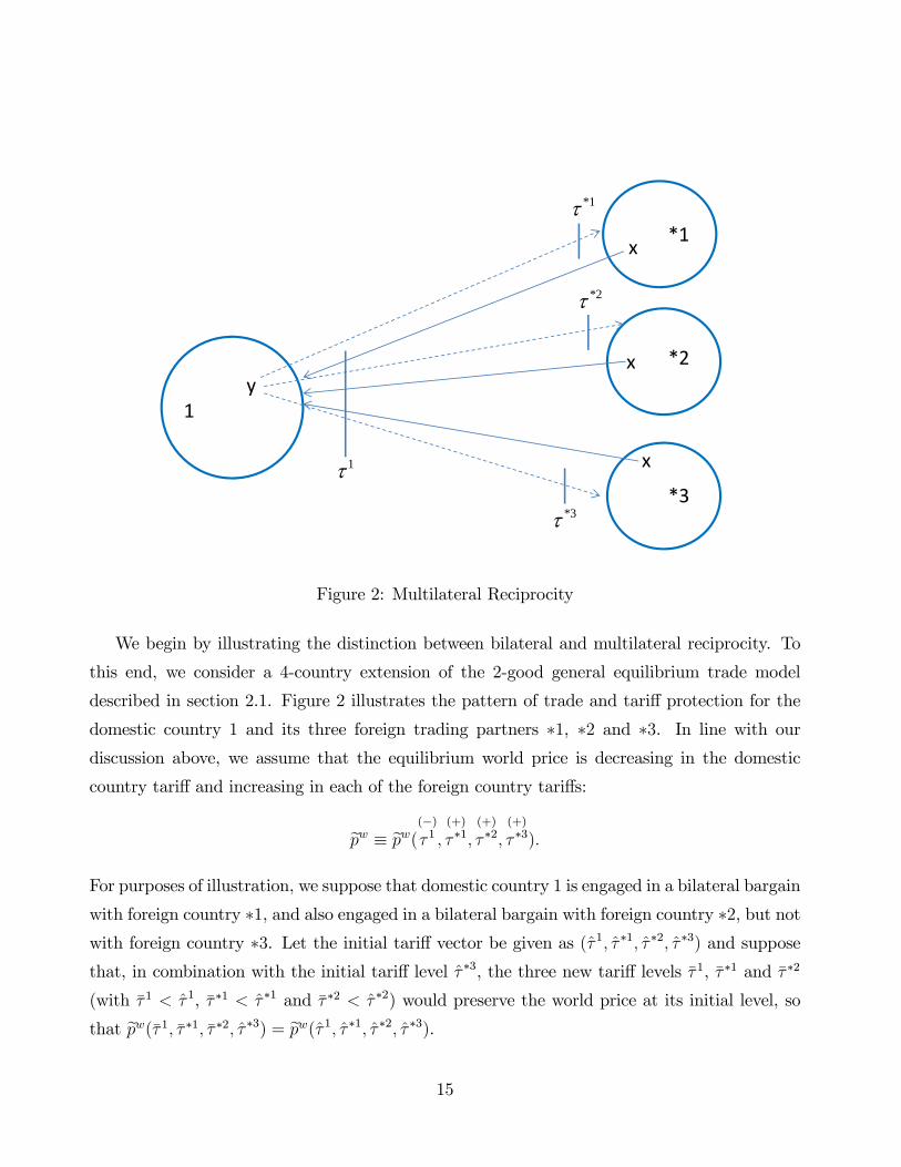
We begin by illustrating the distinction between bilateral and multilateral reciprocity. To

this end, we consider a 4-country extension of the 2-good general equilibrium trade model

described in section 2.1. Figure 2 illustrates the pattern of trade and tariff protection for the

domestic country 1 and its three foreign trading partners ∗1, ∗2 and ∗3. In line with ourdiscussion above, we assume that the equilibrium world price is decreasing in the domestic

country tariff and increasing in each of the foreign country tariffs:

p̃w ≡ p̃w((−)τ 1 ,

(+)

τ ∗1,(+)

τ ∗2,(+)

τ ∗3).

For purposes of illustration, we suppose that domestic country 1 is engaged in a bilateral bargain

with foreign country ∗1, and also engaged in a bilateral bargain with foreign country ∗2, but notwith foreign country ∗3. Let the initial tariff vector be given as (τ̂ 1, τ̂ ∗1, τ̂ ∗2, τ̂ ∗3) and suppose

that, in combination with the initial tariff level τ̂ ∗3, the three new tariff levels τ̄ 1, τ̄ ∗1 and τ̄ ∗2

(with τ̄ 1 < τ̂ 1, τ̄ ∗1 < τ̂ ∗1 and τ̄ ∗2 < τ̂ ∗2) would preserve the world price at its initial level, so

that p̃w(τ̄ 1, τ̄ ∗1, τ̄ ∗2, τ̂ ∗3) = p̃w(τ̂ 1, τ̂ ∗1, τ̂ ∗2, τ̂ ∗3).

15

We first illustrate a path from the initial to new tariffs that is characterized by bilateral

reciprocity between domestic country 1 and each of its two bargaining partners. Suppose the

domestic country starts with foreign country ∗1 and negotiates a reciprocal deal, in which thedomestic country lowers its tariff from τ̂ 1 to τ̃ 1 in exchange for a reciprocal reduction in the tariff

of foreign country ∗1 from τ̂ ∗1 to τ̄ ∗1, where the exchange preserves the level of p̃w. The domestic

country could then turn to foreign country ∗2 and negotiate an additional reciprocal deal, inwhich the domestic country agrees to a further lowering of its tariff from τ̃ 1 to τ̄ 1 in exchange

for a reciprocal reduction in the tariff of foreign country ∗2 from τ̂ ∗2 to τ̄ ∗2, again preserving the

level of p̃w. Each of the just-described bilaterals satisfies reciprocity (and each therefore leaves

the level of p̃w unchanged), and hence the bargain described conforms to bilateral reciprocity,

in the sense that the bilateral between the domestic country and foreign country ∗i involvesa reciprocal exchange of tariff cuts between the domestic country and foreign country ∗i, fori = 1, 2.8 Notice further that, since the bilateral negotiations leave the world price unaltered,

they do not affect foreign country ∗3, and thus do not give rise to a free-rider problem.We next consider an alternative path from the initial to new tariffs in which bilateral reci-

procity fails but multilateral reciprocity holds. In its bilateral with foreign country ∗1, supposethat the domestic country agrees to lower its tariff from τ̂ 1 to τ̄ 1 in exchange for a reduction

in the tariff of foreign country ∗1 from τ̂ ∗1 to τ̄ ∗1. The tariff changes agreed to in this bilateral

would by themselves result in a rise in the level of p̃w, as at the existing world price foreign

country ∗1 would experience a smaller increase in the volume of its exports than the increase inthe volume of its imports: these tariff changes are not bilaterally reciprocal. In its bilateral with

foreign country ∗2, suppose that the domestic country offers no further tariff cut but foreigncountry ∗2 agrees to lower its tariff from τ̂ ∗2 to τ̄ ∗2. The tariff changes agreed to in this bilateral

would by themselves result in a drop in the level of p̃w, as at the existing world price foreign

country ∗2 would experience a greater increase in the volume of its exports than the increasein the volume of its imports: these tariff changes are not bilaterally reciprocal either. Nev-

ertheless, taken together these two bilaterals satisfy multilateral reciprocity, as in combination

they do leave the world price unaltered; that is, both foreign country ∗1 and foreign country∗2 experience an equal increase in the volume of their exports and imports once each takesaccount of the indirect trade effects associated with the tariff changes negotiated in the other

8Indeed, the procedure we describe here corresponds to the so-called “split concession” procedure oftenutilized by the US in its sequential bilateral tariff bargains under the Reciprocal Trade Agreements Act thatpredated GATT (see Beckett, 1941, p. 23).

16

bilateral. Further, with the world price unaltered by the combination of bilaterals, a free-rider

problem does not arise, as foreign country ∗3 is again unaffected by the bilaterals.In our Online Supplementary Notes, we examine our dominant-strategy arguments in the

multi-country setting. Specifically, we assume that bilateral negotiations must satisfy MFN and

multilateral reciprocity, and develop one formalization of our dominant-strategy arguments for

a simple 3-country model (with one domestic country and two foreign countries). We define a

game in which the three countries take as given the initial tariff vector and the accompanying

world price, and then make simultaneous tariff proposals. A strategy for each country is a

proposal concerning its own tariff and that of its trading partner(s), where a proposal must

satisfy MFN and multilateral reciprocity (i.e., if accepted, the proposed tariffs would maintain

the initial world price). Since the foreign countries do not trade with one another, a proposal

from a foreign country leaves the tariff of the other foreign country at its initial value. As in the

2-country model above, each country’s proposal is associated with an “implied import volume”

for itself. We then construct a simple mechanism that takes the three proposals and assigns

a vector of tariffs. The domestic country’s proposal is assigned if the proposals agree.9 If the

proposals do not agree, we require that the constructed mechanism assigns a vector of tariffs

that maximizes the value of trade volume subject to maintaining the initial world price and not

forcing any country to import a volume in excess of its implied import volume.10

For the constructed mechanism, if countries use dominant strategies, we show that each

country’s proposal must specify a tariff for itself that delivers its preferred trade volume, given

the initial world price. As our 4-country illustration above suggests, a novel feature of the

multi-country setting is that the domestic country now has a set of dominant strategies. This

set is defined by proposals under which the domestic country proposes for itself the tariff that

9Agreement is defined to mean that, for any foreign country ∗i, the domestic country and foreign country∗i make the same proposal as regards foreign country ∗i’s tariff while foreign country ∗i is indifferent betweenits own proposal and the domestic-country proposal as regards the tariffs for the domestic country and foreigncountry ∗j, j 6= i.10This requirement delivers a unique tariff vector assignment when the value of the domestic country’s implied

import volume weakly exceeds the aggregate value of the foreign countries’ implied import volumes. If thedomestic country is on the “short”side, rationing occurs, and our requirement does not result in a unique tariffvector assignment. For this case, we construct the mechanism so that it randomly selects one foreign country tohave first priority. The constructed mechanism assigns tariffs such that the prioritized foreign country importsa volume equal to the minimum of its implied import volume and the value of the domestic country’s impliedimport volume, while the other foreign country imports a volume equal to the difference between the value ofthe domestic country’s implied import volume and the prioritized foreign country’s implied import volume (ifthat difference is positive). Similar results would obtain under other prioritization rules, provided that priorityis not influenced by foreign proposals (conditional on being in the case where the domestic country is short).

17

delivers its preferred trade volume given the world price and proposes for the foreign countries

any tariffs that when combined with the domestic tariffmaintain the world price and thus ensure

multilateral reciprocity. In this sense, it is again a dominant strategy for the domestic country

(and as before for the foreign countries as well) to truthfully reveal its politically-optimal-

reaction-curve tariffs in its initial proposal. We emphasize, though, that the set of dominant

strategies for the domestic country allows that its proposed tariff for itself may violate bilateral

reciprocity when paired with its proposed tariff for an individual foreign country.

The basic arguments apply as well in a 4-country setting, where country ∗3 does not par-ticipate in the negotiations. In this context, if negotiations must satisfy MFN and multilateral

reciprocity, it follows that (i) it is a dominant strategy for countries 1, ∗1 and ∗2 each totruthfully reveal its politically-optimal-reaction-curve tariffs in its initial offers, and (ii) foreign

country ∗3 will be unaffected by the bilaterals (and there can be no free rider problems as aresult). As before, under dominant strategy proposals, the implemented tariff vector is again

effi cient if and only if the initial world price is set at the politically optimal level.

3. The GATT Bargaining Protocols

The first five GATT rounds adopted selective product-by-product tariff negotiations on a bilat-

eral request-offer basis, as did the eighth (Uruguay) and to varying degrees the present (Doha)

round. As Hoda (2001) explains, the protocols for the first five rounds (which are reprinted in

their entirety in Appendix B of Hoda, 2001) were broadly similar:

Each round began with the adoption of a decision convening a tariff conference on a

fixed future date. The decision required the contracting parties to exchange request lists

and furnish the latest edition of their customs tariffs and their foreign trade statistics for

a recent period well in advance of the first day of the conference and the offers had to be

made on the first day. The negotiations were concluded generally over a period of six to

seven months after the offers had been made...These negotiations were essentially bilateral

between pairs of delegations. (pp. 44-45)

As a general matter, the initial request lists of tariffcuts were common knowledge (circulated

among all of the participating governments) in each of the first five rounds, while the back-

and-forth offers and counteroffers that transpired within each bilateral were known only to the

18

participating governments in that bilateral, until the GATT Secretariat was informed that an

outcome for that bilateral (success or failure) had been achieved, at which point the details of

the outcome became common knowledge. Tariffs agreed in a bilateral would apply on a non-

discriminatory basis to exports from any GATT-member country through the MFN principle.

General Objectives and the Nature of Negotiations The protocols all included a state-

ment of general objectives (“...to bring about the substantial reduction of tariffs and the elim-

ination of tariff preferences”), and a description of the general nature of negotiations which

placed emphasis on achieving balance in the negotiations and flexibility to maintain tariffs at

individually preferred levels. For example, the protocol for the initial 1947 GATT round in

Geneva stated that

...tariff negotiations shall be on a ‘reciprocal’and ‘mutually advantageous’basis. This

means that no country would be expected to grant concessions unilaterally, without action

by others, or to grant concessions to others which are not adequately counterbalanced by

concessions in return

The elimination of tariff preferences (mainly those of the British Commonwealth system,

which were often product specific and reflected a grant of market access at preferential but

not necessarily zero tariff rates) was also emphasized in the early GATT protocols; and it was

anticipated that negotiated reductions in MFN tariffs would be the main engine for achieving

this goal, as reflected for example in the statement from the protocol for the initial 1947 GATT

round in Geneva that

All negotiated reductions in most-favored-nation import tariffs shall operate automat-

ically to reduce or eliminate margins of preference.

A Base Date for Preference Standstill and Avoidance of New Tariffs It was agreed

that no margin of tariff preference should be increased as a result of GATT negotiations, and

to implement this agreement a base date for the calculations of the preference margins existing

prior to the first GATT negotiating round had to be set. In addition, in order to avoid the

problem of “bargaining tariffs” raised on the eve of a round for bargaining purposes, each

protocol contained rules against such conduct.

19

Principal Supplier Rule All protocols envisaged that the selective product-by-product tariff

negotiations would proceed according to the “principal supplier”rule. In the protocol for the

initial 1947 GATT round in Geneva which was held among 23 member countries of the (Havana

Charter) Preparatory Committee, the principal supplier rule was defined:

It is generally agreed that the negotiations should proceed on the basis of the ‘principal

supplier’ rule, as defined in this paragraph. This means that each country would be

expected to consider the granting of tariff or preference concessions only on products of

which the other members of the Preparatory Committee, are, or are likely to be, principal

suppliers... In other words, if a principal part of total imports of a particular product into

the territory of a particular member is supplied by the other members of the Preparatory

Committee taken together, then the importing member should, as a general rule, be willing

to include that product in the negotiations, even though no single other member of the

Committee, taken by itself, supplies a principal part of the total imports of the product.

Extensive Form of Negotiations The protocols described procedures for conducting ne-

gotiations which amounted to a four stage process. At a broad level, these procedures were

described in greatest detail in the protocol for the initial 1947 GATT round in Geneva, though

as we explain further below there was some evolution in particular features of these procedures

across rounds. The protocol for the 1947 round stipulated the following timing:

1. Prior to the opening of talks, each participating country transmits a list of requests of

concessions it seeks at the product level.

2. At the opening of talks, each country submits a list of concessions it would offer given

the requests it has made of others.

3. Pairs of countries negotiate directly over concessions of primary concern between those

two countries. This is effectively simultaneous interconnected bargaining.

4. As bilateral agreements are reached, third party countries can examine the agreements,

and potentially modify their agreements in response.

Later rounds evolved along several specific dimensions. In particular, the rules on sharing

the information among participants about initial offers (the second stage of the 1947 protocol)

20

evolved somewhat from round to round. For example, the protocol for the 1949 Annecy Round

states:

...On 11 April, 1949, — that is, on the first day of the meeting..., each government

will make known to all participating governments the concessions which it is prepared to

offer to each government from which a request for concessions was received...When the

concessions offered by all participating governments have been exchanged and distributed,

negotiations between pairs of delegations will begin.

Here it seems clear that the initial offers, like the initial requests, were to be common knowledge.

But by the 1950-51 Torquay Round, the emphasis on sharing initial (second stage) offers among

participants seems to have disappeared. The Torquay protocol states:

On September 28, 1950 —that is, on the first day of the meeting in Torquay —each

government should be ready to make known the concessions it is prepared to offer to each

government from which a request for concessions is received...When the offers have been

exchanged, negotiations between pairs of delegations will begin.

4. The GATT Bargaining Records

The GATT bargaining records make it possible to recover the complete history of offers and

counteroffers in a given round. For the Torquay Round, we illustrate in Figure 3 with a sample

of the bargaining record from the US-France bilateral negotiation from that round.

This particular bilateral began on February 6 1951 with an exchange of secret offers (not

shown in Figure 3) between France and the US describing the tariff cuts to which each would

agree if the other met its earlier (and publicly) announced requests. The excerpted bargaining

record in Figure 3 describes a portion of the (secret) request by the US on February 24 that

France supplement its February-6 offer. France did supplement its offer on March 31 1951, and

on that day the US and France announced publicly the agreement resulting from their bilateral

(which amounted to the US tariff cuts offered to France on February 6 and the supplemented

France tariff cuts offered to the US on March 31). By following in this way the timing and se-

quence of the request-offer records, we can construct the full sequence of offers and counteroffers

that led to agreement or disagreement for each of the bilaterals in the Torquay round.

21

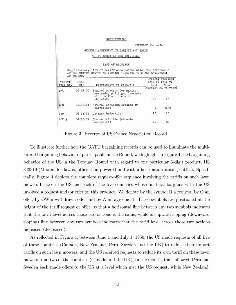
Figure 3: Excerpt of US-France Negotiation Record

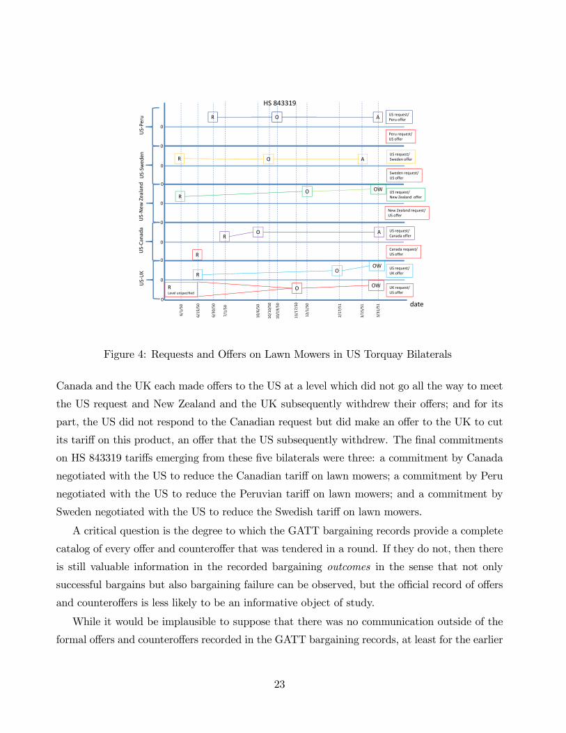
To illustrate further how the GATT bargaining records can be used to illuminate the multi-

lateral bargaining behavior of participants in the Round, we highlight in Figure 4 the bargaining

behavior of the US in the Torquay Round with regard to one particular 6-digit product, HS

843319 (Mowers for lawns, other than powered and with a horizontal rotating cutter). Specif-

ically, Figure 4 depicts the complete request-offer sequence involving the tariffs on such lawn

mowers between the US and each of the five countries whose bilateral bargains with the US

involved a request and/or offer on this product. We denote by the symbol R a request, by O an

offer, by OW a withdrawn offer and by A an agreement. These symbols are positioned at the

height of the tariff request or offer, so that a horizontal line between any two symbols indicates

that the tariff level across those two actions is the same, while an upward sloping (downward

sloping) line between any two symbols indicates that the tariff level across those two actions

increased (decreased).

As reflected in Figure 4, between June 1 and July 1, 1950, the US made requests of all five

of these countries (Canada, New Zealand, Peru, Sweden and the UK) to reduce their import

tariffs on such lawn mowers, and the US received requests to reduce its own tariff on these lawn

mowers from two of the countries (Canada and the UK). In the months that followed, Peru and

Sweden each made offers to the US at a level which met the US request, while New Zealand,

22

date

6/1/50

6/15

/50

6/30

/50

7/1/50

10/6/50

10/10/50

10/19/50

11/17/50

12/1/50

3/15

/51

US‐UK

US‐Canada

US‐New

 Zealand

US‐Sw

eden US request/

Sweden offer

Sweden request/US offer

US request/New Zealand  offer

US request/Canada offer

US request/UK offer

New Zealand request/US offer

Canada request/US offer

UK request/US offer

R

O

0

0

0

0

0

0

0

0

R

R

R

O

O

A

HS 843319

A

ORLevel unspecified

3/31

/51

OW

US‐Peru

0

0Peru request/US offer

US request/Peru offer

R

R

O A

OW

O

2/17

/51

OW

Figure 4: Requests and Offers on Lawn Mowers in US Torquay Bilaterals

Canada and the UK each made offers to the US at a level which did not go all the way to meet

the US request and New Zealand and the UK subsequently withdrew their offers; and for its

part, the US did not respond to the Canadian request but did make an offer to the UK to cut

its tariff on this product, an offer that the US subsequently withdrew. The final commitments

on HS 843319 tariffs emerging from these five bilaterals were three: a commitment by Canada

negotiated with the US to reduce the Canadian tariff on lawn mowers; a commitment by Peru

negotiated with the US to reduce the Peruvian tariff on lawn mowers; and a commitment by

Sweden negotiated with the US to reduce the Swedish tariff on lawn mowers.

A critical question is the degree to which the GATT bargaining records provide a complete

catalog of every offer and counteroffer that was tendered in a round. If they do not, then there

is still valuable information in the recorded bargaining outcomes in the sense that not only

successful bargains but also bargaining failure can be observed, but the offi cial record of offers

and counteroffers is less likely to be an informative object of study.

While it would be implausible to suppose that there was no communication outside of the

formal offers and counteroffers recorded in the GATT bargaining records, at least for the earlier

23

rounds there is reason to believe that the records offer a fairly complete catalog of the tendered

offers and counteroffers. This is so for two reasons. First, in older rounds such as the Torquay

Round that predated the ready use of electronic records and portable computing devices, a

written record of the detailed product-level bilateral tariff cutting proposals —proposals which

typically included dozens if not hundreds of product-level tariff cuts to be considered —was the

only way that a proposal or counter-proposal could be offered and assessed.11 Second, the final

bargaining outcomes in the GATT bargaining records predominantly emerge in a continuous

fashion from the recorded requests, offers and counteroffers, rather than appearing in the final

agreement as a new and never-before-recorded proposal —for example, over 95% of the exact

tariff bindings to which the US ultimately agreed in the Torquay Round first appear in the US-

Torquay bargaining records as either requests by US bargaining partners or as earlier US offers

to some bargaining partner —which is at least consistent with the lack of important informal

proposals being tendered outside of the recorded offers and counteroffers.12

There are a number of significant challenges that must be overcome before the GATT

bargaining data can be used for research. The Online Data Appendix covers these issues

in detail. The most challenging issue concerned creating product level concordances across

negotiations. Our solution was to concord product level descriptions into HS 1988 6-digit

codes. We henceforth refer to an HS6 code as a product.

5. Stylized Facts of GATT Tariff Bargaining

We now use data from the US bilaterals at Torquay to develop a number of stylized facts relating

to GATT tariffbargaining. While our subsequent data analysis in part helps to provide possible

interpretations for some of these stylized facts, our main purpose here is simply to identify the

facts. We start with an overview of the number of parties and the timing and frequency of

offers. We then state a set of stylized facts, focusing first on bargaining patterns alone and then

11We thank Sushan Demirjian, Deputy Assistant USTR for Market Access and Industrial Competitiveness,for pointing this out to us.12More specifically, only 44 out of the 988 tariff bindings to which the US agreed in its Torquay bilaterals

do not appear as either requests or earlier offers in some US bilateral; and this count reflects an upper bound,because the numbers are calculated at the HS6 level and a lack of match could (and does in each of the cases wehave checked) reflect changes in the 10 digit product mix in any given HS6 product category over the course ofthe bargain rather than the appearance of a tariff binding in the final agreement that did not appear somewherein the US bilateral bargaining records at an earlier date. That said, this statistic may be less informativeregarding the completeness of the bargaining records than it first appears, because as we discuss below there isvery little intensive-margin movement in the offers through time.

24

introducing trade data and expanding our focus to bargaining and trade patterns.

5.1. Timing and Offer Frequency

We begin with a helicopter view of the US-Torquay negotiations. There were 39 participating

countries in the Torquay Round.13 However, the Benelux Countries (a customs union consisting

of Belgium, Luxembourg and the Netherlands) negotiated their common external tariffs as a

single entity, reducing the total number of parties negotiating at Torquay to 37. Of the 666

possible bilaterals, 588 were initiated. The US was itself engaged in bilateral negotiations with

24 of its 36 potential negotiating partners (i.e., the US made initial requests of and/or received

initial requests from 24 of these countries).14 It reached final agreement with 15.

In Figure 5 we provide an overview of the timing and actions —request (R), modification

of request (RM), offer (O), modification of offer (OM), withdrawal of offer (OW), agreement

(A) and modification of agreement (AM) —for each of the 24 bilateral negotiations involving

the US at Torquay. The dates of each action are recorded on the horizontal axis. For each

US negotiating partner listed on the vertical axis, the bottom (blue) line displays the actions

relating to the US tariff —the offers by the US and the requests of its negotiating partners —

while the top (red) line displays the actions relating to the foreign negotiating partner’s tariff

—the requests by the US and the offers of its negotiating partners.

Figure 5 displays 57 dates, distributed across the 10 month period of the Torquay Round,

on which the US and/or at least one of its negotiating partners took an action in their bilateral.

Most of the dates involve multiple actions across a number of bilaterals. A couple of interesting

patterns stand out.

First, while the US and/or its negotiating partners took actions on 57 separate dates before

reaching a conclusion to the Round, Figure 5 reveals that the amount of back-and-forth within

any bilateral is much more limited, often consisting of only a couple of actions by each party

over the course of the Round and never more than a handful by either. Moreover, some bilateral

bargains appear to sit dormant for long periods of time and yet ultimately end in agreement.

13The countries were Australia (AU), Austria (AT), Benelux Countries —Belgium, Luxembourg, Netherlands—(BX), Brazil (BR), Burma (BU), Canada (CA), Ceylon (CE), Chile (CH), Cuba (CU), Czechoslovakia (CS),Denmark (DK), Dominican Republic (DO), Finland (FI), France (FR), Germany (DE), Greece (GR), Guatemala(GT), Haiti (HT), India (IN), Indonesia (ID), Italy (IT), Korea (KR), Liberia (LI), New Zealand (NZ), Nicaragua(NI), Norway (NO), Pakistan (PA), Peru (PE), Philippines (PH), Southern Rhodesia (RH), Sweden (SE), Syria-Lebanon (SL), Turkey (TR), South Africa (ZA), United Kingdom (UK), United States (US) and Uruguay (UR).14The countries present at Torquay with which the US did not negotiate were Burma, Ceylon, Chile, Finland,

Greece, Liberia, Nicaragua, Pakistan, Philippines, Southern Rhodesia, Syria-Lebanon and Uruguay.

25

Figure5:TimingofActionsintheUSTorquayBilaterals

26

For example, Figure 5 shows that the US and Denmark exchanged initial offers on 11/8/1950,

made no modifications to their requests of or offers to each other after that date, and reached a

final agreement on 3/31/1951. A possible interpretation is that the initial proposals contained

the elements of a final agreement, but the details of the final agreement hinged on details of

other bilaterals that had yet to be concluded. Relatedly, a number of the initial offers were not

tabled until midway through the round, possibly reflecting issues of sequencing across bilaterals.

Finally, there are a number of agreements that are themselves modified late in the round (AM).

One interpretation of these modifications is that they reflect the kinds of adjustments that stage-

4 of the Torquay Protocol anticipated might be necessary as information became available about

other agreements that were concluded in the round.

This pattern points to important multilateral dimensions of the bargaining, whereby large

numbers of separate bilateral bargains, each with small numbers of moves, were linked together

into an interrelated fabric. We will later offer evidence that countries sought multilateral reci-

procity in their negotiations, which would introduce an important multilateral dimension into

each country’s bargaining and therefore be consistent with our interpretation of this pattern.

A second interesting pattern revealed by Figure 5 is that, subsequent to 10/1/1950 when

the bilateral bargaining stage of the Torquay Round began, virtually all the back-and-forth

occurs on offers rather than requests. That is, countries choose overwhelmingly (in fact, with

only one exception) to make counter-proposals by modifying their own-tariff-cut offers rather

than modifying the tariff-cut requests they make of their bargaining partners.

This pattern warrants future study, but one possibility is again that it may reflect important

multilateral dimensions of the bargaining. For example, if a country is attempting to achieve

a balance in its bilaterals that is consistent with multilateral reciprocity, it is likely to be more

straightforward for the country to modify its own offers in order to achieve this balance than

to attempt to achieve balance by requesting modifications to its bargaining partners’offers,

because the ramifications of such requests for the bargaining partners with regard to their

other bilaterals are likely to be unknown to the country making these requests.

5.2. Stylized Facts: Bargaining Patterns

We now record and document six stylized facts relating to GATT bargaining patterns.

Stylized Fact 1: While the set of requests a country entertains seems to conform with what

might be expected on the basis of the principal supplier rule, when it comes to deciding which

27

bargaining partners to make requests of on a given product there appears to be a more narrow

focus than principal supplier considerations alone would dictate.

Table 1 details the number of HS6 level product categories involved in negotiations for US

tariff cuts (“sales,” in the top panel) and negotiating partner tariff cuts (“purchases,” in the

bottom panel). The first column reports the number of HS6 products across all negotiating

partners, the second column reports the number of HS6 product-negotiating partner pairs,

and the third through sixth columns report summary statistics by negotiating partner on the

number of HS6 products.

We may conclude from the first and third rows of the top panel in Table 1 that on aver-

age the requests received by the US and the offers made by the US reflect a high degree of

concentration across exporting countries, with somewhere between 1 and 2 exporting countries

typically bargaining with the US over a given US tariff reduction. Under the assumption (which

we will confirm below with the US import data) that the larger export suppliers of a product

into a market are the suppliers usually involved in the bargaining over access to the market for

that product, this in turn implies that typically it is the largest 1 or 2 export suppliers into

the US market on a given product that are engaged in negotiations over the US tariff in that

market, consistent with the principal supplier rule. But the bottom panel of Table 1 seems to

tell a different story. The US was one of the largest trading economies of the day, and while

product-level by-country export data for the period is not currently available, it seems likely

that, when the US was among the largest export suppliers of a product into one country, it

would have enjoyed similar status for that product in the markets of many countries.15 And

yet, the first and third rows of the bottom panel in Table 1 indicate that on average the US

singled out just a couple of countries in its Torquay bargaining attempts to lower foreign tariffs

on any given product. It therefore appears that something beyond principal supplier status is

limiting the cross-country scope of US bargaining efforts at Torquay.

Table 2 provides further evidence on this point. This table shows that, for both US sales (i.e.,

for requests and offers that refer to US tariffs) and US purchases (i.e., for requests and offers

that refer to the tariffs of US bargaining partners), the modal HS6 level product category was

under negotiation with only one partner. At the same time, Table 2 indicates that a significant

number of HS6 level product categories were at play with multiple numbers of negotiating

15While we have the relevant trade data in electronic form, the necessary concordances have yet to be created.This is a major undertaking, and it is the focus of ongoing work.

28

partners, indicating important direct linkages across negotiations. In particular, the left panel

indicates that, of the HS6 products on which the US received a request, it received a request

from only one trading partner on 57% of these products but received requests from more than

three trading partners on only 7% of these products. Similarly, of the HS6 products on which

the US made an offer, it made the offer to only one trading partner on 65% of these products

but made the offer to more than three trading partners on only 4% of these products, with the

corresponding percentages for successful offers being 78% and 1% respectively. Turning to the

right panel of Table 2 we see that, of the HS6 products on which the US made a request, it made

its request of only one trading partner on 51% of these products and made requests from more

than three trading partners on 17% of these products. Similarly, of the HS6 products on which

the US received an offer, it received the offer from only one trading partner on 54% of these

products and received an offer from more than three trading partners on 14% of these products,

with the corresponding percentages for successful offers being 64% and 5% respectively.

There is a rightward shift of the distribution between the left and right panels of Table

2 as would be expected for a large country such as the US that is likely to be the principal

supplier of products into multiple foreign markets. But what is surprising is how small this

rightward shift is, again indicating that something beyond principal supplier status seems to be

limiting the cross-country scope of US bargaining efforts at Torquay. An interesting question,

which we leave for future research, is whether strategic elements in the GATT tariff bargaining

environment could account for this.

Stylized Fact 2: Substantial numbers of offers are made that were not requested by the country

to which the offer is extended. In significant numbers of cases, these offers are made without a

request from any bargaining partner.

Again from Table 1, while the US entertained requests for tariff cuts on 2,586 HS6 products,

it offered tariff cuts on 1,769 HS6 products, 1,357 of which correspond to HS6 products that

were requested by some bargaining partner, and 412 of which correspond to products that

were not requested by any bargaining partner. And while the US requested tariff cuts from

its bargaining partners on 2,298 HS6 products, it received offers on 1,844 HS6 products, 1,595

of which corresponded to HS6 products that it had requested, and 249 of which corresponded

to HS6 products that it had not requested. Moreover, of the 2,635 initial offers that the US

made across its bargaining partners, 1,107 of these were made to bargaining partners on HS6

products which they themselves had requested, while the remaining 1,528 of these were made

29

to bargaining partners on HS6 products that they themselves had not requested; by contrast,

of the 3,665 initial offers that the US received from its bargaining partners, 2,793 of these were

received from bargaining partners that were responding to a US request on this HS6 product,

while the remaining 872 of these were received from bargaining partners that had not received

a US request on this HS6 product.

In the end, as Table 1 reveals, the US agreed to final concessions on 1,260 of the 1,769 HS6

products that it had offered, while its bargaining partners agreed to final concessions in their

bilaterals with the US on 1,505 of the 1,844 HS6 products that they had offered the US. Most,

but not all, products that reached a final agreement were initially requested: 23.7% of the

agreed US tariff cuts were on HS6 products that were not requested by its negotiating partners,

while 13.5% of the tariff cuts agreed to by US negotiating partners in their bilaterals with the

US were on HS6 products that were not requested by the US.

Stylized Fact 3: The numbers of back-and-forth offers and counter-offers in any bilateral

bargain are relatively small, and for some bargains the initial offers sit dormant on the table

for long periods of time and are then finalized with a single modification at the time that other

bargains are concluded.

Stylized Fact 4: While in principle a proposal can be altered by either modifying the tariff

commitment requested of one’s bargaining partner or modifying the own-tariff commitment of-

fered to the bargaining partner, in practice the mechanics of altering proposals through time

overwhelmingly takes the form of modifications to offers rather than modifications of requests.

As we have noted, Figure 5 reveals the long periods of dormancy in some bilaterals and

the almost complete absence of modified requests once the bilateral bargaining stage has been

reached. In Tables 3 and 4 we present evidence on the amount of “back and forth”offers and

counter-offers during negotiations, with Table 3 focused on US sales (i.e., for requests and offers

that refer to US tariffs) and Table 4 focused on US purchases (i.e., for requests and offers that

refer to the tariffs of US bargaining partners).

As Table 3 shows, on HS6 products for which the US made at least one offer in the bilateral,

the maximum number of offers it made on that product is 3 and the average is 1.6; for requests

the analogous numbers are 2 and 1.16 Conditional on a final agreement reached on that HS616For example, a product might be included in an initial offer, and then also be in the set of products that

is included in a modified offer, and then later the offer on this product might be withdrawn, in which case wewould record that a total of 3 offers were made on this product.

30

product in that bilateral, the maximum number of offers the US made on that product is again

3 but the average is now 2; and for requests the analogous numbers are still 2 and 1. Table 3 also

reports the data on the simple counts of US offers and counter-offers for a country pair (but not

also per good). For bilaterals where the US made at least one offer, the average number of US

offers per bilateral is 2.6, with a maximum number of 5, and conditional on a final agreement

reached between the two countries in that bilateral the analogous numbers are 3.1 and 5. And

the analogous numbers of US requests for a country pair are an average of 1.2 and a maximum

of 3 independently of whether or not a final agreement is reached. Table 4 shows the analogous

information for the requests and offers that refer to the tariffs of US bargaining partners, and

depicts broadly similar patterns. Models of strategic delay in bargaining (e.g., Admati and

Perry, 1987, and Cramton, 1992) predict small numbers of offers and counter-offers broadly

in line with our findings here, though these models cannot be applied directly to settings of

bilateral bargaining with externalities such as ours.

Stylized Fact 5: The bargaining appears to have taken the form of essentially take-or-leave

offers on the intensive margin (the level of the tariff cut offered) and back-and-forth offers and

counter-offers on the extensive margin (which products are to be included in the bargain).

Table 5 describes the magnitude of the tariffconcessions requested and offered for US “sales”

(i.e., for requests and offers that refer to US tariffs) and US “purchases”(i.e., for requests and

offers that refer to the tariffs of US bargaining partners). This table reports statistics by HS

code —country pair; and it conditions on finalized agreed concessions being reached. As the top

row reveals, the average tariff cut requested from the US by its bargaining partners amounted

to roughly a 40% cut in the existing (ad valorem and specific) US tariff, while the average tariff

cut requested by the US of its bargaining partners amounted to approximately a 30% cut in

their existing (ad valorem and specific) tariff level. The bottom rows show that the tariff cuts

that the US actually agreed to amounted to on average a 32% cut in its existing tariff, whereas

the tariff cuts that the US was able to convince its bargaining partners to agree to amounted

to on average roughly an 11% cut in their existing tariff.

The middle three rows of Table 5 reveal that the levels of the initial offers in effect determined

the levels of the finalized concessions. For both US sales and US purchases, these averages reveal

an apparent lack of adjustment along the intensive margin between the initial offers and the

finalized concessions. In Table 6 we provide additional evidence that changes on the intensive

margin were small in magnitude. Unlike Table 5, Table 6 reports statistics by HS code but

31

does not condition on country pair; and it does not condition on finalized concessions being

reached. As Table 6 reflects, for US sales the average final offer was very close to the initial

offer (US purchases in Table 6 reflect movements across US bargaining partners, and so are not

informative about this feature).17 Finally, we return to Table 1 and now focus on the fourth row,

which describe the degree of adjustments to offers at the extensive margin over the course of

the Torquay Round.18 After the initial offer and prior to a final agreement, the US modified its

offers on roughly 12% of the HS6 products on which it made an initial offer, and US bargaining

partners modified their offers to the US on approximately 14% of the HS6 products for which

they made initial offers. Together these tables indicate that the most important dimension for

negotiations was on the extensive margin, that is dropping and/or adding products from the

negotiation, whereas there was minimal adjustment taking place on the intensive margin, that

is, in the size of the tariff cuts being offered on any particular product. Moreover, 99.5% of the

product-level offers that the US made over the course of the round are contained in its initial

set of offers, indicating that at least for the US these extensive margin adjustments appear to

be essentially a reallocation of a fixed set of offers across bargaining partners.

Figure 6 demonstrates extensive margin movement in one detailed example, the US-Italy

17Of course, our focus on the averages reported in Tables 5 and 6 ignores the fact that the standard deviationsare fairly substantial. But we believe that the size of the standard deviation is largely being driven by outliersassociated with the maximum values listed in the table, which are themselves explained by our aggregation tothe HS6 level. For example, in the US-German bilateral, the initial US offer made on 10/16/1950 for “Nail,barbers’and animal clippers, and blades: valued at more than $1.75 per dozen,”which falls into HS6 851020,was to bind its tariff at a 10% ad valorem level, and this same tariff level was included in its final offer dated3/21/1951. But the US subsequently modified its final offer to Germany on 3/31/51, and in that modificationit (a) maintained its offer of a 10% ad valorem tariff on “Nail, barbers’and animal clippers, and blades: valuedat more than $1.75 per dozen,” but also added (b) an offer to bind its tariff on “Nail, barbers’ and animalclippers: valued not over 50 cents per dozen”at the level of 1.75% ad valorem and (c) an offer to bind its tariffon “Nail, barbers’and animal clippers: valued over 50 cents but not over $1.75 per dozen”at the level of 7.5%ad valorem, and both of these product categories also fall into HS6 851020. Hence, in this case our HS6 measurewould indicate substantial intensive margin movement of the HS6 851020 tariff between the initial US offer andthe (modified) final US tariff, when in fact at the 10 digit product level there is no intensive margin movementand only an extensive margin movement.18As the second rows of Table 1 indicates, after the initial request and prior to final agreement, the US

modified its requests on approximately 19% of the HS6 products on which it made initial requests, and USbargaining partners modified their requests of the US on approximately 3% of the HS6 products for which theymade initial requests. Recalling however the observation in the context of our discussion of Figure 5 that onlyone modification of requests occurred across the US bilaterals subsequent to the exchange of initial offers andthe beginning of bilateral bargaining, it follows that subsequent to the exchange of initial offers virtually all ofthe extensive margin adjustments occur on the offer side, with modifications of only a fraction of a percent forUS requests of its bargaining partners (corresponding to the US modification of its requests of France) and nomodifications of the requests of the US by its bargaining partners over this period. For this reason, we do notemphasize this extensive margin adjustment in the text.

32

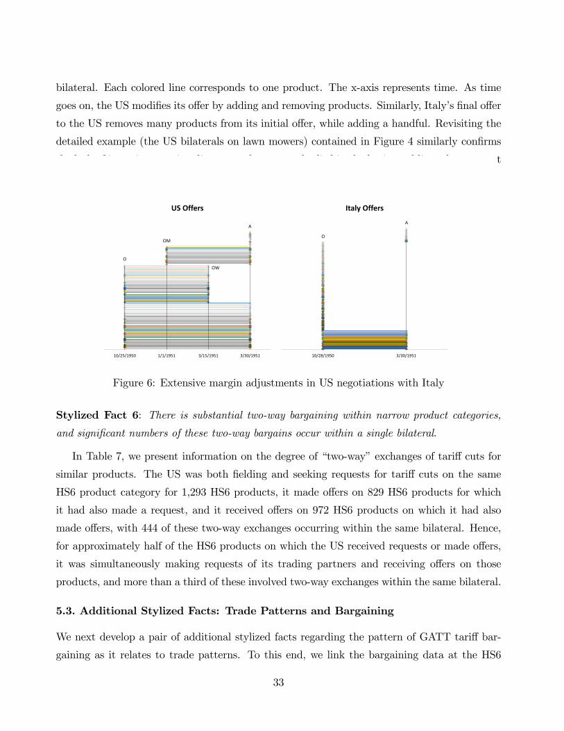
bilateral. Each colored line corresponds to one product. The x-axis represents time. As time

goes on, the US modifies its offer by adding and removing products. Similarly, Italy’s final offer

to the US removes many products from its initial offer, while adding a handful. Revisiting the

detailed example (the US bilaterals on lawn mowers) contained in Figure 4 similarly confirms

the lack of intensive margin adjustment there, as embodied in the horizontal lines that connect

each offer (O) that ends in agreement (A).

10/25/1950 1/1/1951 3/15/1951 3/30/1951

US Offers

O

OM

OW

A

10/28/1950 3/30/1951

Italy Offers

A

O

Figure 6: Extensive margin adjustments in US negotiations with Italy

Stylized Fact 6: There is substantial two-way bargaining within narrow product categories,

and significant numbers of these two-way bargains occur within a single bilateral.

In Table 7, we present information on the degree of “two-way”exchanges of tariff cuts for

similar products. The US was both fielding and seeking requests for tariff cuts on the same

HS6 product category for 1,293 HS6 products, it made offers on 829 HS6 products for which

it had also made a request, and it received offers on 972 HS6 products on which it had also

made offers, with 444 of these two-way exchanges occurring within the same bilateral. Hence,

for approximately half of the HS6 products on which the US received requests or made offers,

it was simultaneously making requests of its trading partners and receiving offers on those

products, and more than a third of these involved two-way exchanges within the same bilateral.

5.3. Additional Stylized Facts: Trade Patterns and Bargaining

We next develop a pair of additional stylized facts regarding the pattern of GATT tariff bar-

gaining as it relates to trade patterns. To this end, we link the bargaining data at the HS6

33

level to US import values from 1948 compiled in the Census Bureau’s United States Imports for

Consumption of Merchandise report. This report provides import values by 7-digit Schedule A

product category-country in 1948 current dollars into the US. We concord Schedule A codes to

HS6 codes by text analysis and manual inspection to link to the bargaining data.

From these data, we calculate the Herfindahl-Hirschmann concentration index (HHI) of

suppliers into the US and the fraction of supply coming from trading partners that were absent

at Torquay. We further link these data to the Rauch (1999) indices of product differentiation

where we assign a product to be undifferentiated if it is either traded on an exchange or features

a reference price. Finally, we link by HS4 code to the trade elasticities estimated in Broda et

al. (2008) to use as a measure of product level market power. We make use of these additional

variables in our data analysis of the next section, where we also discuss limitations associated

with these variables.

The summary statistics for the trade and trade-related variables are in Table 8. The products

on which the US made tariff-cut offers or received requests at Torquay are broadly similar on

observable dimensions to the full set of products.

Stylized Fact 7: The largest suppliers of a product into a market are usually involved in the

negotiations over the tariff on that product in that market.

In Table 9 we use the trade data together with the bargaining data to confirm an important

and widely acknowledged feature of GATT tariff bargaining: the largest supplying interests

are usually involved in the bargain. The top left-hand panel of Table 9 provides one way to

gauge the importance of the largest suppliers in the negotiations. The first row reports the

number and fraction of HS6 products offered by the US that did not include an offer to the

top ranked Torquay supplier of that HS6 product into the US market, the second row reports

the number and fraction of HS6 products offered by the US that did not include an offer to

either the first or second ranked Torquay supplier of that HS6 product into the US market, and

so on. As the numbers indicate, for roughly 79% of the HS6 products that the US offered at

Torquay, at least one of the top 2 Torquay suppliers of that HS6 product into the US market

received an offer on that HS6 product. The bottom left-hand panel displays the same measure

based on “overall”(i.e., whether or not at Torquay) ranking of suppliers, and shows that, for

roughly 68% of the HS6 products that the US offered at Torquay, at least one of the top 2

overall suppliers of that product into the US market received an offer on that HS6 product.

The right-hand panels of Table 9 display the same measures, but for requests of the US made by

34

its bargaining partners. The numbers in the right-hand panels show that the largest supplying

interests were also important in generating requests, though not as important as their role in

generating offers.19

Stylized Fact 8: There can be a significant role in the negotiations for smaller suppliers of a

product into a market where the largest suppliers are not involved.

We next use the trade and bargaining data to illustrate a less-appreciated point: despite

the dominant role of the largest suppliers in negotiations, there can be a significant role for

the smaller suppliers when the largest suppliers are not involved. This can be seen with the

measures we present in Table 10 when those measures are compared with the measures in Table

9. The top left panel of Table 10 depicts the number and fraction of HS6 offers that the US

made to the Nth ranked Torquay supplier of that HS6 product into the US market.20 For

example, as can be seen from Table 10, roughly 40% of the US offers are made to suppliers

ranked 3rd or lower, roughly 26% of the US offers are made to suppliers ranked 4th or lower,

roughly 16% of the US offers are made to suppliers ranked 5th or lower, and roughly 11% of the

US offers are made to suppliers ranked 6th or lower. The question we wish to ask is, what is

the role played by these lower-ranked suppliers when they receive an offer: Are they the biggest

suppliers involved in the negotiations?; Or are they secondary players that receive an offer on

the HS6 product that has also been made to a larger supplier? The answer is suggested by

comparing the numbers in the top left panel of Table 10 to those in the top left panel of Table

9. Specifically, as the numbers in Table 9 show, roughly 21% of the HS6 products offered by the

US are made when only the 3rd and lower-ranked Torquay suppliers are involved, and roughly

11% of the HS6 products offered by the US are made when only the 4th and lower-ranked

suppliers are involved. This suggests that, when they are involved, the 3rd- and 4th- ranked19In principle the total numbers of HS6 products offered and requested in Table 9 should correspond to the

numbers in the “Unique” column of Table 1, but in fact the totals underlying Table 9 are smaller. This isbecause calculating the rankings in Table 9 requires that HS6 imports into the US are strictly positive, andthis is not always true in the 1948 import data, with such HS6 products then excluded from Table 9. The offermeasures on the left-hand-side panels of Table 9 are probably overstated due to aggregation to the HS6 level.When the measures are recalculated on the subsample of data for which we have 7-digit schedule A codes, eachof the fractions is roughly cut in half (the request measures on the right-hand side seem to be unaffected byaggregation). This, of course, only strengthens our claim. The column sums of the entries in Table 9 will belarger than the total numbers of HS6 products offered and requested that underlie the statistics presented inTable 9, because for example an HS6 product that is not offered to the first or second ranked supplier would becounted in both the first row and the second row of Table 9.20The total numbers of HS6 offers and requests in Table 10 should in principle correspond to the numbers in

the “Total”column of Table 1, but as with the corresponding comparison in Table 9, the totals in Table 10 aresmaller, for the same reason as explained in note 19.

35

Torquay suppliers sometimes play a primary role in the negotiations, in the sense that they

are the largest suppliers receiving a US offer on the HS6 product under negotiation. Similar

conclusions regarding overall supplier rank and requests follow from an examination of the other

panels of Table 10 in comparison with those of Table 9.21

6. Multilateral versus Bilateral Reciprocity

As we noted in the Introduction, GATT reports from the early rounds emphasize that a key

feature of GATT relative to earlier attempts to negotiate MFN tariff reductions (e.g., the US

Reciprocal Trade Agreements Act) is that the multilateral nature of GATT allowed countries

to relax their need for strict bilateral reciprocity (“balance”) in negotiations and focus instead

on achieving reciprocity on a multilateral basis. As the report describing the results of the 1947

Geneva Round put it:

...The multilateral character of the Agreement enabled the negotiators to offer more

extensive concessions than they might have been prepared to grant if the concessions

were to be incorporated in separate bilateral agreements. Before the Geneva negotiations

a country would have aimed at striking a balance between the concessions granted to

another country and the direct concessions obtained from it without taking into account

indirect benefits which might accrue from other prospective trade agreements; it might

even have been unwilling to grant an important concession if it had been obliged to extend

that concession to third countries without compensation. (ICITO, 1949, p. 10)

Was the relaxation of strict bilateral reciprocity afforded by the multilateral nature of the

GATT bargaining forum a key to GATT’s success? One way to assess this claim would be

to attempt direct measures of the degree to which the GATT bargaining outcomes violated

21The percentages we report in Tables 9 and 10 might overstate the role of smaller suppliers because thesepercentages are based on the 1948 US import data, and some countries (e.g. Germany) may appear to be smallsuppliers only because the 1948 data reflects World War II disruptions of normal trade patterns. To checkfor this possibility, we collected and concorded the 1938 US import data and recalculated the percentages inTables 9 and 10 based on this prewar period. These percentages show an even greater role of smaller suppliers,suggesting that the impacts of World War II are not creating a false sense of the importance of smaller suppliersin the Torquay negotiations. A second possibility is that aggregation of the US import data to the HS6 level maydisguise the importance of some suppliers at the tariff-line level. We have spot checked this second possibilityby using the 7 digit Schedule A 1948 US import data, and have found that the apparent role of small suppliersis indeed reduced under these calculations. Nevertheless, even by these calculations the role of smaller suppliersremains more than just a curiosum, which is why in the text we emphasize this role.

36

bilateral reciprocity but conformed with multilateral reciprocity. A diffi culty with attempting

a direct assessment of this kind is that it requires knowledge of detailed trade elasticities that

would apply to the countries involved in the GATT negotiations during the period in which

they were negotiating.22

Here we develop an alternative approach to assessing this claim. In particular, if countries

were counting on indirect trade benefits from the MFN tariff cuts negotiated between third

parties to achieve multilateral reciprocity in the Torquay Round, then we might expect to see

reactions in the bilateral bargaining records of some countries when an unexpected event occurs

in the bilateral negotiations of other countries (whereas according to the theory sketched out

in 2.2 no such reaction would be expected if strictly bilateral reciprocity had been demanded

and achieved all along). Indeed, a report issued by the GATT Secretariat in the aftermath of

the failure of the UK and its Commonwealth partners to reach agreement with the US in the

Torquay Round suggests that such reactions to unexpected third-party events were thought to

be an important feature of the round:

The fact that certain of the more important negotiations initiated between existing

contracting parties did not result in agreements inevitably had some reactions on other

negotiations. If, for example, the other countries engaged in tariff negotiations at Torquay

had been sure that substantial concessions were going to be exchanged between the United

Kingdom, Australia and New Zealand on the one hand, and the United States on the other,

they might have been prepared, in the light of the benefits which they would have enjoyed

from the automatic extension of these concessions to them, to go somewhat further in

reducing their own tariffs. Substantial cuts in the tariffs of these Commonwealth countries,

however, would inevitably have involved substantial reductions in some of the margins of

preference which they accord to one another and the Commonwealth negotiators were not

22In the next subsection we will make use of trade elasticities for the US estimated by Broda, Limao andWeinstein (2008) under the assumption that the cross-product pattern of these elasticities applied to the periodrelevant to the Torquay Round, but this approach would have to be expanded to all trading countries of the timein order for us to use it to assess reciprocity directly, and elasticity estimates for many of the countries are notavailable. An additional diffi culty with direct assessment of reciprocity is the prevalence of quotas during theTorquay period (often rationalized by dollar shortages and balance of payment exceptions). As Curzon (1966;pp. 70-1, pp. 85-6, Chapter VI) describes, quotas were regularly used in early round eras by many countriesother than the US, which accounted in part for the willingness of countries to offer major tariff cuts in the firstcouple of rounds but which makes it diffi cult to draw a tight connection between tariff cuts and trade volumechanges for these other countries. The concern is that tariff cuts were coincident with greater use of quotas, asa substitute instrument.

37

prepared to agree to major tariff concessions of this kind at the price which the United

States negotiators were prepared to offer in return. (ICITO, 1952, p. 9)

This discussion suggests an indirect way to evaluate the importance of the relaxation of the

need for strict bilateral reciprocity in contributing to the success of GATT tariff bargaining. If

the collapse of the bilateral bargains between the US on the one hand and the UK and a number

of its Commonwealth partners on the other triggered significant changes in the remaining

bilaterals that the US negotiated with third countries at Torquay, then this would be evidence

that strict bilateral reciprocity was not a feature of the bargains that were anticipated to prevail

on the eve of this collapse, and evidence therefore consistent with the view that the relaxation

of strict bilateral reciprocity which was facilitated by the GATT multilateral bargaining forum

was indeed important to the success of the GATT approach.23 On the other hand, if little or

no change in the remaining US bilaterals is observed in response to this collapse, this would

suggest that bilateral reciprocity between the US and each of its bargaining partners was in

fact built in to the negotiations all along, and that the relaxation of the need for strict bilateral

reciprocity facilitated by the GATT multilateral bargaining forum was not a central reason for

GATT’s success.

We follow this logic with two tests. First, we check whether the US-UK breakdown led to

a retrenchment of offers by US bilateral partners at the country level. Second, we test at the

product level whether goods which were under negotiation with the UK prior to the breakdown

were more likely to be re-offered to other countries after the breakdown.

To implement these tests, we must identify when the news of the US-UK/Commonwealth

breakdown occurred. This news was offi cially announced at the GATT Secretariat on March

31, 1951, but the New York Times (1951) broke the news with a dateline March 30 special

press report, and it seems unlikely that even the March 30 announcement would have come as

23To further relate this interpretation to our theoretical analysis in section 2.2, we make two additionalobservations. First, if the failure of the US/UK bargain is regarded as random and exogenous, then undermultilateral reciprocity any resulting changes in US proposals might be broadly interpreted as the utilization ofan alternative dominant strategy for the US. Second, we note that the simple theory sketched out in section 2.2does not explain why the relaxation of bilateral reciprocity in favor of multilateral reciprocity would matter tothe success of tariff bargaining. Alternative models, however, may provide potential explanations. For example,as suggested in the Introduction, in a 3-good, 3-country model of triangular trade, where country A exports gooda to country B, country B exports good b to country C, and country C exports good c to country A, negotiationsover import tariffs can generate potential gains under multilateral reciprocity but not under bilateral reciprocity.More generally, empirical evidence of a beneficial role for multilateral reciprocity may motivate interesting andnew theoretical analyses.

38

a complete surprise to the other negotiating countries at Torquay. Below we will report results

that set the “news”date at February 18, because that was the day after the last action in the US-

UK bilateral —the UK’s modification of its offer to the US on 2/17/1951 —and it seems plausible

that general news of the disappointing UK response to the US request that it substantially

reduce the margins of preference which it accorded to its Commonwealth partners would have

become known to other negotiators soon after. But we also experiment with alternative news

dates between March 1 and March 30.

We begin with the question: Did the willingness of US bargaining partners to make offers

in their bilaterals with the US diminish once it was known that the US-UK/Commonwealth

bilaterals had failed? Fixing 2/18/1951 as the date by which negotiators at Torquay had learned

that the US-UK/Commonwealth bilaterals would fail, we calculate the total number of HS6

product-country pairs with an existing tariffoffer to the US outstanding on 2/18/1951, summed

across all US bilaterals except the US-UK, US-Australia and US-New Zealand bilaterals. This

number is 2,333. We then calculate the total number of HS6 product-country pairs with a final

tariff offer to the US at the end of the Round, again summed across all US bilaterals (with the

failures of the US-UK, US-Australia and US-New Zealand bilaterals excluding these bilaterals

automatically from this sum). This number is 2,396. Clearly, comparing these two numbers

would not lead one to conclude that there had been a diminished willingness on the part of US

bargaining partners to make offers in their bilaterals with the US after they had learned that

the US-UK/Commonwealth bilaterals would end in failure. Performing this same calculation

with the “news”date fixed at either 3/1/1951 or 3/30/1951 yields similar results.

However, on closer examination this simple difference is driven strongly by a suite of offers

from France after the US-UK/Commonwealth breakdown. While these offers from France may

have been influenced by the US-UK breakdown, the narrative from the time suggests that other

factors unique to the France-US negotiation were probably more decisive.24 Eliminating France

from the calculation produces a total number of outstanding offers to the US of 2,282 before

and 1,856 after 2/18/1951, a result that is consistent with the position that countries were

24In particular, as Curzun (1966, p. 110) describes, France was alone in following a strategy at Torquaythat relied heavily on threats of renegotiating the existing tariff concessions it had agreed to in prior GATTrounds (under the GATT renegotiation provisions contained in Article XXVIII that we described in section2.2). Curzun notes that most countries renegotiated less than ten items, whereas France was the exceptionand “renegotiated some 200 items, only to find later, to quote one of her negotiators, ‘that it had neither beennecessary nor worthwhile.”’This discussion raises the possibility that France abandoned this strategy late inthe round, which may account for the large number of offers it made to the US subsequent to 2/17/1951.

39

counting on indirect trade benefits from the MFN tariff cuts negotiated between the US and its

UK/Commonwealth bargaining partners to achieve (multilateral) reciprocity, and pulled back

on their offers to the US in an attempt to reestablish reciprocity once they realized that these

indirect benefits would not be forthcoming.

We next turn to the question: Did the failure of the US-UK/Commonwealth bilaterals lead

the US to extend its offers to countries directly on products where those countries had antici-

pated that they would gain access indirectly into the USmarket through the US-UK/Commonwealth

bilateral? We estimate the following regression on the sample of HS6 codes for which the US

made an offer.

USOffPosti,f = αHS1 + γf + β1USOffUKAUNZi + β2 log(1 + USImpi) + (6.1)

β3 log(1 + USImpi,f ) + β4 log(1 + USImpUKAUNZi) + εif

where we include HS1 fixed effects, negotiating partner fixed effects, and condition on total US

import volume, bilateral volume from each non-Commonwealth US negotiating partner, and

volume from the Commonwealth countries. The key coeffi cient in equation (6.1) is β1 which, if

positive, indicates that a good was more likely to be offered after the US-UK/Commonwealth

breakdown if it was part of the outstanding set of offers that the US had extended to the UK

and its Commonwealth partners.

Table 11 provides the regression evidence (OLS and Probit), with the news date fixed at

2/18/1951. The coeffi cient on USOffUKAUNZ is positive and significant in all specifications,

as would be expected if the failure of the US-UK/Commonwealth bilaterals led the US to

extend its offers to countries directly on products where those countries had anticipated that

they would gain access indirectly into the US market through the US-UK/Commonwealth

bilaterals. Using news dates of 3/1/1951 and 3/15/1951 yields similar results, while if the

offi cial 3/30/1951 dateline of the New York Times press release is used for the news date, the

results are still significant in the Probit, but overall the relationship is weaker. The results are

robust to excluding offers to France.

Overall, these results provide indirect evidence that news of the breakdown in the US-

UK/Commonwealth bilaterals caused 3rd countries to rebalance their bilaterals with the US, and

hence evidence that bilateral reciprocity was not a feature of the bargains that were anticipated

to prevail on the eve of this collapse, consistent with the view that the relaxation of bilateral

40

reciprocity which was facilitated by the GATT multilateral bargaining forum was important for

the success of the GATT approach. Our results provide support for the view expressed in the

report by the GATT Secretariat quoted above, that this rebalancing took the form of a general

retrenchment of offers to the US. However, this interpretation is contingent on treating the

US-France negotiations as unique, as described above. If one treats the US-French negotiations

as the same as others, our results suggest that this rebalancing was achieved by reorienting US

offers directly to those 3rd countries who would have stood to gain the most indirectly from

successful US-UK/Commonwealth bargains, and there was no overall retrenchment of offers.

7. Bargaining under Reciprocity and MFN

The theoretical analysis developed in section 2 highlights the potential value of recasting the

GATT multilateral bargaining problem as a collection of simultaneous bilateral bargains that

adhere strictly to the twin pillars of reciprocity and MFN. In particular, we have shown there

that this structure eliminates bargaining externalities across bargaining pairs, and that it is

then a dominant strategy for each country to truthfully reveal its (effi cient-under-symmetry)

politically optimal reaction curve tariffs on a product-by-product basis.25 An implication is

that, by comparing initial offers to the final agreed tariff concessions in the round, we can

construct measures of the success of the Torquay Round.26

Accordingly, we now assume that the US satisfied strict multilateral reciprocity and MFN in

its Torquay tariff bargaining.27 Given this assumption, and defining the set O as the set of allHS6 products for which the US made an offer at Torquay, we can then use the union of the US

initial offers in each of its Torquay bilaterals, denoted by τUS Offeri for product i ∈ O, to identifythe set of politically-optimal-reaction-curve tariffs for the US in the Torquay Round. Denoting

25Recall that we also assume throughout that self-enforcement constraints do not bind at the politically-optimal-reaction-curve tariffs.26In principle, by imposing additional structure we could use this result to recover government preferences and

construct the complete-information effi ciency frontier for the round, against which the actual outcome of theround can be judged and the performance of counter-factual bargaining protocols can be assessed. For example,adopting the political economy model of Grossman and Helpman (1994), the assumption of strict adherence toreciprocity and MFN would allow us to utilize the initial offers from a given GATT round to estimate the valuethat each government places on lobby contributions along the lines of Goldberg and Maggi (1999), and withthese estimates we could then construct the effi ciency frontier for the round. This would require data from allof the bilaterals of a given round, however, and so we leave this more ambitious program for future research.27Entering into the Torquay negotiations the US did maintain a small number of tariff preferences (e.g., on

sugar imports from Cuba), but by the conclusion of the Torquay Round the US had terminated even these tariffpreferences and maintained only MFN tariffs (see United Nations, 1952, p. 204).

41

the politically-optimal-reaction-curve tariffs for the US by τUS RPO

i , we therefore impose

τUS RPO

i = τUS Offeri ∀ i ∈ O. (Assumption 1)

We then characterize the degree of tariff bargaining failure at the product level for the US in

the Torquay Round by a dummy variable TorqFailUSi that takes the value 1 if the US did not

reach agreement on product i at Torquay and 0 if the US did reach an agreement on product i.

Implicit in our discussion of bargaining failure is the assumption that all US offers that

should be made on effi ciency grounds are in fact made, and therefore that for i /∈ O US tariffsare already at their politically optimal levels. Below we will relax this assumption and allow

that bargaining failure may also take the form of US offers that are not made. As a separate

matter, we could characterize the degree of bargaining failure with a continuous variable that

measures the distance between the initial US offer and the final agreed US tariff. But as we have

established in section 5, conditional on an agreement occurring there is almost no movement

on the intensive margin between the initial offer and the final agreed tariff, so our dichotomous

bargaining failure variable TorqFailUS captures the relevant variation in the data.

Our goal is now to understand the patterns of US bargaining failure as displayed by

TorqFailUS with factors that could introduce bargaining frictions —and thereby potentially

account for this failure —but would not invalidate Assumption 1. To this end, we consider the

following seven factors:

(i) Bargaining Externalities: As a partial check on our assumption that the US satisfied

strict multilateral reciprocity and MFN in its Torquay tariff bargaining, we include a measure

of foreign exporter concentration on the right-hand side of the failure equation, and check

to see whether there is evidence that the US faced a free-rider problem. If, as we assume,

the US abides by MFN and its bargains satisfy strict multilateral reciprocity, then bargaining

externalities should not arise and the US should not face a free rider problem.28 But under MFN,

if multilateral reciprocity is not achieved, there will be 3rd−party externalities and free riderproblems could arise, the more so the less concentrated are the foreign supplier-countries into the

US market.29 To perform this check, we use the US bilateral import data from 1948 as described

28Of course, bargaining externalities might still arise if the export supply adjustments embedded in thedefinition of reciprocity are realized gradually over time. Third-party externalities might then be experiencedin the short run. Our simple model abstracts from these considerations as a first pass.29See Ludema and Mayda (2013) for related ideas regarding the impact of supplier-country concentration on

the free rider problem.

42

in the previous section to create the following variable: for each US product i we construct

the Herfindahl-Hirschmann concentration index among all Torquay-country suppliers of that

product into the US market. We denote this variable by EXT . If the US faces a significant

free-rider problem among the supplier-countries at Torquay (we consider supplier-countries not

at Torquay below), EXT should be negatively related to our measure of US bargaining failure:

the higher our measure of exporter-country concentration into the US market, the smaller the

free-rider problem and the lower the chance of US bargaining failure. Finding this negative

relationship would be evidence against our Assumption 1, while a failure to find this negative

relationship would constitute evidence consistent with Assumption 1.

It might be thought that the relationship between bargaining success and the concentration

of export suppliers is hard-wired into GATT negotiations by the principal supplier rule. Recall,

though, that the definition of principal supplier contained in the original 1947 GATT bargaining

protocol and quoted above in section 3 explicitly provides for the possibility of defining principal

supplier status based on the cumulative trade share of countries present at Torquay even if no

single country alone has a principal supplying interest, suggesting that it was anticipated that

concentration of the suppliers present at a round need not be the critical factor in bargaining

success of failure. Our theoretical results point to reciprocity as a potential force for overcoming

the free-rider issue even when the concentration of suppliers is not high.

(ii) UK Preferential Trade Agreements: US bargaining failures could be associated

with the existence of tariff preferences in the UK. This reflects the well-known possibility of a

“stumbling block” relationship between PTAs and multilateral liberalization, but the partic-

ular mechanism here is novel: for the UK and its Commonwealth partners, such preferences

would violate MFN and lead thereby to the possibility of strategic behavior in the US/UK and

US/UK-Commonwealth bilateral bargains; and this possibility of strategic behavior in turn

potentially could result in bargaining failures for the US in products where the UK or UK-

Commonwealth countries are a principal supplier into the US market. As long as the US does

not itself have preferences and hence abides by MFN (and expects multilateral reciprocity),

Assumption 1 still holds; thus, the US would continue to have a dominant strategy in which

it offers its politically-optimal-reaction-curve tariffs. The UK and its Commonwealth partners,

however, might have additional strategic considerations when making their tariff offers, since

their tariffs may generate 3rd−party externalities due to the PTAs in which they participate. As

43

a consequence, their tariff offers may differ from their politically-optimal-reaction-curve tariffs.

In this way, such PTAs may act as stumbling blocks to GATT/WTO multilateral liberalization

because they introduce strategic considerations into the GATT bargaining setting that are not

present for countries that abide by MFN.30 Making use of the US bilateral import data from

1948, we check for this possibility by asking if a dummy variable —whose ith value is 1 when

either the UK or a UK-Commonwealth country is a principal supplier into the US market of

product i and 0 otherwise —is positively related to our measure of US bargaining failure. We

denote this dummy variable by PTA.

(iii) Barter: US bargaining failures could be associated with the lack of a double coinci-

dence of wants that barter requires, again a possibility that would not invalidate Assumption

1. To check for this, we make use of the bargaining and 1948 US import data to construct a

variable whose ith value is the ratio of the number of HS6 product requests that the US makes of

the largest volume exporter to which the US made an offer on product i, relative to (1 plus) the

number of such HS6 product offers that the US made to that country. We denote this variable

by WANT . For a product i where this measure is low, the double coincidence of wants needed

for the US to successfully complete a bargain over its tariff on product i is likely to be lacking,

and bargaining failure could result for that reason. Hence, we expect that WANT should be

negatively related to our measure of US bargaining failure.

(iv) Preserving Bargaining Power for Future Rounds: It is possible that US bar-

gaining failures could be associated with the degree to which countries absent from the Torquay

Round constitute principal suppliers of product i, measured by the share of 1948 US imports

of product i that are supplied by countries not present at the Torquay Round. We denote this

variable by ABSENT . The absence of principal suppliers from Torquay would not invalidate

Assumption 1; and whether or not it would lead to bargaining failure as we have defined it

would depend in part on whether the US could make use of the so-called “split-concessions”

bargaining technique that Beckett (1941) claims was utilized by the US in the context of the

US Reciprocal Trade Agreements Act. If the absence of principal suppliers from Torquay does

30The Benelux countries were also members of a PTA. But unlike the UK Commonwealth, theirs was acustoms union, and following arguments similar to those in Bagwell and Staiger (1999, 2001) it can be shownthat customs unions do not invalidate our dominant strategy arguments made in section 2 and therefore shouldnot be the source of any particular bargaining frictions.

44

result in bargaining failure, then we would expect to find that ABSENT is positively related

to our measure of US bargaining failure.

(v) Previously Bound Tariffs The Torquay Round was the third GATT bargaining

round, and by the beginning of this round the US had in place a set of tariff commitments

to which it had agreed over the first two rounds.31 It is possible that the presence of previ-

ously bound tariffs could help predict the likelihood of bargaining failure at Torquay in several

ways. One possibility is simply that a previous tariff binding indicates that the ineffi ciency in

the level of that tariff has been largely addressed in previous rounds, and there is little left

to bargain over for that tariff. Under this possibility, we would expect that the presence of

previously bound US tariffs would increase the chance of bargaining failure. But “gradualism,”

whereby the reductions on a single tariff are purposefully spread over many rounds, is a widely-

acknowledged feature of GATT tariff liberalization. And from this perspective the presence

of previously bound US tariffs might be expected to predict a reduced chance of bargaining

failure at Torquay, because the early success suggests that the ingredients for success in further

negotiated reductions in that tariff are also likely in place.32 To allow for these possibilities,

we create the variable PREV BND, which is defined as a dummy variable whose ith value is

1 if the US has a pre-existing GATT tariff commitment on product i at the beginning of the

Torquay Round and 0 otherwise. If the gradualism effect dominates, then we would expect to

find that PREV BND is negatively related to our measure of US bargaining failure.

(vi) Differentiated Goods: Recently Ossa (2014) has argued that the existence of dif-

ferentiated goods can interfere with the ability of MFN and reciprocity to neutralize 3rd−party31As Hoda (2001, pp. 84-85) describes and as we have noted above, the tariff bindings negotiated in the

first (Geneva 1947) round came up for renewal during the Torquay Round and could have been the subject ofArticle XXVIII renegotiations under a parallel process at Torquay. In principle these renegotiations might beimportant for understanding the broader tariff negotiations at Torquay, but the derestricted GATT bargainingdata does not yet include records on any of the renegotiations that occurred. However, as Hoda notes, the USmade statements that it did not wish to invoke Article XXVIII during the Torquay negotiations, and in the endthe US carried out discussions for “certain adjustments”under Article XXVIII on just 3 product-level tariffs.Given our focus on the US bilaterals at Torquay, it therefore seems unlikely that the lack of Article XXVIIIbargaining records would substantially undercut our ability to understand the bargaining behavior of the US inthe Torquay Round.32Whether or not evidence of gradualism would be consistent with our Assumption 1 would depend on the

reasons for gradualism. Gradual tariff reductions that reflect split concessions and the gradual accession ofcountries through time would not pose a problem for Assumption 1, but gradualism that reflects the evolutionof binding self-enforcement constraints (see for example Staiger, 1995, Devereux, 1997 and Bond and Park,2002) could invalidate Assumption 1.

45

externalities. This suggests that US bargaining failures (stemming from bargaining externali-

ties) could be associated with the presence of differentiated goods imported into the US, even if

the US abides by MFN and achieves strict multilateral reciprocity in its Torquay bargains. Of

course, in the presence of product differentiation, the scope of application of the MFN principle

becomes critical: At what point do differentiated products cease to become “like products,”

and thereby not require a common tariff treatment under the MFN principle? The answer to

this question is important in the present context, because as Ossa demonstrates the magnitude

of the 3rd−party externality is directly proportional to the degree of product differentiationover which the MFN principle applies (inversely proportional to the elasticity of substitution

across the products), and so the externality should be small to the extent that like products are

narrowly defined for purposes of the MFN principle.33 Nevertheless, to allow for this possibility

we use the Rauch (1999) index concorded to each 1948 US import product i, and denote a

product as undifferentiated if the Rauch index lists the product as being traded on an exchange

or having a reference price.34 We denote this variable by UNDIFF . Based on Ossa’s findings,

we would expect to find that UNDIFF is negatively related to our measure of US bargaining

failure.

(vii) Market Power The terms-of-trade theory predicts that the goods for which nego-

tiated reductions in tariffs are the most attractive are those for which the conceding country

holds more market power. This suggests that a given level of bargaining frictions would be

less likely to lead to US bargaining failure over product i the greater the US market power in

product i, and hence the greater the potential surplus from agreement. We therefore condition

on market power using the log inverse foreign export supply elasticity (log(ωi)) as estimated

by Broda, Limao, and Weinstein (2008) for the US at the HS4 level, and we expect to find

that log(ωi) is negatively related to our measure of US bargaining failure. We apply the HS4

level estimate to all HS6 codes within the HS4 description, and emphasize that this measure

is estimated with trade data covering the 1990’s and early 2000’s which is much later than our

period of interest. Thus we are making the strong assumption that the relative magnitudes of

33As illustrated for example in note 17, the product lines on which individual tariffs are defined and withinwhich MFN would apply can be and often are quite detailed and narrowly defined.34We treat products which do not have a Rauch index as differentiated. Dropping these observations does

not meaningfully change the results we present, however we lose a substantial number of observations in thatcase. Needless to say, applying the Rauch index to data from 1948 requires a large leap of faith. We discussthis further in note 35 below.

46

these elasticities across goods has not changed over the relevant time period.35

Finally, as noted above we have thus far imbedded into our discussion of bargaining failure

the assumption that all US offers that should be made on effi ciency grounds at Torquay were in

fact made, and therefore that US tariffs are already at their politically optimal levels for i /∈ O.But it is reasonable to expect that the US might have targeted certain kinds of offers at Torquay

and left others for future rounds: for example, it was well known at the time that a major goal

of the US at Torquay was to use its tariff offers to bargain down the external MFN tariffs of

Commonwealth countries and thereby achieve a reduction in the margin of tariff preferences

that they offered to each other. And it also seems reasonable to expect that the US may have

refrained from making tariff offers even when its tariffs were set above their politically optimal

levels if it thought that those offers would fail with high probability. DefiningM as the set of

HS6 products which the US imported in 1948, and defining TorqOfferUSi as a dummy variable

whose ith value is 1 if the US made an offer at Torquay on product i ∈ M and 0 otherwise,

we therefore estimate an “offer equation” in addition to our “failure equation,”to allow that

bargaining failure may also take the form of offers that are not made.36

Collecting these points, we estimate the following regressions:

TorqOfferUSi = βHS1 + β1EXTi + β2EXT2i + β3PTAi + β4WANTi (7.1)

+β5ABSENTi + β6UNDIFFi + β7 log(ωi) + β8REQi + β9PREV BNDi + εi

TorqFailUSi = αHS1 + α1EXTi + α2EXT2i + α3PTAi + α4WANTi (7.2)

+α5ABSENTi + α6UNDIFFi + α7 log(ωi) + α8REQi + α9PREV BNDi + εi

where equation (7.1) is a Probit for whether the US makes an offer on product i ∈M, and where

equation (7.2) is a linear probability model of whether product i ∈ O, on which the US made an35To the extent that this mis-measurement and the analogous mis-measurement associated with our use of

the Rauch (1999) index for the 1948 import data is random across products, we would expect it to attenuatethe results we find. A more subtle form of mis-measurement could arise whereby the US granted concessions onproducts that were on their way to having centralized exchanges, or whose market power was trending upward.Future research could use the data we are collecting across GATT rounds to re-estimate elasticities from thistime period.36We also check whether accounting for selection into offers affects the failure equation.

47

offer at some point during Torquay, ultimately resulted in a final concession. The variable REQi

is a dummy variable for whether the US received a request from a counterparty at Torquay to

reduce its tariff on product i, and βHS1 and αHS1 are HS1 fixed effects.37 The WANTi variable

in the offer equation is constructed slightly differently from the WANTi variable in the failure

equation as we described that variable above. Specifically, for the offer equation WANTi is

constructed as a variable whose ith value is the ratio of the number of HS6 product requests

that the US makes of the largest volume exporter from which the US received a request on

product i, relative to (1 plus) the number of such HS6 product requests that the US received

from that country. Finally, we include both EXTi and EXT 2i in each equation to allow for the

possibility that free-rider effects might vary non-linearly with exporter-country concentration.

The results from estimating equation (7.1) and (7.2) are contained in Table 12. The first

four columns present the results of estimation with log(ωi) omitted, and the last four columns

present the estimation with log(ωi) included (and a roughly 10% reduction in the sample size

due to the exclusion of products for which log(ωi) is unavailable). In both sets of specifications,

we also check robustness with respect to different assumptions on accounting for selection

into offers in the failure equation. The second and fifth columns do not include any selection

correction. The third and sixth columns include the inverse Mills ratio from the offer equation,

but do not exclude any other variables in the failure equation. The fourth and eighth exclude

REQ and HS1 fixed effects from the failure equation. Across these specifications, we do not

find evidence that selection into offers significantly affects the results of the failure equation;

nonetheless, we focus on the results where we account for selection, and exclude REQ and HS1

fixed effects from the failure equation.38 Most of the coeffi cients of interest are significant and

37We also include λ̂i, the estimated inverse Mills ratio from the Probit to correct for non-random selectionof products into offers, as the failure regression is conditional on there being an initial offer. However, we findthat this correction does not affect our results.38The inclusion of REQ and HS1 in the offer equation are based on the following observations: (i) for any tariff

that the US government wished to offer up for negotiations at Torquay, it had to secure tariff-cutting authorityfrom Congress by the October 1 date at which the offer stage of the Torquay Round bargaining was set tocommence, (ii) there are political costs to securing tariff-cutting authority, (iii) these political costs are higherfor tariffs that have not been requested by any trading partner, because US exporters cannot then be pittedagainst US import-competing interests to mitigate the costs, and (iv) these political costs vary by industry. Theexclusion of these variables from the failure equation then follows based on the view that, once authority tomake tariff-cutting offers has been granted, these particular costs have been borne and so they do not impactthe probability of offer failure. That we find no evidence of selection into offers could of course be an indicationthat our offer equation is poorly specified. But it could also indicate that US offers were largely determinedby US tariff-cutting authority, and that offer-failure probabilities were very diffi cult for the US government topredict at the time that it was seeking this tariff-cutting authority.

48

of the expected sign. A couple of specific points are noteworthy.

First, focusing on the failure equation (columns 4 and 8 of Table 12), there is strong evidence

of a positive relationship between bargaining failure and the concentration of Torquay-country

suppliers into the US market, the opposite of what would be expected if the free-rider problem

were present. This relationship appears to be non-linear, and it turns slightly negative for very

high levels of concentration (when there exists a single supplying country whose share among

Torquay suppliers into the US market exceeds 90%). A possible interpretation of the positive

relationship is that a lower concentration of Torquay country suppliers implies greater numbers

of potential suppliers to whom an offer could be made, with only one successful offer required

to avoid failure. But the central message of the failure equation estimates regarding bargaining

externalities and the free-rider problem is that there is little if any evidence for the negative

relationship between EXT and our measure of US bargaining failure that would be expected if

the free-rider problem is present. Turning to the offer equation (columns 1 and 5 of Table 12),

the estimates imply that for low levels of supplier concentration a rise in the concentration of

Torquay country suppliers increases the likelihood of an offer, possibly indicating the presence

of a free-rider problem at low levels of Torquay supplier concentration; but for concentration

levels beyond a mid-level threshold, higher concentration reduces the chances of an offer, again

the opposite of what would be expected if the free-rider problem were present.

We interpret these coeffi cient estimates as together providing substantial support for the

position that the free-rider problem among those countries present at Torquay was likely not

a major issue for the US in its Torquay negotiations. This interpretation is in turn consistent

with our Assumption 1 and broadly supports the view that the US abided by MFN and strict

multilateral reciprocity in the Torquay Round. That said, our coeffi cient estimates do point to

the existence of a free-rider issue for offers at low levels of concentration, suggesting that an

important task of future research is to confront the complications associated with 3rd−partyexternalities that arise when adherence to reciprocity and/or MFN is not strict.

A second noteworthy finding from Table 12 concerns the impact of PTAs. As would be

expected based on the bargaining-friction stumbling block arguments described above, columns

4 and 8 of Table 12 imply that US bargaining failure is more likely for products that are

principally supplied to the US market by the UK and its Commonwealth partners (though

this effect loses significance when log(ωi) is included). On the other hand, the offer equations

in columns 1 and 3 indicate that PTAs stimulate offers, a finding that is consistent with the

49

emphasis placed by the US on reducing the size of within-Commonwealth tariff preferences by

bargaining down their external MFN tariffs at Torquay.39 Hence, our estimates indicate that

PTAs can have two counter-acting effects: they can stimulate offers, and in this way can be

seen as “building blocks”of negotiated MFN tariff reductions, but they also make those offers

more likely to fail and in this way are stumbling blocks to the multilateral system. The overall

effect of PTAs in the Torquay Round —that is the impact on generating successful offers and

hence final agreed tariff concessions —can be gauged by evaluating the net effect of these two

forces for each observation in our sample and taking the mean of the net effects. When we

do this using the estimates in columns 1 and 4 of Table 12, we find that the probability of a

final agreed US tariff concession in the Torquay Round rises from roughly 0.36 when PTAs are

absent to 0.41 in the presence of PTAs, which amounts to a sizable building block effect.

Finally, Table 12 also indicates a strong positive relationship between US market power and

the likelihood and likely success of US offers at Torquay (consistent with the terms-of-trade

theory), a strong positive relationship between previous US tariff bindings and the likelihood

and likely success of US offers at Torquay (consistent with a gradualism story), a strong posi-

tive impact on the likelihood of offers when the double coincidence of wants needed for barter

to occur is present, and a strong positive relationship between the degree of product differen-

tiation and the likelihood of bargaining failure. This last result is in line with Ossa’s (2014)

prediction, and provides further support for the view that allowing for 3rd−party externalitiesin the analysis of GATT tariff bargaining is an important task for future research.40

8. Conclusion

Our initial look at the Torquay Round bargaining records has shown that GATT multilateral

tariff bargaining displays an array of interesting features. We document that governments

39This finding is also consistent with a view often expressed by trade policy practitioners at the time of theearly GATT rounds, that multilateral GATT negotiations were a needed response to the formation of PTAs.For example, in remarks made before the Joint Economic Committee, former Secretary of State Christian Herterappealed to the formation of the European Community (EC) in 1957, and the phase-in of the EC customs unionamong the original six EC countries over the next decade and the prospect of an integrated EC market that thisimplied, as a key reason that the US should push for a new GATT round of multilateral tariff negotiations (seeHerter, 1961). The US efforts in this regard led eventually to the initiation of the Kennedy Round of GATTnegotiations in 1964. That said, our finding that PTAs stimulate offers is reversed when we re-estimate theregressions in Table 12 using the 1938 US import data (see also note 21), and so we view the results in Table12 as suggestive of a possible building block effect but not conclusive.40Our evidence on gradualism may also point to the importance of this task for future research, especially if

the reasons for gradualism relate to self-enforcement constraints (see also note 32).

50

bargain with back-and-forth offers on the particular tariffs they are willing to cut, but they

make take-or-leave offers on the depth of these cuts. They make counter-proposals by adjusting

the set of tariff cuts they are willing to offer in light of the cuts offered by their bargaining

partners, but they do not propose adjustments to what their bargaining partners have offered.

The big supplying countries play the dominant role in negotiations, but the role of smaller

supplying countries can also be significant. Initial offers sometimes sit dormant on the table

for long periods of time and are then finalized with a single modification at the time that other

bargains are concluded.

We also show that tariff cuts are more likely to be offered on products where the country has

substantial market power, and that these offers are more likely to succeed. We find evidence

that tariff cuts are more likely to be offered by a country when members of a PTA from

which that country is excluded have a principal supplying interest; and while these offers are

individually less likely to succeed, on net PTAs generate greater numbers of successful offers and

hence appear to be building blocks rather than stumbling blocks for MFN tariff liberalization.

We find little evidence of a major free-rider problem associated with the bilateral-bargaining-

under-MFN approach that GATT has frequently adopted in its rounds of multilateral tariff

bargaining. And we use the breakdown of the US-UK bilateral midway through the Torquay

Round as a natural experiment to provide novel evidence that GATT’s ability to facilitate

multilateral reciprocity indeed aided liberalization.

Many of these features seem consistent with the predictions of the terms-of-trade theory of

trade agreements, as we have detailed above. We have built on the implications of this theory in

our analysis but we have left the full exploitation of these implications for future work.41 Some

of the features seem to reflect a more general bargaining environment, however, and point to

the importance of more general theoretical structures and additional theoretical work to guide

the analysis and interpret the results. All of these features would be unknowable without the

detailed bargaining data that the WTO has begun to make publicly available. In this light, as

more and more of this data becomes accessible to researchers, we view our initial look at the

GATT bargaining data as providing a promising view for the road ahead.

41For example, as we mentioned (see note 26), we could with some additional structure recover governmentpreferences and map out the international effi ciency frontier, and use this to evaluate the performance of counter-factual bargaining protocols.

51

References

Admati, Anat R. and Motty Perry (1987), “Strategic Delay in Bargaining,”Review of Economic

Studies, LIV, 345-364

Bagwell, Kyle and Robert W. Staiger (1999), “An Economic Theory of GATT,”American Economic

Review 89(1): 215-48

Bagwell, Kyle and Robert W. Staiger (2001), “Reciprocity, Non-discrimination and Preferential

Agreements in the Multilateral Trading System,”European Journal of Political Economy, June

Bagwell, Kyle and Robert W. Staiger (2002), The Economics of the World Trading System, Cam-

bridge, MA: The MIT Press

Bagwell, Kyle and Robert W. Staiger (2005), “Multilateral Trade Negotiations, Bilateral Oppor-

tunism and the Rules of GATT/WTO,”Journal of International Economics 67(2): 268-94

Bagwell, Kyle and Robert W. Staiger (2010a), “The WTO: Theory and Practice,”Annual Review of

Economics, 2: 223-56

Bagwell, Kyle and Robert W. Staiger (2010b), “Backward Stealing and Forward Manipulation in the

WTO,”Journal of International Economics, 82(1): 49-62

Bagwell, Kyle and Robert W. Staiger (2011), “What do trade negotiators negotiate about? Empirical

evidence from the World Trade Organization,”American Economic Review 101(4): 1238-73

Beckett G (1941), The Reciprocal Trade Agreements Program. New York: Columbia Univ. Press

Bond E, Park J-H (2002), “Gradualism in trade agreements with asymmetric countries,”Review of

Economic Studies 69: 379-406

Bown, Chad P. and Meredith A. Crowley (2013), “Self-Enforcing Trade Agreements: Evidence from

Time-Varying Trade Policy,”American Economic Review 103(2): 1071-1090

Broda, Christian, Nuno Limao, and David E. Weinstein (2008), “Optimal Tariffs and Market Power:

The Evidence,”American Economic Review, 98(5): 2032-65

Cramton, Peter (1992), “Strategic Delay in Bargaining with Two-Sided Uncertainty,” Review of

Economic Studies, 59(1): 205—225

52

Crawford, Gregory S., and Ali Yurukoglu (2012), “The Welfare Effects of Bundling in Multichannel

Television Markets,”American Economic Review, 102(2): 643-85

Curzon, Gerard (1966), Multilateral Commercial Diplomacy: The General Agreement on Tariffs and

Trade and its Impact on National Commercial Policies and Techniques, Praeger: New York

Devereux, M.B. (1997), “Growth, Specialization, and Trade Liberalization,”International Economic

Review, 38(3)

Estevadordal, Antoni, Caroline Freund, Emanuel Ornelas (2008), “Does regionalism affect trade

liberalization toward nonmembers?,”Quarterly Journal of Economics 123(4): 1531-75

Goldberg, Pinelopi and Giovanni Maggi (1999), “Protection for Sale: An Empirical Investigation,”

American Economic Review, 89(5): 1135-55

Gowa, Joanne and Soo Yeon Kim (2005), “An Exclusive Country Club: The Effects of the GATT

on Trade, 1950-94,”World Politics, 57(4): 453-478

Grossman, Gene M. and Elhanan Helpman (1994), “Protection for Sale,”American Economic Review

84(4): 833-50

Herter, C. (1961), Statement before the Joint Economic Committee of the Congress of the United

States, December 4-14, pp. 8-13

Hoda, Anwarul (2001), Tariff Negotiations and Renegotiations under the GATT and the WTO:

Procedures and Practices, WTO and Cambridge University Press

Irwin, Douglas A. (1995), “The GATT in Historical Perspective,”American Economic Review Papers

and Proceedings 85 May: 323-328

Interim Commission for the ITO (1949), The Attack on Trade Barriers: A Progress Report on the

Operation of the General Agreement on Tariffs and Trade. Geneva, August

Interim Commission for the ITO (1952), GATT in Action: Third Report on the Operation of the

General Agreement on Tariffs and Trade. Geneva, January

Karacaovali Baybars and Nuno Limao (2008), “The Clash of Liberalizations: Preferential vs. Multi-

lateral Trade Liberalization in the European Union,”Journal of International Economics 74(2):

299-327

53

Keniston, Daniel (2013), “Bargaining and Welfare : A Dynamic Structural Analysis of the Autorick-

shaw Market,”Working Paper

Larsen, Bradley (2013), “The Effi ciency of Dynamic, Post-Auction Bargaining: Evidence fromWhole-

sale Used-Auto Auctions,”Working Paper

Limao, Nuno (2006), “Preferential Trade Agreements as Stumbling Blocks for Multilateral Trade

Liberalization: Evidence for the U.S.,”American Economic Review 96(3): 896-914

Limao, Nuno (2007), “Are Preferential Trade Agreements with Non-trade Objectives a Stumbling

Block for Multilateral Liberalization?”Review of Economic Studies 74(3): 821-55

Ludema, Rodney D. and Anna Maria Mayda (2009), “Do Countries Free Ride on MFN?,”Journal

of International Economics 77(2): 137-50

Ludema, Rodney and Anna Maria Mayda (2013), “Do Terms-of-Trade Effects Matter for Trade

Agreements? Theory and Evidence from WTO countries,” Quarterly Journal of Economics

128(4)

Mayer Wolfgang (1981), “Theoretical Considerations on Negotiated Tariff Adjustments,” Oxford

Economic Papers 33(1): 135-53

Ossa, Ralph (2014), “Trade Wars and Trade Talks with Data,”American Economic Review 104(12):

4104-46

Rauch, James E. (1999), “Networks Versus Markets in International Trade,”Journal of International

Economics 48(1) : 7-35

New York Times (1951), “U.S.-British Trade Talks Fail: Imperial Preference Blamed,”Special Press

Report to the New York Times by Michael L. Hoffman, dateline March 30; published March 31

Staiger, Robert W. (1995), “A Theory of Gradual Trade Liberalization,”in Deardorff, A., Levinsohn,

J., and Stern, R. (eds.) New Directions in Trade Theory, Univ of Mich Press

United Nations (1952), Treaties and International Agreements Registered or Filed and Recroded with

the Secretariat of the United Nations, Vol 144 No 814 (VIII)

WTO Appellate Body (2004), United States-Anti-Dumping Act of 1916– Recourse to arbitration by

the United States under 22.6 of the DSU. WT/DS136/ARB, 24 February

54

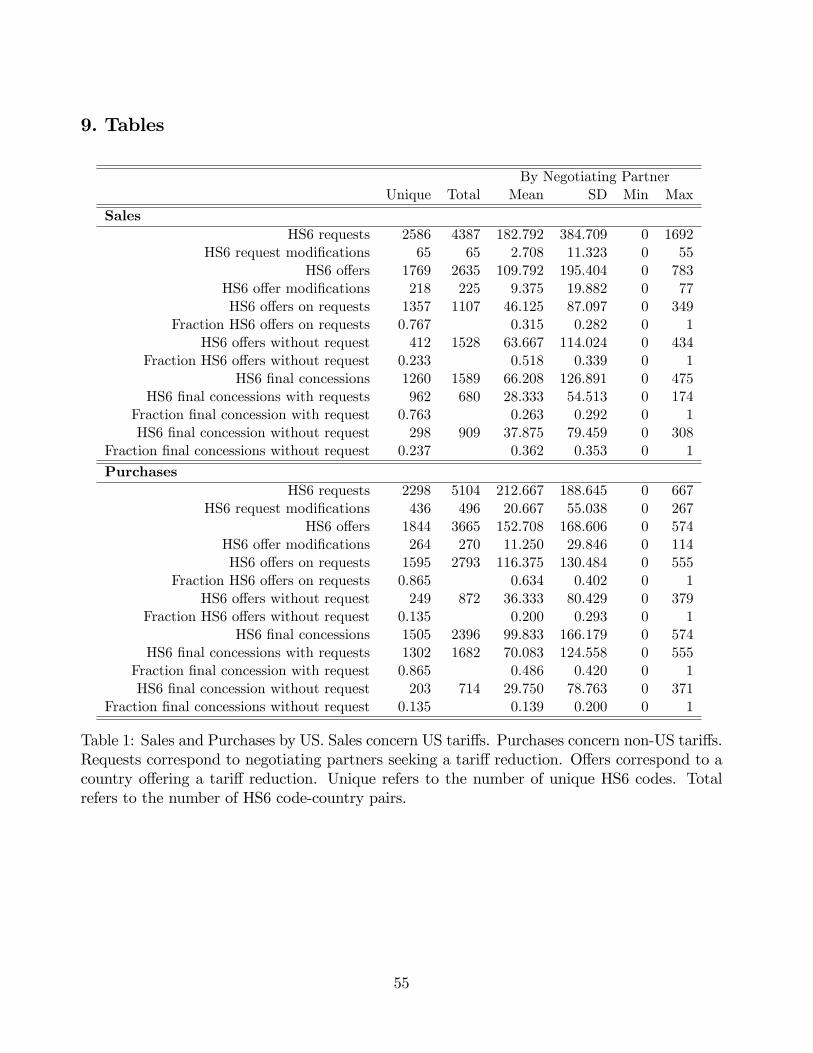
9. Tables

By Negotiating PartnerUnique Total Mean SD Min Max

SalesHS6 requests 2586 4387 182.792 384.709 0 1692

HS6 request modifications 65 65 2.708 11.323 0 55HS6 offers 1769 2635 109.792 195.404 0 783

HS6 offer modifications 218 225 9.375 19.882 0 77HS6 offers on requests 1357 1107 46.125 87.097 0 349

Fraction HS6 offers on requests 0.767 0.315 0.282 0 1HS6 offers without request 412 1528 63.667 114.024 0 434

Fraction HS6 offers without request 0.233 0.518 0.339 0 1HS6 final concessions 1260 1589 66.208 126.891 0 475

HS6 final concessions with requests 962 680 28.333 54.513 0 174Fraction final concession with request 0.763 0.263 0.292 0 1HS6 final concession without request 298 909 37.875 79.459 0 308

Fraction final concessions without request 0.237 0.362 0.353 0 1

PurchasesHS6 requests 2298 5104 212.667 188.645 0 667

HS6 request modifications 436 496 20.667 55.038 0 267HS6 offers 1844 3665 152.708 168.606 0 574

HS6 offer modifications 264 270 11.250 29.846 0 114HS6 offers on requests 1595 2793 116.375 130.484 0 555

Fraction HS6 offers on requests 0.865 0.634 0.402 0 1HS6 offers without request 249 872 36.333 80.429 0 379

Fraction HS6 offers without request 0.135 0.200 0.293 0 1HS6 final concessions 1505 2396 99.833 166.179 0 574

HS6 final concessions with requests 1302 1682 70.083 124.558 0 555Fraction final concession with request 0.865 0.486 0.420 0 1HS6 final concession without request 203 714 29.750 78.763 0 371

Fraction final concessions without request 0.135 0.139 0.200 0 1

Table 1: Sales and Purchases by US. Sales concern US tariffs. Purchases concern non-US tariffs.Requests correspond to negotiating partners seeking a tariff reduction. Offers correspond to acountry offering a tariff reduction. Unique refers to the number of unique HS6 codes. Totalrefers to the number of HS6 code-country pairs.

55

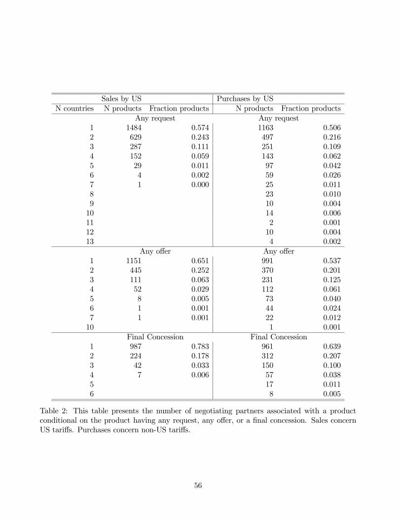
Sales by US Purchases by USN countries N products Fraction products N products Fraction products

Any request Any request1 1484 0.574 1163 0.5062 629 0.243 497 0.2163 287 0.111 251 0.1094 152 0.059 143 0.0625 29 0.011 97 0.0426 4 0.002 59 0.0267 1 0.000 25 0.0118 23 0.0109 10 0.00410 14 0.00611 2 0.00112 10 0.00413 4 0.002

Any offer Any offer1 1151 0.651 991 0.5372 445 0.252 370 0.2013 111 0.063 231 0.1254 52 0.029 112 0.0615 8 0.005 73 0.0406 1 0.001 44 0.0247 1 0.001 22 0.01210 1 0.001

Final Concession Final Concession1 987 0.783 961 0.6392 224 0.178 312 0.2073 42 0.033 150 0.1004 7 0.006 57 0.0385 17 0.0116 8 0.005

Table 2: This table presents the number of negotiating partners associated with a productconditional on the product having any request, any offer, or a final concession. Sales concernUS tariffs. Purchases concern non-US tariffs.

56

Mean SD Min MaxUnconditional

N offers per good-country 1.617 0.558 1 3N offers per country 2.550 1.356 1 5

N requests per good-country 1.003 0.054 1 2N requests per country 1.150 0.489 1 3

Conditional on final agreementN offers per good-country 1.965 0.379 1 3

N offers per country 3.067 1.163 2 5N requests per good-country 1.009 0.094 1 2

N requests per country 1.214 0.579 1 3

Table 3: Sales by US: This table presents statistics on the amount of back and forth on goodsand with negotiating partners over US concessions.

Mean SD Min MaxUnconditional

N offers per good-country 1.433 0.538 1 5N offers per country 2.100 1.071 1 6

N requests per good-country 1.005 0.074 1 2N requests per country 1.545 0.596 1 3

Conditional on final agreementN offers per good-country 1.639 0.546 1 5

N offers per country 2.400 1.056 2 6N requests per good-country 1.008 0.088 1 2

N requests per country 1.733 0.594 1 3

Table 4: Purchases by US: This table presents statistics on the amount of back and forth ongoods and with negotiating partners over concessions from the negotiating partner.

57

Sales PurchasesAd Val Specific All Ad Val Specific All

Initial Request N 1402 716 2118 2788 2117 4905over Mean 0.615 0.648 0.626 0.645 0.820 0.721

Existing Tariff SD 0.167 0.199 0.179 0.202 0.244 0.238Min 0.000 0.000 0.000 0.000 0.000 0.000Max 1.000 1.000 1.000 1.000 1.000 1.000

Initial Offer N 423 197 620 691 953 1644over Mean 1.192 1.155 1.181 1.472 1.193 1.310

Initial Request SD 0.505 0.825 0.624 0.683 0.500 0.600Min 0.033 0.000 0.000 0.000 0.000 0.000Max 5.000 10.000 10.000 5.000 6.667 6.667

Finalized Concession N 399 167 566 543 924 1467over Mean 1.195 1.083 1.162 1.291 1.190 1.227

Initial Request SD 0.541 0.560 0.549 0.444 0.531 0.503Min 0.033 0.000 0.000 0.000 0.000 0.000Max 5.000 4.571 5.000 3.571 8.000 8.000

Finalized Concession N 1267 610 1877 1222 1122 2344over Mean 1.000 1.025 1.008 1.006 0.992 0.999

Initial Offer SD 0.066 0.437 0.255 0.192 0.269 0.232Min 0.020 0.000 0.000 0.000 0.000 0.000Max 1.714 10.000 10.000 2.933 5.500 5.500

Finalized Concession N 1273 608 1881 1240 1170 2410over Mean 0.673 0.678 0.675 0.878 0.897 0.887

Existing Tariff SD 0.184 0.196 0.188 0.192 0.206 0.199Min 0.008 0.333 0.008 0.000 0.000 0.000Max 1 1 1 1 1 1

Table 5: This table conveys requests, offers, concessions and existing tariffs in proportion toeach other. Some goods appear in both the ad valorem and specific columns. Sales concern UStariffs. Purchases concern non-US tariffs.

58

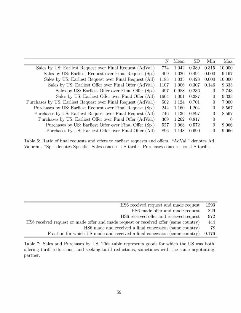
N Mean SD Min MaxSales by US: Earliest Request over Final Request (AdVal.) 774 1.042 0.389 0.315 10.000

Sales by US: Earliest Request over Final Request (Sp.) 409 1.020 0.494 0.000 9.167Sales by US: Earliest Request over Final Request (All) 1183 1.035 0.428 0.000 10.000Sales by US: Earliest Offer over Final Offer (AdVal.) 1107 1.006 0.307 0.146 9.333

Sales by US: Earliest Offer over Final Offer (Sp.) 497 0.988 0.236 0 2.743Sales by US: Earliest Offer over Final Offer (All) 1604 1.001 0.287 0 9.333

Purchases by US: Earliest Request over Final Request (AdVal.) 502 1.124 0.701 0 7.000Purchases by US: Earliest Request over Final Request (Sp.) 244 1.160 1.204 0 8.567Purchases by US: Earliest Request over Final Request (All) 746 1.136 0.897 0 8.567Purchases by US: Earliest Offer over Final Offer (AdVal.) 369 1.262 0.817 0 6

Purchases by US: Earliest Offer over Final Offer (Sp.) 527 1.068 0.572 0 9.066Purchases by US: Earliest Offer over Final Offer (All) 896 1.148 0.690 0 9.066

Table 6: Ratio of final requests and offers to earliest requests and offers. “AdVal.”denotes AdValorem. “Sp.”denotes Specific. Sales concern US tariffs. Purchases concern non-US tariffs.

HS6 received request and made request 1293HS6 made offer and made request 829

HS6 received offer and received request 972HS6 received request or made offer and made request or received offer (same country) 444

HS6 made and received a final concession (same country) 78Fraction for which US made and received a final concession (same country) 0.176

Table 7: Sales and Purchases by US. This table represents goods for which the US was bothoffering tariff reductions, and seeking tariff reductions, sometimes with the same negotiatingpartner.

59

Variable Obs Mean Std. Dev. Min MaxBy HS6 productN Suppliers to US 3064 10.539 11.321 1 118N Suppliers to US at Torquay 3064 6.507 5.536 0 36Torquay Volume Share 3064 0.772 0.31 0 1HHI of Suppliers (EXT) 3064 0.605 0.279 0.061 1Supply Absent from Torquay (ABSENT) 3064 0.228 0.31 0 1Undifferentiated (UNDIFF) 3064 0.322 0.467 0 1log(ω) 2694 .385 2.165 -5.63 7.134UK Preferences (PTA) 3064 0.531 0.499 0 1Requested Product (REQ) 3064 0.677 0.468 0 1Annecy Binding (PRVBND) 3064 0.125 0.331 0 1

By CountryTotal Volume 134 52420000 1.53E+08 15 1.55E+09Total Volume at Torquay 36 1.3E+08 2.68E+08 1562000 1.55E+09By HS6 product that US made an offer on or received a request for at TorquayTorquay Volume Share 2423 0.78 0.292 0 1HHI of Suppliers (EXT) 2423 0.577 0.271 0.061 1Supply Absent from Torquay (ABSENT) 2423 0.22 0.292 0 1Undifferentiated (UNDIFF) 2423 0.291 0.454 0 1log(ω) 2177 0.425 2.217 -5.63 7.134WANT (Offer Stage) 1636 3.106 8 0.746 107.167WANT (Failure Stage) 2423 2.259 6.62 0 92.5UK Preferences (PTA) 2423 0.529 0.499 0 1Requested Product (REQ) 2423 0.856 0.351 0 1Annecy Binding (PRVBND) 2423 0.131 0.338 0 1

Table 8: Trade Data Summary Statistics. log(ω) is the log inverse foreign export supplyelasticity as estimated by Broda, Limao, and Weinstein (2008) for the US at the HS4 level.

60

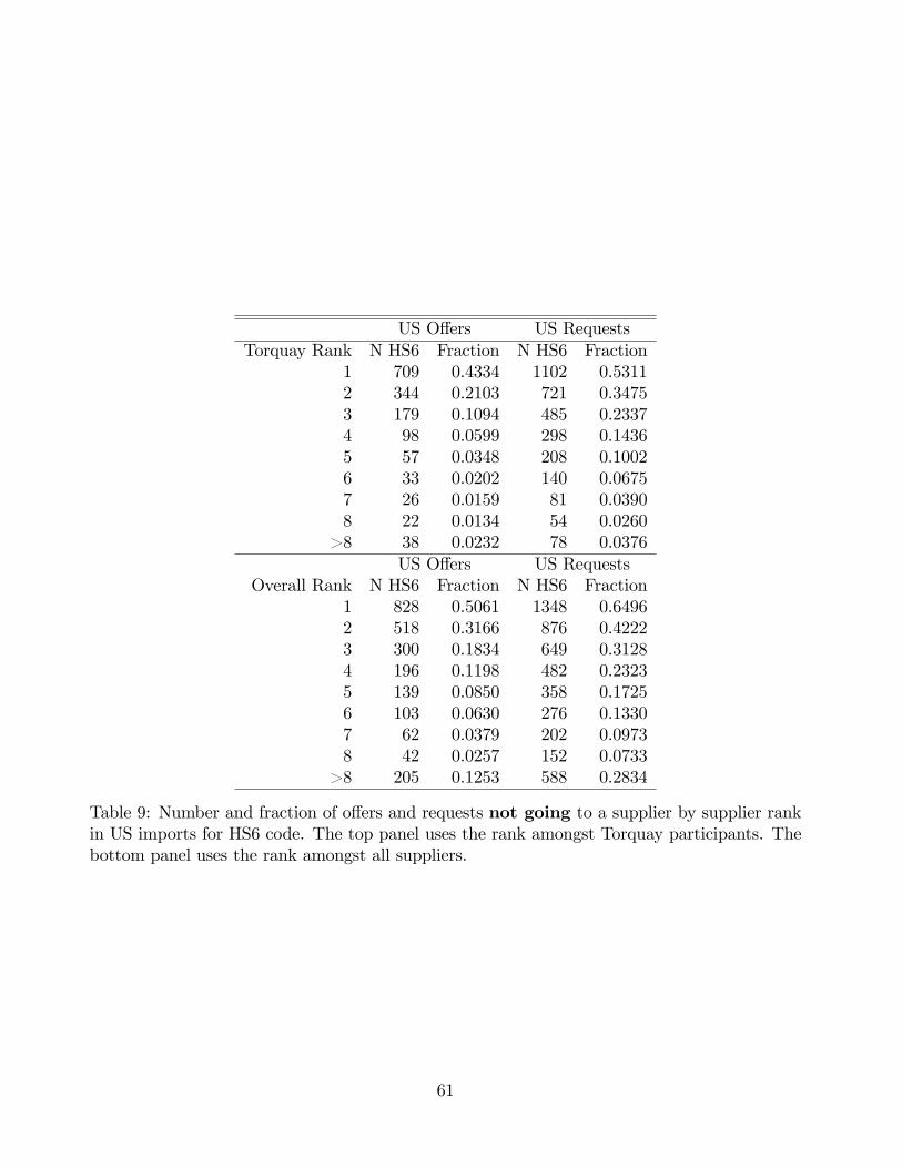
US Offers US RequestsTorquay Rank N HS6 Fraction N HS6 Fraction

1 709 0.4334 1102 0.53112 344 0.2103 721 0.34753 179 0.1094 485 0.23374 98 0.0599 298 0.14365 57 0.0348 208 0.10026 33 0.0202 140 0.06757 26 0.0159 81 0.03908 22 0.0134 54 0.0260

>8 38 0.0232 78 0.0376US Offers US Requests

Overall Rank N HS6 Fraction N HS6 Fraction1 828 0.5061 1348 0.64962 518 0.3166 876 0.42223 300 0.1834 649 0.31284 196 0.1198 482 0.23235 139 0.0850 358 0.17256 103 0.0630 276 0.13307 62 0.0379 202 0.09738 42 0.0257 152 0.0733

>8 205 0.1253 588 0.2834

Table 9: Number and fraction of offers and requests not going to a supplier by supplier rankin US imports for HS6 code. The top panel uses the rank amongst Torquay participants. Thebottom panel uses the rank amongst all suppliers.

61

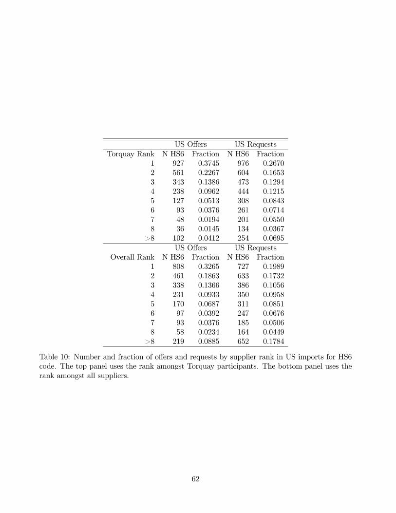
US Offers US RequestsTorquay Rank N HS6 Fraction N HS6 Fraction

1 927 0.3745 976 0.26702 561 0.2267 604 0.16533 343 0.1386 473 0.12944 238 0.0962 444 0.12155 127 0.0513 308 0.08436 93 0.0376 261 0.07147 48 0.0194 201 0.05508 36 0.0145 134 0.0367

>8 102 0.0412 254 0.0695US Offers US Requests

Overall Rank N HS6 Fraction N HS6 Fraction1 808 0.3265 727 0.19892 461 0.1863 633 0.17323 338 0.1366 386 0.10564 231 0.0933 350 0.09585 170 0.0687 311 0.08516 97 0.0392 247 0.06767 93 0.0376 185 0.05068 58 0.0234 164 0.0449

>8 219 0.0885 652 0.1784

Table 10: Number and fraction of offers and requests by supplier rank in US imports for HS6code. The top panel uses the rank amongst Torquay participants. The bottom panel uses therank amongst all suppliers.

62

OLS

OLS

Probit

Probit

OLS

OLS

Probit

Probit

USOffUKAUNZi

0.0623**

0.0700**

0.314*

0.485***

0.0564*

0.0666**

0.294*

0.449***

(0.0283)

(0.0282)

(0.168)

(0.147)

(0.0274)

(0.0271)

(0.161)

(0.136)

log(1+USImpi)

0.0122**

0.00690*

0.0591***

0.0475*

(0.00485)

(0.00347)

(0.0194)

(0.0258)

log(1+USImpi,f)

-0.0112**

-0.00899**

-0.0517***

-0.0594**

(0.00478)

(0.00355)

(0.0183)

(0.0237)

log(1+USImpUKAUNZi)

-0.00195

9.41e-05

-0.0113

-0.00299

(0.00295)

(0.00135)

(0.0154)

(0.0122)

Observations

1,815

1,815

1,815

1,668

1,815

1,815

1,815

1,668

R-squared

0.009

0.293

0.027

0.302

CountryFE

No

Yes

No

Yes

No

Yes

No

Yes

HS1FE

No

Yes

No

Yes

No

Yes

No

Yes

ClusterSE

Yes

Yes

Yes

Yes

Yes

Yes

Yes

Yes

Table11:RegressionofwhetheranHS6product-countrypairingofferedbytheUSwasaddedafter2/18/1951(afterthe

breakdownofUSandUKbilateralnegotiation)onwhethertheproductinquestionwasofferedbytheUStotheUK.A

positivecoefficientimpliesthataproductismorelikelytobeofferedbytheUSfollowingtheUS-UKbilateralbreakdown

iftheUSwasofferingaconcessiononthisproducttotheUKbeforethenegotiationfailure.SE’sclusteredbynegotiating

partner.

63

Offer Failure Failure Failure Offer Failure Failure FailureProbit OLS OLS OLS Probit OLS OLS OLS

EXT 0.736 0.990*** 1.100*** 0.844*** 0.783 0.831*** 0.990*** 0.635**(0.490) (0.238) (0.268) (0.244) (0.529) (0.252) (0.280) (0.258)

EXT2 -0.944** -0.615*** -0.751*** -0.533*** -1.007** -0.466** -0.665*** -0.335(0.381) (0.186) (0.240) (0.194) (0.409) (0.197) (0.249) (0.205)

WANT 0.0112*** -0.00252* -0.00193 -0.00175 0.0133*** -0.00244* -0.00145 -0.00210(0.00431) (0.00136) (0.00151) (0.00139) (0.00474) (0.00148) (0.00166) (0.00152)

ABSENT -0.192** 0.0922** 0.0649 0.0826* -0.168 0.0985** 0.0649 0.0849*(0.0963) (0.0465) (0.0555) (0.0481) (0.103) (0.0488) (0.0553) (0.0506)

PTA 0.313*** 0.0822*** 0.124** 0.0610** 0.356*** 0.0712*** 0.136** 0.0364(0.0593) (0.0259) (0.0530) (0.0268) (0.0635) (0.0275) (0.0567) (0.0290)

REQ 0.572*** 0.0126 0.102 0.524*** 0.0367 0.148(0.0546) (0.0267) (0.102) (0.0595) (0.0288) (0.0908)

PrevBound 0.217*** -0.0720** -0.0442 -0.0838** 0.209*** -0.0574* -0.0212 -0.0842**(0.0748) (0.0316) (0.0442) (0.0327) (0.0804) (0.0339) (0.0439) (0.0352)

UNDIFF 0.0519 -0.105*** -0.0980*** -0.118*** 0.0633 -0.124*** -0.112*** -0.152***(0.0614) (0.0278) (0.0289) (0.0246) (0.0670) (0.0303) (0.0316) (0.0269)

log(ω) 0.0539*** -0.0123** -0.00278 -0.0271***(0.0130) (0.00551) (0.00917) (0.00554)

λ̂ 0.238 -0.00175 0.327 -0.00210(0.264) (0.00139) (0.252) (0.00152)

Obs 3,064 1,636 1,636 1,636 2,694 1,456 1,456 1,456R-squared 0.109 0.109 0.041 0.127 0.128 0.054HS1 FE Y Y Y Y Y Y

Table 12: Offer and failure equations conditional on theoretical predictors. Columns 1 and 5correspond to the offer equation, estimated as a Probit. Columns 2-4 and 6-8 correspond tofailure equations. Columns 2 and 6 do not make any selection correction. Columns 3 and 7use the inverse Mills ratio from the offer equation, but no excluded variables. Columns 4 and 8exclude REQ and HS1 fixed effects from the failure equation. Columns 1-4 omit ω, the marketpower measure as it is not available for all products. WANT is defined with respect to theprincipal supplier in the offer regression, whereas it is defined with respect to the highest USimport volume (for the good in question) country who received the offer in the failure regression

64