Multilevel Methods forEigenspace Computations in

Structural Dynamics

Ulrich Hetmaniuk & Rich LehoucqSandia National Laboratories,

Computational Math and Algorithms,Albuquerque, NM

Joint work with Peter Arbenz (ETH), Jeff Bennighof (UT Austin), MarkMuller (UT Austin), Bill Cochran (UIUC), Heidi Thornquist & Ray

Tuminaro (Sandia)

Eigenvalue problem instructural dynamics

• Who/What is the problem?• Multilevel approach 1 (use multilevel

preconditioners)• Multilevel approach 2 (component

mode synthesis)• Conclusions and future directionsThanks to the organizers

Eigen-gang

Jeff Bennighof,University of Texas

Mark Muller,University of Texas(Jeff’s Ph.D student)

Bill Cochran, Sandiasummer intern; Ph.d.student UIUC

Peter Arbenz, ETH

Ray Tuminaro,Sandia Heidi Thornquist

Sandia

Ulrich Hetmaniuk,Sandia

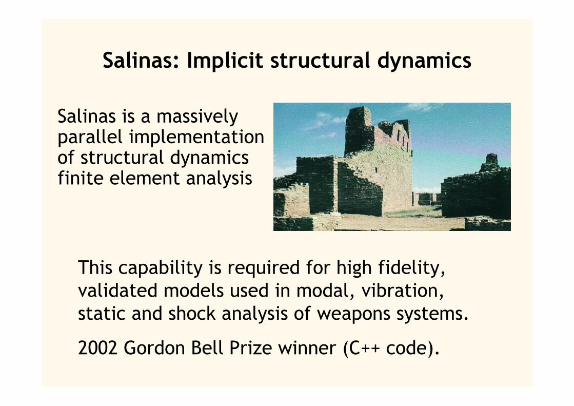
Salinas: Implicit structural dynamics

Salinas is a massivelyparallel implementationof structural dynamicsfinite element analysis

This capability is required for high fidelity,validated models used in modal, vibration,static and shock analysis of weapons systems.

2002 Gordon Bell Prize winner (C++ code).

Salinas and linear algebra

Robust scalable iterative linear and eigensolversare required

Fundamental mode of an aircraft carrier

Assume that appropriate initial and boundaryconditions are specified and that is a two orthree dimensional domain that represents astructure.

Consider the hyperbolic PDE on a domain

PDE of interest

where is a linear elliptic coerciveoperator and is the mass density.

( )uE

( ) ( )ttu u f tρ − =E

ρ

Ω

Ω

Problems of interest

• Frequency (or harmonic) response—how does the structure respond to aprescribed load?

• Transient analysis—how does thestructure evolve in time?

My assumption is that 100 plus eigenpairsare needed for large-scale 3D FEMdiscretizations—the eigenpairs effect areduced order model (ROM).

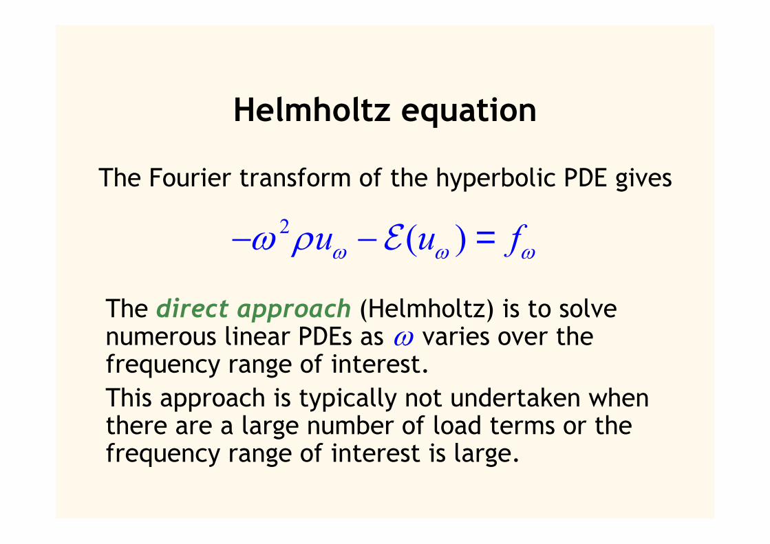
Helmholtz equation

The direct approach (Helmholtz) is to solvenumerous linear PDEs as varies over thefrequency range of interest.This approach is typically not undertaken whenthere are a large number of load terms or thefrequency range of interest is large.

ω

The Fourier transform of the hyperbolic PDE gives

2 ( )u u fω ω ωω ρ− − =E

• This standard approach computes numerousmodes and then projects the PDE onto themodal subspace.

• This approach is useful when there are manyload terms or the frequency range of interestis large.

over the domain with the same boundaryconditions as the ROM.

( )i i iz zλ ρ− =EΩ

Compute the free vibrations or modal subspaceof

Modal approach (ROM)

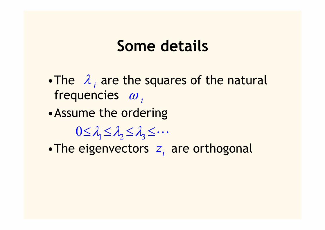
Some details

•The are the squares of the naturalfrequencies

•Assume the ordering

•The eigenvectors are orthogonal

iλiω

iz1 2 30 λ λ λ≤ ≤ ≤ ≤

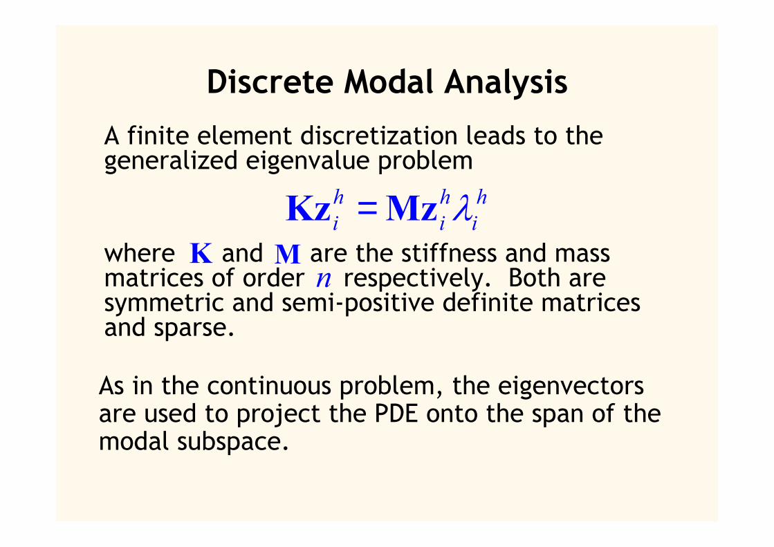
A finite element discretization leads to thegeneralized eigenvalue problem

where and are the stiffness and massmatrices of order respectively. Both aresymmetric and semi-positive definite matricesand sparse.

Discrete Modal Analysis

As in the continuous problem, the eigenvectorsare used to project the PDE onto the span of themodal subspace.

h h hi i iλ=Kz Mz

K Mn

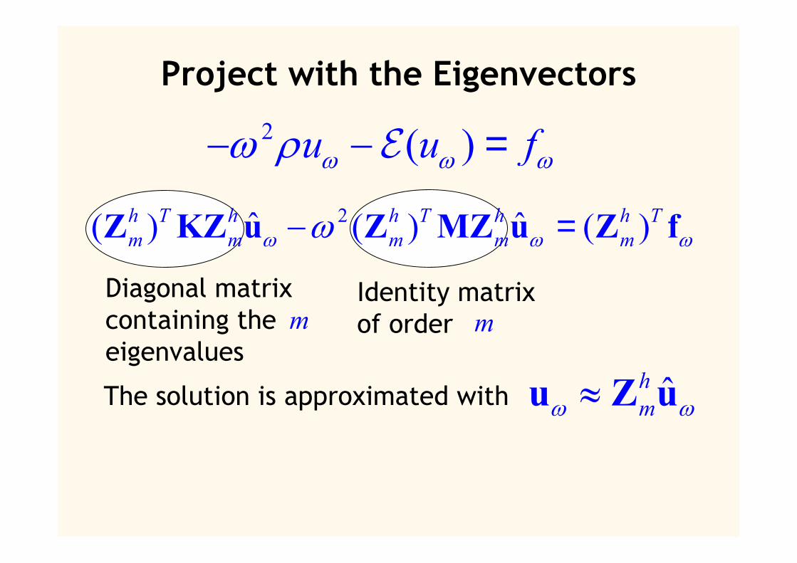
Project with the Eigenvectors

The solution is approximated with ˆhmω ω≈u Z u

Identity matrixof order mm

Diagonal matrixcontaining theeigenvalues

2ˆ ˆ( ) ( ) ( )h T h h T h h Tm m m m mω ω ωω− =Z KZ u Z MZ u Z f

2 ( )u u fω ω ωω ρ− − =E

Why only modes?• Eigenvectors associated with the smallest

eigenvalues have a mechanical significance—they dominate the low–frequency response

• FEM discretization only approximates a smallnumber of fundamental modes of the PDE—why compute more? (Error increases as thefrequency increases)

• Keep in mind that thousands of eigenvectorsmay be needed when the modal density islarge—many eigenvalues within the desiredfrequency range.

m

Eigenvalue problem instructural dynamics

• Who/What is the problem?• Multilevel approach 1 (use multilevel

preconditioners)• Multilevel approach 2 (component

mode synthesis)• Conclusions and future directions

Requirements of an algorithmand ensuing implementation

• Robust (vary data, parameters and stillcompute the same answers)

• Reliable (don’t miss eigenvalues,compute a basis of eigenvectors)

• Return orthogonal eigenvectors• Ability to efficiently compute 100-

10,000 modes (remember we togenerate a ROM).

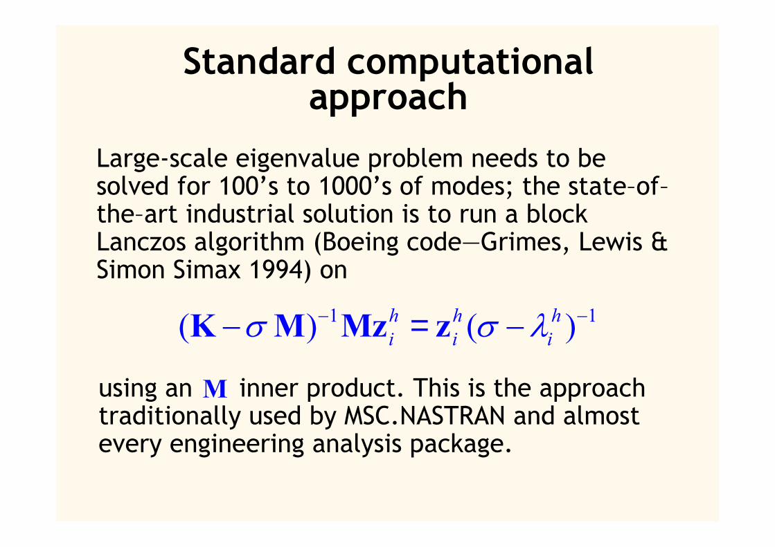
Standard computationalapproach

Large-scale eigenvalue problem needs to besolved for 100’s to 1000’s of modes; the state–of–the–art industrial solution is to run a blockLanczos algorithm (Boeing code—Grimes, Lewis &Simon Simax 1994) on

using an inner product. This is the approachtraditionally used by MSC.NASTRAN and almostevery engineering analysis package.

1 1( ) ( )h h hi i iσ σ λ− −− = −K M Mz z

Μ

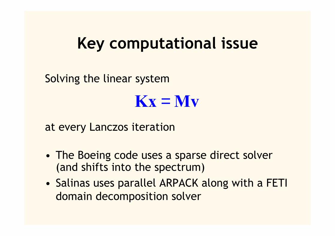
Key computational issue

Solving the linear system

=Kx Mvat every Lanczos iteration

• The Boeing code uses a sparse direct solver(and shifts into the spectrum)

• Salinas uses parallel ARPACK along with a FETIdomain decomposition solver

Overview of multilevel approach 1

1. Shift-invert Lanczos method with ascalable preconditioned inneriteration

2. Preconditioned eigensolver (no inneriteration necessary)

h h hi i iλ=Kz Mz

1( , ) Span , , , mmK

−=

≡ -1

T x x Tx T x

T K M

Shift-invert Lanczos with apreconditioned inner iteration

Apply via a preconditionedconjugate iteration—use ascalable preconditioner(multilevel/multigrid)

Preconditioned Eigensolver

Only require an application of a preconditionerper (outer) iteration

(0) (0) ( ) 1 ( ) ( )1

( ) ( )( ) ( )

( ) ( )

( ) Span , , , ( )

( )and( )min

m

m m mm

m mm m

m mD

D θ

θ

−+

∈

= −

= ≡T T

T Tx

x x x N M K x

x Kx x Kxxx Mx x Mx

N

Preconditioned Eigensolver

Replace shift-invert Lanczos—attempt tominimize the Rayleigh-Quotient

• Newton’s method (Davidson methods)(Davidson, Morgan, Scott, van der Vorst,Sleijpen, Stathopoulos, Saad, Notay)

• Nonlinear conjugate gradient iteration(Longsine, McCormick, Knyazev,Bergamaschi, Pini)

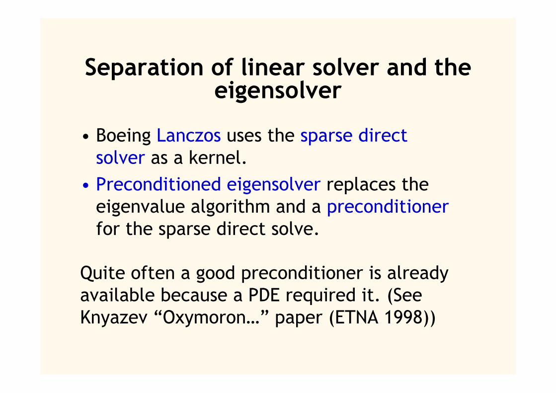
Separation of linear solver and theeigensolver

• Boeing Lanczos uses the sparse directsolver as a kernel.

• Preconditioned eigensolver replaces theeigenvalue algorithm and a preconditionerfor the sparse direct solve.

Quite often a good preconditioner is alreadyavailable because a PDE required it. (SeeKnyazev “Oxymoron…” paper (ETNA 1998))

Repeated use of stiffness, mass matrices andrepeated preconditioning of the large-scaleproblem and cost of maintainingorthogonality.

Clearly not an issue for a small number ofmodes or a limited frequency response (smallfrequency range).

What about a large number of eigenvectors?

Potential limitations of thesemethods

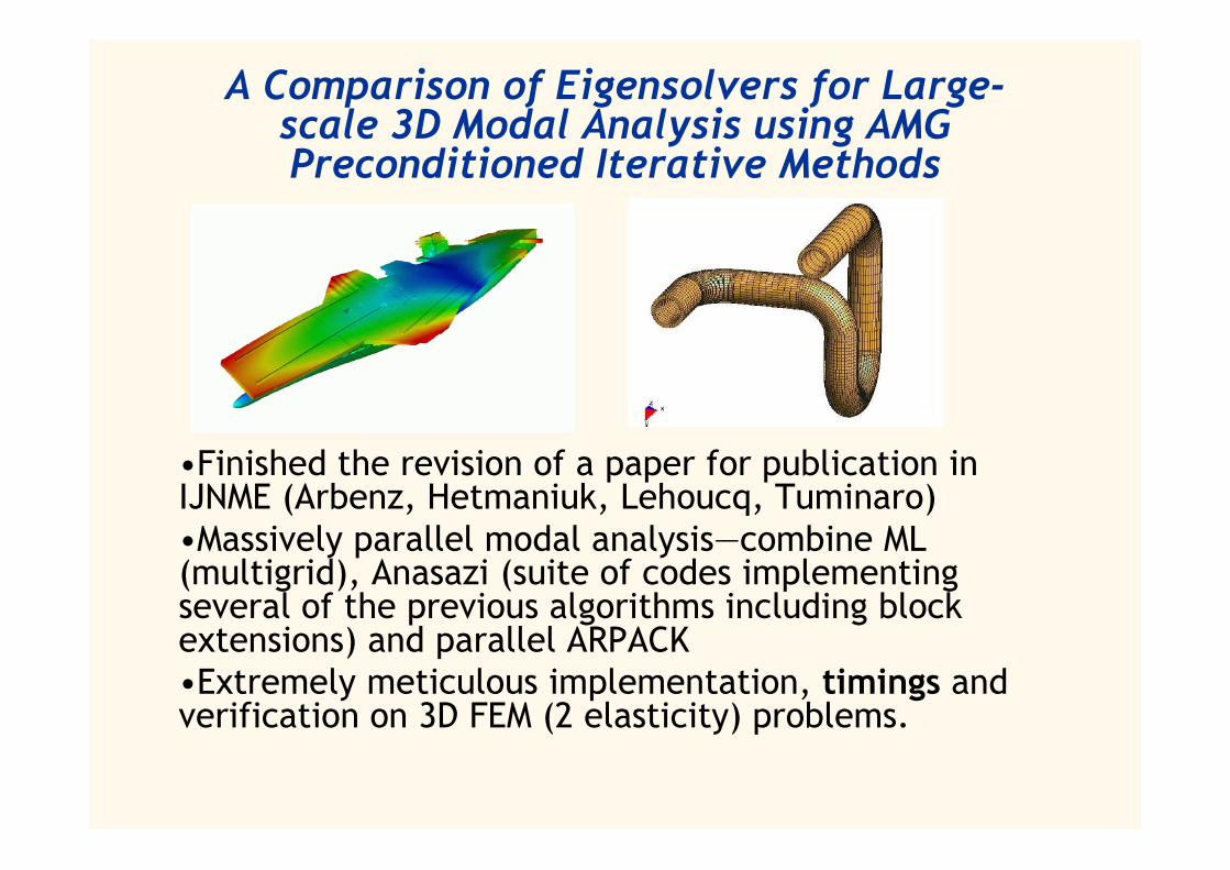
A Comparison of Eigensolvers for Large-scale 3D Modal Analysis using AMGPreconditioned Iterative Methods

•Finished the revision of a paper for publication inIJNME (Arbenz, Hetmaniuk, Lehoucq, Tuminaro)•Massively parallel modal analysis—combine ML(multigrid), Anasazi (suite of codes implementingseveral of the previous algorithms including blockextensions) and parallel ARPACK•Extremely meticulous implementation, timings andverification on 3D FEM (2 elasticity) problems.

One conclusion from ourcomparison

The cost of all the algorithms isasymptotic with the cost of maintainingorthogonality of the eigenvectors as thenumber of eigenpairs requested isincreased.

Are there alternate approaches?

Eigenvalue problem instructural dynamics

• Who/What is the problem?• Multilevel approach 1 (use multilevel

preconditioners)• Multilevel approach 2 (component

mode synthesis ideas)• Conclusions and future directions

Component Mode Synthesis

Component Mode Synthesis (CMS) techniquesoriginated in the aerospace engineeringcommunity (Hurty 1965, Craig-Bampton 1968).The idea is simple.

1. Decompose the structure into componentparts

2. Determine the modes of the parts

3. Synthesize these component modes to saysomething about the structure

Matrix view of CMSOne way dissection on the union of the graphs ofthe mass and stiffness matrices produces

1 1

2 2

1 2

,

,

, ,

T

T

Ω Γ Ω

Ω Γ Ω

Γ Ω Γ Ω Γ

K 0 K

0 K K

K K Kand

1 1

2 2

1 2

,

,

, ,

T

T

Ω Γ Ω

Ω Γ Ω

Γ Ω Γ Ω Γ

M 0 M

0 M M

M M M

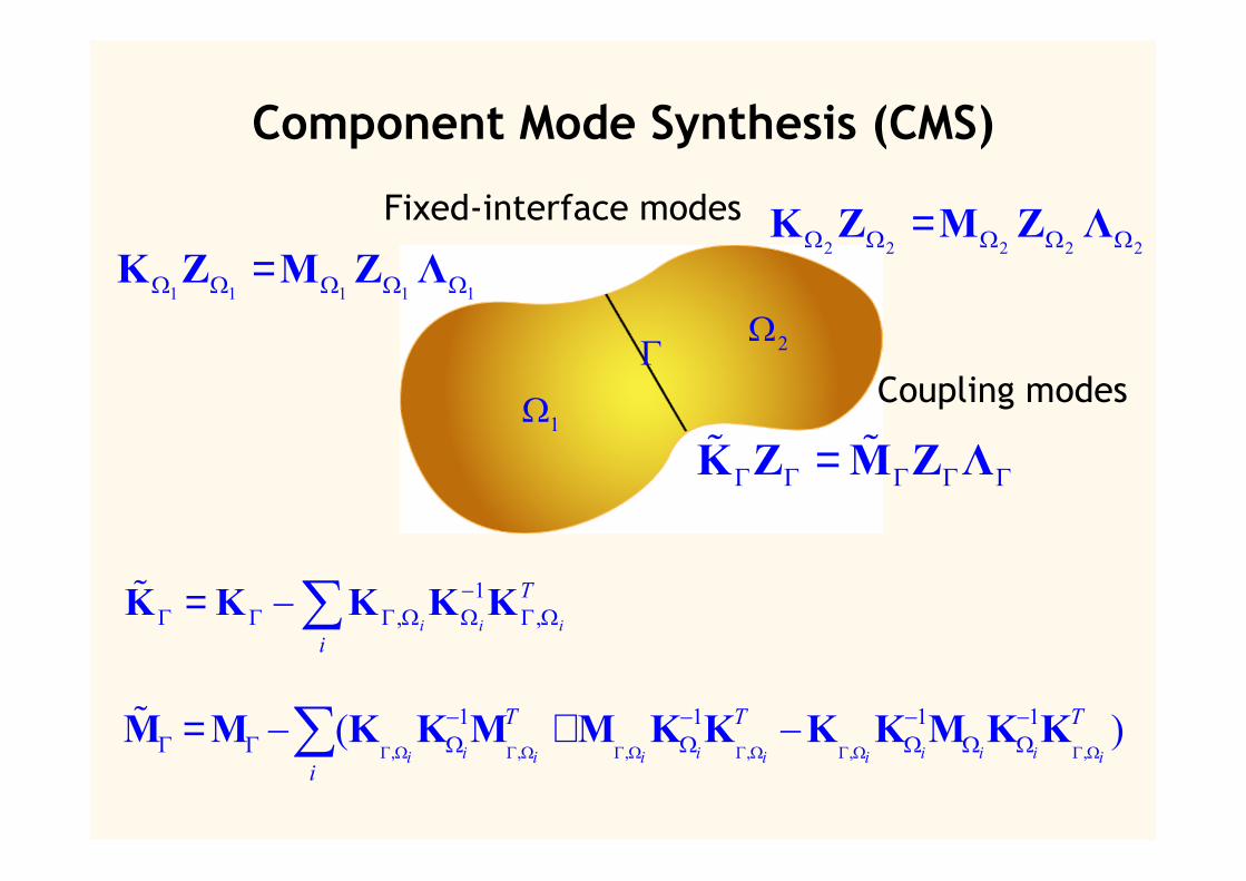
Component Mode Synthesis (CMS)

1Ω

2ΩΓ

1 1 1 1 1Ω Ω Ω Ω Ω=K Z M Z Λ2 2 2 2 2Ω Ω Ω Ω Ω=K Z M Z ΛFixed-interface modes

Γ Γ Γ Γ Γ=K Z M Z Λ Coupling modes

1, ,i i i

T

i

−Γ Γ Γ Ω Ω Γ Ω= −∑K K K K K

, , , , , ,

1 1 1 1( )i i i i ii i i i i i

T T T

iΓ Ω Γ Ω Γ Ω Γ Ω Γ Ω Γ Ω

− − − −Γ Γ Ω Ω Ω Ω Ω= − + −∑M M K K M M K K K K M K K

TheoremThe interface eigenvalue problem is equivalent to:Find such that

where the Steklov-Poincaré and mass operatorsact on

1/ 200( , ) ( )u Hλ ∈ Γ ×ℜ

1/200, , ( )Su v Mu v v Hλ= ∀ ∈ Γ

&S M1/ 200 ( ) :Hτ ∈ Γ

2

1

( ( ) )i ii

S Eτ σ τ η Γ=

= ⋅∑2

1

( ( ( )) )i i ii

M G Eτ σ ρ τ η Γ=

= ⋅∑

iEis the Green’s function for the Dirichlet problem

on and extends a trace function to .( )iG ⋅

iΩ iΩ

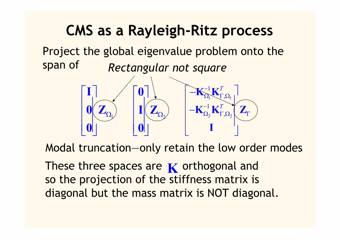
CMS as a Rayleigh-Ritz process

Rectangular not square

1Ω

I0 Z0

1 1

2 2

1,

1,

T

T

−Ω Γ Ω

−Ω Γ Ω Γ

− −

K K

K K Z

I2Ω

0I Z0

Project the global eigenvalue problem onto thespan of

These three spaces are orthogonal andso the projection of the stiffness matrix isdiagonal but the mass matrix is NOT diagonal.

KModal truncation—only retain the low order modes

Previous/related work

• Bourquin (1992, 1993) casts CMS in avariational setting

• Asymptotic error analysis for 1,2,3dimensional elliptic equations and theirdiscretization

• Error is sum of modal truncation anddiscretization errors

• Can also consider free-interface methods(introduce a Lagrange multiplier at theinterface)

AMLS

Ω1,1

Ω1,2

Γ0,1

Ω2,1

Ω2,2

Ω2,3

Ω2,4

Ω2,5Γ1,2Γ0,1

Γ1,1

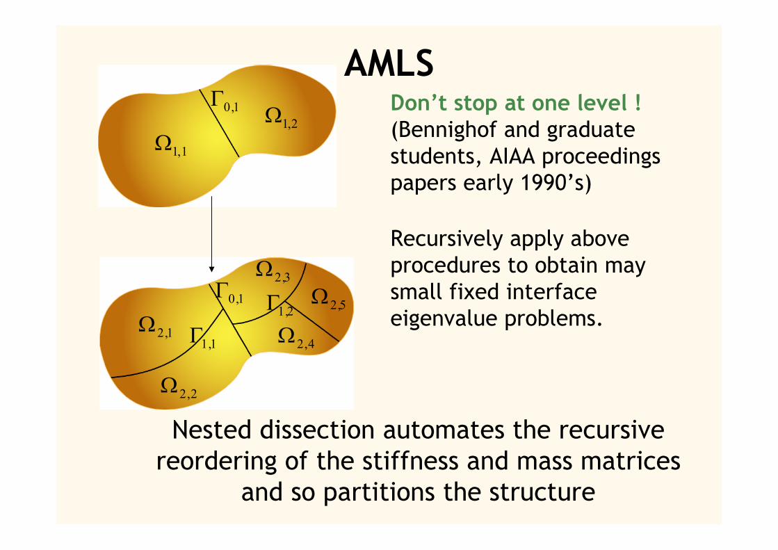
Don’t stop at one level !(Bennighof and graduatestudents, AIAA proceedingspapers early 1990’s)

Recursively apply aboveprocedures to obtain maysmall fixed interfaceeigenvalue problems.

Nested dissection automates the recursivereordering of the stiffness and mass matrices

and so partitions the structure

ReferenceAn Automated Multilevel SubstructuringMethod for Eigenspace Computation in LinearElastodynamics SISC, 2004, by Bennighof & L.

• AMLS cast in a multilevel variational formulation(extension of the work by Bourquin)

• Showed that discrete AMLS represents a matrixdecomposition of the stiffness matrix. The resultingdecomposition performs a change of coordinates

• AMLS is a Rayleigh-Ritz method that efficientlycomputes an approximation to the modal subspace—reduced order modeling

Example AMLS Calculation

• Recent paper Efficient Broadband Vibro-Acoustic Analysis of Passenger Car bodiesUsing an FE-based Component ModeSynthesis approach (Kropp & Heiserer,proceedings of the World Congress inComputational Mechanics, Vienna, 2002).

• Compared the industry standard BlockLanczos as (embedded in MSC.Nastran)approach against AMLS on modal analysis onthe BMW 3 series.

BMW comparison result

AMLSDirect(Helmholtz)

Boeing Lanczos

DOFS (Matrix order) mesh refinement510 610 710

Freq

uenc

yra

nge

(Hz)

100

1600

Cost of the computations• These computations were performed on an

HP 9000 (800 MHz) with 2 gigabytes ofmemory.

• The largest calculation took just under 3days (2,500 eigenvectors for a problem with13.5 million DOFs!).

• A 2.3 million DOF computation up through400 Hz took 4 days of cputime and over aweek turnaround time on a CRAY SV1 usingthe block Lanczos code. This calculation isnot even feasible on the HP 9000.

Some stats on the BMW problemOrder 13.5 million problem substructured into

• 38 levels• 46,767 substructures• Order 37,848 coarse problem

During the past three years, AMLS hasreplaced Boeing Lanczos within theautomotive industry. Craysupercomputers have been replaced byPC/workstations

Limitations of AMLS

Not a good technique for 3D problems becauseof the size of the interface eigenvalueproblem.

AMLS assumes that the interface matrixoperators are formed and factored.

Important to point out that AMLS has the samecomplexity of one sparse direct factorizationof the stiffness matrix.

Mass interface operator

How can we approximate the abovematrix operator? It’s expensive to applybecause of the amount of data.

, , , , , ,

1 1 1 1( )i i i i ii i i i i i

T T T

iΓ Ω Γ Ω Γ Ω Γ Ω Γ Ω Γ Ω

− − − −Γ Γ Ω Ω Ω Ω Ω= − + −∑M M K K M M K K K K M K K

Multilevel approach 2 alternatives

• CMS technique where the interfaceoperators are not formed and insteadpreconditioned eigensolvers areemployed.– For example, use the BDDC (Dohrmann)

preconditioner at the interface. Problem:Multilevel approach 1 issues come to bear.

• Algebraic multilevel?

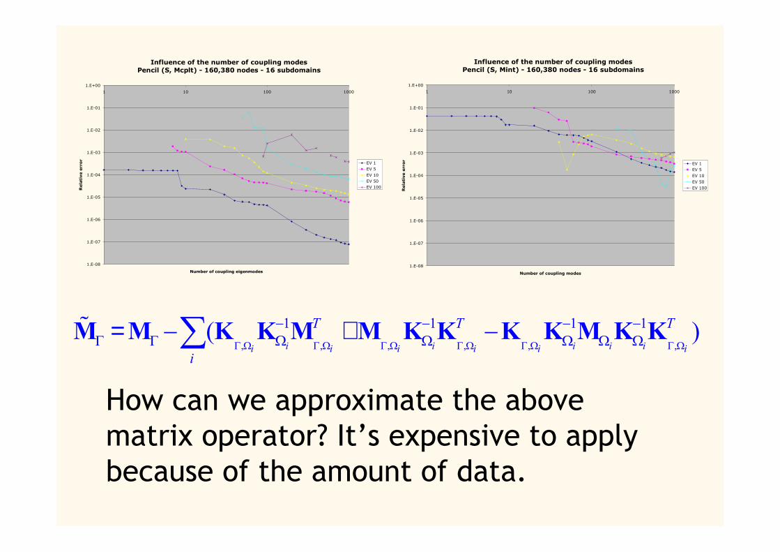
Influence of the number of coupling modesPencil (S, Mcplt) - 160,380 nodes - 16 subdomains

1.E-08

1.E-07

1.E-06

1.E-05

1.E-04

1.E-03

1.E-02

1.E-01

1.E+00

1 10 100 1000

Number of coupling eigenmodes

Rela

tive e

rro

r

EV 1EV 5

EV 10EV 50EV 100

Influence of the number of coupling modesPencil (S, Mint) - 160,380 nodes - 16 subdomains

1.E-08

1.E-07

1.E-06

1.E-05

1.E-04

1.E-03

1.E-02

1.E-01

1.E+00

1 10 100 1000

Number of coupling modes

Rela

tive e

rror

EV 1EV 5

EV 10

EV 50

EV 100

, , , , , ,

1 1 1 1( )i i i i ii i i i i i

T T T

iΓ Ω Γ Ω Γ Ω Γ Ω Γ Ω Γ Ω

− − − −Γ Γ Ω Ω Ω Ω Ω= − + −∑M M K K M M K K K K M K K

How can we approximate the abovematrix operator? It’s expensive to applybecause of the amount of data.

Algebraic Multilevel

• Start with RQMG (Mandel and McCormick1989) that approximately minimizes theRayleigh Quotient over a sequence of grids.

• We’re replacing the geometric informationand smoothers of RQMG with algebraic infoand better smoothers resulting in RQAMG.

Goal of RQAMG is to overcome the cost ofmaintaining numerical orthogonality of the Ritzvectors associated with multilevel approach 1.Work in progress, Hetmaniuk & L.

Summary of multilevel approaches

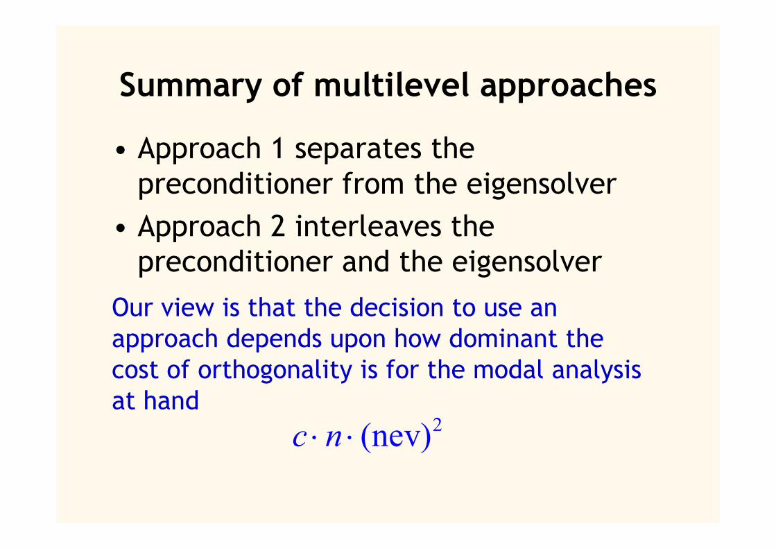
• Approach 1 separates thepreconditioner from the eigensolver

• Approach 2 interleaves thepreconditioner and the eigensolver

Our view is that the decision to use anapproach depends upon how dominant thecost of orthogonality is for the modal analysisat hand

2(nev)c n⋅ ⋅

Future/ongoing work

• Error estimation and stopping criterion (joint workwith Hetmaniuk, Knyazev and Ovtchinnikov) formultilevel aproach 1

• Modal truncation criterion (recent reports by others)• Regularity issues or the effect of partitions on the

approximation of global modes• Approximation of the mass interface operator• RQAMG, preconditioned CMS• Packaging the preconditioned eigensolvers for public

release into a the Anasazi subpackage of Trilinos(joint with Hetmaniuk and Thornquist)

• DD16 proceedings paper