multinomial logit models
TRANSCRIPT
Multinomial Logit Models
Akshita, Ramyani, Sridevi & Trishita
Econometrics-II, Instructor : Dr. Subrata Sarkar, IGIDR
19 April 2013
Group 7 Multinomial Logit Models
INTRODUCTION
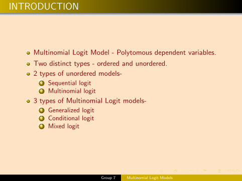
Multinomial Logit Model - Polytomous dependent variables.
Two distinct types - ordered and unordered.
2 types of unordered models-1 Sequential logit2 Multinomial logit
3 types of Multinomial Logit models-1 Generalized logit2 Conditional logit3 Mixed logit
Group 7 Multinomial Logit Models
INTRODUCTION
Multinomial Logit Model - Polytomous dependent variables.
Two distinct types - ordered and unordered.
2 types of unordered models-1 Sequential logit2 Multinomial logit
3 types of Multinomial Logit models-1 Generalized logit2 Conditional logit3 Mixed logit
Group 7 Multinomial Logit Models
ASSUMPTIONS
Data are case specific.
Independence among the choices of dependent variable.
Errors are independently and identically distributed.
Group 7 Multinomial Logit Models
ASSUMPTIONS
Data are case specific.
Independence among the choices of dependent variable.
Errors are independently and identically distributed.
Group 7 Multinomial Logit Models
ASSUMPTIONS
Data are case specific.
Independence among the choices of dependent variable.
Errors are independently and identically distributed.
Group 7 Multinomial Logit Models
THEORETICAL FRAMEWORK
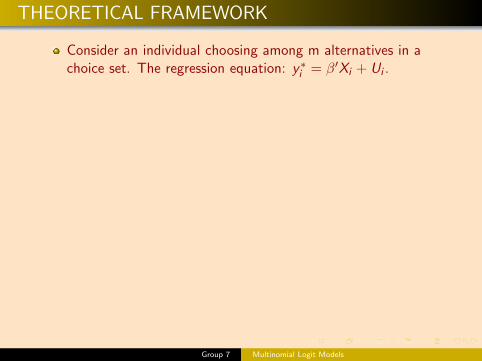
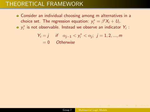
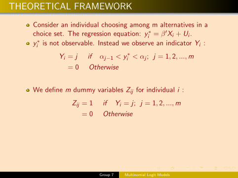
Consider an individual choosing among m alternatives in achoice set. The regression equation: y∗i = β′Xi + Ui .
y∗i is not observable. Instead we observe an indicator Yi :
Yi = j if αj−1 < y∗i < αj ; j = 1, 2, ...,m
= 0 Otherwise
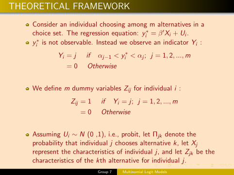
We define m dummy variables Zij for individual i :
Zij = 1 if Yi = j ; j = 1, 2, ...,m
= 0 Otherwise
Assuming Ui ∼ N (0 ,1), i.e., probit, let Πjk denote theprobability that individual j chooses alternative k, let Xj
represent the characteristics of individual j , and let Zjk be thecharacteristics of the kth alternative for individual j .
Group 7 Multinomial Logit Models
THEORETICAL FRAMEWORK
Consider an individual choosing among m alternatives in achoice set. The regression equation: y∗i = β′Xi + Ui .
y∗i is not observable. Instead we observe an indicator Yi :
Yi = j if αj−1 < y∗i < αj ; j = 1, 2, ...,m
= 0 Otherwise
We define m dummy variables Zij for individual i :
Zij = 1 if Yi = j ; j = 1, 2, ...,m
= 0 Otherwise
Assuming Ui ∼ N (0 ,1), i.e., probit, let Πjk denote theprobability that individual j chooses alternative k, let Xj
represent the characteristics of individual j , and let Zjk be thecharacteristics of the kth alternative for individual j .
Group 7 Multinomial Logit Models
GENERALIZED LOGIT MODELS
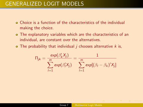
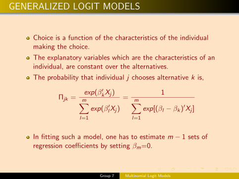
Choice is a function of the characteristics of the individualmaking the choice.
The explanatory variables which are the characteristics of anindividual, are constant over the alternatives.
The probability that individual j chooses alternative k is,
Πjk =exp(β′kXj)m∑l=1
exp(β′lXj)
=1
m∑l=1
exp[(βl − βk)′Xj ]
In fitting such a model, one has to estimate m − 1 sets ofregression coefficients by setting βm=0.
Group 7 Multinomial Logit Models
GENERALIZED LOGIT MODELS
Choice is a function of the characteristics of the individualmaking the choice.
The explanatory variables which are the characteristics of anindividual, are constant over the alternatives.
The probability that individual j chooses alternative k is,
Πjk =exp(β′kXj)m∑l=1
exp(β′lXj)
=1
m∑l=1
exp[(βl − βk)′Xj ]
In fitting such a model, one has to estimate m − 1 sets ofregression coefficients by setting βm=0.
Group 7 Multinomial Logit Models
CONDITIONAL LOGIT MODELS
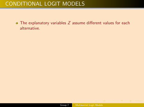
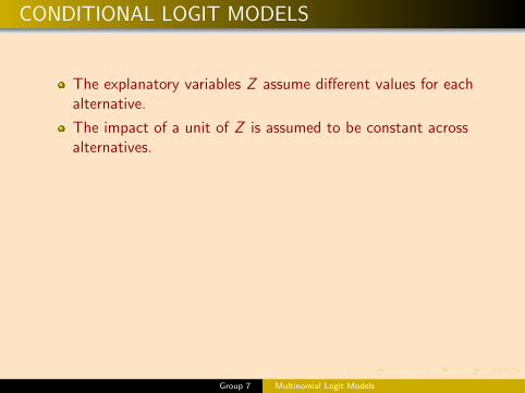
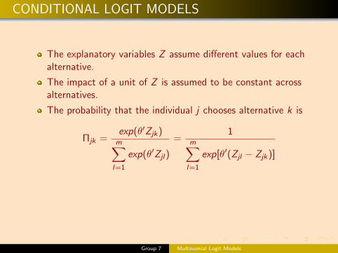
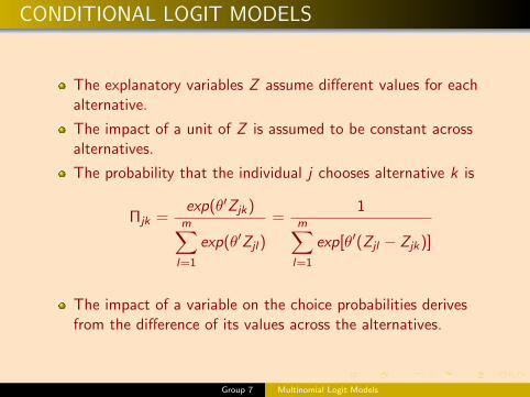
The explanatory variables Z assume different values for eachalternative.
The impact of a unit of Z is assumed to be constant acrossalternatives.
The probability that the individual j chooses alternative k is
Πjk =exp(θ′Zjk)m∑l=1
exp(θ′Zjl)
=1
m∑l=1
exp[θ′(Zjl − Zjk)]
The impact of a variable on the choice probabilities derivesfrom the difference of its values across the alternatives.
Group 7 Multinomial Logit Models
CONDITIONAL LOGIT MODELS
The explanatory variables Z assume different values for eachalternative.
The impact of a unit of Z is assumed to be constant acrossalternatives.
The probability that the individual j chooses alternative k is
Πjk =exp(θ′Zjk)m∑l=1
exp(θ′Zjl)
=1
m∑l=1
exp[θ′(Zjl − Zjk)]
The impact of a variable on the choice probabilities derivesfrom the difference of its values across the alternatives.
Group 7 Multinomial Logit Models
MIXED LOGIT MODELS
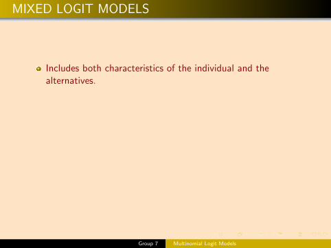
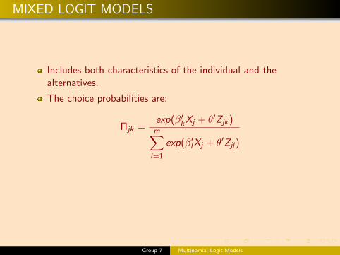
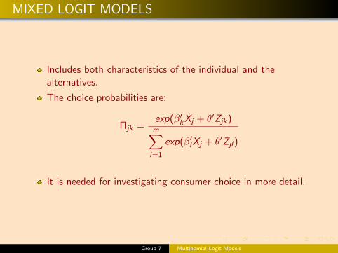
Includes both characteristics of the individual and thealternatives.
The choice probabilities are:
Πjk =exp(β′kXj + θ′Zjk)m∑l=1
exp(β′lXj + θ′Zjl)
It is needed for investigating consumer choice in more detail.
Group 7 Multinomial Logit Models
MIXED LOGIT MODELS
Includes both characteristics of the individual and thealternatives.
The choice probabilities are:
Πjk =exp(β′kXj + θ′Zjk)m∑l=1
exp(β′lXj + θ′Zjl)
It is needed for investigating consumer choice in more detail.
Group 7 Multinomial Logit Models
MIXED LOGIT MODELS
Includes both characteristics of the individual and thealternatives.
The choice probabilities are:
Πjk =exp(β′kXj + θ′Zjk)m∑l=1
exp(β′lXj + θ′Zjl)
It is needed for investigating consumer choice in more detail.
Group 7 Multinomial Logit Models
MIXED LOGIT MODEL AS GENERALIZED LOGITMODEL
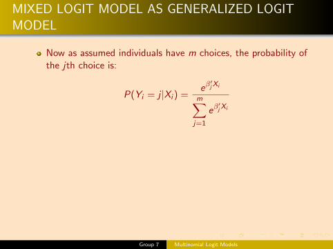
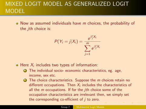
Now as assumed individuals have m choices, the probability ofthe jth choice is:
P(Yi = j |Xi ) =eβ′jXi
m∑j=1
eβ′jXi
Here Xi includes two types of information:1 The individual socio- economic characteristics, eg. age,
income, sex etc.2 The choice characteristics. Suppose the m choices retain no
different occupations. Then Xi includes the characteristics ofall the m occupations. If for the jth choice some of theoccupation characteristics are irrelevant then, we simply setthe corresponding co-efficient of j to zero.
Group 7 Multinomial Logit Models
MIXED LOGIT MODEL AS GENERALIZED LOGITMODEL
Now as assumed individuals have m choices, the probability ofthe jth choice is:
P(Yi = j |Xi ) =eβ′jXi
m∑j=1
eβ′jXi
Here Xi includes two types of information:1 The individual socio- economic characteristics, eg. age,
income, sex etc.2 The choice characteristics. Suppose the m choices retain no
different occupations. Then Xi includes the characteristics ofall the m occupations. If for the jth choice some of theoccupation characteristics are irrelevant then, we simply setthe corresponding co-efficient of j to zero.
Group 7 Multinomial Logit Models
Continued...
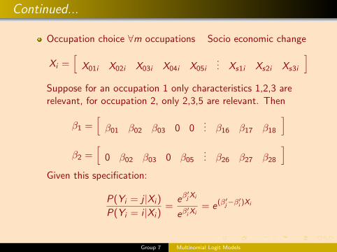
Occupation choice ∀m occupations Socio economic change
Xi =[X01i X02i X03i X04i X05i
... Xs1i Xs2i Xs3i
]Suppose for an occupation 1 only characteristics 1,2,3 arerelevant, for occupation 2, only 2,3,5 are relevant. Then
β1 =[β01 β02 β03 0 0
... β16 β17 β18
]β2 =
[0 β02 β03 0 β05
... β26 β27 β28
]Given this specification:
P(Yi = j |Xi )
P(Yi = i |Xi )=
eβ′jXi
eβ′iXi
= e(β′j−β
′i )Xi
Group 7 Multinomial Logit Models
Continued...
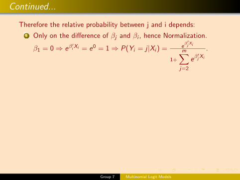
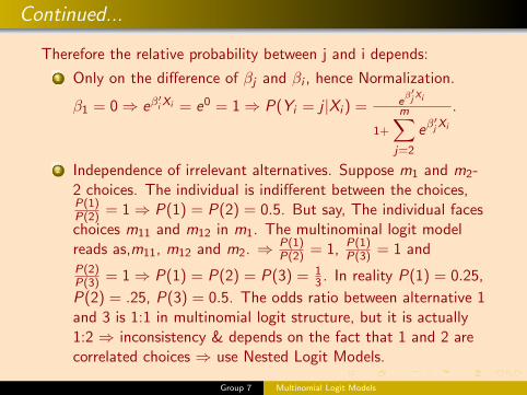
Therefore the relative probability between j and i depends:
1 Only on the difference of βj and βi , hence Normalization.
β1 = 0⇒ eβ′iXi = e0 = 1⇒ P(Yi = j |Xi ) = e
β′j Xi
1+
m∑j=2
eβ′jXi
.
2 Independence of irrelevant alternatives. Suppose m1 and m2-2 choices. The individual is indifferent between the choices,P(1)P(2) = 1⇒ P(1) = P(2) = 0.5. But say, The individual faceschoices m11 and m12 in m1. The multinominal logit modelreads as,m11, m12 and m2. ⇒ P(1)
P(2) = 1, P(1)P(3) = 1 and
P(2)P(3) = 1⇒ P(1) = P(2) = P(3) = 1
3 . In reality P(1) = 0.25,
P(2) = .25, P(3) = 0.5. The odds ratio between alternative 1and 3 is 1:1 in multinomial logit structure, but it is actually1:2 ⇒ inconsistency & depends on the fact that 1 and 2 arecorrelated choices ⇒ use Nested Logit Models.
Group 7 Multinomial Logit Models
Continued...
Therefore the relative probability between j and i depends:
1 Only on the difference of βj and βi , hence Normalization.
β1 = 0⇒ eβ′iXi = e0 = 1⇒ P(Yi = j |Xi ) = e
β′j Xi
1+
m∑j=2
eβ′jXi
.
2 Independence of irrelevant alternatives. Suppose m1 and m2-2 choices. The individual is indifferent between the choices,P(1)P(2) = 1⇒ P(1) = P(2) = 0.5. But say, The individual faceschoices m11 and m12 in m1. The multinominal logit modelreads as,m11, m12 and m2. ⇒ P(1)
P(2) = 1, P(1)P(3) = 1 and
P(2)P(3) = 1⇒ P(1) = P(2) = P(3) = 1
3 . In reality P(1) = 0.25,
P(2) = .25, P(3) = 0.5. The odds ratio between alternative 1and 3 is 1:1 in multinomial logit structure, but it is actually1:2 ⇒ inconsistency & depends on the fact that 1 and 2 arecorrelated choices ⇒ use Nested Logit Models.
Group 7 Multinomial Logit Models
ESTIMATION
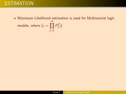
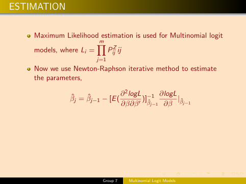
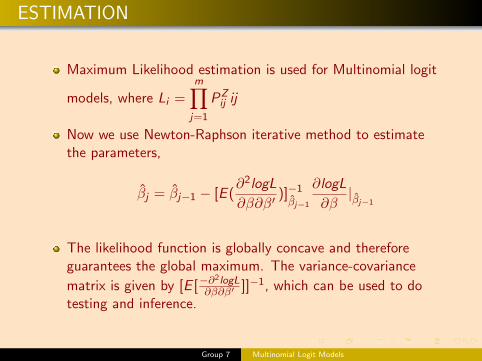
Maximum Likelihood estimation is used for Multinomial logit
models, where Li =m∏j=1
PZij ij
Now we use Newton-Raphson iterative method to estimatethe parameters,
β̂j = β̂j−1 − [E (∂2logL
∂β∂β′)]−1β̂j−1
∂logL
∂β|β̂j−1
The likelihood function is globally concave and thereforeguarantees the global maximum. The variance-covariance
matrix is given by [E [−∂2logL
∂β∂β′ ]]−1, which can be used to dotesting and inference.
Group 7 Multinomial Logit Models
ESTIMATION
Maximum Likelihood estimation is used for Multinomial logit
models, where Li =m∏j=1
PZij ij
Now we use Newton-Raphson iterative method to estimatethe parameters,
β̂j = β̂j−1 − [E (∂2logL
∂β∂β′)]−1β̂j−1
∂logL
∂β|β̂j−1
The likelihood function is globally concave and thereforeguarantees the global maximum. The variance-covariance
matrix is given by [E [−∂2logL
∂β∂β′ ]]−1, which can be used to dotesting and inference.
Group 7 Multinomial Logit Models

MODELLINGGL: CANDY CHOICE
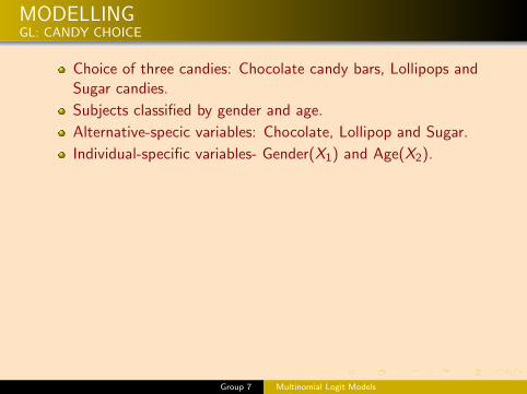
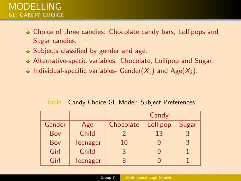
Choice of three candies: Chocolate candy bars, Lollipops andSugar candies.
Subjects classified by gender and age.
Alternative-specic variables: Chocolate, Lollipop and Sugar.
Individual-specific variables- Gender(X1) and Age(X2).
Table : Candy Choice GL Model: Subject Preferences
Candy
Gender Age Chocolate Lollipop SugarBoy Child 2 13 3Boy Teenager 10 9 3Girl Child 3 9 1Girl Teenager 8 0 1
Group 7 Multinomial Logit Models

MODELLINGGL: CANDY CHOICE
Choice of three candies: Chocolate candy bars, Lollipops andSugar candies.
Subjects classified by gender and age.
Alternative-specic variables: Chocolate, Lollipop and Sugar.
Individual-specific variables- Gender(X1) and Age(X2).
Table : Candy Choice GL Model: Subject Preferences
Candy
Gender Age Chocolate Lollipop SugarBoy Child 2 13 3Boy Teenager 10 9 3Girl Child 3 9 1Girl Teenager 8 0 1
Group 7 Multinomial Logit Models
Continued...GL: CANDY CHOICE ESTIMATION
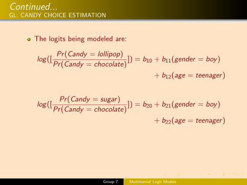
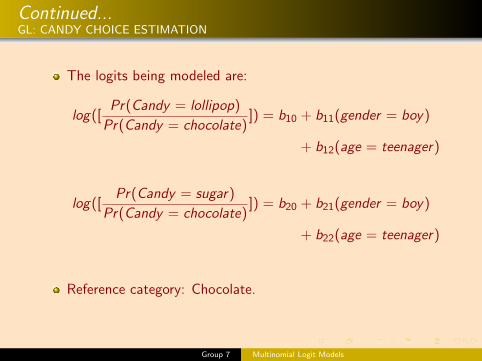
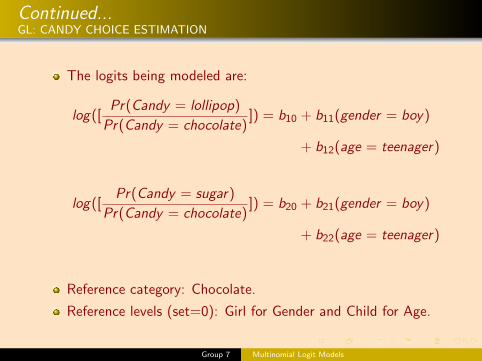
The logits being modeled are:
log([Pr(Candy = lollipop)
Pr(Candy = chocolate)]) = b10 + b11(gender = boy)
+ b12(age = teenager)
log([Pr(Candy = sugar)
Pr(Candy = chocolate)]) = b20 + b21(gender = boy)
+ b22(age = teenager)
Reference category: Chocolate.
Reference levels (set=0): Girl for Gender and Child for Age.
Group 7 Multinomial Logit Models
Continued...GL: CANDY CHOICE ESTIMATION
The logits being modeled are:
log([Pr(Candy = lollipop)
Pr(Candy = chocolate)]) = b10 + b11(gender = boy)
+ b12(age = teenager)
log([Pr(Candy = sugar)
Pr(Candy = chocolate)]) = b20 + b21(gender = boy)
+ b22(age = teenager)
Reference category: Chocolate.
Reference levels (set=0): Girl for Gender and Child for Age.
Group 7 Multinomial Logit Models
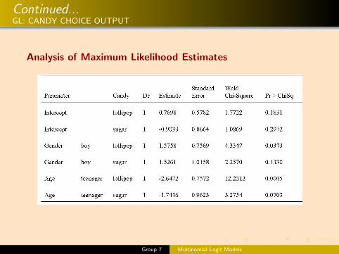
Continued...GL: CANDY CHOICE OUTPUT
Analysis of Maximum Likelihood Estimates
Group 7 Multinomial Logit Models
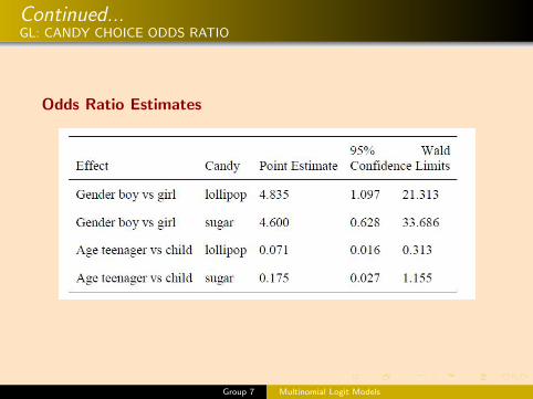
Continued...GL: CANDY CHOICE ODDS RATIO
Odds Ratio Estimates
Group 7 Multinomial Logit Models
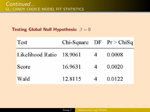
Continued...GL: CANDY CHOICE MODEL FIT STATISTICS
Testing Global Null Hypothesis: β = 0
Group 7 Multinomial Logit Models
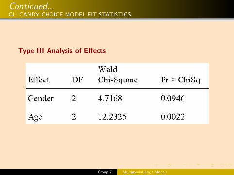
Continued...GL: CANDY CHOICE MODEL FIT STATISTICS
Type III Analysis of Effects
Group 7 Multinomial Logit Models
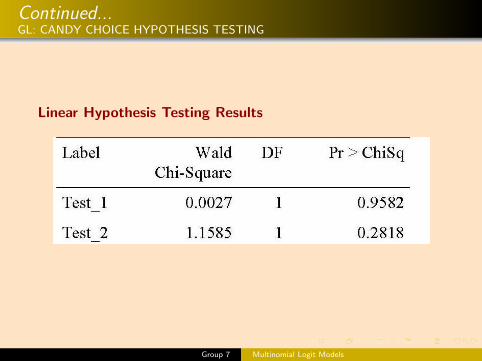
Continued...GL: CANDY CHOICE HYPOTHESIS TESTING
Linear Hypothesis Testing Results
Group 7 Multinomial Logit Models
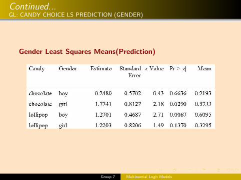
Continued...GL: CANDY CHOICE LS PREDICTION (GENDER)
Gender Least Squares Means(Prediction)
Group 7 Multinomial Logit Models
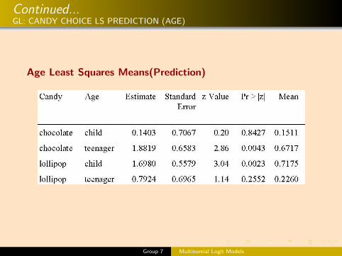
Continued...GL: CANDY CHOICE LS PREDICTION (AGE)
Age Least Squares Means(Prediction)
Group 7 Multinomial Logit Models

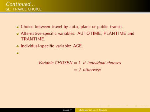
Continued...GL: TRAVEL CHOICE
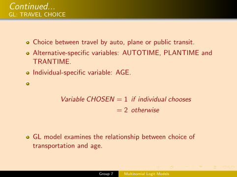
Choice between travel by auto, plane or public transit.
Alternative-specific variables: AUTOTIME, PLANTIME andTRANTIME.
Individual-specific variable: AGE.
Variable CHOSEN = 1 if individual chooses
= 2 otherwise
GL model examines the relationship between choice oftransportation and age.
Group 7 Multinomial Logit Models

Continued...GL: TRAVEL CHOICE
Choice between travel by auto, plane or public transit.
Alternative-specific variables: AUTOTIME, PLANTIME andTRANTIME.
Individual-specific variable: AGE.
Variable CHOSEN = 1 if individual chooses
= 2 otherwise
GL model examines the relationship between choice oftransportation and age.
Group 7 Multinomial Logit Models
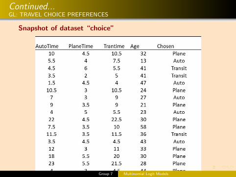
Continued...GL: TRAVEL CHOICE PREFERENCES
Snapshot of dataset “choice”
Group 7 Multinomial Logit Models
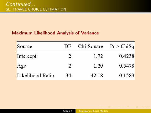
Continued...GL: TRAVEL CHOICE ESTIMATION
Maximum Likelihood Analysis of Variance
Group 7 Multinomial Logit Models
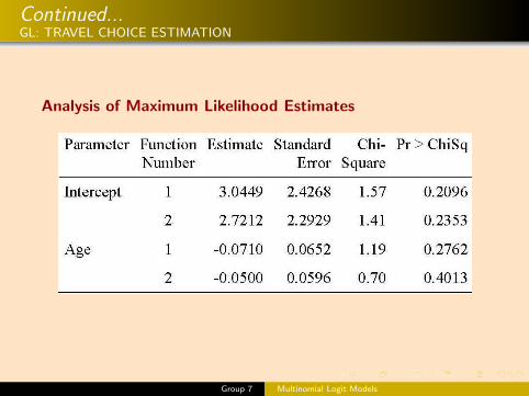
Continued...GL: TRAVEL CHOICE ESTIMATION
Analysis of Maximum Likelihood Estimates
Group 7 Multinomial Logit Models
Continued...GL: TRAVEL CHOICE PREDICTION
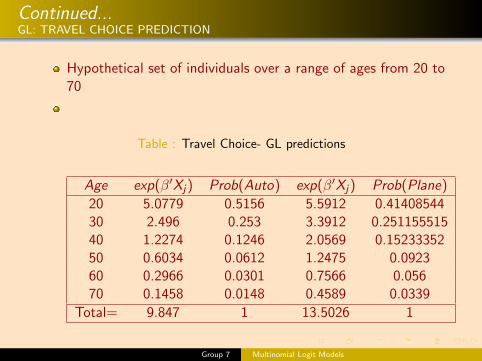
Hypothetical set of individuals over a range of ages from 20 to70
Table : Travel Choice- GL predictions
Age exp(β′Xj) Prob(Auto) exp(β′Xj) Prob(Plane)
20 5.0779 0.5156 5.5912 0.4140854430 2.496 0.253 3.3912 0.25115551540 1.2274 0.1246 2.0569 0.1523335250 0.6034 0.0612 1.2475 0.092360 0.2966 0.0301 0.7566 0.05670 0.1458 0.0148 0.4589 0.0339
Total= 9.847 1 13.5026 1
Group 7 Multinomial Logit Models
Continued...GL: TRAVEL CHOICE PREDICTION
Hypothetical set of individuals over a range of ages from 20 to70
Table : Travel Choice- GL predictions
Age exp(β′Xj) Prob(Auto) exp(β′Xj) Prob(Plane)
20 5.0779 0.5156 5.5912 0.4140854430 2.496 0.253 3.3912 0.25115551540 1.2274 0.1246 2.0569 0.1523335250 0.6034 0.0612 1.2475 0.092360 0.2966 0.0301 0.7566 0.05670 0.1458 0.0148 0.4589 0.0339
Total= 9.847 1 13.5026 1
Group 7 Multinomial Logit Models
Continued...CL: CANDY CHOICE
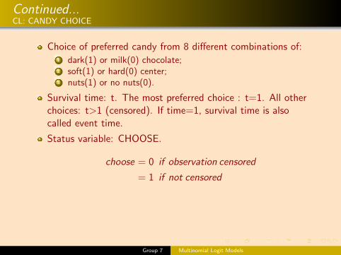
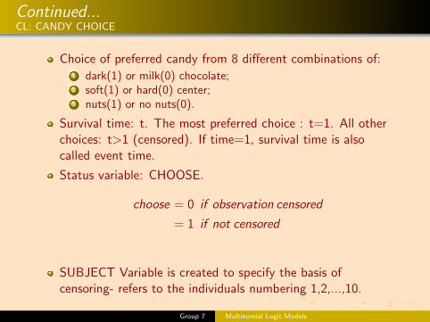
Choice of preferred candy from 8 different combinations of:1 dark(1) or milk(0) chocolate;2 soft(1) or hard(0) center;3 nuts(1) or no nuts(0).
Survival time: t. The most preferred choice : t=1. All otherchoices: t>1 (censored). If time=1, survival time is alsocalled event time.
Status variable: CHOOSE.
choose = 0 if observation censored
= 1 if not censored
SUBJECT Variable is created to specify the basis ofcensoring- refers to the individuals numbering 1,2,...,10.
Group 7 Multinomial Logit Models
Continued...CL: CANDY CHOICE
Choice of preferred candy from 8 different combinations of:1 dark(1) or milk(0) chocolate;2 soft(1) or hard(0) center;3 nuts(1) or no nuts(0).
Survival time: t. The most preferred choice : t=1. All otherchoices: t>1 (censored). If time=1, survival time is alsocalled event time.
Status variable: CHOOSE.
choose = 0 if observation censored
= 1 if not censored
SUBJECT Variable is created to specify the basis ofcensoring- refers to the individuals numbering 1,2,...,10.
Group 7 Multinomial Logit Models
Continued...CL: CANDY CHOICE ESTIMATION
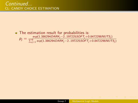
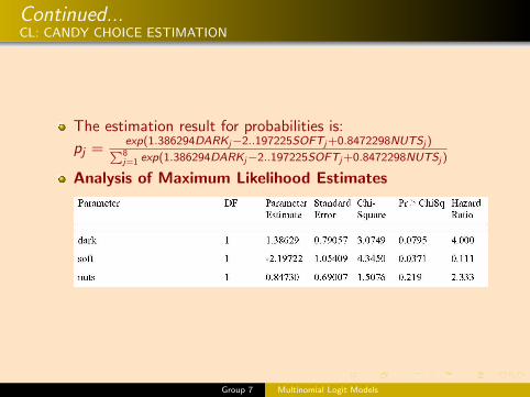
The estimation result for probabilities is:
pj =exp(1.386294DARKj−2..197225SOFTj+0.8472298NUTSj )∑8j=1 exp(1.386294DARKj−2..197225SOFTj+0.8472298NUTSj )
Analysis of Maximum Likelihood Estimates
Group 7 Multinomial Logit Models
Continued...CL: CANDY CHOICE ESTIMATION
The estimation result for probabilities is:
pj =exp(1.386294DARKj−2..197225SOFTj+0.8472298NUTSj )∑8j=1 exp(1.386294DARKj−2..197225SOFTj+0.8472298NUTSj )
Analysis of Maximum Likelihood Estimates
Group 7 Multinomial Logit Models
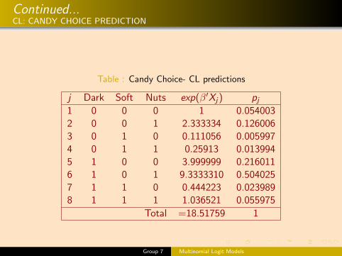
Continued...CL: CANDY CHOICE PREDICTION
Table : Candy Choice- CL predictions
j Dark Soft Nuts exp(β′Xj) pj1 0 0 0 1 0.0540032 0 0 1 2.333334 0.1260063 0 1 0 0.111056 0.0059974 0 1 1 0.25913 0.0139945 1 0 0 3.999999 0.2160116 1 0 1 9.3333310 0.5040257 1 1 0 0.444223 0.0239898 1 1 1 1.036521 0.055975
Total =18.51759 1
Group 7 Multinomial Logit Models
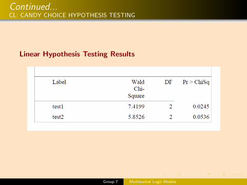
Continued...CL: CANDY CHOICE HYPOTHESIS TESTING
Linear Hypothesis Testing Results
Group 7 Multinomial Logit Models

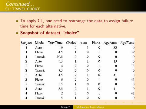
Continued...CL: TRAVEL CHOICE
To apply CL, one need to rearrange the data to assign failuretime for each alternative.
Snapshot of dataset “choice”
Group 7 Multinomial Logit Models
Continued...CL: TRAVEL CHOICE
To apply CL, one need to rearrange the data to assign failuretime for each alternative.
Snapshot of dataset “choice”
Group 7 Multinomial Logit Models
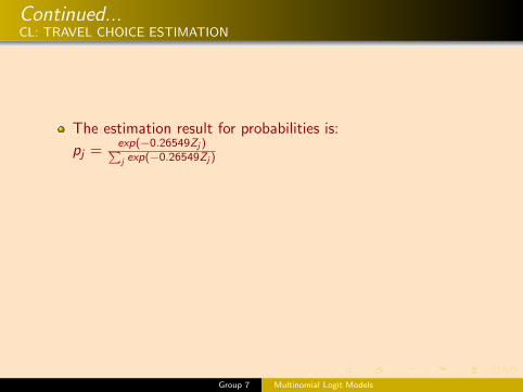
Continued...CL: TRAVEL CHOICE ESTIMATION
The estimation result for probabilities is:
pj =exp(−0.26549Zj )∑j exp(−0.26549Zj )
Analysis of Maximum Likelihood Estimates
Group 7 Multinomial Logit Models
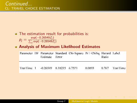
Continued...CL: TRAVEL CHOICE ESTIMATION
The estimation result for probabilities is:
pj =exp(−0.26549Zj )∑j exp(−0.26549Zj )
Analysis of Maximum Likelihood Estimates
Group 7 Multinomial Logit Models
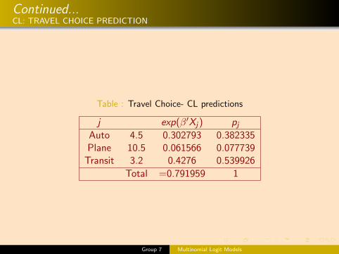
Continued...CL: TRAVEL CHOICE PREDICTION
Table : Travel Choice- CL predictions
j exp(β′Xj) pjAuto 4.5 0.302793 0.382335Plane 10.5 0.061566 0.077739
Transit 3.2 0.4276 0.539926
Total =0.791959 1
Group 7 Multinomial Logit Models
Continued...ML: TRAVEL CHOICE
Incorporates both types of variables: age and travel time.
New variables AgeAuto and AgePlane, each of whichrepresent the products of the individual’s age and his failuretime for each choice.
Group 7 Multinomial Logit Models

Continued...ML: TRAVEL CHOICE
Incorporates both types of variables: age and travel time.
New variables AgeAuto and AgePlane, each of whichrepresent the products of the individual’s age and his failuretime for each choice.
Group 7 Multinomial Logit Models
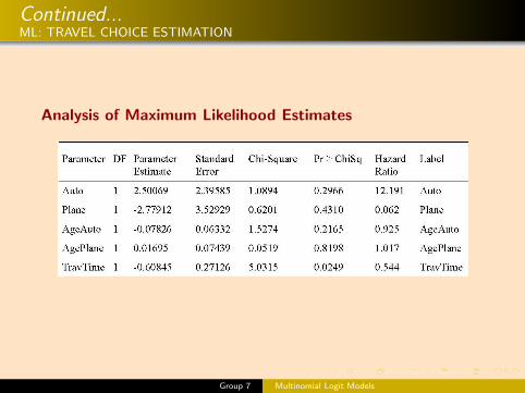
Continued...ML: TRAVEL CHOICE ESTIMATION
Analysis of Maximum Likelihood Estimates
Group 7 Multinomial Logit Models
CONCLUSION
We demonstrate the applications of the three types ofMultinomial Logit models through examples to show theprediction of choices or responses of individuals.
Such models has widespread applications in the study ofconsumer preferences, levels of academic achievements,gender based differences in outcomes, medical research andvarious areas of behavioural economics.
The assumptions underlying the Multinomial Logit Modeloften do not hold in practice- Independence of irrelevantalternatives (wayout Nested Logit) and Influences of pastchoices (wayout Multinomial probit).
Group 7 Multinomial Logit Models
REFERENCES & WEBSITES
SAS/STAT Software: Changes and Enhancements, Release8.2.
SAS, 1995, Logistic Regression Examples Using the SASSystem, pp. (2-3).
Lecture notes of Dr. Subrata Sarkar.
So Y. and Kuhfeld W. F., “Multinomial Logit Models”, 2010,presented at SUGI 20.
Starkweather, J. and Moske, A., “Multinomial LogitisticRegression”, 2011.
www.ats.ucla.edu
www.wikipedia.com
Group 7 Multinomial Logit Models

Thank you...
Group 7 Multinomial Logit Models