(+multinomial, ordered, conditional) - harry ganzeboom - logistic... · logistic regression:...

Logistic regression: binomial (+multinomial, ordered, conditional)

Harry Ganzeboom

March 12 2009RESMA Course Data Analysis & Report #6

Logistic regression 2

OLS assumptions

• Dependent variable is a score:– Continuous– Unbounded– Varies linear with the predictor variable.

• However, our variables in fact are often a choice among categories:– Discrete– Limited range– Often have a (partial) rank-order and sometimes have a distance– May associate with predictor variables in irregular (non-linear) ways.

• Important special case: outcome variable is 0/1 (binary, binomial). Not: dummy.


Variations in SPSS

• LOGISTIC: for binary outcome variables• NOMREG: for multinomial outcome variables.• PLUM: for ordered multinomial outcome

variables.• LOGLINEAR: all sort of models, but discrete

independent variables.• All these programs will do binary logistic

regression as a special case. The coefficients may look different (see O’Connell and excercise).


0/1 dichotomy as dependent variable in OLS

• If you use OLS to model 0/1 outcomes (the ‘linear probability’ model), the following problems will arise:– The OLS assumption of homoskedasticity will not apply: the

variation is very small at the extremes. This will bias the coefficients and invalidate the SE estimates.

– Predicted values may occur outside the 0/1 range.

• Both problems are most severe when you are modeling a variable that has an expected value (=mean) close to 0 or 1. This happens often in event analysis (next course).

• However, when you are modeling a variable in the 0.20..0.80 range, the ‘linear probability model’ is in fact quite useful, at least to look at.


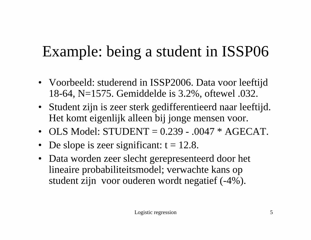
Example: being a student in ISSP06

• Voorbeeld: studerend in ISSP2006. Data voor leeftijd18-64, N=1575. Gemiddelde is 3.2%, oftewel .032.

• Student zijn is zeer sterk gedifferentieerd naar leeftijd.Het komt eigenlijk alleen bij jonge mensen voor.

• OLS Model: STUDENT = 0.239 - .0047 * AGECAT.• De slope is zeer significant: t = 12.8.• Data worden zeer slecht gerepresenteerd door het

lineaire probabiliteitsmodel; verwachte kans op student zijn voor ouderen wordt negatief (-4%).


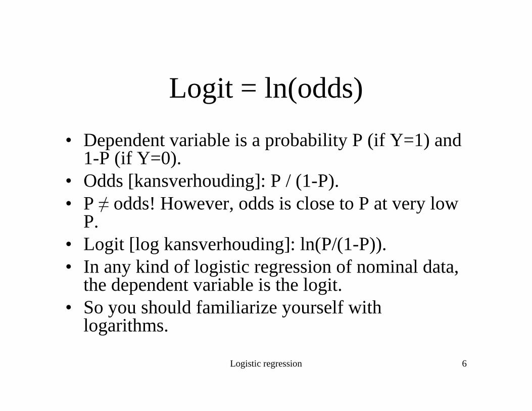
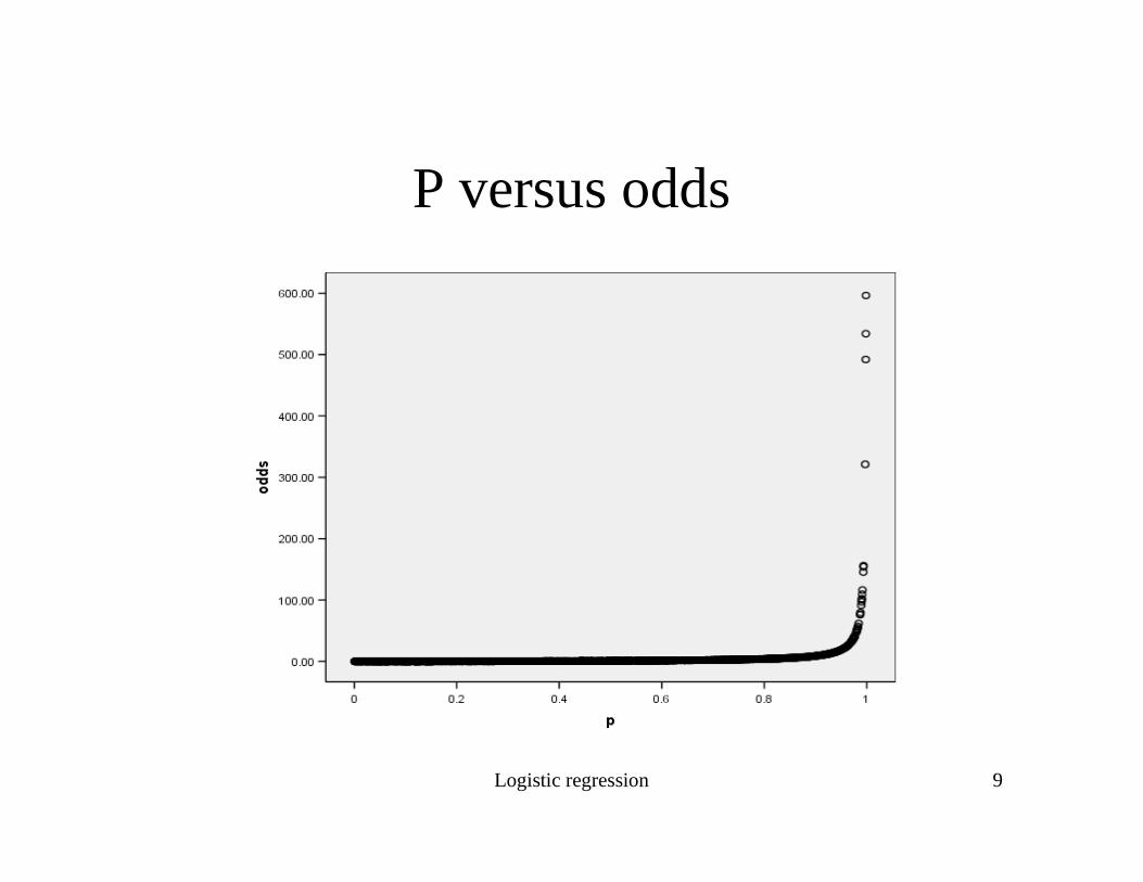
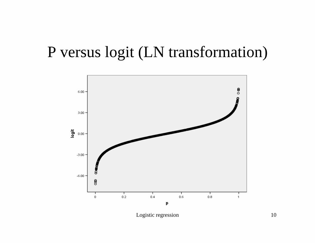
Logit = ln(odds)

• Dependent variable is a probability P (if Y=1) and 1-P (if Y=0).

• Odds [kansverhouding]: P / (1-P). • P ≠ odds! However, odds is close to P at very low

P.• Logit [log kansverhouding]: ln(P/(1-P)).• In any kind of logistic regression of nominal data,

the dependent variable is the logit.• So you should familiarize yourself with

logarithms.


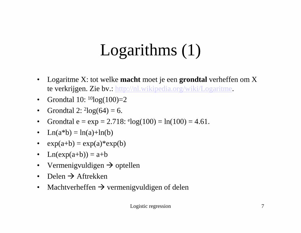
Logarithms (1)

• Logaritme X: tot welkemacht moet je eengrondtal verheffen om X te verkrijgen. Zie bv.: http://nl.wikipedia.org/wiki/Logaritme.

• Grondtal 10: 10log(100)=2

• Grondtal 2: 2log(64) = 6.

• Grondtal e = exp = 2.718:elog(100) = ln(100) = 4.61.

• Ln(a*b) = ln(a)+ln(b)

• exp(a+b) = exp(a)*exp(b)

• Ln(exp(a+b)) = a+b

• Vermenigvuldigen� optellen

• Delen� Aftrekken

• Machtverheffen� vermenigvuldigen of delen


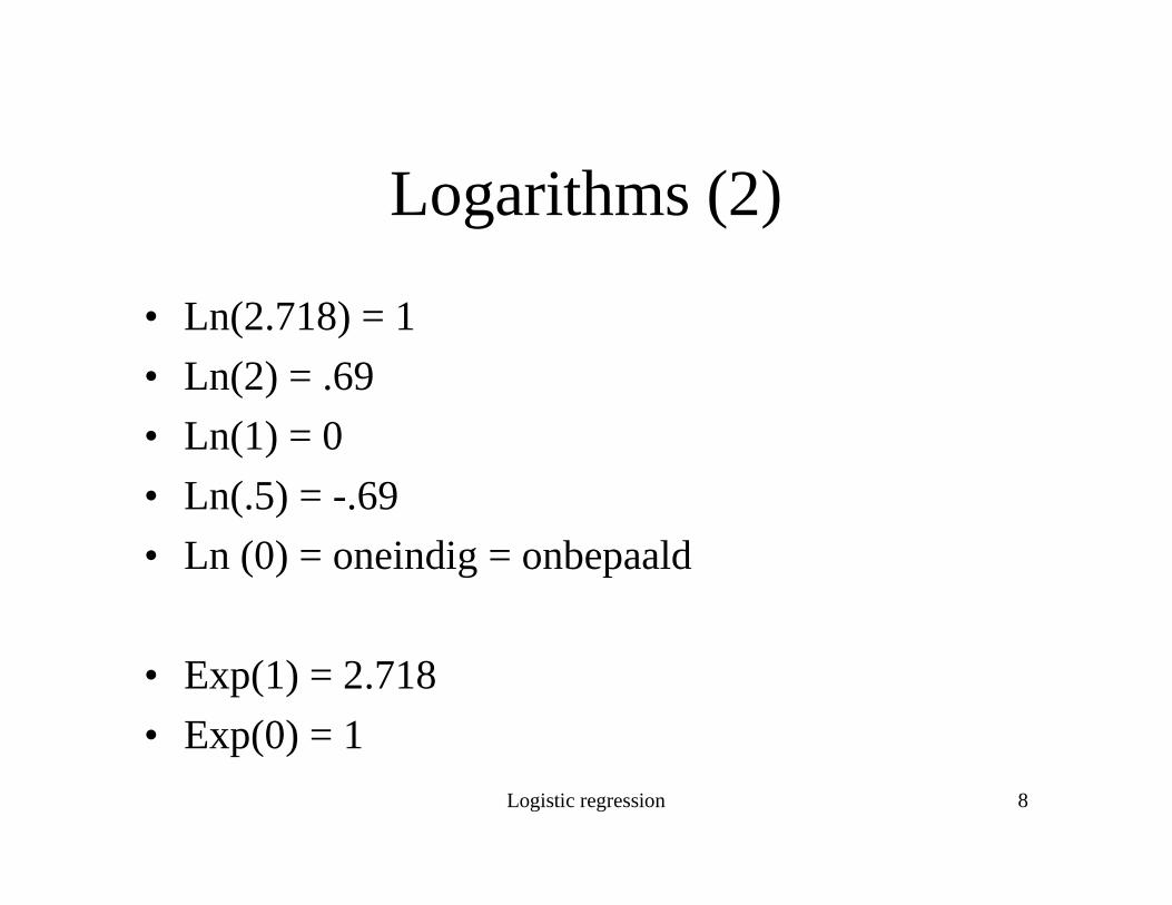
Logarithms (2)

• Ln(2.718) = 1

• Ln(2) = .69

• Ln(1) = 0

• Ln(.5) = -.69

• Ln (0) = oneindig = onbepaald

• Exp(1) = 2.718

• Exp(0) = 1


P versus odds


P versus logit (LN transformation)


Logit versus P


Logit, odds, and P

• Logit = ln(odd) = ln (P/(1-P)).

• Exp(logit) � odds.

• Ln(odds) � logit.

• P = 1 / (1+exp(-logit))

• (this transformation will SPSS do for you in ‘predicted value’).


Logistic regression in SPSS

• Analyze > regression > binary logistic

• The syntax of the model is different from REGR, but similar to UNIANOVA:– Logistic Y with X1 X2. [additive, linear]– Logistic Y with X1 X2 C1 /cat=C1. [+

categorical]– Logistic Y with X1 X2 C1 X2*C1 /cat=C1. [+interaction]

• So, syntax provides for (A) automatic creation of dummy variables, and (B) automatic creation of interaction terms.


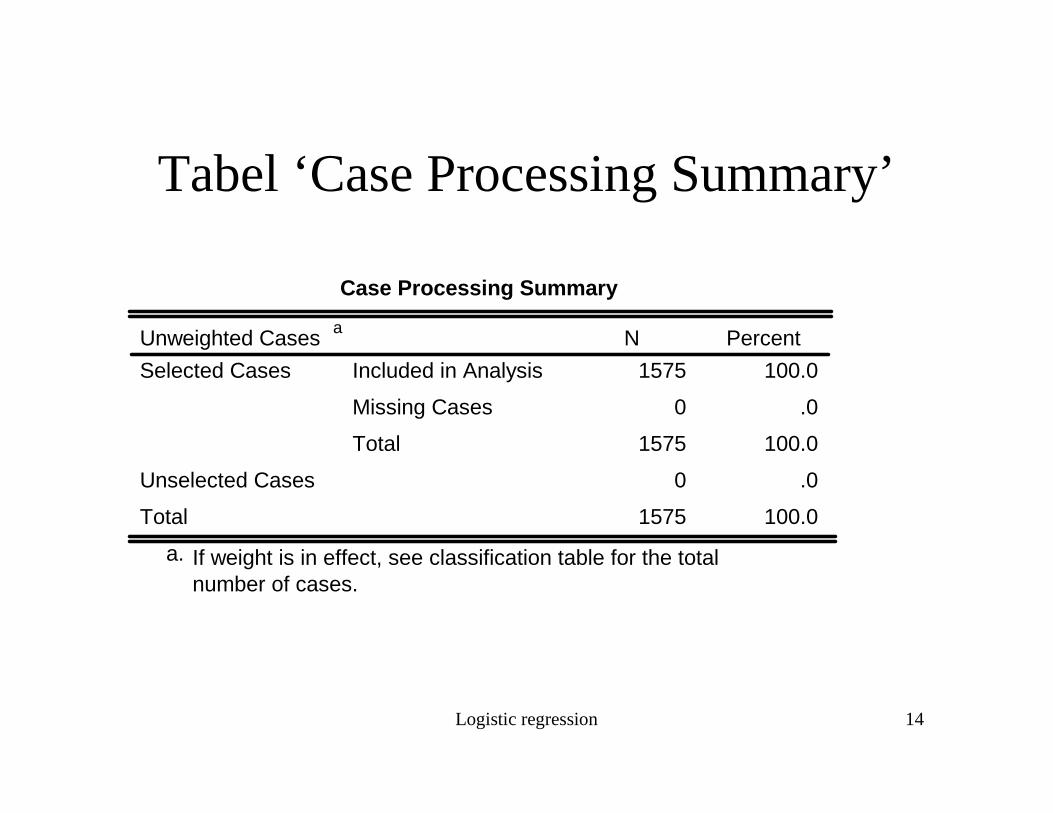
Tabel ‘Case Processing Summary’

Case Processing Summary

1575 100.0

0 .0

1575 100.0

0 .0

1575 100.0

Unweighted Cases a

Included in Analysis

Missing Cases

Total

Selected Cases

Unselected Cases

Total

N Percent

If weight is in effect, see classification table for the totalnumber of cases.

a.


Tabel ‘Dependent Variable Encoding’

Dependent Variable Encoding

0

1

Original Value

0

1

Internal Value


Tabel ‘Omnibus Tests of Model coefficients’

Omnibus Tests of Model Coefficients

187.933 1 .000

187.933 1 .000

187.933 1 .000

Step

Block

Model

Step 1

Chi-square df Sig.


Tabel ‘Model Summary’

Model Summary

255.462a .112 .458

Step

1

-2 Loglikelihood

Cox & SnellR Square

Nagelkerke RSquare

Estimation terminated at iteration number 9 becauseparameter estimates changed by less than .001.

a.


Tabel ‘Classification Table’

Classification Tablea

1518 7 99.5

35 15 30.0

97.3

Observed

0

1

unempl

Overall Percentage

Step 1

0 1

unempl PercentageCorrect

Predicted

The cut value is .500a.


Some good advice

• Do not leave the coding of the dependent variable to the program.

• Missing values always need scrutiny. There is no pairwiseoption. Use substitution to see effects of missing values patterns.

• Like in OLS, life becomes happier when you code your independent variables using a 0 and an interpretable unit.

• Significance of individual coefficients: t = b/SE.

• With some practice, the multiplicative coefficients are easier to talk about than the logistic ones.


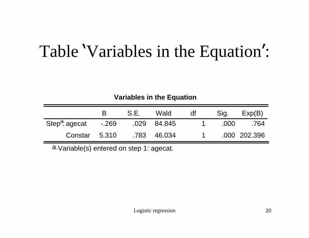
Table ‘Variables in the Equation’:

Variables in the Equation

-.269 .029 84.845 1 .000 .764

5.310 .783 46.034 1 .000 202.396

agecat

Constant

Step 1aB S.E. Wald df Sig. Exp(B)

Variable(s) entered on step 1: agecat.a.


Logistische en multiplicatieve regressiecoëfficiënten

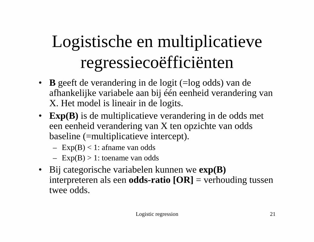
• B geeft de verandering in de logit (=log odds) van de afhankelijke variabele aan bij één eenheid verandering van X. Het model is lineair in de logits.

• Exp(B) is de multiplicatieve verandering in de odds met een eenheid verandering van X ten opzichte van odds baseline (=multiplicatieve intercept).– Exp(B) < 1: afname van odds– Exp(B) > 1: toename van odds

• Bij categorische variabelen kunnen we exp(B)interpreteren als eenodds-ratio [OR] = verhouding tussentwee odds.


Multiplicatievecoefficientenen de odds-ratio OR

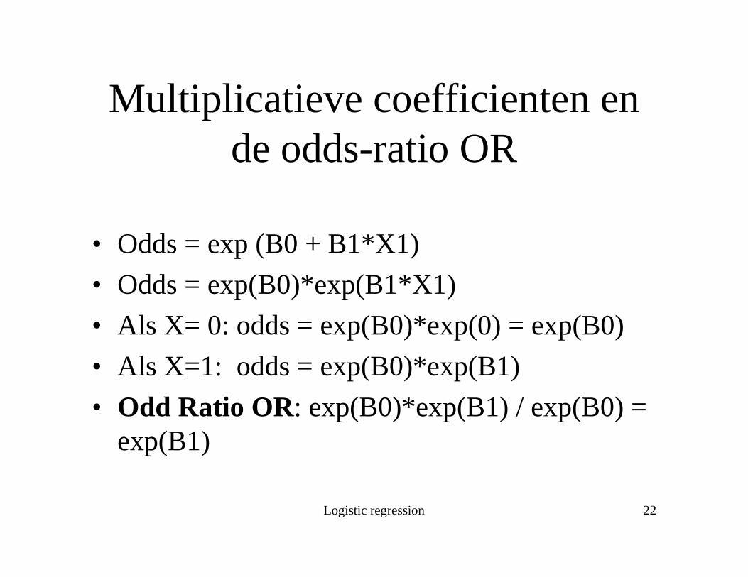
• Odds = exp (B0 + B1*X1)

• Odds = exp(B0)*exp(B1*X1)

• Als X= 0: odds = exp(B0)*exp(0) = exp(B0)

• Als X=1: odds = exp(B0)*exp(B1)

• Odd Ratio OR: exp(B0)*exp(B1) / exp(B0) = exp(B1)


GeengestandaardiseerdeB’s

• Anders dan bij OLS heeft logistic geengestandaardiseerde coefficienten.

• B’s zijn daaromalleen met elkaar vergelijkbaar alshun eenheden vergelijkbaar zijn.

• Wil je toch gestandaardiseerde coefficientenhebben, dan zul je eerst zelf de X-en moetenstandaardiseren (=voorzien van vergelijkbaremeeteenheid).


Inferentielestatistiek

• Logistic geeft niet de bij OLS gebruikelijke T-toets: t = B/SE. Deze kun je wel zelf berekenen.

• Wald statistic is t2. Vergelijk met Chi2 of F-tabelmet 1, veel vrijheidsgraden. Kritieke waarde: 3.84.

• SE’s behoren horen bij logits. Betrouwbaarheids-intervalllen rondomlogits zijn symmetrisch, rondommultiplicatieve coefficienten zijn zeasymmetrisch.


Logistischeregressiemet nominaleonafhankelijkevariabelen

• Bij logistic behoef je niet zelf dummy-variabelenaan te maken by categorische X (het mag wel).

• ../cat=X1 /contrast(X1)=indicator(1)geeft aan dat X1 categorisch is en 1 de referentie-categorie is.

• De output kan behoorlijk verwarrend zijn. Let goed op de “Categorical variable codings”.

• De Wald statistic is nu een test op gezamenlijkebijdrage van de dummy-variabelen.


Tabel ‘Categorical variable codings’

Categorical Variables Codings

22 .000 .000 .000 .000 .000

53 1.000 .000 .000 .000 .000

276 .000 1.000 .000 .000 .000

453 .000 .000 1.000 .000 .000

379 .000 .000 .000 1.000 .000

363 .000 .000 .000 .000 1.000

19

22

30

40

50

60

agecat

Frequency (1) (2) (3) (4) (5)

Parameter coding


Homework

• Read O’Connell 1-27.

• Practice the use of binary logistic in outcome ‘University education’ with AGE and FEMALE in ESS, using LOGIST, NOMREG and PLUM. I will send aroundfurther specification.

(+multinomial, ordered, conditional) - harry ganzeboom - logistic... · logistic regression:...

Documents