multiple imputation with diagnostics (mi) in r: opening ...gelman/research/published/mipaper.pdf ·...

JSS Journal of Statistical Software

December 2011, Volume 45, Issue 2. http://www.jstatsoft.org/

Multiple Imputation with Diagnostics (mi) in R:Opening Windows into the Black Box

Yu-Sung SuTsinghua University

Andrew GelmanColumbia University

Jennifer HillNew York University

Masanao YajimaUniversity of California, Los Angeles

Abstract

Our mi package in R has several features that allow the user to get inside the impu-tation process and evaluate the reasonableness of the resulting models and imputations.These features include: choice of predictors, models, and transformations for chained im-putation models; standard and binned residual plots for checking the fit of the conditionaldistributions used for imputation; and plots for comparing the distributions of observedand imputed data. In addition, we use Bayesian models and weakly informative priordistributions to construct more stable estimates of imputation models. Our goal is tohave a demonstration package that (a) avoids many of the practical problems that arisewith existing multivariate imputation programs, and (b) demonstrates state-of-the-art di-agnostics that can be applied more generally and can be incorporated into the softwareof others.

Keywords: multiple imputation, model diagnostics, chained equations, weakly informativeprior, mi, R.

1. Introduction

The general statistical theory and framework for managing missing information has been welldeveloped since Rubin (1987) published his pioneering treatment of multiple imputation meth-ods for nonresponse in surveys. Several software packages have been developed to implementthese methods to deal with incomplete datasets. However, each of these imputation packagesis, to a certain degree, a black box, and the user must trust the imputation procedure withoutmuch control over what goes into it and without much understanding of what comes out.

http://www.jstatsoft.org/

2 mi: Multiple Imputation with Diagnostics in R

Model checking and other diagnostics are generally an important part of any statistical pro-cedure. Examining the implications of imputations is particularly important because of theinherent tension of multiple imputation: that the model used for the imputations is not ingeneral the same as the model used for the analysis (Meng 1994; Fay 1996; Robins and Wang2000). We have created an open-ended, open source mi package, not only to solve theseimputation problems, but also to develop and implement new ideas in modeling and modelchecking.

Our mi package in R (R Development Core Team 2011) has several features that allow the userto get inside the imputation process and evaluate the reasonableness of the resulting modeland imputations. These features include: choice of predictors, models, and transformationsfor chained imputation models; standard and binned residual plots for checking the fit of theconditional distributions used for imputation; and plots for comparing the distributions ofobserved and imputed data. mi uses an algorithm known as a chained equation approach(Buuren and Groothuis-Oudshoorn 2011; Raghunathan, Lepkowski, Van Hoewyk, and Solen-berger 2001); the user specifies the conditional distribution of each variable with missingvalues conditioned on other variables in the data, and the imputation algorithm sequentiallyiterates through the variables to impute the missing values using the specified models.

We omit a description of the theoretical background of multiple imputation since this materialis available from many other sources (e.g., Little and Rubin (2002); Gelman and Hill (2007,chapter 25)). Rather, the major goal is to demonstrate the flexible way in which userscan perform multiple imputation with mi and to introduce functions for diagnostics afterimputation. The paper proceeds as follows: In Section 2, we provide an overview of steps toperform sensible multiple imputation. In Section 3, we demonstrate some novel features andfunctions of mi that address some imputation problems that have been neglected by othersoftware. These features include: (1) Bayesian regression models to address problems withseparation; (2) imputation steps that deal with semi-continuous data; (3) modeling strategiesthat handle issues of perfect correlation and structural correlation; (4) functions that check theconvergence of the imputations; and (5) plotting functions that visually check the imputationmodels. In Section 4, we demonstrate how to apply these functions using an example of a studyof people living with HIV in New York City (Messeri, Lee, Abramson, Aidala, Chiasson, andJessop 2003). In Section 5, we discuss future plans for ourmi package. The package is availablefrom the Comprehensive R Archive Network at http://CRAN.R-project.org/package=mi.

2. Basic setup

The procedure to obtain sensible multiply imputed datasets approach requires four steps:setup, imputation, analysis, and validation. Each step is divided into substeps as follows:

1. Setup.

Display of missing data patterns.

Identifying structural problems in the data and preprocessing.

Specifying the conditional models.

2. Imputation.

Iterative imputation based on the conditional model.

http://CRAN.R-project.org/package=mi

Journal of Statistical Software 3

Checking the fit of conditional models and checking to see if the imputed valuesare reasonable.

Checking the convergence of the procedure.

3. Analysis.

Obtaining completed data.

Pooling the complete case analysis on multiply imputed datasets.

4. Validation.

Sensitivity analysis.

Cross validation.

Compatibility check.

At first glance, it may seem more complicated to conduct multiple imputation using mi

compared to other available imputation software. However this is because we outline stepsthat other packages have traditionally ignored. mi is designed for both novice and experiencedusers. For the novice users, mi has a step-by-step interactive interface where users chooseoptions from the given multiple choices and a graphical user interface (GUI) where users clickbuttons (see Section 4). For more experienced users, mi has simple commands that users canuse to conduct a multiple imputation. This section simply describes the core functions. InSection 4, we will demonstrate how users can easily implement these imputation steps usingmi via an example.

The implementation of the mi package is straightforward. The core function is a genericfunction mi(object, ...) which executes one of three methods depending on whether theinput is a data.frame, or of S4 class mi.preprocessed, or mi. The mi.preprocessed classdefines the output return by mi.preprocess() when it recodes special variables in a dataset(see Section 2 and Section 3). The mi class defines the output returned by mi() when itfinishes a multiple imputation with a dataset. The usages of the S4 methods for signaturedata.frame, mi.preprocessed, and mi are described respectively below:

mi(object, info, n.imp = 3, n.iter = 30,

R.hat = 1.1, max.minutes = 20, rand.imp.method = "bootstrap",

preprocess = TRUE, run.past.convergence = FALSE,

seed = NA, check.coef.convergence = FALSE,

add.noise = noise.control())

mi(object, n.imp = 3, n.iter = 30,

R.hat = 1.1, max.minutes = 20, rand.imp.method = "bootstrap",

run.past.convergence = FALSE,

seed = NA, check.coef.convergence = FALSE,

add.noise = noise.control())

mi(object, info, n.iter = 30, R.hat = 1.1,

max.minutes = 20, rand.imp.method = "bootstrap",

run.past.convergence = FALSE, seed = NA)


object: A data frame or an mi object that contains an incomplete dataset. mi onlyrecognizes the special value NA as the missing data.

info: The mi.info matrix returned by mi.info(). This matrix contains informationabout the data (e.g., number of cells that are missing in a variable, variable types, etc.),and some parameters that control the imputation procedure (see Section 2).

n.imp: The number of independent imputation chains with di↵erent sets of startingvalues randomly drawn from the observed ones (see rand.imp.method). The defaultis 3 chains. A minimum of 2 chains are required in order to conduct the Gelman andRubin convergence diagnostic (Gelman and Rubin 1992; Gelman, Carlin, Stern, andRubin 2004).

n.iter: The maximum number of imputation iterations. The default is 30 iterations.

R.hat: The value of the R̂ statistic used as a convergence criterion. The default is 1.1(Gelman and Rubin 1992; Gelman, Carlin, Stern, and Rubin 2004).

max.minutes: The maximum number of minutes to operate the whole imputation pro-cess. The default is 20 minutes.

rand.imp.method: The method used for random imputing starting values of the missingvalues. Currently, mi() only implements the bootstrap method: missing values arefilled in with values that are randomly sampled from the observed data.

preprocess: Default is TRUE. mi() will transform the variables that are not of standarddistribution. These types of variable are nonnegative, positive-continuous, andproportion. The transformed variables then can be modeled using linear regression(see Section 3 for details).

run.past.convergence: Default is FALSE, meaning mi() stops if the imputation isconverged. If the value is TRUE, mi() will run until the values of either n.iter ormax.minutes are reached even if the imputation is converged.

seed: The random number seed. The default is NA.

check.coef.convergence: Default is FALSE. mi() only checks the convergence of themeans and standard deviations of the imputed values. If the value is TRUE, mi() alsochecks the convergence of the coe�cients of imputation models.

add.noise: A list of parameters for controlling the process of adding noise to mi() vianoise.control(). This is to fill in the missing values with values that are randomlysampled from the observed ones. This step addresses the problem of collinearity thatimpedes appropriate imputation of missing data (see Section 3 for details).

mi() is a wrapper of several key components: the imputation information matrix, variabletypes and imputation models.

2.1. Imputation information matrix

mi.info() produces a matrix of imputation information that is needed to impute the missingdata. After the information is extracted from a dataset, users can still alter the default model


specifications that are automatically created using this imputation information. Such a matrixof imputation information allows the users to have control over the imputation process. Itcontains the following information:

name: The names of variables in the dataset.

imp.order: A vector that records the order of each variable in the iterative imputationprocess. If such a variable is missing for all the observations (see all.missing), is anidentification variable (see is.ID), and is not included (see include), the imp.order

slot will record an NA.

nmis: A vector that records the number of data points that are missing in each variable.

type: A vector that contains the information of the variable types which are determinedby typecast() (see Section 2).

var.class: A vector that records the classes of the input variables.

level: A list of the levels of the input variables.

include: A vector of indicators that decide whether or not (Yes/No) to include a specificvariable in an imputation process. If include is No, the variable will not show up eitheras a predictor or as a variable to be imputed.

is.ID: A vector of indicators that determine whether or not (Yes/No) a specific variableis an identification (ID) variable. If a variable is detected as an ID variable, it will notbe included in the imputation process; thus the include slot records a No value. IDvariables are usually not problematic as dependent variables, since in most of the cases,they have no missing values. But when they are included in a model as predictors, theyinduce an unwanted order e↵ect of the data into the model (unless the data is a repeatedmeasure study and ID variables are treated as categorical variables). However, becauseID variables are hard to detect, users should carefully check to see if all such variableshave been detected.

all.missing: A vector of indictors that identify whether or not (Yes/No) a variable ismissing for all the observation. If the value is TRUE, such a variable will be excludedin the imputation process because it is not possible to impute sensible values. Theinclude slot records a No value if all.missing is TRUE.

missing.index: A vector that stores the index number of the missing units in a variable.

collinear: A vector of indicators that shows whether or not (Yes/No) a variable isperfectly collinear with another variable. mi.info() uses cor() to compute the Pearsoncoe�cients, a measure of the correlation (linear dependence) between two variables, ofthe data. If the Pearson coe�cients are larger than 0.99999 (arbitrary chosen as thedefault in mi), mi.info() sets the value of the collinear slot to TRUE. Such a variablewill be excluded in the imputation process (thus the include slot records a No value) ifand only if these two variables have the same missing data pattern, meaning that theyare missing in the same units.


imp.formula: A vector of formulas that records the imputation formulas used in theimputation models. This formula represents the linear specification of the appropriatemodel. For instance, for a binary variable this formula represents the linear function ofcovariates that is set equal to the logit of the expectation of the response variable.

determ.pred: The name of the corresponding correlated variable. This slot is NULL ifthere is no corresponding correlated variable as identified by cor().

params: A list of parameters to pass on to the imputation models.

other: Other options. This is currently not used.

Users can alter the mi.info matrix using update(). For instance, if we have a variable x1

in a dataset, and we do not want to include it in the imputation process, we can update theinclude slot of the mi.info matrix by:

R> info

names include order number.mis all.mis type collinear

1 x1 Yes 1 40 No continuous No


...

R> info <- update(info, "include", list("x1" = FALSE))

R> info


1 x1 No NA 40 No continuous No


...

2.2. Variable types

mi handles eleven variable types. Within mi(), mi.info() uses typecast() to automaticallyidentify eight di↵erent variable types; mi.preprocess() specifies the log-continuous typevia transformation (see Section 3). The variable types that are not automatically identifiedby typecast() are count and predictive-mean-matching type.1 These two types must beuser-specified via update(). typecast() identifies variable types using the rules depicted inFigure 1.

The rules, which typecast() uses to identify each variable type, are listed as follows:

1. fixed: Any variable that contains a single unique value.

2. binary: Any variable that contains two unique values.

1predictive-mean-matching is not really a variable type. We include it here to invoke mi() to fit a model

using the predictive mean matching method (see Section 2)


3. ordered-categorical: Any variable that has the ordered attribute that is determinedby is.ordered() in R. Or any numerical variable that has 3 to 5 unique values.

4. unordered-categorical: Any factor or character variable that is determined byis.character() or is.factor() in R. This type of variable often is not saved as acharacter or factor variable. Additionally, typecast() will identify a numeric unorderedcategorical variable as a continuous or an ordered categorical variable if users are notvigilant about identifying it. An unordered categorical variable, once is identified bytypecast() or is specified by user, it is going to be imputed with a multinomial log-linear model (see Section 2) but is included in the imputation models of other variablesas a factorized predictor (i.e., R will split this variable into the respective indicatorvariables).

5. proportion: Any numerical variable that has its values fall between 0 and 1, notincluding 0 and 1.

6. positive-continuous: Any numerical variable that is always positive and has morethan 5 unique values.

7. nonnegative: Any numerical variable that is always nonnegative and has more than5 unique values.

8. continuous: Any numerical variable that is modeled as continuous without transfor-mation.

9. log-continuous: log-scaled continuous variable, specified by mi.preprocess() (seeSection 3).

10. count: A user-specified variable type.

11. predictive-mean-matching: An user-specified variable type (see Section 2).

Once the variable type is determined by typecast(), the type information will be stored inthe mi.info matrix. Nonetheless, users can alter this default judgment. For instance, if riotis the number of riots in a specific year, its values are very likely to fall between 0 and anypositive integer. Hence, typecast() is going to identify riot as either ordered-categorical,positive-continuous or nonnegative type, depending on number of unique values it hasand whether or not its values contains 0. You can alter this judgment by updating the type

slot in a mi.info matrix as:

R> info

names include order number.mis all.mis type correlated

1 riot Yes 1 23 No nonnegative No

...

R> info <- update(info, "type", list("riot" = "count"))

R> info


L==1

L==2

is.character(x)

is.factor(x)

is.ordered(x)

is.numeric(x)

fixed

binary

unordered−categorical

unordered−categorical

ordered−categorical

continuous

proportion

ordered−categorical

positive−continuous

nonnegative

all(0<x<1)

2<L<=5

L>5 & all(x>0)

L>5 & all(x>=0) mi.preprocess()

binary

log−continuouslog−continuous

L=length(unique(x))x

Figure 1: Illustration of the rules of typecast() to identify and classify di↵erent variabletypes. mi currently handles eleven variable types: fixed, binary, unordered-categorical,ordered-categorical, proportion, positive-continuous, nonnegative, continuous,log-continuous, count, and predictive-mean-matching. But mi can only automaticallyidentify the first eight variable types. mi.preprocess() specifies log-continuous variabletype via transformation. Users have to specify count and predictive-mean-matching vari-able types manually via update() or interactively via mi.iteractive().


1 riot Yes 1 23 No count No

...

2.3. Imputation models

By default, mi chooses the conditional models via type.model(), a function that determineswhich imputation models to use based on the variable types determined by typecast(). Ta-ble 1 lists the default regression models corresponding to variable types. mi.fixed() justcopies the values from the observed one. mi.categorical() uses multinom() (multino-mial log-linear model, Venables and Ripley 2002) to impute unordered categorical variables.mi uses mi.continuous() to impute positive-continuous, nonnegative, and proportion

variable types.

mi.continuous(), mi.binary(), mi.count(), and mi.polr() fit Bayesian version of thegeneralized linear models (bayesglm() and bayespolr(), see Gelman, Jakulin, Pittau, andSu 2008) of arm (Gelman, Su, Yajima, Hill, Pittau, Kerman, and Zheng 2011). The Bayesianversion of the generalized linear model that we use is di↵erent from the classical generalizedlinear model in that it adds a Student-t prior on the regression coe�cients. Gelman, Jakulin,Pittau, and Su (2008) propose a new prior distribution for classical (nonhierarchical) logisticregression models, constructed by first scaling all nonbinary variables to have mean 0 andstandard deviation 0.5, and then placing an independent Student-t prior distribution on the


Variable types mi regression functionsbinary mi.binary

continuous mi.continuous

count mi.count

fixed mi.fixed

log-continuous mi.continuous

nonnegative mi.continuous

ordered-categorical mi.polr

unordered-categorical mi.categorical

positive-continuous mi.continuous

proportion mi.continuous

predictive-mean-matching mi.pmm

Table 1: List of mi regression functions, corresponding to variable types.

coe�cients. As a default choice, they recommend the Cauchy distribution with center 0 andscale 2.5. At the present time, mi() does not allow users to alter the priors.

While this is a reasonably wide selection of models, it is still possible that none providecompletely adequate fit for the data which could lead to improper imputation. Achievingappropriate fit can be particularly challenging when constraints exist in the data, when het-eroskedasticity exists in a model, when multiple modes exist or a variety of other modelingchallenges. To address this issue, mi o↵ers an option to impute these data using the predictivemean matching method (Rubin 1987; Heitjan and Little 1991; Schenker and Taylor 1996).The predictive mean matching method (mi.pmm()) works in the following way. For each ob-servation with a missing value on a given variable, we find the observation (from among thosewith observed values on that variable) with the closest predictive mean for that variable.The observed value from this “match” is then used as the imputed value. Currently, thesepredictions are obtained from bayesglm(). However, we plan to extend the predictive meanmatching options in the future. This method can be problematic when rates of missingnessare high or when the missing values fall outside the range of the observed data. We arecontinuing to develop more flexible imputation models to better address the issue of creatingappropriate imputations.

3. Novel features

Our mi has some novel features that address some open issues in multiple imputation.

3.1. Bayesian models to address problems with separation

Logistic regression, and more generally, discrete data models, commonly su↵er from the prob-lem of separation. This problem occurs whenever the outcome variable is perfectly predictedby a predictor or a linear combination of the predictors. This can happen even with a modestnumber of predictors, particularly if the proportion of “successes” in the response variable isrelatively close to 0 or 1. The risk of separation typically increases as the number of pre-dictors increases. However, multiple imputation is generally strengthened by including manyvariables, which can help to impute more precisely and also may help to satisfy the miss-


mi functions Bayesian functionsmi.continuous() bayesglm() with gaussian familymi.binary() bayesglm() with binomial family (default uses logit link)mi.count() bayesglm() with quasi-poisson family (overdispersed poisson)mi.polr() bayespolr()

Table 2: Lists of Bayesian generalized linear models used in mi regression functions.

ing at random assumption. When imputing large-scale surveys to create public-use multiplyimputed datasets, several hundred variables might need to be imputed. And it is unclearhow or if we should start discarding subsets of variables from some or all of the conditionalmodels. Separation problems can cause the chained equation algorithms to either fail orimpute unreasonable values. Moreover, even without perfect separation, imposing priors onregression coe�cients improves imputation in cases of near-separation and/or collinearity ornear-collinearity of predictors (Gelman, Jakulin, Pittau, and Su 2008).

To address problems with separation, we have augmented our mi to allow for Bayesian versionof the generalized linear models with Student-t prior distributions on regression coe�cients(the default prior uses t distribution with center 0, degree of freedom 1 and scale 2.5). Themodels, as implemented in the functions bayesglm() and bayespolr(), automatically handleseparation (Gelman, Jakulin, Pittau, and Su 2008). The corresponding imputation modelsare listed in Table 2.2

3.2. Imputing semi-continuous data with transformation

Semi-continuous data (positive-continuous, nonnegative and proportion variable typesin mi) are typically not modeled in a reasonable way in other imputation software. Thedi�culty comes from the fact that these kinds of data have bounds or truncations and arenot of standard distributions. Our algorithm models these data using transformations viami.preprocess(). These transformations are automatically performed in mi() by settingthe option preprocess = TRUE (which is the default).

For the nonnegative variable type, mi.preprocess() creates two ancillary variables. Oneis an indicator for which values of the nonnegative variable are greater than 0. The otherancillary variable takes the log of the original variable for any value that is greater than 0. Forthe positive-continuous variable type, mi.preprocess() takes the log of the variable. Forthe proportion variable type, mi.preprocess() does a logit transformation on the variable

as logit (x) = log⇣

x

1�x

⌘.

Figure 2 illustrates this transformation process. Users can transform the data back to the orig-inal scale using mi.postprocess(). This is implemented automatically in mi.completed()

(see Section 4). For the positive-continuous variable (x1), it is going to be transformedback as cx1 = exp(x1.mi.log) ⇥ x1.mi.ind; for the nonnegative variable (x2), cx2 =exp(x2.mi.log); and for the proportion variable (x3), cx3 = logit�1 (x3.mi.logit).

After the transformation, mi() uses mi.continuous() (Gaussian linear model) to imputethese log transformed and logit transformed variables. Nonetheless, if the transformation is

2We are working on Bayesian version of multinomial models for unordered categorical variables. mi() nowuses mi.categorical(), which uses multinom() (multinomial log-linear model, Venables and Ripley 2002), tohandle with unordered categorical variables.


0.00

NA

6.00

19.00

0.00

5.00

NA

10.00

18.00

0.00…

x1

6.00

5.00

10.00

NA

NA

NA

11.00

NA

5.00

14.00…

x2

NA

0.18

0.54

0.51

0.43

0.98

0.26

0.82

0.16

NA…

x3

mi.preprocess()

NA

NA

1.79

2.94

NA

1.61

NA

2.30

2.89

NA…

x1.mi.log

0.00

NA

1.00

1.00

0.00

1.00

NA

1.00

1.00

0.00…

x1.mi.ind

1.79

1.61

2.30

NA

NA

NA

2.40

NA

1.61

2.64…

x2.mi.log

NA

−1.49 0.15

0.04

−0.27 4.00

−1.06 1.54

−1.65 NA

…

x3.mi.logit

Original Dataset Transformed Dataset

Figure 2: Illustration of the way in which mi.preprocess() transforms the data ofnonnegative (x1), positive-continuous (x2) and proportion (x3) variable types.

not enough to achieve a well-fitting model, we recommend that users utilize the predictivemean matching method as a work-around.

3.3. Imputing data with collinearity

mi can deal with two types of data with collinearity. One type is the perfect correlation oftwo variables (e.g., x1 = 10x2�5). The other type is for data with additive constraints acrossseveral variables (e.g., x1 = x2 + x3 + x4 + x5 + 10).

Perfect correlation

In real datasets, a variable may appear multiple times or with di↵erent scale. For example,GDP per capita and GDP per capita in thousand dollars could both be in a dataset. Forthese variables, if the missingness pattern of these two variables is the same, mi() will includeonly one of the duplicated variables in the iterative imputation process. To impute datawith such a perfect correlation, mi() will firstly identify such a pair of correlated variablesvia mi.info() and exclude one of them from the imputation process. If the absolute valueof a Pearson coe�cient of two variables is larger or equal to an arbitrary chosen thresholdof 0.9999, these two variables are treated as correlated. Then mi() will use mi.copy() toimpute the missing values of the excluded variable by duplicating values from the correlatedvariable. If for some reasons, the duplicated variables do not have the same missingnesspattern (missing the same units), mi() keeps them in the iterative imputation process andutilizes the technique described in the next section (Section 3).

Additive constraints

General additive constraints can cause problems with the chained equation algorithm. How-ever, they can be di�cult to identify when we have missing data. Moreover, even if we identifysuch dependencies, if the variables in this grouping do not all have the same missing datapattern the solution is typically not obvious. This problem can exist either in deterministicsituations (such as inclusion of all the items in a scale as well as the total scale score) orsituations included in the model that by chance a subset of variables end up being func-tionally dependent on each other (i.e., each is a linear combination of the rest). Figure 3displays a hypothetical example of a dataset with additive constraints. In this example, wehave the number of female students (female), the number of male students (male) and the


12345678910…

class66NA76NA5173NANA4659…

totalNA2737312439NANA26NA…

female3523NANANA3439NANANA…

male

Structured Correlated Dataset

Figure 3: Illustration of a dataset with additive constraints. In this dataset, total = female+male.

total number of students (total) in a given class. Hence, total = female + male. Such aproblem could easily be dealt with if an investigator spots such a problem beforehand andtakes out one of the variables. However, this problem could easily remain undetected, if sucha problem of additive constraints exists across many variables without logically related andexplicit variable names.

Computational issues can arise when more than one variable is missing. Take class 4 inFigure 3 for an example. mi() will first randomly assign a value for male in the class 4, say20. Then mi() imputes total by regressing it on male and female. In this case, the valuewould be 51. Using the imputed value for total, the next imputation of mi() for male willbe 20. Using this imputed value for male, the next imputed value for total will be 51. Thissituation will continue to repeat like this over and over. The result of this problem is thatmi() will not be able to explore the entire response surface of the imputed variables.

To deal with this problem, we introduce an artificial set of prior distributions on the missingdata into the iterative imputation process. The purpose is to create noise that breaks thedeterministic structure to force mi() to explore more of the response surface of the imputedvariables. At the same time, because the priors originate from the observed data, they alsoensure that the imputed values do not deviate too far from the observation. mi() currentlyo↵ers two options via noise.control(), each of which temporarily adds prior information tothe model fits.

Reshu✏ing noise: By default, mi() adds noise to the iterative imputation process byrandomly imputing missing data for a given variable from the empirical marginal distri-bution. In other words, mi() imputes the missing data by sampling from the observeddata. In every iteration, mi() decides whether or not to impute the missing data fromthe marginal distribution based on a random bernoulli variable q with a probabilityp = K

s

, where s is the number of imputation iteration and K is specified by the user(the default is 1). If q = 1, mi() imputes the missing data with values from the observeddata. Otherwise, it imputes missing data with values from the conditional models.

The influence of the noise gradually declines because p gradually decreases to the zeroas the number of iterations increases. This means mi() eventually imputes the missing


data only from the conditional models. Hence, depending on the size of K (default is1), users can control how much power they want the noise to insert into the iterativeimputation process. The standard usage is as below:

R> IMP <- mi(data, add.noise = noise.control(method = "reshuffling",

+ K = 1))

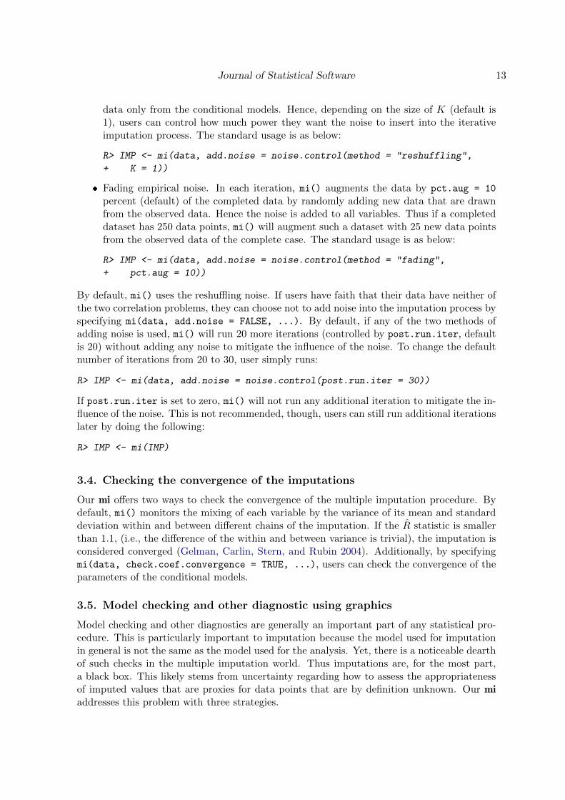
Fading empirical noise. In each iteration, mi() augments the data by pct.aug = 10

percent (default) of the completed data by randomly adding new data that are drawnfrom the observed data. Hence the noise is added to all variables. Thus if a completeddataset has 250 data points, mi() will augment such a dataset with 25 new data pointsfrom the observed data of the complete case. The standard usage is as below:

R> IMP <- mi(data, add.noise = noise.control(method = "fading",

+ pct.aug = 10))

By default, mi() uses the reshu✏ing noise. If users have faith that their data have neither ofthe two correlation problems, they can choose not to add noise into the imputation process byspecifying mi(data, add.noise = FALSE, ...). By default, if any of the two methods ofadding noise is used, mi() will run 20 more iterations (controlled by post.run.iter, defaultis 20) without adding any noise to mitigate the influence of the noise. To change the defaultnumber of iterations from 20 to 30, user simply runs:

R> IMP <- mi(data, add.noise = noise.control(post.run.iter = 30))

If post.run.iter is set to zero, mi() will not run any additional iteration to mitigate the in-fluence of the noise. This is not recommended, though, users can still run additional iterationslater by doing the following:

R> IMP <- mi(IMP)

3.4. Checking the convergence of the imputations

Our mi o↵ers two ways to check the convergence of the multiple imputation procedure. Bydefault, mi() monitors the mixing of each variable by the variance of its mean and standarddeviation within and between di↵erent chains of the imputation. If the R̂ statistic is smallerthan 1.1, (i.e., the di↵erence of the within and between variance is trivial), the imputation isconsidered converged (Gelman, Carlin, Stern, and Rubin 2004). Additionally, by specifyingmi(data, check.coef.convergence = TRUE, ...), users can check the convergence of theparameters of the conditional models.

3.5. Model checking and other diagnostic using graphics

Model checking and other diagnostics are generally an important part of any statistical pro-cedure. This is particularly important to imputation because the model used for imputationin general is not the same as the model used for the analysis. Yet, there is a noticeable dearthof such checks in the multiple imputation world. Thus imputations are, for the most part,a black box. This likely stems from uncertainty regarding how to assess the appropriatenessof imputed values that are proxies for data points that are by definition unknown. Our mi

addresses this problem with three strategies.


Imputations are typically generated using models, such as regressions or multivariatedistributions, which are fit to observed data. Thus the fit of these models to the observeddata can be checked (Gelman, Mechelen, Verbeke, Heitjan, and Meulders 2005) usingstandard graphical diagnostics.

Imputations can be checked using a standard of reasonability: the di↵erences betweenobserved and missing values, and the distribution of the completed data as a whole, canbe checked to see whether they make sense in the context of the problem being studied(Abayomi, Gelman, and Levy 2008).

So far, mi only implements the first two solutions with various plotting functions. We demon-strate the usages of these functions in Section 4.

4. Example

In this Section, we demonstrate some basic steps of mi with an example.

4.1. A study of HIV-positive people in New York City

The CHAIN dataset included in mi is a subset of the Community Health Advisory and Informa-tion Network (CHAIN) study. This study is a longitudinal cohort study of people living withHIV in New York City and is conducted by Columbia University School of Public Health(Messeri, Lee, Abramson, Aidala, Chiasson, and Jessop 2003). The CHAIN cohort was re-cruited in 1994 from a large number of medical care and social service agencies serving HIVin New York City. Cohort members were interviewed up to 8 times through 2002. A total of532 CHAIN participants completed at least one interview at either the 6th, 7th or 8th roundsof interview, and 508, 444, 388 interviews were completed respectively at rounds 6, 7 and 8(CHAIN 2009). For simplicity, our analysis here discards the time aspect of the dataset anduse only the 6th round of the survey. The dataset has 532 observations and has the following8 variables:

h39b.W1: Log of self reported viral load level, 0 represents undetectable level.

age.W1: The respondent’s age at time of interview.

c28.W1: The respondent’s family annual income. Values range from under USD 5, 000to USD 70, 000 or over.

pcs.W1: A continuous scale of physical health with a theoretical range between 0 and100 (better health is associated with higher scale values).

mcs37.W1: A dichotomous measure of poor mental health: 0 = No, 1 = Yes.

b05.W1: Ordered interval for the CD4 count (the indicator of how much damage HIVhas caused to the immune system).

haartadhere.W1: A three-level-ordered variable: 0 = not currently taking highly activeantiretroviral therapy (HAART), 1 = taking HAART nonadherent, 2 = taking HAARTadherent.


To use the data, users must first load the mi package:3

R> library("mi")

Loading required package: MASS

Loading required package: nnet

Loading required package: car

...

Loading required package: arm

Loading required package: Matrix

Loading required package: lattice

...

Loading required package: lme4

...

Loading required package: abind

mi (Version 0.09-13, built: 2011-2-15)

Then load the CHAIN dataset in the memory:

R> data("CHAIN")

4.2. Setup

The first thing to do is to set up the imputation. As with most statistical procedures, onemust start with some preliminary analysis to avoid trivial problems. When that is completed,two key steps must be done: choosing the conditional models and specifying the models.

Preliminary analysis is crucial in an iterative procedure such as multiple imputation that usesthe chain equation algorithm. Users do not want simple mistakes that arise in the early stagesto ruin the end result after a long iteration. In a small dataset, this may not be a seriousissue, but for a large dataset, this may be costly. There are problems which mi automaticallydetects. But there are problems that are not possible to detect automatically by mi. Forthose problems that are di�cult to detect, our mi will raise flags so that user can keep themin mind.

Display of missing data patterns

Users can get the glimpse of the data by looking at the missingness pattern.

R> missing.pattern.plot(CHAIN, clustered = FALSE)

Or simply type:

3The printout of the loaded information shows that mi depends upon on several R packages, including MASS

and nnet (Venables and Ripley 2002), car (Fox and Weisberg 2011), arm (Gelman et al. 2011), Matrix (Batesand Maechler 2011), lme4 (Bates, Maechler, and Bolker 2011), R2WinBUGS (Sturtz, Ligges, and Gelman2005), coda (Plummer, Best, Cowles, and Vines 2006) and abind (Plate and Heiberger 2011). In the last lineof the loaded information, R prints out the version number of mi. Users are welcome to report bugs or makesuggestions to us with the attached version number.


CHAIN

Index

h39b.W1

age.W1

c28.W1

pcs.W1

mcs37.W1

b05.W1

haartadhere.W1

CHAIN

Ordered by number of missing items

h39b.W1

b05.W1

c28.W1

age.W1

pcs.W1

mcs37.W1

haartadhere.W1

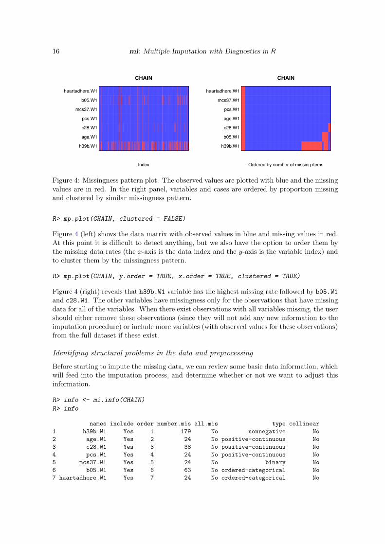
Figure 4: Missingness pattern plot. The observed values are plotted with blue and the missingvalues are in red. In the right panel, variables and cases are ordered by proportion missingand clustered by similar missingness pattern.

R> mp.plot(CHAIN, clustered = FALSE)

Figure 4 (left) shows the data matrix with observed values in blue and missing values in red.At this point it is di�cult to detect anything, but we also have the option to order them bythe missing data rates (the x-axis is the data index and the y-axis is the variable index) andto cluster them by the missingness pattern.

R> mp.plot(CHAIN, y.order = TRUE, x.order = TRUE, clustered = TRUE)

Figure 4 (right) reveals that h39b.W1 variable has the highest missing rate followed by b05.W1

and c28.W1. The other variables have missingness only for the observations that have missingdata for all of the variables. When there exist observations with all variables missing, the usershould either remove these observations (since they will not add any new information to theimputation procedure) or include more variables (with observed values for these observations)from the full dataset if these exist.

Identifying structural problems in the data and preprocessing

Before starting to impute the missing data, we can review some basic data information, whichwill feed into the imputation process, and determine whether or not we want to adjust thisinformation.

R> info <- mi.info(CHAIN)

R> info


1 h39b.W1 Yes 1 179 No nonnegative No

2 age.W1 Yes 2 24 No positive-continuous No

3 c28.W1 Yes 3 38 No positive-continuous No

4 pcs.W1 Yes 4 24 No positive-continuous No

5 mcs37.W1 Yes 5 24 No binary No

6 b05.W1 Yes 6 63 No ordered-categorical No

7 haartadhere.W1 Yes 7 24 No ordered-categorical No


By default, mi.info() prints out seven out of the fourteen categories of the mi.info matrix(see Section 2). We can see from this output that h39b.W1, age.W1, c28.W1, and pcs.W1

are variable types that need special treatment (see Section 3 for data preprocessing andtransformation).

So to address the variable types that mi.info() identifies as requiring special treatment,mi preprocesses the data via mi.preprocess() and may change the default judgement re-turned by typecase() (see Section 2 and Figure 2). mi.preprocess returns an S4 objectmi.preprocess that stores the transformed data in the slot data and the new mi.info objectin the slot mi.info.

R> CHAIN.new <- mi.preprocess(CHAIN)

R> attr(CHAIN.new, "mi.info")


1 h39b.W1.mi.log Yes 1 367 No log-continuous No

2 age.W1.mi.log Yes 2 24 No log-continuous No

3 c28.W1.mi.log Yes 3 38 No log-continuous No

4 pcs.W1.mi.log Yes 4 24 No log-continuous No

5 mcs37.W1 Yes 5 24 No binary No

6 b05.W1 Yes 6 63 No ordered-categorical No

7 haartadhere.W1 Yes 7 24 No ordered-categorical No

8 h39b.W1.mi.ind Yes 8 179 No binary No

The new information matrix shows that h39b.W1, age.W1, c28.W1, and pcs.W1 have beentransformed into new variables with di↵erent scales and types. Also, the transformed variableshave been attached with new su�xes.

Specifying the conditional models

mi() chooses the conditional models based on the variable types that are determined bytypecast() (see Section 2). By changing the variable types, mi() will choose di↵erent con-ditional models to fit the altered variables. For example, you can change the type of h39b.W1from nonnegative to continuous as:

R> info <- mi.info(CHAIN)

R> info


1 h39b.W1 Yes 1 179 No nonnegative No

...

R> info.upd <- update(info, "type", list("h39b.W1" = "continuous"))

R> info.upd


1 h39b.W1 Yes 1 179 No continuous No

...

By default, mi() assumes linearity between the outcomes and additive predictors.


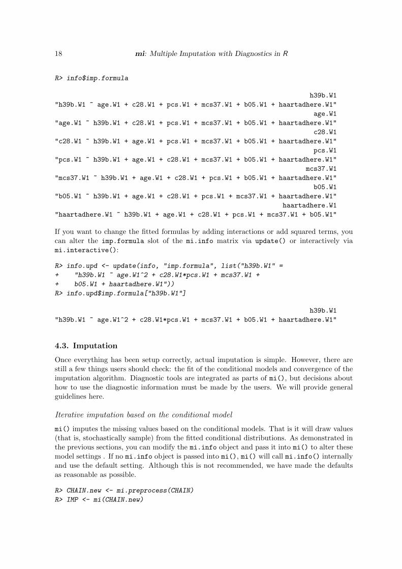
R> info$imp.formula

h39b.W1

"h39b.W1 ~ age.W1 + c28.W1 + pcs.W1 + mcs37.W1 + b05.W1 + haartadhere.W1"

age.W1

"age.W1 ~ h39b.W1 + c28.W1 + pcs.W1 + mcs37.W1 + b05.W1 + haartadhere.W1"

c28.W1

"c28.W1 ~ h39b.W1 + age.W1 + pcs.W1 + mcs37.W1 + b05.W1 + haartadhere.W1"

pcs.W1

"pcs.W1 ~ h39b.W1 + age.W1 + c28.W1 + mcs37.W1 + b05.W1 + haartadhere.W1"

mcs37.W1

"mcs37.W1 ~ h39b.W1 + age.W1 + c28.W1 + pcs.W1 + b05.W1 + haartadhere.W1"

b05.W1

"b05.W1 ~ h39b.W1 + age.W1 + c28.W1 + pcs.W1 + mcs37.W1 + haartadhere.W1"

haartadhere.W1

"haartadhere.W1 ~ h39b.W1 + age.W1 + c28.W1 + pcs.W1 + mcs37.W1 + b05.W1"

If you want to change the fitted formulas by adding interactions or add squared terms, youcan alter the imp.formula slot of the mi.info matrix via update() or interactively viami.interactive():

R> info.upd <- update(info, "imp.formula", list("h39b.W1" =

+ "h39b.W1 ~ age.W1^2 + c28.W1*pcs.W1 + mcs37.W1 +

+ b05.W1 + haartadhere.W1"))

R> info.upd$imp.formula["h39b.W1"]

h39b.W1

"h39b.W1 ~ age.W1^2 + c28.W1*pcs.W1 + mcs37.W1 + b05.W1 + haartadhere.W1"

4.3. Imputation

Once everything has been setup correctly, actual imputation is simple. However, there arestill a few things users should check: the fit of the conditional models and convergence of theimputation algorithm. Diagnostic tools are integrated as parts of mi(), but decisions abouthow to use the diagnostic information must be made by the users. We will provide generalguidelines here.

Iterative imputation based on the conditional model

mi() imputes the missing values based on the conditional models. That is it will draw values(that is, stochastically sample) from the fitted conditional distributions. As demonstrated inthe previous sections, you can modify the mi.info object and pass it into mi() to alter thesemodel settings . If no mi.info object is passed into mi(), mi() will call mi.info() internallyand use the default setting. Although this is not recommended, we have made the defaultsas reasonable as possible.

R> CHAIN.new <- mi.preprocess(CHAIN)

R> IMP <- mi(CHAIN.new)


Beginning Multiple Imputation ( Fri Jul 02 10:54:34 2010 ):

Iteration 1

Chain 1 : h39b.W1.mi.log* age.W1.mi.log* c28.W1.mi.log* pcs.W1.mi.log* mcs37.W1* b05.W1* haartadhere.W1* h39b.W1.mi.ind*



Iteration 2

Chain 1 : h39b.W1.mi.log age.W1.mi.log c28.W1.mi.log pcs.W1.mi.log* mcs37.W1* b05.W1 haartadhere.W1 h39b.W1.mi.ind

Chain 2 : h39b.W1.mi.log age.W1.mi.log* c28.W1.mi.log* pcs.W1.mi.log* mcs37.W1 b05.W1 haartadhere.W1* h39b.W1.mi.ind

Chain 3 : h39b.W1.mi.log age.W1.mi.log* c28.W1.mi.log pcs.W1.mi.log mcs37.W1 b05.W1 haartadhere.W1 h39b.W1.mi.ind*

...

Iteration 30

Chain 1 : h39b.W1.mi.log age.W1.mi.log c28.W1.mi.log pcs.W1.mi.log mcs37.W1* b05.W1 haartadhere.W1 h39b.W1.mi.ind

Chain 2 : h39b.W1.mi.log age.W1.mi.log c28.W1.mi.log pcs.W1.mi.log mcs37.W1 b05.W1 haartadhere.W1 h39b.W1.mi.ind

Chain 3 : h39b.W1.mi.log age.W1.mi.log c28.W1.mi.log pcs.W1.mi.log mcs37.W1* b05.W1 haartadhere.W1 h39b.W1.mi.ind

Reached the maximum iteration, mi did not converge ( Wed Feb 09 16:49:30 2011 )

Run 20 more iterations to mitigate the influence of the noise...

Beginning Multiple Imputation ( Wed Feb 09 16:49:30 2011 ):

Iteration 1




Iteration 2




...

Iteration 20




mi converged ( Wed Feb 09 16:50:06 2011 )

By default, mi() will perform reshu✏ing, and run 20 more iterations after the first mi() isfinished (add.noise = noise.control(K = 1, post.run.iter = 20)). The star symbolsattached to the variable names indicate that reshu✏ing is being implemented for that variablein that iteration. Before doing mi, if users want to use the mi() to transform the data, theycan transform the data with their own design or use mi.preprocess() to do the job. Here,we use mi.preprocess() to transform the data before we starting the imputation process.

There are other options to specify number of iterations (n.iter), how long mi() should run(max.minutes), whether or not mi should continue when it converged (run.past.convergence),etc (see Section 2 or type ?mi in the R console for details).

Checking the fit of conditional models and imputed values

If the fit of our imputation models to the observed data is poor, it is unlikely that we willimpute reasonable values for the missing values even our data are truly missing at random.We can check this fit through the binned residuals plot for the observed data and throughoverlaid histograms comparing observed and imputed data. Moreover, if the missing at ran-dom assumption is not appropriate we may be able to detect that by comparing imputedvalues to observed values based on what we know about the science of the phenomenon beingmeasured by the variables in our dataset. mi provides three di↵erent plots to visually inspectthe fit of the conditional models.

Imputation may take some time to run, depending on the size of the data. Thus we suggestthat users may want to check the fit of the conditional models (Gelman, Mechelen, Verbeke,Heitjan, and Meulders 2005; Abayomi, Gelman, and Levy 2008) by plotting the mi object(Figure 5) after a reasonable number of iterations rather than waiting for convergence. Fur-thermore, if working with a large sample size, it may also be helpful to diagnose the imputationprocedure for a random sample from the full sample.

R> plot(IMP)

The first plot displays histograms of the observed (in blue color), the imputed (in red color)and the completed (observed plus imputed, in black color) values. The second is a binned


Figure 5: Diagnostic plots for checking the fit of the conditional imputation models. To savepage space, only four out of the eight plots for each variable are displayed. The blue color isfor the observed value and the red color is for the imputed one. By default, these values areplotted against an index number. Plotting against a variable that contains more informationis a strongly recommended alternative. Fitted lowess curves are also plotted for the observeddata. A small amount of random noise (jittering) is added to the points so that they do notfall on top of each other.


80% interval for each chain R−hat

0

0

2

2

4

4

1 1.5 2+

1 1.5 2+

1 1.5 2+

1 1.5 2+

1 1.5 2+

1 1.5 2+

mean(h39b.W1.mi.log) ●●●

mean(age.W1.mi.log) ●●●

mean(c28.W1.mi.log) ●●●

mean(pcs.W1.mi.log) ●●●

mean(mcs37.W1) ●●●

mean(b05.W1) ●●●

mean(haartadhere.W1) ●●●

mean(h39b.W1.mi.ind) ●●●

sd(h39b.W1.mi.log) ●●●

sd(age.W1.mi.log) ●●●

sd(c28.W1.mi.log) ●●●

sd(pcs.W1.mi.log) ●●●

sd(mcs37.W1) ●●●

sd(b05.W1) ●●●

sd(haartadhere.W1) ●●●

sd(h39b.W1.mi.ind) ●●●

medians and 80% intervals

mean(h39b.W1.mi.log)

2.15

2.2

2.25

●

●

●

mean(age.W1.mi.log)

3.725

3.73

3.735●●

●

mean(c28.W1.mi.log)

1.021.031.041.051.06

●●

●

mean(pcs.W1.mi.log)

3.745

3.75

3.755

●

●

●

mean(mcs37.W1)

0.2650.27

0.2750.28

0.285

●●

●

mean(b05.W1)

3.55

3.6

3.65

●●●

mean(haartadhere.W1)

1.851.861.871.88

●

●

●

mean(h39b.W1.mi.ind)

0.460.480.50.52

●

●

●

sd(h39b.W1.mi.log)

0.180.190.20.210.22

●

●●

sd(age.W1.mi.log)

0.1960.1980.2

0.202

●●

●

sd(c28.W1.mi.log)

0.61

0.62

0.63

●

●

●

sd(pcs.W1.mi.log)

0.30.3050.31

0.315

●●●

sd(mcs37.W1)

0.44

0.445

0.45

●●

●

sd(b05.W1)

1.321.341.361.38

●●●

sd(haartadhere.W1)

0.860.8650.87

0.875

●●●

sd(h39b.W1.mi.ind)

0.4995

0.5

0.5005●●●

3 chains, each with 59 iterations (first 0 discarded)

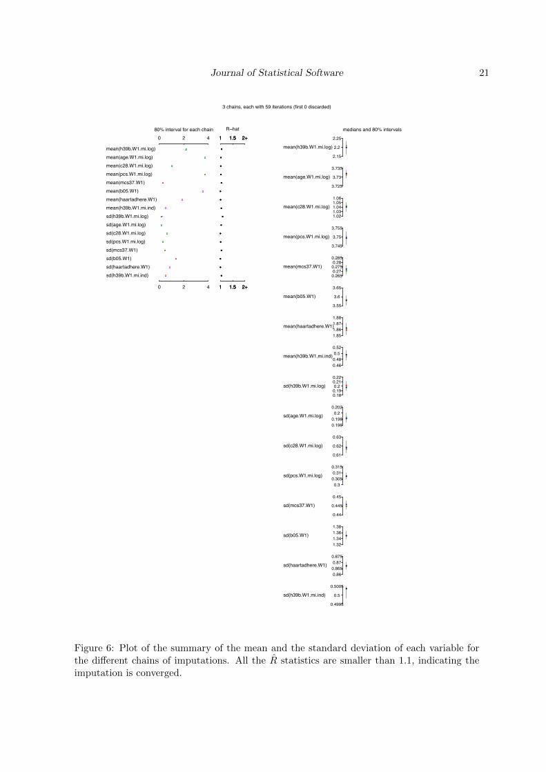
Figure 6: Plot of the summary of the mean and the standard deviation of each variable forthe di↵erent chains of imputations. All the R̂ statistics are smaller than 1.1, indicating theimputation is converged.


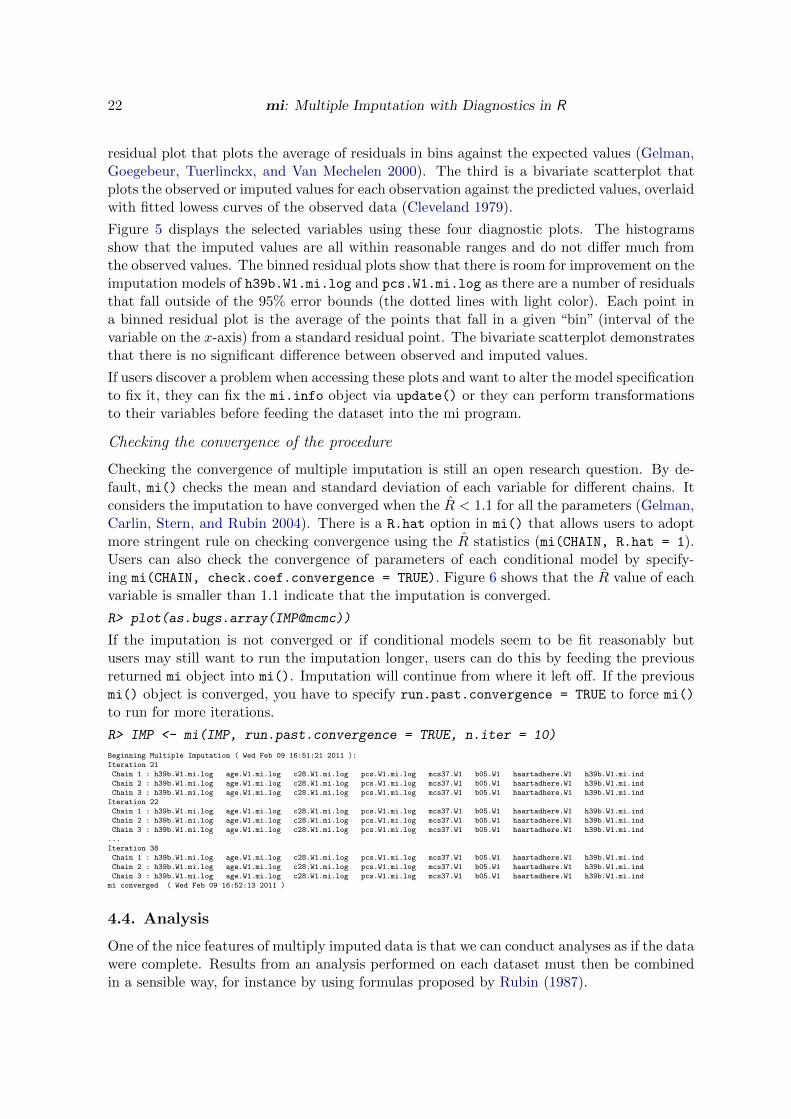
residual plot that plots the average of residuals in bins against the expected values (Gelman,Goegebeur, Tuerlinckx, and Van Mechelen 2000). The third is a bivariate scatterplot thatplots the observed or imputed values for each observation against the predicted values, overlaidwith fitted lowess curves of the observed data (Cleveland 1979).

Figure 5 displays the selected variables using these four diagnostic plots. The histogramsshow that the imputed values are all within reasonable ranges and do not di↵er much fromthe observed values. The binned residual plots show that there is room for improvement on theimputation models of h39b.W1.mi.log and pcs.W1.mi.log as there are a number of residualsthat fall outside of the 95% error bounds (the dotted lines with light color). Each point ina binned residual plot is the average of the points that fall in a given “bin” (interval of thevariable on the x-axis) from a standard residual point. The bivariate scatterplot demonstratesthat there is no significant di↵erence between observed and imputed values.

If users discover a problem when accessing these plots and want to alter the model specificationto fix it, they can fix the mi.info object via update() or they can perform transformationsto their variables before feeding the dataset into the mi program.

Checking the convergence of the procedure

Checking the convergence of multiple imputation is still an open research question. By de-fault, mi() checks the mean and standard deviation of each variable for di↵erent chains. Itconsiders the imputation to have converged when the R̂ < 1.1 for all the parameters (Gelman,Carlin, Stern, and Rubin 2004). There is a R.hat option in mi() that allows users to adoptmore stringent rule on checking convergence using the R̂ statistics (mi(CHAIN, R.hat = 1).Users can also check the convergence of parameters of each conditional model by specify-ing mi(CHAIN, check.coef.convergence = TRUE). Figure 6 shows that the R̂ value of eachvariable is smaller than 1.1 indicate that the imputation is converged.

R> plot(as.bugs.array(IMP@mcmc))

If the imputation is not converged or if conditional models seem to be fit reasonably butusers may still want to run the imputation longer, users can do this by feeding the previousreturned mi object into mi(). Imputation will continue from where it left o↵. If the previousmi() object is converged, you have to specify run.past.convergence = TRUE to force mi()

to run for more iterations.

R> IMP <- mi(IMP, run.past.convergence = TRUE, n.iter = 10)

Beginning Multiple Imputation ( Wed Feb 09 16:51:21 2011 ):

Iteration 21




Iteration 22




...

Iteration 38




mi converged ( Wed Feb 09 16:52:13 2011 )

4.4. Analysis

One of the nice features of multiply imputed data is that we can conduct analyses as if the datawere complete. Results from an analysis performed on each dataset must then be combinedin a sensible way, for instance by using formulas proposed by Rubin (1987).


Obtaining completed datasets

If the users prefer to perform separate data analyses for each dataset by themselves, theycan easily extract the completed datasets from the mi object via mi.completed(). This willreturn a list that contains multiple datasets.

R> IMP.dat.all <- mi.completed(IMP)

They can extract just one dataset from a specific chain of imputations via mi.data.frame().

R> IMP.dat <- mi.data.frame(IMP, m = 1)

mi also o↵ers an option to output these multiply imputed datasets into files. Currently, mi

only supports three data formats: csv, dta, and table. The default output data format iscsv.

R> write.mi(IMP)

The output files shall be stored under the working directory. The file names will bemidata1.csv, midata2.csv, midata3.csv, . . ., and so on.

Pooling the complete case analysis on multiply imputed datasets

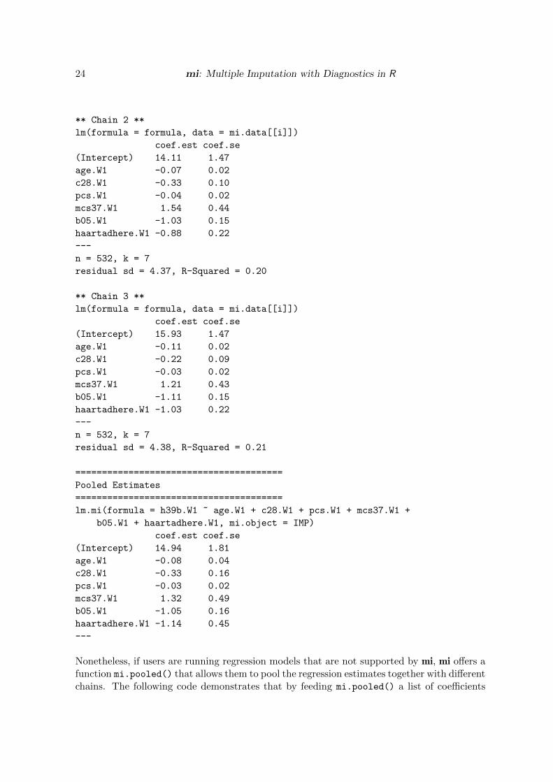
mi() facilitates the analysis process by providing functions that perform these separate anal-yses and then combine the separate estimates into one estimate and standard error. mi

currently o↵ers seven regression functions: lm.mi(), glm.mi(), polr.mi(), bayesglm.mi(),bayespolr.mi(), lmer.mi(), and glmer.mi().

R> fit <- lm.mi(h39b.W1 ~ age.W1 + c28.W1 + pcs.W1 + mcs37.W1 +

+ b05.W1 + haartadhere.W1, IMP)

R> display(fit)

=======================================

Separate Estimates for each Imputation

=======================================

** Chain 1 **

lm(formula = formula, data = mi.data[[i]])

coef.est coef.se

(Intercept) 14.78 1.46

age.W1 -0.06 0.02

c28.W1 -0.44 0.10

pcs.W1 -0.04 0.02

mcs37.W1 1.20 0.43

b05.W1 -0.99 0.14

haartadhere.W1 -1.52 0.22

---

n = 532, k = 7

residual sd = 4.36, R-Squared = 0.24


** Chain 2 **


coef.est coef.se


age.W1 -0.07 0.02

c28.W1 -0.33 0.10

pcs.W1 -0.04 0.02

mcs37.W1 1.54 0.44

b05.W1 -1.03 0.15


---

n = 532, k = 7


** Chain 3 **


coef.est coef.se


age.W1 -0.11 0.02

c28.W1 -0.22 0.09

pcs.W1 -0.03 0.02

mcs37.W1 1.21 0.43

b05.W1 -1.11 0.15


---

n = 532, k = 7


=======================================

Pooled Estimates

=======================================

lm.mi(formula = h39b.W1 ~ age.W1 + c28.W1 + pcs.W1 + mcs37.W1 +

b05.W1 + haartadhere.W1, mi.object = IMP)

coef.est coef.se


age.W1 -0.08 0.04

c28.W1 -0.33 0.16

pcs.W1 -0.03 0.02

mcs37.W1 1.32 0.49

b05.W1 -1.05 0.16


---

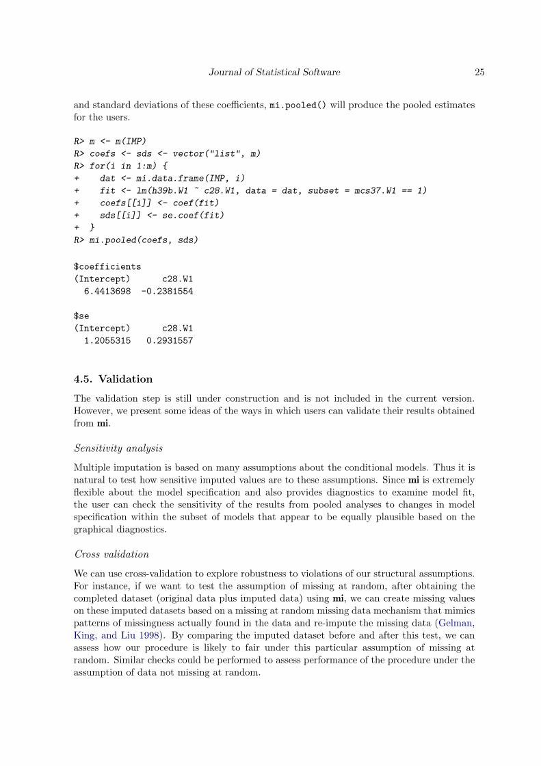
Nonetheless, if users are running regression models that are not supported by mi, mi o↵ers afunction mi.pooled() that allows them to pool the regression estimates together with di↵erentchains. The following code demonstrates that by feeding mi.pooled() a list of coe�cients


and standard deviations of these coe�cients, mi.pooled() will produce the pooled estimatesfor the users.

R> m <- m(IMP)

R> coefs <- sds <- vector("list", m)

R> for(i in 1:m) {

+ dat <- mi.data.frame(IMP, i)

+ fit <- lm(h39b.W1 ~ c28.W1, data = dat, subset = mcs37.W1 == 1)

+ coefs[[i]] <- coef(fit)

+ sds[[i]] <- se.coef(fit)

+ }

R> mi.pooled(coefs, sds)

$coefficients

(Intercept) c28.W1

6.4413698 -0.2381554

$se

(Intercept) c28.W1

1.2055315 0.2931557

4.5. Validation

The validation step is still under construction and is not included in the current version.However, we present some ideas of the ways in which users can validate their results obtainedfrom mi.

Sensitivity analysis

Multiple imputation is based on many assumptions about the conditional models. Thus it isnatural to test how sensitive imputed values are to these assumptions. Since mi is extremelyflexible about the model specification and also provides diagnostics to examine model fit,the user can check the sensitivity of the results from pooled analyses to changes in modelspecification within the subset of models that appear to be equally plausible based on thegraphical diagnostics.

Cross validation

We can use cross-validation to explore robustness to violations of our structural assumptions.For instance, if we want to test the assumption of missing at random, after obtaining thecompleted dataset (original data plus imputed data) using mi, we can create missing valueson these imputed datasets based on a missing at random missing data mechanism that mimicspatterns of missingness actually found in the data and re-impute the missing data (Gelman,King, and Liu 1998). By comparing the imputed dataset before and after this test, we canassess how our procedure is likely to fair under this particular assumption of missing atrandom. Similar checks could be performed to assess performance of the procedure under theassumption of data not missing at random.


Compatibility check

We will use graphical diagnostics to assess the extent to which our conditional models fail toprovide consistent information about the underlying joint distribution of the data and explorethe extent to which such incompatibility might impact our results.

4.6. Interactive interface

mi has an interactive program where users do not have to type commands to perform multipleimputation. By calling mi.iteractive() and giving it the data to be imputed, it will walkthe users through all the necessary settings and steps as discussed in the previous sections.

R> data("CHAIN")

R> IMP <- mi.interactive("CHAIN")

-----------------------------------

creating information matrix:

-----------------------------------

done

-----------------------------------

Would you like to:

-----------------------------------

1: look at current setting

2: proceed to mi with current setting

3: change current setting

Selection:

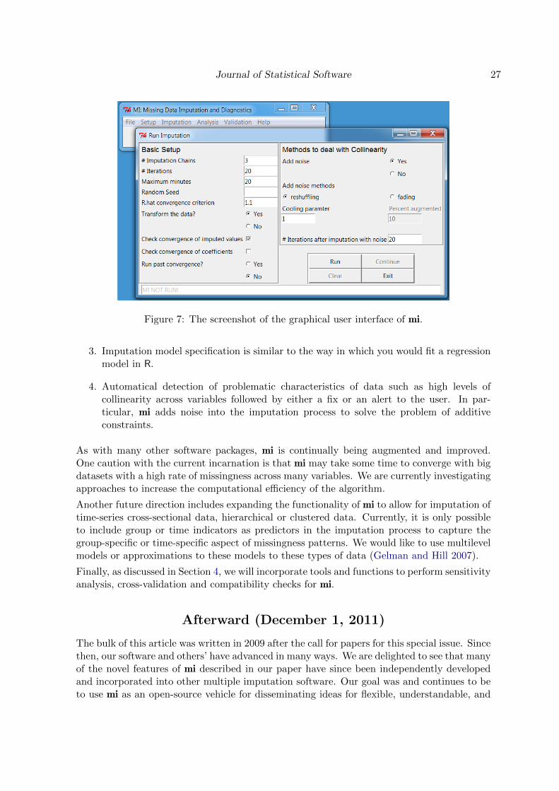
Additionally, migui (Lee and Su 2010) o↵ers a graphical user interface (GUI) of mi whereusers can do multiple imputation by clicking buttons. To call up the GUI, simply type thefollowings in the R console:

R> library("migui")

R> migui()

5. Conclusions and future plans

The major goal of mi is to make multiple imputation transparent and easy to use for theusers. Here are four characteristics of the package that we believe are particularly valuable.

1. Graphical diagnostics of imputation models and convergence of the imputation process.

2. Use of Bayesian versions of regression models to handle the issue of separation.


Figure 7: The screenshot of the graphical user interface of mi.

3. Imputation model specification is similar to the way in which you would fit a regressionmodel in R.

4. Automatical detection of problematic characteristics of data such as high levels ofcollinearity across variables followed by either a fix or an alert to the user. In par-ticular, mi adds noise into the imputation process to solve the problem of additiveconstraints.

As with many other software packages, mi is continually being augmented and improved.One caution with the current incarnation is that mi may take some time to converge with bigdatasets with a high rate of missingness across many variables. We are currently investigatingapproaches to increase the computational e�ciency of the algorithm.

Another future direction includes expanding the functionality of mi to allow for imputation oftime-series cross-sectional data, hierarchical or clustered data. Currently, it is only possibleto include group or time indicators as predictors in the imputation process to capture thegroup-specific or time-specific aspect of missingness patterns. We would like to use multilevelmodels or approximations to these models to these types of data (Gelman and Hill 2007).

Finally, as discussed in Section 4, we will incorporate tools and functions to perform sensitivityanalysis, cross-validation and compatibility checks for mi.

Afterward (December 1, 2011)

The bulk of this article was written in 2009 after the call for papers for this special issue. Sincethen, our software and others’ have advanced in many ways. We are delighted to see that manyof the novel features of mi described in our paper have since been independently developedand incorporated into other multiple imputation software. Our goal was and continues to beto use mi as an open-source vehicle for disseminating ideas for flexible, understandable, and


checkable missing data imputation. In particular, we are looking forward to seeing one ofthe important features of mi – model checking and cross validation after imputation – to beincorporated in other software, just as we will continue to take advantage of developmentselsewhere in improving our programs. The synergy available from open-source software shouldbe a general benefit.

Acknowledgments

We thank Peter Messeri for the CHAIN example, Maria Grazia Pittau for helpful discussionsand her early works on mi, Benjamin Goodrich for his current e↵orts on making mi better, theUS Nation Science Foundation, National Institutes of Health, Institute of Education Sciences,and the Wang Xuelian Foundation for partial support of this research.

References

Abayomi K, Gelman A, Levy M (2008). “Diagnostics for Multivariate Imputations.” Journalof the Royal Statistical Society C, 57(3), 273–291.

Bates D, Maechler M (2011). Matrix: Sparse and Dense Matrix Classes and Methods.R package version 1.0-1, URL http://CRAN.R-project.org/package=Matrix.

Bates D, Maechler M, Bolker B (2011). lme4: Linear Mixed-E↵ects Models Using S4 Classes.R package version 0.999375-42, URL http://CRAN.R-project.org/package=lme4.

Buuren SV, Groothuis-Oudshoorn K (2011). “mice: Multivariate Imputation by ChainedEquations in R.” Journal of Statistical Software, 45(3), 1–67. URL http://www.

jstatsoft.org/v45/i03/.

CHAIN (2009). “NY HIV Data CHAIN.” URL http://www.nyhiv.org/data_chain.html.

Cleveland WS (1979). “Robust Locally Weighted Regression and Smoothing Scatterplots.”Journal of the American Statistical Association, 74(368), 829–836.

Fay RE (1996). “Alternative Paradigms for the Analysis of Imputed Survey Data.” Journalof the American Statistical Association, 91(434), 490–498.

Fox J, Weisberg S (2011). car: Companion to Applied Regression. R package version 2.0-11,URL http://CRAN.R-project.org/package=car.

Gelman A, Carlin JB, Stern HS, Rubin DB (2004). Bayesian Data Analysis. 2nd edition.Chapman & Hall/CRC, Boca Raton, Fl.

Gelman A, Goegebeur Y, Tuerlinckx F, Van Mechelen I (2000). “Diagnostic Checks forDiscrete Data Regression Models Using Posterior Predictive Simulations.” Journal of theRoyal Statistical Society C, 49(2), 247–268.

Gelman A, Hill J (2007). Data Analysis Using Regression and Multilevel/Hierarchical Models.Cambridge University Press, UK.

http://CRAN.R-project.org/package=Matrix

http://CRAN.R-project.org/package=lme4

http://www.jstatsoft.org/v45/i03/


http://www.nyhiv.org/data_chain.html

http://CRAN.R-project.org/package=car


Gelman A, Jakulin A, Pittau MG, Su YS (2008). “A Weakly Informative Default PriorDistribution for Logistic and Other Regression Models.” The Annals of Applied Statistics,2(4), 1360–1383.

Gelman A, King G, Liu C (1998). “Not Asked and Not Answered: Multiple Imputation forMultiple Surveys.” Journal of the American Statistical Association, 93(443), 846–857.

Gelman A, Mechelen IV, Verbeke G, Heitjan DF, Meulders M (2005). “Multiple Imputationfor Model Checking: Completed-Data Plots with Missing and Latent Data.” Biometrics,61(1), 74–85.

Gelman A, Rubin DB (1992). “Inference from Iterative Simulation Using Multiple Sequences.”Statistical Science, 7(4), 457–472.

Gelman A, Su YS, Yajima M, Hill J, Pittau MG, Kerman J, Zheng T (2011). arm: DataAnalysis Using Regression and Multilevel/Hierarchical Models. R package version 1.4-13,URL http://CRAN.R-project.org/package=arm.

Heitjan DF, Little RJA (1991). “Multiple Imputation for the Fatal Accident Reporting Sys-tem.” Journal of the Royal Statistical Society C, 40(1), 13–29.

Lee D, Su YS (2010). migui: Graphical User Interface of the mi Package. R packageversion 0.00-08, URL http://CRAN.R-project.org/package=migui.

Little RJA, Rubin DB (2002). Statistical Analysis with Missing Data. 2nd edition. JohnWiley & Sons, Hoboken.

Meng XL (1994). “Multiple-Imputation Inferences with Uncongenial Sources of Input.” Sta-tistical Science, 9(4), 538–558.

Messeri P, Lee G, Abramson DM, Aidala A, Chiasson MA, Jessop DJ (2003). “AntiretroviralTherapy and Declining AIDS Mortality in New York City.” Medical Care, 41(4), 512–521.

Plate T, Heiberger R (2011). abind: Combine Multi-Dimensional Arrays. R package ver-sion 1.3-0, URL http://CRAN.R-project.org/package=abind.

Plummer M, Best N, Cowles K, Vines K (2006). “coda: Convergence Diagnosis and Out-put Analysis for MCMC.” R News, 6(1), 7–11. URL http://CRAN.R-project.org/doc/

Rnews/.

Raghunathan TE, Lepkowski JM, Van Hoewyk J, Solenberger P (2001). “A MultivariateTechnique for Multiply Imputing Missing Values Using a Sequence of Regression Models.”Survey Methodology, 27(1), 85–95.

R Development Core Team (2011). R: A Language and Environment for Statistical Computing.R Foundation for Statistical Computing, Vienna, Austria. ISBN 3-900051-07-0, URL http:

//www.R-project.org/.

Robins JM, Wang N (2000). “Inference for Imputation Estimators.” Biometrika, 87(1), 113–124.

Rubin DB (1987). Multiple Imputation for Nonresponse in Surveys. John Wiley & Sons, NewYork.

http://CRAN.R-project.org/package=arm

http://CRAN.R-project.org/package=migui

http://CRAN.R-project.org/package=abind

http://CRAN.R-project.org/doc/Rnews/

http://CRAN.R-project.org/doc/Rnews/

http://www.R-project.org/

http://www.R-project.org/


Schenker N, Taylor JMG (1996). “Partially Parametric Techniques for Multiple Imputation.”Computational Statistics & Data Analysis, 22(4), 425–446.

Sturtz S, Ligges U, Gelman A (2005). “R2WinBUGS: A Package for Running WinBUGS

from R.” Journal of Statistical Software, 12(3), 1–16. URL http://www.jstatsoft.org/

v12/i03/.

Venables WN, Ripley BD (2002). Modern Applied Statistics with S. 4th edition. Springer-Verlag, New York.

A�liation:

Yu-Sung SuDepartment of Political ScienceSchool of Humanities and Social SciencesTsinghua UniversityRoom 153 Minzhai, Qinghua Yuan, Haidian DistrictBeijing, 100084, ChinaE-mail: [email protected]

Andrew GelmanDepartment of StatisticsColumbia University1255 Amsterdam AvenueNew York, NY 10027, United States of AmericaE-mail: [email protected]: http://www.stat.columbia.edu/~gelman/

Jennifer HillDepartment of Humanities and Social SciencesSteinhardt School of Culture, Education and Human DevelopmentNew York University246 Greene StreetNew York, NY 10003, United States of AmericaE-mail: [email protected]

Masanao YajimaDepartment of StatisticsUniversity of California, Los Angeles9407 Boelter Hall



mailto:[email protected]


http://www.stat.columbia.edu/~gelman/



Los Angeles, CA 90095-1554, United States of AmericaE-mail: [email protected]: http://www.stat.ucla.edu/~yajima/

Journal of Statistical Software http://www.jstatsoft.org/

published by the American Statistical Association http://www.amstat.org/

Volume 45, Issue 2 Submitted: 2009-06-15December 2011 Accepted: 2011-05-30


http://www.stat.ucla.edu/~yajima/

http://www.jstatsoft.org/

http://www.amstat.org/

multiple imputation with diagnostics (mi) in r: opening ...gelman/research/published/mipaper.pdf ·...

Documents