Multiple Time-Scales in Classical and Quantum-ClassicalMolecular DynamicsSebastian Reich�October 1, 1998AbstractThe existence of multiple time scales in molecular dynamics poses interesting and challengingquestions from an analytical as well as from a numerical point of view. In this paper, we considersimpli�ed models with two essential time scales and describe how these two time scales inter-act. The discussion focuses on classical molecular dynamics (CMD) with fast bond stretchingand bending modes and the, so called, quantum-classical molecular dynamics (QCMD) modelwhere the quantum part provides the highly-oscillatory solution components. The analytic res-ults on the averaging over fast degrees of motion will also shed new light on the appropriateimplementation of multiple-time-stepping (MTS) algorithms for CMD and QCMD.1 IntroductionClassical molecular dynamics (CMD) [1] leads to Newtonian equations of motion with fast bondstretching and bending modes and a relatively slow motion in the remaining degrees of freedom.For numerical integration, the Verlet method [43] is typically used with a step-size that resolves thefast bond stretching/bending modes. However, often one is interested in the computation of slowlyvarying quantities and/or time averages and a method such as Verlet can quickly become ine�cientfor long time simulations.Various approaches have been suggested to improve the classical Verlet method. Among theseare (i) methods based on the explicit elimination of the fast bond stretching/bending modes andthe subsequent integration of the corresponding constrained equations of motion by the SHAKE orRATTLE method [2, 37] and (ii) reversible multiple time stepping (MTS) methods [7, 23, 42] thatuse di�erent time steps for the fast and slow degrees of freedom.In appropriate (local) coordinates, the fast bond stretching and bending modes can be reduced toweakly coupled harmonic oscillators whose frequency depends on the slow modes. This dependenceleads to a coupling of the slow and fast modes which, in general, implies that the fast degrees ofmotion cannot be removed from the model without changing its long time dynamics [36, 41, 32, 14,11]. It seems that in those situations only methods based on the idea of MTS can and should beused for enhanced classical molecular dynamics. However, one has to be careful. Straightforwardapplication of a MTS method may lead to wrong results or to unstable computations [7, 9]. Thisfact is brie y discussed in x2. An improved approach to multiple time stepping has been suggestedby Garc�ia-Archilla, Sanz-Serna & Skeel in [19]. In x5, we consider a variant of this approach[34, 26] that is particularly suited for the multiple time scale integration of classical moleculardynamics (CMD).In recent years, the combination of quantum and classical molecular dynamics has become im-portant. In this paper, we focus on the, so called, quantum-classical molecular dynamics (QCMD)model [21, 20, 6, 12, 13] where most of the molecular system is described by classical Newtonianequations of motion while a small but important part is modeled by a time-varying Schr�odingerequation (see x3). Again the fast quantum degrees of freedom and the slow classical degrees offreedom are tightly coupled. In fact, the e�ect of this coupling on the (slow) classical degrees offreedom, which is linked to the Born-Oppenheimer approximation [13], is easier to understand than�Department of Mathematics and Statistics, University of Surrey, Guildford, Surrey GU2 5XH, UK, E-mail:s.reich@surrey.ac.uk 1

the corresponding coupling e�ects in classical molecular dynamics. However, as we will show inx4, classical molecular dynamics can be transformed to a system resembling the QCMD model andtheoretical results derived for the QCMD model can also be applied to classical molecular dynamics.This is con�rmed by the numerical simulation of a simple test problem.Because of the importance of the QCMD model, we also discuss MTS methods for QCMD[39, 30, 31]. Here it is crucial to observe that the method has to be implemented in an appropriateway and that some of the straightforward implementations can lead to erroneous numerical resultsin the (slow) classical degrees of freedom [24, 30, 31]. This aspect is discussed in x6.2 Classical MD and Multiple-Time-SteppingThe atomic motion of a molecular system, consisting ofN atoms, is typically described by Newtonianequations of motion of the form_q = M�1p; (1)_p = �rqV(q)� mXi=1Gi(q)T kiigi(q) (2)where q 2 R3N is the vector of all atomic positions, p 2 R3N the vector of the correspondingmomenta, M 2 R3N�3N the diagonal mass matrix, V(q) the potential energy except for the termscorresponding to bond stretching and bending which are described by the second term on the lefthand side of equation (2). Here the functions fgigi=1;::: ;m can either stand for gi(q) = r� r0 (bondstretching) or gi(q) = � � �0 (bond angle bending). In either case, Gi(q) 2 R3N denotes theJacobian of gi(q) and kii the force constant. For compactness of notation, we collect the functionsfgig in the vector-valued function g, the force constants fkiig in the diagonal matrix K 2 Rm�m,and the Jacobians fGi(q)g in the matrix G(q) 2 Rm�3N . This gives rise to the equations_q = M�1p; (3)_p = �rqV(q)�G(q)TKg(q): (4)The total energy H = 12pTM�1p+ V(q) + 12g(q)TKg(q)is a conserved quantity (�rst integral) along solutions of (3)-(4).Let us denote the potential energy of the system by U(q), i.e.U(q) := V(q) + 12g(q)TKg(q);and the kinetic energy by T (p). Then the Verlet method [43] can be considered as a compositionmethod [40] based on the exact solution operators of the two systems_q = rpT (p) = M�1p;_p = 0and _q = 0;_p = �rqU(q):Let us denote these solution operators by exp(tLT ) and exp(tLU ), respectively. Then one step ofthe Verlet method with a step-size �t is equivalent to the concatenationexp(�t2 LU ) � exp(�tLT ) � exp(�t2 LU ):Since each solution operator is volume preserving (and even symplectic), the Verlet method is volumepreserving (symplectic) [40]. Furthermore, the method conserves linear and angular momentum andthe time-reversibility of the Newtonian equations of motion.2

The Verlet method becomes ine�cient if the evaluation of the force �eld is expensive due tolong-range interactions. To enhance the classical Verlet method, a symplectic and time-reversiblemultiple-time-stepping (MTS) method was suggested in [7, 23, 42]. The idea of this MTS method isamazingly simple: We split the total potential energy U into two terms U1 and U2 with U1 containingall the short range interactions (in particular the bond stretching/bending modes). Then one stepof a MTS scheme with macro step-size �t = j�t, j � 1, reads1exp(�t2 LU2) � 2664exp(�t2 LU1) � exp(�tLT ) � exp(�t2 LU1)| {z }j times 3775 � exp(�t2 LU2): (5)This method has the same conservation properties as Verlet, but it is potentially more e�cient sincethe long range forces have to computed less frequently.Although the idea of (5) is simple, the method has some drawbacks. For certain values ofthe macro step-size �t, the method can become unstable (meaning a systematic increase in totalenergy) due to resonance/sampling phenomena [7, 9]. Even if there is no systematic increase inthe total energy, the numerical results can be qualitatively di�erent from those obtained from thestandard Verlet method. This e�ect does not occur for systems with strong bond bending/stretchingpotentials. But it can be observed for systems with very light particles if the splitting of theHamiltonian is not done properly. We will also encounter this problem when discussing MTSmethods for the QCMD model.Example 1. We take two harmonic oscillators Hx = (px)2=2+(qx)2=2 and Hy = (py)2=(2�2)+(qy)2=2, one of whichhas a very small \mass" m = �2, �! 0, coupled by a quadratic potential W = qxqy:H = 12 (px)2 + ��22 (py)2 + 12 (qx)2 + 12(qy)2 + qxqy:The equations of motion are _qx = px;_px = �qx � qy;_qy = ��2py;_py = �qy � qx:The last two equations describe a highly oscillatory motion about the \equilibrium" (�qx; 0). If this solution is usedin the second equation to time-average over the rapidly oscillating force termF (t) = �qx � qy(t);we obtain the averaged force hF i � 0. Thus, the \slow" dynamics in the variable (qx; px) is approximately given bythe equations _qx = px;_px = 0:A MTS scheme can be obtained via the splittingT = 12(px)2 + ��22 (py)2;U1 = 12(qy)2;and U2 = 12(qx)2 + qxqy:We assume that the step-size �t < � in (5) is chosen small enough such that the equations of motion corresponding tothe Hamiltonian T +U1 are solved \exactly". Next we de�ne the macro step-size �t such that the solutions to T +U1satisfy qy(�t) � qy(0) and py(�t) � py(0), i.e. �t � k�=(2�), k � 1. Thus, instead of sampling a highly oscillatorysolution, we obtain a �ctitious \constant" solution which, when plugged into the numerical approximation of_px = �qx � qy(t) = F (t)leads, in general, to a qualitatively wrong approximation of the averaged force hF i. This problem does not occur ifthe splitting U1 = 12(qy)2 + qxqy1See Fig. 3 in x5 for a more explicit formulation of (5).3

and U2 = 12(qx)2is used. �An alternative to the MTS scheme (5) is to replace the Verlet discretization of T (p) +U1(q) in theinner loop of (5) by one step with an implicit method (such as the implicit midpoint rule [40]) andstep-size �t = �t. However, in addition to the resonance problems of the MTS method (5) [28], onealso, in general, encounters an exponential instability unless the step-size �t is chosen su�cientlysmall [4]. Thus such an approach seems inappropriate for CMD simulations.3 Quantum-Classical Molecular Dynamics3.1 The QCMD ModelVarious extensions of classical mechanics to also include quantum e�ects have been introduced in theliterature. Here we consider the so-called quantum-classical molecular dynamics (QCMD) model.In the QCMD model (see [21, 20, 6, 12, 13] and references therein), most atoms are described byclassical mechanics, but an important small portion of the system by quantum mechanics. Thisleads to a coupled system of Newtonian and Schr�odinger equations.For ease of presentation, we consider the case of just one quantum degree of freedom with spatialcoordinate x and mass m and N classical particles with coordinates q 2 R3N and diagonal massmatrixM 2 R3N�3N . Upon denoting the interaction potential by V (x; q), we obtain the followingequations of motion for the QCMD model:_ = � i~H(q) ;_q = M�1p ;_p = �h ;rqH(q) i �rqU(q)with U(q) the purely classical potential energy and H(q) the quantum Hamiltonian operator typic-ally given by H(q) = T + V (x; q); T = � ~22m�x:In the sequel, we assume that the quantum subsystem has been truncated to a �nite-dimensionalsystem by an appropriate spatial discretization and a corresponding representation of the wavefunction by a complex-valued vector 2 Cd. The discretized quantum operators T; V and H aredenoted by T 2 Cd�d, V (q) 2 Cd�d and H(q) 2 Cd�d, respectively.The total energy of the systemH = pTM�1p2 + h ;H(q) i+ U(q) (6)is a conserved quantity of the QCMD model. Hereh ;H(q) i := � TH(q) and � denotes the complex conjugate of . Another conserved quantity is the norm of the vector , i.e., h ; i = const. due to the unitary propagation of the quantum part.In the context of this paper, an important conservation property of the QCMD model is relatedto its Hamiltonian structure which implies the symplecticness of the solution operator [3]. There aredi�erent ways to consider the QCMD model as a Hamiltonian system with Hamiltonian (6). Herewe basically2 follow the presentation given in [12, 38]: We decompose the complex-valued vector into its real and imaginary part, i.e., = 1p2(q + ip ) : (7)2We use a di�erent scaling in (7) which leads to the scaled canonical structure (8) of phase space.4

Then, the equations of motion can be derived from the scaled Lie-Poisson bracketfF;Gg = ~�1fF;Ggq ;p + fF;Ggq;p; (8)i.e., _f = ff;Hgdescribes the time evolution of a function f under the Hamiltonian H. The brackets fF;Ggq ;p andfF;Ggq;p in (8) stand for the canonical bracket of classical mechanics [3]. For example, fF;Ggq;p =[rqF ]TrpG� [rpF ]TrqG.3.2 The Limit Behavior of the QCMD ModelIt is of interest to consider the limit3 ~! 0 for a �xed energy function (6). As explicitly shown byBornemann & Sch�utte in [13, 15] using homogenization techniques, the QCMD model reduces tothe Born-Oppenheimer approximation if the symmetric matrix H(q) can be smoothly diagonalizedand its (real) eigenvalues fEi(q(t))gi=1;::: ;d are pairwise di�erent. This implies that the populationsj�i(t)j2, i = 1; : : : ; k, corresponding to the eigenvalues Ei(q(t))) of the operator H(q) becomeadiabatic invariants. Without going through a detailed analysis, this can be seen from the followingaveraging argument. Let us assume that there is a matrix valued function Q(q) 2 Rd�d such that(i) Q(q)TQ(q) = I and (ii) E(q) := Q(q)H(q)Q(q)T is diagonal. For simplicity, we consider onlyone classical degree of freedom, i.e. (q;p) = (q; p) 2 R2. Next we introduce the new vector� := Q(q) 2 Cdand obtain the transformed QCMD equations of motion_� = � i~E(q)� +M�1pA(q)� ; (9)_q = M�1p ; (10)_p = �h�;Q(q)rqH(q)Q(q)T �i � rqU(q) (11)with the skew-symmetric matrix A(q) := rqQ(q)Q(q)T . Note that M�1pA(q) = _Q(q)Q(q)T . Thefast motion is given by the diagonalized time-dependent Schr�odinger equation_� = � i~E(q)� (12)and the Hellmann-Feynman force FHF [12], acting on the classical particles, can be written asFHF = �h�;Q(q)rqH(q)Q(q)T�i = �h�;rqE(q)�i+ h�; [A(q)E(q)]�i: (13)with the matrix commutator [A(q);E(q)] = A(q)E(q)�E(q)A(q):We call FBO = �h�;rqE(q)�i (14)the Born-Oppenheimer part of the Hellmann-Feynman force (13).If all (real) elements of the diagonal matrix E(q) are di�erent, then the quantum adiabatictheorem [17, 10] implies that the transformed \wave" vector �(t) follows the solutions of the reducedsystem (12) and the motion in the classical degrees of freedom is obtained by time-averaging theHellmann-Feynman force (13) over the highly oscillatory solutions4 �(t) of (12). For this, it is3One should really consider the limitM !1, i.e., should increase the mass of the classical particles. But this isequivalent, after an appropriate rescaling of time, to taking the limit ~! 0.4The average is taken over a period of time T such that (i) q(t) � const. and (ii) the Schr�odinger equation (12)undergoes many oscillations. For example, T � p~ as ~! 0.5

crucial to observe that the matrix commutator [A(q)E(q)] has zero diagonal entries and, thus, thetime-average of h�(t); [A(q)E(q)]�(t)i is approximately zero. Thus we obtain the averaged system_� = � i~E(q)�;_q = M�1p;_p = �h�;rqE(q)�i � rqU(q):Since E(q) is diagonal, the entries �i(t) 2 C, i = 1; : : : ; d, of the vector �(t) satisfy j�i(t)j2 = const.and _q = M�1p;_p = �Xi j�ij2rqEii(q)�rqU(q):These equations are known as the Born-Oppenheimer approximation for the classical coordinate[16].If eigenvalues of the matrix E(q) cross, then j�i(t)j2 6= const., in general, and the Born-Oppenheimer approximation breaks down. In this case, the full QCMD model has to be solved.Note that the crossing of eigenvalues cannot be avoided in general.Example 2. Let us consider a simple toy problem with two fast modes and one slow mode:H(q) = � q cos2 q + (1� q) sin2 q (1� 2q) sin q cos q(1� 2q) sin q cos q q sin2 q + (1 � q) cos2 q � ;= � cos q sin q� sin q cos q � � q 00 1� q � � cos q � sin qsin q cos q �and H = 12p2 + 12 q2 + h ;H(q) i;q; p 2 R, 2 C2. Note that Q(q) = � cos q � sin qsin q cos q � ;E(q) = � q 00 1� q � ;and A = � 0 �11 0 � :Thus the transformed equations of motion are_� = � i~E(q)� + pA�;_q = p;_p = �q � h�;B�i+ h�;C(q)�iwith B = � 1 00 �1 �and C(q) = [A;E(q)] = � 0 2q � 12q � 1 0 � :The Hellmann-Feynman force (13) is given byFHF = �h�;B�i+ h�;C(q)�i: (15)Unless q � 0:5 (resonance point), the equations can be averaged and we obtain the Born-Oppenheimer system_� = � i~E(q)�;_q = M�1p;_p = �q � h�;B�i:Numerical results are presented in x6. �6

4 Multiple Time Scales in Classical MD4.1 A Classical MD ModelWe now come back to the CMD model of x2. In particular, we consider a conservative system withHamiltonian HK = 12pTM�1p+ V(q) + K2 g(q)T g(q) (16)where V : Rn ! R and g : Rn ! Rm, m < n, are nonnegative functions, M 2 Rn�n is a diagonalmass matrix, and K � 1 is a parameter5. We are interested in the limit K ! 1 and solutionswith energy HK � c for all K su�ciently large; c > 0 some given constant. This implies that eachcomponent gi(q), i = 1; : : : ;m, of the vector valued function g satis�esgi(q) �r2cKand, for K !1, suggests to replace the equations of motion_q = M�1p;_p = �rqV(q)�KG(q)T g(q);G(q) 2 Rm�n the Jacobian of g(q), by the constrained system_q = M�1p; (17)_p = �rqV(q)�G(q)T�; (18)0 = g(q): (19)We assume throughout the paper that the m�m matrix G(q)M�1G(q)T is invertible.The constrained system can be integrated numerically using the SHAKE or RATTLE method[2, 37] which are basically equivalent [27] and lead to a modi�ed Verlet method of typeqn+1 = qn +�tM�1pn+1=2;pn+1=2 = pn � �t2 rqV(qn)��tG(qn)T�n;pn+1 = pn+1=2 � �t2 rqV(qn+1);0 = g(qn+1):Although this approach is very appealing, the constrained system does not, in general, re ect thecorrect limit behavior of the unconstrained system for K � 1. There are basically two problems:� Even in the limit K ! 1, solutions of (16) do not, in general, reduce to solutions of theconstrained system (17)-(19). This is due to a coupling of the fast oscillations to the slowlyvarying solution components. This coupling gives rise to an additional (correcting) force termin (17)-(19). See [36, 41, 32, 14, 11] and x4.3 below.� The approximation gi(q) = 0 is often too crude unless the force constant K is very large. Infact, the function values gi rapidly oscillate about the minimum of the total energy (16). Thisleads to a modi�ed constrained function in (19). The numerical implementation of these \softconstraints" has been discussed in [33, 44]. An equivalent approach (but somewhat easier toimplement) is to modify the force �eld [35].A brief account on the relevant analysis leading to the correcting potential is given in the followingsection. The approach is new in the sense that we show the relation of the unconstrained formulationto the QCMD model. This allows us to restrict the analysis of the limiting behavior to the limitingbehavior of a QCMD-like model (as discussed in x3).5This Hamiltonian corresponds to the general system considered in x2 except that all force constants fkiig areassumed to be equal to K and the number of degrees of freedom satis�es n = 3N .7

4.2 Reduction of the CMD Model to a QCMD-like ModelThe underlying QCMD model is found by a sequence of canonical transformations [3] of phase space.We start with the canonical point transformation introduced by the coordinate transformationq1 := g(q);q2 := b(q);where b : Rn ! Rn�m is an appropriate function such that B(q)M�1G(q)T = 0. Here B(q) 2R(n�m)�n denotes the Jacobian of the function b(q). The corresponding conjugate momenta arede�ned via the relation p =G(q)Tp1 +B(q)Tp2:Using this transformation, the Hamiltonian (16) becomesHK = 12pT1G(q)M�1G(q)Tp1 + 12pT2B(q)M�1B(q)Tp2 + V(q) + K2 qT1 q1;= 12pT1A(q1; q2)p1 + 12pT2C(q1; q2)p2 +W(q1; q2) + K2 qT1 q1with A(q1; q2) = G(q)M�1G(q)T , C(q1; q2) = B(q)M�1B(q)T , and W(q1; q2) = V(q). Sincethe components fq1;igi=1;::: ;m, of the vector q1 satisfyq1;i �r2cK ;we can scale q1 by K1=2 and de�ne ~q1 := K1=2q1. This yields the HamiltonianH� = 12pT1A(�~q1; q2)p1 + 12pT2C(�~q1; q2)p2 +W(�~q1; q2) + 12 ~qT1 ~q1 with � := K�1=2: (20)The equations of motion are generated via the scaled Lie-Poisson bracketfF;Gg = ��1fF;Gg~q1;p1 + fF;Ggq2;p2 :Here fF;Gg~q1;p1 and fF;Ggq2;p2 denote again the canonical bracket of classical mechanics. Notethat the constrained dynamics is obtained by setting ~q1 = 0 and p1 = 0. Thus, in local coordinates,the constrained system (17)-(19) is characterized by the HamiltonianHc = 12pT2K(q2)p2 +W (q2) (21)with K(q2) = C(0; q2) and W (q2) =W(0; q2).Without giving a rigorous justi�cation, we now set the (small) term �~q in the Hamiltonian (20)equal to zero. This yieldsH0 = 12pT1A(0; q2)p1 + 12pT2K(q2)p2 +W (q2) + 12 ~qT1 ~q1 (22)which is to be compared to the constrained Hamiltonian (21). Next we introduce the matrix valuedfunction D(q2) 2 Rm�m by D(q2) = [A(0; q2)]1=4 :This gives rise to another canonical point transformation via the coordinate transformationx = D(q2)�1~q1;y = q2and corresponding canonical momenta (px;py) de�ned by" D(q2)�1 0�� h @@q2D(q2)�1~q1iT I # � pxpy � = � p1p2 � : (23)8

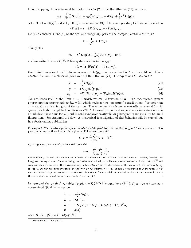
Upon dropping the o�-diagonal term of order � in (23), the Hamiltonian (22) becomesH0 = 12pTxH(y)px + 12pTyK(y)py +W (y) + 12xTH(y)xwith H(y) =D(y)2 and K(y);W (y) as de�ned in (21). The corresponding Lie-Poisson bracket isfF;Gg = ��1fF;Ggx;px + fF;Ggy;py :Next we consider x and px as the real and imaginary part of the complex vector z 2 Cm, i.e.z = 1p2 (x+ ipx) :This yields H0 = �zTH(y)z + 12pTyK(y)py +W (y)and we write this as a QCMD-like system with total energyH0 = hz;H(y)zi+Hc(y;py);the �nite dimensional \Schr�odinger operator" H(y), the \wave function" z, the arti�cial \Plankconstant" �, and the classical (constrained) Hamiltonian (21). The equations of motion are_z = � i�H(y)z; (24)_y = +rpyHc(y;py); (25)_py = �ryHc(y;py)�ryhz;H(y)zi: (26)We are interested in the limit � ! 0 which we will discuss in x4.3. The constrained systemapproximation corresponds to H0 = Hc which neglects the \quantum" contributions. We note thatI := hz; zi is a �rst integral of the system. The same quantity is not necessarily conserved for thesystem with the complete Hamiltonian (20).6 However, numerical experiments indicate that I isan adiabatic invariant for H� and is conserved over relatively long integration intervals up to small uctuations. See Example 3 below. A theoretical investigation of this behavior will be carried outin a forthcoming publication.Example 3. We consider a planar system consisting of six particles with coordinates qi 2 R2 and mass m = 1. Theparticles interact with each other through a (sti�) harmonic potentialVsti� = K2 5Xj=0(rj;j+1 � 1)2;rij = jjqi � qj jj, and a (soft) anharmonic potentialVsoft = 4Xj=0 6Xi=j+2 1rij :For simplicity, the �rst particle is �xed at zero. The force constant K is set to K = 2:5e+04; 1:0e+06; 1:0e+08. Weintegrate the equations of motion using the Verlet method with a su�ciently small step-size of �t = 0:1=pK andcompute the eigenvalues of the corresponding matrix H(y) 2 R5�5, the entries of the vector z 2 C5, and I = hz;zi.In Fig. 1, we plot the time evolution of I(t) over a time interval T = 120. It can be concluded that the norm of thevector z is relatively well conserved for our two time-scales CMD model. Numerical results on the time evolution ofthe individual entries of the vector z can be found in x4.3. �In terms of the original variables (q;p), the QCMD-like equations (24)-(26) can be written as aconstrained QCMD-like system_z = � i�H(q)z;_q = M�1p;_p = �rqV(q)�rqhz;H(q)zi �G(q)T�;0 = g(q)with H(q) = [G(q)M�1G(q)T ]1=2.6We have H� = H0 +O(�). 9

0 20 40 60 80 100 1201.2

1.3

1.4

1.5

1.6

K=2.5e+04

0 20 40 60 80 100 1201.2

1.3

1.4

1.5

1.6

K=1.0e+06

0 20 40 60 80 100 1201.2

1.3

1.4

1.5

1.6

K=1.0e+08Figure 1: Time evolution of I(t) over a time interval [0; 120] for di�erent values of the force constantK.4.3 The Limiting Behavior of the CMD ModelThe results of the previous section indicate that one can reduce the discussion of the limiting behaviorof the CMD model as � = K�1=2 ! 0 to the investigation of the QCMD-like equations (24)-(26).In case that H(y) is a scalar, i.e. H(y) = h(y) 2 R, no resonances can occur and the "Born-Oppenheimer" approximation is valid for all y. The averaged equations are_y = +rpyHc(y;py);_py = �ryHc(y;py)� jzj2ryh(y);jzj2 = const.The need for the correcting force term Fc = jzj2ryh(y) was �rst pointed out by Rubin & Ungar[36]. It was shown in [34] that the corresponding CMD equations satisfy jz(t)j � const. over anexponentially long time interval T � ec=�, c > 0 some constant, if the energy function (16) is realanalytic.Under the assumption that the fast degree of motion is strongly coupled to a heat bath withtemperature T , the correcting force term is determined by the relation jzj2h(y) = kBT and leads tothe Fixman potential Vc = kBT lnh(y) [18, 32].If a given matrix valued H(y) can be smoothly diagonalized, then we can still apply the \Born-Oppenheimer" approximation provided the eigenvalues of the matrix H(y) are all di�erent. Thiscase was �rst investigated by Takens in [41]. For a recent discussion in terms of homogenizationsee [11]. If eigenvalues cross, then the \Born-Oppenheimer" approximation breaks down as for theQCMD model of x3. See the numerical example below.The correcting force term vanishes ifH(y) =H = const. This situation occurs if the constrainedHamiltonian (21) corresponds to a system of uncoupled rigid bodies, i.e. G(q)M�1G(q)T = const.,10

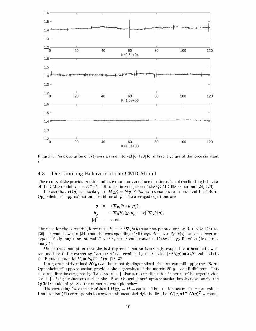
and has been analysed by Benettin, Galgani & Giorgilli in [5].Example 3. (cont.) In Fig. 2, we present the eigenvalues of the \Schr�odinger" matrix H(y) and the \occupationnumbers" jzi(t)j2, i = 1; : : : ; 5, corresponding to the \wave" vector z(t). The force constant was set equal toK = 2:5e+04. \Occupation numbers" jzi(t)j2 jump when the corresponding eigenvalues undergo or are close to a1 : 1 resonance (except at t � 22:2). It should be noted that higher-order resonances do not lead to transitions in the\occupation numbers". This is contrary to what can be expected from the results presented in [41, 11]. �

20 21 22 23 24 25 26 27 28 29 300

0.5

1

1.5

2

eige

nval

ues

20 21 22 23 24 25 26 27 28 29 300

0.1

0.2

0.3

0.4

0.5

0.6

0.7

K=2.5e+04

occu

patio

n nu

mbe

rs

Figure 2: Time evolution of the eigenvalues of H(y) and the corresponding \occupation numbers"jzi(t)j2, i = 1; : : : ; 5, for K = 2:5e+04 and over the time interval [20; 30].5 Multiple Time Stepping for Classical MDThe analysis of x4 indicates that in most cases the fast oscillations cannot be eliminated (or ig-nored) in long term MD simulations. In particular, non-adiabatic transitions and the break-down ofthe \Born-Oppenheimer" approximation are unavoidable. The best way out might be an e�cientsimulation of the full system which takes into account the existing multiple time scales. Since thestandard MTS method (5) su�ers from resonance induced instabilities [7], we will discuss a variantof the molli�ed MTS methods, as suggested in [19], that is particularly suited for the CMD model.5.1 Projected Multiple-Time-SteppingLet us come back to highly oscillatory Hamiltonian systems of type_q = M�1p;_p = �rqV(q)�G(q)TKg(q) :11

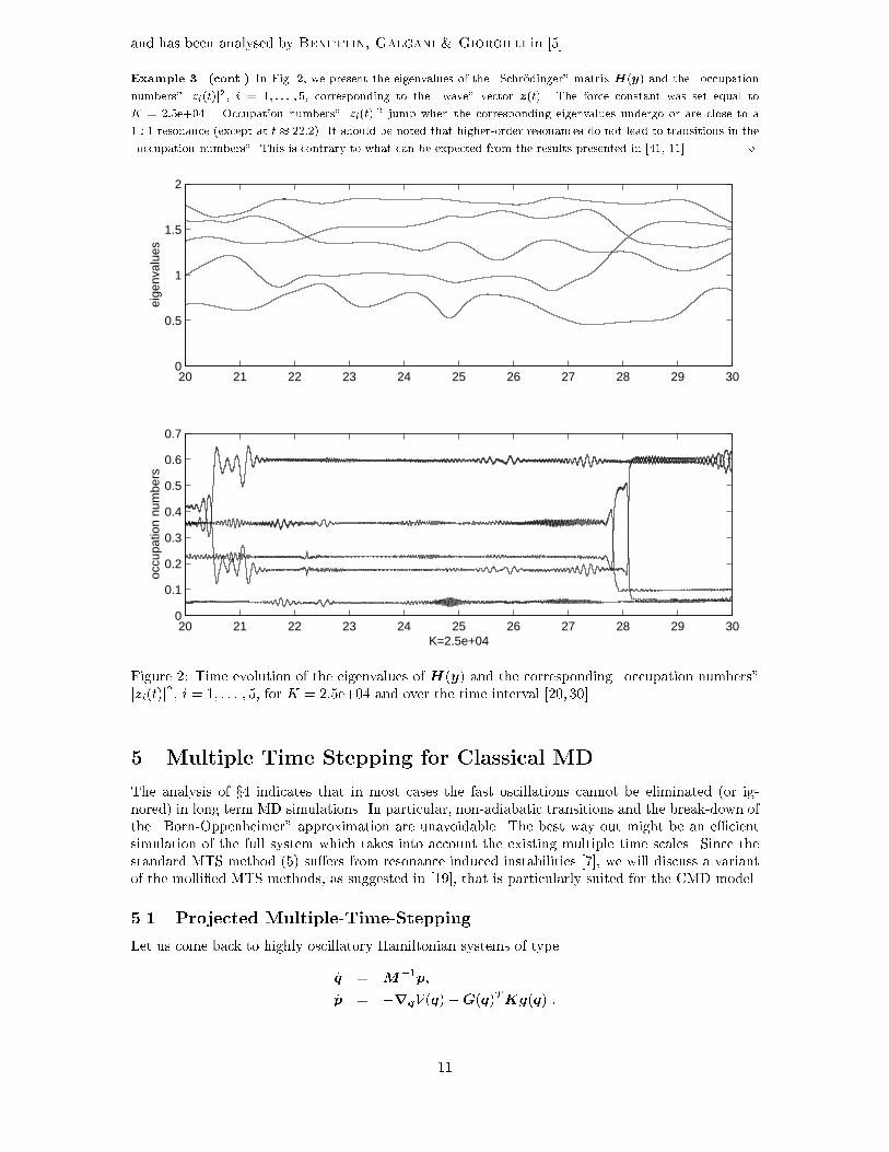
Step 1.�pn = pn � �t2 rqU2(qn)Step 2.Integrate the fast/local systemddtq = M�1p;ddtp = �rqU1(q)using Verlet with a step-size �t = �t=j, j � 1, and initial conditions(qn; �pn). Denote the result by (qn+1; �pn+1).Step 3.pn+1 = �pn+1 � �t2 rqU2(qn+1)Figure 3: Standard Multiple-Time-SteppingThe Hamiltonian is H(q;p) = pTM�1p2 + V(q) + g(q)TKg(q)2and we split the potential energy V into a short range contribution V1 and a long range contributionV2. The standard MTS method [7, 23, 42] is now de�ned via the splittingH = T (p) + U1(q) + U2(q)with U2 = V2 and U1 = V1 + 1=2g(q)TKg(q). This leads to the MTS algorithm (5) which is moreexplicitly written out in Fig. 3.This formulation su�ers from resonance induced instabilities [7, 9] which is caused by an un-fortunate sampling of the high-frequency oscillations in q1 = g(q). In [19], Garc�ia-Archilla,Sanz-Serna & Skeel suggested to combine averaging with multiple-time-stepping. Here we useinformation about the analytical solution behavior of the fast system to obtain the averaged force�eld.The motion in q1 := g(q) is highly oscillatory with a time-average close to zero. To eliminatethe e�ect of the highly oscillatory variable q1 on the long range forces in (5), we replace the longrange force �eld F 2(q) = �rqU2(q) by�F 2(q) = �rqU2( (q))which is the gradient of the modi�ed potential energy W (q) := U2( (q)).The function is de�ned by the SHAKE-like nonlinear system of equations~q = (q) = q +M�1G(q)T � ;0 = g(~q)in the variable � 2 Rm. Note that projects the q1 = g(q) solution component to zero. Toimplement our approach, we need the Jacobian @q of . This requires the computation of thesecond derivative @qqgi(q) of the functions gi, i = 1; : : : ;m, and the solution of a linear system ofequations, i.e., d~q = dq +M�1G(q)T d�+M�1 mXi=1 �i @qqgi(q)dq;0 = G(~q)d~q 12

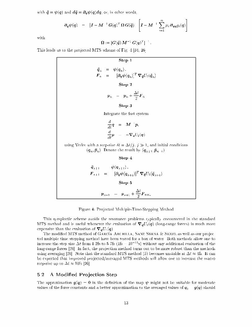
with ~q = (q) and d~q = @q (q)dq, or, in other words,@q (q) = �I �M�1G(q)T G(~q)� "I +M�1 mXi=1 �i @qqgi(q)#with := [G(~q)M�1G(q)T ]�1 :This leads us to the projected MTS scheme of Fig. 4 [34, 26].Step 1.~qn = (qn) ;F n = �[@q (qn)]T r~qU2(~qn)Step 2.�pn = pn + �t2 F nStep 3.Integrate the fast systemddtq = M�1p;ddtp = �rqU1(q)using Verlet with a step-size �t = �t=j, j � 1, and initial conditions(qn; �pn). Denote the result by (qn+1; �pn+1).Step 4.~qn+1 = (qn+1) ;F n+1 = �[@q (qn+1)]T r~qU2(~qn+1)Step 5.pn+1 = �pn+1 + �t2 F n+1Figure 4: Projected Multiple-Time-Stepping MethodThis symplectic scheme avoids the resonance problems typically encountered in the standardMTS method and is useful whenever the evaluation of rqU2(q) (long-range forces) is much moreexpensive than the evaluation of rqU1(q).The modi�ed MTS method of Garc�ia-Archilla, Sanz-Serna & Skeel as well as our projec-ted multiple-time-stepping method have been tested for a box of water. Both methods allow one toincrease the step-size �t from 1-2fs to 5-7fs (1fs = 10�15s) without any additional evaluation of thelong-range forces [26]. In fact, the projection method turns out to be more robust than the methodsusing averaging [26]. Note that the standard MTS method (5) becomes unstable at �t � 4fs. It canbe expected that improved projected/averaged MTS methods will allow one to increase the macrostep-size up to �t � 10fs [26].5.2 A Modi�ed Projection StepThe approximation g(q) = 0 in the de�nition of the map might not be suitable for moderatevalues of the force constants and a better approximation to the averaged values of q1 = g(q) should13

be used. As pointed out in [33, 44], the variable q1 oscillates about the minimum of the total energyin the direction of q1. This minimum is characterized7 by the nonlinear equation0 = G(~q)M�1r~qU1(~q)which replaces the constraint g(q) = 0. Thus we introduce the modi�ed projection~q := �(q)by means of ~q := q +M�1G(q)T � ;0 = G(~q)M�1r~qU1(~q): (27)The resulting nonlinear system in the variable � 2 Rm can be solved by Newton's method with thesimpli�ed (symmetric) JacobianJ = [G(q)M�1G(q)T ]K [G(q)M�1G(q)] :As before, we introduce a modi�ed (averaged) long range potential energy functionW (q) := U2(�(q)):The evaluation of the gradient rqW (q) = [@q�(q)]Tr~qU2(~q)requires the computation of @q�(q), i.e.d~q := @q�(q)dq ;= dq +M�1G(q)T d� +M�1 mXi=1 �i @qqgi(q)dq;and d� is determined by the equation0 = @~q �G(~q)M�1r~q U1(~q)� d~q:In terms of the individual functions gi, this results in0 = n�M�1r~q U1(~q)�T @~q~qgi(~q) +Gi(~q)M�1@~q~qU1(~q)od~qwhich includes the computation of the Hessian of U1(q). Thus this approach should only be used ifU1 is restricted to nearest neighborhood interactions such as the bond stretching/bending potentialsand the repulsive part of the Lennard-Jones interactions.The modi�ed projection can be built into the MTS scheme of Fig. 4 by replacing by �. Welike to point out that this modi�ed force �eld requires additional force �eld evaluations. However,these additional force �eld evaluations are restricted to nearest neighborhood interactions.6 Multiple Time Stepping for Quantum-Classical MDA natural extension [30] of the Verlet method to the QCMD equations of motion is given by n+1=2 = exp ��i�t2~H(qn)� n; (28)Leapfrog8>>>>><>>>>>: qn+1=2 = qn + �t2 M�1pn;pn+1 = pn ��t h n+1=2;rqH(qn+1=2) n+1=2i ��trqU(qn+1=2);qn+1 = qn+1=2 + �t2 M�1pn+1; (29) n+1 = exp ��i�t2~H(qn+1)� n+1=2: (30)7Here we have neglected velocity dependent contributions and contributions from the long range potential energyU2(q). 14

Even if the matrix exponentials in (28) and (30) are evaluated exactly, the scheme requires a verysmall step-size. Otherwise the Hellmann-Feynman forces acting on the classical coordinates willbe wrongly approximated [24, 30, 31] and the behavior of the populations fj�i(t)j2g may not bereproduced correctly (see Example 4 below). The same holds true for MTS variants of the abovemethod, as suggested in [38, 39], where the matrix exponential is replaced by an approximationusing j steps of a smaller step-size �t = �t=j.Example 4. We like to demonstrate a potentially dangerous implication of using a large time-step on the preservationof the populations fj�i(t)j2g in an adiabatic regime. Let us consider a simple two dimensional system_ = � i~H(t) ; (31) 2 C2, where the dependence of H on the classical coordinate q is replaced by a time dependence. In particular, wetake H(t) = � cos2 t � sin2 t �2 cos t sin t�2 cos t sin t sin2 t� cos2 t �and introduce a new vector � by � = Q(t) with Q(t) = � cos t � sin tsin t cos t � :This transformation gives rise to the equation _� = � i~E� +A�with E := � 1 00 �1 �and A := � 0 �11 0 � :Provided ~ � 1, this system satis�es the quantum adiabatic theorem which implies that the populations fj�i(t)j2gare almost constant.An exponential integrator for the system (31) is given by n+1 = exp�� i�t2~ Hn+1� exp�� i�t2~ Hn� n= QTn+1 exp�� i�t2~ E�Qn+1QTn exp�� i�t2~ E�Qn nor, in terms of �, as �n+1 = exp�� i�t2~ E�Qn+1QTn exp�� i�t2~ E� �n: (32)Let us assume that the step-size �t is (accidentally) chosen such thatexp�� i�t2~ E� = I;then (32) \simpli�es" to �n+1 = Qn+1QTn�nwhich is a second order accurate discretization of the di�erential equation_� = A� = _Q(t)Q(t)T �:But this is wrong. The populations fj�i(t)2jg are no longer conserved but undergo a systematic drift instead.We like to point out that this e�ect is due to a unfortunate choice of the step-size �t and may not beobserved generally. Nevertheless, it raises concerns about using a large time-step when integrating a slowly varyingtime-dependent Schr�odinger equation. �Provided that we can neglect the problem mentioned in Example 4, a larger macro step-size �t maybe applied in (28)-(30), if the Born-Oppenheimer approximation (14) to the Hellmann-Feynmanforce is used in (29). See [8] for details. However, the formula (14) requires the computation of thederivatives of the diagonalized quantum operatorE(q) which is computational expensive, in general.15

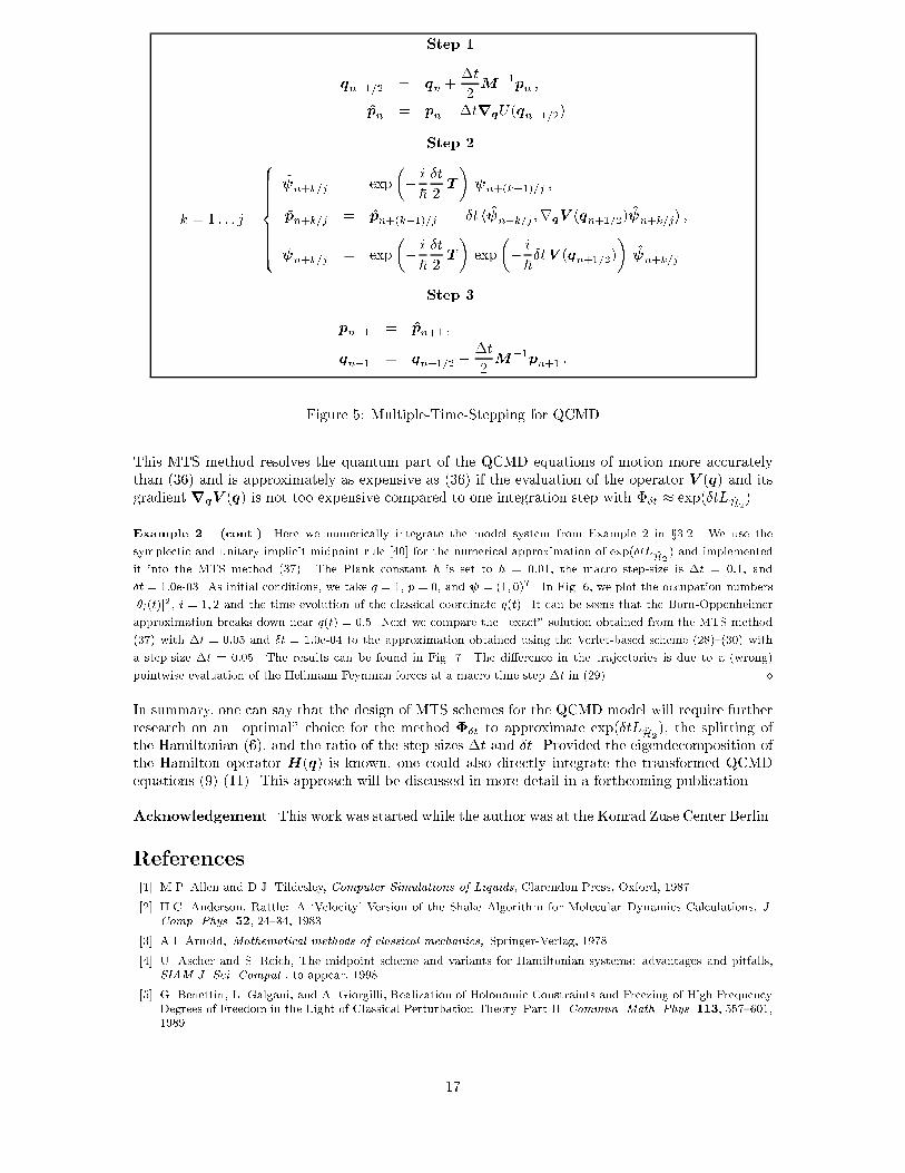
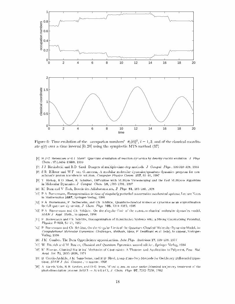
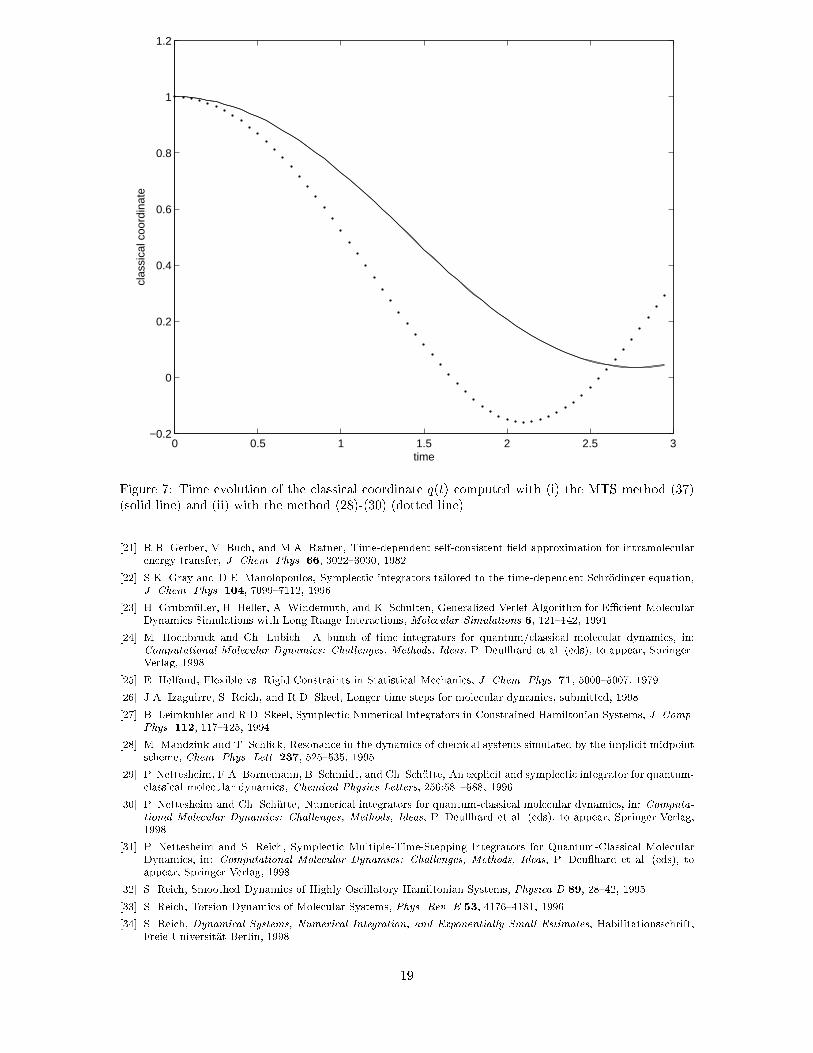
This can be avoided if an explicit averaging along (t) is applied to the Hellmann-Feynman forcein (29). See [24] for details.Here we suggest a di�erent approach based on a splitting of the Hamiltonian (6) intoH = H1+H2in the following way [31]:H1 = pTM�1p2 and H2 = h ;H(q) i+ U(q) :Let us write down the corresponding di�erential equations. First for H1:_ = 0 ;_q = M�1p ;_p = 0 ;next for H2: _ = � i~H(q) ; (33)_q = 0 ; (34)_p = �h ;rqH(q) i �rqU(q) : (35)The solution to H1 is just a translation of classical particles with constant momentum p.The intriguing point about the second set of equations is that q is now kept constant. Thus thevector evolves according to a time-independent Schr�odinger equation with constant HamiltonianoperatorH(q) and the update of the classical momentum p is obtained by integrating the Hellmann-Feynman forces [12] acting on the classical particles along the computed (t) (plus a constant updatedue to the purely classical force �eld).Upon computing the eigenvalues of the operator H(q), the equations (33)-(35) can be solvedexactly. However, this is, in general, an expensive undertaking. Therefore we proceed with thefollowing multiple-time-stepping approach: The �rst step is to consider the identityexp(�tLH2) = exp(�tLH2) � exp(�tLU ) = exp(�tLH2)| {z }j times � exp(�tLU ) ;where �t = �t=j, j � 1, and H2 = h ;H(q) i :The second step is to useexp(�tLH) = exp(�t2 LH1) � exp(�tLH2)| {z }j times � exp(�tLU ) � exp(�t2 LH1) +O(�t3) : (36)The last step is to �nd a symplectic, second order approximation ��t to exp(�tLH2). In principle,we can use any symplectic integrator suitable for time-dependent Schr�odinger equations with atime-independent Hamilton operator H(q) (see, for example, [22]).Provided that V (q) is diagonal, an e�cient method ��t is obtained by exploiting the naturalsplitting of the quantum operatorH(q) = T +V (q) as used in the symplectic PICKABACK scheme[29]. This yields two exactly solvable subsystemsH2;1 = h ;T i and H2;2 = h ;V (q) i :The resulting integrator for QCMD, as presented in Fig. 5 and �rst suggested in [31], is of secondorder, explicit, symplectic, and conserves the norm of the wave-function. For the implementation ofother choices for ��t, see [31].The MTS scheme of Fig. 5 may still require a relatively small macro step-size �t to insure anaccurate computation of the populations fj�i(t)j2g. Thus it might be useful to consider the followingmodi�cation of the MTS scheme (36):exp(�t2 LU ) � 2664exp(�t2 LH1) � exp(�tLH2) � exp(�t2 LH1)| {z }j times 3775 � exp(�t2 LU ) : (37)16

Step 1.qn+1=2 = qn + �t2 M�1pn ;pn = pn ��trqU(qn+1=2)Step 2.k = 1 : : : j 8>>>>>><>>>>>>: n+k=j = exp�� i~ �t2 T� n+(k�1)=j ;pn+k=j = pn+(k�1)=j � �t h n+k=j ;rqV (qn+1=2) n+k=ji ; n+k=j = exp�� i~ �t2 T� exp�� i~�tV (qn+1=2)� n+k=jStep 3.pn+1 = pn+1 ;qn+1 = qn+1=2 + �t2 M�1pn+1 :Figure 5: Multiple-Time-Stepping for QCMDThis MTS method resolves the quantum part of the QCMD equations of motion more accuratelythan (36) and is approximately as expensive as (36) if the evaluation of the operator V (q) and itsgradient rqV (q) is not too expensive compared to one integration step with ��t � exp(�tLH2).Example 2. (cont.) Here we numerically integrate the model system from Example 2 in x3.2. We use thesymplectic and unitary implicit midpoint rule [40] for the numerical approximation of exp(�tLH2 ) and implementedit into the MTS method (37). The Plank constant ~ is set to ~ = 0:01, the macro step-size is �t = 0:1, and�t = 1:0e-03. As initial conditions, we take q = 1, p = 0, and = (1; 0)T . In Fig. 6, we plot the occupation numbersj�i(t)j2, i = 1; 2 and the time evolution of the classical coordinate q(t). It can be seens that the Born-Oppenheimerapproximation breaks down near q(t) = 0:5. Next we compare the \exact" solution obtained from the MTS method(37) with �t = 0:05 and �t = 1:0e-04 to the approximation obtained using the Verlet-based scheme (28){(30) witha step-size �t = 0:05. The results can be found in Fig. 7. The di�erence in the trajectories is due to a (wrong)pointwise evaluation of the Hellmann-Feynman forces at a macro time step �t in (29). �In summary, one can say that the design of MTS schemes for the QCMD model will require furtherresearch on an \optimal" choice for the method ��t to approximate exp(�tL ~H2), the splitting ofthe Hamiltonian (6), and the ratio of the step-sizes �t and �t. Provided the eigendecomposition ofthe Hamilton operator H(q) is known, one could also directly integrate the transformed QCMDequations (9)-(11). This approach will be discussed in more detail in a forthcoming publication.Acknowledgement. This work was started while the author was at the Konrad Zuse Center Berlin.References[1] M.P. Allen and D.J. Tildesley, Computer Simulations of Liquids, Clarendon Press, Oxford, 1987.[2] H.C. Anderson, Rattle: A `Velocity' Version of the Shake Algorithm for Molecular Dynamics Calculations, J.Comp. Phys. 52, 24{34, 1983.[3] A.I. Arnold, Mathematical methods of classical mechanics, Springer-Verlag, 1978.[4] U. Ascher and S. Reich, The midpoint scheme and variants for Hamiltonian systems: advantages and pitfalls,SIAM J. Sci. Comput., to appear, 1998.[5] G. Benettin, L. Galgani, and A. Giorgilli, Realization of Holonomic Constraints and Freezing of High FrequencyDegrees of Freedom in the Light of Classical Perturbation Theory. Part II. Commun. Math. Phys. 113, 557{601,1989. 17

0 2 4 6 8 10 12 14 16 18 200

0.2

0.4

0.6

0.8

1

occu

patio

n nu

mbe

rs

0 2 4 6 8 10 12 14 16 18 200

0.5

1

1.5

2

clas

sica

l coo

rdin

ate

timeFigure 6: Time evolution of the \occupation numbers" j�i(t)j2, i = 1; 2, and of the classical coordin-ate q(t) over a time interval [0; 20] using the symplectic MTS method (37).[6] H.J.C. Berendsen and J. Mavri. Quantum simulation of reaction dynamics by density matrix evolution. J. Phys.Chem., 97:13464{13468, 1993.[7] J.J. Biesiadecki and R.D. Skeel. Dangers of multiple-time-step methods. J. Comput. Phys., 109:318{328, 1993.[8] S.R. Billeter and W.F. van Gunsteren, A modular molecular dynamics/quantum dynamics program for non-adiabatic proton transfers in solution, Computer Physics Comm. 107, 61{91, 1997.[9] T. Bishop, R.D. Skeel, K. Schulten, Di�culties with Multiple Timestepping and the Fast Multipole Algorithmin Molecular Dynamics, J. Comput. Chem. 18, 1785{1791, 1997.[10] M. Born and V. Fock, Beweis des Adiabatensatzes, Z. Phys. 51, 165{180, 1928.[11] F.A. Bornemann, Homogenization in time of singularly perturbed conservative mechanical systems, Lecture Notesin Mathematics 1687, Springer-Verlag, 1998.[12] F.A. Bornemann, P. Nettesheim, and Ch. Sch�utte, Quantum-classical molecular dynamics as an approximationfor full quantum dynamics, J. Chem. Phys. 105, 1074{1083, 1996.[13] F.A. Bornemann and Ch. Sch�utte, On the singular limit of the quantum-classical molecular dynamics model,SIAM J. Appl. Math., to appear, 1998.[14] F. Bornemann and Ch. Sch�utte, Homogenization of Hamiltonian Systems with a Strong Constraining Potential,Physica D 102, 57{77, 1997.[15] F. Bornemann and Ch. Sch�utte, On the Singular Limit of the Quantum-Classical Molecular Dynamics Model, in:Computational Molecular Dynamics: Challenges, Methods, Ideas, P. Deu hard et al. (eds), to appear, Springer-Verlag, 1998.[16] J.M. Combes, The Born-Oppenheimer approximation, Acta Phys. Austriaca 17, 139{159, 1977.[17] W. Dittrich and M. Reuter, Classical and Quantum Dynamics, second edition, Springer-Verlag, 1994.[18] M. Fixman, Classical Statistical Mechanics of Constraints: A Theorem and Application to Polymers, Proc. Nat.Acad. Sci. 71, 2635{2638, 1974.[19] B. Garc��a-Archilla, J.M. Sanz-Serna, and R.D. Skeel, Long-Time-Step Methods for Oscillatory Di�erential Equa-tions, SIAM J. Sci. Comput., to appear, 1998.[20] A. Garc��a-Vela, R.B. Gerber, and D.G. Imre, Mixed quantum wave packet/classical trajectory treatment of thephotodissociation process ArHCl ! Ar+H+Cl, J. Chem. Phys. 97, 7242{7250, 1992.18

0 0.5 1 1.5 2 2.5 3−0.2

0

0.2

0.4

0.6

0.8

1

1.2

time

clas

sica

l coo

rdin

ate

Figure 7: Time evolution of the classical coordinate q(t) computed with (i) the MTS method (37)(solid line) and (ii) with the method (28)-(30) (dotted line).[21] R.B. Gerber, V. Buch, and M.A. Ratner, Time-dependent self-consistent �eld approximation for intramolecularenergy transfer, J. Chem. Phys. 66, 3022{3030, 1982.[22] S.K. Gray and D.E. Manolopoulos, Symplectic integrators tailored to the time-dependent Schr�odinger equation,J. Chem. Phys. 104, 7099{7112, 1996.[23] H. Grubm�uller, H. Heller, A. Windemuth, and K. Schulten, Generalized Verlet Algorithm for E�cient MolecularDynamics Simulations with Long-Range Interactions, Molecular Simulations 6, 121{142, 1991.[24] M. Hochbruck and Ch. Lubich. A bunch of time integrators for quantum/classical molecular dynamics, in:Computational Molecular Dynamics: Challenges, Methods, Ideas, P. Deu hard et al. (eds), to appear, Springer-Verlag, 1998.[25] E. Helfand, Flexible vs. Rigid Constraints in Statistical Mechanics, J. Chem. Phys. 71, 5000{5007, 1979.[26] J.A. Izaguirre, S. Reich, and R.D. Skeel, Longer time steps for molecular dynamics, submitted, 1998.[27] B. Leimkuhler and R.D. Skeel, Symplectic Numerical Integrators in Constrained Hamiltonian Systems, J. Comp.Phys. 112, 117{125, 1994.[28] M. Mandziuk and T. Schlick, Resonance in the dynamics of chemical systems simulated by the implicit midpointscheme, Chem. Phys. Lett. 237, 525{535, 1995.[29] P. Nettesheim, F.A. Bornemann, B. Schmidt, and Ch. Sch�utte, An explicit and symplectic integrator for quantum-classical molecular dynamics, Chemical Physics Letters, 256:581{588, 1996.[30] P. Nettesheim and Ch. Sch�utte, Numerical integrators for quantum-classical molecular dynamics, in: Computa-tional Molecular Dynamics: Challenges, Methods, Ideas, P. Deu hard et al. (eds), to appear, Springer-Verlag,1998.[31] P. Nettesheim and S. Reich, Symplectic Multiple-Time-Stepping Integrators for Quantum-Classical MolecularDynamics, in: Computational Molecular Dynamics: Challenges, Methods, Ideas, P. Deu hard et al. (eds), toappear, Springer-Verlag, 1998.[32] S. Reich, Smoothed Dynamics of Highly Oscillatory Hamiltonian Systems, Physica D 89, 28{42, 1995.[33] S. Reich, Torsion Dynamics of Molecular Systems, Phys. Rev. E 53, 4176{4181, 1996.[34] S. Reich, Dynamical Systems, Numerical Integration, and Exponentially Small Estimates, Habilitationsschrift,Freie Universit�at Berlin, 1998. 19

[35] S. Reich, A modi�ed force �eld for constrained molecular dynamics, Numerical Algorithms, to appear, 1998.[36] H. Rubin and P. Ungar, Motion Under a Strong Constraining Force, Comm. Pure Appl. Math. 10, 65{87, 1957.[37] J.P. Ryckaert, G. Ciccotti, H.J.C. Berendsen, Numerical Integration of the Cartesian Equations of Motion of aSystem with Constraints: Molecular Dynamics of n-Alkanes, J. Comput. Phys. 23, 327{342, 1977.[38] U. Schmitt and J. Brinkmann, Discrete time-reversible propagation scheme for mixed quantum classical dynamics,Chem. Phys., 208, 45{56, 1996.[39] U. Schmitt, Gemischt klassisch-quantenmechanische Molekulardynamik im Liouville-Formalismus, Ph.D. thesis(in german), Darmstadt, 1997.[40] J.M. Sanz-Serna and M.P. Calvo, Numerical Hamiltonian Systems, Chapman and Hall, London, 1994.[41] F. Takens, Motion Under the In uence of a Strong Constraining Force, in: Global Theory of Dynamical Systems,Lecture Notes Math. 819, 425{445, 1980.[42] M. Tuckerman, B.J. Berne, and G.J. Martyna, Reversible Multiple Time Scale Molecular Dynamics, J. Chem.Phys. 97, 1990{2001, 1992.[43] L. Verlet, Computer Experiments on Classical Fluids. I. Thermodynamical Properties of Lennard-Jones Mo-lecules, Phys. Rev. 159, 1029{1039, 1967.[44] J. Zhou, S. Reich, and B.R. Brooks, Elastic Molecular Dynamics with Flexible Constraints, submitted, 1998.

20