multiple sourcing effects in the expansion of panama canal
TRANSCRIPT
The Pennsylvania State University
The Graduate School
College of Engineering
MULTIPLE SOURCING EFFECTS IN THE EXPANSION OF PANAMA CANAL
A Thesis in
Industrial Engineering and Operations Research
by
Yuexi Chen
©2014 Yuexi Chen
Submitted in Partial Fulfillment
of the Requirements
for the Degree of
Master of Science
August 2014

ii
The thesis of Yuexi Chen was reviewed and approved* by the following:
Vittal Prabhu
Professor, Department of Industrial and Manufacturing Engineering
Thesis Adviser
Saurabh Bansal
Assistant Professor, Department of Supply Chain and Information Systems
Paul Griffin
Professor, Department of Industrial and Manufacturing Engineering
Peter and Angela Dal Pezzo Department Head Chair
*Signatures are on file in the Graduate School.

iii
ABSTRACT
With the expanding of Panama Canal, suppliers along the East coast are facing challenges
of shift in cargo, while customers earn benefits for more suppliers to choose from. The
study will discuss the impact of Panama Canal expansion along the supply chain, by
analyzing the change of risk and uncertainty due to involvement of multiple suppliers
(sources); and give customers insights of how to choose among a number of suppliers.
The Panama Canal expansion problem will be fitted into a Beer Game model with
multiple suppliers. Later in the article will analyze the problem by using various kinds of
optimization methods in the area of supply chain management. Detailed problem
formulation will be provided with multiple criteria. After that recommendations will be
made to the customers.

iv
Table of Contents
List of Figures .................................................................................................................... v
List of Tables .................................................................................................................... vi
Chapter 1. Literature Review ............................................................................................ 1
Chapter 2. Research Methodology .................................................................................. 11
Chapter 3. An EOQ Model Evaluating Purchase from Multiple Suppliers to Single
Destination ........................................................................................................................ 13
Problem Statement and Assumptions ............................................................................ 13
Evaluation of Order Fulfillment Rate............................................................................ 14
Optimization Model Formulation ................................................................................. 18
Numerical Example ....................................................................................................... 21
Chapter 4. Optimization of Performance Measures ........................................................ 24
Excel Solver VBA ......................................................................................................... 24
Interior-Point Method .................................................................................................... 26
Augmented Simultaneous Perturbation Stochastic Approximation (ASPSA) method . 28
A Comparison between VBA and Matlab..................................................................... 32
A Comparison between Interior Point Method and ASPSA Method............................ 32
Chapter 5. A Multiple Criteria Model to Evaluate Performance Measures .................... 37
Goal Programming ........................................................................................................ 37
Goal Programming Model ............................................................................................. 38
Chapter 6. Conclusion ..................................................................................................... 41
Appendix A ...................................................................................................................... 43
VBA Code ..................................................................................................................... 43
Interior-Point Method .................................................................................................... 44
ASPSA Method ............................................................................................................. 47
Goal Programming ........................................................................................................ 53
Biography......................................................................................................................... 57
v
List of Figures
Figure 1.Waterway Routes between Far East and the US .................................................. 2
Figure 2. Beer Game ........................................................................................................... 3
Figure 3. Variability of Orders............................................................................................ 4
Figure 4. Variability of Inventory ....................................................................................... 4
Figure 5. Demand Distortion .............................................................................................. 5
Figure 6. Dependency Analysis .......................................................................................... 6
Figure 7. The change of 50 variables for 150000 iterations for maximizing A ................ 30
Figure 8. The change of objective A for 150000 iterations .............................................. 31
Figure 9. The change of 50 variables for 150000 iterations for minimizing B ................ 31
Figure 10. The change of objective B for 150000 iterations ............................................ 32
Figure 11. Comparison between Interior Point and ASPSA on Obj A ............................. 34
Figure 12. Comparison between Interior Point and ASPSA on Time to compute A ....... 34
Figure 13. Comparison between Interior Point and ASPSA on Obj B ............................. 35
Figure 14. Comparison between Interior Point and ASPSA on Time to compute B........ 35

vi
List of Tables
Table 1. Numerical Example Parameters .......................................................................... 22
Table 2. A Feasible Solution ............................................................................................. 23
Table 3. VBA Result for Optimizing A ............................................................................ 25
Table 4. VBA Result for Optimizing B ............................................................................ 25
Table 5. Interior-Point Method for Optimizing A ............................................................ 27
Table 6. Interior-Point Method for Optimizing B ............................................................. 27
Table 7. ASPSA Method for Optimizing A ...................................................................... 30
Table 8. ASPSA Method for Optimizing B ...................................................................... 30
Table 9. Results Comparison between Interior-Point and ASPSA ................................... 33
Table 10. Further Comparison between Interior-Point and ASPSA ................................. 33
Table 11. Goal Programming Results ............................................................................... 40

vii
Acknowledgements
This thesis has been successfully completed under hard work, supports and continuous
efforts from many individuals, supervisors and institutions.
First and foremost, I would like to specially thank to Dr. Vittal Prabhu, my thesis advisor,
for his valuable guidance and instructions. It always brings me inspiration when
discussing with him.
Besides, I would like to thank to the Department of Industrial and Manufacturing
Engineering of the Pennsylvania State University for providing me rich resources and
good facilities to complete this thesis.
Last but not least, I deeply appreciate the understanding and supports from my family and
friends on me in completing the thesis.

1
Chapter 1
Literature Review
Panama Canal Expansion
A large part of Sino-US trade is conducted through entrepot trade on the US West coast.
Container vessels larger than 5,000 TEU transport goods from China to the US West
coast, then dispatch goods to the East coast via land way. The tedious processes lead to
port congestion, additional cost of switching transportation means and thus, low
efficiency.
The Panama Canal’s massive expansion project has been started in 2007, and is
scheduled to be completed in 2015. By the time, the Canal will allow large container
vessels with up to 13,000 TEU shipping capacity to transport through waterway directly
from Far East to the US East coast. The project will steal the show of the West coast
harbors and spurs East coast harbors to undertake multimillion-dollar efforts to increase
their capacity and local infrastructure.
By the time of completion of the project, new patterns of logistics planning will reveal on
the East coast due to larger goods supply directly shipped to there, and more retailers
involved in. In a typical supply chain, if we call the East coast harbors as the “suppliers”,
then inland supermarkets that needs goods supplies from harbors can be considered as
“customers”. From a customer’s point of view, the situation of more suppliers gives
chance to lower cost and improve efficiency. At this point, interesting questions are
raised: how to make the best selection among retailers? What are the criteria when

2
making selection? We can model the situation as a multiple sourcing problem and
analyze it by using supply chain management methods.
Figure 1.Waterway Routes between Far East and the US
(Source: Maritime Construction Depot [3])
The Beer Game
The Beer Game is a logistics simulation game that demonstrates basic principles in
supply chain management. First developed by a group of professors of MIT in 1960s, the
beer game has since been played all over the globe from all levels. The objective of the
game is to meet end customer’s demand of product while keeping as less penalty cost
(inventory cost and backorder cost) as possible along supply chain.
Typically, the beer game includes four stages: factory, distributor, wholesaler and retailer.
The factory produce product while the other three delivers product downward until it
reaches external end customer. They align as shown in flow chart in Figure 1. In this
system, retailer’s demands trigger product flow and order flow along the supply chain.

3
Before start, each stage has its own amount of inventory. The game is played in rounds,
which simulate weeks. For each round, each stage push an anticipated amount of product
downwards the supply chain, place an anticipated order upwards, and mark down
inventory level or backorder amount.
Figure 2. Beer Game
Some essential rules need to be followed. First, every order has to be fulfilled either
directly in current round, or later in subsequent rounds. Second, for penalty cost, each
item in inventory will cost $A per round, while each item in backorder will cost $B per
round. As mentioned above, the primary goal of the game is to minimize penalty cost.
Third, no communication is allowed among all stages. The only information allowed to
exchange is their orders. However, only the adjacent upstream stage can know the order.
Only the retailer knows the exact amount of order from external end customers while the
other three stages place anticipated orders base on their business intuition and
experiences.
Bullwhip Effect
The beer game would never failed to yield a bullwhip effect along the supply chain. If
consolidate and plot data collected from each stage, one can easily find that the
fluctuation of order amount and inventory level becomes more and more obvious on

4
upper stream stages. Two sample plots regarding the variability of order and inventory
are shown in Figure 3 and Figure 4. The data used in generating these two plots are from
a simulation of the game.
Figure 3. Variability of Orders
Figure 4. Variability of Inventory
0
10
20
30
40
50
60
70
80
0 5 10 15 20 25 30 35 40
Orders
Customer Retailer Wholesaler Distributor Factory
-150
-100
-50
0
50
0 5 10 15 20 25 30 35 40
Inventory
Retailer Wholesaler Distributor Factory

5
Bullwhip effect is the inherent increase in order amount fluctuation up the supply chain
(i.e., away from customer). As the illustration shown in Figure 5, the demand becomes
more and more distorted from downstream to upstream of the supply chain.
Figure 5. Demand Distortion
The concept of bullwhip effect first appeared in Forrester’s Industrial Dynamics in 1961.
Burbidge (1989) explained the behavior and called it the ‘Law of Industrial Dynamics’.
When demand of products is transmitted from downstream to upstream using stock
control ordering, then demand variation will be enlarged in each stage (Mason-Jones and
Towill 2000). According to Wilck (2006), the bullwhip effect is led from myopically
forecasted demand, order batching, price fluctuation and shortage gaming. It will result in
inventories excess, costs increase, quality problems, overtime expenses, shipping costs
increase, loss of customer service, lead time lengthening, sales loss and unnecessary
adjustment on capacity (Donovan 2002). Metters (1997) suggested that by reducing the
bullwhip effect the costs can be reduced dramatically. Even though the uncertainty is first
introduced by external end customers, the major amount uncertainty along the supply
chain is induced and magnified inside the system (Hieber and Hartel 2003). Information

6
sharing and coordination among stages within the supply chain are two well-known
management techniques, but it is often hard to do so.
Single Sourcing and Multiple Sourcing
According to Ford et al. (2011), single sourcing has the following benefits: single
agreement and one line of contact, and release from most of the day-to-day monitoring
and operation. But some risks such as higher supplier service responsibility, long-term
contract, and less competition, are more obvious. Multiple sourcing involves competition
between suppliers and avoid lock-in to a single supplier, tends to lead to shorter term
contract, and provides flexibility to replace a supplier without affecting others. However
more efforts shall be made by the customer to manage a portfolio of suppliers. To
evaluate supply chain risk associated with single vs. multiple sourcing, Nelson (2013)
conducted a mutual vs. lopsided dependency analysis. Customer with single sourcing is
more dependent than the supplier. If an issue arises, a transition to a multiple sourcing
strategy would help to mitigate risks and reduce reliance on the supplier.
Figure 6. Dependency Analysis (Nelson 2013)

7
Sodhi (2013) quantified the bullwhip effect for the manufacturer in a single sourcing
scenario by using an EOQ model. Lead time in the EOQ model is estimated by
exponential distribution. The reorder point and safety stock level may vary due to
different inventory management policies, such as commonly known (Q, r) policy and (T,
S) policy.
Performance Measures of Supply Chain
In today’s marketplace, companies must always be concerned with their competition. In
order to evaluate a company’s ability to meet end customer needs through product
availability, responsiveness and on-time delivery, some key indicators shall be analyzed
along a company’s supply chain. According to Hausman, supply chain performance
measures, or metrics, cross both functional lines and company boundaries. All functional
groups, such as R&D, manufacturing and marketing, are responsible in designing,
building and selling products more efficiently and effectively; and company boundaries
are changing as discovering new ways of all departments to work jointly to achieve the
ultimate supply chain goal: fill customer orders faster in the fierce competition.
In order to achieve the goal, key performance measures that we are going to look at must
show not only service wellness (service level, etc.), but also business handling wellness
(financial, inventory, etc.).
By selecting and analyzing some good performance measures, we can understand
business strategy in depth, and be more confident to handle bullwhip effect. However,
“bad” measures may mislead our understanding toward supply chain performance.

8
In the following discussion, we choose two indicators: total cost and order fulfillment rate
as the key performance measures.
Multi-item EOQ Model
Supply chain management integrated business functions and business processes within
and across companies into a cohesive and high-performing business models (Subramanya
and Sharma, 2009). It is a difficult job to manage supply chain because of complicated
relationships and integrations between various parties inside a supply chain.
Entities/products follow a certain process to be transported from supplier to customer; or
from source to destination. Single source-single destination Economic Order Quantity
(EOQ) mathematical model has been widely discussed in the literature to tackle the
tedious supply chain process, which includes production, transportation, storage, and
inspection.
The aim of EOQ model is to minimize the total cost along the supply chain, includes but
not limited to, procurement, transportation and inventory cost. In following chapter, an
EOQ model is formulated to evaluate the purchase process from multiple suppliers to
single destination. Details will be discussed later.
Optimization Methods
After the EOQ model is formulated, various optimization methodologies can be used to
solve the problem, such as Particle Swarm Optimization (PSO) method, Interior-Point
method and Augmented Simultaneous Perturbation Stochastic Approximation (ASPSA)
method.

9
Particle Swarm Optimization (PSO) (Kennedy and Eberhart, 1995) is a computational
method that optimizes a problem by iteratively improve a candidate solution with a given
measure of quality. This method simulates candidate solution as a particle, and uses
simple mathematical formulae to update particle’s position and velocity. A number of
particles with n-dimension are randomly chosen. In each iteration, we test the fitness of
the particle and compare the objective solution with current optima. The process of
finding optima goes with particle movement, and terminated by either reaching a
maximum iteration number or falling into a preset error range. PSO method requires only
primitive mathematical operators but has been demonstrated to perform well on a lot of
algorithms. Here in the research, PSO is used to minimize total cost A as well as
maximize order fulfillment rate B along a multiple suppliers supply chain. We initially
tried to use PSO as the optimization tool for the problem. After several times of test, we
noticed the Matlab function works best for inequality constrained problem, and has
problems meeting equality constraints, however most constraints in the problem are
equality constraints. We found it is time consuming to fine-tune the function, so we
converted to use Interior-Point method and ASPSA method.
Interior-Point method was invented by John von Neumann and then developed by
Karmarkar for linear programming. This method solves linear or nonlinear programming
problems and achieves optimization by scanning through the middle of solid rather than
around the surface of convex set.
ASPSA method is a simulation optimization method that can model the real systems in
fidelity and capture complex dynamics. (Spall, 1998) Simultaneous Perturbation
Stochastic Approximation (SPSA) uses only objective function measurements but not the

10
measurements of the gradient of the objective function (which are often difficult to
obtain). (Wang and Prabhu, 2009) ASPSA augmented pre-search, ordinal optimization,
non-uniform gain, and line search with SPSA.
Both Interior-Point and ASPSA will be discussed in detail later.
To realize those methods mentioned above, several programming software/languages can
be choosing from. Most commonly used ones are VBA, Matlab, LINGO and GAMS. We
first utilized VBA embedded in Excel, then convert to Matlab for its higher effectiveness.
The two methods mentioned above are programmed in Matlab.
Goal Programming
Goal programming is an operational research tool formulated with linear programming
method within the field of multi-criteria decision making (MCDM). The basic idea of
goal programming is to establish a set of goals for each of the objectives, formulate an
objective function for each objective, and seek solutions that minimize the total deviation
from the stated goals. According to how the goals compare in importance, goal
programming can be categorized as non-preemptive or preemptive. One of the categories
is selected and implemented in the following.

11
Chapter 2
Research Methodology
Performance Measures to Evaluate Supply Chain
Supply chain management is described as a systemic method to manage all participants in
the supply chain, which includes factory, distributor, wholesaler and retailer. There are
two performance measures that are commonly used to evaluate the success of a supply
chain: total cost and order fulfillment. In order to meet customer’s satisfaction, the
management processes aim to minimize total cost, as well as maximize order fulfillment
rate. In commerce, merchandisers make great efforts to reduce expenditure and thus to
increase profit. Therefore the total cost is considered as a key performance measure. Also,
to seek long-term sustainability in business operation, it is vital for all parties along the
supply chain to have a relatively high percentage of order fulfillment rate. Manufacturing
industry relies highly on raw material supplement. A low raw material supply may lead to
low production rate, low economy of scale, high production breakage risk, and high
operation cost. Due to this reason, order fulfillment rate is considered as another key
performance measure to evaluate the supply chain.
Optimization Methods
The goal is to minimize cost A and maximize order fulfillment rate B along supply chain.
A multi-objective optimization problem is defined and formulated in the following
chapter to optimize these two performance measures. Detail explanations of each

12
performance measures are discussed. Order fulfillment rate B is evaluated with its
exponential distribution property, then is implemented into an EOQ model that evaluate
both A and B simultaneously. Then common optimization algorithms are used to solve
the two optimization problems. VBA and Matlab are the two programming languages we
used, and Interior-Point Method and Augmented Simultaneous Perturbation Stochastic
Approximation (ASPSA) method are realized by Matlab. After that, a multiple criteria
optimization approach of goal programming is applied to integrate the two optimization
problems together. Detail analysis is provided later.

13
Chapter 3
An EOQ Model Evaluating Purchase from Multiple Suppliers to Single Destination
With the expansion of Panama Canal, more and more product suppliers are involved in
the fierce competition along the East coast. For a customer’ point of view, in order to
evaluate their competencies and make the best selection, a series of comparison should be
made. In this section, a linear programming model based on the idea of Economic Order
Quantity (EOQ) is developed in order to optimize the two suppliers’ performance
measures we chose: total cost and order fulfillment rate. In the following multi-objective
optimization problem, two objectives are considered. We want to minimize the total cost
along a supply chain under stochastic order quantity, inventory holding cost, purchasing
cost, inspection cost, and demand; as well as maximize order fulfillment rate regarding
amount successfully delivered and amount ordered. Multiple suppliers and single
destination scenario is considered.
Problem Statement and Assumptions
The current study develops a fuzzy model that shows flow of single product from
multiple suppliers to single destination, with cost and supplier and destination. In this
coordination, the cost is associated with all stages, such as demand cost, inventory
holding cost, distribution cost, and inspection cost. The objective of the problem is to
minimize the total cost.
14
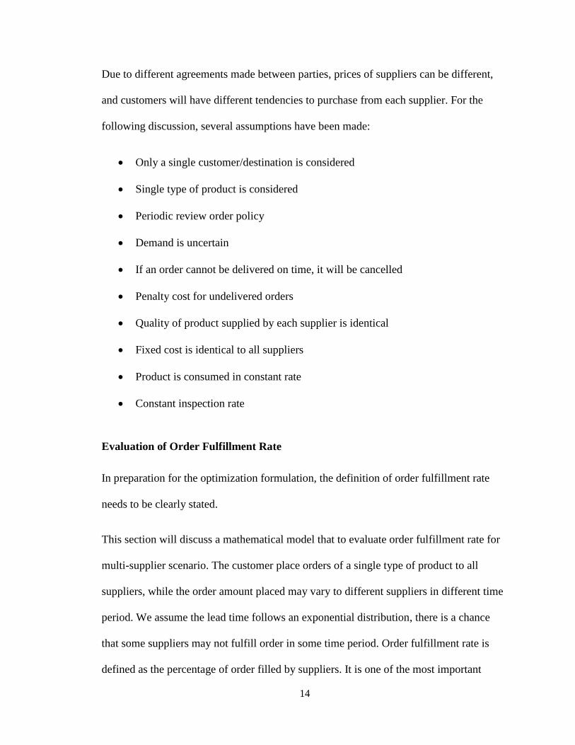
Due to different agreements made between parties, prices of suppliers can be different,
and customers will have different tendencies to purchase from each supplier. For the
following discussion, several assumptions have been made:
Only a single customer/destination is considered
Single type of product is considered
Periodic review order policy
Demand is uncertain
If an order cannot be delivered on time, it will be cancelled
Penalty cost for undelivered orders
Quality of product supplied by each supplier is identical
Fixed cost is identical to all suppliers
Product is consumed in constant rate
Constant inspection rate
Evaluation of Order Fulfillment Rate
In preparation for the optimization formulation, the definition of order fulfillment rate
needs to be clearly stated.
This section will discuss a mathematical model that to evaluate order fulfillment rate for
multi-supplier scenario. The customer place orders of a single type of product to all
suppliers, while the order amount placed may vary to different suppliers in different time
period. We assume the lead time follows an exponential distribution, there is a chance
that some suppliers may not fulfill order in some time period. Order fulfillment rate is
defined as the percentage of order filled by suppliers. It is one of the most important

15
indicators in measuring supply chain performance. Companies that boast some of the
highest order fulfillment rate carry less inventory, experience shorter cash-to-cash cycle
times, and have significantly fewer stock-outs than their competitors; while low
fulfillment rate leads to extra labor costs and administration cost, increased need to
provide replacement orders, low operation efficiency and low customer satisfaction.
Lead time is a time gap between order placement and order receipt. In reality, there
always is latency between the initiation and execution of a process. In the realm of supply
chain management, a company must consider lead time as a vital factor when managing
inventory. If not well-planned, shortage may occur during the delay. Assume the lead
time Lj for the order placed to supplier j follows an exponential distribution with rate μj,
then the properties of the exponential distribution, the expected value and variance of the
lead time are
j
jLE
1][
2
1][
j
jLVar
The purchasing process we discussed uses period review order policy, with time period
length τ. An order is placed by customer at the beginning of the period, and the ordered
product is received by customer by the end of the same period – if the supplier is able to
fulfill the order. For an order placed at the beginning of the time period t, the supplier
may or may not fulfill the order at the end of time period t. Therefore the customer will
either receive an amount of Djt or 0 iterms by the end of period t from supplier j.

16
Let τ be the time length of each period t. The probability that supplier j will successfully
deliver an amount of Djt by the end of period t is
jeLp j
1)(
Define a discrete random variable Yj that represent the order fulfillment rate or the
percentage of the order received from supplier j. For the scenario of single supplier, the
order is either entirely fulfilled or not fulfilled at all. The distribution of order fulfillment
rate Y1 depending on lead time is
1
1
)( 0
1)( 1
1
1
1eLp
eLpY
For the scenario of multiple suppliers, 10 jY , 10 Jj
jY .
1
1
)( 0
1)(
eLp
eLpD
D
Y
j
j
Jj
jt
jt
j
As there are multiple suppliers to whom the customer can place order, we define two sets
M and N as two subsets of supplier set J.
M the set of m suppliers that successfully deliver product by the end of same period t,
JM
N the set of n suppliers that failed to deliver product by the end of same period t,
JN , JNM and NM

17
Then the probability that m suppliers will deliver their orders on time is
Mj Nj
jj eemNp )()1())((
The number of order arrivals by the end of period t depends on the subset M representing
those suppliers capable to deliver order of amount of Djt.
A counting process is used to count the total number of order arrivals from supplier set M.
A compound Poisson process is used to model total order fulfillment rate Y.
Mj
jYY
Within the whole set of suppliers J, each supplier experiences risk of not being able to
fulfill order, then there are nm2 possible combinations of available and unavailable
suppliers in each period t. For each scenario k among all nm2 possible combinations, we
have
Mj
jkk YY
The expected total order fulfillment rate is
nm
k Mj
jk
nm
k
k
nmnm
YY
YE
22
][
2
1
2
1
And the variance of total order fulfillment rate is
22])[(][)( YEYEYVar

18
Optimization Model Formulation
Order fulfillment rate has been defined in previous section and the definition of total cost
is straight forward. In this section the multi-objective optimization problem is formulated.
Sets
In preparation for the formulation, the following sets are identified.
T time period with index t, and time length τ for each period
J supplier with index j
M supplier subset of which can successfully deliver order with indicator mjt
Parameters
A the total cost which involves inventory holding cost for both suppliers and
destination, purchasing cost, inspection cost, and transportation cost.
B the total order fulfillment rate calculated by the ratio of amount successfully
delivered and total amount ordered.
ht inventory holding cost per product unit in period t at the destination
φjt unit purchasing cost from supplier j in period t
βjt unit transportation cost in period t from supplier j to the destination
λjt unit inspection cost in terms of quantity ordered from supplier j in period t
ηt unit penalty cost for undelivered order in period t
19
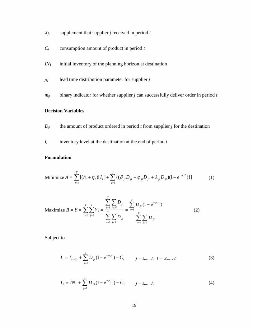
Xjt supplement that supplier j received in period t
Ct consumption amount of product in period t
IN1 initial inventory of the planning horizon at destination
μj lead time distribution parameter for supplier j
mjt binary indicator for whether supplier j can successfully deliver order in period t
Decision Variables
Djt the amount of product ordered in period t from supplier j for the destination
It inventory level at the destination at the end of period t
Formulation
Minimize A =
T
t
J
j
jtjtjtjtjtjtttt
jeDDDIh1 1
)}]1)({(])[[(
(1)
Maximize B = Y =
T
t
J
j
jY1 1
=
T
t Jj
jt
T
t Mj
jt
D
D
1
1=
T
t Jj
jt
T
t
jt
D
eD j
1
1
)1(
(2)
Subject to
t
J
j
jttt CeDII j
1
)1( )1(
;,...,1 Jj Tt ,...,2 (3)
1
1
111 )1( CeDINIJ
j
j
j
;,...,1 Jj (4)
20
t
J
j
jt CeD j
1
)1(
Tt ,...,2 (5)
0,, jttjt IID
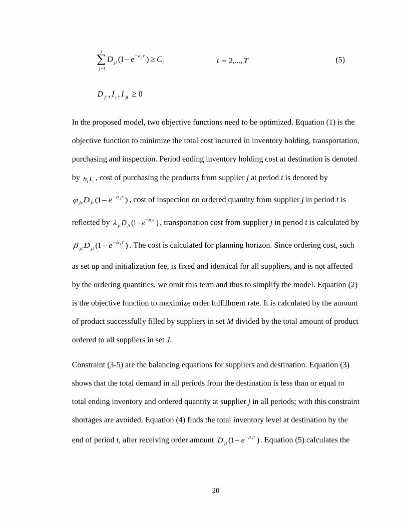
In the proposed model, two objective functions need to be optimized. Equation (1) is the
objective function to minimize the total cost incurred in inventory holding, transportation,
purchasing and inspection. Period ending inventory holding cost at destination is denoted
by tt Ih , cost of purchasing the products from supplier j at period t is denoted by
)1(
jeD jtjt
, cost of inspection on ordered quantity from supplier j in period t is
reflected by )1(
jeD jtjt
, transportation cost from supplier j in period t is calculated by
)1(
jeD jtjt
. The cost is calculated for planning horizon. Since ordering cost, such
as set up and initialization fee, is fixed and identical for all suppliers, and is not affected
by the ordering quantities, we omit this term and thus to simplify the model. Equation (2)
is the objective function to maximize order fulfillment rate. It is calculated by the amount
of product successfully filled by suppliers in set M divided by the total amount of product
ordered to all suppliers in set J.
Constraint (3-5) are the balancing equations for suppliers and destination. Equation (3)
shows that the total demand in all periods from the destination is less than or equal to
total ending inventory and ordered quantity at supplier j in all periods; with this constraint
shortages are avoided. Equation (4) finds the total inventory level at destination by the
end of period t, after receiving order amount )1( jeD jt
. Equation (5) calculates the

21
total inventory level at the destination by the end of 1st period, after receiving order
amount )1(1
jeD j
.
Numerical Example
To further illustrate above problem, a numerical example is presented. We run empirical
data in Excel Spreadsheet.
We assume a scenario of four suppliers and ten months.

22
Month It Djt
η
($) ht ($) φjt ($) βjt ($)
1 2 3 4 1 2 3 4 1 2 3 4
1 102.8174 120 110 120 120 20 5 21 27 29 19 9 7 6 10
2 152.8511 115 105 125 110 20 5 22 26 29 19 10 7 8 10
3 213.1002 115 105 120 115 20 5 23 25 28 18 8 8 10 10
4 245.7022 120 110 125 115 20 5 23 24 29 20 7 8 12 10
5 308.3041 120 110 125 115 20 5 25 34 22 25 9 6 14 10
6 352.6882 115 105 125 115 20 5 28 30 26 28 12 6 6 9
7 395.4491 125 105 125 115 20 5 22 31 27 29 15 6 7 9
8 476.4278 130 110 125 115 20 5 29 32 33 36 4 6 8 11
9 534.8414 115 110 125 115 20 5 19 21 32 19 6 9 9 11
10 583.2549 115 110 125 115 20 5 28 21 30 15 12 7 10 12
λjt ($) Xjt Ct INj1 IN1 μj
1 2 3 4 1 2 3 4 1 2 3 4 1 2 3 4
1 1 1 1 100 95 120 100 350
50 50 60 50 60 1.818182 1.639344 1.754386 2.040816
1 1 1 1 100 85 110 100 330
1 1 1 1 100 90 115 100 320
1 1 1 1 120 100 110 100 360
1 1 1 1 90 95 110 100 330
1 1 1 1 95 95 100 100 340
1 1 1 1 105 95 105 110 350
1 1 1 1 110 90 110 110 320
1 1 1 1 115 95 105 90 330
1 1 1 1 100 100 110 90 340
Table 1. Numerical Example Parameters
23
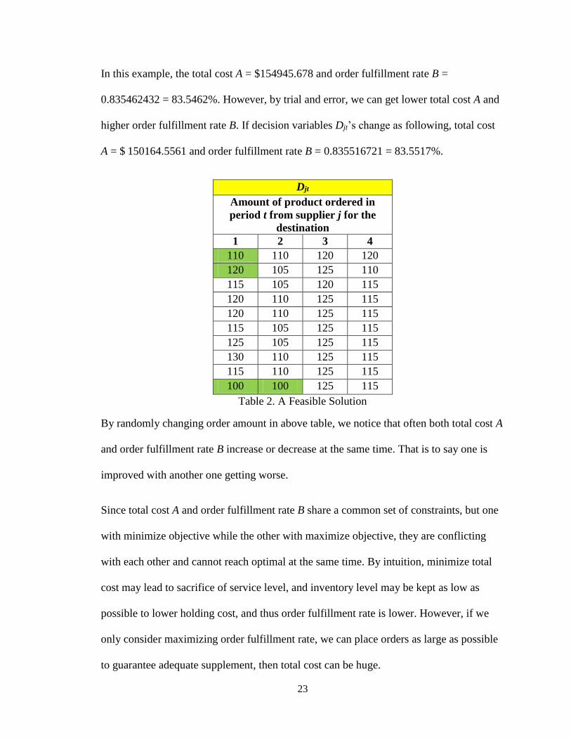
In this example, the total cost A = $154945.678 and order fulfillment rate B =
0.835462432 = 83.5462%. However, by trial and error, we can get lower total cost A and
higher order fulfillment rate B. If decision variables Djt’s change as following, total cost
A = $ 150164.5561 and order fulfillment rate B = 0.835516721 = 83.5517%.
Djt
Amount of product ordered in
period t from supplier j for the
destination
1 2 3 4
110 110 120 120
120 105 125 110
115 105 120 115
120 110 125 115
120 110 125 115
115 105 125 115
125 105 125 115
130 110 125 115
115 110 125 115
100 100 125 115
Table 2. A Feasible Solution
By randomly changing order amount in above table, we notice that often both total cost A
and order fulfillment rate B increase or decrease at the same time. That is to say one is
improved with another one getting worse.
Since total cost A and order fulfillment rate B share a common set of constraints, but one
with minimize objective while the other with maximize objective, they are conflicting
with each other and cannot reach optimal at the same time. By intuition, minimize total
cost may lead to sacrifice of service level, and inventory level may be kept as low as
possible to lower holding cost, and thus order fulfillment rate is lower. However, if we
only consider maximizing order fulfillment rate, we can place orders as large as possible
to guarantee adequate supplement, then total cost can be huge.

24
Chapter 4
Optimization of Performance Measures
This chapter describes three commonly used methods/tools for optimization problem.
The problem is at first solved by Excel Solver, but the results are not desirable. Then
Interior-Point method and Augmented Simultaneous Perturbation Stochastic
Approximation (ASPSA) method are used to solve the problem. Both of them are coded
by using Matlab. Then a comparison is presented among them.
Excel Solver VBA
To solve the optimization problem, we first use an embedded function in Excel. A set of
VBA program utilizing Solver function is written for solving the problem. We played
with the VBA program, and noticed that the optimal results slightly changed, either up or
down, after every run trial. E.g., for total cost A the optimum varies between $120,000-
ish and $170,000-ish. Without changing problem constraints, we change initial values of
decision variables each time, and found that the results are highly correlated to initial
values input. One of the best results we got from VBA program is shown in the table
below.
Min Total Cost A = $ 121,886.1527 with B = 0.835493289
It Djt
54.73772 106.2516 95.05023 104.2169 106.8258
54.99999 100.3561 90.48099 108.3328 96.18491
65.91539 100.8109 90.48777 102.8977 101.6573
47.99983 106.2586 95.91853 106.5716 100.7272
55.61136 104.4676 92.47244 108.7818 98.40182

25
44.79612 96.78111 89.19549 110.55 97.47168
31.99999 108.1244 88.76473 109.6659 97.00661
52.38973 114.92 93.33846 106.5762 92.82585
62.87101 103.5021 96.78455 106.5762 100.732
60 96.78578 97.64608 107.0183 102.1272
Table 3. VBA Result for Optimizing A
Max Order Fulfillment Rate B = 0.870077392 with A = $ 169644.424
It Djt
2673.943 0 0 0 3406.528
2343.943 0 0 0 0
2045.232 0 0 0 24.46826
1717.37 0 0 0 36.93648
1474.982 0 0 0 100.6952
1134.982 0 0 0 0
821.6534 0 0 0 42.14696
589.9975 0 0 0 101.5358
359.2216 0 0 0 114.0405
60 0 0 0 46.86759
Table 4. VBA Result for Optimizing B
We also noticed a problem that if consider integer constraints for decision variables
(since they denote product item volume), the VBA program will take a very long time to
run (more than 15 minutes) and may not always reach an optimum eventually.
After a lot of tests, we found the optima of each test were not identical. One of the main
reasons is the initial values of decision variables. We observed that the optima of both
performance A and B vary with the change of initial value of Djt and It. We were also
aware of low efficiency of the program.
The VBA code is shown is Appendix A.

26
Due to the limitation of Solver function embedded in Excel, we then convert to more
powerful tools for problem solving.
Interior-Point Method
An Interior-Point method is a linear or nonlinear programming method that combines the
advantages of the simplex algorithm with the geometry of the ellipsoid algorithm that
achieves optimization.
Convex program with inequality:
Minimize f0(x)
Subject to fi(x) ≤ 0, i = 1,…, m
Ax = b
where
f0,…,fm: Rn → R convex, twice differentiable
A ∈ Rp×n with rank p < n
An optimal x* exists
The pseudo code of the process is shown below.
given strictly feasible x, t := t(0) > 0, μ >1, tolerance ε > 0.
repeat
Centering step. Compute x*(t) by minimizing tf0+ϕ, subject to Ax = b.
Update x := x*(t).
Stopping criterion. quit if m/t < ε.
Increase t. t := μt.

27
We implemented the logic by using Matlab. The optimal solutions for total cost and
fulfillment rate are shown below.
Min Total Cost A = $ 105,020 with B = 0.8479
It Djt
0 0 0 0 333
0 0 0 0 379
0 0 0 0 368
0 215 0 0 207
0 394 0 0 0
0 0 0 411 0
0 0 0 423 0
0 382 0 0 0
0 394 0 0 0
60 0 0 0 460
Table 5. Interior-Point Method for Optimizing A
Max Order Fulfillment Rate B = 0.8701 with A = $ 107,091.6768
It Djt
70 0 0 0 360
100 0 0 0 360
140 0 0 0 360
140 0 0 0 360
170 0 0 0 360
190 0 0 0 360
201 0 0 0 360
242 0 0 0 361
274 0 0 0 363
301 0 0 0 367
Table 6. Interior-Point Method for Optimizing B
The Matlab code using Interior-Point method and fmincon function is shown in Appendix
A.

28
Augmented Simultaneous Perturbation Stochastic Approximation (ASPSA) method
ASPSA method is an improvement of SPSA. It incorporated techniques including ordinal
optimization (OO), pre-search, line search memory of best solution, and non-uniform step
size gain. ASPSA not only achieves speed up, but also improves solution quality and
converges faster than SPSA.
________________________________________________________________________
ASPSA Algorithm (Wang and Prabhu, 2009)
Step 1. Initialization and coefficient selection
Set counter index k = 0, ck = c and distribution for ak.
Step 2. Presearch
Randomly choose θj(j = 1, ... m) from the decision space;
Evaluating them by running simulation in ns length;
Let yb = min{yj, j = 1, ..., m};
Run full simulation length to evaluate y(θb);
Set θbest = θk = θb, ybest = yb.
Step 3. Generate simultaneous perturbation vector Δk
Step 4. Loss function evaluation
Order y(θk + ckΔk) and y(θk - ckΔk) by evaluating them in length of ns
Step 5. Gradient approximation
otherwise 1
)()( if 1
k
kkkk
kk
cycy
g

29
Step 6. Line search
Generate step size vector akj (j = 1,…,l) from some random distribution;
Calculate k
j
k
j
k
j
k ga
1, j = 1, …, l
Evaluate y(θk+1j) in short simulation length ns
Let yb = min{Jj, j = 1, ..., l};
Run full simulation length to reevaluate y(θb);
If ybest > yb, ybest = yb and θbest = θk+1 = θb;
Otherwise, θk+1 = θbest + Λk where Λk is a perturbation vector
Step 7. Iteration or termination
k ← k +1. If stop criteria is satisfied, stop. Otherwise, go to step 2.
________________________________________________________________________
Referring to Wang and Spall (2008), we use the following parameter values:
an = 0.1(n+100)-0.602 and cn = n-0.101
The ASPSA method is also coded in Matlab. We played with the program by changing
number of iterations. Shown in Figure 8, as the number of iterations increases, the
decrease of optimal value of objective A becomes slowly. If we set 150,000 iterations, the
following results are achieved.
Min Total Cost A = $ 111,320 with B = 0.838517319
It Djt
0.2307 88.92506 22.67039 0 227.2314
0.3787 90.52844 114.4733 0 187.0396
16.3164 133.8396 45.79779 0 215.1398
85.3308 168.1548 168.2569 0 176.4629

30
56.4482 151.6375 26.52388 120.0213 61.54234
87.8982 20.47216 139.1411 250.4327 40.72305
67.9389 82.77013 73.7329 196.3757 44.37835
0 248.6775 54.36506 0.233377 0
117.8519 249.5694 147.0041 0 139.1369
58.0089 0 181.2779 0.104234 154.4148
Table 7. ASPSA Method for Optimizing A
(For convenience, all numbers are rounded to 0 if less than 1)
Max Order Fulfillment Rate B = 0.8346 with A = $ 115,559.6172
It Djt
70.02639 90.11218 89.59581 89.86332 90.45029
100.027 90.04207 89.63968 89.89583 90.42298
139.9975 90.01394 89.61568 89.98122 90.35754
139.9934 90.11478 89.58598 89.85059 90.44157
170.0507 90.01233 89.61557 89.98932 90.43565
190.0195 90.09954 89.58275 89.89885 90.38792
199.9659 90.02699 89.64454 89.8304 90.44283
240.0607 90.09323 89.66048 89.95461 90.39001
270.0003 90.03551 89.6264 89.92862 90.35212
290.0178 90.03119 89.57264 89.95698 90.45762
Table 8. ASPSA Method for Optimizing B
Figure 7. The change of 50 variables for 150000 iterations for maximizing A

31
Figure 8. The change of objective A for 150000 iterations
Figure 9. The change of 50 variables for 150000 iterations for minimizing B

32
Figure 10. The change of objective B for 150000 iterations
A Comparison between VBA and Matlab
Since VBA is embedded in MS Excel and all data are stored in the spreadsheet, it is the
most convenient tool on hand to use for optimization by simply enables Macros. The
VBA code is also easy to understand and write, with a lot of open sources online to refer
to. However, by using VBA Solver we don't know the exact algorithm it utilized to do
optimization. We did try to realize other optimization algorithms in VBA, but it is hard to
debug compare with other programming languages. Matlab is another commonly used
programming language. We then converted to use Matlab to realize algorithms.
A Comparison between Interior Point Method and ASPSA Method
Under current situation, the elapsed time for each method is shown below:
33
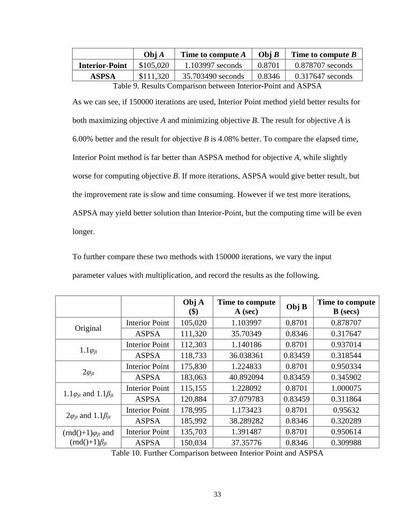
Obj A Time to compute A Obj B Time to compute B
Interior-Point $105,020 1.103997 seconds 0.8701 0.878707 seconds
ASPSA $111,320 35.703490 seconds 0.8346 0.317647 seconds
Table 9. Results Comparison between Interior-Point and ASPSA
As we can see, if 150000 iterations are used, Interior Point method yield better results for
both maximizing objective A and minimizing objective B. The result for objective A is
6.00% better and the result for objective B is 4.08% better. To compare the elapsed time,
Interior Point method is far better than ASPSA method for objective A, while slightly
worse for computing objective B. If more iterations, ASPSA would give better result, but
the improvement rate is slow and time consuming. However if we test more iterations,
ASPSA may yield better solution than Interior-Point, but the computing time will be even
longer.
To further compare these two methods with 150000 iterations, we vary the input
parameter values with multiplication, and record the results as the following.
Obj A
($)
Time to compute
A (sec) Obj B
Time to compute
B (secs)
Original Interior Point 105,020 1.103997 0.8701 0.878707
ASPSA 111,320 35.70349 0.8346 0.317647
1.1φjt Interior Point 112,303 1.140186 0.8701 0.937014
ASPSA 118,733 36.038361 0.83459 0.318544
2φjt Interior Point 175,830 1.224833 0.8701 0.950334
ASPSA 183,063 40.892094 0.83459 0.345902
1.1φjt and 1.1βjt Interior Point 115,155 1.228092 0.8701 1.000075
ASPSA 120,884 37.079783 0.83459 0.311864
2φjt and 1.1βjt Interior Point 178,995 1.173423 0.8701 0.95632
ASPSA 185,992 38.289282 0.8346 0.320289
(rnd()+1)φjt and
(rnd()+1)βjt
Interior Point 135,703 1.391487 0.8701 0.950614
ASPSA 150,034 37.35776 0.8346 0.309988
Table 10. Further Comparison between Interior Point and ASPSA
34
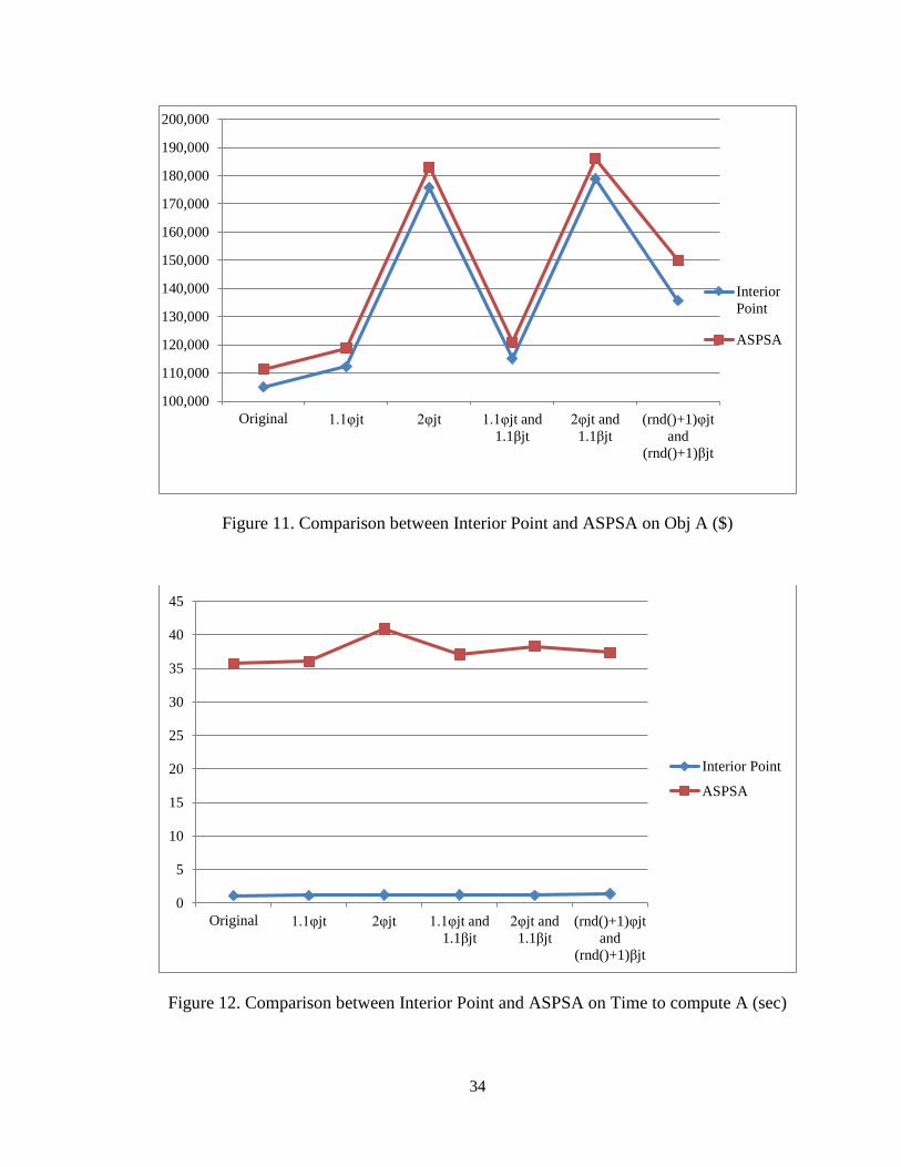
Figure 11. Comparison between Interior Point and ASPSA on Obj A ($)
Figure 12. Comparison between Interior Point and ASPSA on Time to compute A (sec)
100,000
110,000
120,000
130,000
140,000
150,000
160,000
170,000
180,000
190,000
200,000
Original 1.1φjt 2φjt 1.1φjt and
1.1βjt
2φjt and
1.1βjt
(rnd()+1)φjt
and
(rnd()+1)βjt
Interior
Point
ASPSA
0
5
10
15
20
25
30
35
40
45
Original 1.1φjt 2φjt 1.1φjt and
1.1βjt
2φjt and
1.1βjt
(rnd()+1)φjt
and
(rnd()+1)βjt
Interior Point
ASPSA

35
Figure 13. Comparison between Interior Point and ASPSA on Obj B
Figure 14. Comparison between Interior Point and ASPSA on Time to compute B (secs)
0.81
0.82
0.83
0.84
0.85
0.86
0.87
0.88
Original 1.1φjt 2φjt 1.1φjt and
1.1βjt
2φjt and
1.1βjt
(rnd()+1)φjt
and
(rnd()+1)βjt
Interior Point
ASPSA
0
0.2
0.4
0.6
0.8
1
1.2
Original 1.1φjt 2φjt 1.1φjt and
1.1βjt
2φjt and
1.1βjt
(rnd()+1)φjt
and
(rnd()+1)βjt
Interior Point
ASPSA

36
We changed unit purchasing cost (φjt) and unit transportation cost (βjt). Five other
scenarios are considered: magnify φjt to its 1.1 multiplications; magnify φjt to its 2
multiplications; magnify φjt to its 1.1 multiplications and βjt to its 1.1 multiplication;
magnify φjt to its 2 multiplications and βjt to its 1.1 multiplications; as well as magnify φjt
to its 1~2 multiplications and βjt to its 1~2 multiplications.
As shown in Table 10, for total cost A, Interior-Point method yields better solution for
4%-10%, and takes much shorter computing time.
For order fulfillment B, the optimal rarely vary for either method. Elapsed times are
shorter for ASPSA, but the differences are not vital since all of them are less than 1
second.

37
Chapter 5
A Multiple Criteria Model to Evaluate Performance Measures
In the problem we discussed above, with the same set of constraints, two objectives are
considered: total cost A and order fulfillment rate B. We want to have both maximized A
as well as minimized B at the same time to meet customer’s satisfaction. So the
relationship between objectives and constraints is not completely solid. Goal
programming method is used to achieve both goals simultaneously. It is a good idea to
treat both of them as constraints by adding slack variables to represent deviation from a
goal.
Goal Programming
(Lawrence and Pasternack, 2002) A goal programming model seeks to simultaneously
consider several objective functions that are in decision makers concern. Compare to a
linear programming model consists a set of constraints and a single objective function to
be maximized or minimized, a goal programming model consists the same set of
constraints, a set of goals that are prioritized in some sense, and a single penalty objective
function to be minimized. The objective is to find a solution that satisfies the true
constraints and comes closest to meeting the stated goals. Here we use optimal values for
each objective function as the stated goals. All objective functions share the same set of
constraints.
Non Preemptive Goal Programming

38
In non-preemptive goal programming, relative weights are assigned to each goal. The
larger the weight value, the more importance the goal is to decision makers. These
weights act as unit penalty that fail to meet a stated goal. The form of non-preemptive
goal programming is:
Minimize the total weighted deviations from the goals
Subject to (1) Expressions for the goal equations
(2) Functional constraints
(3) Non-negativity constraints of all decision and deviation variables
Preemptive Goal Programming
Preemptive goal programming shares the same basic idea with non-preemptive goal
programming that to find the best solution set as close to the stated goals as possible.
However in preemptive goal programming decision makers determine the relative
priority of multiple objective functions. Objective functions, or goals, are prioritized.
Higher prioritized goal must be satisfied before considering lower prioritized ones. (Jones
et al., 1995)
Goal Programming Model
Since both objectives are equally prioritized, decision maker is more interested in direct
comparison of objectives, so non pre-emptive goal programming is used.
Before implementing goal programming, penalties need to be determined for not reaching
a goal. We notice that the result for total cost A is at ×105 order of magnitude and B is at

39
×10-1 order of magnitude. We define the penalties as: for every $ 1,000 that the total cost
exceeds optimal A, pA is penalized; for every 1 percent that order fulfillment rate
decreased compared to optimal B, pB is penalized. To balance their order of magnitude,
here we use
pA = 8 and pB = 10
as an example. These two penalty values vary against specific conditions and
management concerns.
We use the results from Interior Point method as the optimal solutions. Then the goal
programming is formulated as
Minimize Total Penalty = )100(101000
8B
A ss
Subject to
105020 AsA
8701.0 BsB
t
J
j
jttt CeDII j
1
)1( )1(
;,...,1 Jj Tt ,...,2
1
1
111 )1( CeDINIJ
j
j
j
;,...,1 Jj
t
J
j
jt CeD j
1
)1(
Tt ,...,2

40
0,, jttjt IID
0, AsA
1,0 BsB
Again, by using Interior Point method in Matlab, we have the following optimal solution.
It Djt
0 0 0 0 333
0 0 0 0 379
0 0 0 0 368
143 0 0 0 578
0 0 0 0 215
0 0 0 411 0
0 0 0 423 0
0 382 0 0 0
0 394 0 0 0
60 0 0 0 460
Table 11. Goal Programming Results
0.854585
105,349$
0155.0
329
B
A
s
s
B
A
The optimal value of Total Penalty = 18.1463.
To reach the optimal solution, we changed Matlab code of Interior-Point method
accordingly. It is attached in Appendix A.

41
Chapter 6
Conclusions
In previous works, we firstly discussed the expansion of Panama Canal and
corresponding consequences. With the expansion more and more suppliers are directly
available to customers along the East coast and they are facing fiercer competition
against each other. Under this condition, we are interested in the new purchase process
pattern which led by the expansion. In contrast to the sole supplier scenario in the past, a
new scenario of multiple suppliers and single customer is analyzed in the research. By
estimating customer’s concerns, two main performance measures are taken into account
to evaluate the supply chain: total cost A and order fulfillment rate B. An EOQ model is
then established for them. Both of them are formulated with the amount of product
ordered (Djt) and inventory level at the destination (It), as decision variables, and
inventory holding cost (ht), unit purchasing cost (φjt) and product consumption amount
(Ct) etc., as parameters. Our aim is to find a compromising solution that maximize total
cost A and minimize order fulfillment rate B simultaneously.
To solve these two optimization problems, we first considered them separately. VBA
Solver and Matlab are the programming language tools that we used for optimizing the
two problems. In Matlab, two method – Interior-Point method and Augmented
Simultaneous Perturbation Stochastic Approximation (ASPSA) method are realized.
Comparisons between VBA Solver and Matlab, as well as Interior-Point method and
ASPSA method are then presented. We conclude that Interior-Point method is better for
generating ideal results and shorter computing time for the problem we discuss.

42
As the optimal solutions for both A and B are found, we integrate them into a single
model so that a compromising solution can be found. Non pre-emptive goal programming
technique is used. A compromising solution is reached with corresponding penalties.
We proposed possible methods for customer to evaluate suppliers on the aspect of total
cost and order fulfillment rate. For the final selection process, goal programming method
was recommended. An example and its corresponding solutions were presented to further
illustrate the ideas.
43
Appendix A
VBA Code
Sub multiob()
Worksheets("find").Activate
Dim initiala As Long
initiala = 200000
Dim initialb As Integer
initialb = 0.1
Range("$I$18").Value = initiala
Range("$J$18").Value = initialb
Range("$K$18").Value = initiala
Range("$L$18").Value = initialb
Dim i As Integer
For i = 1 To 10
' Min A
SolverReset
SolverOk SetCell:=Range("$D$17"), MaxMinVal:=2, ValueOf:="0",
ByChange:="$B$4:$B$13,$E$4:$H$13"
SolverAdd CellRef:=Range("$D$21:$D$30"), Relation:=2,
FormulaText:=Range("$F$21:$F$30")
SolverAdd CellRef:=Range("$D$31"), Relation:=3,
FormulaText:=Range("$F$31")
' It takes a long time to run if the following two constraints
are considered
' SolverAdd CellRef:=Range("$B$4:$B$13"), Relation:=4
' SolverAdd CellRef:=Range("$E$4:$H$13"), Relation:=4
SolverSolve userFinish:=True
If Range("$D$17") < Range("$I" & i + 17) Then
Range("$M$18:$M$27").Value = Range("$B$4:$B$13").Value
Range("$N$18:$Q$27").Value = Range("$E$4:$H$13").Value
End If
Range("$I" & i + 17).Value = Range("$D$17")
Range("$J" & i + 17).Value = Range("$F$17")
' Max B
SolverReset
SolverOk SetCell:=Range("$F$17"), MaxMinVal:=1, ValueOf:="0",
ByChange:="$B$4:$B$13,$E$4:$H$13"
SolverAdd CellRef:=Range("$D$21:$D$30"), Relation:=2,
FormulaText:=Range("$F$21:$F$30")
SolverAdd CellRef:=Range("$D$31"), Relation:=3,
FormulaText:=Range("$F$31")

44
' It takes a long time to run if the following two constraints
are considered
' SolverAdd CellRef:=Range("$B$4:$B$13"), Relation:=4
' SolverAdd CellRef:=Range("$E$4:$H$13"), Relation:=4
SolverSolve userFinish:=True
If Range("$F$17") > Range("$L" & i + 17) Then
Range("$R$18:$R$27").Value = Range("$B$4:$B$13").Value
Range("$S$18:$V$27").Value = Range("$E$4:$H$13").Value
End If
Range("$K" & i + 17).Value = Range("$D$17")
Range("$L" & i + 17).Value = Range("$F$17")
Next
End Sub
Interior-Point Method
Main solver for both optimizing total cost A and order fulfillment B:
%% Clear environments
clear all; close all; clc;
%% Prepare Constants
parameter.ht = 5*ones(10, 1);
parameter.beta = [9 7 6 10;
10 7 8 10;
8 8 10 10;
7 8 12 10;
9 6 14 10;
12 6 6 9;
15 6 7 9;
4 6 8 11;
6 9 9 11;
12 7 10 12];
parameter.lambda = ones(10,4);
parameter.phi = [21 27 29 19;
22 26 29 19;
23 25 28 18;
23 24 29 20;
25 34 22 25;
28 30 26 28;
22 31 27 29;
29 32 33 36;
19 21 32 19;
28 21 30 15];

45
parameter.c = [350;
330;
320;
360;
330;
340;
350;
320;
330;
340];
parameter.miu = [1.818181818 1.639344262 1.754385965
2.040816327]';
parameter.in = [60 0 0 0 0 0 0 0 0 0]';
parameter.Mat = [1 0 0 0 0 0 0 0 0 0;
-1 1 0 0 0 0 0 0 0 0;
0 -1 1 0 0 0 0 0 0 0;
0 0 -1 1 0 0 0 0 0 0;
0 0 0 -1 1 0 0 0 0 0;
0 0 0 0 -1 1 0 0 0 0;
0 0 0 0 0 -1 1 0 0 0;
0 0 0 0 0 0 -1 1 0 0;
0 0 0 0 0 0 0 -1 1 0;
0 0 0 0 0 0 0 0 -1 1];
% Lower bound
lb = zeros(50, 1);
% Initial value x0
x0 = [70 100 140 140 170 190 200 240 270 290 90*ones(1, 40)]';
%% Execute fmincon with ObjA
options_A = optimset('Algorithm', 'active-set', 'MaxFunEvals',
100000, 'MaxIter', 10000, 'Display', 'off');
[x,fval,exitflag,output,lambda,grad] =
fmincon(@(x)ObjectiveA(x,parameter),x0,[],[],[],[],lb,[],@(x)Cons
tra(x, parameter), options_A);
%% Execute fmincon with ObjB
options_B = optimset('Algorithm', 'active-set', 'MaxFunEvals',
100000, 'MaxIter', 10000, 'Display', 'off');
[x,fval,exitflag,output,lambda,grad] =
fmincon(@(x)ObjectiveB(x,parameter),x0,[],[],[],[],lb,[],@(x)Cons
tra(x, parameter), options_B);
real_fval = 1/(fval/10000);
Constraints.m
% Input x format:
% 01 - 10: Column B
% 11 - 20: Column I
% 21 - 30: Column J
% 31 - 40: Column K

46
% 41 - 50: Column L
function [ c, ceq ] = Constra( x, parameter )
% Decomposition to vector
b = x(1:10, 1);
e_1 = x(11:20, 1);
e_2 = x(21:30, 1);
e_3 = x(31:40, 1);
e_4 = x(41:50, 1);
% Compute inequal constraint
c = sum(parameter.c) - sum(e_1) - sum(e_2) - sum(e_3) - sum(e_4);
% Compute equal constraint
ceq = parameter.Mat*b - e_1 - e_2 - e_3 - e_4 - parameter.in +
parameter.c;
end
ObjectiveA.m
% Input x format:
% 01 - 10: Column B
% 11 - 20: Column I
% 21 - 30: Column J
% 31 - 40: Column K
% 41 - 50: Column L
function ObjA = ObjectiveA( x, parameter )
% Decomposition to vector
b = x(1:10, 1);
e_1 = x(11:20, 1);
e_2 = x(21:30, 1);
e_3 = x(31:40, 1);
e_4 = x(41:50, 1);
% Compute ObjectiveA value
ObjA = 0;
ObjA = ObjA + parameter.ht'*b;
ObjA = ObjA + parameter.beta(:,1)'*e_1 + parameter.beta(:,2)'*e_2
+ parameter.beta(:,3)'*e_3 + parameter.beta(:,4)'*e_4;
ObjA = ObjA + parameter.phi(:,1)'*e_1 + parameter.phi(:,2)'*e_2 +
parameter.phi(:,3)'*e_3 + parameter.phi(:,4)'*e_4;
ObjA = ObjA + parameter.lambda(:,1)'*e_1 +
parameter.lambda(:,2)'*e_2 + parameter.lambda(:,3)'*e_3 +
parameter.lambda(:,4)'*e_4;
End
ObjectiveB.m

47
% Input x format:
% 01 - 10: Column B
% 11 - 20: Column I
% 21 - 30: Column J
% 31 - 40: Column K
% 41 - 50: Column L
function ObjB = ObjectiveB( x, parameter )
% Decomposition to vector
e_1 = x(11:20, 1);
e_2 = x(21:30, 1);
e_3 = x(31:40, 1);
e_4 = x(41:50, 1);
% Compute ObjectiveBvalue
temp_1 = sum(e_1/(1 - exp(-parameter.miu(1))));
temp_1 = temp_1 + sum(e_2/(1 - exp(-parameter.miu(2))));
temp_1 = temp_1 + sum(e_3/(1 - exp(-parameter.miu(3))));
temp_1 = temp_1 + sum(e_4/(1 - exp(-parameter.miu(4))));
temp_2 = sum(e_1) + sum(e_2) + sum(e_3) + sum(e_4);
ObjB = 10000*temp_1/temp_2;
end
ASPSA Method
ASPSA_ObjA.m
clear all
close all
clc
% Prepare Constants
parameter.ht = 5*ones(10, 1);
parameter.beta = [9 7 6 10;
10 7 8 10;
8 8 10 10;
7 8 12 10;
9 6 14 10;
12 6 6 9;
15 6 7 9;
4 6 8 11;
6 9 9 11;
12 7 10 12];
parameter.lambda = ones(10,4);
parameter.phi = [21 27 29 19;
22 26 29 19;
23 25 28 18;
23 24 29 20;
25 34 22 25;
48
28 30 26 28;
22 31 27 29;
29 32 33 36;
19 21 32 19;
28 21 30 15];
parameter.c = [350;
330;
320;
360;
330;
340;
350;
320;
330;
340];
parameter.miu = [1.818181818 1.639344262 1.754385965
2.040816327]';
parameter.in = [60 0 0 0 0 0 0 0 0 0]';
parameter.Mat = [1 0 0 0 0 0 0 0 0 0;
-1 1 0 0 0 0 0 0 0 0;
0 -1 1 0 0 0 0 0 0 0;
0 0 -1 1 0 0 0 0 0 0;
0 0 0 -1 1 0 0 0 0 0;
0 0 0 0 -1 1 0 0 0 0;
0 0 0 0 0 -1 1 0 0 0;
0 0 0 0 0 0 -1 1 0 0;
0 0 0 0 0 0 0 -1 1 0;
0 0 0 0 0 0 0 0 -1 1];
%Reserve Space for x
n = 150000;
x = zeros(50, n);
ObjValue = zeros(1,n);
% Initial value x0
x(:,1) = [70 100 140 140 170 190 200 240 270 290 90*ones(1, 40)]';
ObjValue(1) = newObjectiveA(x(:,1), parameter);
% Equality
cgrad=[1 0 0 0 0 0 0 0 0 0 -1 0 0 0 0 0 0 0 0 0 -1 0 0 0 0 0 0 0
0 0 -1 0 0 0 0 0 0 0 0 0 -1 0 0 0 0 0 0 0 0 0;
-1 1 0 0 0 0 0 0 0 0 0 -1 0 0 0 0 0 0 0 0 0 -1 0 0 0 0 0 0 0 0 0
-1 0 0 0 0 0 0 0 0 0 -1 0 0 0 0 0 0 0 0;
0 -1 1 0 0 0 0 0 0 0 0 0 -1 0 0 0 0 0 0 0 0 0 -1 0 0 0 0 0 0 0 0
0 -1 0 0 0 0 0 0 0 0 0 -1 0 0 0 0 0 0 0;
0 0 -1 1 0 0 0 0 0 0 0 0 0 -1 0 0 0 0 0 0 0 0 0 -1 0 0 0 0 0 0 0
0 0 -1 0 0 0 0 0 0 0 0 0 -1 0 0 0 0 0 0;
0 0 0 -1 1 0 0 0 0 0 0 0 0 0 -1 0 0 0 0 0 0 0 0 0 -1 0 0 0 0 0 0
0 0 0 -1 0 0 0 0 0 0 0 0 0 -1 0 0 0 0 0;
0 0 0 0 -1 1 0 0 0 0 0 0 0 0 0 -1 0 0 0 0 0 0 0 0 0 -1 0 0 0 0 0
0 0 0 0 -1 0 0 0 0 0 0 0 0 0 -1 0 0 0 0;
0 0 0 0 0 -1 1 0 0 0 0 0 0 0 0 0 -1 0 0 0 0 0 0 0 0 0 -1 0 0 0 0
0 0 0 0 0 -1 0 0 0 0 0 0 0 0 0 -1 0 0 0;

49
0 0 0 0 0 0 -1 1 0 0 0 0 0 0 0 0 0 -1 0 0 0 0 0 0 0 0 0 -1 0 0 0
0 0 0 0 0 0 -1 0 0 0 0 0 0 0 0 0 -1 0 0;
0 0 0 0 0 0 0 -1 1 0 0 0 0 0 0 0 0 0 -1 0 0 0 0 0 0 0 0 0 -1 0 0
0 0 0 0 0 0 0 -1 0 0 0 0 0 0 0 0 0 -1 0;
0 0 0 0 0 0 0 0 -1 1 0 0 0 0 0 0 0 0 0 -1 0 0 0 0 0 0 0 0 0 -1 0
0 0 0 0 0 0 0 0 -1 0 0 0 0 0 0 0 0 0 -1]';
% Inequality
qgrad=[0 0 0 0 0 0 0 0 0 0 -1 -1 -1 -1 -1 -1 -1 -1 -1 -1 -1 -1 -1
-1 -1 -1 -1 -1 -1 -1 -1 -1 -1 -1 -1 -1 -1 -1 -1 -1 -1 -1 -1 -1 -1
-1 -1 -1 -1 -1]';
% Calculate g(x)
for i = 1:1:n-1
a = 0.1*(i+100)^(-0.602);
r = 10*i^(0.1);
c = i^(-0.101);
delta = 2*round(rand(50,1))-1;
% Calculate ghat
gplus = newObjectiveA(x(:,i)+c*delta, parameter);
gminus = newObjectiveA(x(:,i)-c*delta, parameter);
ghat = (gplus - gminus)/(2*c)./delta;
% Calculate P3
MinMatrix = [zeros(50,1) x(:,i)];
MinVector = min(MinMatrix')';
% Calculate next step
x(:,(i+1)) = x(:,i) - a*ghat - a*r*(cgrad*Ceq(x(:,i),
parameter)+qgrad*max(0,Cineq(x(:,i), parameter))+MinVector);
ObjValue(i+1) = newObjectiveA(x(:,i+1), parameter);
end
index = 1:1:n;
figure
plot(index, ObjValue);
grid on;
figure
plot(index, x);
grid on;
newObjectiveA.m
% Input x format:
% 01 - 10: Column B
% 11 - 20: Column I
% 21 - 30: Column J
% 31 - 40: Column K
% 41 - 50: Column L
function ObjA = newObjectiveA( x, parameter )
% Decomposition to vector

50
b = x(1:10, 1);
e_1 = x(11:20, 1);
e_2 = x(21:30, 1);
e_3 = x(31:40, 1);
e_4 = x(41:50, 1);
% Compute ObjectiveA value
ObjA = 0;
ObjA = ObjA + parameter.ht'*b;
ObjA = ObjA + parameter.beta(:,1)'*e_1 + parameter.beta(:,2)'*e_2
+ parameter.beta(:,3)'*e_3 + parameter.beta(:,4)'*e_4;
ObjA = ObjA + parameter.phi(:,1)'*e_1 + parameter.phi(:,2)'*e_2 +
parameter.phi(:,3)'*e_3 + parameter.phi(:,4)'*e_4;
ObjA = ObjA + parameter.lambda(:,1)'*e_1 +
parameter.lambda(:,2)'*e_2 + parameter.lambda(:,3)'*e_3 +
parameter.lambda(:,4)'*e_4;
end
ASPSA_ObjB.m
clear all
close all
clc
% Prepare Constants
parameter.ht = 5*ones(10, 1);
parameter.beta = [9 7 6 10;
10 7 8 10;
8 8 10 10;
7 8 12 10;
9 6 14 10;
12 6 6 9;
15 6 7 9;
4 6 8 11;
6 9 9 11;
12 7 10 12];
parameter.lambda = ones(10,4);
parameter.phi = [21 27 29 19;
22 26 29 19;
23 25 28 18;
23 24 29 20;
25 34 22 25;
28 30 26 28;
22 31 27 29;
29 32 33 36;
19 21 32 19;
28 21 30 15];
parameter.c = [350;
330;
51
320;
360;
330;
340;
350;
320;
330;
340];
parameter.miu = [1.818181818 1.639344262 1.754385965
2.040816327]';
parameter.in = [60 0 0 0 0 0 0 0 0 0]';
parameter.Mat = [1 0 0 0 0 0 0 0 0 0;
-1 1 0 0 0 0 0 0 0 0;
0 -1 1 0 0 0 0 0 0 0;
0 0 -1 1 0 0 0 0 0 0;
0 0 0 -1 1 0 0 0 0 0;
0 0 0 0 -1 1 0 0 0 0;
0 0 0 0 0 -1 1 0 0 0;
0 0 0 0 0 0 -1 1 0 0;
0 0 0 0 0 0 0 -1 1 0;
0 0 0 0 0 0 0 0 -1 1];
%Reserve Space for x
n = 1500;
x = zeros(50, n);
ObjValue = zeros(1,n);
% Initial value x0
x(:,1) = [70 100 140 140 170 190 200 240 270 290 90*ones(1, 40)]';
ObjValue(1) = newObjectiveB(x(:,1), parameter);
% Equality
cgrad=[1 0 0 0 0 0 0 0 0 0 -1 0 0 0 0 0 0 0 0 0 -1 0 0 0 0 0 0 0
0 0 -1 0 0 0 0 0 0 0 0 0 -1 0 0 0 0 0 0 0 0 0;
-1 1 0 0 0 0 0 0 0 0 0 -1 0 0 0 0 0 0 0 0 0 -1 0 0 0 0 0 0 0 0 0
-1 0 0 0 0 0 0 0 0 0 -1 0 0 0 0 0 0 0 0;
0 -1 1 0 0 0 0 0 0 0 0 0 -1 0 0 0 0 0 0 0 0 0 -1 0 0 0 0 0 0 0 0
0 -1 0 0 0 0 0 0 0 0 0 -1 0 0 0 0 0 0 0;
0 0 -1 1 0 0 0 0 0 0 0 0 0 -1 0 0 0 0 0 0 0 0 0 -1 0 0 0 0 0 0 0
0 0 -1 0 0 0 0 0 0 0 0 0 -1 0 0 0 0 0 0;
0 0 0 -1 1 0 0 0 0 0 0 0 0 0 -1 0 0 0 0 0 0 0 0 0 -1 0 0 0 0 0 0
0 0 0 -1 0 0 0 0 0 0 0 0 0 -1 0 0 0 0 0;
0 0 0 0 -1 1 0 0 0 0 0 0 0 0 0 -1 0 0 0 0 0 0 0 0 0 -1 0 0 0 0 0
0 0 0 0 -1 0 0 0 0 0 0 0 0 0 -1 0 0 0 0;
0 0 0 0 0 -1 1 0 0 0 0 0 0 0 0 0 -1 0 0 0 0 0 0 0 0 0 -1 0 0 0 0
0 0 0 0 0 -1 0 0 0 0 0 0 0 0 0 -1 0 0 0;
0 0 0 0 0 0 -1 1 0 0 0 0 0 0 0 0 0 -1 0 0 0 0 0 0 0 0 0 -1 0 0 0
0 0 0 0 0 0 -1 0 0 0 0 0 0 0 0 0 -1 0 0;
0 0 0 0 0 0 0 -1 1 0 0 0 0 0 0 0 0 0 -1 0 0 0 0 0 0 0 0 0 -1 0 0
0 0 0 0 0 0 0 -1 0 0 0 0 0 0 0 0 0 -1 0;
0 0 0 0 0 0 0 0 -1 1 0 0 0 0 0 0 0 0 0 -1 0 0 0 0 0 0 0 0 0 -1 0
0 0 0 0 0 0 0 0 -1 0 0 0 0 0 0 0 0 0 -1]';

52
% Inequality
qgrad=[0 0 0 0 0 0 0 0 0 0 -1 -1 -1 -1 -1 -1 -1 -1 -1 -1 -1 -1 -1
-1 -1 -1 -1 -1 -1 -1 -1 -1 -1 -1 -1 -1 -1 -1 -1 -1 -1 -1 -1 -1 -1
-1 -1 -1 -1 -1]';
% Calculate g(x)
for i = 1:1:n-1
a = 0.1*(i+100)^(-0.602);
r = 10*i^(0.1);
c = i^(-0.101);
delta = 2*round(rand(50,1))-1;
% Calculate ghat
gplus = newObjectiveB(x(:,i)+c*delta, parameter);
gminus = newObjectiveB(x(:,i)-c*delta, parameter);
ghat = (gplus - gminus)/(2*c)./delta;
% Calculate P3
MinMatrix = [zeros(50,1) x(:,i)];
MinVector = min(MinMatrix')';
% Calculate next step
x(:,(i+1)) = x(:,i) - a*ghat - a*r*(cgrad*Ceq(x(:,i),
parameter)+qgrad*max(0,Cineq(x(:,i), parameter))+MinVector);
ObjValue(i+1) = newObjectiveB(x(:,i+1), parameter);
ObjRealValue(i+1) = 1/(ObjValue(i+1)/10000);
end
index = 1:1:n;
figure
plot(index, ObjRealValue);
grid on;
figure
plot(index, x);
grid on;
newObjectiveA.m
% Input x format:
% 01 - 10: Column B
% 11 - 20: Column I
% 21 - 30: Column J
% 31 - 40: Column K
% 41 - 50: Column L
function ObjB = newObjectiveB( x, parameter )
% Decomposition to vector
b = x(1:10, 1);
e_1 = x(11:20, 1);
e_2 = x(21:30, 1);
e_3 = x(31:40, 1);
e_4 = x(41:50, 1);
% Compute ObjectiveBvalue

53
temp_1 = sum(e_1/(1 - exp(-parameter.miu(1))));
temp_1 = temp_1 + sum(e_2/(1 - exp(-parameter.miu(2))));
temp_1 = temp_1 + sum(e_3/(1 - exp(-parameter.miu(3))));
temp_1 = temp_1 + sum(e_4/(1 - exp(-parameter.miu(4))));
temp_2 = sum(e_1) + sum(e_2) + sum(e_3) + sum(e_4);
ObjB = 10000*temp_1/temp_2;
end
Ceq.m
function ceq = Ceq( x, parameter )
% Decomposition to vector
b = x(1:10, 1);
e_1 = x(11:20, 1);
e_2 = x(21:30, 1);
e_3 = x(31:40, 1);
e_4 = x(41:50, 1);
% Compute equal constraint
ceq = parameter.Mat*b - e_1 - e_2 - e_3 - e_4 - parameter.in +
parameter.c;
end
Cineq.m
function c = Cineq( x, parameter )
% Decomposition to vector
b = x(1:10, 1);
e_1 = x(11:20, 1);
e_2 = x(21:30, 1);
e_3 = x(31:40, 1);
e_4 = x(41:50, 1);
% Compute inequal constraint
c = sum(parameter.c) - sum(e_1) - sum(e_2) - sum(e_3) - sum(e_4);
end
Goal Programming
MainSolver.m
%% Clear environments
clear all; close all; clc;

54
%% Prepare Constants
parameter.ht = 5*ones(10, 1);
parameter.beta = [9 7 6 10;
10 7 8 10;
8 8 10 10;
7 8 12 10;
9 6 14 10;
12 6 6 9;
15 6 7 9;
4 6 8 11;
6 9 9 11;
12 7 10 12];
parameter.lambda = ones(10,4);
parameter.phi = [21 27 29 19;
22 26 29 19;
23 25 28 18;
23 24 29 20;
25 34 22 25;
28 30 26 28;
22 31 27 29;
29 32 33 36;
19 21 32 19;
28 21 30 15];
parameter.c = [350;
330;
320;
360;
330;
340;
350;
320;
330;
340];
parameter.miu = [1.818181818 1.639344262 1.754385965
2.040816327]';
parameter.in = [60 0 0 0 0 0 0 0 0 0]';
parameter.Mat = [1 0 0 0 0 0 0 0 0 0;
-1 1 0 0 0 0 0 0 0 0;
0 -1 1 0 0 0 0 0 0 0;
0 0 -1 1 0 0 0 0 0 0;
0 0 0 -1 1 0 0 0 0 0;
0 0 0 0 -1 1 0 0 0 0;
0 0 0 0 0 -1 1 0 0 0;
0 0 0 0 0 0 -1 1 0 0;
0 0 0 0 0 0 0 -1 1 0;
0 0 0 0 0 0 0 0 -1 1];
% Lower bound
lb = zeros(52, 1);
% Initial value x0
% x0 = [70 100 140 140 170 190 200 240 270 290 90*ones(1, 40) 0
0]';

55
% x0 = [0 0 0 0 0 0 0 0 0 10 0 0 0 215 394 0 0 382 394 0 0 0 0 0
0 0 0 0 0 0 0 0 0 0 0 411 423 0 0 0 333 379 368 207 0 0 0 0 0 460
0 0.0204]';
x0 = [zeros(1,9) 60 0 0 0 214.88 393.95 0 0 382.01 393.95 0
zeros(1,10) 0 0 0 0 0 411.13 423.22 0 0 0 333.30 379.28 367.78
206.88 0 0 0 0 0 459.73 0 0.0204]';
%% Execute fmincon with ObjA
options_A = optimset('Algorithm', 'active-set', 'MaxFunEvals',
100000, 'MaxIter', 10000, 'Display', 'off');
[x,fval,exitflag,output,lambda,grad] =
fmincon(@(x)ObjectiveA(x,parameter),x0,[],[],[],[],lb,[],@(x)Cons
tra(x, parameter), options_A);
%% Execute fmincon with ObjB
options_B = optimset('Algorithm', 'active-set', 'MaxFunEvals',
100000, 'MaxIter', 10000, 'Display', 'off');
[x,fval,exitflag,output,lambda,grad] =
fmincon(@(x)ObjectiveB(x,parameter),x0,[],[],[],[],lb,[],@(x)Cons
tra(x, parameter), options_B);
real_fval = 1/(fval/10000);
%% Execute fmincon with ObjC
options_C = optimset('Algorithm', 'active-set', 'MaxFunEvals',
100000, 'MaxIter', 10000, 'Display', 'off');
[x,fval,exitflag,output,lambda,grad] =
fmincon(@(x)ObjectiveC(x),x0,[],[],[],[],lb,[],@(x)ConstraC(x,
parameter), options_C);
ConstraC.m
function [ c, ceq ] = ConstraC( x, parameter )
% Decomposition to vector
b = x(1:10, 1);
e_1 = x(11:20, 1);
e_2 = x(21:30, 1);
e_3 = x(31:40, 1);
e_4 = x(41:50, 1);
sA = x(51);
sB = x(52);
ceq = zeros(12,1);
% Compute inequal constraint
c = sum(parameter.c) - sum(e_1) - sum(e_2) - sum(e_3) - sum(e_4);
% Compute equal constraint
ceq(1:10,1) = parameter.Mat*b - e_1 - e_2 - e_3 - e_4 -
parameter.in + parameter.c;
ceq(11,1) = ObjectiveA(x, parameter) - sA - 105020.44;
ceq(12,1) = 1/(ObjectiveB(x, parameter)/10000) + sB - 0.8701;
end
ObjectiveC.m

56
function ObjC = ObjectiveC(x)
% Decompose the variables used in this function
sA = x(51);
sB = x(52);
ObjC = sA*8/1000 + sB*100*10;
end

57
Biography
Arlbjørn, J. S. (2010). Supply Chain Management. Academica
Aronovich, D., Tien, M., Collins, E., Sommerlatte, A. & Allain, L. (2010).
Measuring Supply Chain Performance: Guide to Key Performance Indicators for Public
Health Managers. Arlington, Va.: USAID DELIVER PROJECT, Task Order 1
Burbidge, J. L. (1989). Production Flow Analysis for Planning Group Technology.
Oxford University Press
Donovan, R. M. (2002). Supply Chain Management Cracking the Bullwhip Effect.
Duijts, C. (2001). The Beer Distribution Game. Center for Enterprise Sciences
and the Institute for Information Systems, ETH Zürich
Dwyer, K. (April 2008). Perfect Order Fulfillment: Getting it All Right. In
Logistics
Ebbesen, S., Kiwitz, P. & Guzzella, L. (2012). A Generic Particle Swarm
Optimization Matlab Function. American Control Conference
Ford, C., Maughan, A. & Stevenson, S. (2011). Single-and-multi-sourcing-models.
Practical Law Company
Hieber, R. & Hartel, I. (2003). Impacts of SCM order strategies evaluated by
simulation-based 'Beer Game' approach: The model, concept, and initial experiences.
Production Planning & Control: The Management of Operations, 14:2, 122-134
Ho, T., Tang, C. & Bell, D. R. (1998). Rational Shopping Behavior and the
Option Value of Variable Pricing. Institute for Operations Research and the Management
Sciences, Volume 44 Issue 12-part-2
Jones, D. & Tamiz, M. (1995). Practical Goal Programming. International Series
in Operations Research and Management Science, Springer
Kennedy, J. & Eberhart, R. (1995). Particle Swarm Optimization, IEEE
International Conference, 1942 - 1948 vol.4
Koba, M. (2013). Panama Canal expansion boom might sail past US ports, CNBC
Lawrence & Pasternack (2002). Applied Management Science: Modeling,
Spreadsheet Analysis, and Communication for Decision Making. John Wiley & Sons, Inc.
Maritime Construction Depot (2012). Panama Canal Expansion completion date
pushed back to 2015 and Eastern Ports are prepared!

58
Mason-Jones, R., Naylor, J.B. & Towill, D. (2000). Engineering the Leagile
Supply Chain. Int. Jnl. Agile Man. Systems
McCaffrey, J. (2011). Particle Swarm Optimization. MSDN Magazine
Melin, P., Castillo, O., Ramírez, E.G., Pedrycz, W. (2007). Analysis and Design
of Intelligent Systems Using Soft Computing Techniques. Springer
Metters, R. (1997). Quantifying the Bullwhip Effect in Supply Chains. Journal of
Operations Management, 15(2), 89-100
Muller, M. (2011). Essentials of Inventory Management. AMACOM Div
American Mgmt Assn
Nelson, J. (2013). Evaluating Supply Chain Risks with Single vs. Multiple
Vendor Sourcing Strategies. Spend Matters Network
Ruo, N. & Shan, M. (2009). The Expansion Project of Panama Canal Brings
Challenges and Competition: US Container Harbors Competes to Win [in Chinese],
China Water Transport
Rodrigue, J. P. (2010). Factors Impacting North American Freight Distribution in
View of the Panama Canal Expansion. the Van Horne Institute
Salin, L. D. (2010). Impact of Panama Canal Expansion on the U.S. Intermodal
System. United States Department of Agriculture, Agricultural Marketing Service
Sodhi, M. S., Sodhi, N. S. & Tang, C. (2013) An EOQ model for MRO customers
under stochastic price to quantify bullwhip effect for the manufacturer. International
Journal of Production Economics
Spall, J. C. (1998). An Overview of the Simultaneous Perturbation Method for
Efficient Optimization, Johns Hopkins APL Technical Digest, Vol.19, No.4
Subramanya, K. N. & Sharma, S. C. (2009). Integrated Scheduling of a Two
Stage Supply Chain Network using Simulation – A Case Study. International Journal of
Computer Science and Network Security, Vol. 9 No. 4 pp. 364-369
Wang, I. J. & Spall, J. C. (2008). Stochastic optimization with inequality
constraints using simultaneous perturbations and penalty functions. International Journal
of Control, Vol. 81, No. 8, 1232-1238
Wang, L. & Prabhu, V. (2009). A Stochastic Perturbation Algorithm for Inventory
Optimization in Supply Chains. Int’l Journal of Information Systems and Supply Chain
Management, 2(3), 1-18

59
Wilck, J. H. (2006). Managing the Bullwhip Effect. Pennsylvania State University