multiplicative multitask feature learningjinbo/doc/15-234.pdf · multiplicative multitask feature...

Journal of Machine Learning Research 17 (2016) 1-33 Submitted 5/15; Revised 11/15; Published 4/16

Multiplicative Multitask Feature Learning

Xin Wang [email protected] of Computer Science and EngineeringUniversity of ConnecticutStorrs, CT 06279, USA

Jinbo Bi [email protected] of Computer Science and EngineeringUniversity of ConnecticutStorrs, CT 06279, USA

Shipeng Yu [email protected] Services Innovation CenterSiemens HealthcareMalvern, PA 19355, USA

Jiangwen Sun [email protected] of Computer Science and EngineeringUniversity of ConnecticutStorrs, CT 06279, USA

Minghu Song [email protected]

Worldwide Research and Development

Pfizer Inc.

Groton, CT 06340, USA

Editor: Urun Dogan, Marius Kloft, Francesco Orabona, and Tatiana Tommasi

Abstract

We investigate a general framework of multiplicative multitask feature learning which de-composes individual task’s model parameters into a multiplication of two components.One of the components is used across all tasks and the other component is task-specific.Several previous methods can be proved to be special cases of our framework. We studythe theoretical properties of this framework when different regularization conditions areapplied to the two decomposed components. We prove that this framework is mathemati-cally equivalent to the widely used multitask feature learning methods that are based on ajoint regularization of all model parameters, but with a more general form of regularizers.Further, an analytical formula is derived for the across-task component as related to thetask-specific component for all these regularizers, leading to a better understanding of theshrinkage effects of different regularizers. Study of this framework motivates new multitasklearning algorithms. We propose two new learning formulations by varying the param-eters in the proposed framework. An efficient blockwise coordinate descent algorithm isdeveloped suitable for solving the entire family of formulations with rigorous convergenceanalysis. Simulation studies have identified the statistical properties of data that wouldbe in favor of the new formulations. Extensive empirical studies on various classificationand regression benchmark data sets have revealed the relative advantages of the two new

c©2016 Xin Wang, Jinbo Bi, Shipeng Yu, Jiangwen Sun and Minghu Song.

Wang, Bi, Yu, Sun and Song

formulations by comparing with the state of the art, which provides instructive insightsinto the feature learning problem with multiple tasks.

Keywords: Multitask learning, regularization, sparse modeling, blockwise coordinatedescent

1. Introduction

Multitask learning (MTL) improves the generalization of the estimated models for multi-ple related learning tasks by capturing and exploiting the task relationships. It has beentheoretically and empirically shown to be more effective than learning tasks individually.Especially when single task learning suffers from limited sample size, multitask learning re-inforces a single learning process with the transferable knowledge learned from the relatedtasks. Multi-task learning has been widely applied in many scientific fields, such as robotics(Zhang and Yeung, 2010), natural language processing (Ando and Zhang, 2005), computeraided diagnosis (Bi et al., 2008), and computer vision (Kang et al., 2011).

Research efforts have been devoted to various MultiTask Feature Learning (MTFL) algo-rithms. One direction of these works directly learns the dependencies among tasks, eitherby modeling the correlated regression or classification noise (Greene, 2002), or assumingthat the model parameters share a common prior (Yu et al., 2005; Lee et al., 2007; Xueet al., 2007; Yu et al., 2007; Jacob et al., 2008), or by examining the tasks’ covariance matrix(Bonilla et al., 2007; Zhang and Yeung, 2010; Guo et al., 2011; Yang et al., 2013). Anotherresearch direction relies on a basic assumption that the different tasks may share a sub-structure in the feature space. In order to exploit this shared substructure, Rai and Daume(2010) project the task parameters to explore the latent common substructure. Kang et al.(2011) form a shared low-dimensional representation of data by feature learning. Morerecent methods explore the latent basis that can be used to characterize the entire set oftasks and examine the potential clusters of tasks. For instance, Passos et al. (2012) assumethat subsets of features may be shared only between tasks in the same cluster. Kumar andDaume III (2012) allow overlapping of tasks in different groups by having several bases incommon. Maurer et al. (2013) exploit a dictionary allowing sparse representations of thetasks. Gong et al. (2012) detect if certain tasks are outliers from the majority of the tasks.

Regularization methods are widely used in MTFL to learn a shared subset of features.A common strategy is to impose a blockwise joint regularization (Meier et al., 2008; Zhaoet al., 2009) on all task model parameters to shrink the effects of features across the tasksand simultaneously minimize the regression or classification loss. These methods employthe so-called `1,p matrix norm (Lee et al., 2010; Liu et al., 2009a; Obozinski and Taskar,2006; Zhang et al., 2010; Zhou et al., 2010) that is the sum of the `p norms of the rows ina matrix. As a result, this regularizer encourages sparsity among the rows. If a row of theparameter matrix corresponds to a feature and a column represents an individual task, the`1,p regularizer intends to rule out the unrelated features across tasks by shrinking the entirerows of the matrix to zero. Typical choices for p are 2 (Obozinski and Taskar, 2006; Evgeniouand Pontil, 2004) and ∞ (Turlach et al., 2005). Effective algorithms have since then beendeveloped for the `1,2 (Liu et al., 2009a) and `1,∞ (Quattoni et al., 2009) regularization.Later, the `1,p norm is generalized to include 1 < p ≤ ∞ with a probabilistic interpretationthat the resultant MTFL method solves a relaxed optimization problem with a generalized

2


normal prior for all tasks (Zhang et al., 2010). Although the matrix-norm based regularizerslead to convex learning formulations for MTFL, recent studies show that a convex regularizermay be too relaxed to approximate the `0-type regularizer for the shrinkage effects in thefeature space and thus results in suboptimal performance (Gong et al., 2013). To addressthis problem, non-convex regularizers, such as the capped-`1, `1 regularizer (Gong et al.,2013), have been proposed for the multitask joint regularization. However, using non-convexregularizers may bring up computational challenges. For instance, non-convex formulationsare usually difficult to solve, and require more complicated optimization algorithms toguarantee satisfactory performance.

For the existing MTFL methods based on joint regularization, a major limitation is thatit either selects a feature as relevant to all tasks or excludes it from all models, which is veryrestrictive in practice where tasks may share some features but may also have their ownspecific features that are not relevant to other tasks. To overcome this limitation, one ofthe most effective strategies is to decompose the model parameters into either summation(Jalali et al., 2010; Chen et al., 2011; Gong et al., 2012) or multiplication (Xiong et al., 2006;Bi et al., 2008; Lozano and Swirszcz, 2012) of two components with separate regularizersapplied to the two components. One regularizer is imposed on the component taking careof the task-specific model parameters and the other one is imposed on the componentfor mining the cross-feature sparsity. Specifically, for the methods that decompose theparameter matrix into summation of two matrices, the dirty model in (Jalali et al., 2010)employs `1,1 and `1,∞ regularizers to the two components. A robust MTFL method in(Chen et al., 2011) uses the trace norm on one component for mining a low-rank structureshared by tasks and a column-wise `1,2-norm on the other component for identifying taskoutliers. A more recent method applies the `1,2-norm both row-wisely to one component andcolumn-wisely to the other (Gong et al., 2012). For these additive decomposition methods,it requires the corresponding entries in both components to be zero in order to exclude afeature from a task.

For the methods that work with multiplicative decompositions, the parameter vectorof each task is decomposed into an element-wise product of two vectors where one is usedacross tasks and the other is task-specific. To exclude a feature from a task, the multi-plicative decomposition only requires one of the components to be zero. Existing methodsof this line apply the same regularization to both of the component vectors, by either the`2-norm penalty (Bi et al., 2008), or the sparse `1-norm (i.e., multi-level LASSO (Lozanoand Swirszcz, 2012)). The multi-level LASSO method has been analytically compared tothe dirty model (Lozano and Swirszcz, 2012), showing that the multiplicative decompositioncreates better shrinkage on the global and task-specific parameters. The across-task com-ponent can screen out the features irrelevant to all tasks. An individual task’s componentcan further select features from those selected by the cross-task component for use in itscorresponding model. Although there are different ways to regularize the two componentsin the product, no systematic work has been done to analyze the algorithmic and statis-tical properties of the different regularizers. It is insightful to answer the questions suchas how these learning formulations differ from the early methods based on blockwise jointregularization, how the optimal solutions of the two components intervene, and how theresultant solutions are compared with those of other methods that also learn both sharedand task-specific features. We highlight the contributions of this paper as follows:

3


• We propose and examine a general framework of the multiplicative decompositionthat enables a variety of regularizers to be applied. The general form correspondsto a family of MTFL methods, including all early methods that decompose modelparameters as a product of two components (Bi et al., 2008; Lozano and Swirszcz,2012).

• Our theoretical analysis has revealed that this family of methods is actually equiv-alent to the joint regularization based approach but with a more general form ofregularizers, including matrix-norm based and non-matrix-norm based regularizers.The non-matrix-norm based joint regularizers derived from the proposed frameworkhave never been considered previously. If they are considered in the joint regulariza-tion form, the resultant optimization problems will be difficult to solve. However, ourequivalent multiplicative MTFL framework in this case uses convex regularizers onthe two components, which can be solved efficiently.

• Further analysis reveals that the optimal solution of the across-task component can beanalytically computed by a formula of the optimal task-specific parameters. This ana-lytical result facilitates a better understanding of the shrinkage effects of the differentregularizers applied to the two components.

• Statistical justification is also derived for this family of formulations. It proves thatthe proposed framework is equivalent to maximizing a lower bound of the maximum aposterior solution under a probabilistic model that assumes generalized normal priorson model parameters.

• Two new MTFL formulations are derived from the proposed general framework. Un-like the existing methods (Bi et al., 2008; Lozano and Swirszcz, 2012) where the samekind of vector norm is applied to both components, the shrinkage of the global andtask-specific parameters differs in the new formulations. We empirically illustrate thescenarios where the two new formulations are more suitable for solving the MTFLproblems.

• An efficient blockwise coordinate descent algorithm is derived suitable for solving theentire family of the methods. Given some of the methods (including the two newformulations we study) correspond to non-matrix-norm based joint regularizers, ouralgorithm provides a powerful alternative to solving the related difficult optimizationproblems, allowing us to explore the behaviors and properties of these regularizers inan effective way. Convergence analysis is thoroughly discussed.

To depict the differences between our approach and previous methods, Table 1 sum-maries various regularizers used in the joint regularization based and model decompositionbased MTFL methods. There are some fundamental connections among these methods.As studied in the present work, multiplicative MTFL models can be connected with theearly blockwise joint regularization models. We also attempt to empirically compare themodel behaviors between the multiplicative and additive MTFL methods, and particularlycompare the applicability of the four different choices of regularization listed in Table 1 formultiplicative MTFL .

4


Table 1: The regularization terms used in various MTFL methods.Model Methods Norms

Joint reg-ularizationmodels

A

Evgeniou and Pontil (2004) `1,2Turlach et al. (2005) `1,∞

Lee et al. (2010) both `1,1 and `1,2Zhang et al. (2010) `1,p, 1 < p ≤ ∞Gong et al. (2012) capped `1,1

Decomposedmodels

A = P + QJalali et al. (2010) `1,1 on P, `1,∞ on Q

Gong et al. (2012) `1,2 on P, `1,2 on QT

A = diag(c) ·B

The proposed framework (`k)k on c, (`p)p on BBi et al. (2008) k=2, p=2

Lozano and Swirszcz (2012) k=1, p=1The new formulation 1 k=1, p=2The new formulation 2 k=2, p=1

The rest of the paper is organized as follows. Section 2 defines the mathematical nota-tion and introduces the proposed models in detail. Section 3 discusses several importanttheoretical properties of the proposed models including equivalence analysis. Section 4provides the statistical justification of the multiplicative MTFL models. In Section 5, wedevelop an efficient algorithm to solve the optimization problems in the proposed modelswith a convergence analysis. Section 6 shows the empirical results, in which simulationshave been designed to examine the various feature sharing patterns for which a specificchoice of regularizer may be preferred. Extensive experiments with a variety of classifica-tion and regression benchmark data sets are also described in Section 6. In Section 7, weconclude this work.

2. The Proposed Multiplicative MTFL

Given T tasks in total, for each task t, t ∈ {1, · · · , T}, we have sample set (Xt ∈ R`t×d,yt ∈R`t). The data set of Xt has `t examples, where the i-th row corresponds to the i-th examplexti of task t, i ∈ {1, · · · , `t}, and each column represents a feature and there are totally dfeatures. The vector yt contains yti , the label of the i-th example of task t. We considerfunctions of the linear form yt = α>t xti where αt ∈ Rd, which corresponds to computingXtαt on the training data as the estimate of yt. We define the parameter matrix or weightmatrix A = [α1, · · · ,αT ] and denote the rows of A by αj , j ∈ {1, · · · , d}.

The joint regularization based MTFL method with the `1,p regularizer minimizes

T∑t=1

L(αt,Xt,yt) + λd∑j=1

||αj ||p, (1)

for the best αt:t=1,··· ,T , where L(αt,Xt,yt) is the loss function of task t which computesthe discrepancy between the observed yt and the model output Xtαt, and λ is a tuningparameter to balance between the loss and the regularizer. Although any suitable lossfunction can be used in the formulation (1), convex loss functions are the common choicessuch as the least squares loss

∑`ti=1(yti −α>t xti)

2 for regression problems or the logistic loss

5


∑`ti=1 log(1+e−y

ti(α>t xt

i)) for classification problems. These loss functions are strictly convexwith respect to the model parameters αt. The `p norm is computed for each row of thematrix A corresponding to a feature (rather than a task) so to enforce sparsity on thefeatures.

A family of multiplicative MTFL methods can be derived by rewriting αt = diag(c)βtwhere diag(c) is a diagonal matrix with its diagonal elements composing a vector c. The cvector is used across all tasks, indicating if a feature is useful for any of the tasks, and thevector βt is only for task t. Let j index the entries in these vectors. We have αtj = cjβ

tj .

Typically c comprises binary entries that are equal to 0 or 1, but the integer constraint isoften relaxed to require just non-negativity (c ≥ 0). We minimize a regularized loss functionas follows for the best c and βt:t=1,··· ,T :

minβt,c≥0

T∑t=1

L(c,βt,Xt,yt) + γ1

T∑t=1||βt||

pp + γ2||c||kk, (2)

where L(c,βt,Xt,yt) is the same loss function used in Eq.(1) but with αt replaced by thenew vector of (cjβ

tj)j=1,··· ,d, ||βt||

pp =

∑dj=1 |βtj |p and ||c||kk =

∑dj=1(cj)

k, which are the`p-norm of βt to the power of p and the `k-norm of c to the power of k if p and k arepositive integers. The tuning parameters γ1, γ2 are used to balance the empirical loss andregularizers. At optimality, if cj = 0, the j-th variable is removed for all tasks, and thecorresponding row vector αj = 0; otherwise the j-th variable is selected for use in at leastone of the α’s. Then, a specific βt can rule out the j-th variable from task t if βtj = 0.

If both p = k = 2, Problem (2) becomes the formulation used in Bi et al. (2008). Sincethe `2-norm regularization is applied on both βt and c, this model does not impose strongsparsity on the model parameters. According to our empirical study, this model may besuitable for the scenarios where only a few features can be excluded from all of the tasks,and the different models (tasks) share a lot features between each other. There could existfeatures that, although irrelevant to most of the tasks, cannot be completely excluded onlydue to few tasks.

If p = k = 1, Problem (2) becomes the formulation used in Lozano and Swirszcz(2012), where the `1-norm regularization is applied on βt and c and thus it induces verystrong sparsity both on task-specific parameters and the across-task component to selectthe features. Compared to the model in Bi et al. (2008), this model is more suitable forlearning from the tasks with persistently sparse models. For example, many features areirrelevant to any of the tasks, and only a few of the features selected by c are used by anindividual task, indicating the sparse pattern in sharing the selected features among tasks.

Besides the above two existing models, any other choices of p and k will derive intonew formulations for MTFL. Note that the two existing methods discussed in Bi et al.(2008); Lozano and Swirszcz (2012) use p = k in their formulations, which renders βtj andcj the same amount of shrinkage. To explore other feature sharing patterns among tasks,we propose two new formulations where p 6= k.

Formulation 1:If p = 2 but k = 1 in Problem (2), then we obtain the following optimization problem

minβt,c≥0

T∑t=1


T∑t=1||βt||22 + γ2||c||1. (3)

6


When there exists a large subset of features irrelevant to any of the tasks, it requiresa sparsity-inducing norm on c. However, within the relevant features selected by c, themajority of these features are shared between tasks. In other words, the features used ineach task are not sparse relative to the features selected by c, which requires a non-sparsity-inducing norm on β. Hence, we use `1 norm on c and `2 norm on each β in our formulation(2).

Formulation 2:If p = 1 but k = 2 in Problem (2), we obtain the following optimization problem

minβt,c≥0

T∑t=1


T∑t=1||βt||1 + γ2||c||22. (4)

When the union of the features relevant to any given tasks includes many or even all features,the `2 norm penalty on c may be preferred. However, only a limited number of features areshared between tasks, i.e., the features used by individual tasks are sparse with respect tothe features selected as useful across tasks by c. We can impose the `1 norm penalty on β.

Clearly, many other choices of p and k values can be used, such as those correspondingto higher order polynomials (e.g.,

∑dj=1 c

3j ). Our theoretical results in the next few sections

apply to all positive value choices of p and k unless otherwise specified. In our empiricalstudies, however, we have implemented algorithms for the two existing models and thetwo new models for comparison. Some other choices of regularizers may require significantre-programming of our algorithms and we will leave them for more thorough individualexaminations in the future.

3. Theoretical Analysis

We first extend the formulation (1) to allow more choices of regularizers. We introduce a

new notation that is an operator applied to a vector, such as αj . The operator ||αj ||p/qp =q

√∑Tt=1 |αtj |p, p, q ≥ 0, which corresponds to the `p norm if p = q and both are positive

integers. A joint regularized MTFL approach can solve the following optimization problemwith pre-specified values of p, q and λ, for the best parameters αt:t=1,··· ,T :

minαt

T∑t=1


√||αj ||p/qp . (5)

Our main results of this paper include (i) a theorem that establishes the equivalence betweenthe models derived from solving Problem (2) and Problem (5) for properly chosen values ofλ, q, k, γ1 and γ2; (ii) a theorem that delineates the conditions for (2) to impose a convex(or concave) regularizer on the model parameter matrix A; and (iii) an analytical solutionof Problem (2) for c which shows how the sparsity of the across-task component is relativeto the sparsity of task-specific components.

Theorem 1 (Main Result 1) Let αt be the optimal solution to Problem (5) and (βt, c)

be the optimal solution to Problem (2). Then αt = diag(c)βt when λ = 2

√γ

2− pkq

1 γpkq

2 and

q = k+p2k (or equivalently, k = p

2q−1).

7


Proof Theorem 1 can be proved by establishing the following two lemmas and two the-orems. The two lemmas provide the basis for the proofs of the two theorems and thenfrom the first theorem, we conclude that the solution αt of Problem (5) also minimizes thefollowing optimization problem:

minαt,σ≥0

∑Tt=1 L(αt,Xt,yt) + µ1

∑dj=1 σ

−1j ||αj ||p/qp + µ2

∑dj=1 σj , (6)

and the optimal solution of Problem (6) also minimizes Problem (5) when proper valuesof λ, µ1 and µ2 are chosen. The second theorem connects Problem (6) to the proposedformulation (2). We show that the optimal σj is equal to (cj)

k, and then the optimal α can

be computed as diag(c)βt from the optimal βt.

Note that when p = 2 and q = 1, the intermediate problem (6) uses a similar regularizer

to that in Micchelli et al. (2013) where |αj |2σj

+σj is used to approximate |αj | in the `1-norm

regularizer. Problem (6) extends the discussion in Micchelli et al. (2013) to include moregeneral regularizers according to p and q.

Lemma 2 For any given αt:t=1,··· ,T , Problem (6) can be optimized with respect to σ by thefollowing analytical solution

σj = µ121 µ− 1

22

√||αj ||p/qp . (7)

Proof By the Cauchy-Schwarz inequality, we can derive a lower bound for the sum of thetwo regularizers in Problem (6) as follows:

µ1

d∑j=1

σ−1j ||α

j ||p/qp + µ2

d∑j=1

σj ≥ 2√µ1µ2

d∑j=1

√||αj ||p/qp , (8)

where the equality holds if and only if σj = µ121 µ− 1

22

√||αj ||p/qp .

Using the method of proof by contradiction, suppose that σ∗ optimizes Problem (6)

with a given set of αt:t=1,··· ,T , but σ∗j 6= µ121 µ− 1

22

√||αj ||p/qp . Thus, σ∗ does not make

the regularization term reach its lower bound. Then, we can choose another σ where

σj = µ121 µ− 1

22

√||αj ||p/qp , so σ delivers the lower bound in Eq.(8). Because the lower bound

(the right hand side of Eq.(8)) only depends on α, it is a constant for fixed αt:t=1,··· ,T .Hence, since the loss function is also fixed for given αt:t=1,··· ,T , σ reaches a lower objectivevalue of Problem (6) than that of σ∗, which contradicts to the optimality of σ∗. Therefore,the optimal σ always takes the form of Eq.(7).

Remark 3 Based on the proof of Lemma 2, we also know that the objective function of (5)is the lower bound of the objective function of (6) for any given αt (including the optimalαt) when λ = 2

√µ1µ2, and the lower bound can be attained if and only if σ is set according

to the formula (7). Hence, we can also conclude that if (αt, σ) is the optimal solution of

Problem (6), then σj = µ121 µ− 1

22

√||αj ||p/qp .

8


Lemma 4 Let αtj = cjβtj for all t and j. Replacing βt by αt in Problem (2) yields the

following optimization problem

minαt,c≥0

T∑t=1

L(αt,Xt,yt) + γ1∑d

j=1 c−pj ||αj ||pp + γ2

∑dj=1(cj)

k. (9)

For any given αt:t=1,··· ,T , Problem (9) can be optimized with respect to c by the followinganalytical solution

cj = (γ1γ−12

T∑t=1

(αtj)p)

1p+k . (10)

Proof This lemma can be proved following a similar argument in the proof of Lemma2. By the Cauchy-Schwarz inequality, the sum of the two regularizers in (9) satisfies thefollowing inequality

γ1

d∑j=1

c−pj ||αj ||pp + γ2

d∑j=1

ckj ≥ 2γk

p+k

1 γp

p+k

2

d∑j=1

(||αj ||pp)k

p+k , (11)

and the equality holds if and only if γ1c−pj ||αj ||pp = γ2c

kj (and note that all parameters γ1,

γ2, ||αj ||pp and c are non-negative), which yields the following formula

cj = (γ1γ−12

T∑t=1

(αtj)p)

1p+k .

Through proof by contradiction, we know that the optimal c has to take the above formula.

Based on Lemma 2, we will prove that Problem (5) is equivalent to Problem (6) in thesense that an optimal solution of Problem (5) is also an optimal solution of Problem (6)and vice versa when λ, µ1, and µ2 satisfy certain conditions.

Theorem 5 The solution sets of Problem (5) and Problem (6) are identical when λ =2√µ1µ2.

Proof First, if A = [αt:t=1,··· ,T ] minimizes Problem (5), we show that the pair (A, σ)

minimizes Problem (6) where σj = µ121 µ− 1

22

√||αj ||p/qp .

By Remark 3, the objective function of (5) is the lower bound of the objective function

of (6) for any given A (including the optimal solution A). When σj = µ121 µ− 1

22

√||αj ||p/qp ,

Problem (6) reaches the lower bound. In this case, Problem (5) at A and Problem (6) at(A, σ) have the same objective value. Now, suppose that the pair (A, σ) does not minimizeProblem (6), there exists another pair (A, σ) 6= (A, σ) that achieves a lower objective value

than that of (A, σ). By Lemma 2, we have that σj = µ121 µ− 1

22

√||αj ||p/qp , and then Problem

(6), at A, reaches the lower bound which is formulated as the objective of Problem (5)

9


when λ = 2√µ1µ2. In other words, the objective values of (6) and (5) are identical at A.

Hence, A achieves a lower objective value than that of A for Problem (5), contradicting tothe optimality of A.

Second, if (A, σ) minimizes Problem (6), we show that A minimizes Problem (5).

Suppose that A does not minimize Problem (5), which means that there exists αj

(6= αj for some j) that achieves a lower objective value than that of αj . We set σj =

µ121 µ− 1

22

√||αj ||p/qp . Then (A, σ) is an optimal solution of Problem (6) as proved in the first

paragraph, and will bring the objective function of Problem (6) to a lower value than thatof (A, σ), contradicting to the optimality of (A, σ).

Therefore, Problems (5) and (6) have identical solution sets when λ = 2√µ1µ2.

In order to link Problem (6) to our formulation (2), we let σj = (cj)k, k ∈ R, k 6= 0 and

αtj = cjβtj for all t and j, and derive an equivalent objective function of Problem (6) based

on Lemmas 2 and 4.

Theorem 6 The optimal solution (A, σ) of Problem (6) is equivalent to the optimal so-

lution (B, c) of Problem (2) where αtj = cj βtj and σj = (cj)

k when γ1 = µkq

2kq−p

1 µkq−p2kq−p

2 ,γ2 = µ2, and k = p

2q−1 .

Proof First, if αtj and σj optimize Problem (6), we show that cj = k√σj and βtj = αtj/cj

optimize Problem (2).

By a change of variables (replacing αt and σ by βt and c in Problem (6)), we knowthat βt and c minimize the following objective function

J(βtj , cj) =T∑t=1

L(c, βt,Xt,yt) + µ1

d∑j=1

||βj ||p/qp c(p−kq)/qj + µ2

d∑j=1

(cj)k. (12)

By Lemma 2 and Remark 3, the optimal σj = µ121 µ− 1

22

√||αj ||p/qp . Because cj = k

√σj , we

derive that

cj =(µ1µ

−12 ||β

j ||p/qp

) q2kq−p

.

Substituting the formula of cj into Eq.(12) yields the same objective function of Problem

(2) after replacing µ1 and µ2 by γ1 and γ2 with the equations γ1 = µkq

2kq−p

1 µkq−p2kq−p

2 , γ2 = µ2.

Therefore, βt and c optimize Problem (2) because otherwise, if any other solution (β, c)can further reduce the objective value of Problem (2), then the corresponding α and σ willbring the objective function of Problem (6) to a lower value than α and σ.

Next, if βtj and cj optimize Problem (2), we show that αtj = cj βtj and σj = (cj)

k optimizeProblem (6).

Substituting αtj , σj for βtj , cj in Problem (2) yields an objective function

J(αtj , σj) =T∑t=1

L(αt,Xt,yt) + γ1

d∑j=1

||αj ||ppσ−(p/k)j + γ2

d∑j=1

σj . (13)

10


We hence know that αtj and σj minimize Eq.(13). Similar to the proof of Lemma 4, we canshow that the optimal σ takes the form of

σj = (γ1γ−12 )

kk+p (||αj ||pp)

kk+p .

Substituting the formula into Eq.(13) and setting γ1 = µkq

2kq−p

1 µkq−p2kq−p

2 and γ2 = µ2 transferEq.(13) to the objective function of Problem (6). Thus, αtj and σj optimize Problem (6).

Now, based on the above two lemmas and two theorems, we can derive that when

λ = 2

√γ

2− pkq

1 γpkq

2 and q = k+p2k , the optimal solutions to Problems (2) and (5) are equivalent.

Solving Problem (2) will yield an optimal solution α to Problem (5) and vice versa.By the equivalence analysis, the proposed framework corresponds to a family of joint

regularization methods as defined by Eq.(5). Assuming a convex loss function is used, thisfamily includes some convex formulations when convex regularizers are applied to A in(5) and some other non-convex formulations when non-matrix-norm based regularizers areapplied to A. Particularly, when q = p/2, the regularization term on αj in (5) becomesthe standard `p-norm. Correspondingly, when k = p/(p − 1) which is commonly not aninteger except p = 2, our formulation (2) amounts to imposing a `1,p-norm on A. Whenboth k and p take positive integers (except p = k = 2), Problem (2) is equivalent to usinga non-matrix-norm regularizer in (5). Combinations of different p and k values will renderthe models different algorithmic behaviors.

Theorem 7 (Main Result 2) For any positive k and p, if kp ≥ k+p, then the formulation(2) imposes a convex regularizer on the model parameter matrix A; or otherwise, it imposesa concave regularizer on A.

Proof According to Theorem 1, the formulation (2) is equivalent to the formulation (5)that imposes the following regularizer on A:

λd∑j=1

√||αj ||p/qp = λ

d∑j=1

(||αj ||p)p2q = λ

d∑j=1

(||αj ||p)kpk+q . (14)

where q = k+p2k and λ = 2

√γ

2− pkq

1 γpkq

2 .A function xa is a convex function in terms of x > 0 if a ≥ 1; or otherwise, it is concave.

Hence, if kp ≥ k + p, Eq.(14) is a composite function of two functions: a convex function

xkpk+p and another convex function which is the `p vector norm of αj . Thus, the overall

regularizer is convex. Otherwise, if kp < k + p, the regularizer becomes a concave functionin terms of α’s.

Remark 8 For a particular choice of p = 2 and k = 2, Problem (2) is formulated as

minβt,c≥0

T∑t=1


T∑t=1||βt||22 + γ2||c||22, (15)

11


which is used in Bi et al. (2008). This problem is equivalent to the following joint regular-ization method as used in Obozinski and Taskar (2006); Argyriou et al. (2007).

minαt

T∑t=1


√√√√ T∑t=1

(αtj)2, (16)

when λ = 2√γ1γ2. Problem (16) uses the so called `1,2-norm to regularize the matrix A.

Remark 9 For a particular choice of p = 1 and k = 1, Problem (2) is formulated as

minβt,c≥0

T∑t=1


T∑t=1||βt||1 + γ2||c||1, (17)

which is used in Lozano and Swirszcz (2012). This problem is equivalent to the followingjoint regularization method

minαt

T∑t=1

L(αt,Xt,yt) + λ

d∑j=1

√√√√ T∑t=1

|αtj |, (18)

when λ = 2√γ1γ2. Problem (17) imposes stronger sparsity on β and c (and correspondingly

on α) than (15), which intends to shrink more model parameters to zero. Problem (18) usesa concave non-matrix-norm regularizer.

Remark 10 For a particular choice of p = 2 and k = 1, which corresponds to the newformulation (3). This problem is equivalent to the following joint regularization method

minαt

T∑t=1

L(αt,Xt,yt) + λ

d∑j=1

3

√√√√ T∑t=1

(αtj)2, (19)

when λ = 2γ131 γ

232 . Problem (19) uses a concave non-matrix-norm regularizer as well but the

concavity is weaker than Problem (18) in the sense that the polynomial order is 23 rather

than 12 .

The proposed formulation (3) imposes stronger sparsity induction on the across-taskcomponent than on the task-specific component. Thus, it has stronger shrinkage effectsto exclude many features for all the tasks. If the jth feature is considered as unrelated tomost of the tasks, the model of p = k = 2 may shrink cj to a small value but not zero,the new model (3) might shrink cj to zero instead. Therefore this model would be morefavorable to jointly learning from tasks where a large portion of noisy features exist thatmay be irrelevant or redundant to all of the tasks. Compared to the method in Lozano andSwirszcz (2012) where p = k = 1, the new formulation (3) may allow more selected featuresto be shared across different tasks.

12


Remark 11 For a particular choice of p = 1 and k = 2, which corresponds to the newformulation (4). This problem is equivalent to the following joint regularization method

minαt

T∑t=1


3

√√√√( T∑t=1

|αtj |

)2

, (20)

when λ = 2γ231 γ

132 . Problem (20) uses another concave non-matrix-norm regularizer that has

the similar polynomial order of 23 to Problem (19). In comparison with (19), the cross-task

quadratic terms (e.g., |α1j ||α2

j |, |α2j ||α3

j |) are allowed inside the cube root in this formulation.

The new formulation (4) imposes stronger sparsity induction on task-specific componentthan on the across-task vector. This model can be favorable in the cases where few tasksshare a limited number of selected features. As shown in our empirical results, for instance,when every two or three tasks share a limited subset of selected features but no commonfeatures are used by more than three tasks, this model performs the best among the fourmultiplicative MTFL formulations. In comparison to the model in Lozano and Swirszcz(2012), this model allows more of the features that are only relevant to a few tasks to beselected. In comparison with the model in Bi et al. (2008), this model can help to removea lot of irrelevant or redundant features for individual tasks from the selected features.

We further derive another main result that characterizes the optimal across-task vectoras a formula of the optimal task-specific vectors. This connection can be easily developedfrom the above equivalence analysis, and can help us understand the relationship and in-teraction between the two components.

Theorem 12 (Main Result 3) Let βt, t = 1, · · · , T, be the optimal solutions of Problem

(2), Let B = [β1, · · · , βT ] and βj

denote the j-th row of the matrix B. Then,

cj = (γ1/γ2)1k

k

√√√√ T∑t=1

(βtj)p, (21)

for all j = 1, · · · , d, is optimal to Problem (2).

Proof This analytical formula can be directly derived from Theorem 5 and Theorem6. When we set σj = (cj)

k and αtj = cj βtj in the proof of Theorem 6, we obtain cj =(

µ1µ−12 ||β

j ||p/qp

) q2kq−p

. In the same proof, we also show that µ1 = γ2kq−p

kq

1 γp−kqkq

2 and µ2 = γ2.

Substituting these formulas into the formula of c yields cj = (γ1/γ2)1k ||βj ||

p2kq−p . More-

over, to establish the equivalence between (2) and (5), we require q = k+p2k , which leads to

k = 2kq − p. Hence, ||βj ||p

2kq−p = k

√∑Tt=1(βtj)

p. We then obtain the formula (21).

Remark 13 For particular choices of p and k, the relation between the optimal c and βcan be computed according to Theorem 12. Table 2 summarizes the relation formula for thecommon choices when p ∈ {1, 2} and k ∈ {1, 2}.

13


Table 2: The shrinkage effect of c with respect to β for four common choices of p and k.p k c

2 2 cj =√γ1γ−12

√∑Tt=1(βtj)

2

1 1 cj = γ1γ−12

∑Tt=1 |βtj |

2 1 cj = γ1γ−12

∑Tt=1(βtj)

2

1 2 cj =√γ1γ−12

√∑Tt=1 |βtj |

4. Probabilistic Interpretation

In this section we show that the proposed multiplicative formalism is related to the maximuma posteriori (MAP) solution of a probabilistic model. Let p(A|∆) be the prior distributionof the weight matrix A = [α1, . . . ,αT ] = [α1>, . . . ,αd>]> ∈ Rd×T , where ∆ denote theparameter of the prior. Then the a posteriori distribution of A can be calculated via Bayesrule as

p(A|X,y,∆) ∝ p(A|∆)T∏t=1

p(yt|Xt,αt). (22)

Denote z ∼ GN (µ, ρ, p) the univariate generalized normal distribution, with the densityfunction

p(z) =1

2ρΓ(1 + 1/p)exp

(−|z − µ|

p

ρp

), (23)

in which ρ > 0, p > 0, and Γ(·) is the Gamma function (Goodman and Kotz, 1973). Nowlet each element of A, αtj , follow a generalized normal prior, αtj ∼ GN (0, δj , p). Then withthe independent and identically distributed assumption, the prior takes the form (also referto Zhang et al. (2010) for a similar treatment)

p(A|∆) ∝d∏j=1

T∏t=1

1

δjexp

(−|αtj |p

δpj

)=

d∏j=1

1

δTjexp

(− ‖α

j‖ppδpj

), (24)

where ‖ · ‖p denotes the vector p-norm. With an appropriately chosen likelihood functionp(yt|Xt,αt) ∝ exp(−L(αt,Xt,yt)), finding the MAP solution is equivalent to solving thefollowing problem:

minA,∆

J =

T∑t=1

L(αt,Xt,yt) +

d∑j=1

(‖αj‖ppδpj

+ T ln δj

). (25)

Setting the derivative of J with respect to δj to zero, we obtain:

δj =( pT

)1/p‖αj‖p. (26)

14


Bringing this back to (25), we have the following equivalent problem:

minA

J =∑T

t=1L(αt,Xt,yt) + T

∑d

j=1ln ‖αj‖p. (27)

Now let us look at the multiplicative nature of αtj with different p ∈ [1,∞).When p = 1, we have:

d∑j=1

ln ‖αj‖1 =d∑j=1

ln

(T∑t=1

|αtj |

)

=d∑j=1

ln

(T∑t=1

|cjβtj |

)

=

d∑j=1

(ln |cj |+ ln

T∑t=1

|βtj |

)

≤d∑j=1

|cj |+d∑j=1

T∑t=1

|βtj | − 2d,

where the inequality is because of the fact that ln z ≤ z − 1 for any z > 0. Therefore wecan optimize an upper bound of J in (27),

minA

J1 =T∑t=1

L(αt,Xt,yt) + Td∑j=1

|cj |+ Td∑j=1

T∑t=1

|βtj | − 2dT, (28)

which is equivalent to the multiplicative formulation (2) where {p, k} = {1, 1}. This provesthe following theorem:

Theorem 14 When {p, k} = {1, 1}, optimizing the multiplicative formulation (2) is equiv-alent to maximizing a lower bound of the MAP solution under probabilistic model (22) withp = 1 in the prior definition.

In the general case, we have:

d∑j=1

ln ‖αj‖p =1

p

d∑j=1

ln

(T∑t=1

|cjβtj |p)

=1

p

d∑j=1

ln

((ckj )

pk ·

T∑t=1

|βtj |p)

=1

k

d∑j=1

ln |cj |k +1

p

d∑j=1

ln

T∑t=1

|βtj |p

≤ 1

k

d∑j=1

|cj |k +1

p

T∑t=1

‖βt‖pp − d(1

k+

1

p).

15


These inequalities lead to an upper bound of J in (27). By minimizing the upper bound,the problem is formulated as:

minA

Jp,k =T∑t=1

L(αt,Xt,yt) +T

k‖c‖kk +

T

p

T∑t=1

‖βt‖pp, (29)

which is equivalent to the general multiplicative formulation in (2). Therefore we haveproved the following theorem:

Theorem 15 Optimizing the multiplicative formulation (2), in the form of (29), is equiv-alent to maximizing a lower bound of the MAP solution under probabilistic model (22) withp ∈ (1,∞) in the prior definition.

5. Optimization Algorithm

Alternating optimization algorithms have been used in both of the early methods (Bi et al.,2008; Lozano and Swirszcz, 2012) to solve Problem (2) which alternate between solving twosubproblems: solve for βt with fixed c; solve for c with fixed βt. The convergence propertyof such an alternating algorithm has been analyzed in Bi et al. (2008); Lozano and Swirszcz(2012) that it converges to a local minimizer. In these early methods, both of the twosubproblems have to be solved using iterative algorithms such as gradient descent, linear orquadratic program solvers.

Besides the algorithm that solves for c and βt alternatively and can be applied to ourformulations, we design an alternating optimization algorithm that utilizes the closed-formsolution for c we have derived in Lemma 4 and the property that both Problems (2) and (5)are equivalent to the intermediate Problem (6) (or Problem (9)). In the algorithm to solveProblem (2), we start from an initial choice of c. At iteration s, we start from cs, and solvefor βst with the fixed cs. We then compute the value of αs

t = diag(cs)βst , which is used toupdate cs to cs+1 according to Eq.(10) in Lemma 4. The overall procedure is summarizedin Algorithm 1. As a central idea in designing this algorithm, at each iteration we updateβ to reduce the loss function, and update c to reduce the regularizer while maintaining thesame loss function value. Note that if the value of α is fixed, the loss will remain the same.

To analyze the convergence property of Algorithm 1, we utilize the fact that Problem(2) and Problem (9) are equivalent. For notational convenience, we denote the objectivefunction of Problem (2) by g(B, c) that takes inputs βt and c. We denote the objectivefunction of Problem (9) by f(A, c). Both objective functions comprise the sum of threeparts. For instance, f can be written as follows:

f(A, c) = f0(A, c) + fA(A) + fc(c), (31)

where f0(A, c) = γ1∑d

j=1(c−pj∑T

t=1(αtj)p) is the part that involves both α and c, fA(A) =∑

t L(αt,Xt,yt) is the part relying only on α, and fc(c) = µ2∑d

j=1(cj)k is the part for c

only. Let z be the vector consisting of all variables in Problem (9). Similar to what has beendefined in Tseng (2001), we define that the point z is a stationary point of f if z ∈ dom fwhere dom f is the feasible region of f , and

limλ→0

[f(z + λb)− f(z)]/λ ≥ 0, ∀b such that (z + λb) ∈ dom f. (32)

16


Algorithm 1 The blockwise coordinate descent algorithm for multiplicative MTFL

Input: Xt, yt, t = 1, · · · , T , as well as γ1, γ2, p and kInitialize: cj = 1, ∀j = 1, · · · , d, and s = 1repeat

Compute Xt = Xtdiag(cs), ∀ t = 1, · · · , Tfor t = 1, · · · , T do

Solve the following problem for βst

minβt

L(βt, Xt,yt) + γ1||βt||pp (30)

end forCompute αs

t = diag(cs)βstSet s = s+ 1Compute cs+1 using αs

t according to Eq.(10)until maxt,j(|(αtj)s − (αtj)

s−1|) < ε (or other proper termination rules)Output: αt, c and βt, t = 1, · · · , T

where b denotes any feasible direction, (which corresponds to 5f(z) = 0 if f is differen-tiable, or 0 ∈ ∂f(z) if f is non-differentiable where ∂f(z) is the subgradient of f at z). Inour case, f is not differentiable at α = 0 or c = 0 when p is set to an odd number. We alsodefine that a point z is a coordinate-wise minimum point of f if z ∈ dom f , and ∀bk ∈ Rdkthat makes (0, · · · ,bk, · · · , 0) a feasible direction, there exists a small ε > 0, such that forall positive λ ≤ ε,

f(z + λ(0, · · · ,bk, · · · , 0)) ≥ f(z), (33)

where k indexes the blocks of variables in our algorithm, which include α1, · · · ,αT and c,so k = {1, · · · , T + 1}, and the (T + 1)-th block is for c, dk is the number of variables inthe kth coordinate block and in our case dk = d. The vector (0, · · · ,bk, · · · , 0) is a vectorin Rd×(T+1) and used to only vary z in the k-th block.

We first prove that for the sequence of points generated by Algorithm 1, the objec-tive function f is monotonically non-increasing. Then we prove the sequence of points isbounded, because of which, the sequence will have accumulation points. We prove that eachaccumulation point is a coordinate-wise minimum point. Then according to Tseng (2001),if f is regular at an accumulation point z∗, this z∗ is a stationary point.

Lemma 16 Let the sequence of iterates generated by Algorithm 1 be zs = {As, cs}s=1,2,···and the function f is defined by (31), then f(As+1, cs+1) ≤ f(As, cs).

Proof First, note that for each {As, cs}, we accordingly have {Bs, cs} where αst =

diag(cs)βst , ∀t, and we have f(As, cs) = g(Bs, cs). Because we start with c so at eachiteration c gets updated first (the order dose not matter actually). At iteration s + 1, wecompute cs+1 based on As according to Eq.(10). According to Lemma 4, cs+1 will reach thelower bound of f when A is fixed to As. Hence f(As, cs+1) ≤ f(As, cs). Moreover, when c isupdated, there is an implicit new value of B

sthat is just computed as (βtj)

s = (αtj)s/(cj)

s+1,

17


∀j and t. Then, g(Bs, cs+1) = f(As, cs+1). Next in Algorithm 1, we obtain Bs+1 by solv-

ing Problem (30), i.e., by optimizing g with respect B when c is fixed to cs+1. Hence,g(Bs+1, cs+1) ≤ g(B

s, cs+1). Then A will be updated by As+1 = diag(cs+1)Bs+1, which

leads to f(As+1, cs+1) = g(Bs+1, cs+1). Overall, we have

f(As+1, cs+1) = g(Bs+1, cs+1) ≤ g(Bs, cs+1) = f(As, cs+1) ≤ f(As, cs).

This proves that f(As+1, cs+1) ≤ f(As, cs).

Based on the proof of Lemma 16, we can also show that g(Bs+1, cs+1) ≤ g(Bs, cs) forthe sequence of {Bs, cs}s=1,2,··· that is also created by Algorithm 1.

Lemma 17 The sequence of iterates generated by Algorithm 1, zs = {As, cs}s=1,2,···, (orequivalently, {Bs, cs}s=1,2,···) is bounded.

Proof According to Lemma 16, we know that f(As+1, cs+1) ≤ f(As, cs), and g(Bs+1, cs+1) ≤g(Bs, cs), ∀s = 1, 2, · · · . Hence, g(Bs, cs) ≤ g(B1, c1), ∀s = 1, 2, · · · . Let g(B1, c1) = C.Then, g(Bs, cs) is upper bounded by C.

In our algorithm, we assume that the loss function in g can be either the least squares lossor the logistic regression loss of all the tasks. Hence, the loss terms are non-negative (actuallymost other loss functions, such as the hinge loss, are also non-negative). The two regulariz-ers, one on βt and the other on c, are both non-negative. Thus, we have that ||βst ||

pp ≤ C/γ1

and ||cs||kk ≤ C/γ2, ∀s = 1, 2, · · · . This shows that the sequence of {Bs, cs}s=1,2,··· is

bounded. Because αst = diag(cs)βst , ||αs

t ||pp =

∑dj=1 |(αtj)s|p =

∑dj=1 |(csj(βtj)s|p ≤ ||cs||

2p2p +

||βst ||2p2p ≤ C where C is a constant computed from C, γ1 and γ2. Thus, the sequence of

zs = {As, cs}s=1,2,··· is also bounded.

Theorem 18 The sequence zs = {As, cs}s=1,2,··· generated by Algorithm 1 has at least oneaccumulation point. For any accumulation point z∗ = {A∗, c∗}, z∗ is a coordinate-wiseminimum point of f .

Proof According to Lemma 17, the sequence zs is bounded, so there exists at least oneaccumulation point z∗ and a subsequence of {zs}s=1,2,··· that converges to z∗. Without lossof generality and for notational convenience, let us just assume that {zs}s=1,2,··· convergesto z∗. Because z∗ is an accumulation point, if it is the iterate at the current iteration s, thenin the next iteration s + 1, the same iterate z∗ will be obtained. Hence, β∗t is the optimalsolution of Problem (30) when c is set to c∗ (and all other βk 6=t = β∗k). Correspondingly, c∗

is the optimal solution of Problem (2) when B is set to B∗. Hence, for any feasible direction(0, · · · ,bt, · · · , 0), ∀t = 1, 2, · · · , T + 1, we have

f(z∗ + λ(0, · · · ,bt, · · · , 0)) ≥ f(z∗), (34)

for small λ values. Hence, z∗ is a coordinate-wise minimum point of f .

18


Theorem 19 If both p and k are positive, and k ≥ 1, the accumulation point z∗ is astationary point of f .

Proof Due to Lemma 4, we know that the optimal solution of Problem (9) can only occurwhen c and αt satisfy Eq.(10), so any other points can be excluded from discussion. Hence,

we define a new level set Z0 = {z|f(z) ≤ C} ∩ {z|cj = (γ1γ−12

∑Tt=1(αtj)

p)1

p+k ,∀αtj}. We

now prove that f is continuous on this set Z0 and the gradient of f exists when p is even(differentiable case), and examine 0 ∈ ∂f at z∗ for non-differentiable cases.

Given the definition of f , f is continuous with respect to αtj , ∀j and t. Because f0 is adivision term that has a divisor based on cj , we have the division-by-0 issue, so f is in generalnot continuous with respect to cj at 0 (but continuous and differentiable at other values).

However, using L’Hospital’s rule (i.e., limφ→0

f1(φ)f2(φ ) = lim

φ→0

f ′1(φ)f ′2(φ

), we show that f is continuous

with respect to cj at cj = 0 in the set Z0. When cj = 0, ||αj ||pp =∑T

t=1(αtj)p = 0 due to

Eq.(10). Let φ = ||αj ||pp. Since the function f0 is a ratio of two items both approaching 0as functions of φ, we can apply L’Hospital’s rule as follows

limφ→0

||αj ||pp(cj)p

= limφ→0

φ

(γ1γ−12 φ)

pp+k

= limφ→0

1

pp+k (γ1γ

−12 )

pp+kφ

− kp+k

= limφ→0

(p+ k)φk

p+k

p(γ1γ−12 )

pp+k

= 0.

We then compute the partial derivative of f0 with respect to cj , which is ∂f0∂cj

=−p||αj ||pp(cj)p+1 for

cj 6= 0. Now when cj approaches 0, we can prove continuity using L’Hospital’s rule:

∂f0

∂cj|cj→0 = lim

φ→0

−p||αj ||pp(cj)p+1

= limφ→0

−pφ

(γ1γ−12 φ)

p+1p+k

= limφ→0

−p(p+ k)φk−1p+k

(p+ 1)(γ1γ−12 )

(p+1)p+k

= 0,

when k > 1. When k = 1, the limit is a finite number −p(p + k)/((p + 1)(γ1γ−12 )

(p+1)p+k ).

Note that when an odd p is taken, ||αt||pp =∑|αtj |p is not differentiable at 0. However,

the above limit exists no matter f is differentiable or not because we take φ as the varyingparameter. With the above conditions, we use the results in Tseng (2001) that when eachsubproblem has a unique minimum, which is the case in our algorithm because Subproblem(30) is strictly convex (for our chosen loss functions) and we have already proved the uniqueanalytical solution of c, z∗ is a stationary point of f .

We briefly discuss the computation cost of Algorithm 1. Subproblem (30) is essentiallyfor single task learning, which can be solved by many existing efficient algorithms, such asgradient-based optimization methods. The second subproblem has a closed-form solution forc, which requires only a minimal level of computation. The computation cost of Algorithm1 only linearly increases with the number of tasks. Due to the nature of Algorithm 1, it canbe easily parallelizable and distributed to multiple processors when optimizing individualβt. More efficient algorithms may be designed for specific choices of p in the future.

19


6. Experiments

We empirically evaluated the performance of the multiplicative MTFL algorithms on bothsynthetic data sets and a variety of real-world data sets, where we solved either classifica-tion (using the logistic regression loss) or regression (using the least squares loss) problems.In the experiments, we implemented and compared Algorithm 1 for four parameter set-tings: (p, k) = (2, 2), (1, 1), (2, 1), and (1, 2), corresponding to four multiplicative MTFL(MMTFL) methods as listed in Table 2. Although when the values of (p, k) were (2,2) and(1,1), the two models corresponded respectively to the same methods in Bi et al. (2008)and Lozano and Swirszcz (2012), they were solved differently from prior methods usingour Algorithm 1 with higher computational efficiency. When (p, k) = (2, 1) and (1, 2), theresultant models corresponded to the two new formulations.

In our experiments, the multiplicative MTFL methods were also compared with theadditive MTFL methods that decompose the model parameters into an addition of twocomponents, such as the Dirty model (DMTL) (Jalali et al., 2010) and the robust MTFL(rMTFL) (Gong et al., 2012). Single task learning (STL) approaches were also implementedas baselines and compared with all of the MTFL algorithms in the experiments. We listthe various methods used for comparison in our experiments as follows:

• STL lasso : Learning each task independently with ||αt||1 as the regularizer.

• STL ridge : Learning each task independently with ||αt||22 as the regularizer.

• DMTL (Jalali et al., 2010) : The dirty model with regularizers ||P||1,1 and ||Q||1,∞,where A = P + Q.

• rMTFL (Gong et al., 2012) : Robust multitask feature learning with the regularizers||P||1,2 and ||QT ||1,2, where A = P + Q.

• MMTFL{2, 2} (Bi et al., 2008) : Multiplicative multitask feature learning with regu-larizers ||B||2F and ||c||22, where A = diag(c)B.

• MMTFL{1, 1} (Lozano and Swirszcz, 2012) : Multiplicative multitask feature learningwith regularizers ||B||1,1 and ||c||1, where A = diag(c)B.

• MMTFL{2, 1}(New formulation 1) : Multiplicative multitask feature learning withregularizers ||B||2F and ||c||1, where A = diag(c)B.

• MMTFL{1, 2}(New formulation 2) : Multiplicative multitask feature learning withregularizers ||B||1,1 and ||c||22, where A = diag(c)B.

In all experiments, unless otherwise noted, the original data set was partitioned to have25%, 33% or 50% of the data in a training set and the rest used for testing. For eachspecified partition ratio (corresponding to a trial), we randomly partitioned the data 15times and reported the average performance. The same tuning process was used to tunethe hyperparameters (e.g.,γ1 and γ2) of every method in the comparison. In every trial, aninternal three-fold cross validation (CV) was performed within the training data of the firstpartition to select a proper hyperparameter value for each of the methods from the choices of

20


2k with k = −10,−9, · · · , 7. In the subsequent partitions of each trial, the hyperparameterswere fixed to the values that yielded the best performance in the CV.

The regression performance was measured by the coefficient of determination, denotedby R2, which measures the explained variance of the data by the fitted model. In particular,

we used the following formula to report performance R2 = 1 −∑n

i=1(yi−fi)2∑ni=1(yi−y)2

where y is the

mean of the observed values of y and fi is the prediction of the observed yi. The reportedvalues in our experiments were the averaged R2 over all tasks. The R2 value ranges from 0 to1, and a higher value indicates better regression performance. The classification performancewas measured by the F1 score, which is the harmonic mean of precision and recall. Thenumbers we reported in each trial was the F1 score averaged over all tasks. Similarly, the F1score also ranges from 0 to 1 and higher values represent better classification performance.

6.1 Simulation Studies

We created three categories of data sets, all of which were designed for regression experi-ments to evaluate the behaviors of the different methods. The data sets in each categorywere created with a pre-specified feature sharing structure. The first two categories weredesigned to validate the scenarios that we hypothesized for our two new formulations towork. We performed sensitivity analyses using these two categories of data sets, i.e., study-ing how performance was altered when the number of tasks or the number of features varied.Because we also empirically compared with a few additive decomposition based methods, itwould be interesting to see how multiplicative MTFL behaved in a scenario that was actu-ally in favor of additive MTFL. Hence, in the third category, the feature sharing structurewas generated following the assumption that the robust MTFL method used (Gong et al.,2012).

In all experiments, we created input examples Xt for each task t using a number offeatures randomly drawn from the standard multivariate Gaussian distribution N (0,1), andpre-defined A = [α1, · · · ,αT ] across all tasks. The responses for each task was computedby yt = Xtαt + εt where εt ∼ N (0, 0.5) was the noise introduced to the model. If an entryof A was set to non-zero, its value was randomly sampled from a uniform distribution inthe interval [0.5, 1.5]. As a side note, we transposed A in Figure 1 for better illustration.

6.1.1 Synthetic Datasets

Category 1 (C1). In the C1 experiments, 40% of the rows in the matrix A were set to 0.Since each row corresponded to a feature across the tasks, the zero rows made the featuresirrelevant to all tasks. All remaining features received non-zero values in A so that theywere used in every task’s model although with different combination weights. Hence, theindividual models were sparse with respect to all synthesized features, but not sparse withrespect to the selected features. The pre-defined A is demonstrated in Figure 1a(top), wherewe transpose A to have columns representing features and a darker spot indicates that theparticular element of A had a larger absolute value. Note that this synthetic data followsthe assumption that has motivated the early block-wise joint regularized methods thatused matrix-norm-based regularizers. Those methods were developed with an assumptionthat a subset of features was shared by all tasks. However, we observed that the level ofshrinkage needed would be different for c and β, which corresponded to non-matrix-norm-

21


(a) Synthetic data C1 (b) Synthetic data C2 (c) Synthetic data C3

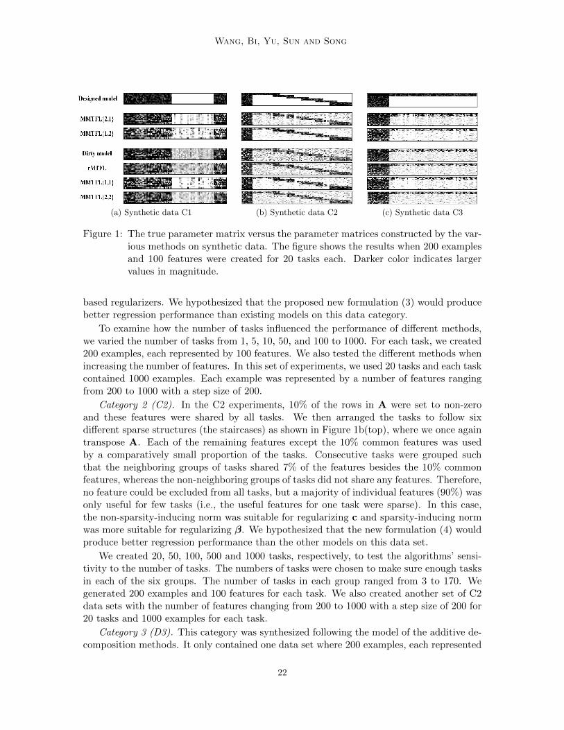
Figure 1: The true parameter matrix versus the parameter matrices constructed by the var-ious methods on synthetic data. The figure shows the results when 200 examplesand 100 features were created for 20 tasks each. Darker color indicates largervalues in magnitude.

based regularizers. We hypothesized that the proposed new formulation (3) would producebetter regression performance than existing models on this data category.

To examine how the number of tasks influenced the performance of different methods,we varied the number of tasks from 1, 5, 10, 50, and 100 to 1000. For each task, we created200 examples, each represented by 100 features. We also tested the different methods whenincreasing the number of features. In this set of experiments, we used 20 tasks and each taskcontained 1000 examples. Each example was represented by a number of features rangingfrom 200 to 1000 with a step size of 200.

Category 2 (C2). In the C2 experiments, 10% of the rows in A were set to non-zeroand these features were shared by all tasks. We then arranged the tasks to follow sixdifferent sparse structures (the staircases) as shown in Figure 1b(top), where we once againtranspose A. Each of the remaining features except the 10% common features was usedby a comparatively small proportion of the tasks. Consecutive tasks were grouped suchthat the neighboring groups of tasks shared 7% of the features besides the 10% commonfeatures, whereas the non-neighboring groups of tasks did not share any features. Therefore,no feature could be excluded from all tasks, but a majority of individual features (90%) wasonly useful for few tasks (i.e., the useful features for one task were sparse). In this case,the non-sparsity-inducing norm was suitable for regularizing c and sparsity-inducing normwas more suitable for regularizing β. We hypothesized that the new formulation (4) wouldproduce better regression performance than the other models on this data set.

We created 20, 50, 100, 500 and 1000 tasks, respectively, to test the algorithms’ sensi-tivity to the number of tasks. The numbers of tasks were chosen to make sure enough tasksin each of the six groups. The number of tasks in each group ranged from 3 to 170. Wegenerated 200 examples and 100 features for each task. We also created another set of C2data sets with the number of features changing from 200 to 1000 with a step size of 200 for20 tasks and 1000 examples for each task.

Category 3 (D3). This category was synthesized following the model of the additive de-composition methods. It only contained one data set where 200 examples, each represented

22


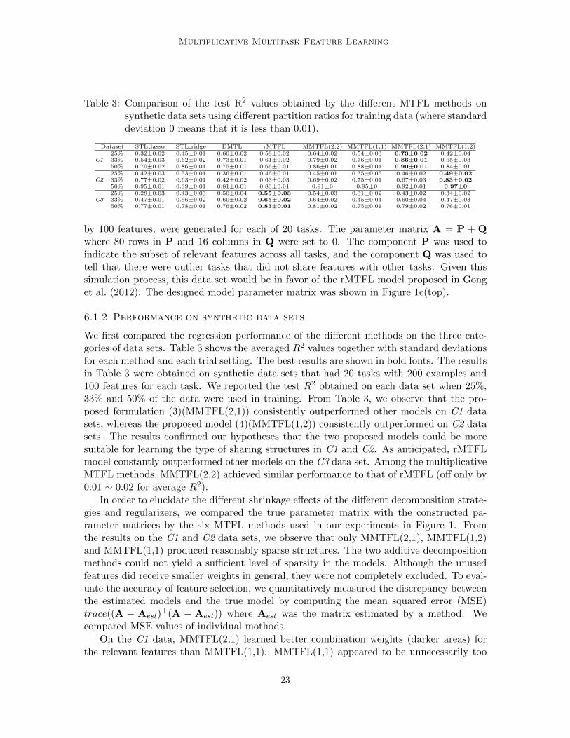
Table 3: Comparison of the test R2 values obtained by the different MTFL methods onsynthetic data sets using different partition ratios for training data (where standarddeviation 0 means that it is less than 0.01).

Dataset STL lasso STL ridge DMTL rMTFL MMTFL(2,2) MMTFL(1,1) MMTFL(2,1) MMTFL(1,2)25% 0.32±0.02 0.45±0.01 0.60±0.02 0.58±0.02 0.64±0.02 0.54±0.03 0.73±0.02 0.42±0.04

C1 33% 0.54±0.03 0.62±0.02 0.73±0.01 0.61±0.02 0.79±0.02 0.76±0.01 0.86±0.01 0.65±0.0350% 0.70±0.02 0.86±0.01 0.75±0.01 0.66±0.01 0.86±0.01 0.88±0.01 0.90±0.01 0.84±0.0125% 0.42±0.03 0.33±0.01 0.36±0.01 0.46±0.01 0.45±0.01 0.35±0.05 0.46±0.02 0.49±0.02

C2 33% 0.77±0.02 0.63±0.01 0.42±0.02 0.63±0.03 0.69±0.02 0.75±0.01 0.67±0.03 0.83±0.0250% 0.95±0.01 0.89±0.01 0.81±0.01 0.83±0.01 0.91±0 0.95±0 0.92±0.01 0.97±025% 0.28±0.03 0.43±0.03 0.50±0.04 0.55±0.03 0.54±0.03 0.31±0.02 0.43±0.02 0.34±0.02

C3 33% 0.47±0.01 0.56±0.02 0.60±0.02 0.65±0.02 0.64±0.02 0.45±0.04 0.60±0.04 0.47±0.0350% 0.77±0.01 0.78±0.01 0.76±0.02 0.83±0.01 0.81±0.02 0.75±0.01 0.79±0.02 0.76±0.01

by 100 features, were generated for each of 20 tasks. The parameter matrix A = P + Qwhere 80 rows in P and 16 columns in Q were set to 0. The component P was used toindicate the subset of relevant features across all tasks, and the component Q was used totell that there were outlier tasks that did not share features with other tasks. Given thissimulation process, this data set would be in favor of the rMTFL model proposed in Gonget al. (2012). The designed model parameter matrix was shown in Figure 1c(top).

6.1.2 Performance on synthetic data sets

We first compared the regression performance of the different methods on the three cate-gories of data sets. Table 3 shows the averaged R2 values together with standard deviationsfor each method and each trial setting. The best results are shown in bold fonts. The resultsin Table 3 were obtained on synthetic data sets that had 20 tasks with 200 examples and100 features for each task. We reported the test R2 obtained on each data set when 25%,33% and 50% of the data were used in training. From Table 3, we observe that the pro-posed formulation (3)(MMTFL(2,1)) consistently outperformed other models on C1 datasets, whereas the proposed model (4)(MMTFL(1,2)) consistently outperformed on C2 datasets. The results confirmed our hypotheses that the two proposed models could be moresuitable for learning the type of sharing structures in C1 and C2. As anticipated, rMTFLmodel constantly outperformed other models on the C3 data set. Among the multiplicativeMTFL methods, MMTFL(2,2) achieved similar performance to that of rMTFL (off only by0.01 ∼ 0.02 for average R2).

In order to elucidate the different shrinkage effects of the different decomposition strate-gies and regularizers, we compared the true parameter matrix with the constructed pa-rameter matrices by the six MTFL methods used in our experiments in Figure 1. Fromthe results on the C1 and C2 data sets, we observe that only MMTFL(2,1), MMTFL(1,2)and MMTFL(1,1) produced reasonably sparse structures. The two additive decompositionmethods could not yield a sufficient level of sparsity in the models. Although the unusedfeatures did receive smaller weights in general, they were not completely excluded. To eval-uate the accuracy of feature selection, we quantitatively measured the discrepancy betweenthe estimated models and the true model by computing the mean squared error (MSE)trace((A − Aest)

>(A − Aest)) where Aest was the matrix estimated by a method. Wecompared MSE values of individual mothods.

On the C1 data, MMTFL(2,1) learned better combination weights (darker areas) forthe relevant features than MMTFL(1,1). MMTFL(1,1) appeared to be unnecessarily too

23


(a) On C1 data (b) On C2 data

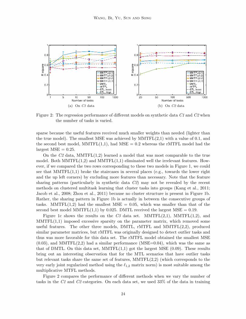
Figure 2: The regression performance of different models on synthetic data C1 and C2 whenthe number of tasks is varied.

sparse because the useful features received much smaller weights than needed (lighter thanthe true model). The smallest MSE was achieved by MMTFL(2,1) with a value of 0.1, andthe second best model, MMTFL(1,1), had MSE = 0.2 whereas the rMTFL model had thelargest MSE = 0.25.

On the C2 data, MMTFL(1,2) learned a model that was most comparable to the truemodel. Both MMTFL(1,2) and MMTFL(1,1) eliminated well the irrelevant features. How-ever, if we compared the two rows corresponding to these two models in Figure 1, we couldsee that MMTFL(1,1) broke the staircases in several places (e.g., towards the lower rightand the up left corners) by excluding more features than necessary. Note that the featuresharing patterns (particularly in synthetic data C2) may not be revealed by the recentmethods on clustered multitask learning that cluster tasks into groups (Kang et al., 2011;Jacob et al., 2008; Zhou et al., 2011) because no cluster structure is present in Figure 1b.Rather, the sharing pattern in Figure 1b is actually in between the consecutive groups oftasks. MMTFL(1,2) had the smallest MSE = 0.05, which was smaller than that of thesecond best model MMTFL(1,1) by 0.025. DMTL received the largest MSE = 0.19.

Figure 1c shows the results on the C3 data set. MMTFL(2,1), MMTFL(1,2), andMMTFL(1,1) imposed excessive sparsity on the parameter matrix, which removed someuseful features. The other three models, DMTL, rMTFL and MMTFL(2,2), producedsimilar parameter matrices, but rMTFL was originally designed to detect outlier tasks andthus was more favorable for this data set. The rMTFL model obtained the smallest MSE(0.03), and MMTFL(2,2) had a similar performance (MSE=0.04), which was the same asthat of DMTL. On this data set, MMTFL(1,1) got the largest MSE (0.09). These resultsbring out an interesting observation that for the MTL scenarios that have outlier tasksbut relevant tasks share the same set of features, MMTFL(2,2) (which corresponds to thevery early joint regularized method using the `1,2 matrix norm) is most suitable among themultiplicative MTFL methods.

Figure 2 compares the performance of different methods when we vary the number oftasks in the C1 and C2 categories. On each data set, we used 33% of the data in training

24


(a) On C1 data (b) On C2 data

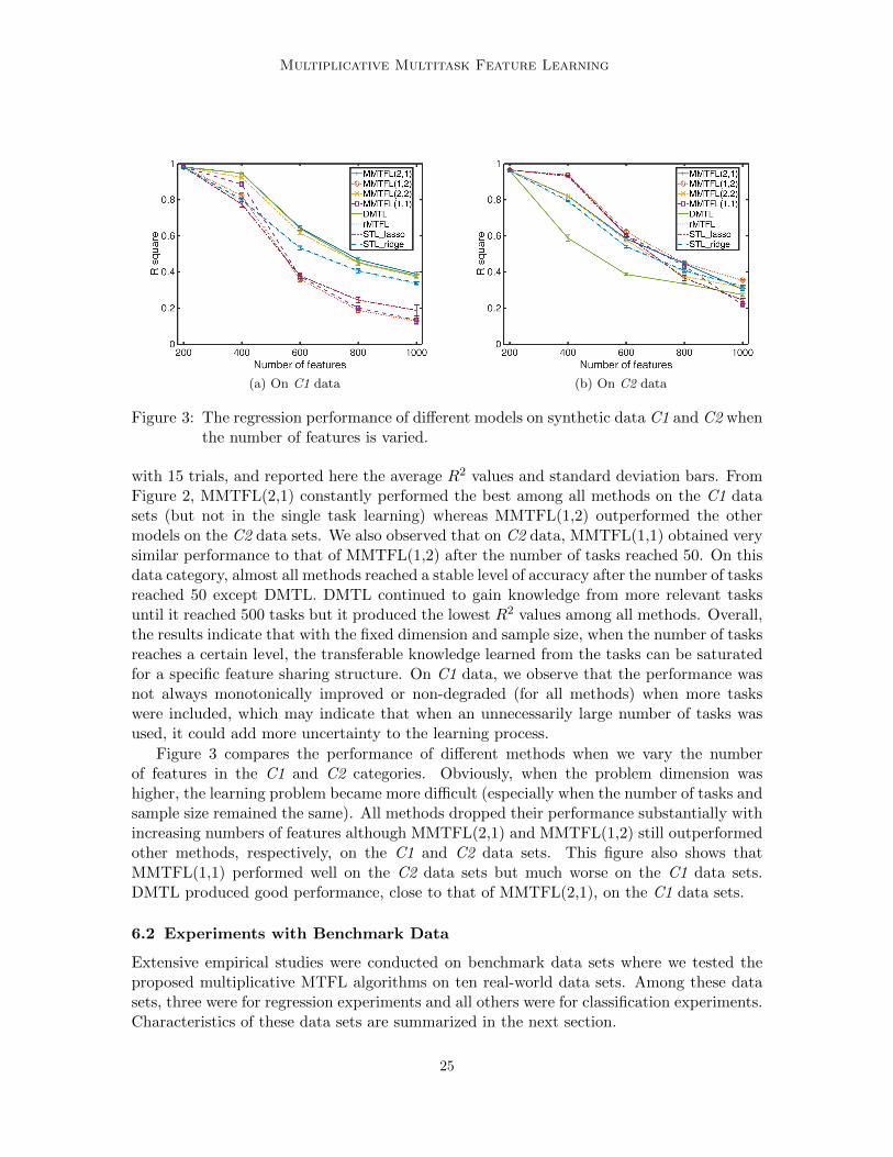
Figure 3: The regression performance of different models on synthetic data C1 and C2 whenthe number of features is varied.

with 15 trials, and reported here the average R2 values and standard deviation bars. FromFigure 2, MMTFL(2,1) constantly performed the best among all methods on the C1 datasets (but not in the single task learning) whereas MMTFL(1,2) outperformed the othermodels on the C2 data sets. We also observed that on C2 data, MMTFL(1,1) obtained verysimilar performance to that of MMTFL(1,2) after the number of tasks reached 50. On thisdata category, almost all methods reached a stable level of accuracy after the number of tasksreached 50 except DMTL. DMTL continued to gain knowledge from more relevant tasksuntil it reached 500 tasks but it produced the lowest R2 values among all methods. Overall,the results indicate that with the fixed dimension and sample size, when the number of tasksreaches a certain level, the transferable knowledge learned from the tasks can be saturatedfor a specific feature sharing structure. On C1 data, we observe that the performance wasnot always monotonically improved or non-degraded (for all methods) when more taskswere included, which may indicate that when an unnecessarily large number of tasks wasused, it could add more uncertainty to the learning process.

Figure 3 compares the performance of different methods when we vary the numberof features in the C1 and C2 categories. Obviously, when the problem dimension washigher, the learning problem became more difficult (especially when the number of tasks andsample size remained the same). All methods dropped their performance substantially withincreasing numbers of features although MMTFL(2,1) and MMTFL(1,2) still outperformedother methods, respectively, on the C1 and C2 data sets. This figure also shows thatMMTFL(1,1) performed well on the C2 data sets but much worse on the C1 data sets.DMTL produced good performance, close to that of MMTFL(2,1), on the C1 data sets.

6.2 Experiments with Benchmark Data

Extensive empirical studies were conducted on benchmark data sets where we tested theproposed multiplicative MTFL algorithms on ten real-world data sets. Among these datasets, three were for regression experiments and all others were for classification experiments.Characteristics of these data sets are summarized in the next section.

25


6.2.1 Benchmark Datasets

Sarcos (Argyriou et al., 2007): Sarcos data were collected for a robotics problem of learningthe inverse dynamics of a 7 degrees-of-freedom SARCOS anthropomorphic robot arm. Eachobservation has 21 features corresponding to 7 joint positions and their velocities and accel-erations. We needed to map from the 21-dimensional input space to 7 joint torques, whichcorresponded to 7 tasks. For each task, we randomly selected 2000 cases for training and theremaining 5291 cases for test. Readers can consult with http://www.gaussianprocess.org/gpml/data/ for more details.

CollegeDrinking (Bi et al., 2013): The college drinking data were collected in orderto identify alcohol use patterns of college students and the risk factors associated withthe binge drinking. The data set contained daily responses from 100 college students toa survey questionnaire measuring various daily measures, such as drinking expectation,negative affects, and level of stress, every day in a 30 day period. The goal was to predictthe amount of nighttime drinks based on 51 daily measures for each student, correspondingto 100 regression tasks. Because there were only 30 records for each person, we used 66%,75% and 80% of the records to form the training set, and the rest for test.

QSAR (Ma et al., 2015): The quantitative structure-activity relationship (QSAR) meth-ods are commonly used to predict biological activities of chemical compounds in the fieldof drug discovery. The data sets we used were collected from three different types of drugactivities, including binding to cannabinoid receptor 1 (CB1), inhibition of dipeptidyl pepti-dase 4 (DPP4) and time dependent 3A4 inhibitions (TDI). For each activity, there were 200molecule examples represented by 2618 features. Three regression models were constructedto simultaneously predict the targets −log(IC50)) of the CB1, DPP4 and TDI effectivenessbased on the molecular features.

C.M.S.C. (Lucas et al., 2013): The Climate Model Simulation Crashes (C.M.S.C.) dataset contained records of simulated crashes encountered during climate model uncertaintyquantification ensembles. The data set comprised 3 tasks. There were 180 examples foreach task. Each example was represented by an 18-dimensional feature vector. Each task isformed by a binary classification problem, which was to predict simulation outcomes (eitherfail or succeed) from the input parameter values for a climate model.

Landmine (Xue et al., 2007): The original Landmine data contained 29 data sets wheresets 1-15 corresponded to the geographical regions that were highly foliated and sets 16-29corresponded to the regions with bare earth or desert. Each data set could be used tobuild a binary classifier. We used the data sets 1-10 and 16-25 to form 20 tasks whereeach example was represented by 9 features extracted from radar images. The number ofexamples varied between individual tasks ranging from 445 to 690.

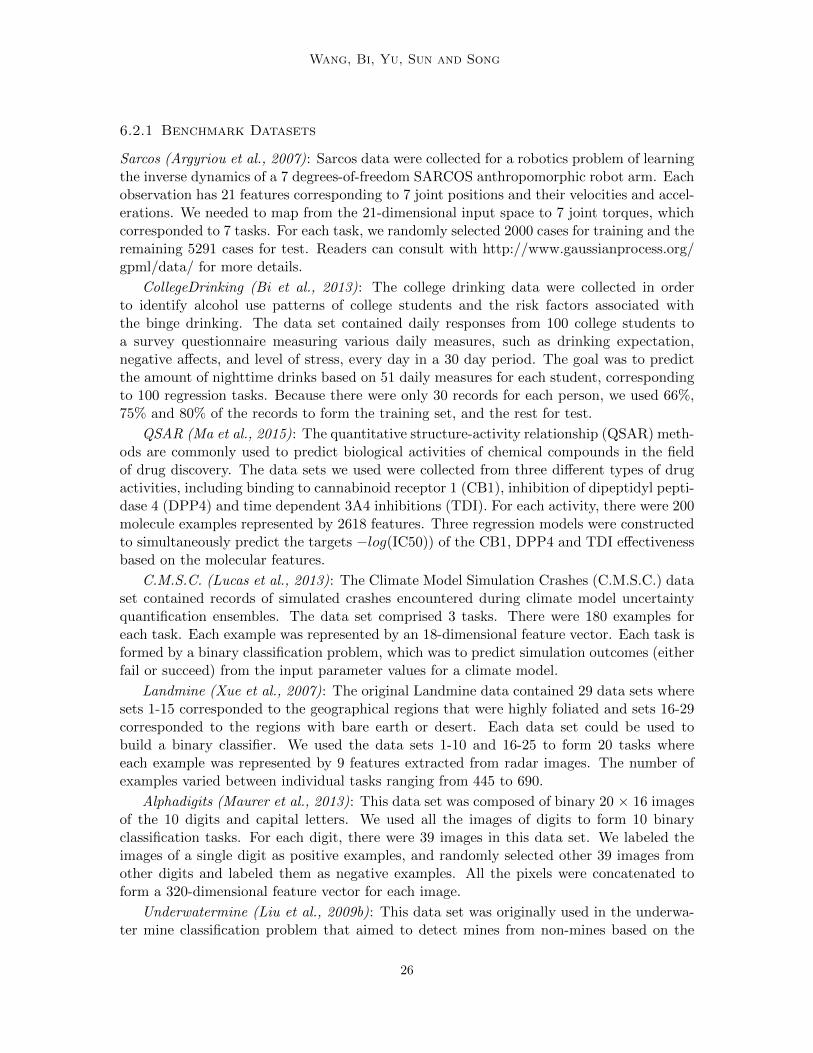
Alphadigits (Maurer et al., 2013): This data set was composed of binary 20 × 16 imagesof the 10 digits and capital letters. We used all the images of digits to form 10 binaryclassification tasks. For each digit, there were 39 images in this data set. We labeled theimages of a single digit as positive examples, and randomly selected other 39 images fromother digits and labeled them as negative examples. All the pixels were concatenated toform a 320-dimensional feature vector for each image.

Underwatermine (Liu et al., 2009b): This data set was originally used in the underwa-ter mine classification problem that aimed to detect mines from non-mines based on the

26


synthetic-aperture sonar images. The data set consisted of 8 tasks with sample sizes rangingfrom 756 to 3562 for each task, and each task was a binary classification problem. Eachexample was represented by 13 features.

Animal recognition (Kang et al., 2011): This data set consisted of images from 20animal classes. Each image was originally represented by 2000 features extracted usingthe bag of word descriptors from the Scale-invariant Feature Transform (SIFT), and thenthe dimensionality was reduced to 202 by a principal component analysis, retaining 95%of the data variance. For each animal class, there were 100 images. We formed 20 binaryclassification tasks where for each task, 100 positive examples were from a specific animalclass and 100 negative examples were randomly sampled from other classes.

HWMA base and HWMA peak (Qazi et al., 2007; Bi and Wang, 2015): The heartwall motion abnormality (HWMA) detection data set was used to analyze and predictif a heart had abnormal motion based on the image features extracted from stress testechocardiographs of 220 patients. The images were taken at the base dose and also peakdose of stress contrast. The wall of left ventricle was medically segmented into 16 segments,and 25 features were extracted from each segment. Every segment of every heart case wasannotated by radiologists in terms of normal or abnormal motions. Thus, there were 16binary classification tasks, each corresponding to one of the 16 heart segments, and eachtask comprised 220 examples.

6.2.2 Performance on real world data sets

Three real-world data sets, the Sarcos, CollegeDrinking and QSAR, were used in regressionexperiments. The performance of the different methods is summarized in Table 4 depictingthe R2 values averaged over the 15 re-partitions in each trial. MMTFL(2,1) achieved thebest R2 values on the Sarcos data set (in all of the 3 trials) and the CollegeDrinkingdata set (in 2 of the 3 trials). The Sarcos data appeared to be in favor of denser modelsgiven MMTFL(2,2) also performed reasonably well on this data set. MMTFL(1,2) modelsachieved the best performance on the QSAR data set consistently across all the 3 trialsettings. On this data set, it was obvious that MMTFL(1,2) was more suitable, whichindicated that most of the 2618 features were useful for some tasks, but the tasks sharedfew features between each other. The difference between the proposed models and theadditively decomposed models ranged from 1 % to 10%, and most importantly, the trendwas consistent for the proposed models to outperform on these data sets.

The other seven real-world data sets were used in classification experiments. Table 5summarizes the results where the F1 scores were averaged across the 15 random splits in eachtrial together with standard derivations. MMTFL(2,1) models achieved consistently thebest performance on the C.S.M.C. and Landmine data sets in comparison with other models.In particular, we observed both MMTFL(1,1) and the MMTFL(2,1) models produced thebest F1 scores in the trial with 33% training split whereas MMTFL(2,1) outperformed allother models in the trial with other partition ratios. These two data sets may prefer across-task sparse models, indicating that many irrelevant features may exist in the data. For theremaining five data sets used in classification experiments, MMTFL(1,2) models showedgenerally better performance than all other models. The difference between the best modeland other MMTFL models could reach 4% to 8%.

27


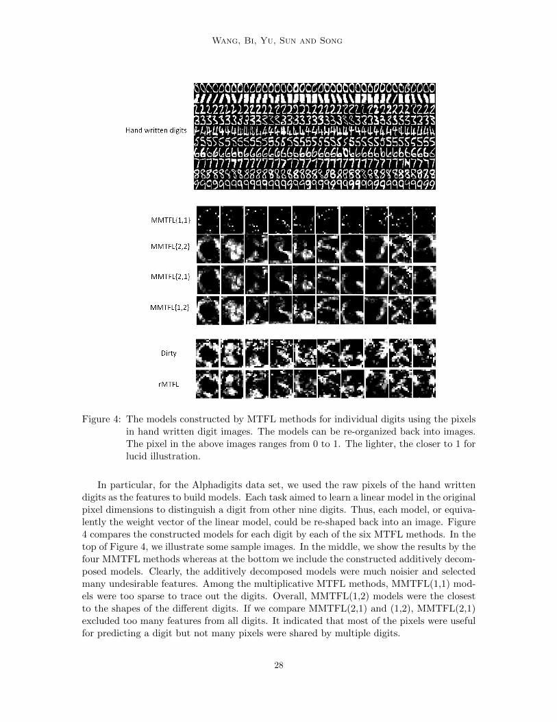
Figure 4: The models constructed by MTFL methods for individual digits using the pixelsin hand written digit images. The models can be re-organized back into images.The pixel in the above images ranges from 0 to 1. The lighter, the closer to 1 forlucid illustration.

In particular, for the Alphadigits data set, we used the raw pixels of the hand writtendigits as the features to build models. Each task aimed to learn a linear model in the originalpixel dimensions to distinguish a digit from other nine digits. Thus, each model, or equiva-lently the weight vector of the linear model, could be re-shaped back into an image. Figure4 compares the constructed models for each digit by each of the six MTFL methods. In thetop of Figure 4, we illustrate some sample images. In the middle, we show the results by thefour MMTFL methods whereas at the bottom we include the constructed additively decom-posed models. Clearly, the additively decomposed models were much noisier and selectedmany undesirable features. Among the multiplicative MTFL methods, MMTFL(1,1) mod-els were too sparse to trace out the digits. Overall, MMTFL(1,2) models were the closestto the shapes of the different digits. If we compare MMTFL(2,1) and (1,2), MMTFL(2,1)excluded too many features from all digits. It indicated that most of the pixels were usefulfor predicting a digit but not many pixels were shared by multiple digits.

28


Tab

le4:

Com

par

ison

ofth

eR

2va

lues

ofth

ed

iffer

ent

MT

FL

met

hod

son

the

ben

chm

ark

regr

essi

on

data

sets

.D

ata

set

ST

Lla

sso

ST

Lri

dge

DM

TL

rMT

FL

MM

TF

L(2

,2)

MM

TF

L(1

,1)

MM

TF

L(2

,1)

MM

TF

L(1

,2)

25%

0.7

5±

0.0

20.7

8±

0.0

20.8

6±

00.8

6±

00.8

9±

00.8

8±

00.8

9±

0.0

10.8

6±

0.0

1S

AR

CO

S33%

0.7

8±

0.0

10.7

8±

0.0

20.8

1±

0.1

10.8

1±

0.1

0.9

0±

00.8

9±

00.9

0±

0.0

10.8

2±

0.0

150%

0.8

2±

0.0

10.8

3±

0.0

60.8

7±

0.1

0.8

7±

0.1

0.8

9±

00.9

0±

0.0

10.9

1±

0.0

10.8

6±

0.0

166%

0.1

5±

0.0

50.0

9±

0.0

20.1

1±

0.0

70.2

2±

0.0

20.2

3±

0.0

40.1

5±

0.0

20.2

1±

0.0

10.1

9±

0.0

4C

oll

egeD

rin

kin

g75%

0.1

8±

0.0

50.1

5±

0.0

20.1

8±

0.0

80.1

8±

0.0

50.1

4±

0.0

50.2

5±

0.0

80.2

7±

0.0

50.2

1±

0.0

880%

0.1

1±

0.0

60.0

9±

0.0

40.1

9±

0.0

60.1

6±

0.0

60.1

9±

0.0

50.1

5±

0.0

40.2

1±

0.0

40.1

5±

0.0

425%

0.3

9±

0.0

30.3

6±

0.0

10.3

9±

0.0

10.3

9±

0.0

10.3

4±

0.0

20.3

8±

0.0

30.3

8±

0.0

30.4

0±

0.0

3Q

SA

R33%

0.3

9±

0.0

40.3

9±

0.0

40.4

0±

0.0

40.3

9±

0.0

40.3

7±

0.0

40.4

1±

0.0

40.4

0±

0.0

50.4

3±

0.0

350%

0.4

4±

0.0

60.4

1±

0.0

30.4

4±

0.0

30.4

4±

0.0

40.4

0±

0.0

60.4

4±

0.0

40.4

5±

0.0

50.4

8±

0.0

4

Tab

le5:

Com

par

ison

ofth

eF

1sc

ores

ofth

ed

iffer

ent

MT

FL

met

hod

son

the

ben

chm

ark

clas

sifi

cati

on

data

sets

.D

ata

set

ST

Lla

sso

ST

Lri

dge

DM

TL

rMT

FL

MM

TF

L(2

,2)

MM

TF

L(1

,1)

MM

TF

L(2

,1)

MM

TF

L(1

,2)

25%

0.3

0±

0.0

40.3

1±

0.0

30.3

6±

00.2

6±

0.0

10.4

0±

00.3

9±

0.0

10.4

3±

00.3

9±

0C

.S.M

.C.

33%

0.3

7±

0.0

20.3

7±

0.0

60.3

7±

0.0

10.3

9±

0.0

10.4

0±

0.0

10.4

5±

0.0

10.4

5±

0.0

10.3

9±

0.0

150%

0.4

0±

0.0

20.4

6±

0.0

10.3

7±

0.0

10.4

4±

0.0

10.4

8±

0.0

10.4

6±

0.0

10.4

9±

0.0

10.4

6±

025%

0.1

4±

0.0

10.0

6±

0.0

10.0

4±

0.0

10.0

6±

00.1±

0.0

10.1

7±

0.0

10.1

7±

0.0

10.1

7±

0.0

1L

an

dm

ine

33%

0.1

3±

0.0

10.1

5±

0.0

10.1

6±

0.0

10.1

6±

0.0

10.1±

0.0

10.1

8±

0.0

10.1

8±

0.0

10.1

2±

0.0

150%

0.1

5±

0.0

10.1

5±

0.0

10.1

8±

0.0

10.2

1±

0.0

10.1

1±

0.0

10.1

9±

0.0

10.2

3±

0.0

10.1

5±

0.0

125%

0.8

6±

0.0

10.7

7±

0.0

10.8

6±

0.0

10.8

6±

00.8

5±

0.0

10.8

4±

0.0

10.7

8±

0.0

10.8

8±

0.0

1A

lph

ad

igit

s33%

0.9

0±

0.0

10.8

7±

0.0

10.9

0±

0.0

10.9

0±

0.0

10.8

7±

0.0

10.8

5±

0.0

10.8

1±

0.0

10.9

1±

0.0

150%

0.9

0±

0.0

10.8

7±

0.0

10.9

1±

0.0

10.9

2±

0.0

10.9

1±

0.0

10.9

0±

0.0

10.8

5±

0.0

10.9

3±

0.0

125%

0.2

4±

0.0

10.2

7±

0.0

20.2

1±

0.0

10.2

7±

00.2

9±

0.0

10.2

4±

0.0

10.2

5±

0.0

10.2

7±

0.0

1U

nd

erw

ate

rm

ine

33%

0.2

5±

0.0

10.3

1±

0.0

20.3

1±

0.0

10.2

9±

0.0

10.3±

0.0

10.3±

0.0

10.2

7±

0.0

10.3

2±

0.0

150%

0.2

7±

0.0

10.2

8±

0.0

10.3

2±

0.0

10.3

4±

0.0

10.3

2±

0.0

10.3

4±

0.0

10.3

5±

0.0

10.3

7±

0.0

125%

0.6

3±

0.0

10.6

3±

0.0

10.6

5±

0.0

10.6

5±

00.6

6±

0.0

10.6

4±

0.0

10.6

3±

0.0

10.6

6±

0.0

1A

nim

al

33%

0.6

6±

0.0

10.6

7±

0.0

10.6

6±

0.0

10.6

5±

0.0

10.6

7±

0.0

10.6

6±

0.0

10.6

6±

0.0

10.6

8±

0.0

150%

0.6

7±

00.6

8±

0.0

10.6

8±

0.0

10.6

6±

0.0

10.6

9±

0.0

10.6

7±

0.0

10.6

8±

0.0

10.6

9±

0.0

125%

0.3

5±

0.0

10.3

7±

0.0

10.4

2±

0.0

10.4±

00.4

6±

0.0

10.3

6±

0.0

10.4

4±

0.0

10.4

5±

0.0

1H

WM

Ab

ase

33%

0.3

8±

0.0

10.3

4±

00.4

5±

0.0

10.4

7±

0.0

1046±

0.0

10.4

4±

0.0

10.4

7±

0.0

10.4

9±

0.0

150%

0.4

4±

0.0

10.4

5±

0.0

10.4

8±

0.0

10.4

8±

0.0

10.5

1±

0.0

10.4

7±

0.0

10.4

7±

0.0

10.5

5±

0.0

125%

0.4

1±

00.4

8±

0.0

10.4

7±

0.0

10.4

7±

00.5

3±

0.0

10.5

3±

0.0

10.5

1±

0.0

10.5

4±

0.0

1H

WM

Ap

eak

33%

0.4

2±

0.0

10.4

7±

0.0

10.4

7±

0.0

10.5±

0.0

10.5

6±

0.0

10.5

5±

0.0

10.5

2±

0.0

10.5

3±

0.0

150%

0.4

4±

0.0

20.5

0±

0.0

20.4

9±

0.0

10.5

1±

0.0

10.5

6±

0.0

10.5

6±

0.0

10.5

5±

0.0

10.5

8±

0.0

1

29


7. Conclusion

In this paper, we have studied a general framework of multiplicative multitask feature learn-ing. By decomposing the model parameter of each task into a product of two components:the across-task feature indicator and task-specific parameters, and applying different regu-larizers to the two components, we can select features for individual tasks and also searchfor the shared features among tasks. We have examined the theoretical properties of thisframework when different regularizers are applied and found that this family of methodscreates models equivalent to those of the joint regularized multitask learning methods butwith a more general form of regularization. Further, we show that this family consists ofsome convex and some non-convex formulations and specify the conditions to obtain con-vexity. An analytical formula is derived for the across-task component as related to thetask-specific component, which sheds light on the different shrinkage effects in the variousregularizers. An efficient algorithm is derived to solve the entire family of methods and alsotested in our experiments for some chosen parameter values. Empirical results on syntheticdata clearly show that there may not be a particular choice of regularizers that is univer-sally better than other choices. We empirically show a few feature sharing patterns thatare in favor of the two newly-proposed choices of regularizers. The extensive experimentalresults on real-world benchmark data sets also confirm the observation and demonstratethe advantages of the proposed two formulations over several existing methods.

Acknowledgments

This work was supported by NSF grants IIS-1320586, DBI-1356655 and the NIH grantR01DA037349. Jinbo Bi was also supported by NSF grants CCF-1514357, IIS-1407205 andIIS-1447711. Correspondence should be addressed to Jinbo Bi ([email protected]).

References

Rie Kubota Ando and Tong Zhang. A framework for learning predictive structures frommultiple tasks and unlabeled data. Journal of Machine Learning Research, 6:1817–1853,December 2005.

Andreas Argyriou, Theodoros Evgeniou, and Massimiliano Pontil. Multi-task feature learn-ing. In Advances in Neural Information Processing Systems, pages 41–48. 2007.

Jinbo Bi and Xin Wang. Learning classifiers from dual annotation ambiguity via a minmaxframework. Neurocomputing, 151, Part 2(0):891 – 904, 2015.

Jinbo Bi, Tao Xiong, Shipeng Yu, Murat Dundar, and R. Bharat Rao. An improved multi-task learning approach with applications in medical diagnosis. In Proceedings of the 2008European Conference on Machine Learning and Knowledge Discovery in Databases - PartI, pages 117–132, 2008.

Jinbo Bi, Jiangwen Sun, Yu Wu, Howard Tennen, and Stephen Armeli. A machine learningapproach to college drinking prediction and risk factor identification. ACM Transactionson Intelligent Systems Technology, 4:72:1–72:24, 2013.

30


Edwin Bonilla, Kian Ming Chai, and Christopher Williams. Multi-task gaussian processprediction. In Advances in neural information processing systems, pages 153–160, 2007.

Jianhui Chen, Jiayu Zhou, and Jieping Ye. Integrating low-rank and group-sparse struc-tures for robust multi-task learning. In Proceedings of ACM International Conference onKnowledge Discovery and Data Mining (SIGKDD), pages 42–50, 2011.

Theodoros Evgeniou and Massimiliano Pontil. Regularized multi–task learning. In Pro-ceedings of ACM International Conference on Knowledge Discovery and Data Mining(SIGKDD), pages 109–117, 2004.

Pinghua Gong, Jieping Ye, and Changshui Zhang. Robust multi-task feature learning. InProceedings of ACM International Conference on Knowledge Discovery and Data Mining(SIGKDD), pages 895–903, 2012.

Pinghua Gong, Jieping Ye, and Changshui Zhang. Multi-stage multi-task feature learning.The Journal of Machine Learning Research, 14(1):2979–3010, 2013.

Irwin R Goodman and Samuel Kotz. Multivariate θ-generalized normal distributions. Jour-nal of Multivariate Analysis, 3(2):204–219, 1973.

William H. Greene. Econometric Analysis. Prentice Hall, fifth edition, 2002.

Shengbo Guo, Onno Zoeter, and Cedric Archambeau. Sparse bayesian multi-task learning.In Advances in Neural Information Processing Systems, pages 1755–1763, 2011.

Laurent Jacob, Bach Francis, and Jean-Philippe Vert. Clustered multi-task learning: aconvex formulation. In Advances in Neural Information Processing Systems, pages 745–752, 2008.

Ali Jalali, Sujay Sanghavi, Chao Ruan, and Pradeep K Ravikumar. A dirty model formulti-task learning. In Advances in Neural Information Processing Systems, pages 964–972, 2010.

Zhuoliang Kang, Kristen Grauman, and Fei Sha. Learning with whom to share in multi-taskfeature learning. In Proceedings of the International Conference on Machine Learning,pages 521–528, 2011.

Abhishek Kumar and Hal Daume III. Learning task grouping and overlap in multi-tasklearning. In Proceedings of the International Conference on Machine Learning, pages1383–1390, 2012.

Seunghak Lee, Jun Zhu, and Eric Xing. Adaptive multi-task lasso: with application toeQTL detection. In Advances in Neural Information Processing Systems, pages 1306–1314. 2010.

Su-In Lee, Vassil Chatalbashev, David Vickrey, and Daphne Koller. Learning a meta-level prior for feature relevance from multiple related tasks. In Proceedings of the 24thInternational Conference on Machine Learning, pages 489–496, New York, NY, USA,2007.

31


Jun Liu, Shuiwang Ji, and Jieping Ye. Multi-task feature learning via efficient `1,2-normminimization. In Proceedings of the Conference on Uncertainty in Artificial Intelligence,pages 339–348, 2009a.

Qiuhua Liu, Xuejun Liao, Hui Li, Jason R Stack, and Lawrence Carin. Semisupervisedmultitask learning. Pattern Analysis and Machine Intelligence, IEEE Transactions on,31(6):1074–1086, 2009b.

Aurelie Lozano and Grzegorz Swirszcz. Multi-level lasso for sparse multi-task regression. InProceedings of the International Conference on Machine Learning, pages 361–368, 2012.

D. D. Lucas, R. Klein, J. Tannahill, D. Ivanova, S. Brandon, D. Domyancic, and Y. Zhang.Failure analysis of parameter-induced simulation crashes in climate models. GeoscientificModel Development Discussions, 6(1):585–623, 2013.

Junshui Ma, Robert P. Sheridan, Andy Liaw, George E. Dahl, and Vladimir Svetnik. Deepneural nets as a method for quantitative structureactivity relationships. Journal of Chem-ical Information and Modeling, 55(2):263–274, 2015.

Andreas Maurer, Massimiliano Pontil, and Bernardino Romera-Paredes. Sparse coding formultitask and transfer learning. In Proceedings of the 30th International Conference onMachine Learning, pages 343–351, 2013.

L. Meier, S. v. d. Geer, and P. Buhlmann. The group lasso for logistic regression. Journalof the Royal Statistical Society: Series B, 70 Part 1:53–71, 2008.

Charles A Micchelli, Jean M Morales, and Massimiliano Pontil. Regularizers for structuredsparsity. Advances in Computational Mathematics, 38(3):455–489, 2013.

Guillaume Obozinski and Ben Taskar. Multi-task feature selection. In Technical report,Statistics Department, UC Berkeley, 2006.

Alexandre Passos, Piyush Rai, Jacques Wainer, and Hal Daume III. Flexible modeling oflatent task structures in multitask learning. In Proceedings of the International Conferenceon Machine Learning, pages 1103–1110, 2012.

M. Qazi, G. Fung, S. Krishnan, J. Bi, B. Rao, and A. Katz. Automated heart abnormalitydetection using sparse linear classifiers. IEEE Engineering in Medicine and Biology, 26(2):56–63, 2007.

Ariadna Quattoni, Xavier Carreras, Michael Collins, and Trevor Darrell. An efficient pro-jection for l1,infinity regularization. In Proceedings of the International Conference onMachine Learning, pages 108–115, 2009.

Piyush Rai and Hal Daume. Infinite predictor subspace models for multitask learning. InInternational Conference on Artificial Intelligence and Statistics, pages 613–620, 2010.

P. Tseng. Convergence of a block coordinate descent method for nondifferentiable mini-mization. Journal of Optimization Theory and Applications, 109(3):475–494, 2001.

32


B. A. Turlach, W. N. Wenables, and S. J. Wright. Simultaneous variable selection. Tech-nometrics, 47(3):349–363, 2005.

T. Xiong, J. Bi, B. Rao, and V. Cherkassky. Probabilistic joint feature selection for multi-task learning. In Proceedings of SIAM International Conference on Data Mining, pages69–76, 2006.

Y. Xue, X. Liao, L. Carin, and B. Krishnapuram. Multi-task learning for classification withdirichlet process priors. Journal of Machine Learning Research, 8:35–63, 2007.

Ming Yang, Yingming Li, and Zhongfei Mark Zhang. Multi-task learning with gaussianmatrix generalized inverse gaussian model. In Proceedings of the 30th International Con-ference on Machine Learning, pages 423–431, 2013.

Kai Yu, Volker Tresp, and Anton Schwaighofer. Learning gaussian processes from multipletasks. In Proceedings of the 22Nd International Conference on Machine Learning, pages1012–1019, New York, NY, USA, 2005.

Shipeng Yu, Volker Tresp, and Kai Yu. Robust multi-task learning with t-processes. InProceedings of the 24th International Conference on Machine Learning, pages 1103–1110,2007.

Yu Zhang and Dit-Yan Yeung. A convex formulation for learning task relationship in multi-task learning. In Proceedings of the Conference on Uncertainty in Artificial Intelligence,pages 733–742, 2010.

Yu Zhang, Dit-Yan Yeung, and Qian Xu. Probabilistic multi-task feature selection. InAdvances in Neural Information Processing Systems, pages 2559–2567, 2010.

Peng Zhao, Guilherme Rocha, and Bin Yu. The composite absolute penalties family forgrouped and hierarchical variable selection. The Annals of Statistics, pages 3468–3497,2009.

Jiayu Zhou, Jianhui Chen, and Jieping Ye. Clustered multi-task learning via alternatingstructure optimization. In Advances in Neural Information Processing Systems, pages702–710, 2011.

Y. Zhou, R. Jin, and S. C.H. Hoi. Exclusive lasso for multi-task feature selection. InProceedings of International Conference on Artificial Intelligence and Statistics, pages988–995, 2010.

33

multiplicative multitask feature learningjinbo/doc/15-234.pdf · multiplicative multitask feature...

Documents