multiprocessor real-time scheduling on general...
TRANSCRIPT

Multiprocessor Real-Time Scheduling on
General Purpose Operating Systems
Bridging the gap between Theory and Practice
Juri Lelli
ReTiS Lab.
Scuola Superiore Sant’Anna
A thesis submitted for the degree of
Doctor of Philosophy
Supervisor: Prof. Giuseppe Lipari
June the XXth, 2014


Abstract
From the perspective of an user the differences between desktop, server and
mobile computing systems are less and less noticeable. They all ship multicore or
multiprocessor CPUs and they all run similar applications on top of a General Pur-
pose Operating Systems (GPOS). Moreover, applications runtime requirements
often fall under the domain of Real-Time systems, for which not only the func-
tional correctness of a computation, but also its timeliness is important. One of
the key roles of a GPOS is then to provide, under a common interface, low-level
mechanisms enabling the development of applications that can meet the needs of
end users. At the same time, such an Operating System has to remain backward
compatible with older platform (e.g., small singleprocessors), while being efficient
throughout the whole spectrum of computing systems. On the other side, real-time
academic literature usually abstracts from these requirements, as is constantly an-
ticipating problems of future generation platforms. Unfortunately, the strong focus
on theoretical aspects induces a gap between the two worlds, where knowledge cre-
ated by the latter is usually hard to be applied to the former, as practical issues
often arise.
This thesis wants to make the gap a bit more shallow, by developing strategies
to enable the use of classical multiprocessor real-time scheduling mechanisms on a
modern GPOS. To this end, we focus on the Linux kernel, as its use is nowadays
widespread on all the aforementioned platforms. We first present a sofware addition
to the Linux scheduler implementing Earliest Deadline First (EDF) and Constant
Bandwidth Server (CBS) algorithms, going by the name of SCHED DEADLINE;
indeed, a major outcome of this work is the inclusion of SCHED DEADLINE in the
mainline version of the Linux kernel. We also detail software solutions that allow
efficient real-time scheduling on a big multiprocessor system, and how the devel-
opment of such solutions was eased by means of a user-space scheduler simulator.
Secondly, building on top of our implementation, we report about a comparison
between two classical real-time scheduling algorithms (Rate Monotonic (RM) and
EDF) in order to help software developers choosing the right algorithm to schedule
real-time tasks. In this part we both consider runtime overheads due to implemen-
tation choices and cache-related delays originating from the presence of memory
hierachies. We finally add to the picture problems that arise when concurrent
i

ii ABSTRACT
real-time tasks share resources, and detail about theoretical extensions and a prac-
tical evaluation of one resource sharing algorithm called Multiprocessor Bandwidth
Inheritance (M-BWI).

To my family and to Grazia,
you guys rock!


Contents
Abstract i
List of Figures vii
List of Tables xi
Introduction 1
Chapter 1. Real-Time Systems 5
1.1. Real-Time Task Model 5
1.2. Hard and Soft Real-Time Requirements 7
1.3. Real-Time Scheduling 7
1.3.1. Uniprocessor Scheduling 8
1.3.2. Multiprocessor Scheduling 9
1.4. Real-Time Operating Systems 9
1.4.1. Predictability Issues 10
1.4.2. Design Opportunities 11
Chapter 2. Real-Time Scheduling on General Purpose Operating Systems 13
2.1. Introduction 13
2.1.1. Contributions 13
2.1.2. The Linux Scheduler 14
2.2. SCHED DEADLINE 15
2.2.1. Implementation Details 16
2.2.2. User-level API 18
2.2.3. Experiments 18
2.2.4. Data Structures for Efficient Global Scheduling 26
2.2.5. Idle processor improvement 26
2.2.6. Heap Data structure 27
2.2.7. Evaluation 29
2.3. PRAcTISE 34
2.3.1. Developing Kernel-level code in User-Space 34
2.3.2. State Of Art 35
2.3.3. Architecture 37
2.3.4. Ready queues 37
v

vi CONTENTS
2.3.5. Locking and synchronisation 38
2.3.6. Event generation and processing 38
2.3.7. Data structures in PRAcTISE 41
2.3.8. Statistics 42
2.3.9. Evaluation 43
2.4. Conclusions 48
Chapter 3. When Theory comes to Hardware 49
3.1. Setting the Ground 49
3.2. An experimental comparison 52
3.3. State of Art 53
3.4. Experimental Setup 54
3.4.1. Hardware Platform 54
3.4.2. Task Structure 55
3.4.3. Task Set Generation 55
3.4.4. Scheduling and Allocation 56
3.4.5. Performance and Overhead Evaluation 57
3.5. Experimental Results 59
3.5.1. Running Each Task Alone 59
3.5.2. Impact of Scheduling 60
3.5.3. Working Set Size and Cache Behaviour 64
3.5.4. Scheduling Overheads Comparison 66
3.6. Conclusions 67
Chapter 4. Resource Reservation & Shared Resources on SMP 71
4.1. Introduction 71
4.2. State of the art 71
4.2.1. Model of a critical section 71
4.2.2. Admission Control 72
4.2.3. Combining resource reservations and critical sections 73
4.2.4. Interacting tasks 74
4.2.5. The M-BWI protocol 74
4.3. Implementation 75
4.3.1. Priority Inheritance in Linux 76
4.3.2. The implementation of M-BWI 78
4.3.3. Issues with clustered scheduling 81
4.4. Evaluation 83
4.4.1. Experimental setup 83
4.4.2. Runtime validation 83
4.4.3. Overheads measurements 85
4.5. Conclusions 87

CONTENTS vii
Chapter 5. Conclusions 89
5.1. Summary of Results 89
5.2. Future Work 90
Bibliography 93


List of Figures
1.1 Typical parameters of a real-time task. 6
2.1 Linux modular scheduling frameworki (until version 3.13). 14
2.2 Linux modular scheduling framework, since Linux 3.14. 16
2.3 struct dl rq extended 17
2.4 SCHED DEADLINE API 19
2.5 SCHED DEADLINE serving a periodic task and two CPU hungry
(greedy) tasks. 19
2.6 Inter-Frame Times for MPlayer scheduled with different SCHED DEADLINE parameters. 22
2.7 Cumulative Distribution Function of the MPlayer’s Inter-Frame Times
for different values of the SCHED DEADLINE maximum runtime. 23
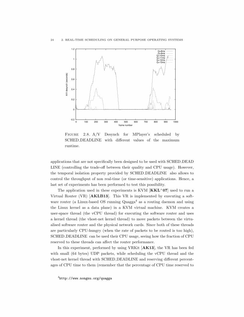
2.8 A/V Desynch for MPlayer’s scheduled by SCHED DEADLINE with
different values of the maximum runtime. 23
2.9 Throughput of a KVM-based virtual router as a function of the
percentage of CPU time reserved to the vCPU thread. 25
2.10 Throughput of a KVM-based virtual router as a function of the
percentage of CPU time reserved to the vhost-net kernel thread. 25
2.11 Find CPU eligible for push. 27
2.12 Using idle CPU mask. 27
2.13 Heap implementation with a simple array. 28
2.14 Heap structure. 28
2.15 Find eligile CPU using a heap. 28
2.16 Architecture of a single processor (Multi Chip Module) of the Dell
PowerEdge R815. 30
2.17 Number of push cycles for average loads of 0.6. 31
2.18 Number of push cycles for average loads of 0.8. 32
2.19 Number of enqueue cycles for average loads of 0.6. 33
2.20 Number of enqueue cycles for average loads of 0.8. 33
2.21 Main scheduling functions in PRAcTISE 40
ix

x LIST OF FIGURES
2.22 Instruction that guarantee serialization. 43
2.23 Comparison using diff. 45
2.24 Number of cycles (mean) to a) modify and b) query the global data
structure (cpudl vs. cpupri), kernel implementation. 46
2.25 Number of cycles (mean) to a) modify and b) query the global data
structure (cpupri), on PRAcTISE. 47
2.26 Number of cycles (mean) to a) modify and b) query the global data
structure (cpudl), on PRAcTISE. 47
2.27 Number of cycles (mean) to a) modify and b) query the global
data structure for speed-up SCHED DEADLINE pull operations, on
PRAcTISE. 48
3.1 Two level memory system. 50
3.2 Three level memory system. 50
3.3 Cache effects on a quad-core machine. 52
3.4 One of the used task-sets with U=0.6 and 96 tasks. 59
3.5 Execution times obtained for the various tasks (averaged over the task
activations) under C-EDF (plus signs) and G-EDF (multiply signs)
relative to the figures obtained under P-EDF, in the cases of 16KB
(top) and 256KB (bottom) WSS. 62
3.6 CDF of the normalised laxity for all the tasks as obtained under various
scheduling policies, with U=0.8 and 96 tasks. 63
3.7 CDF of the normalised laxity for the minimum-period (top) and
maximum-period (bottom) tasks, under various scheduling policies,
with U=0.8 and 96 tasks. 64
3.8 CDF of the obtained normalised laxity for clustered EDF and RM
policies with WSS of 16KB and 256KB, with U=0.8 and 96 tasks. 65
4.1 A task exhaust its budget while in a critical section, thus increasing
the blocking time of another task. 73
4.2 Example of M-BWI: τA, τB , τC , executed on 2 processors, that access
only mutex M1. 75
4.3 Deadline miss caused by a task inheriting bandwidth and deadline but
not affinity from a blocked task. 82
4.4 Deadline miss caused by a task inheriting both bandwidth and affinity
from a blocked task. 82
LIST OF FIGURES xi
4.5 Two task (τ1 and τ3) sharing one resource (protected by a normal
mutex). A third independent task (τ2) arrives and preempts τ3 even if
τ1’s server has higher priority than τ2’s. 84
4.6 Two task (τ1 and τ3) sharing one resource (protected by a M-BWI-
enabled mutex). A third independent task (τ2) has to wait τ1’s server
replenishment event to start executing. 84
4.7 System with two CPUs. Two task (τ1 and τ3) sharing one resource
(protected by a M-BWI-enabled mutex). Other two independent tasks
(τ2 and τ4) are pinned each one on a different CPU. 85
4.8 Kernel functions durations (in µs) from a run on a real machine. 86
4.9 Kernel functions durations (in µs) with nested critical sections, from a
run on a real machine. 87


List of Tables
2.1 Percentage of missed deadline for partitioned scheduling, as a function
of the load U =∑ Ci
Piexpressed as a percentage. 20
2.2 Percentage of missed deadline for global scheduling, as a function of
the load U =∑ Ci
Pi. 21
2.3 Locking and synchronisation mechanisms (Linux vs. PRAcTISE). 39
2.4 Differences between user-space and kernel code. 44
3.1 Algorithms vs. scheduling solutions: possible configurations. 57
3.2 Evaluation metrics. 58
3.3 Cache behaviour with tasks from the task-sets executed in isolation. 60
3.4 Statistics for the metrics of interest when WSS=16KB, under various
configurations: global (top table), clustered (middle table) and
partitioned (bottom table) scheduling, both with EDF and RM
policies. 61
3.5 Cache related behaviour of global (top sub-table), clustered (middle
sub-table) and partitioned (bottom sub-table) EDF and RM policies for
various configurations (values are averages of all the runs for each
configuration) and WSS. 65
3.6 Scheduling and migration related function durations (on average, in
clock cycles) for global (top sub-table), clustered (middle sub-table)
and partitioned (bottom sub-table) EDF and RM policies, in the case of
WSS=16KB. 67
xiii


Introduction
The goal of this thesis is to reduce the gap between real-time literature and
industry, in the context of General Purpose Operating Systems (GPOSes), by devel-
oping real-time scheduling algorithms and verifying their performance on Symmetric
Multiprocessing (SMP) systems.
This work is motivated by the widespread adoption of GPOSes on modern mul-
tiprocessors platforms to perform activities that requires certain degrees of time-
liness (e.g., video processing, audio/video streaming, VoIP, etc.). The GPOS of
reference is Linux, as it is nowadays widely adopted on the whole spectrum of
computing platforms, ranging from small hand-held devices to cloud computing in-
frastructures. Even if Linux is born as a traditional GPOS, in the last years, there
has been a considerable interest in using it also for real-time and control, from
both academy and industry [Edg13]. We believe that this is mainly due to the
free availability of its source code, the support for a great number of architectures
and the existence of countless applications running on it. However, Linux has not
been in origin tought as a Real-Time Operating System (RTOS), thus it lacks of
mechanisms that allow a classical real-time feasibility study of the system under
development; i.e., developers cannot be sure that timing requirements will be met
even correctly knowing the runtime timing behavior of their applications. Indeed,
POSIX-compliant fixed-priority scheduling policies, already offered by Linux, do
not fit real-time users needs, as they are not much sophisticated.
Similarly to our approach, modification to the Linux kernel have been pro-
posed, such as RT-Linux 1, proposed by Yodaiken et al. [YB97], and RTAI 2,
proposed by Dozio et al. [DM03], in order to enable hard real-time computing in a
Linux-like environment. In these solutions, a real-time micro-kernel layer is added
between the real hardware and the Linux OS, which runs as the background/idle
activity whenever there are no hard real-time tasks active in the system. This al-
lows for respecting the very tight timing constraints (microsecond-level) typical of
industrial automation and robotic applications. However, applications that want
1Originally supplied by FSMLabs (http://www.fsmlabs.com/), acquired by Wind
River in 2007 and discontinued in 2011.2https://www.rtai.org
1

2 INTRODUCTION
to use real-time facilities are typically required to be adapted or rewritten. More-
over, we believe that the fact that these solutions remain bounded to the efforts
of some academic entity limit their usage from industry, for which discontinuous
updates to the last Linux version could represent a problem. It must be also noted
the fact that a key feature like the temporal isolation property [BLAC06] is usu-
ally neglected and not implemented in both general purpose and real-time OSes.
In fact, without such mechanism, a high priority task runs undisturbed until it
blocks, indipendently from what considered at analysis/design phase. This can ob-
viously jeopardize guarantees offered to other tasks and activities of the system, till
the point the whole system becomes unusable. With our mechanisms application
developers are guaranteed that the performance that their applications exibit in
isolation (i.e., when run alone on the system) are not affected by other applications
concurrently running on the system (and we give advices on how to cope with cases
when perfect isolation cannot be guaranteed).
Among others, a modification to the Linux kernel purposely targeted for aca-
demic research is the LITMUSRT testbed 3, developed by the Real-Time System
Group at University of North Carolina at Chapel Hill. The primary purpose of the
testbed is to provide a useful experimental platform for applied real-time system
research. Indeed, solutions developed on top of it can serve as a proof of concept
for the engineering of the same solutions on plain Linux, even if a proper implemen-
tation on Linux is usually harder to be realized. As this project is not focused on
industry, there are currently no plans to turn it into a production-quality system.
Moreover, the API (i.e., interface to applications) is not stable and may change
without warning between releases (nor the release schedule is fixed).
We instead targeted the inclusion of our contributions (at least the bigger
part of them) in the mainline (stock) Linux kernel as another goal of this work.
The aim is to transfer back knowledge to the Linux community, from which we
copiously drew both as code base (the Linux kernel itself) and with requests for
advice (through the Linux kernel mailing list). So our intent is different from
LITMUSRT one, as we trade a certain less flexibility on our solutions with strict
adherence to Linux design choices, and we do so because we firmly believe that this
approach could foster a wider usage and understanding of real-time concepts by
industry.
The main contributions of this thesis are:
• an efficient extension of the SCHED DEADLINE patchset for the Linux
scheduler for SMP systems;
• an evalutation of the performance of such a real-time extension for appli-
cations users;
3http://www.litmus-rt.org/

INTRODUCTION 3
• the development of a user-space emulator of the Linux scheduler subsys-
tem on a multi-core architecture and an evaluation of different solution to
speed-up scheduling on such kind of systems;
• an experimental comparison of several configurations of two classical real-
time scheduling algorithms on NUMA machines;
• a proof-of-concept implementation of the Multiprocessor Bandwidth In-
heritance protocol on Linux.
An key outcome of the work performed while doing this thesis has also been
the inclusion in the mainline Linux kernel (since Linux version 3.14) of almost all
the code we built upon our research.
The reminder of this thesis is organized as follows. Chapter 1 discusses needed
notation and background on real-time systems. Chapter 2 provides an overview on
the current status of real-time scheduling mechanisms on General Purpose Oper-
ating Systems, and details about our modifications to one of such GPOSes, Linux.
Moreover, it also discuss how a user-space emulator can ease real-time scheduling
algorithms development on a multi-core platform. Chapter 3 builds upon both the
developed mechanisms and the stock Linux scheduler to perform an experimental
study of applicability of classical real-time theory on Non-Uniform Memory Access
systems. Chapter 4 provides a proof-of-concept solution that allows to perform a
feasiblity analysis of a real-time system using Linux even in presence of task ac-
cessing shared resources. Finally, Chapter 5 concludes with a summary of the work
presented in this thesis and with the discussion of how work could extend the results
presented.


CHAPTER 1
Real-Time Systems
In this chapter we provide a general introduction to real-time systems. No-
tation and definition are given that put the basis for the following chapters. We
also detail about differences and peculiarities of Uniprocessor and Multiprocessors
systems. We conclude the chapter with a taxonomy of different approaches in de-
signing Operating Systems, and the predictability issues that may arise when such
Operating Systems have to provide support for real-time applications.
1.1. Real-Time Task Model
Real-Time systems are computing systems that contain concurrent computa-
tional activities for which, not only correctness of results, but also timeliness is
crucial. These computational activities are called tasks and each task may spawn
a (potentially infinite) sequence of jobs during its lifetime. A job is thus a se-
quential unit of work. Timeliness requirements pertain to tasks and are embodied
by deadlines, which represent the time before which a process should complete its
execution.
We assume (unless otherwise specified, like in Chapter 4) that tasks adhere
to the classical sporadic task model [But11]. The system is comprised of n real-
time tasks τ1, τ2, . . . , τn, that constitute a taskset τ = τ1, τ2, . . . , τn. Each task
generates a sequence of jobs τi,1, τi,2, τi,3, /dots. A job τi,j is characterized by
several parameters:
Release/Arrival time (ri,k): is the instant of time at which the job becomes
ready for execution (since it has been activated by some event or condition).
Computation time (ci,k): is the time necessary to the processor to execute the
job without interruption.
Start time (si,k): is the time at which the job starts its execution for the first
time (i.e., the processor is assigned to τi,k for the first time).
Finishing/Completion time (fi,k): is the time at which the job completes its
execution.
Relative deadline (Di,k): is the interval of time within which the job execution
should complete with respect to its release time. We usually have a single value for
5

6 1. REAL-TIME SYSTEMS
every job of a certain task that is still called relative deadline and it is denoted as
Di (as it refers to task τi).
Absolute deadline (di,k): is the absolute instant of time by which job τi,k should
complete, in order to preserve the timeliness properties of the system. The absolute
deadline is computed based on the relative deadline and the release time: di,k =
ri,k +Di,k.
Response time (Ri,k): is the difference between the finishing time and the release
time: Ri,k = fi,k − ri,k.
Lateness (Li,k): is the delay of a job completion with respect to its deadline:
Li,k = fi,k − di,k. Note that, if the job completes before its deadline, its lateness
is negative. Instead, when a job completes after its deadline, its lateness is posive,
and in this case we say that a deadline miss event occurred.
Tardiness or Exceeding time (Ei,k): is the time a job stays active after its
deadline: Ei,k = max(0, Li,k).
Worst case execution time (Ci): shortened with WCET, is the worst (i.e.,
maximum) computation time of all jobs of task τi: Ci = max(ci,k).
Some of the above parameters are illustrated in Figure 1.1. Usually, new arrivals
are represented with upward arrows and deadlines with downward arrows.
ri,k si,k fi,k di,k
ci,k
Figure 1.1. Typical parameters of a real-time task.
Task Periodicity Another timing characteristic that can be associated to a real-
time task is the regularity of its activations. Commonly, tasks are distinguished
between periodic and aperiodic.
Periodic tasks are activated (released) at regular intervals of time. Specifically,
a task τi is said to be periodic if, for every pair of consecutive jobs, ri,k+1 = ri,k+Ti,
where Ti is the task period. The period is also used to calculate the share of system
processor resource a task uses once it is activated. This parameter is called task
utilization and corresponds to Ui = Ci
Ti. Therefore, a taskset composed by n tasks
will have a total utilization of:
U =
n∑i=1
Ui.
When activations are not strictly periodic (e.g., a task that is activated only
when an aperiodic event occurs), but still there is some bounded separation among
them, tasks are said to be sporadic. In this case, the parameter Ti denotes the

1.3. REAL-TIME SCHEDULING 7
minimum separation between successive jobs of the same task, and is also called
minimum interarrival time. We thus have: ri,k+1 ≥ ri,k + Ti (note the greater or
equal relation between release times). The sporadic task model is a generalization
of the periodic task model.
Lastly, real-time tasks for which no constrain on a certain separation between
consecutive activations can be given are called aperiodic. The only obvious ob-
servation that can be made is that jobs activations still follow a sequence, i.e.
ri,k+1 ≥ ri,k.
1.2. Hard and Soft Real-Time Requirements
As already stated, one characteristic of real-time tasks is that for them timeli-
ness is of key importance : a real-time job should complete (and produce a result)
before its absolute deadline, otherwise the produced result, even if correct, may be
too late to be useful. Depending on the criticality of this timing requirement, we
can split real-time tasks in two classes: hard and soft tasks.
A task τi is a hard real-time (HRT) task if no job deadline must be missed
(i.e., Ei,k = 0). HRT systems are comprised of HRT tasks only. A task τi is a
soft real-time task (SRT) if some missed deadline are allowed for it. Systems that
contain one or more SRT tasks are called soft real-time systems.
Hence, for HRT tasks correctness implies both correct results and no deadline
misses. Instead, for SRT tasks, this notion has no single definition, being the extent
of permissible deadline violations (tardiness) very application-dependent. In this
thesis we adopt the notion of bounded tardiness [DA08] (i.e., each job is allowed
to complete within some bounded amount of time after its deadline). It must be
noted that the HRT correctness is a special case of the SRT bounded tardiness. In
fact, for HRT tasks the relation Ei,k = 0 must always hold.
1.3. Real-Time Scheduling
In an Operating System (OS) kernel, the scheduler is responsible for choosing
which task (also called process or thread) executes on each processor at any given
time. In real-time systems this is done by first assigning priorities to tasks, then a
real-time scheduling algorithm, implemented by the scheduler, uses such priorities
to perform scheduling decisions. Furthermore, priorities can be fixed for the whole
lifetime of a task, or change dynamically, according to some logic or external/in-
ternal event.
Fixed priority scheduling. In fixed priority scheduling, once a priority has been
assigned to a task, it remains the same for the task’s lifetime, and it also corresponds
to the priority of every job of the task. The most popular fixed priority scheme is

8 1. REAL-TIME SYSTEMS
the Rate Monotonic (RM) algorithm, for which each task τi gets a priority pi that
is inversely proportional to its period (pi ∝ 1Ti
).
Dynamic priority scheduling. In dynamic priority scheduling, the priority of a
task can change over time. In this thesis we focus on Job-Level Dynamic Priority
(JLDP) algorithms, for which priority of different jobs of the same task can change,
but once a priority has been assigned to a job, it remains the same till the job com-
pletion. The most widely known JLDP real-time scheduling algorithm is Earliest
Deadline First (EDF), for which the job with the earliest absolute deadline di is
assigned the highest dynamic priority.
Feasibility analysis. A schedule is the assignment (produced by the scheduler) of
all jobs in the system on the available processors. Furthermore, in a valid schedule:
(i) every processor is assigned to at most one job at any time, (ii) every job is
scheduled on at most one processor at any time, and (iii) jobs are not scheduled
before their release time.
A taskset τ is feasible on a given hardware platform if there exists a schedule
(feasible schedule) in which every job of τ meets its deadline. A HRT taskset
τ is said to be (HRT) schedulable on a hardware platform by algorithm A if A
always produces a feasible schedule for τ (i.e., no job of τ misses its deadline under
A). Moreover, A is an optimal scheduling algorithm if A correctly schedules every
feasible task system. Relaxing the correctness notion, a SRT taskset τ is (SRT)
schedulable under the scheduling algorithm A if the maximum tardiness is bounded.
Scheduling algorithms performance are usually compared through the schedu-
lable utilization bound (or simply utilization bound). If Ub(A) is a utilization bound
for the scheduling algorithm A, then A can correctly schedule every task system
with U(τ) ≤ Ub(A). Note that, unless an optimal utilization bound is known for
A (e.g., EDF on UP), the previous condition is only sufficient, but not necessary.
In fact, there may exist a taskset τ with U(τ) > Ub(A) that is schedulable using A
(e.g., RM with few tasks).
1.3.1. Uniprocessor Scheduling
In [LL73], Liu and Layland showed that RM is optimal among fixed-priority
algorithms and they derived an utilization bound for RM for periodic task systems:
Ub = n(21/n−1), that for high values of n tends to Ub = ln 2 ' 0.69. The feasibility
analysis of the RM algorithm can also be performed using a different approach called
Hyperbolic Bound [BBB03]:
n∏i=1
(Ui + 1) ≤ 2.
The test has the same complexity of the original Liu and Layland bound, but it is
less pessimistic.
1.4. REAL-TIME OPERATING SYSTEMS 9
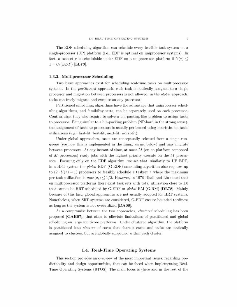
The EDF scheduling algorithm can schedule every feasible task system on a
single-processor (UP) platform (i.e., EDF is optimal on uniprocessor systems). In
fact, a taskset τ is schedulable under EDF on a uniprocessor platform if U(τ) ≤1 = Ub(EDF ) [LL73].
1.3.2. Multiprocessor Scheduling
Two basic approaches exist for scheduling real-time tasks on multiprocessor
systems. In the partitioned approach, each task is statically assigned to a single
processor and migration between processors is not allowed; in the global approach,
tasks can freely migrate and execute on any processor.
Partitioned scheduling algorithms have the advantage that uniprocessor sched-
uling algorithms, and feasibility tests, can be separately used on each processor.
Contrariwise, they also require to solve a bin-packing-like problem to assign tasks
to processor. Being similar to a bin-packing problem (NP-hard in the strong sense),
the assignment of tasks to processors is usually performed using heuristics on tasks
utilizations (e.g., first-fit, best-fit, next-fit, worst-fit).
Under global approaches, tasks are conceptually selected from a single run-
queue (see how this is implemented in the Linux kernel below) and may migrate
between processors. At any instant of time, at most M (on an platform composed
of M processors) ready jobs with the highest priority execute on the M proces-
sors. Focusing only on the EDF algorithm, we see that, similarly to UP EDF,
in a HRT system the global EDF (G-EDF) scheduling algorithm also requires up
to (2 · U(τ) − 1) processors to feasibly schedule a taskset τ where the maximum
per-task utilization is max(ui) ≤ 1/2. However, in 1978 Dhall and Liu noted that
on multiprocessor platforms there exist task sets with total utilization close to 1.0
that cannot be HRT scheduled by G-EDF or global RM (G-RM) [DL78]. Mainly
because of this fact, global approaches are not usually adopted for HRT systems.
Nonetheless, when SRT systems are considered, G-EDF ensure bounded tardiness
as long as the system is not overutilized [DA08].
As a compromise between the two approaches, clustered scheduling has been
proposed [CAB07], that aims to alleviate limitations of partitioned and global
scheduling on large multicore platforms. Under clustered algorithm, the platform
is partitioned into clusters of cores that share a cache and tasks are statically
assigned to clusters, but are globally scheduled within each cluster.
1.4. Real-Time Operating Systems
This section provides an overview of the most important issues, regarding pre-
dictability and design opportunities, that can be faced when implementing Real-
Time Operating Systems (RTOS). The main focus is (here and in the rest of the

10 1. REAL-TIME SYSTEMS
thesis) on Linux-based RTOS, as Linux is nowadays largely used by both academia
and industry to perform activities that fall in the real-time domain.
1.4.1. Predictability Issues
Linux has been designed as a General Purpose Operating Systems, so it is no
wonder that it can experiment problems with HRT. In particular, the main issues
of predictability under Linux are due to:
• Non-preemptable critical sections. Several execution paths in the kernel
cannot be preempted and interrupts are disabled during the execution
of certain IRQ managements routines. These factors can cause priority
inversions and thus unpredictability for real-time activities.
• Non-predictable duration of IRQ management routines. Even though
Linux adopts a split-interrupt management schema, the duration of IRQ
managements routines is non predictable and can thus affect predictability
of the system.
• Throughput oriented scheduling. Linux has been designed to be through-
put oriented. Scheduling decisions on multiprocessor systems tend to
evenly distribute the load among available processors, without consider-
ing priorities or any effect related to the presence of caches and memories.
This may cause unneeded migrations, high overhead and tasks execution
time variance, impacting system predictability.
In order to solve these problems (in what follows we will explicitly deal with
the last point) several approaches to modify Linux has been proposed, that can be
divided into mono- and dual-kernel variants.
Mono-kernel approach
Under this approach, high predictability is achieved addressing the aforemen-
tioned limitation with modification of the Linux kernel. This approach is in common
between some commercial RTOSs (e.g., MontaVista Linux 1, timesys 2, etc.) and
by the open-source PREEMPT RT patch for the Linux kernel 3. This patch allows
nearly all of the kernel to be preempted, with the exception of a few small region
of code. This is achieved by replacing most kernel spinlocks (a simple single-holder
lock) with mutexes that support priority inheritance, as well as moving all interrupts
and software interrupts to kernel threads. It has to be noted that our contributions
are orthogonal to this first approach (user of the last version of the PREEMPT RT
patch, based on Linux version 3.14, can find our contributions already included)
and can actually address point three above (whereas PREEMPT RT solves point
one and two).
1http://www.mvista.com/solution-real-time.html2http://www.timesys.com/3https://rt.wiki.kernel.org/index.php/CONFIG PREEMPT RT Patch

1.4. REAL-TIME OPERATING SYSTEMS 11
Dual-kernel approach
Under this approach, a virtualization layer is employed to concurrently execute
two (or more) operating systems on the same hardware. Although this additional
layer may introduce additional overhead and latencies, this second approach allows
to isolate GPOSs like Linux for RTOSs, thus avoiding the predictability issues
detailed above. Linux-derived RTOSs like RTAI 4 and RTLinux 5 employ a dual-
kernel approach to meet the requirements of HRT tasks. Dual-kernel approaches
are also employed by commercial RTOSs like VxWorks 6.
1.4.2. Design Opportunities
Free availability of the Linux kernel source code gives the impression that the
desing space for modifications of its internal meachanisms is boundless. And this
is almost true, unless one doesn’t plan to propose such modifications to the Linux
kernel development community. The community is responsible, through the work
of subsystems maintainers, for guaranteeing that Linux remains efficient on a vast
set of hardware platform. This is accomplished via a thorough review process of
patches proposed to the community, and, understandably, big changes and complete
rewrites of core subsystems are generally frowned upon. The Linux scheduler makes
no exception; being one of the most important subsystems, it is actually very
refractory to modifications.
The main design characteristic that constrain design space for new modifica-
tions are:
• Low overhead. The scheduler must be extremely fast in deciding which
process to run next. No heavy operations are thus allowed. Purpose built
data structures are usually employed to speed up scheduling decisions.
• Seamless integration in the scheduler framework. The Linux scheduler
has a modular design (see Section 2.1.2. New scheduling policies must fit
in this desing.
• Distributed design. As we will describe in more details in Section 2.1.2,
the Linux scheduler performs scheduling decision in a distributed manner.
In particular, each CPU has its own runqueue and global scheduling is
achieved through tasks migrations among runqueues. There is flexibility
in deciding how migration decisions happen.
• Fast acceptance/refusal of new tasks entering the system. The scheduler
is also responsible for deciding if a new task can enter the system (e.g., if
the user has enough permissions for choosing a scheduling policy). Such
4https://www.rtai.org5Originally supplied by FSMLabs (http://www.fsmlabs.com/), acquired by Wind
River in 2007 and discontinued in 2011.6http://www.windriver.com/products/vxworks/index.html

12 1. REAL-TIME SYSTEMS
decisions must be quickly perfomed. A heavy machinery, even if more
accurate, is usually not allowed.
We decided to adhere to these constraints as we planned inclusion of our mod-
ifications in the mainline Linux kernel right from the beginning.

CHAPTER 2
Real-Time Scheduling on General Purpose
Operating Systems
2.1. Introduction
In this and in the following chapter, we argue that real-time scheduling is
indeed possible also on top of General Purpose Operating Systems (GPOS). We
will focus on the Linux kernel, given its widespread adoption and the availability
of its source code, but the obtained results can be generalized to other GPOS
having the same structure of Linux and running on top of nowadays multi-core
and multiprocessor machines. We specifically address issues detailed in Section 1.4
giving an overview of the design choices we made considering the design constraints
of Section 1.4.2. Furthermore, we keep our focus close to the point of view of an
application developer. In effect, we advise the use of the following technologies
as a way to improve efficiency and predictability of a vast number of classes of
applications.
2.1.1. Contributions
In this chapter, we first present the implementation of a global EDF sched-
uler in Linux, called SCHED DEADLINE [FCTS09]. We also show how we optimized
global scheduling on SMP systems using a heap data structure. After describing the
base real-time scheduler of Linux (Section 2.1.2), and our implementation (Section
2.2), we compare its performance against the global POSIX-compliant fixed pri-
ority scheduler of Linux and with a previous version of SCHED DEADLINE (Section
2.2.7). The results show that using appropriate data structures it is in-
deed possible to build efficient and scalable global real-time schedulers.
SCHED DEADLINE is part of the mainline Linux kernel since version 3.14.
We then propose PRAcTISE (PeRformance Analysis and TestIng of real-time
multicore SchEdulers) for the Linux kernel: it is a framework for developing,
testing and debugging scheduling algorithms in user space before imple-
menting them in the Linux kernel. In addition, PRAcTISE allows to compare
different implementations by providing early estimations of their relative perfor-
mance. In this way, the most appropriate data structures and scheduler structure
can be chosen and evaluated in user-space. Compared to other similar tools, like
13

14 2. REAL-TIME SCHEDULING ON GENERAL PURPOSE OPERATING SYSTEMS
LinSched, the proposed framework allows true parallelism thus permitting a
full test in a realistic scenario.
2.1.2. The Linux Scheduler
Since release 2.6.23, the Linux scheduler is implemented as a modular frame-
work that can be easily extended. The current structure has been implemented by
Ingo Molnar as a replacement of the previous O(1) scheduler. The structure consists
of a core block, providing basic funtionalities, and a set of scheduling classes, each
encapsulating one or more specific scheduling policy. Scheduling policies determine
when and how tasks are selected to run. Figure 2.1 shows the set of scheduling
policies traditionally available in Linux (i.e., until version 3.13).
Figure 2.1. Linux modular scheduling frameworki (until version 3.13).
Each scheduling policy of Figure 2.1 belongs to one of the two scheduling
classes Linux had before version 3.13. First scheduling class, implemented in
kernel/sched/fair.c, is intended for fair scheduling of non-real-time activities
(SCHED NORMAL, SCHED BATCH and SCHED IDLE policies). Second scheduling class
is providing fixed priority real-time scheduling (SCHED FIFO or SCHED RR policies),
following the POSIX 1001.3b [IEE04] specification and is implemented in kernel
/sched/rt.c. For what concern tasks priorities, scheduling classes are stacked
upon each other, where lower classes have also lower priorities. As it is indicated in
the picture, real-time scheduling policies have higher priority than fair scheduling
policies, i.e., tasks belonging to the latter are always preempted by tasks sched-
uled by the former. In this thesis we will focus specifically on real-time scheduling
policies.
2.1. INTRODUCTION 15
Run-queues, masks and locks
To keep track of active tasks, the scheduler uses a data structure called run-
queue. There is one runqueue for each CPU and they are managed separately in
a distributed manner. Every runqueue is protected by a spin-lock to guarantee
correctness on concurrent updates. Runqueues are modular, in the sense that there
is a separate sub-runqueue for each scheduling class. Tasks are enqueued on some
runqueue when they wake up and are dequeued when they are suspended.
Key components of the fixed priority sub-runqueue are:
• a priority array on which tasks are actually queued;
• fields used for load balancing;
• fields to speed up decisions on a multiprocessor environment.
The fixed priority scheduling class already supports global scheduling. Tasks are
migrated across CPUs (runqueues) following an active load balancing approach that
is realized through push and pull operations, see below.
An additional data structure, called cpupri, is used to reduce the amount of
work needed for a push operation. This structure tracks the priority of the highest
priority task in each runqueue. The system maintains the state of each CPU with
a 2 dimensional bitmap: the first dimension is for priority class and the second for
CPUs in that class. Therefore a push operation can find a suitable CPU where to
send a task in O(1) time, since it has to perform a two bits search only (if we don’t
consider affinity restriction).
Push and pull operations
When a task is activated on CPU k, first the scheduler checks the local run-
queue to see if the task has higher priority than the executing one. In this case, a
preemption happens, and the preempted task is inserted at the head of the queue;
otherwise the waken-up task is inserted in the proper runqueue, depending on the
state of the system. In case the head of the queue is modified, a push operation is
executed to see if some task can be moved to another queue. When a task suspends
itself (due to blocking or sleeping) or lowers its priority on CPU k, the scheduler
performs a pull operation: it looks at the other run-queues to see if some other
higher priority tasks need to be migrated to the current CPU. Pushing or pulling a
task entails modifying the state of the source and destination runqueues: the sched-
uler has to dequeue the task from the source and then enqueue it on the destination
runqueues.

16 2. REAL-TIME SCHEDULING ON GENERAL PURPOSE OPERATING SYSTEMS
2.2. SCHED DEADLINE
At the time of writing, a new scheduling class/policy has been merged in the
Linux kernel, called SCHED DEADLINE [FCTS09]. It implements partitioned, clus-
tered and global EDF scheduling with hard and soft reservations 1. SCHED DEADLINE
is seamless integrated in the Linux scheduler modular framework. The scheduling
policy is implemented in kernel/sched/deadline.c and extends the set of tradi-
tionally available scheduling policies as can be seen in Figure 2.2.
Figure 2.2. Linux modular scheduling framework, since Linux 3.14.
In this section 2, we describe the implementation of SCHED DEADLINE and
we evaluate its properties running synthetic benchmarks and real applications on a
Linux systems. We then detail about a heap data structure we designed and devel-
oped to optimize access to the earliest deadline tasks (the implementation is now
part of SCHED DEADLINE [FCTS09]). After describing the base real-time scheduler
of Linux (Section 2.1.2), and our implementation (Section 2.2), we compare its per-
formance against the global POSIX-compliant fixed priority scheduler of Linux and
with a previous version of SCHED DEADLINE (Section 2.2.7). The results show that
using appropriate data structures it is indeed possible to build efficient
and scalable global real-time schedulers.
The code developed during the experimental evaluation phase of this part can
be downloaded by following the instructions on this page: http://retis.sssup.
it/~jlelli/sched-deadline.php.
1Full source code merged in mainline since Linux 3.14.2Claudio Scordino contributed to Section 2.2.2 and Luca Abeni performed experi-
ments of Sections 2.2.3, the content of these Sections has been submitted for publication.

2.2. SCHED DEADLINE 17
struct dl_rq {
struct rb_root rb_root;
struct rb_node *rb_leftmost;
unsigned long dl_nr_running;
#ifdef CONFIG_SMP
struct {
/* two earliest tasks in queue */
u64 curr;
u64 next; /* next earliest */
} earliest_dl;
int overloaded;
unsigned long dl_nr_migratory;
unsigned long dl_nr_total;
struct rb_root pushable_tasks_root;
struct rb_node *pushable_tasks_leftmost;
#endif /* CONFIG_SMP */
};
Figure 2.3. struct dl rq extended
2.2.1. Implementation Details
The approach used for the implementation is the same used in the Linux ker-
nel for the fixed-priority scheduler. This is usually called distributed run-queue,
meaning that each CPU maintains a private data structure implementing its own
ready queue and, if global scheduling is to be achieved, tasks are migrated among
processors when needed.
In more details:
• the tasks of each CPU are kept into a CPU-specific run-queue, imple-
mented as a red-black tree ordered by absolute deadlines;
• tasks are migrated among run-queues of different CPUs for the purpose
of fulfilling the following constraints:
– on m CPUs, the m earliest deadline ready tasks run;
– the CPU affinity settings of all the tasks is respected.
Migration points are the same as in the fixed priority scheduling class. Decisions
related to push and pull logic are taken considering deadlines (instead of priorities)
and according to tasks affinity and system topology. The data structure used to
represent the EDF ready queue of each processor has been modified, as shown in
Figure 2.3 (new fields are the one inside the #ifdef CONFIG SMP block).

18 2. REAL-TIME SCHEDULING ON GENERAL PURPOSE OPERATING SYSTEMS
• earliest dl is a per-runqueue data structure used for “caching” the dead-
lines of the first two ready tasks, so to facilitate migration-related deci-
sions;
• dl nr migratory and dl nr total represent the number of queued tasks
that can migrate and the total number of queued tasks, respectively;
• overloaded serves as a flag, and it is set when the queue contains more
than one task;
• pushable tasks root is the root of the red-black tree of tasks that can
be migrated, since they are queued but not running, and it is ordered by
increasing deadline;
• pushable tasks leftmost is a pointer to the node of pushable tasks root
containing the task with the earliest deadline.
A push operation tries to move the first ready and not running task of an
overloaded queue to a CPU where it can execute. The best CPU where to push
a task is the one which is running the task with the latest deadline among the m
executing tasks, considering also the constraints due to the CPU affinity settings.
A pull operation tries to move the most urgent ready and not running tasks among
all tasks on all overloaded queues in the current CPU.
2.2.2. User-level API
The existing system calls sched setscheduler() and sched getscheduler()
have not been extended, due to the binary compatibility issues that modifying the
sched param data structure would have raised for existing applications. Therefore,
two new system calls called sched setattr() and sched getattr() have been
introduced. These syscalls also support the other existing scheduling policies —
i.e., the interpretation of the arguments depends on the selected policy. Therefore,
they are expected to replace the previous system calls (which will be left to not
break existing applications). The prototype of these new system calls is shown in
Figure 2.4.
2.2.3. Experiments
Greedy tasks
As a first experiment, we have used SCHED DEADLINE to schedule one peri-
odic task (that executes for 1ms every 4ms) and two greedy tasks (tasks which never
blocks, and try to consume all the CPU time) scheduled by two CBSs (1ms, 6ms)
and (1ms, 10ms). Figure 2.5 shows a segment of the schedule. As periodic task
is the one with most strict timing requirements (relative deadline is 4ms) it gets
always scheduled when it wakes up. Greedy 1 is also higher priority than Greedy 2,
and it preempts the latter during the first activation (remember that priorities are
dynamic, the behavior is thus relative to this particular timing window). Another
thing to notice is that greedy tasks are throttled once they try to execute for more

2.2. SCHED DEADLINE 19
#include <sched.h>
struct sched_attr {
u32 size;
u32 sched_policy;
u64 sched_flags;
/* SCHED_OTHER , SCHED_BATCH */
s32 sched_nice;
/* SCHED_FIFO , SCHED_RR */
u32 sched_priority;
/* SCHED_DEADLINE */
u64 sched_runtime;
u64 sched_deadline;
u64 sched_period;
};
int sched_setattr(pid_t pid ,
const struct sched_attr *attr);
int sched_getattr(pid_t pid ,
const struct sched_attr *attr ,
unsigned int size);
Figure 2.4. SCHED DEADLINE API
than the allowed budget (red lines in the figure), while the periodic task always
goes to sleep before exausting its budget, and it is never throttled.
This experiment shows that SCHED DEADLINE is capable of creating an
effective isolation between the running tasks, so that greedy, buggy or misbehaving
tasks cannot affect the execution of the other running tasks.
Synthetic Real-Time Workloads
In order to show how SCHED DEADLINE allows to properly schedule real-time
applications, some sets of periodic real-time tasks have been randomly generated
with taskgen [ESD10] and executed by a user-level application (named rt-app)
either under the SCHED DEADLINE or the SCHED OTHER (i.e., CFS) scheduling

20 2. REAL-TIME SCHEDULING ON GENERAL PURPOSE OPERATING SYSTEMS
Figure 2.5. SCHED DEADLINE serving a periodic task and two
CPU hungry (greedy) tasks.
Table 2.1. Percentage of missed deadline for partitioned schedul-
ing, as a function of the load U =∑ Ci
Piexpressed as a percentage.
U(%) SCHED DEADLINE SCHED OTHER
60% 0% 0.58%
70% 0% 0.9%
80% 0% 2.61%
90% 0% 5.88%
policies. When using SCHED DEADLINE , each task τi has been assigned a run-
time Qi slightly larger than its execution time Ci, and a server period Ti equal to
the task period Pi.
This experiment has been performed considering both partitioned scheduling
and global scheduling. In the partitioned scheduling case, tasks were statically
bound to a CPU core (using the Linux cpuset mechanism), and the load on each
core increased from 0.6 (60%) to 0.9 (90%). Notice that the U = 1 case (100% CPU
utilization) has been avoided in order to leave some spare time for the other tasks
running in the system, so that the OS is not starved by SCHED DEADLINE tasks.
For each CPU load, 50 tasksets were randomly generated.
Table 2.1 shows the percentage of missed deadlines when using SCHED DEADLINE or
CFS to schedule the tasksets. As it can be noticed from the table, SCHED DEADLINE is
able to avoid any missed deadline (because the load on each core is smaller than
1, and because the CBS parameters have been assigned in order to exploit the so-
called hard schedulability property of the CBS). On the other hand, CFS performs
pretty well, but is not able to avoid missing deadlines.
After testing partitioned scheduling, the experiment has been repeated by con-
figuring SCHED DEADLINE to do global EDF scheduling. In this case, the Linux
cpuset mechanism is not used and tasks are able to migrate between all of the
available CPU cores. Since these experiments have been performed using 4 of the
6 cores provided by the Xeon CPU, the tasksets have been generated with a total

2.2. SCHED DEADLINE 21
Table 2.2. Percentage of missed deadline for global scheduling,
as a function of the load U =∑ Ci
Pi.
U(%) SCHED DEADLINE SCHED OTHER
340% 0.77% 3.75%
350% 0.78% 6.17%
360% 1.29% 6.92%
370% 1.69% 8.52%
380% 2.38% 10.62%
390% 3.54% 14.15%
utilization ranging from U = 3.4 (340%) to U = 3.9 (390%). Again, the U = 4 case
has not been considered in order to avoid starving the system. As for the previous
experiment, 50 taskset per CPU load have been randomly generated.
Table 2.2 shows the percentage of missed deadlines when using SCHED DEAD
LINE or CFS to schedule the tasksets: in case of global scheduling, EDF is not able
to guarantee that no deadline will be missed, so SCHED DEADLINE experiences
some missed deadlines. The standard CFS scheduler, however, exhibits a percentage
of missed deadlines that is more than 4 times the percentage experienced by the
CBS.
These sets of experiments show two things:
• On uni-processor systems or when the tasksets can be statically parti-
tioned between multiple CPUs / CPU cores, SCHED DEADLINE is suit-
able to schedule hard real-time tasks (no missed deadlines);
• On multi-processor (or multi-core) systems where the taskset cannot be
statically partitioned between CPUs / cores and global scheduling must be
used, SCHED DEADLINE allows to reduce the number of missed dead-
lines (respect to other CPU schedulers) improving the performance of soft
real-time tasks.
SCHED DEADLINE on a Real Application
After showing how SCHED DEADLINE helps in respecting the timing con-
straints of real-time tasks using some randomly generated synthetic workloads, the
effectiveness of the new scheduling policy is now shown on a real application. In
particular, we have performed a set of tests using MPlayer3, a simple yet widely
used and powerful video player. Being single-threaded, it can be easily scheduled
through a single reservation.
3http://www.mplayerhq.hu

22 2. REAL-TIME SCHEDULING ON GENERAL PURPOSE OPERATING SYSTEMS
MPlayer has been modified to measure some important quality of service met-
rics when reproducing a video: the Inter-Frame Time (IFT) — defined as the
difference between the display time of the current and the previous frame — and
the Audio / Video desynchronisation (A/V Desynch) — defined as the difference
between the Presentation TimeStamp (PTS) of the currently reproduced audio
sample and the PTS of the currently reproduced video frame. Variations in the
IFT can have a bad impact of the perceived video quality, because the video does
not play smoothly, while large values of the A/V Desynch affect the quality of
the reproduced media because audio and video do not appear synchronised (think
about lip synch).
0
10000
20000
30000
40000
50000
60000
70000
80000
90000
0 100 200 300 400 500 600
Inte
r-F
ram
e T
ime
(u
s)
Frame Number
Q = 7ms
0
10000
20000
30000
40000
50000
60000
70000
80000
0 100 200 300 400 500 600
Inte
r-F
ram
e T
ime
(u
s)
Frame Number
Q = 10ms
Figure 2.6. Inter-Frame Times for MPlayer scheduled with dif-
ferent SCHED DEADLINE parameters.
MPlayer has then been used to play a HD movie (with H.264 video and AAC+
audio), and scheduled by using SCHED DEADLINE with a period equal to the ex-
pected IFT (1 / fps) and a runtime (maximum budged) ranging from 5ms to 20ms.
Since the video frame rate is 23.976fps, the expected IFT is 1000000/23.976 =
41708µs. As expected, if the runtime was large enough, the IFT was stable around
the expected value of 41708µs. Decreasing the maximum budged, some jitter
started to be visible in the IFT. Finally, for small values of Qi, the IFT was out
of control. Figure 2.6 shows the IFT measured for the first 600 frames with a
value of the maximum runtime near to the one needed to decode without issues
(Qi = 10ms) and a smaller value, which created issues and a non fluid playback
(Qi = 7ms).

2.2. SCHED DEADLINE 23
0
0.1
0.2
0.3
0.4
0.5
0.6
0.7
0.8
0.9
1
0 20000 40000 60000 80000 100000 120000 140000
CD
F
Inter-Frame Time (us)
Q=5msQ=7ms
Q=10msQ=13ms
Figure 2.7. Cumulative Distribution Function of the
MPlayer’s Inter-Frame Times for different values of the
SCHED DEADLINE maximum runtime.
Figure 2.7 shows the impact of different Qi values on the IFTs by plotting
their Cumulative Distribution Function (CDF). Notice how increasing Qi allows
to make the CDF more similar to a step function (indicating that MPlayer has
a probability near to 1 to play the video always at the correct rate), at the cost
of dedicating more CPU time to MPlayer’s execution. This experiment shows how
SCHED DEADLINE allows to respect the temporal constraints of real applications
(and not only synthetic benchmarks), and to find proper trade-offs between QoS
and CPU usage.
Finally, Figure 2.8 displays the A/V Desynch experienced for different values
of Qi, showing again how SCHED DEADLINE can be used to control the qual-
ity perceived by a user and to guarantee the proper behaviour of time-sensitive
applications.
Summing up, SCHED DEADLINE provides a good amount of control over the
real-time performance of real applications, because it allows to better specify the
applications’ parameters and requirements: since the user can communicate to the
scheduler some temporal constraints to be respected (in the form of a period Ti
and a runtime Qi), the scheduler can do a better work in trying to respect these
constraints.
Using SCHED DEADLINE to Control the Application Throughput
The previous experiments showed how SCHED DEADLINE allows to respect
the deadlines of real-time applications and to properly serve “legacy” time-sensitive
24 2. REAL-TIME SCHEDULING ON GENERAL PURPOSE OPERATING SYSTEMS
-0.2
0
0.2
0.4
0.6
0.8
1
1.2
0 100 200 300 400 500 600 700 800 900 1000
A/V
de
syn
ch (
seco
nd
s)
frame number
Q=8msQ=9ms
Q=10msQ=11msQ=12msQ=13ms
Figure 2.8. A/V Desynch for MPlayer’s scheduled by
SCHED DEADLINE with different values of the maximum
runtime.
applications that are not specifically been designed to be used with SCHED DEAD
LINE (controlling the trade-off between their quality and CPU usage). However,
the temporal isolation property provided by SCHED DEADLINE also allows to
control the throughput of non real-time (or time-sensitive) applications. Hence, a
last set of experiments has been performed to test this possibility.
The application used in these experiments is KVM [KKL+07] used to run a
Virtual Router (VR) [AKLB13]. This VR is implemented by executing a soft-
ware router (a Linux-based OS running Quagga4 as a routing daemon and using
the Linux kernel as a data plane) in a KVM virtual machine. KVM creates a
user-space thread (the vCPU thread) for executing the software router and uses
a kernel thread (the vhost-net kernel thread) to move packets between the virtu-
alised software router and the physical network cards. Since both of these threads
are particularly CPU-hungry (when the rate of packets to be routed is too high),
SCHED DEADLINE can be used their CPU usage, seeing how the fraction of CPU
reserved to these threads can affect the router performance.
In this experiment, performed by using VRKit [AK13], the VR has been fed
with small (64 bytes) UDP packets, while scheduling the vCPU thread and the
vhost-net kernel thread with SCHED DEADLINE and reserving different percent-
ages of CPU time to them (remember that the percentage of CPU time reserved to
4http://www.nongnu.org/quagga

2.2. SCHED DEADLINE 25
a task scheduled by SCHED DEADLINE with runtime Qi and period Ti is equal
to Qi
Tiin percentage).
400
500
600
700
800
900
50 60 70 80 90
Ou
tpu
t p
ack
et r
ate
[Kp
ps]
Percentage of Reserved CPU Time
TX=600 KppsTX=800 Kpps
TX=1300 Kpps
Figure 2.9. Throughput of a KVM-based virtual router as a func-
tion of the percentage of CPU time reserved to the vCPU thread.
Figures 2.9 and 2.10 plot the rate of routed packets as a function of Qi/Ti
(in percentage) when SCHED DEADLINE is used to schedule the vCPU thread
and the vhost-net kernel thread. The experiment has been performed for various
input packet rates, but only some “interesting” lines are reported in the figures:
a line corresponding to an underloaded VR (increasing Qi/Ti, the routed packets
rate reaches the input rate, and the the line becomes flat - reserving more CPU
time to KVM cannot improve the performance), a line near to the overload, and a
line corresponding to an overloaded VR (maximum possible input packet rate - in
this case, even when the KVM thread is reserved 95% of the CPU time the routed
packets rate cannot reach the input rate). The interesting thing to be noticed is
that the VR performance (the routed packets rate) increases almost linearly with
the ration Qi/Ti (fraction of CPU time reserved to the vCPU or vhost-net thread).
This shows that SCHED DEADLINE allows to easily control the performance (even
non real-time performance) of applications by allowing them to execute for a well-
specified fraction of the CPU time.
2.2.4. Data Structures for Efficient Global Scheduling
Following sections are an extract from a paper by Lelli et al. [LLFC11]. As the
paper focuses on different alternatives in implementing efficient global scheduling,
we decided to keep here its incremental approach. The reader could be confused by

26 2. REAL-TIME SCHEDULING ON GENERAL PURPOSE OPERATING SYSTEMS
300
400
500
600
700
800
900
50 60 70 80 90
Ou
tpu
t p
ack
et r
ate
[pp
s]
Percentage of Reserved CPU Time
TX=600 KppsTX=700 Kpps
TX=1300 Kpps
Figure 2.10. Throughput of a KVM-based virtual router as a
function of the percentage of CPU time reserved to the vhost-net
kernel thread.
the name we give to each incremental modification, though. Section 2.2.7 clarifies
the naming, but we anticipate it for cleariness. In the following we name:
• original: an old SCHED DEADLINE implementation (before Linux 3.14),
that didn’t provide efficient global scheduling;
• fmask: original plus changes described in Section 2.2.5;
• heap: original plus the heap described in Section 2.2.6 (this corresponds
almost completely to what we have today);
• the reference Linux scheduler is denoted with SCHED FIFO.
Moreover, the reader should refer back to Section 2.2.2 for an introduction on
the topic (basic data structures and mechanisms).
2.2.5. Idle processor improvement
The push mechanism core is realized in a small function that finds a suitable
CPU for a to-be-pushed task. The operation can be easily accomplished on a
small multi-core machine (for example a quad-core) just by looking at all queues in
sequence. The original SCHED DEADLINE implementation realizes a complete loop
through all cores for every push decision (pseudo-code on Figure 2.11). The execu-
tion time of such function increases linearly with the number of cores, therefore it
does not scale well to systems with large number of cores.
A simple observation is that on systems with large number of processors and
relatively light load, many CPUs are idle most of the time. Therefore, when a
task wakes up, there is a high probability of finding an idle CPU. To improve the

2.2. SCHED DEADLINE 27
cpu_mask push_find_cpu(task) {
for_each_cpu(cpu , avail_cores) {
mask = 0;
if (can_execute_on(task , cpu) &&
dline_before(task , get_curr(cpu)))
mask |= cpu;
}
return mask;
}
Figure 2.11. Find CPU eligible for push.
cpu_mask push_find_cpu(task) {
if (dlf_mask & affinity)
return (dlf_mask & affinity);
mask = 0;
for_each_cpu(cpu , avail_cores) {
if (can_execute_on(task , cpu) &&
dline_before(task , get_curr(cpu)))
mask |= cpu;
}
return mask;
}
Figure 2.12. Using idle CPU mask.
execution time of the push function, we can use a bitmask that stores the idle CPUs
with a bit equal to 1. On a 64-bit architecture, we can represent the status of up
to 64 processors by using a single word. Therefore, the code of Figure 2.11 can be
rewritten as in Figure 2.12, where dlf mask is the mask that represents idle CPUs,
and the loop is skipped (returning all suitable CPUs to the caller) if is it possible
to push the task on a free CPU.
This simple data structure introduces little or no overhead for the scheduler
and significantly improves performance figures in large multi-core systems (more
on this later). Updates on dlf mask are performed in a thread-safe way: we use a
low level set bit() provided in Linux which performs an atomic update of a single
bit of the mask.
2.2.6. Heap Data structure
When the system load is relatively high, idle CPUs tend to be scarce. There-
fore, we introduce a new data structure to speed-up the search for a destination

28 2. REAL-TIME SCHEDULING ON GENERAL PURPOSE OPERATING SYSTEMS
CPU inside a push operation. The requirements for the data structure are: O(1)
complexity for searching the best CPU; and less-than-linear complexity for updat-
ing the structure. The classical heap data structure fulfils such requirements as it
presents O(1) complexity for accessing to the first element, and O(log n) complexity
for updating (if contention is not considered). Also, it can be implemented using a
simple array. We developed a max heap to keep track of deadlines of the earliest
deadline tasks currently executing on each runqueue. Deadlines are used as keys
and the heap-property is: if B is a child node of A, then deadline(A) ≥ deadline(B).
Therefore, the node in the root directly represent the CPU where the task need to
be pushed.
1 2 3 4 5 6 7 N - 1 N0
Figure 2.13. Heap implementation with a simple array.
A node of the heap is a simple structure that contains two fields: a deadline as
key and an int field representing the associated CPU (we will call it item). The
whole heap is then self-contained in another structure as described in Figure 2.14:
• elements contains the heap; elements[0] contains the root and the node
in elements[i] has its left child in elements[2*i], its right child in
elements[2*i+1] and its parent in elements[i/2] (see Figure 2.13);
• size is the current heap size (number of non idle CPUs);
• cpu to idx is used to efficiently update the heap when runqueues state
changes, since with this array we keep track of where a CPU resides in
the heap;
• free cpus accounts for idle CPUs in the system.
struct dl_heap {
spinlock lock;
int size;
int cpu_to_idx[NR_CPUS ];
item elements[NR_CPUS ];
bitmask free_cpus;
};
Figure 2.14. Heap structure.

2.2. SCHED DEADLINE 29
Special attention must be given to the lock field. Consistency of the heap must
be ensured on concurrent updates: every time an update operation is performed, we
force the updating task to spin, waiting for other tasks to complete their work on
the heap. This kind of coarse-grained lock mechanism simplifies the implementation
but it increases contention and overhead. In the future, we will look for alternative
lock-free implementation strategies.
Potential points of update for the heap are enqueue and dequeue functions. If
something changes at the top of a runqueue, a new task starts executing becoming
the so-called curr, or the CPU becomes idle, the heap must be updated accordingly.
We argued, and then experimented, an increase in overhead for the aforementioned
operations, but we will show in Section ?? data that suggest this price is worth
paying in comparison with push mechanism performance improvements.
With the introduction of the heap, code in Figure 2.12 can be changed as in
Figure 2.15, where maximum(...) returns the heap root. As we can see from the
pseudo-code we first try to push a task to idle CPUs, then we try to push it on the
latest deadline CPU; if both operations fail, the task is not pushed away.
This kind of functioning is compliant with classical global scheduling, as it
performs continuous load balancing across cores: rather than compacting all tasks
on few cores we prefer every core share an (as much as possible) equal amount of
real-time activities.
2.2.7. Evaluation
Experimental setup. The aim of the evaluation is to measure the performance
of the new data structures compared with the reference Linux implementation
cpu_mask push_find_cpu(task) {
if (dl_heap ->free_cpus & affinity)
return (dl_heap ->free_cpus & affinity);
if (maximum(dl_heap) & affinity)
return maximum(dl_heap);
mask = 0;
for_each_cpu(cpu , avail_cores) {
if (can_execute_on(task , cpu) &&
dline_before(task , get_curr(cpu)))
mask |= cpu;
}
return mask;
}
Figure 2.15. Find eligile CPU using a heap.

30 2. REAL-TIME SCHEDULING ON GENERAL PURPOSE OPERATING SYSTEMS
(SCHED FIFO) and the original SCHED DEADLINE implementation. Since all mech-
anisms described so far share the same structure (i.e. distributed runqueues, and
push and pull operations for migrating tasks), we measures the average number of
cycles of the main operations of the scheduler: to enqueue and dequeue a task from
one of the runqueues; the push and pull operations.
We conducted our experiments on a Dell PowerEdge R815 server equipped with
64GB of RAM, and 4 AMDR OpteronTM 6168 12-core processors (running at 1.9
GHz), for a total of 48 cores. The memory is globally shared among all the cores,
and the cache hierarchy is on 3 levels (see Figure 2.16), private per-core 64 KB
L1D and 512 KB L2 caches, and a global 10240 KB L3 cache. The R815 server was
configured with a Debian Sid distribution running a patched 2.6.36 Linux kernel.
L3
Core 1
L1
L2
Core 2
L1
L2
Core 6
L1
L2
......
Chip # 1
L3
Core 1
L1
L2
Core 2
L1
L2
Core 6
L1
L2
......
Chip # 2
Figure 2.16. Architecture of a single processor (Multi Chip Mod-
ule) of the Dell PowerEdge R815.
In the following we will refer the three patches we developed as:
• original, the original SCHED DEADLINE implementation;
• fmask, SCHED DEADLINE plus changes described in Section ??;
• heap, SCHED DEADLINE plus the heap described in Section ??.
The reference Linux scheduler is denoted with SCHED FIFO.
Task set generation. The algorithm for generating task sets used in the experi-
ments works as follows. We generate a number of tasks N = x ·m, where m is the
number of processors (see below), and x is set equal to 3. Similar overhead figures
have been obtained with a higher number of tasks (results omitted for the sake of
brevity).
The overall utilisation U of the task set is set equal to U = R ·m where R is 0.6,
0.7 and 0.8. To generate the individual utilisation of each task, the randfixedsum
algorithm [ESD10] has been used, by means of the implementation publicly made
available by Paul Emberson5. The algorithm generates N randomly distributed
numbers in (0, 1), whose sum is equal to the chosen U . Then, the periods are
randomly generated according to a log-uniform distribution in [10ms, 100ms]. The
5More information is available at: http://retis.sssup.it/waters2010/tools.php.

2.2. SCHED DEADLINE 31
(worst-case) execution times are set equal to the task utilisation multiplied by the
task period.
We generated 20 random task sets considering 2, 4, 8, 16, 24, 32, 40 and 48
processors. Than we ran each task set for 10 seconds using a synthetic benchmark
(that lets each task execute for its WCET every period). We varied the number of
active CPUs using Linux CPU hotplug feature.
Results. In Figures 2.17 and 2.18 we show the number of clock cycles required by
a push operation in average, depending on the number of active cores. In Figure
2.17, we considered an average load per processor equal to U = 0.6, while in Figure
2.18 the load was increased to U = 0.8. We measured the 95% confidence interval
of each average point, and it is always very low (in the order of a few tens of cycles),
so we did not report it in the graphs for clarity.
●
●
●
●
●
●
●
●
number of CPUs
cycl
es
● originalheapfmaskSCHED_FIFO
2 4 8 16 24 32 40 48
2000
4000
6000
8000
1000
012
000
1400
0
push cycles mean with 3 tasks per CPU, U = 0.6
Figure 2.17. Number of push cycles for average loads of 0.6.
From the graphs it is clear that the overhead of the original implementation
of SCHED DEADLINE increases linearly with the number of processors, as expected,
both for light load and for heavier load.
In fmask, we added the check for idle processors. Surprisingly, this simple
modification substantially decreases the overhead for both types of loads, and it
becomes almost constant in the number of processors. For light load, fmask is
actually the one with lowest average number of cycles; this confirms our observation
that for light loads the probability of finding an idle processor is high. For heavier
loads, the probability of finding an idle processor decreases, so the SCHED FIFO

32 2. REAL-TIME SCHEDULING ON GENERAL PURPOSE OPERATING SYSTEMS
●
●
●
●
●
●
●
●
number of CPUs
cycl
es
● originalheapfmaskSCHED_FIFO
2 4 8 16 24 32 40 48
2000
4000
6000
8000
1000
012
000
1400
0
push cycles mean with 3 tasks per CPU, U = 0.8
Figure 2.18. Number of push cycles for average loads of 0.8.
and the heap implementations are now the ones with lowest average overhead.
Notice also that the latter two show very similar performance. This means that the
overhead of implementing global EDF is comparable (and sometimes even lower)
than implementing global Fixed Priority.
To gain a better understanding of these performance figures, it is also useful to
analyse the overhead of two basic operations, enqueue and dequeue. Please remind
that push and pull operations must perform at least one dequeue and one enqueue
to migrate a task.
The number of cycles for enqueue operations for the four implementations is
shown in Figure 2.19 for light load, and in Figure 2.20 for higher loads. The
implementation with the lower enqueue overhead is original, because it is the one
that requires the least locking and contention on shared data structures: it only
requires to lock the runqueue of the CPU where the task is being moved to. fmask
has a slightly higher overhead, as it also require to update the idle CPU mask with
an atomic operation. Heap and SCHED FIFO require the higher overhead as they
must lock and update also global data structures (heap in the first case and priority
mask in the second case). Updating the heap takes less time probably because it is
a small data structure guarded by one single coarse-grain lock, whereas the prioriy
mask is a complex and larger data structure with fine-grained locks. Dequeue
operations have very similar performance figures and are not shown here for lack
of space.

2.2. SCHED DEADLINE 33
● ●● ●
● ● ● ●
number of CPUs
cycl
es
2 4 8 16 24 32 40 48
1000
2000
3000
4000
5000 ● original
heapfmaskSCHED_FIFO
enqueue cycles mean with 3 tasks per CPU, U = 0.6
Figure 2.19. Number of enqueue cycles for average loads of 0.6.
●● ● ●
● ● ● ●
number of CPUs
cycl
es
2 4 8 16 24 32 40 48
1000
2000
3000
4000
5000 ● original
heapfmaskSCHED_FIFO
enqueue cycles mean with 3 tasks per CPU, U = 0.8
Figure 2.20. Number of enqueue cycles for average loads of 0.8.

34 2. REAL-TIME SCHEDULING ON GENERAL PURPOSE OPERATING SYSTEMS
Pull operations do not take advantage of any dedicated data structure. In all
four schedulers, the pull operation always looks at all runqueues in sequence to find
the tasks that are eligible for migration. Therefore, the execution cycles are very
similar to each other. As a future work, we plan to optimize pull operations using
dedicated data structures.
2.3. PRAcTISE
In this section, we propose PRAcTISE (PeRformance Analysis and TestIng
of real-time multicore SchEdulers) for the Linux kernel: it is a framework for
developing, testing and debugging scheduling algorithms in user space
before implementing them in the Linux kernel, that alleviates at least part of the
problems discussed above. In addition, PRAcTISE allows to compare different
implementations by providing early estimations of their relative performance. In
this way, the most appropriate data structures and scheduler structure can be
chosen and evaluated in user-space. Compared to other similar tools, like LinSched,
the proposed framework allows true parallelism thus permitting a full test
in a realistic scenario.
The main features of PRAcTISE are:
• Rapid prototyping of scheduling data structures in user space;
• Effective, quick and extensive testing of the data structures though con-
sistency tests;
• Real multi-core parallelism using multi-threading;
• Relative performance estimation between different algorithms and data
structures in user space;
• Possibility to specify application load though probabilistic distributions
of events, and statistical analysis;
• Ease of porting to the kernel or to other scheduling simulators.
PRAcTISE is available as open source software and a development version is
available for download6.
2.3.1. Developing Kernel-level code in User-Space
The wide diffusion of multi-core architectures in personal computing, servers
and embedded systems, has revived the interest in multiprocessor scheduling, espe-
cially in the field of real-time applications. In fact, real-time scheduling on multi-
core and multiprocessor systems is still an open research field both from the point
of view of the theory and for the technical difficulties in implementing an efficient
scheduling algorithm in the kernel.
6At the time of submission (April 29 2012, the software can be downloaded cloning
the repository available at https://github.com/Pippolo84/PRAcTISE

2.3. PRAcTISE 35
Regarding the second problem, let us discuss a (non exhaustive) list of problems
that the prospective developer of a new scheduler must be faced with. The task
scheduler is a fundamental part of the operating system kernel: a bugged scheduler
will soon crash the system, usually at random and at unexpected points. The major
difficulty in testing and debugging a new scheduling algorithm derives from the fact
that, when the system crashes, it is difficult to reconstruct the situation (i.e. the
sequence of events and states) that led to the crash. The developer has to carefully
analyse system logs and traces (for example using one of the tools described in
Section 2.3.2), and reconstruct the state to understand what went wrong. More
importantly, it is often impossible to impose a precise sequence of events: crashes
can rarely be reproduced deterministically. Hence, it is practically impossible to
run a sequence of test-cases.
This problem is exacerbated in multi-core architectures where the scheduler
service routines run in parallel on the different processors, and make use of shared
data structures that are accessed in parallel. In these cases, it is necessary to ensure
that the data structures remain consistent under every possible interleaving of the
service functions. A simple solution is to protect the shared data structure with
locks. However, a single big lock reduces parallelism and performance does not scale;
fine-grain locks may cause deadlock situations, without improving scalability; and
lock-free algorithms are difficult to implement and prove correct. As a consequence,
many important and interesting scheduling algorithms proposed in the research
literature fail to be implemented on popular operating systems like Linux due to
the difficulty of the task.
One reasonable approach would be to develop, debug, test and analyse the
algorithms in user space. Once the main algorithm is sufficiently tested using user-
space debugging and testing techniques, the same algorithm can be ported in the
kernel. However, if no specific methodology is followed, the code must be written
twice, increasing the possibility of introducing bugs in one of the two versions.
Also, if one is unsure of which algorithm, data structure or locking strategy is
more appropriate, the number of versions to implement, test, analyse by hand may
become very large.
Hence, we decided to tackle the “user-space approach” by proposing a simple
framework to facilitate the development, testing and performance evaluation of
scheduling algorithms in user space, and minimise the effort of porting the same
algorithms in kernel spaces.
2.3.2. State Of Art
Several tools exist, as open-source software, that are geared towards, or can
be used as effective means to implement, debug and analyse real-time scheduling
algorithms for multiprocessor systems. Each one tackles the intrinsic toughness

36 2. REAL-TIME SCHEDULING ON GENERAL PURPOSE OPERATING SYSTEMS
of this field from different angles, generally focusing on one single aspect of the
problem.
A valuable tool during the development process of a scheduling algorithm would
be the one that allows fast prototyping and easy debugging. Originally developed
by the Real Time Systems Group at University of North Carolina at Chapel Hill,
and currently maintained by P. Turner from Google, LinSched [CBL+08]7 lets
developers modify the behaviour of the Linux scheduler and test these changes in
user-space. One of the major strength points of this tool is that it introduces very
few modifications in the kernel sources. The developer can thus write kernel code
and, once satisfied by tests, it has kernel ready patches at hand. Furthermore,
debugging is facilitated by the fact that LinSched runs as a single thread user-
space program, that can hence be debugged with common user-space tools like
GDB8. Even if single-threading is useful for debugging purposes, it can be a notable
drawback when focusing on the analysis of behaviour assuming a high degree of
concurrency. LinSched can indeed verify locking, but it cannot precisely model
multi-core contention.
LITMUSRT [LIT] has a completely different focus. The LITMUSRT patch,
developed by the Real Time Systems Group at University of North Carolina at
Chapel Hill, is a (soft) real-time extension of the Linux kernel that allows fast pro-
totyping and evaluation of real-time (multiprocessor) scheduling algorithms on real
hardware. The LITMUSRT testbed provides an experimental platform that real-
time system researchers can use to simplify the development process of scheduling
and synchronisation algorithms (compared to modifying a stock Linux kernel). An-
other nice feature of this testbed is an integrated tracing infrastructure (Feather-
Trace [BA07]) with which performance and overhead data can be collected for
off-line processing. Being a research tool rather than a production-quality system,
LITMUSRT does not target Linux mainline inclusion nor POSIX-compliance: in
other words code patches created with it cannot be seamless applied to a “vanilla”
Linux kernel.
Lots of other tools exist that make kernel developers lives easier during debug-
ging, some of them can also be used to collect performance data or even extract
execution traces from a running system. Among others, these are probably part of
every kernel developer arsenal:
• KVM 9 + GDB: the very first step after having modified the kernel is
usually to run it on a vitalised environment. The KVM virtual machine
can here be useful as it can be attached, and controlled, by the GNU
Project Debugger (GDB). However, this solution can hardly be used in
7v3.3-rc7 release announce: http://bit.ly/IJsyV3.8http://sources.redhat.com/gdb/9Kernel Based Virtual Machine: http://bit.ly/IdlzXi
2.3. PRAcTISE 37
presence of high concurrency; moreover, it can occasionally affect the
repeatability of certain bugs.
• perf [Mel10]: the performance counter subsystem in Linux can be used
to collect scheduling events and performance data from a real execution.
It can also be used in conjunction with LinSched, as it can record an
application behaviour that can later be played back in the simulator.
• Ftrace [Ros09]: a tracing utility built directly into the Linux kernel.
Ftrace is a valuable debugging tool as it brings to Linux the ability to see
what is happening inside the kernel. With the ability of synchronise a user-
space testing application with kernel execution, one can track function
calls up to the point where a bug may happen.
• LTTng [DD06, Des09]: the Linux Trace Toolkit is an highly efficient
tracing tool for Linux that can help tracking down performance issues
and debugging problems involving concurrent execution.
2.3.3. Architecture
In this section, we describe the basic structure of PRAcTISE. PRAcTISE emu-
lates the behaviour of the LINUX scheduler subsystem on a multi-core architecture
with M parallel cores. The tool can be executed on a machine with N cores, with
N that can be less, equal to or greater than M . The tool can be executed in one
of the following modes:
• testing;
• performance analysis.
Each processor in the simulated system is modelled by a software thread that
performs a cycle in which:
• scheduling events are generated at random;
• the corresponding scheduling functions are invoked;
• statistics are collected.
In testing mode, a special “testing” thread is executed periodically that per-
forms consistency checks on the shared data structures. In the performance analysis
mode, instead, each thread is pinned on a processor, and the memory is locked to
avoid spurious page faults; for this reason, to obtain realistic performances it is
necessary to set M ≤ N .
2.3.4. Ready queues
The Linux kernel scheduler uses one separate ready queue per each processor.
A ready task is always en-queued in one (and only one) of these queues, even when
it is not executing. This organisation is tailored for partitioned schedulers and
when the frequency of task migration is very low. For example, in the case of non
real-time best effort scheduling, a task usually stays on the same processor, and

38 2. REAL-TIME SCHEDULING ON GENERAL PURPOSE OPERATING SYSTEMS
periodically a load-balancing algorithm is called to distribute the load across all
processors.
This organisation may or may not be the best one for global scheduling policies.
For example the SCHED FIFO and SCHED RR policies, as dictated by the POSIX
standard, requires that the m highest priority tasks are scheduled at every instant.
Therefore, a task can migrate several times, even during the same periodic instance.
The current multi-queue structure is certainly not mandatory: a new and dif-
ferent scheduler could use a totally different data structure (for example a single
global ready queue); however, the current structure is intertwined with the rest of
the kernel and we believe that it would be difficult to change it without requiring
major changes in the rest of the scheduler. Therefore, in the current version of
PRAcTISE we maintained the structure of distributed queues as it is in the kernel.
We plan to extend and generalise this structure in future versions of the tool.
Migration between queues is done using two basic functions: push and pull.
The first one tries to migrate a task from the local queue of the processor that calls
the function to a remote processor queue. In order to do this, it may use additional
global data structures to select the most appropriate queue. For example: the
current implementation of the fixed priority scheduler in Linux uses a priority map
(implemented in cpupri.c) that records for each processor the priority of the highest
priority tasks; SCHED DEADLINE, see Section 2.2.6, uses a max heap to store the
deadlines of the tasks executing on the processors.
The pull does the reverse operation: it searches for a task to “pull” from a
remote processor queue to the local queue of the processor that calls the function.
In the current implementation of SCHED {FIFO,RR} and SCHED DEADLINE,
no special data structure is used to speed up this operation. We developed and
tested in PRAcTISE a min-heap for reducing the duration of the pull operation,
but we have not tried it yet in the kernel.
Tasks are inserted into (removed from) the ready queues using the enqueue()
(dequeue()) function, respectively. In Linux, the queues are implemented as red-
black trees. In PRAcTISE, instead, we have implemented them as priority heaps,
using the data structure proposed by B. Brandenburg 10. However, it is possible to
implement different algorithms for queue management as part of the framework: as
a future work, we plan to implement alternative data structures that use lock-free
algorithms.
2.3.5. Locking and synchronisation
PRAcTISE uses a range of locking and synchronisation mechanisms that mimic
the corresponding mechanisms in the Linux kernel. An exhaustive list is given in
10Code available here: http://bit.ly/IozLxM.

2.3. PRAcTISE 39
Table 2.3. These differences are major culprits for the slight changes needed to port
code developed on the tool in the kernel 2.3.9.
It has to be noted that wmb and rmb kernel memory barriers have no corre-
sponding operations in user-space; therefore we have to issue a full memory barrier
( sync synchronize) for every occurrence of them.
Linux PRAcTISE Action
raw spin lock pthread spin lock lock a structure
raw spin unlock pthread spin unlock unlock a structure
atomic inc sync fetch and add add a value in memory atomically
atomic dec sync fetch and sub subtract a value in memory atomically
atomic read simple read read a value from memory
wmb sync synchronize issue a memory barrier
rmb sync synchronize issue a read memory barrier
mb sync synchronize issue a full memory barrier
Table 2.3. Locking and synchronisation mechanisms (Linux vs.
PRAcTISE).
2.3.6. Event generation and processing
PRAcTISE cannot execute or simulate a real application. Instead, each threads
(that emulates a processor) periodically generates random scheduling events accord-
ing to a certain distribution, and calls the scheduler functions. Our goals are to
debug, test, compare and evaluate real-time scheduling algorithms for multi-core
processors. Therefore, we identified two main events: task activation and blocking.
When a task is activated, it must be inserted in one of the kernel ready queues;
since such an event can cause a preemption, the scheduler is invoked, data struc-
tures are updated, etc. Something similar happens when a task self-suspends (for
example because it blocks on a semaphore, or it suspends on a timer).
The pseudo-code for the task activation is function on activation() described
in Figure 2.21. The code mimics the sequence of events that are performed in the
Linux code:
• First, the task is inserted in the local queue.
• Then, the scheduler performs a pre-schedule, corresponding to pull(),
which looks at the global data structure pull struct to find the task to
be pulled; if it finds it, does a sequence of dequeue() and enqueue().

40 2. REAL-TIME SCHEDULING ON GENERAL PURPOSE OPERATING SYSTEMS
• Then, the Linux scheduler performs the real schedule function; this corre-
sponds to setting the curr pointer to the executing task. In PRAcTISE
this step is skipped, as there is no real context switch to be performed.
• Finally, a post-schedule is performed, consisting of a push() operation,
which looks at the global data structure push struct to see if some task
need to be migrated, and in case the response is positive, performs a
dequeue() followed by an enqueue(). A similar thing happens when a
task blocks (see function on block()).
The pseudo code shown in Figure 2.21 is an overly simplified, schematic version
of the code in the tool; the interested reader can refer to the original source code11
for additional details.
As anticipated, every processor is simulated by a periodic thread. The thread
period can be selected from the command line and represents the average frequency
of events arriving at the processor. At every cycle, the thread randomly select
one between the following events: activation, early finish and idle. In the
first case, a task is generated with a random value of the deadline and function
on activation() is called. In the second case, the task currently executing on
the processor blocks: therefore function on block() is called. In the last case,
nothing happens. Additionally, in all cases, the deadline of the executing task is
checked against the current time: if the deadline has passed, then the current task
is blocked, and function on block() is called.
Currently, it is possible to specify the period of the thread cycle; the probability
of an activation event; and the probability of an early finish.
2.3.7. Data structures in PRAcTISE
PRAcTISE has a modular structure, tailored to provide flexibility in developing
new algorithms. The interface exposed to the user consists of hooks to functions
that each global structure must provide. The most important hooks:
• data init: initialises the structure, e.g., spin-lock init, dynamic memory
allocation, etc.
• data cleanup: performs clean up tasks at the end of a simulation.
• data preempt: called each time an enqueue() causes a preemption (the
arriving tasks has higher priority that the currently executing one); mod-
ifies the global structure to reflect the new local queue status.
• data finish: data preempt dual (triggered by a dequeue()).
• data find: used by a scheduling policy to find the best CPU to (from)
which push (pull) a task.
• data check: implements the checker mechanism (described below).
11https://github.com/Pippolo84/PRAcTISE

2.3. PRAcTISE 41
pull() {
bool found = find(pull_struct , &queue);
if (found) {
dequeue (&task , queue);
enqueue(task , local_queue);
}
}
push() {
bool found = find(push_struct , &queue);
if (found) {
dequeue (&task , local_queue);
enqueue(task , queue);
}
}
on_activation(task) {
enqueue(task , local_queue);
pull(); /* pre -schedule */
push(); /* post -schedule */
}
on_block(task) {
dequeue (&task , local_queue);
pull(); /* pre -schedule */
push(); /* post -schedule */
}
Figure 2.21. Main scheduling functions in PRAcTISE

42 2. REAL-TIME SCHEDULING ON GENERAL PURPOSE OPERATING SYSTEMS
PRAcTISE has already been used to slightly modify and validate the global
structure we have previously implemented in SCHED DEADLINE [?] to speed-up
push() operations (called cpudl from here on). We also implemented a correspond-
ing structure for pull() operations (and used the tool to gather performance data
from both). Furthermore, we back-ported in PRAcTISE the mechanism used by
SCHED FIFO to improve push() operations performance (called cpupri from here
on).
We plan to exploit PRAcTISE to investigate the use of different data structures
to improve the efficiency of the aforementioned operations even further. However,
we leave this task as future work, since this paper is focused on describing the tool
itself.
One of the major features provided by PRAcTISE is the checking infrastruc-
ture. Since each data structure has to obey different rules to preserve consistency
among successive updates, the user has to equip the implemented algorithm with a
proper checking function. When the tool is used in testing mode, the data check
function is called at regular intervals. Therefore, an on-line validation is performed
in presence of real concurrency, thus increasing the probability of discovering bugs
at an early stage of the development process. User-space debugging techniques can
then be used to fix design or developing flaws.
To give the reader an example, the checking function for SCHED DEADLINE
cpudl structure ensures the max-heap property: if B is a child node of A, then
deadline(A) ≥ deadline(B); it also check consistency between the heap and the
array used to perform updates on intermediate nodes (see [?] for further details). We
also implemented a checking function for cpupri : periodically, all ready queues are
locked, and the content of the data structure is compared against the corresponding
highest priority task in each queue, and the consistency of the flag overloaded in
the struct root domain is checked. We found that the data structure is always
perfectly consistent to an external observer.
2.3.8. Statistics
To collect the measurements we use the TSC (Time Stamp Counter) of IA-32
and IA-64 Instruction Set Architectures. The TSC is a special 64-bit per-CPU
register that is incremented every clock cycle. This register can be read with two
different instructions: RDTSC and RDTSCP. The latter reads the TSC and other
information about the CPUs that issues the instruction itself. However, there are
a number of possible issues that needs to be addressed in order to have a reliable
measure:
• CPU frequency scaling and power management. Modern CPUs can dy-
namically vary frequency to reduce energy consumption. Recently, CPUs
manufacturer have introduced a special version of TSC inside their CPUS:

2.3. PRAcTISE 43
constant TSC. This kind of register is always incremented at CPU maxi-
mum frequency, regardless of CPU actual frequency. Every CPU that sup-
ports that feature has the flag constant tsc in /proc/cpuinfo proc file of
Linux. Unfortunately, even if the update rate of TSC is constant in these
conditions, the CPU frequency scaling can heavily alter measurements by
slowing down the code unpredictably; hence, we have conducted every ex-
periment with all CPUs at fixed maximum frequency and no power-saving
features enabled.
• TSC synchronisation between different cores. Since every core has its own
TSC, it is possible that a misalignment between different TSCs may occur.
Even if the kernel runs a synchronisation routine at start up (as we can see
in the kernel log message), the synchronisation accuracy is typically in the
range of several hundred clock cycles. To avoid this problem, we have set
CPU affinity of every thread with a specific CPU index. In other words
we have a 1:1 association between threads and CPUs, fixed for the entire
simulation time. In this way we also prevent thread migration during an
operation, which may introduce unexpected delays.
• CPU instruction reordering. To avoid instruction reordering, we use two
instructions that guarantees serialisation: RDTSCP and CPUID. The lat-
ter guarantees that no instructions can be moved over or beyond it, but
has a non-negligible and variable calling overhead. The former, in con-
trast, only guarantees that no previous instructions will be moved over.
In conclusion, as suggested in [Pao10], we used the sequence as in Fig-
ure 2.22 to measure a given code snippet.
CPUID
RDTSC
code
RDTSCP
CPUID
Figure 2.22. Instruction that guarantee serialization.
• Compiler instruction reordering. Even the compiler can reorder instruc-
tions; so we marked the inline asm code that reads and saves the TSC
current value with the keyword volatile .
• Page faults. To avoid page fault time accounting we locked every page of
the process in memory with a call to mlockall.
PRAcTISE collects every measurement sample in a global multidimensional
array, where we keep samples coming from different CPUs separated. After all
simulation cycles are terminated, we print all of the samples to an output file.

44 2. REAL-TIME SCHEDULING ON GENERAL PURPOSE OPERATING SYSTEMS
By default, PRAcTISE measures the following statistics:
• duration and number of pull and push operations;
• duration and number of enqueue and dequeue operations;
• duration and number of data preempt, data finish and data find.
Of course, it is possible to add different measures in the code of a specific algorithm
by using PRAcTISE’s functions. In the next section we report some experiment
with the data structures currently implemented in PRAcTISE.
2.3.9. Evaluation
In this section, we present our experience in implementing new data structures
and algorithms for the Linux scheduler using PRAcTISE. First, we show how dif-
ficult is to port a scheduler developed with the help of PRAcTISE into the Linux
kernel; then, we report performance analysis figures and discuss the different results
obtained in user space with PRAcTISE and inside the kernel.
Porting to Linux. The effort in porting an algorithm developed with PRAcTISE
in Linux can be estimated by counting the number of different lines of code in the
two implementations. We have two global data structures implemented both in
PRAcTISE and in the Linux kernel: cpudl and cpupri.
We used the diff utility to compare differences between user-space and kernel
code of each data structure. Results are summarised in Table 2.4. Less than 10%
of changes were required to port cpudl to Linux, these differences mainly due to the
framework interface (pointers conversions). Slightly higher changes ratio for cpupri,
due to the quite heavy use of atomic operations (see Section 2.3.5). An example of
such changes is given in Figure 2.23 (lines with a - correspond to user-space code,
while those with a + to kernel code).
Structure Modifications Ratio
cpudl 12+ 14- 8.2%
cpupri 17+ 21- 14%
Table 2.4. Differences between user-space and kernel code.
The difference on the synchronisation code can be reduced by using appropriate
macros. For example, we could introduce a macro that translates to sync fetch and add
when compiled inside PRAcTISE, and to the corresponding Linux code otherwise.
However, we decided for the moment to maintain the different code to highlight the
differences between the two frameworks. In fact, debugging, testing and analyse
the synchronisation code is the main difficulty, and the main goal of PRAcTISE;

2.3. PRAcTISE 45
[...]
-void cpupri_set(void *s, int cpu , int newpri)
+void cpupri_set(struct cpupri *cp , int cpu ,
+ int newpri)
{
- struct cpupri *cp = (struct cpupri *) s;
int *currpri = &cp ->cpu_to_pri[cpu];
int oldpri = *currpri;
int do_mb = 0;
@@ -63,57 +61 ,55 @@
if (newpri == oldpri)
return;
- if (newpri != CPUPRI_INVALID) {
+ if (likely(newpri != CPUPRI_INVALID)) {
struct cpupri_vec *vec =
&cp->pri_to_cpu[newpri ];
cpumask_set_cpu(cpu , vec ->mask);
- __sync_fetch_and_add (&vec ->count , 1);
+ smp_mb__before_atomic_inc ();
+ atomic_inc (&(vec)->count);
do_mb = 1;
}
[...]
Figure 2.23. Comparison using diff.
therefore, we thought that it is worth to show such differences rather than hide
them.
However, the amount of work shouldered on the developer to transfer the imple-
mented algorithm to the kernel, after testing, is quite low reducing the probability
of introducing bugs during the porting. Moreover, this residual amount of hand-
work could be eliminated using simple translation scripts (e.g., sed). Additional
macros will be introduced in future version of PRAcTISE to minimise such effort
even further.
Experimental setup. The aim of the experimental evaluation is to compare
performance measures obtained with PRAcTISE with what can be extracted from
the execution on a real machine.

46 2. REAL-TIME SCHEDULING ON GENERAL PURPOSE OPERATING SYSTEMS
Of course, we cannot expect the measures obtained with PRAcTISE to com-
pare directly with the measure obtained within the kernel; there are too many
differences between the two execution environments to make the comparison pos-
sible: for example, the completely different synchronisation mechanisms. However,
comparing the performance of two alternative algorithms within PRAcTISE can
give us an idea of their relative performance within the kernel.
Results. In Linux, we rerun experiments from our previous work [LLFC11]
on a Dell PowerEdge R815 server equipped with 64GB of RAM, and 4 AMDR
OpteronTM 6168 12-core processors (running at 1.9 GHz), for a total of 48 cores.
This was necessary since the cpupri kernel data structure has been modified in the
meanwhile 12 and the PRAcTISE implementation is aligned with this last cpupri
version. We generated 20 random task sets (using the randfixedsum [ESD10] algo-
rithm) with periods log-uniform distributed in [10ms, 100ms], per CPU utilisation
of 0.6, 0.7 and 0.8 and considering 2, 4, 8, 16, 24, 32, 40 and 48 processors. Then,
we ran each task set for 10 seconds using a synthetic benchmark 13 that lets each
task execute for its WCET every period. We varied the number of active CPUs
using the Linux CPU hot plug feature and we collected scheduler statistics through
sched debug. The results for the Linux kernel are reported in Figures 2.24a and
2.24b, for modifying and querying the data structures, respectively. The figures
show the number of cycles (y axis) measured for different number of processors
ranging from 2 to 48 (x axis). The measures are shown in boxplot format: a box
indicates all data comprised between the 25% and the 75% percentiles, whereas an
horizontal lines indicates the median value; also, the vertical lines extend from the
minimum to the maximum value.
In PRAcTISE we run the same experiments. As depicted in Section 2.3.6,
random scheduling events generation is instead part of PRAcTISE . We varied the
number of active processors from 2 to 48 as in the former case.
We set the following parameters: 10 milliseconds of thread cycle; 20% prob-
ability of new arrival; 10% probability of finish earlier than deadline (cpudl) or
run-time (cpupri); 70% probability of doing nothing. These probability values lead
to rates of about 20 task activations / (core * s), and about 20 task blocking / (core
* s).
The results are shown in Figures 2.27a and 2.26a for modifying the cpupri and
cpudl data structures, respectively; and in Figures 2.27b and 2.26b for querying
the cpupri and cpudl data structures, respectively.
Insightful observations can be made comparing performance figures for the same
operation obtained from the kernel and from simulations. Looking at Figure 2.24a
12More info here: http://bit.ly/KjoePl13rt-app: https://github.com/gbagnoli/rt-app.

2.3. PRAcTISE 47
(a) modify (b) query
Figure 2.24. Number of cycles (mean) to a) modify and b) query
the global data structure (cpudl vs. cpupri), kernel implementa-
tion.
(cpupri)
(a) modify
(cpupri)
(b) query
Figure 2.25. Number of cycles (mean) to a) modify and b) query
the global data structure (cpupri), on PRAcTISE.
we see that modifying the cpupri data structure is generally faster than modifying
cpudl : every measure corresponding to the former structure falls below 1000 cycles
while the same operation on cpudl takes about 2000 cycles. Same trend can be
noticed in Figure 2.27a and 2.26a. Points dispersion is generally a bit higher than
in the previous cases; however median values for cpupri are strictly below 2000
cycles while cpudl never goes under that threshold. We can see that PRAcTISE
overestimates this measures: in Figure 2.27a we see that the estimation for the find
operation on cpupri are about twice the ones measured in the kernel; however, the
same happens for cpudl (in Figure 2.26a); therefore, the relative performance of
both does not change.

48 2. REAL-TIME SCHEDULING ON GENERAL PURPOSE OPERATING SYSTEMS
(cpudl)
(a) modify
(cpudl)
(b) query
Figure 2.26. Number of cycles (mean) to a) modify and b) query
the global data structure (cpudl), on PRAcTISE.
(a) modify (b) query
Figure 2.27. Number of cycles (mean) to a) modify and b) query
the global data structure for speed-up SCHED DEADLINE pull
operations, on PRAcTISE.
Regarding query operations the ability of PRAcTISE to provide an estimation
of actual trends is even more evident. Figure 2.24b shows that a find on cpudl is
generally more efficient than the same operation on cpupri ; this was expected, be-
cause the former simple reads the top element of the heap. Comparing Figure 2.27b
with Figure 2.26b we can state that latter operations are the most efficient also in
the simulated environment.
Moreover, we used PRAcTISE to compare the time needed to modify and
query the two global data structure for push and pull operations for cpudl. As
we can see in Figure 2.26a and Figure 2.26b compared against Figure 2.27a and
Figure 2.27b, the results are the same, as the data structures used are the same.

2.4. CONCLUSIONS 49
We haven’t compared cpudl pull operation against cpupri pull operation since the
latter doesn’t have a global data structure that hold the status of all run queues
where we can issue find and set operations.
2.4. Conclusions
In this chapter, we first introduced a new scheduling policy for the Linux kernel
that allows partitioned, clustered and global EDF scheduling with hard and soft
reservations. This scheduling policy, called SCHED DEADLINE, has been recently
merged in the mainline Linux kernel.
We then reported on several enhancements we did on an old version of SCHED
DEADLINE, in order to make scheduling decisions more efficient. In particular,
we detailed about an heap data structure that speeds up push decisions (where to
migrate a task that has not been selected for execution by the local scheduler).
Lastly, PRAcTISE is presented. While working on further enhancing SCHED
DEADLINE performance, we felt the need to be able to fast prototype and debug
quite complex mechanisms in user-space; PRAcTISE allows just to do this. Fur-
thermore, it is possible to use the tool to perform preliminary runtime comparisons
between different implementations. The tool has been used also as a validator of
both SCHED DEADLINE and SCHED FIFO scheduling policies.


CHAPTER 3
When Theory comes to Hardware
In this chapter we build upon mechanisms described in previous sections to per-
form an experimental evaluation of different real-time algorithms on a real system.
The experiments are run on the Linux OS and the focus is on the metrics typically
of interest for developers and other people who investigate on performance issues,
and not purely on schedulability analysis.
This chapter is organized as follows. Section 3.1 introduces basic concepts
about memory levels and how programs execution is influenced by their presence;
Section 3.2 defines this chapter contributions; Section 3.3 gives an overview of the
literature on the chapter subjects; Section 3.4 describes the experimental setup
on which the experimental comparison of Section 3.5 is performed; Section 3.6
concludes the chapter highlighting general considerations than can guide real-time
applications developers working on modern multiprocessor machines.
3.1. Setting the Ground
Working Sets. Back in 1968 Peter J. Denning proposed the working set model
as a mean to describe the behavior of programs in general purpose computing
systems [Den68]. Reference system has a two-level memory structure, represented
in Figure 3.1, based on the notion of pages. Each process in the system can only
access its own private, segmented address space 1; each segment is sliced in equal-
size units, called pages. Pages can either reside in main and auxiliary memory,
the two levels being connected through a bridge allowing the transfer of pages.
However, a process can only work (read or write) with pages that are present in
main memory; trying to access a page not currently residing there generates a page
fault (the page is loaded from auxiliary memory, and usually some other page has
to be swapped out to make room for the former). Roughly speaking, a working set
of pages is the minimum collection of pages that has to be present in main memory
for a process to work efficiently, without experiencing “unnecessary” page faults.
The working set of information W (t, τ) of a process at time t is formally defined
to be the collection of information referenced by the process during the process time
1We assume here that the reader is already familiar with classical operating systems
concepts, refer to Capter 7 of William Stalling’s book [Sta14] for a thorough description.
51

52 3. WHEN THEORY COMES TO HARDWARE
Figure 3.1. Two level memory system.
interval (t − τ, t). Put simply, the information a process has accessed during the
last τ seconds consitutes its working set, where τ is named working set parameter.
As specifically stated in Denning’s original paper, the model is so general that
can be used for different type of information. Insted of pages, we will consider bytes
as our unit of information. The working set size ω(t, τ) is then
ω(t, τ) = number of bytes in W (t, τ).
This turns to be handy, since we will deal with another level of memory, residing
between main and auxiliary, called cache memories (see Figure 3.2).
Figure 3.2. Three level memory system.
Cache memories. Cache memories are employed on modern processors systems
to reduce latencies on accessing data that reside in main memory; they are fast and
contains recently-accessed instructions and operands. Caches are organized in levels
(or layers), see again Figure 3.2, where the fastest, and smallest, that is called level-
1 (L1), is usually complemented by deeper levels (L2, L3, etc.) being successively
larger and slower. High-performance processors commonly have two separate L1
caches (split cache), the instruction cache and the data cache (I-cache and D-cache).
On the contrary, deeper levels are usually unified. In multiprocessors, shared caches
serve multiple processors (e.g., L3 in the figure), whereas private caches serve only
one (e.g., L1 and L2 in the figure). In what follows, we use the word cache to
indicate data cache for level L1 and unified cache for subsequent levels.
3.1. SETTING THE GROUND 53
Caches deal with blocks of consecutive addresses called cache lines, where block
sizes commonly range from 8 to 128 bytes. Caches are direct mapped if each cache
line can only reside in one specific location, fully associative if each cache line can
reside at any location or set associative if each line can reside at a fixed number of
location. In common systems, most caches are of the last type.
Data can be read or write by processes only if residing in the first level of cache.
A cache line is useful if is going to be referenced again. If a process references a
cache line that is already present in the first level, a cache hit occurs. Instead, if a
process references a cache line that cannot be found in a level-X cache, then it suffers
a level-X cache miss. This can be caused by several reasons. Compulsory misses
happen when a cache line is referenced for the first time (cache lines are loaded from
main memory on-demand). Moreover, in direct mapped and set associative caches,
conflict misses result if useful cache lines were evicted to accomodate the need of
some other process (this is the major component of preemption and migration cost,
as detailed below). Capacity misses are due to the fact that the WSS of a process
can exceed the size of the cache (useful cache line are evicted to make room for the
process own needs).
Cache effects. To better illustrate above concepts, we perform some experiments
that demonstrate how the presence of cache memories can influence a process per-
formance (what are commonly called cache effects). A micro-benchmark has been
executed on an IntelR CoreTM2 Q6600 quad-core machine. Main memory is shared
among all the cores, and the cache hierarchy is on 2 levels: a private per-core 64
KB L1D (plus 64 KB L1C that we don’t consider) and a global 4096 KB L2 cache.
The micro-benchmark lays out an array of consecutive elements of size 64B (equal
to a cache line); it then accesses them sequentially for an high number of times (to
filter out eventual spikes due to external events). During this second part several
quantities are measured: total access time, total L1D and L2 cache misses. These
values are finally averaged on the number of time array elements were referenced.
Figure 3.3 shows average number of L1D and L2 cache misses and average
time required to access an element of the array versus size of the array. The array
total size is varied between 1 and 65536 KB and doubled at each step; with each
element being of 64B (size of a cache line). At the beginning of each step the array
is initialized and then referenced again, this time collecting measurements. Doing
so, compulsory misses are ruled out. From the figure, we can see that time per
step (green continuous line) remains below 5ns until array size becomes 4096KB,
corresponing to L2 cache level size. From this point on every memory reference
causes a level-L2 capacity miss (red dotted line), as L2 size for this machine is
4096KB. This is further confirmed by the steep step of L2 misses at the same
point. Moreover, it is interesting to notice that L1D capacity misses (blue dashed
line), that start to happen from 64KB on, seem not to influence time per step.

54 3. WHEN THEORY COMES TO HARDWARE
On modern multiprocessor machine the described behavior is common, as main
memory references (last level cache misses) are much more expensive than higher
levels cache misses. Considering this behavior, it is possible to argue that a process
execution time shouldn’t vary much, if the process only works on data that fit the
highest levels of cache. We confirm this statement on the following sections.
0
5
10
15
20
25
30
35
40
1 2 4 8 16 32 64 128 256 512 1024 2048 4096 8192 16384 32768 65536 0
1e+07
2e+07
3e+07
4e+07
5e+07
6e+07
7e+07
tim
e p
er
ste
p (
ns)
cache m
isses
array size
per-item acc. timeL1D misses
L2 misses
Figure 3.3. Cache effects on a quad-core machine.
3.2. An experimental comparison
In the following sections the performance of partitioned, clustered and global
variants of Rate Monotonic (RM) and Earliest Deadline First (EDF) scheduling
algorithms in the Linux OS are compared. The experimental comparison is con-
ducted on the Linux OS due to its wide applicability (with various kernel-level
patches) in the domain of real-time systems. The material has been extrapolated
from the original paper by Lelli et al. [LFCL12].
We compare our own implementation of Global EDF (G-EDF) in the Linux
kernel with respect to the fixed priority Linux scheduler (configured so as to realise
RM). The goal is not to demonstrate the effectiveness of our scheduler, but rather to
make a thorough performance comparison, and establish which scheduler performs
better in different contexts. In order to precisely control the experiments, our
methodology consists in generating sets of synthetic real-time tasks with various
characteristics in terms of execution time and memory requirements and usage. The
task set is then executed on a multi-core platform and the tasks’ performance is
3.3. STATE OF ART 55
measured. The focus is on the metrics typically of interest for developers and other
people who investigate on performance issues, and not purely on schedulability
analysis. Indeed, we consider the laxity (tasks should not complete too close to their
deadlines), the number of migrations and context switches (they may potentially
affect negatively the performance), and the number and type of cache misses (they
have a direct impact on the application execution times and performance). Since we
focus on the comparison among different CPU scheduling policies, in this paper we
only consider independent tasks. The hardware platform is a AMDR OpteronTM
6168 with 48 cores (4 sockets with 12 cores for each processor).
Our implementation of G-EDF has been made available as open-source code.
This, together with the details about the configuration of the experiments, allows
to reproduce and verify all the results that are presented (see the Section 3.5). Also,
this allows other researchers to perform independent investigations on partitioned,
clustered and global EDF scheduling on Linux, as well as to develop new schedulers
and concretely compare their performance with these policies. Last, but not least,
this gives to any developer the possibility to try these policies for their real-time
applications.
3.3. State of Art
The comparisons available in the literature between different real-time mul-
tiprocessor scheduling solutions are almost always conducted by measuring the
percentage of schedulable task sets among a number of randomly-generated ones.
For example, this has been done in [Bak06, BB11, MCF10]. These approaches
often rely on schedulability tests or simulations, and they do not involve real tasks
running on a real system, thus they cannot collect such run-time metrics as the ac-
tually experienced laxity/tardiness, cache misses, context switches and migrations.
For example, the possibility for these approaches to properly account for overheads
due to scheduling and migration are limited. Often, these overheads are assumed
to have already been considered in the Worst Case Execution Time (WCET) of the
tasks. However, the scheduling policy itself may impact the WCET figures (as due
to how many times a task is preempted or migrated).
Some of the main theoretical properties of EDF and RM are analysed in [But05],
but the study refers only to uni-processor systems.
In the field of WCET analysis, in [HP09] a method is proposed to bound the
cache-related migration delay in multi-cores, while in [CGKS05,YZ08] the focus
is on devising proper task interference models. On a slightly more practical basis,
memory access traces of actual program executions have been used to feed cache
architectural simulators in [MB91,SA04], while in [DCC07,LDS07,Tsa07] some
micro-benchmarks have been run on a Linux system in order to quantify the cache-
related context switch delay in some specific situation (e.g., because of interrupt

56 3. WHEN THEORY COMES TO HARDWARE
processing). Although being related to our investigation, these studies concentrate
on the effects that either migrations or preemptions have on task execution due
to interference on shared caches in particular conditions. Instead, this study aims
at a more holistic and high-level comparison of some of the available solutions for
multiprocessor scheduling.
In the domain of distributed real-time scheduling on heterogeneous Grids, vari-
ous schedulers have been compared by considering applications comprising of direct
acyclic graphs (DAG) of computations [TLL+11,SK11] with end-to-end deadlines.
Similarly, the present investigation might be expanded by comparing the perfor-
mance of the schedulers under DAG-based workloads. However, due to space rea-
sons, we do not consider DAGs, but we defer such further investigations to future
research.
The line of research closer to the approach of the following sections is the one
carried out by the Real-Time Systems Group at University of North Carolina at
Chapel Hill. By means of their LITMUSRT testbed [CLB+06], they conducted
investigations on how real overheads affect the results coming out of theoretical
analysis techniques. There are several works by such group going in this direction:
in [CLB+06] Calandrino et al. studied the behaviour of some variants of global
EDF and Pfair, but did not consider fixed-priority; in [BCA08], Brandenburg
et al. explored the scalability of a similar set of algorithms, while in [BA09] the
impact of the implementation details on the performance of global EDF is analysed;
finally, in [BBA10b,BBA10a,A. 11] Bastoni et al. showed intents similar to the
ones of our comparison, concentrating on partitioned, clustered and global EDF
on a large multi-core system. In all these works, samples of the various forms of
overhead that show up during execution on real hardware are gathered and are then
plugged in schedulability analysis tests, making them more accurate. However, the
final conclusions about the performance of the various scheduling algorithms are
actually influenced by the accuracy of the best known schedulability tests, which
are often quite conservative.
Instead, in this study the tasks have just been deployed under various scheduler
configurations, and their obtained performance has been systematically measured.
Therefore, the conclusions drawn are simply derived from the intrinsic timing be-
haviour of the tasks as exhibited during the performed experiments. Further consid-
erations regarding specifically the comparison with [BBA10a] follow in Section 3.6.
3.4. Experimental Setup
3.4.1. Hardware Platform
Experiments have been conducted on a Dell PowerEdge R815 server equipped
with 64GB of RAM and 4 AMDR OpteronTM 6168 12-core processors (running at
1.9 GHz), for a total of 48 cores. From a NUMA viewpoint, each processor contains

3.4. EXPERIMENTAL SETUP 57
two 6-core NUMA nodes and is attached to two memory controllers. The memory
is globally shared among all the cores, and the cache hierarchy is on 3 levels, private
per-core 64 KB L1D and 512 KB L2 caches, and a global 10240 KB L3 cache.
The hardware platform runs the Linux OS modified with the patch described
in Section 2.2.
3.4.2. Task Structure
In order to compare the performance of the different scheduling strategies, it
is important to precisely control the parameters of each experiment. To this end,
a configurable program was developed to simulate the behaviour of a periodic real-
time task. An experiment consists in running many concurrent instances of this
program with different parameters.
The program parameters are the period, the expected execution time, the Work-
ing Set Size (WSS)2, the CPU affinity3 and the scheduler type and parameters
(computation-time and period). In each periodic instance, the task accesses an
array of 64 Bytes elements — i.e., equal to the size of a cache line (at all levels).
Following the methodology in [BBA10b], the read-to-write ratio has been set equal
to 4. The elements in the array are allocated contiguously and they have been ac-
cessed both sequentially and randomly, i.e. in the worst possible case with respect
to data locality. In the following, we show results only for the sequential access case,
however the ones for the random access case are similar in trends, but they exhibit
higher numbers of cache misses. The number of elements in the array depends on
the WSS of the specific round of experiments. In order to achieve actual execution
times for the jobs that stay below the WCET figures (as computed by the task
set generator described below), the time to access the elements of the array has
been benchmarked. To impose worst-case conditions, this benchmarking phase was
done with a number of tasks from 2 to 20 concurrently executing on the same CPU
under SCHED FIFO real-time scheduling, all of them accessing their entire WSS. In
fact, each time a job is interrupted, it may resume on a different processor (due to
migration); or it may resume after a long interval of time. In these cases, especially
when the cumulative WSS of all the tasks exceeds the level-X cache size, it is likely
that its data is not present in the cache and must be reloaded from the next level
in the memory hierarchy.
3.4.3. Task Set Generation
The algorithm for generating task sets used in this paper works as follows. We
generate a number of tasks N = x ·m, where m is the number of processors, and
x is set equal to 2, 3 and 4. The overall utilisation U of the task set is set equal
2Our program activates periodically and accesses a fixed set of memory locations,
which constitute the Working Set.3This is the set of CPUs over which the task is allowed to run.

58 3. WHEN THEORY COMES TO HARDWARE
to U = R ·m where R is 0.6, 0.7 and 0.8. To generate the individual utilisation
of each task, the randfixedsum algorithm [ESD10] has been used, by means of
the implementation publicly made available by Paul Emberson4. The algorithm
generates N randomly distributed numbers in (0, 1), whose sum is equal to the
chosen U . Then, the periods are randomly generated according to a log-uniform
distribution in [10ms, 100ms]. The (worst-case) execution times are set equal to
the task utilisation multiplied by the task period. The WSS size w has been set
equal to 16KB and 256KB.
The original randfixedsum algorithm has been used in such a way that the
generated tasks resulted in a computation time higher than Cmin = 50µs, per-task
utilisation lower than U (see above) and whole task set utilisation of U itself. In fact,
in the partitioned cases, we aimed at task sets able to be partitioned in a reasonably
balanced way (e.g., avoiding too heavy tasks which would have forced some cores
to be much more loaded than others). This was done by using the unmodified
algorithm for generating tasks with a whole utilisation of m, then rescaling the
resulting tasks to a whole utilisation of U − Cmin/Tmin (with Tmin = 10ms being
the minimum possible period), and in the end summing up Cmin to all the obtained
computation times.
For all the possible combinations of parameters x, R and w specified above,
3 task sets have been generated. For each task set and considered scheduling and
allocation policy, an experiment of 60 seconds has been run.
3.4.4. Scheduling and Allocation
We compared two different classes of scheduling algorithms: fixed priority
scheduling, with priorities assigned according to Rate Monotonic (RM, i.e. in-
versely proportional to the tasks’ periods); Earliest Deadline First (EDF), where
the priority of a task’s instance is inversely proportional to its absolute deadline.
Using the SCHED DEADLINE scheduler, thanks to the CBS algorithm [AB98], the
absolute deadline of each task is automatically updated by the kernel at every
re-activation of the task, and set forward in time of one task period.
We also compared 3 different scheduling solutions: partitioned, clustered and
global scheduling.
The reason for considering a clustered allocation is related to the underlying
hardware architecture, in which different cores have non uniform access times to the
system memory hierarchy. For instance, if cores that share some level of cache are
placed in the same cluster, tasks running on them will likely find their working-set
warmer than when migrated on some other completely unrelated core. Moreover,
the interconnections between the various CPUs and the main memory banks of the
4More information is available at: http://retis.sssup.it/waters2010/tools.php.

3.4. EXPERIMENTAL SETUP 59
system might entail different access latencies from a specific core to a specific set
of RAM addresses.
Therefore, on the AMDR 6168 eight clusters are considered, each containing
the cores that are physically placed on the same node, i.e., that share their L3
cache. This configuration is instantiated on Linux by means of cpusets, a feature
that makes it possible to create groups of processors and to confine tasks that
belong to the set to only migrate among those CPUs (i.e., the scheduling domain
with Linux terminology). Also, in the case of partitioned and clustered allocations,
the memory allocated by tasks is pinned to the memory banks associated with the
corresponding socket by using the same mechanism. Finally, partitioned scheduling
is achieved by setting the CPU affinity of the tasks.
When constraining the migration capability of the tasks, i.e., in clustering and
partitioning, tasks are assigned to cores so as to minimise the maximum total load
on each core or group of cores. The optimum configuration has been computed
off-line by solving an integer linear programming optimisation problem using the
GNU Linear Programming Toolkit (GLPK)5. This results in a load which is spread
as evenly as possible across the cores. However, for the partitioned scheduling
cases, due to the high number of tasks, it was not possible to solve such problem
optimally, but rather a maximum solving time of 960 seconds has been used, and
the best solution found in that time was used.
For each allocation algorithm, both EDF and RM scheduling strategies have
been considered, for a total of 6 different configurations (see Table 3.1 for easy
reference).
algo/type part. clust. glob.
EDF P-EDF C-EDF G-EDF
RM P-RM C-RM G-RM
Table 3.1. Algorithms vs. scheduling solutions: possible configurations.
3.4.5. Performance and Overhead Evaluation
The metrics against which the listed scheduling solutions are evaluated in this
work are the following (further summarized in Table 3.2):
• task migration rate, defined as the total number of migrations occurred
during a test divided by the number of tasks, provides an estimation of
how frequently a task migrated;
• task context switch rate, defined as the total number of context switches
occurred among all tasks during a test, divided by the number of tasks;
provides an estimate of how frequently a task was preempted;
5More information is available at: http://www.gnu.org/software/glpk/.
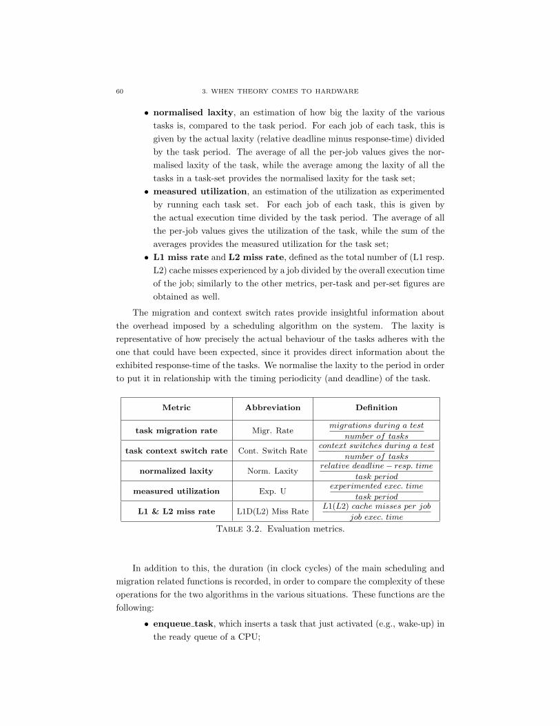
60 3. WHEN THEORY COMES TO HARDWARE
• normalised laxity, an estimation of how big the laxity of the various
tasks is, compared to the task period. For each job of each task, this is
given by the actual laxity (relative deadline minus response-time) divided
by the task period. The average of all the per-job values gives the nor-
malised laxity of the task, while the average among the laxity of all the
tasks in a task-set provides the normalised laxity for the task set;
• measured utilization, an estimation of the utilization as experimented
by running each task set. For each job of each task, this is given by
the actual execution time divided by the task period. The average of all
the per-job values gives the utilization of the task, while the sum of the
averages provides the measured utilization for the task set;
• L1 miss rate and L2 miss rate, defined as the total number of (L1 resp.
L2) cache misses experienced by a job divided by the overall execution time
of the job; similarly to the other metrics, per-task and per-set figures are
obtained as well.
The migration and context switch rates provide insightful information about
the overhead imposed by a scheduling algorithm on the system. The laxity is
representative of how precisely the actual behaviour of the tasks adheres with the
one that could have been expected, since it provides direct information about the
exhibited response-time of the tasks. We normalise the laxity to the period in order
to put it in relationship with the timing periodicity (and deadline) of the task.
Metric Abbreviation Definition
task migration rate Migr. Ratemigrations during a test
number of tasks
task context switch rate Cont. Switch Ratecontext switches during a test
number of tasks
normalized laxity Norm. Laxityrelative deadline− resp. time
task period
measured utilization Exp. Uexperimented exec. time
task period
L1 & L2 miss rate L1D(L2) Miss RateL1(L2) cache misses per job
job exec. time
Table 3.2. Evaluation metrics.
In addition to this, the duration (in clock cycles) of the main scheduling and
migration related functions is recorded, in order to compare the complexity of these
operations for the two algorithms in the various situations. These functions are the
following:
• enqueue task, which inserts a task that just activated (e.g., wake-up) in
the ready queue of a CPU;

3.5. EXPERIMENTAL RESULTS 61
• dequeue task, which removes a task that just deactivated (e.g. sleep)
from the ready queue of a CPU;
• pull tasks, which picks ready but not running tasks from remote run-
queues if they could run on the calling CPU;
• push tasks, which tries to send ready tasks that are not running on the
calling CPU to some other CPU where they would execute.
The performance metrics are gathered by using standard time and timer-related
of the GNU C Library6, by the Hardware Performance Counters and related tools
and libraries7 Functions durations in cycles are obtained by directly instrumenting
the functions inside the kernel.
3.5. Experimental Results
Running all the tests took several days, and yielded to an extensive set of
experimental data. In this section, an excerpt of such data is reported. The full
obtained data set (4.3GB in compressed form) is available for download from: http:
//retis.sssup.it/people/jlelli/papers/JSS2012. Statistics come from the
results of running 3 different randomly generated task sets for each configuration
in terms of scheduler, allocation policy, number of tasks and their WSS.
For example, one of the 3 task sets generated in the case of U=0.6 and 96
tasks is reported in Figure 3.4. Each point corresponds to a task with period and
utilisation as read from the X and Y coordinates of the point. The higher density of
points for lower periods is due to the logarithmic generation of the random periods.
0
0.2
0.4
0.6
0.8
1
10 20 30 40 50 60 70 80 90 100
Task u
tiliz
ation
Task period (ms)
Utilization limitTasks
Figure 3.4. One of the used task-sets with U=0.6 and 96 tasks.

62 3. WHEN THEORY COMES TO HARDWARE
U L1D L2 L1D L2
WSS 16KB WSS 256KB
0.6 0.086 0.138 4.238 0.145
0.7 0.082 0.126 4.244 0.131
0.8 0.081 0.120 4.233 0.124
Table 3.3. Cache behaviour with tasks from the task-sets exe-
cuted in isolation.
3.5.1. Running Each Task Alone
First, each task of each set has been executed in isolation at real-time priority
(the exact real-time scheduling policy has no impact) in order to get its “reference”
behaviour in terms of execution time and minimum cache misses. The obtained
cache miss figures, averaged for all of the task sets, are reported in Table 3.3. The
experimental variation of all the parameters is practically null due to the execution
in isolation of each individual task, thus it has not been shown. As it can be seen,
the cache-miss rates decrease when increasing the utilisation. In fact, longer jobs
exhibit a better chance to access hot-cache data in their activations. The trends
are similar for both cases of 16KB and 256KB WSS values.
3.5.2. Impact of Scheduling
Now for each configuration all the tasks in the task-set have been deployed
concurrently on the platform. In the following, the focus is on the configurations
with a WSS of 16KB. In all the shown results, the performance of EDF based and
RM based policies are numerically and visually compared.
Table 3.4 reports the obtained normalised laxity, measured U , context switch
rate, and migration rate for the various configurations: global (top table), clustered
(middle table) and partitioned (bottom table) scheduling, both with EDF and RM
policies. Each row corresponds to a different configuration with a total utilisation
and number of tasks as indicated in the first two columns. The reported numbers
constitute the average and standard deviation of the obtained metrics of interest
averaged across all the tasks and the 3 task sets corresponding to each configuration.
First, we focus on how the computation times changed in the various cases,
then the performance of the various scheduling algorithms from the application
viewpoint.
Comparing the same configurations under EDF and RM, the obtained context
switches under EDF are lower than under RM, with a tendency to have slightly
lower average context switches at high overall utilisation (0.8). On the other hand,
6More information is available at: http://www.gnu.org/software/libc.7More information at: http://en.wikipedia.org/wiki/Hardware_performance_
counter, http://icl.cs.utk.edu/papi/index.html and https://perf.wiki.kernel.
org.

3.5. EXPERIMENTAL RESULTS 63
U # Norm. Laxity Exp. U Cont. Switch Rate Migr. Rate
0.6
G-EDF G-RM G-EDF G-RM G-EDF G-RM G-EDF G-RM
96 0.637 ± 0.00 0.637 ± 0.00 0.714 ± 0.00 0.714 ± 0.00 7177.260 ± 204.66 7116.566 ± 320.55 1859.906 ± 43.87 1558.247 ± 62.43
144 0.742 ± 0.00 0.741 ± 0.01 0.755 ± 0.01 0.755 ± 0.01 6952.722 ± 351.99 6989.104 ± 205.90 2296.683 ± 182.73 1981.012 ± 225.60
192 0.790 ± 0.01 0.786 ± 0.01 0.806 ± 0.01 0.809 ± 0.01 7056.780 ± 297.99 7268.071 ± 297.61 3129.241 ± 132.60 2825.498 ± 289.64
0.7
G-EDF G-RM G-EDF G-RM G-EDF G-RM G-EDF G-RM
96 0.586 ± 0.01 0.585 ± 0.01 0.813 ± 0.00 0.814 ± 0.00 6942.156 ± 207.28 7099.365 ± 220.57 2062.438 ± 136.11 1988.503 ± 136.62
144 0.703 ± 0.01 0.700 ± 0.01 0.856 ± 0.00 0.859 ± 0.00 6956.086 ± 82.72 7159.338 ± 97.04 3158.907 ± 83.59 2865.542 ± 154.45
192 0.756 ± 0.01 0.560 ± 0.12 0.903 ± 0.01 0.909 ± 0.01 6689.106 ± 103.68 7112.031 ± 205.73 4365.604 ± 604.26 4201.139 ± 384.19
0.8
G-EDF G-RM G-EDF G-RM G-EDF G-RM G-EDF G-RM
96 0.408 ± 0.08 0.057 ± 0.27 0.919 ± 0.00 0.921 ± 0.00 7212.948 ± 78.86 7549.163 ± 79.46 3329.632 ± 37.64 3471.920 ± 42.39
144 0.246 ± 0.25 −1.277 ± 1.09 0.960 ± 0.01 0.964 ± 0.01 6447.051 ± 376.24 7209.424 ± 571.82 5261.287 ± 993.66 4944.606 ± 792.15
192 −17.268 ± 9.15 −10.330 ± 6.02 1.014 ± 0.01 1.016 ± 0.01 5879.139 ± 226.55 7146.064 ± 206.88 8088.148 ± 671.48 6886.774 ± 506.12
U # Norm. Laxity Exp. U Cont. Switch Rate Migr. Rate
0.6
C-EDF C-RM C-EDF C-RM C-EDF C-RM C-EDF C-RM
96 0.658 ± 0.01 0.659 ± 0.01 0.656 ± 0.00 0.656 ± 0.00 6772.528 ± 131.22 6838.740 ± 194.84 1612.500 ± 57.60 1499.889 ± 61.64
144 0.752 ± 0.02 0.749 ± 0.02 0.695 ± 0.01 0.695 ± 0.01 6500.192 ± 356.20 6698.641 ± 374.65 2038.775 ± 108.98 2029.683 ± 218.87
192 0.791 ± 0.02 0.787 ± 0.02 0.744 ± 0.01 0.746 ± 0.01 6550.771 ± 339.06 6979.425 ± 331.32 2600.418 ± 242.83 2571.901 ± 275.62
0.7
C-EDF C-RM C-EDF C-RM C-EDF C-RM C-EDF C-RM
96 0.604 ± 0.02 0.603 ± 0.02 0.750 ± 0.00 0.749 ± 0.00 6478.545 ± 254.34 6684.986 ± 213.21 1844.708 ± 129.20 1860.281 ± 116.97
144 0.706 ± 0.03 0.705 ± 0.02 0.792 ± 0.00 0.793 ± 0.00 6489.877 ± 302.18 6771.567 ± 248.40 2486.000 ± 98.06 2426.850 ± 86.98
192 0.750 ± 0.03 0.745 ± 0.03 0.838 ± 0.01 0.838 ± 0.01 6247.576 ± 86.31 6957.189 ± 127.15 2977.594 ± 160.47 3106.653 ± 148.02
0.8
C-EDF C-RM C-EDF C-RM C-EDF C-RM C-EDF C-RM
96 0.427 ± 0.09 0.367 ± 0.11 0.850 ± 0.00 0.849 ± 0.00 6472.833 ± 156.42 7016.882 ± 119.31 2259.243 ± 40.09 2475.653 ± 14.71
144 0.642 ± 0.05 0.220 ± 0.27 0.889 ± 0.01 0.890 ± 0.01 6045.720 ± 473.54 6751.257 ± 585.09 2995.255 ± 330.74 3135.801 ± 364.48
192 −0.017 ± 0.45 −0.470 ± 0.69 0.935 ± 0.01 0.935 ± 0.01 5834.167 ± 187.69 6868.012 ± 336.15 3766.528 ± 319.98 4011.521 ± 371.34
U # Norm. Laxity Exp. U Cont. Switch Rate Migr. Rate
0.6
P-EDF P-RM P-EDF P-RM P-EDF P-RM P-EDF P-RM
96 0.599 ± 0.04 0.598 ± 0.04 0.656 ± 0.00 0.656 ± 0.00 5895.493 ± 238.37 6246.983 ± 259.01 0.000 ± 0.00 0.000 ± 0.00
144 0.686 ± 0.05 0.684 ± 0.05 0.692 ± 0.01 0.693 ± 0.01 5575.343 ± 276.93 6006.002 ± 302.92 0.000 ± 0.00 0.000 ± 0.00
192 0.709 ± 0.06 0.707 ± 0.07 0.741 ± 0.01 0.741 ± 0.01 5560.694 ± 216.06 6132.670 ± 232.04 0.000 ± 0.00 0.000 ± 0.00
0.7
P-EDF P-RM P-EDF P-RM P-EDF P-RM P-EDF P-RM
96 0.526 ± 0.05 0.525 ± 0.04 0.748 ± 0.00 0.748 ± 0.00 5464.538 ± 254.98 5882.622 ± 226.24 0.000 ± 0.00 0.000 ± 0.00
144 0.617 ± 0.07 0.613 ± 0.06 0.789 ± 0.00 0.789 ± 0.00 5373.111 ± 154.76 5943.572 ± 42.84 0.000 ± 0.00 0.000 ± 0.00
192 0.633 ± 0.08 0.476 ± 0.21 0.834 ± 0.01 0.834 ± 0.00 5319.613 ± 122.86 6023.090 ± 219.59 0.000 ± 0.00 0.000 ± 0.00
0.8
P-EDF P-RM P-EDF P-RM P-EDF P-RM P-EDF P-RM
96 0.226 ± 0.19 −0.254 ± 0.42 0.847 ± 0.00 0.849 ± 0.00 5519.233 ± 167.03 6252.608 ± 67.19 0.000 ± 0.00 0.000 ± 0.00
144 0.537 ± 0.08 0.530 ± 0.07 0.885 ± 0.01 0.887 ± 0.01 5318.801 ± 417.72 5860.312 ± 431.40 0.000 ± 0.00 0.000 ± 0.00
192 −15.216 ± 8.93 −12.471 ± 6.76 0.929 ± 0.01 0.908 ± 0.03 4791.134 ± 184.04 5837.344 ± 170.43 0.000 ± 0.00 0.000 ± 0.00
Table 3.4. Statistics for the metrics of interest when
WSS=16KB, under various configurations: global (top table), clus-
tered (middle table) and partitioned (bottom table) scheduling,
both with EDF and RM policies.
the migration rates of EDF based policies are significantly higher than the ones of
RM based ones. However, the actual impact on the execution times of the tasks is
quite limited, as it can be observed by the experimental U measured (and averaged
over the 3 task sets available for each configuration) for EDF and RM based policies,
which are basically equivalent.
Comparing different configurations, the context switch rate decreases with the
load while, on the contrary, the migration rate increases (but decreases with the
WSS, not shown). Also, note that the average experimental utilisation increases

64 3. WHEN THEORY COMES TO HARDWARE
when switching from partitioned to clustered and then to global policies, as expected
due to the presence of migrations. This is also confirmed when looking at the
average execution times obtained for the individual tasks. For example, Figure 3.5
shows the ratio among the execution times obtained with global, clustered and
partitioned EDF scheduling, for the task set with U = 0.6 and 96 tasks shown also
in Figure 3.4, in the two cases of 16KB and 256KB WSS. As it can be seen, in the
cases of small WSS, clustered policies succeed in keeping the workload inflation at
contained and negligible amounts, as compared to global strategies. However, as the
WSS increases, the differences among the cache-related overheads of clustered and
global scheduling tend to vanish. Working very close to the L2 cache boundary, it
is very likely that each task has to reload a large part of its WSS when it is released,
independently from the processor it starts running on.
0.8
0.85
0.9
0.95
1
1.05
1.1
1.15
1.2
0 8 16 24 32 40 48 56 64 72 80 88 96
Execution tim
e r
atio
Task
C-EDF / P-EDF
G-EDF / P-EDF
0.8
0.85
0.9
0.95
1
1.05
1.1
1.15
1.2
0 8 16 24 32 40 48 56 64 72 80 88 96
Execution tim
e r
atio
Task
C-EDF / P-EDF
G-EDF / P-EDF
Figure 3.5. Execution times obtained for the various tasks (av-
eraged over the task activations) under C-EDF (plus signs) and
G-EDF (multiply signs) relative to the figures obtained under P-
EDF, in the cases of 16KB (top) and 256KB (bottom) WSS.
Now, let us observe how the various scheduler configurations impact the per-
formance as observable from within the applications themselves, i.e., let us focus
on the normalised laxity figures. The average figures obtained under EDF and RM
based policies are basically equivalent when the system load is low. This is due to
the fact that, when a task is favoured over another by the scheduler, then the former
will finish earlier and the latter will finish later, but when averaging figures this

3.5. EXPERIMENTAL RESULTS 65
difference is lost. The situation is different reaching the top edge with respect to
utilisation (i.e., U = 0.8) and number of tasks. Both EDF and RM policies exhibit
negative average laxity (tardiness) with 192 tasks, but only RM policies see this be-
haviour with also 92 and 144 tasks. It is furthermore evident that clustered policies
come out to be better from this viewpoint, as slight negative values appear with
192 tasks only; moreover, C-EDF outperforms C-RM with higher average laxity
figures.
In addition, let us look at the whole set of obtained laxity values, under various
scheduling policies, looking at their cumulative distribution functions (CDF), first
for the whole task set, then focusing on a few specific ones. Figure 3.6 shows the
obtained curves when the laxity of all the tasks is considered. It is evident that
(top sub-figure) global and clustered strategies (both for EDF and RM, first and
second curves) differ in a negligible way from each other, and that they tend to
lead to generally higher laxity values (better performance) than partitioned ones
(last two curves). Also, no difference can be appreciated between EDF and RM
from this viewpoint. However, zooming the figure in the critical area near a null
laxity (when the tasks are close to miss their deadlines), the differences between
the three policy types are more evident, with still global policies better than the
others. However, partitioned EDF from this viewpoint performs much better than
partitioned RM, and it achieves a similar performance to both clustered policies.
This difference is due to the particular task set and the way it has been partitioned
(nearly optimally – see Section 3.4.4) across CPUs. Also, it can be observed that
there is a certain amount of jobs missing their deadlines. However, these are below
1% of the total jobs that have been executed, with the exception of P-RM that
stands slightly above this value.
Now let us focus on the tasks with minimum period (there were 2 such tasks in
the experiment with a 10ms period), which have the most critical timing require-
ments, and the ones with maximum periods (there was 1 single task with a 98ms
period), which most often are preempted by lower period tasks. Figure 3.7 shows
the obtained CDF curves when only considering the normalised laxity of these two
subsets of tasks. It can be seen that global and clustered policies perform better
than the partitioned ones, with RM-based policies providing an exceptionally good
performance to the minimum-period tasks (Figure 3.7 top) at the expense of the
maximum-period ones (Figure 3.7 bottom). These are served very badly by G-
RM, while G-EDF achieves a borderline acceptable performance with nearly 18%
of deadline misses. However, the reduced overheads of clustered policies (see also
Section 4.4.3) show up clearly in this case, where both C-EDF and C-RM manage
to perform quite well.

66 3. WHEN THEORY COMES TO HARDWARE
0
0.2
0.4
0.6
0.8
1
0 0.1 0.2 0.3 0.4 0.5 0.6 0.7 0.8 0.9 1
Pr{
Laxity <
= x
}
x (ms)
16KB 0.8 96tsk G-EDF16KB 0.8 96tsk G-RM
16KB 0.8 96tsk C-EDF16KB 0.8 96tsk C-RM
16KB 0.8 96tsk P-EDF16KB 0.8 96tsk P-RM
0
0.05
0.1
0.15
0.2
0.25
0.3
0 0.1 0.2 0.3
Pr{
Laxity <
= x
}
x (ms)
16KB 0.8 96tsk G-EDF16KB 0.8 96tsk G-RM
16KB 0.8 96tsk C-EDF16KB 0.8 96tsk C-RM
16KB 0.8 96tsk P-EDF16KB 0.8 96tsk P-RM
Figure 3.6. CDF of the normalised laxity for all the tasks as ob-
tained under various scheduling policies, with U=0.8 and 96 tasks.
3.5.3. Working Set Size and Cache Behaviour
The impact of the WSS on the performance of the applications may be visually
compared by looking at Figure 3.8. It shows the laxity CDF curves achieved on
all the tasks for a WSS of 16KB (first two curves) and 256KB (last two curves),
zoomed in the critical area close to the deadline miss (null laxity), obtained in the
case of clustered EDF and RM scheduling, with U=0.8 and 96 tasks. Due to the
higher computation times experienced by tasks with a greater WSS, the achieved
laxity figures are correspondingly lower. In this plot, the difference between EDF
and RM policies cannot be appreciated (see comment on Figures 3.6 and 3.7 above).
In Table 3.5 (top), the number of cache misses for L1 and L2 caches are shown,
in the cases of global scheduling. They are higher than the case when tasks are run
in isolation (see Table 3.3), however still not so high. Also, the difference between
EDF and RM is negligible. In the middle sub-table, the figures for the cache misses
of the clustered policies are reported. The numbers are slightly greater than the case
of running the tasks in isolation, and very similar to the case of global scheduling
(top sub-table). In the bottom sub-table partitioned policies are shown. This time
the numbers are smaller than the global and clustered cases. This is due to the
absence of migrations.
As expected, the cache miss rate only marginally depends on the scheduling
algorithm. Rather, it has a strong dependency on the WSS, raising of one order of

3.5. EXPERIMENTAL RESULTS 67
0
0.2
0.4
0.6
0.8
1
0 0.1 0.2 0.3 0.4 0.5 0.6 0.7 0.8 0.9 1
Pr{
Laxity <
= x
}
x (ms)
16KB 0.8 96tsk G-EDF16KB 0.8 96tsk G-RM
16KB 0.8 96tsk C-EDF16KB 0.8 96tsk C-RM
16KB 0.8 96tsk P-EDF16KB 0.8 96tsk P-RM
0
0.2
0.4
0.6
0.8
1
0 0.1 0.2 0.3 0.4 0.5 0.6 0.7 0.8 0.9 1
Pr{
Laxity <
= x
}
x (ms)
16KB 0.8 96tsk G-EDF16KB 0.8 96tsk G-RM
16KB 0.8 96tsk C-EDF16KB 0.8 96tsk C-RM
16KB 0.8 96tsk P-EDF16KB 0.8 96tsk P-RM
Figure 3.7. CDF of the normalised laxity for the minimum-
period (top) and maximum-period (bottom) tasks, under various
scheduling policies, with U=0.8 and 96 tasks.
0
0.05
0.1
0.15
0.2
0.25
0 0.1 0.2 0.3
Pr{
Laxity <
= x
}
x (ms)
16KB 0.8 96tsk C-EDF16KB 0.8 96tsk C-RM
256KB 0.8 96tsk C-EDF256KB 0.8 96tsk C-RM
Figure 3.8. CDF of the obtained normalised laxity for clustered
EDF and RM policies with WSS of 16KB and 256KB, with U=0.8
and 96 tasks.
magnitude when switching from a WSS of 16KB to one of 256KB. From the 16KB
WSS tables, it might seem that clustering policies lead to higher cache miss rates
than global scheduling, which is counter-intuitive. However, the differences are
really small and sometimes within the variability range attested by the measured
standard deviation. Also, for the 256KB WSS cases, partitioned policies seem to
experience fewer cache misses than the others, but this is true for L1D cache miss

68 3. WHEN THEORY COMES TO HARDWARE
U Algo. L1D Miss Rate L2 Miss Rate L1D Miss Rate L2 Miss Rate
WSS 16KB WSS 256KB
0.6G-EDF 0.100 ± 0.02 0.085 ± 0.05 4.405 ± 0.04 0.163 ± 0.07
G-RM 0.099 ± 0.03 0.091 ± 0.05 4.392 ± 0.04 0.171 ± 0.07
0.7G-EDF 0.101 ± 0.03 0.069 ± 0.04 4.421 ± 0.05 0.154 ± 0.06
G-RM 0.098 ± 0.03 0.072 ± 0.04 4.352 ± 0.04 0.157 ± 0.06
0.8G-EDF 0.119 ± 0.05 0.056 ± 0.03 4.808 ± 0.07 0.169 ± 0.07
G-RM 0.103 ± 0.03 0.050 ± 0.02 4.344 ± 0.05 0.156 ± 0.05
U Algo. L1D Miss Rate L2 Miss Rate L1D Miss Rate L2 Miss Rate
WSS 16KB WSS 256KB
0.6C-EDF 0.107 ± 0.03 0.101 ± 0.06 4.475 ± 0.04 0.173 ± 0.07
C-RM 0.107 ± 0.03 0.096 ± 0.05 4.467 ± 0.04 0.178 ± 0.07
0.7C-EDF 0.104 ± 0.02 0.083 ± 0.05 4.479 ± 0.04 0.159 ± 0.06
C-RM 0.102 ± 0.02 0.079 ± 0.05 4.472 ± 0.04 0.165 ± 0.06
0.8C-EDF 0.108 ± 0.03 0.064 ± 0.04 4.493 ± 0.05 0.153 ± 0.06
C-RM 0.105 ± 0.02 0.061 ± 0.03 4.464 ± 0.04 0.163 ± 0.05
U Algo. L1D Miss Rate L2 Miss Rate L1D Miss Rate L2 Miss Rate
WSS 16KB WSS 256KB
0.6P-EDF 0.095 ± 0.02 0.060 ± 0.03 4.504 ± 0.03 0.125 ± 0.03
P-RM 0.093 ± 0.02 0.059 ± 0.03 4.505 ± 0.03 0.127 ± 0.03
0.7P-EDF 0.090 ± 0.01 0.048 ± 0.02 4.529 ± 0.03 0.109 ± 0.02
P-RM 0.088 ± 0.01 0.048 ± 0.02 4.506 ± 0.03 0.116 ± 0.03
0.8P-EDF 0.087 ± 0.01 0.038 ± 0.02 4.787 ± 0.03 0.104 ± 0.02
P-RM 0.088 ± 0.01 0.040 ± 0.02 4.502 ± 0.03 0.119 ± 0.03
Table 3.5. Cache related behaviour of global (top sub-table),
clustered (middle sub-table) and partitioned (bottom sub-table)
EDF and RM policies for various configurations (values are averages
of all the runs for each configuration) and WSS.
rates only. Since the WSS exceeds the L1D border, little can be said about the L1D
behaviour. Instead, partitioning policies lead to the lowest L2 cache miss rates as
expected.
3.5.4. Scheduling Overheads Comparison
In this paragraph, the scheduling overheads obtained under various policies are
compared, using the metrics described in Section 3.4.5
In Table 3.6, the overheads obtained in various configurations with a WSS of
16KB are reported. All numbers are expressed in clock cycles.
EDF based policies consistently present lower number of cycles than RM ones
for enqueue operations, while, on the contrary, this is true for the partitioned case
only for dequeue operations. The difference in performance is due to the completely
different data structures used in the two cases. Concerning the pull operations, in
the global and clustered scheduling cases the overheads of EDF are about twice or
three times the ones of RM, whilst in the partitioned cases they are both null. Note
that the small numbers shown as overheads of pull operations in the partitioned case
are due to the few migrations at the beginning of the experiment needed to deploy
the tasks over the assigned cores. Looking at the push operations, the overheads of

3.6. CONCLUSIONS 69
U # Enqueue mean time Dequeue mean time Push mean time Pull mean time
0.6
G-EDF G-RM G-EDF G-RM G-EDF G-RM G-EDF G-RM
96 4099 ± 104.1 4867 ± 72.3 4672 ± 370.0 4518 ± 32.6 13444 ± 952.6 13895 ± 192.8 13689 ± 3772 4905 ± 124.6
144 4147 ± 148.4 5298 ± 377.4 5158 ± 266.6 4719 ± 114.0 12637 ± 603.0 12310 ± 1018 30775 ± 4081 9143 ± 954.0
192 4078 ± 185.1 5304 ± 248.7 5803 ± 57.2 4740 ± 135.8 11938 ± 320.9 10705 ± 913.9 54308 ± 1236 15379 ± 1063
0.7
G-EDF G-RM G-EDF G-RM G-EDF G-RM G-EDF G-RM
96 3977 ± 297.0 4810 ± 146.2 4304 ± 22.2 4183 ± 68.3 11836 ± 832.9 11743 ± 425.0 11299 ± 1398 6635 ± 859.9
144 3840 ± 56.2 5006 ± 356.1 5288 ± 39.3 4309 ± 56.1 9674 ± 495.2 9144 ± 460.1 35216 ± 3847 13480 ± 534.9
192 3740 ± 132.8 4985 ± 220.0 5833 ± 333.4 4239 ± 83.0 8469 ± 497.5 7610 ± 478.0 64636 ± 13444 23708 ± 2175
0.8
G-EDF G-RM G-EDF G-RM G-EDF G-RM G-EDF G-RM
96 3516 ± 108.6 4295 ± 174.1 4338 ± 221.8 3796 ± 16.8 7056 ± 299.3 7250 ± 175.5 15072 ± 2540 13278 ± 131.7
144 3367 ± 23.0 4391 ± 49.1 5317 ± 66.9 3896 ± 75.9 5428 ± 390.6 5917 ± 362.3 42396 ± 5308 24977 ± 2114
192 3420 ± 136.3 4531 ± 80.2 6172 ± 266.2 3965 ± 34.8 5830 ± 514.9 5872 ± 131.8 102436 ± 14741 40633 ± 2124
U # Enqueue mean time Dequeue mean time Push mean time Pull mean time
0.6
C-EDF C-RM C-EDF C-RM C-EDF C-RM C-EDF C-RM
96 3857 ± 207.8 4961 ± 86.2 4531 ± 34.4 4552 ± 59.7 7388 ± 295.0 8840 ± 593.0 15726 ± 1143 11367 ± 1316
144 3742 ± 98.7 5006 ± 268.1 4920 ± 75.0 4523 ± 53.6 6154 ± 195.5 7442 ± 88.4 33045 ± 2679 19974 ± 2637
192 3864 ± 164.6 5056 ± 178.3 5465 ± 147.2 4533 ± 97.6 5271 ± 408.8 6631 ± 160.8 71980 ± 12418 31313 ± 6240
0.7
C-EDF C-RM C-EDF C-RM C-EDF C-RM C-EDF C-RM
96 3519 ± 125.7 4568 ± 192.2 4388 ± 108.2 4292 ± 23.1 6074 ± 683.1 7356 ± 152.9 17161 ± 2258 15319 ± 1646
144 3592 ± 164.7 4487 ± 246.4 5102 ± 219.6 4185 ± 62.4 4837 ± 278.9 6712 ± 357.4 44885 ± 2780 24738 ± 1861
192 3658 ± 97.2 4925 ± 210.3 5576 ± 172.9 4377 ± 48.7 4022 ± 345.6 6144 ± 657.8 81507 ± 14115 40518 ± 2069
0.8
C-EDF C-RM C-EDF C-RM C-EDF C-RM C-EDF C-RM
96 3295 ± 34.1 4326 ± 99.5 4348 ± 127.6 3874 ± 70.8 4139 ± 217.4 6108 ± 149.2 20888 ± 1987 18963 ± 105.9
144 3310 ± 155.6 4375 ± 309.3 5001 ± 171.6 3981 ± 121.8 3066 ± 319.7 5667 ± 236.2 50546 ± 5266 33437 ± 2427
192 3384 ± 30.2 4616 ± 105.0 5563 ± 108.3 4095 ± 81.2 2382 ± 152.2 4821 ± 138.2 90440 ± 7631 52870 ± 3211
U # Enqueue mean time Dequeue mean time Push mean time Pull mean time
0.6
P-EDF P-RM P-EDF P-RM P-EDF P-RM P-EDF P-RM
96 3159 ± 225.0 4347 ± 213.3 4089 ± 57.9 5309 ± 85.7 0.0 ± 0.0 0.0 ± 0.0 131.0 ± 2.5 168.6 ± 6.2
144 2956 ± 172.8 4106 ± 174.2 4094 ± 42.9 5397 ± 142.5 0.0 ± 0.0 0.0 ± 0.0 132.1 ± 3.2 124.2 ± 34.6
192 2751 ± 145.6 3997 ± 259.5 4014 ± 82.1 5375 ± 81.9 0.0 ± 0.0 0.0 ± 0.0 130.2 ± 7.9 121.1 ± 14.4
0.7
P-EDF P-RM P-EDF P-RM P-EDF P-RM P-EDF P-RM
96 3471 ± 530.6 4025 ± 375.5 3990 ± 25.8 5251 ± 159.3 0.0 ± 0.0 0.0 ± 0.0 127.5 ± 4.5 151.1 ± 12.0
144 2541 ± 171.3 3898 ± 516.0 3962 ± 157.9 5372 ± 128.4 0.0 ± 0.0 0.0 ± 0.0 126.2 ± 9.6 124.8 ± 1.2
192 2363 ± 121.5 3375 ± 152.5 3879 ± 37.9 5352 ± 106.1 0.0 ± 0.0 0.0 ± 0.0 119.0 ± 3.7 103.6 ± 10.2
0.8
P-EDF P-RM P-EDF P-RM P-EDF P-RM P-EDF P-RM
96 2754 ± 143.4 3884 ± 140.8 3847 ± 84.3 5087 ± 63.3 0.0 ± 0.0 0.0 ± 0.0 126.9 ± 5.2 96.8 ± 8.4
144 2530 ± 29.6 3471 ± 143.4 3886 ± 44.9 5231 ± 115.4 0.0 ± 0.0 0.0 ± 0.0 115.9 ± 2.0 91.4 ± 11.1
192 2156 ± 112.6 3796 ± 536.2 3598 ± 43.5 4995 ± 88.0 0.0 ± 0.0 0.0 ± 0.0 109.1 ± 0.9 82.5 ± 2.7
Table 3.6. Scheduling and migration related function durations
(on average, in clock cycles) for global (top sub-table), clustered
(middle sub-table) and partitioned (bottom sub-table) EDF and RM
policies, in the case of WSS=16KB.
G-EDF and G-RM are comparable, while C-EDF exhibits less overhead numbers
than C-RM. These kind of results were expected, since in [?] only push operations
were addressed, making them efficient.
3.6. Conclusions
In this chapter, an experimental comparison of various multi-processor schedul-
ing algorithms has been performed by running synthetic workloads of real tasks on

70 3. WHEN THEORY COMES TO HARDWARE
a Linux system. The performance of the various solutions has been evaluated under
diverse metrics and under multiple combinations of CPU utilisation and number of
tasks.
The experimental results lead to some interesting considerations. It appears
clear that global and clustered algorithms are a viable solution for multi-core plat-
forms with a high degree of cache sharing, mainly because the overhead caused
by migrations is not more costly than a “traditional” context switch. Partitioned
scheduling requires a potentially costly operation of allocation of tasks to cores,
and it may not manage to make use of the whole computing power available on a
system. On the other hand, global scheduling has the ability to perform automatic
load balancing dynamically at run-time, achieving better normalised laxity figures.
However, with a large number of cores, true global scheduling may lead to a growth
in overheads that needs to be kept under control, whilst clustered scheduling ap-
proaches may perform better thanks to their reduced overheads, especially when
the tasks have been properly/optimally partitioned across the clusters. Indeed, at
reduced sizes of the tasks WSS, clustered algorithms manage to keep applications
data in the cache shared among the cores in a cluster (if present), thus achieving
very little migration costs, as compared to what happens with global strategies.
However, the difference tends to vanish when the WSS grows.
It is important to compare our results with the ones in [BBA10a], where the
authors concluded that “G-EDF is never a suitable policy for hard RT systems”.
This may seem in conflict with our conclusions about the viability of global schedul-
ing for RT systems. First, the reader will notice that the former conclusions concern
hard real-time systems, where a formal assessment on the obtainable performance
(and existence of deadline misses) can only be obtained via proper schedulability
analysis techniques. On the other hand, our conclusions derive from observations
of the actual behaviour of the tasks as scheduled on a real OS over a certain time
horizon. In this regard, it is useful to observe that all of the task sets used in the
experiments shown in our comparison have been found as non-schedulable accord-
ing to one [BC07] of the tests for G-EDF which is known to be among the best
known [BB10]. Second, it was not possible to set-up an experiment exactly identi-
cal to the one(s) in [BBA10a], due to the unavailability of the whole used data set
(task WCETs, periods and clusters/partitions). Third, the analysis in [BBA10a]
relies on the weighted schedulability, computed over task-sets with heterogeneous
overall utilisation, obtained as a weighted average of the percentages of schedulable
task-sets, obtained using the utilisation itself as weight. This metric was not mean-
ingful in our context, because we were not interested in schedulability as assessed
by a conservative analysis technique, but rather in the soft real-time performance as
observed from the running system. On a related note, all of the task sets we consid-
ered were not schedulable by G-EDF, as stated above. Finally, another difficulty in

3.6. CONCLUSIONS 71
comparing the two approaches is due to the differences in the actual task body and
in the underlying physical platform, which cause differences in the cache behaviour
of the tasks when deployed on the various cores under the various configurations.
As a further remark, in both cases the conclusions cannot be considered abso-
lutely generic, because they derive from the use of a limited number of randomly
generated task sets.
In view of complete transparency, we have to state it clear that it was not pos-
sible (for practical reasons) to run the task sets till the hyper-period (even though
the experiments duration was tuned so as to allow for a number of activations of
each task between 600 and 6000, depending on their periods). Therefore, the re-
ported measurements are referred to a limited observation horizon over each task-set
schedule, and cannot be considered to be completely exhaustive of each and every
possible foreseeable behaviour under the considered scheduling algorithms. Still,
we believe the results reported in this chapter are very useful for soft real-time sys-
tems, where the main focus in on how applications may behave most of the times,
and the actual worst-case that may show up once in a while may merely lead to
temporary degradations of the provided service that can be easily tolerated by the
system (and final users).
The implementation of G-EDF used to perform the evaluation presents accept-
able overhead figures in terms of durations of the scheduling functions, being com-
parable with the corresponding ones present in the standard fixed priority scheduler
of the Linux kernel. The performed evaluation highlights that such overheads grow
anyway with the number of cores over which one is globally scheduling. Clustered
policies lead to most of the benefits of global ones, and they can actually perform
better thanks to the reduced overhead figures, posing the foundations for scalability
of the technique to a high number of cores. The cost to pay is again the need for
allocating tasks to clusters. However, such problem comes in a much more reduced
form than the one of allocating to cores.


CHAPTER 4
Resource Reservation & Shared Resources on
SMP
4.1. Introduction
In the previous chapters we detailed about our implementation of a resource
reservation mechamism that can be used to provide timeliness guarantees to non-
interacting real-time activities. In this chapter we start deadling with problems
that arise when concurrent real-time task interacts using shared data. In this case,
priority inheritance mechanims permit the donation of priorities between inter-
acting tasks, thus allowing runtime guarantees to be provided to groups of tasks
sharing data in mutual exclusion. Unfortunately, resource reservation mechanisms
are incompatible with classical resource access protocols like priority inheritance.
This has been shown in [LLA04]: if the budget is exhausted while the thread is
executing inside a critical section, the priority inversion of blocked tasks can grow
arbitrarily large. The authors proposed an extension of the priority inheritance
protocol, called Bandwidth Inheritance BWI [LLA04], in which the thread that
holds the lock inherits not only the priority but also the budget of the blocked tasks.
The protocol has recently been extended to multi-processor systems, thus becoming
the Multi-processor Bandwidth Inheritance (M-BWI) protocol [FLC12], and it has
been implemented in LITMUS-RT [LIT], a research-oriented OS designed to make
it easy to implement and evaluate new scheduling policies. However, LITMUS-RT
is not particularly optimized for use in production systems, and it is not up-to-date
with respect to current Linux OS releases.
In this Chapter we detail about an implementation of the M-BWI protocol
in Linux patched with SCHED DEADLINE. We explain the architecture and the
practical aspects of our implementation. Also, we present the problems that we
encountered, and a few solutions to them. Finally, we present the evaluation of the
overhead introduced by the protocol.
4.2. State of the art
4.2.1. Model of a critical section
Tasks can access shared memory using mutually exclusive semaphores, often
referred to as mutexes. The portion of code in a task between a lock and an unlock
73
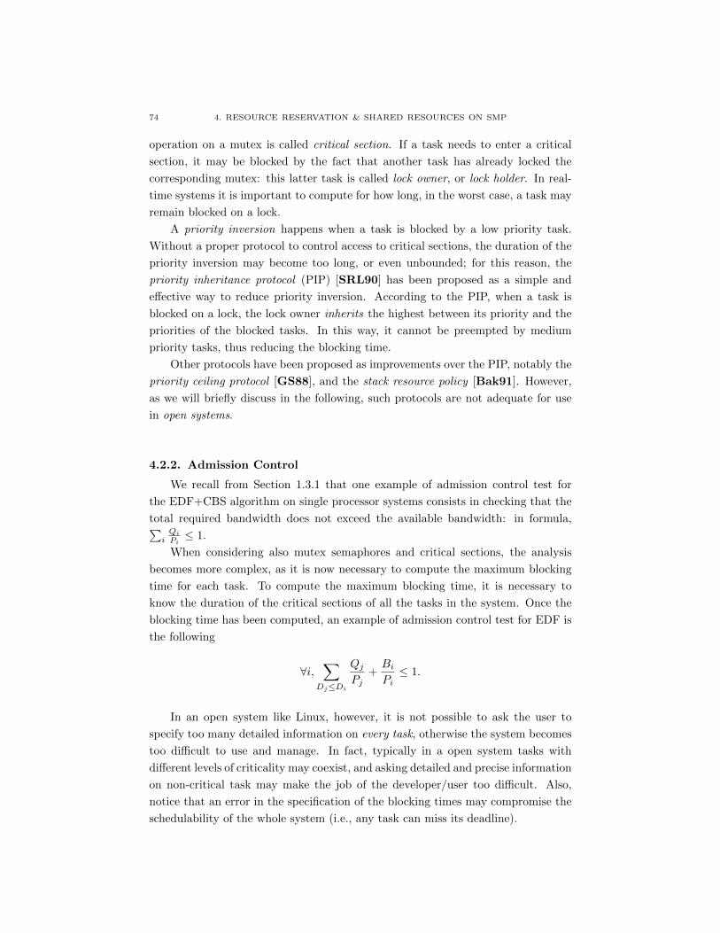
74 4. RESOURCE RESERVATION & SHARED RESOURCES ON SMP
operation on a mutex is called critical section. If a task needs to enter a critical
section, it may be blocked by the fact that another task has already locked the
corresponding mutex: this latter task is called lock owner, or lock holder. In real-
time systems it is important to compute for how long, in the worst case, a task may
remain blocked on a lock.
A priority inversion happens when a task is blocked by a low priority task.
Without a proper protocol to control access to critical sections, the duration of the
priority inversion may become too long, or even unbounded; for this reason, the
priority inheritance protocol (PIP) [SRL90] has been proposed as a simple and
effective way to reduce priority inversion. According to the PIP, when a task is
blocked on a lock, the lock owner inherits the highest between its priority and the
priorities of the blocked tasks. In this way, it cannot be preempted by medium
priority tasks, thus reducing the blocking time.
Other protocols have been proposed as improvements over the PIP, notably the
priority ceiling protocol [GS88], and the stack resource policy [Bak91]. However,
as we will briefly discuss in the following, such protocols are not adequate for use
in open systems.
4.2.2. Admission Control
We recall from Section 1.3.1 that one example of admission control test for
the EDF+CBS algorithm on single processor systems consists in checking that the
total required bandwidth does not exceed the available bandwidth: in formula,∑iQi
Pi≤ 1.
When considering also mutex semaphores and critical sections, the analysis
becomes more complex, as it is now necessary to compute the maximum blocking
time for each task. To compute the maximum blocking time, it is necessary to
know the duration of the critical sections of all the tasks in the system. Once the
blocking time has been computed, an example of admission control test for EDF is
the following
∀i,∑
Dj≤Di
QjPj
+BiPi≤ 1.
In an open system like Linux, however, it is not possible to ask the user to
specify too many detailed information on every task, otherwise the system becomes
too difficult to use and manage. In fact, typically in a open system tasks with
different levels of criticality may coexist, and asking detailed and precise information
on non-critical task may make the job of the developer/user too difficult. Also,
notice that an error in the specification of the blocking times may compromise the
schedulability of the whole system (i.e., any task can miss its deadline).

4.2. STATE OF THE ART 75
Figure 4.1. A task exhaust its budget while in a critical section,
thus increasing the blocking time of another task.
4.2.3. Combining resource reservations and critical sections
When trying to combine resource reservations with a resource access protocol,
we need to solve two problems. The first problem is concerned with how to take
into account blocking time in the admission control formula, as described in the
previous section.
The second problem is concerned with handling the situation that occurs when a
task is in a critical section and its budget is exhausted. In that case, the scheduler
algorithm throttles the task (i.e., suspends it) until the next period, when the
budget is recharged to its maximum value. However, another task blocked on the
semaphore must also wait for the budget to recharge. Therefore, the worst case
blocking time may become very large.
An example of such situation is depicted in Figure 4.1, where task τ1 suffers
a long blocking time from τ3 whose budget is exhausted at time t = 4 while in a
critical section on mutex M.
We want to avoid this problem. At the same time, we would like to avoid
the necessity to compute the blocking time of non critical tasks, and maintain the
useful property of temporal isolation. So, the goals for our resource access protocol
are the following
(1) We shall not require the user to specify any parameter to run the task,
other that the desired budget and period (Q,P );
(2) Temporal protection: the performance of a task (i.e., its ability to meet
its deadline) shall depend only on its parameters (Q,P ), on its worst-case
execution time and period, and on the duration of the critical sections of
the tasks with which it interacts;
(3) If we do know the worst-case execution times (and duration of critical
sections) of the task and of all interacting tasks, it must be possible to
compute (Q,P ) such that the task will meet its deadline;

76 4. RESOURCE RESERVATION & SHARED RESOURCES ON SMP
(4) We want to do this on multi-core systems as well.
4.2.4. Interacting tasks
What do we mean with interacting tasks? In the simplest case, we say that two
tasks interact when they access a critical section with the same mutex. However,
since critical sections can be nested within each other, the general case is a little
more complex.
A blocking chain from a task τi to a task τj is a sequence of alternating tasks
and semaphores:
Hi,j = {τi → Ri,1 → τi,1 → Ri,2 → . . .→ Ri,ν → τj}
such that τj is the lock owner on semaphore Ri,ν and τi is blocked on Ri,1. As an
example, consider the blocking chain H1,3 = {τ1 → R1 → τ2 → R2 → τ3}, in which
τ3 accesses R2, τ2 accesses R2 with a cs nested inside cs on R1, τ1 accesses R1.
We say that a task τj interferes with task τi only if a blocking chain from τi
to τj exists. We say that task τi is independent of, or temporally isolated from τj
when there exist no blocking chain from τi to τj . We would like to maintain the
temporal isolation property:
The ability of a task to meet its deadlines depends only on its
worst-case computation time and arrival pattern, its assigned
budget and period, and the duration of the critical sections in
the blocking chains starting from τi.
4.2.5. The M-BWI protocol
We informally describe here the rules of the algorithm. A more complete and
detailed description can be found in [FLC12].
• When a task is blocked on a mutex we have several cases:
– if the lock-owner is itself blocked, the blocking chain is followed until
a non-blocked lock-owner is found;
– if the lock-owner is executing on another processor, the blocking task
actively waits for the lock owner to release the mutex;
– if the lock-owner is not executing, then it inherits the budget and
scheduling deadline of the blocked task.
• Therefore, when holding the lock on a mutex, a task can have a list of
pairs (budget,deadline) that it can use; it will always execute consuming
the budget of the earliest deadline pair.
• When a task releases the mutex, it will discard the pairs of (budget,deadline)
of the blocked tasks from its list.
Rather than going through a formal analysis of the protocol, we will present
here one example that demonstrate how the protocol works. In Figure 4.2 we show
the schedule produced by three tasks scheduled on 2 processors with migration. All
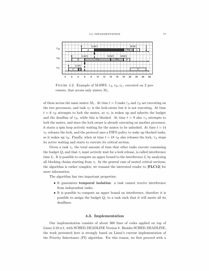
4.3. IMPLEMENTATION 77
Figure 4.2. Example of M-BWI: τA, τB , τC , executed on 2 pro-
cessors, that access only mutex M1.
of them access the same mutex M1. At time t = 5 tasks τA and τB are executing on
the two processors, and task τC is the lock-owner but it is not executing. At time
t = 6 τB attempts to lock the mutex, so τC is woken up and inherits the budget
and the deadline of τB , while this is blocked. At time t = 9 also τA attempts to
lock the mutex, and since the lock owner is already executing on another processor,
it starts a spin loop actively waiting for the mutex to be unlocked. At time t = 14
τC releases the lock, and the protocol uses a FIFO policy to wake up blocked tasks,
so it wakes up τB . Finally, when at time t = 18 τB also releases the lock, τA stops
its active waiting and starts to execute its critical section.
Given a task τi, the total amount of time that other tasks execute consuming
the budget Qi and that τi must actively wait for a lock release, is called interference
time Ii. It is possible to compute an upper bound to the interference Ii by analyzing
all blocking chains starting from τi. In the general case of nested critical sections,
the algorithm is rather complex; we remand the interested reader to [FLC12] for
more information.
The algorithm has two important properties:
• It guarantees temporal isolation: a task cannot receive interference
from independent tasks;
• It is possible to compute an upper bound on interference, therefore it is
possible to assign the budget Qi to a task such that it will meets all its
deadlines.
4.3. Implementation
Our implementation consists of about 300 lines of codes applied on top of
Linux 3.10-rc1, with SCHED DEADLINE Version 8. Besides SCHED DEADLINE,
the work presented here is strongly based on Linux’s current implementation of
the Priority Inheritance (PI) algorithm. For this reason, we first proceed with a

78 4. RESOURCE RESERVATION & SHARED RESOURCES ON SMP
(incomplete) review of Linux’s PI design and implementation 1, and then with the
detailed description of our contribution. The reader which already knows about
Linux’s PI infrastructure may want to skip the next subsection.
The terms task and process are used interchangeably in the rest of the docu-
ment.
4.3.1. Priority Inheritance in Linux
Basic structures
In the following discussion, we will be adopting the following terminology:
Mutex.: A mutex semaphore which is shared by the processes and by which
processes may interact and synchronize. The mutex structure contains a
pointer to the owner of the mutex. If the mutex is not owned, this pointer
is set to NULL.2
PI chain.: It is the same as the blocking chain defined in Section 4.2.4, i.e.
an alternating series of mutexes and processes such that each process in
the chain is blocked on the next mutex in the chain (if any), and it is
the owner the previous one in the chain (if any). The PI chain causes
processes to inherit priorities from a previous process that is blocked on
some of its mutexes.
Lock.: A spin-lock that is used to protect parts of the PI algorithm. These
locks disable preemption on uni-processors and prevent multiple CPUs
from entering critical sections simultaneously on SMPs.
Waiter.: A structure, stored on the stack of a blocked task, that holds a
pointer to the process, as well as the mutex that the task is blocked on.
It also contains the node structures to place the task in the right place
within the PI chains. More on this below.
Top waiter: The highest priority process waiting on a mutex.
Top PI waiter: The highest priority process waiting on one of the mutexes
that a specific process owns.
Since a process may own more than one mutex, but can never be blocked on more
than one, PI chains can merge at processes. Also, since a mutex may have more
than one process blocked on it, but never be owned by more than one, we can have
multiple chains merge on mutexes.3
In order to store the PI chains, Linux adopts two priority-sorted linked lists:
1Documentation/rt-mutex-design.txt2Linux actually implements a more involved mechanism that considers “Pending Own-
ership” and “Lock Stealing”.3The maximum depth of the PI chain is not dynamic and can actually be defined by
an static analysis of the code.
4.3. IMPLEMENTATION 79
Waiter list.: Every mutex keeps track of all the waiters that are blocked on
it by storing them in its waiter list. This list is protected by a lock called
wait lock. Since no modification of the waiter list is done in an interrupt
context, the wait lock can be taken without disabling interrupts.
PI list: Each process stores the top waiters of the mutexes that are owned
by the process in its PI list. Note that, in general, this list does not hold
all the waiters that are blocked on these mutexes. The list is protected by
a lock called PI lock. This lock may also be taken in interrupt context, so
when locking the PI lock, interrupts must be disabled.
The top of the task’s PI list is always the highest priority task that is waiting on
a mutex that is owned by the task. So if the task has inherited a priority, it will
always be the priority of the task that is at the top of this list.
Priority adjustments
In the implementation of the priority inheritance protocol, there are several
different locations in the code where a process must adjust its priority. With the
help of the PI list it is rather easy to know what need to be adjusted; we now
describe in more detail the main functions involved in this process.
The function that is responsible for adjusting the priority of a given task is
__rt_mutex_ adjust_prio. The function first obtains the priority that the task
should have, that is either the task’s own normal priority, or the priority of a
higher priority process that is waiting on a mutex owned by the task. By the above
discussion, this is simply a matter of comparing the priority of the top PI waiter’s
with the task’s normal priority. The function then examines the result, and if this
does not match the task’s current priority, the task’s scheduling class methods are
called to implement the actual change in priority.
Note that __rt_mutex_adjust_prio can either increase or decrease the priority
of the task. In the case that a higher priority process has just blocked on a mutex
owned by the task, the function would increase (or boost) the task’s priority. But
if a higher priority task were for some reason to leave the mutex (e.g., timeout or
signal), this same function would decrease (or unboost) the priority of the task.
This is because the PI list always contains the highest priority task that is waiting
on a mutex owned by the task.
When the function __rt_mutex_adjust_prio is performed on a task, the nodes
of the task’s waiter are not updated with the new priority, therefore this task may
not be in the proper locations in the waiter list of the mutex the task is blocked on
and in the PI list of the corresponding owner. The function rt mutex adjust prio
chain solves all this: it walks along the PI chain originating from the task, and
updates nodes and priorities of each process it finds.
The PI chain walk can be a time-consuming operation; for this reason, rt mutex
adjust prio chain not only defines a maximum lock depth, but it also only holds

80 4. RESOURCE RESERVATION & SHARED RESOURCES ON SMP
at most two different locks at a time, as it walks the PI chain (this means that the
state of the PI chain can change while in rt_mutex_adjust_prio_chain). When
the function is called no locks is held. Then, roughly, a loop is entered where:
(1) the PI lock of the task is taken to prevent more changes to its PI list;
(2) if the task is not blocked on a mutex, the loop is exited (we are at the top
of the PI chain); otherwise the wait lock of the mutex is taken to update
the task’s node location in the wait list;
(3) the PI lock of the task is released, and the PI lock of the mutex’s owner is
taken to update the task’s node location in the PI list of the new process;
(4) the PI lock of the previous owner and the wait lock of the mutex are
released; a new iteration of the loop is started where the previous owner
will be the next task to be processed.
4.3.2. The implementation of M-BWI
The majority of our modifications (and of the difficulties we found, see be-
low) consists in the integration of the SCHED DEADLINE patch described in Sec-
tion 2.2, with Linux’s PI infrastructure described in Section 4.3.1. Indeed, at this
time SCHED DEADLINE only implements an approximated version of deadline-
inheritance, in which the relative deadlines of the tasks are inherited but without
control on the corresponding bandwidths; on the other hand, the implementation
of PI was designed and optimized for fixed-priority tasks, hypothesis which can not
be assumed for tasks scheduled with SCHED DEADLINE policy.
In the course of our work, we have tried to keep at the minimum the modi-
fications to original data structures in Linux and in SCHED DEADLINE, and to
maintain the original functions’ semantics. For these reasons, our implementation
deviates from the original M-BWI protocol as described in section 4.2.5, in that it
does not consider tasks busy-waiting: like for PI, a lock-holding task inherits the
scheduling parameters of a blocked task, either if the lock-holding task is executing
or not.
Structures
As mentioned in section 4.3.1, Linux implements the waiter and the PI lists
using priority-sorted linked lists. These are linked lists suitable to sort processes
with fixed priorities; unlike ordinary lists, the head of this list is a different element
than the nodes of the list. On the other hand, the version of deadline-inheritance
which comes with SCHED DEADLINE replaces these priority-sorted linked lists
with red-black trees ordered by (absolute) deadline.
Our implementation adopts these structures to store chains of tasks and mu-
texes (that we will continue to call PI chains) so that it can keep the list of servers
that a task can inherit sorted accordingly. By caching the left-most node of the

4.3. IMPLEMENTATION 81
tree, it takes O(1) to retrieve the highest priority (earliest deadline) task in the list,
as for Linux’s priority-sorted linked-lists.
A pointer of type sched_dl_entity (the scheduling entity for SCHED DEAD-
LINE task) has been added to each sched_dl_entity structure. This pointer,
named bwi, is required to store the effective scheduling parameters (deadline and
capacity) of a SCHED DEADLINE task, and it will point either to the task’s de-
fault scheduling entity or, if a waiter with earlier deadline exists in the task’s PI
list, to the scheduling entity of the task’s top PI waiter. In either cases, we will
called the scheduling entity pointed by bwi the inherited scheduling entity or the
inherited server.
We note that this terminology is not completely consistent with the one in
[LLA01], even if the net result is the same. In the original presentation, each
process “inherits” all the servers in its PI list, and it can execute in any of them;
the CBS algorithm will then select the server (and the only runnable task within
the server) with the earliest deadline. For the scope of this document, the inherited
server, or the inherited scheduling parameters, will be this last. The difference in the
terminology is mainly due to the fact that nor Linux neither SCHED DEADLINE
provide us with a server structure, and to the fact that SCHED DEADLINE stores
the server parameters in the scheduling entity of the task.
Functions
Linux resorts to the PI’s logic (priority adjustments and chain walks) each
time an event occurs that can possibly result in a PI chain modification. Common
examples are the blocking of a task on a mutex, the release of a mutex, or the
explicit call to a system call that can modify the priority and the scheduling class
of a task (sched_setscheduler, sched_setparam). This remains true in the case
of M-BWI for SCHED DEADLINE tasks: priority adjustments and chain walks
are necessary when the CBS algorithm modifies the deadline of a server (i.e., at
capacity replenishments and and deadline updates).
For this reason, our implementation modifies the method enqueue_task of the
SCHED DEADLINE scheduling class, where updates and replenishments can hap-
pen, in order to fire those adjustments. Even if the logic of the chain walks and the
priority adjustments remains similar to the one in Linux’s PI, these modifications
presented a few challenges.
IRQ safety. As mentioned in section 4.3.1, Linux does not disable interrupts before
taking wait locks, because it never modifies the waiter lists in interrupt context.
This is not true for SCHED DEADLINE tasks under M-BWI, since replenishments
do happen in timers interrupt context.
To solve this issue, our implementation disable interrupts before entering the
corresponding critical section and re-enable them after after leaving that. Since not
82 4. RESOURCE RESERVATION & SHARED RESOURCES ON SMP
all the critical section are within the scope of a functions, it was necessary to add
a field in the mutex structure, in order to store the status of the interrupts.
Wake-ups in chain walks. Consider the chain Ri → τi and the arrival of a new
task τj that blocks on Ri:
τj → Ri → τi.
Linux begins updating this chain starting from τj . As described in section 4.3.1,
τj ’s PI lock is taken to prevent additional modification to its PI list. Due to the
fine-grained locking mechanism, nothing prevents τi from releasing the mutex a this
time; suppose this is the case. Then, in the previous chain walk, Ri’s wait lock is
taken to insert τj ’s waiter structure in Ri’s wait list, and τj ’s PI lock is released.
Since Ri has no owners at this time, the chain walk needs to be interrupted and τj ,
Ri’s top waiter, woken up (i.e., enqueue back to its run-queue). Finally, after the
updating of τj scheduling parameters, the enqueue could fire a second chain walk
starting from τj , generating a deadlock on Ri’s wait lock.
Our implementation detects this situation from the status of the task to be
enqueued: if the task is waking up, the enqueue will only pursue the updating on
the task’s deadline and capacity (if needed), without firing a (useless) chain walk.
Concurrent chain walks. The triggering of chain walks and of the corresponding
priority adjustments during the enqueuing of a task, may generate other deadlock
situations, in case of concurrent chain walks. This is due to the fact that the method
enqueue_task of any Linux’s scheduling class must hold the PI lock of the task that
it is to be enqueued, and the run-queue’s lock (the run-queue in which we are going
to enqueue the task, nested inside the task’s PI lock). Our implementation does
not break these rules, because releasing any of these locks would have inevitably
changed the semantics of the method.
To see the problem, consider a situation similar to the one above, in which
a task τi is executing in the server inherited from τj (that is, τj has an earlier
deadline than τi and τj is blocked on a mutex Ri owned by τi). In this situation,
τi consumes τj ’s capacity and a replenishment is required when τi depletes it: in
the enqueue_task (of task τi) the chain from τj is walked (τi had its scheduling
parameters modified). In this case, the arrival of a new task τk blocking on Ri will
fire a second chain walk:
τj → Ri → τi
↗τk
that can deadlock with the first:
• (in the chain from τj) τi and τj ’s PI locks held, take Ri’s wait lock;
• (in the chain from τk) Ri’s wait lock held, take τi’s PI lock.
There are several solutions to this problem. The simplest, even if not the most
rigorous one, is probably to detect the contention on one of these locks, and to just
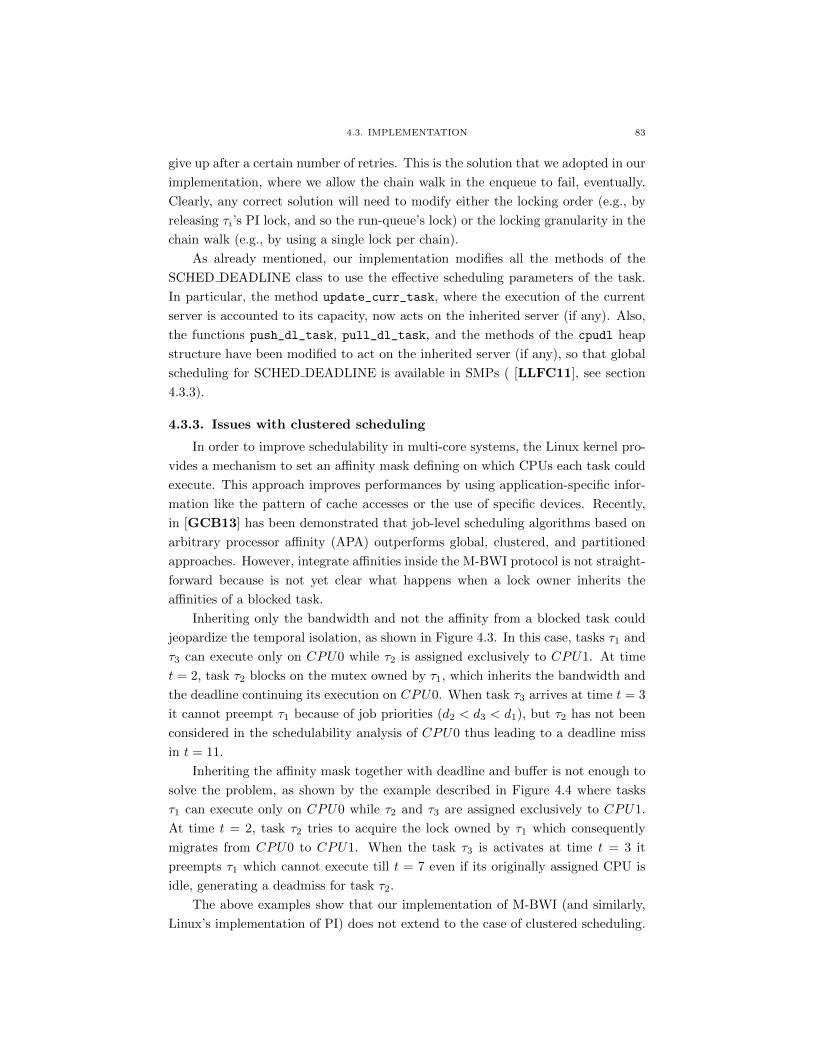
4.3. IMPLEMENTATION 83
give up after a certain number of retries. This is the solution that we adopted in our
implementation, where we allow the chain walk in the enqueue to fail, eventually.
Clearly, any correct solution will need to modify either the locking order (e.g., by
releasing τi’s PI lock, and so the run-queue’s lock) or the locking granularity in the
chain walk (e.g., by using a single lock per chain).
As already mentioned, our implementation modifies all the methods of the
SCHED DEADLINE class to use the effective scheduling parameters of the task.
In particular, the method update_curr_task, where the execution of the current
server is accounted to its capacity, now acts on the inherited server (if any). Also,
the functions push_dl_task, pull_dl_task, and the methods of the cpudl heap
structure have been modified to act on the inherited server (if any), so that global
scheduling for SCHED DEADLINE is available in SMPs ( [LLFC11], see section
4.3.3).
4.3.3. Issues with clustered scheduling
In order to improve schedulability in multi-core systems, the Linux kernel pro-
vides a mechanism to set an affinity mask defining on which CPUs each task could
execute. This approach improves performances by using application-specific infor-
mation like the pattern of cache accesses or the use of specific devices. Recently,
in [GCB13] has been demonstrated that job-level scheduling algorithms based on
arbitrary processor affinity (APA) outperforms global, clustered, and partitioned
approaches. However, integrate affinities inside the M-BWI protocol is not straight-
forward because is not yet clear what happens when a lock owner inherits the
affinities of a blocked task.
Inheriting only the bandwidth and not the affinity from a blocked task could
jeopardize the temporal isolation, as shown in Figure 4.3. In this case, tasks τ1 and
τ3 can execute only on CPU0 while τ2 is assigned exclusively to CPU1. At time
t = 2, task τ2 blocks on the mutex owned by τ1, which inherits the bandwidth and
the deadline continuing its execution on CPU0. When task τ3 arrives at time t = 3
it cannot preempt τ1 because of job priorities (d2 < d3 < d1), but τ2 has not been
considered in the schedulability analysis of CPU0 thus leading to a deadline miss
in t = 11.
Inheriting the affinity mask together with deadline and buffer is not enough to
solve the problem, as shown by the example described in Figure 4.4 where tasks
τ1 can execute only on CPU0 while τ2 and τ3 are assigned exclusively to CPU1.
At time t = 2, task τ2 tries to acquire the lock owned by τ1 which consequently
migrates from CPU0 to CPU1. When the task τ3 is activates at time t = 3 it
preempts τ1 which cannot execute till t = 7 even if its originally assigned CPU is
idle, generating a deadmiss for task τ2.
The above examples show that our implementation of M-BWI (and similarly,
Linux’s implementation of PI) does not extend to the case of clustered scheduling.
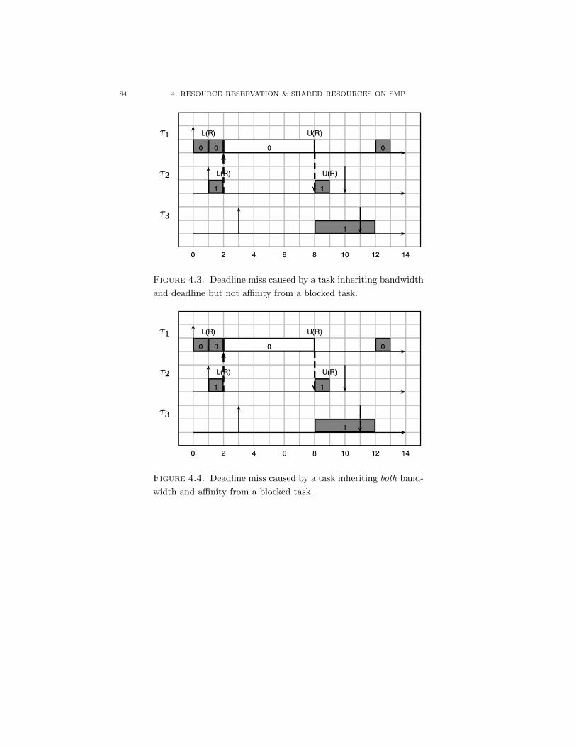
84 4. RESOURCE RESERVATION & SHARED RESOURCES ON SMP
Figure 4.3. Deadline miss caused by a task inheriting bandwidth
and deadline but not affinity from a blocked task.
Figure 4.4. Deadline miss caused by a task inheriting both band-
width and affinity from a blocked task.

4.4. EVALUATION 85
Brandenburg [Bra13], proposed the Migratory Priority Inheritance protocol for
clustered scheduling, and proved results of its optimality in terms of maximum PI-
blocking for Job-Level-Fixed-Priority scheduling (JLFP). Under migratory priority
inheritance, whenever a job J is not scheduled (but ready) and there exists a job
Ji waiting for J to release a resource such that Ji is eligible to be scheduled in its
assigned cluster, J migrates to Ji’s cluster (if necessary) and assumes Ji’s priority.
The idea is that jobs should inherit (both the priority and the affinity mask) only
when they “have to”. However it is not yet clear how to extend this idea to the
not-JLFP context, and how to implement it within the Linux kernel.
4.4. Evaluation
4.4.1. Experimental setup
We ran experiments on an Intel®Core2™ quad-core machine (Q6600) with
4GB of RAM and running at 2.4GHz.
Runtime validation consisted of executing two synthetic benchmarks. The first
implements a simple situation in which two tasks share a resource protected by
a mutex, and a third one, independent from the other two, is periodically acti-
vated to check if the inheritance mechanism works. The second executes a similar
configuration on an SMP system.
Runtime overheads were instead measured running another benchmark, called
(rt-app4). Using this application we simulated a real-time periodic load consisting
of multiple SCHED DEADLINE threads sharing resources protected by mutexes.
4.4.2. Runtime validation
We performed simple tests to validate the implementation. In the first test two
threads are run that operate on the same mutex (denoted as A). A third thread has
nothing to do with the first two, its only intent is to demonstrate that the M-BWI
mechanism (when enabled) works properly. All threads are restricted to execute
on the same CPU.
Figure 4.5 shows a visual representation5 of a run when M-BWI mechanism is
disabled. Threads τ1 and τ3 share a resource for which mutual exclusion is achieved
through the use of a mutex. Both threads are periodic with periods of 24ms and
72ms respectively (deadline are set equal to periods). τ1 executes entirely inside
the critical section for 8ms every period, τ3 has an execution time of 24ms of which
20ms are spent inside the critical section. τ2 has no critical section and executes for
8ms every 24ms. Thread τ3 is the first to be activated, after a while it acquires the
4https://github.com/gbagnoli/rt-app5Execution diagrams in this section are created through the KernelShark
(https://lwn.net/Articles/425583/) utility from execution traces extracted from the kernel
via ftrace (Documentation/trace/ftrace.txt).
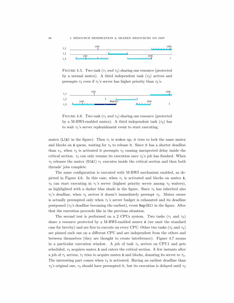
86 4. RESOURCE RESERVATION & SHARED RESOURCES ON SMP
t_1
t_2
t_3
L(A)
L(A)
U(A)
U(A)
Figure 4.5. Two task (τ1 and τ3) sharing one resource (protected
by a normal mutex). A third independent task (τ2) arrives and
preempts τ3 even if τ1’s server has higher priority than τ2’s.
t_1
t_2
t_3
L(A)
L(A)
U(A)
U(A)
S1
Rep(S1)
Figure 4.6. Two task (τ1 and τ3) sharing one resource (protected
by a M-BWI-enabled mutex). A third independent task (τ2) has
to wait τ1’s server replenishment event to start executing.
mutex (L(A) in the figure). Then τ1 is woken up, it tries to lock the same mutex
and blocks on A queue, waiting for τ3 to release it. Since it has a shorter deadline
than τ3, when τ2 is activated it preempts τ3 causing unexpected delay inside the
critical section. τ3 can only resume its execution once τ2’s job has finished. When
τ3 releases the mutex (U(A)) τ1 executes inside the critical section and then both
threads’ jobs complete.
The same configuration is executed with M-BWI mechanism enabled, as de-
picted in Figure 4.6. In this case, when τ1 is activated and blocks on mutex A,
τ3 can start executing in τ1’s server (highest priority server among τ3 waiters),
as highlighted with a darker blue shade in the figure. Since τ3 has inherited also
τ1’s deadline, when τ2 arrives it doesn’t immediately preempt τ3. Mutex owner
is actually preempted only when τ1’s server budget is exhausted and its deadline
postponed (τ2’s deadline becoming the earliest), event Rep(S1) in the figure. After
that the execution proceeds like in the previous situation.
The second test is performed on a 2 CPUs system. Two tasks (τ1 and τ3)
share a resource protected by a M-BWI-enabled mutex A (we omit the standard
case for brevity) and are free to execute on every CPU. Other two tasks (τ2 and τ4)
are pinned each one on a different CPU and are independent from the others and
between themselves (they are thought to create interference). Figure 4.7 zooms
in a particular execution window. A job of task τ3 arrives on CPU1 and gets
scheduled, τ3 acquires mutex A and enters the critical section. A few instants after
a job of τ1 arrives, τ1 tries to acquire mutex A and blocks, donating its server to τ3.
The interesting part comes when τ4 is activated. Having an earliest deadline than
τ3’s original one, τ4 should have preempted it, but its execution is delayed until τ3

4.4. EVALUATION 87
t_1
t_2
t_3
L(A)
t_4
L(A)
U(A)
U(A)
S1
Figure 4.7. System with two CPUs. Two task (τ1 and τ3) sharing
one resource (protected by a M-BWI-enabled mutex). Other two
independent tasks (τ2 and τ4) are pinned each one on a different
CPU.
releases mutex A and is consequently deboosted. After this instant of time execution
continues with original parameters. Without the M-BWI mechanism working τ3
would have been preempted inside the critical section by τ4, delaying τ1 execution.
4.4.3. Overheads measurements
We measured runtime overheads comparing execution of the same benchmark
with the M-BWI mechanism activated, with simple deadline inheritance, and against
the stock fixed priority Linux scheduler. Similarly to Brandenburg’s evaluation
[Bra13] evaluation, we launched on each core four tasks with periods 1ms, 25ms,
100ms, 1000ms and execution times of 0.1ms, 2ms, 15ms, 600ms. The one-
millisecond tasks did not access any shared resources. All other tasks shared the
same lock (one lock for each core) with an associated maximum critical section
length of 1ms, and each of their jobs acquired the lock once.
We ran the task set once using the stock Linux scheduler (SCHED FIFO with
priority inheritance enabled, called pi in what follows), once using the original
SCHED DEADLINE implementation (deadline inheritance, dl) and once with the
M-BWI mechanism enabled (bwi), for 60 seconds each. Although the same task
sets can be run with priority inheritance mechanisms turned off, we don’t report
results coming from that configurations here as they are hardy comparable to cases
when priority inheritance (or M-BWI) is enabled. In fact, execution paths inside
the kernel are completely different, and unrelated functions get called, thus making
the comparison of little interest for the present discussion.
Figure 4.8 shows the measurements of kernel functions, obtained using ftrace,
that could be ill-affected by the mechanism implementation:
a) schedule(), scheduler core, it decides which task to run next and per-
forms the context switch;
b) do futex(), sys futex() system call entry point;
c) enqueue task dl()/enqueue task rt(), enqueue a task, respectively, on
the dl or the rt runqueues;
d) rt mutex slowlock(), work required to acquire a mutex;

88 4. RESOURCE RESERVATION & SHARED RESOURCES ON SMP
a b c d e0
20
40
60
80
100
duratio
n (us)
bwidlpi
Figure 4.8. Kernel functions durations (in µs) from a run on a
real machine.
e) rt mutex slowunlock(), work required to release a mutex.
Results show that overheads of dl (yellow, oblique lines, boxes) and bwi (red boxes)
are comparable. Differences between bwi and pi (blue, small circles, boxes) mea-
surements remain in the same order of magnitude (even if bwi doubles pi in some
case). These differences can be ascribed to the slightly higher complexity of bwi
implementation, but also to the fact that tasks interactions can be modified by
scheduling the same task set using different scheduling policies (in this can have an
impact on runtime overheads).
We have then modified the previous example in order to create longer PI chains:
a new task with period 2000ms and execution time 700ms, and two more mutexes
were added to the above task set. Like in the previous example, there is a task
that does not use any resource; no task accesses more than two mutexes, but the
resulting PI chain can reach a depth of 4:
τ1 → R1 → τ2 → R2 → τ3 → R3 → τ4
We replicated this task set 3 times for a total of 15 tasks, due to bandwidth
constraint. The results displayed in Figure 4.9 show that the effect of the chain’s
depth contributes in an equivalent amount for the three implementations.

4.5. CONCLUSIONS 89
a b c d e0
20
40
60
80
100
duratio
n (us)
bwidlpi
Figure 4.9. Kernel functions durations (in µs) with nested criti-
cal sections, from a run on a real machine.
4.5. Conclusions
In this Chapter we presented an implementation of the M-BWI protocol in
the Linux kernel with the SCHED DEADLINE patch. We tried to be as adherent
as possible to the original implementation of the priority inheritance protocol in
Linux and to the SCHED DEADLINE patch by minimizing the number of mod-
ifications. The overhead of our implementation are comparable with the typical
overhead of SCHED DEADLINE and slightly larger than the overhead of the PI
with SCHED FIFO.
As future work, we are investigating the problems that we encountered when
trying to inherit the affinity mask of the lock-owner task. We believe that to
overcome such difficulties it is necessary to rethink the current implementation of
the SCHED DEADLINE patch, by introducing the concept of server as a separate
scheduling entity in the implementation.


CHAPTER 5
Conclusions
In this last chapter we briefly review the results achieved while working at this
thesis, suggesting possible directions for future work.
5.1. Summary of Results
The proposed goal of this thesis was to reduce the gap between real-time litera-
ture and industry, applying and implementing real-time scheduling mechanisms on
General Purpose Operating Systems. The focus has been on the Linux Operating
System in the context of modern Symmetric Multiprocessing computing platforms.
We started providing a general introduction, notation and definitions concern-
ing real-time systems in Chapter 1. We also detailed about differences and pecu-
liarities of Uniprocessor and Multiprocessors real-time sytems. We then concluded
the first Chapter with a taxonomy of different approaches in designign Operating
Systems and the predictability issues that may arise when such systems are not
originally thought for real-time system (as Linux is).
In Chapter 2, we described the structure of the Linux scheduler, and detailed
about our implementation of the global Earliest Deadline First scheduling algo-
rithm with hard and soft resource reservations (Constant Bandwidth Server). Such
implementation is now part of the Linux scheduler as a scheduling policy, and goes
under the name of SCHED DEADLINE. We also described several improvements
we achieved, over the original version of the scheduling policy, in performing ef-
ficient global scheduling decisions. Chapter 2 contains also a detailed description
PRAcTISE (Performance Analysis and Testing of real-time multicore Schedulers).
PRAcTISE is a framework we created that can be used to ease developing, testing
and debugging scheduling algorithms in user space, before implementing them in
the kernel.
We then used the work of Chapter 2 to perform, in Chapter 3, an experimen-
tal comparison of the performance of partitioned, clustered and global variants of
Rate Monotonic (RM) and Earliest Deadline First (EDF) scheduling algorithms
in the Linux Operating System. The purpose was to highlight where each of the
two algorithms excels or what are instead the problems that real-time application
developers may encounter in using such scheduling algorithms.
91

92 5. CONCLUSIONS
We then open the analysis to set of tasks that share resources. Given the fact
that resource reservation mechanisms are incompatible with classical resource access
protocols, we detailed about our implementation of the Multiprocessor Bandwidth
Inheritance protocol within SCHED DEADLINE. The protocol levers on the basic
idea of classical priority inheritance and extends it to work when interacting tasks
are scheduled using the Constant Bandwidth Server mechanism. It basically enables
donation of computing capacity between tasks accessing resources protected by
mutexes. We detail about technicalities of the implementation and we perform an
experimental evaluation of performance.
5.2. Future Work
There are several directions for future work and for refining and extending the
results presented in this thesis, as we detail next.
Hierarchical Scheduling
Hierarchical scheduling is an interesting methodology for design and deploying
real-time application, since it enables component-based design and analysis, and
supports temporal isolation among competing components. In this thesis we only
detailed about configurations where each task is assigned a single reservation (we
can also say that there is a 1-to-1 relashionship between tasks and reservations).
While this approach gives an high level of granularity in specifying real-time appli-
cation requirements, it can be not easy to translate requirements of an application
composed by several concurrent activities in single reservations for each of the com-
posing elements (or actually impossible, e.g., legacy applications of which we could
not know the internal design). It is therefore interesting to extend the presented
mechasims to provide hierarchical scheduling.
Resource Sharing
The meachanisms described in Chapter 4 are a basic extension of classical pri-
ority inheritance to systems that implement resource reservation mechanisms. As
we already stated, what we implemented is a first attemp in having the Multi-
processor Bandwidth Inheritance protocol working on top of our implementation
of Global EDF scheduling. While providing good runtime performace, our first
attemp is however quite far from a proper solution to the problem, both from a
theoretical and practical point of view (for example, as discussed in Section 4.3.2,
our implementation doesn’t consider busy-waiting of task that blocks on a mutex).
We are currently studying how to extend that implementation to actually remove
the need of busy-waiting, thus simplyfing practical implementation.
Reclaiming Mechanisms
The common practise in using resource reservation mechanisms, while guaran-
teeing applications performance, is to over-reserve resources based on worst-case

5.2. FUTURE WORK 93
resource usage estimates. This may lead to unnecessary wasting of system re-
sources, given that, especially for soft real-time systems, application requirements
are usually way below worst-case scenarios, and nothing terrible happens if some
deadlines are missed from time to time. Resource Reclaiming mechanisms allow
sharing of the over-allocation of resources. We are currently working on modify-
ing the SCHED DEADLINE scheduling policy to implement the GRUB (Greedy
Reclamation of Unused Bandwidth) scheduling algorithm. As the required modifi-
cations are quite simple and minimal, the benefits given by such an effort are likely
to be really promising.


Bibliography
[A. 11] A. Bastoni, B. B. Brandenburg, and J. H. Anderson. Is semi-partitioned sched-
uling practical? In Proc. 23rd Euromicro Conference on Real-Time Systems
(ECRTS 2011), pages 125–135, Porto, Portugal, July 2011.
[AB98] L. Abeni and G. Buttazzo. Integrating multimedia applications in hard real-
time systems. In Proc. IEEE Real-Time Systems Symposium, Madrid, Spain,
December 1998.
[AK13] L. Abeni and C. Kiraly. Running repeatable and controlled virtual routing
experiments. Software: Practice and Experience, pages n/a–n/a, 2013.
[AKLB13] L. Abeni, C. Kiraly, N. Li, and A. Bianco. Tuning KVM to Enhance Virtual
Routing Performance. In Proceedings of the IEEE ICC’2013, pages 2396–2401.
IEEE, 2013.
[BA07] B. Brandenburg and J. Anderson. Feather-trace: A lightweight event tracing
toolkit. In Proceedings of the third international workshop on operating systems
platforms for embedded real-time applications, pages 19–28, 2007.
[BA09] B. B. Brandenburg and J. H. Anderson. On the implementation of global real-
time schedulers. In Proceedings of the 30th IEEE Real-Time Systems Sympo-
sium, RTSS ’09, pages 214–224, Washington, DC, USA, 2009. IEEE Computer
Society.
[Bak91] T. P. Baker. Stack-based scheduling for realtime processes. Real-Time Systems,
3(1):67–99, April 1991.
[Bak06] T. P. Baker. A comparison of global and partitioned EDF schedulability tests
for multiprocessors. In Proceeding of the International Conference on Real-
Time and Network Systems, Poitiers, France, 2006.
[BB10] M. Bertogna and S. Baruah. Tests for global EDF schedulability analysis. Jour-
nal of Systems Architecture, 57:487–497, September 2010.
[BB11] M. Bertogna and S. Baruah. Tests for global EDF schedulability analysis. Jour-
nal of Systems Architecture, 57(5):487 – 497, 2011. Special Issue on Multipro-
cessor Real-time Scheduling.
[BBA10a] A. Bastoni, B. Brandenburg, and J. Anderson. An empirical comparison of
global, partitioned, and clustered multiprocessor edf schedulers. In Real-Time
Systems Symposium (RTSS), 2010 IEEE 31st, pages 14–24, 30 2010-dec. 3
2010.
[BBA10b] A. Bastoni, B. B. Brandenburg, and J. H. Anderson. Cache-related preemp-
tion and migration delays: Empirical approximation and impact on schedu-
lability. In Proc. 6th International Workshop on Operating Systems Platforms
95

96 BIBLIOGRAPHY
for Embedded Real-Time Applications (OSPERT 2010), pages 33–44, Brussels,
Belgium, July 2010.
[BBB03] E. Bini, G. C. Buttazzo, and G. M. Buttazzo. Rate monotonic analysis: the
hyperbolic bound. Computers, IEEE Transactions on, 52(7):933–942, 2003.
[BC07] M. Bertogna and M. Cirinei. Response-time analysis for globally scheduled
symmetric multiprocessor platforms. In Real-Time Systems Symposium, 2007.
RTSS 2007. 28th IEEE International, pages 149–160, dec. 2007.
[BCA08] B. Brandenburg, J. Calandrino, and J. Anderson. On the scalability of real-
time scheduling algorithms on multicore platforms: A case study. In Real-Time
Systems Symposium, 2008, pages 157–169, 30 2008-dec. 3 2008.
[BLAC06] G. C. Buttazzo, G. Lipari, L. Abeni, and M. Caccamo. Soft Real-Time Systems:
Predictability vs. Efficiency: Predictability vs. Efficiency. Springer, 2006.
[Bra13] B. B. Brandenburg. A fully preemptive multiprocessor semaphore protocol
for latency-sensitive real-time applications. In Proceedings of 25th Euromicro
Conference on Real-Time Systems (ECRTS 2013), pages 292–302, July 2013.
[But05] G. Buttazzo. Rate Monotonic vs. EDF: Judgment Day. Real-Time Systems,
29(1), 2005.
[But11] G. C. Buttazzo. Hard real-time computing systems: predictable scheduling al-
gorithms and applications, volume 24. Springer, 2011.
[CAB07] J. M. Calandrino, J. H. Anderson, and D. P. Baumberger. A hybrid real-time
scheduling approach for large-scale multicore platforms. In Real-Time Systems,
2007. ECRTS’07. 19th Euromicro Conference on, pages 247–258. IEEE, 2007.
[CBL+08] J. M. Calandrino, D. P. Baumberger, T. Li, J. C. Young, and S. Hahn. Lin-
sched: The linux scheduler simulator. In ISCA PDCCS, pages 171–176, 2008.
[CGKS05] D. Chandra, F. Guo, S. Kim, and Y. Solihin. Predicting inter-thread cache
contention on a chip multi-processor architecture. In High-Performance Com-
puter Architecture, 2005. HPCA-11. 11th International Symposium on, pages
340 – 351, feb. 2005.
[CLB+06] J. M. Calandrino, H. Leontyev, A. Block, U. C. Devi, and J. H. Anderson.
LITMUS-RT: A testbed for empirically comparing real-time multiprocessor
schedulers. In Proceedings of the 27th IEEE International Real-Time Systems
Symposium, pages 111–126, Washington, DC, USA, 2006. IEEE Computer
Society.
[DA08] U. Devi and J. Anderson. Tardiness bounds under global edf scheduling ona-
multiprocessor. Real-Time Systems, 38(2):133–189, 2008.
[DCC07] F. M. David, J. C. Carlyle, and R. H. Campbell. Context switch overheads
for linux on arm platforms. In Proc. of the 2007 Workshop on Experimental
Computer Science, San Diego, USA, June 2007.
[DD06] M. Desnoyers and M. R. Dagenais. The lttng tracer: A low impact performance
and behavior monitor for GNU/Linux. In Proc. Ottawa Linux Symposium (OLS
2006), pages 209–224, July 2006.
[Den68] P. J. Denning. The working set model for program behavior. Communications
of the ACM, 11(5):323–333, May 1968.
BIBLIOGRAPHY 97
[Des09] M. Desnoyers. Lttng, filling the gap between kernel instrumentation and a
widely usable kernel tracer. Linux Foundation Collaboration Summit, April
2009.
[DL78] S. K. Dhall and C. Liu. On a real-time scheduling problem. Operations Re-
search, 26(1):127–140, 1978.
[DM03] L. Dozio and P. Mantegazza. Real time distributed control systems using
rtai. In 2008 11th IEEE International Symposium on Object and Component-
Oriented Real-Time Distributed Computing (ISORC), pages 11–11. IEEE Com-
puter Society, 2003.
[Edg13] J. Edge. Elc: Spacex lessons learned, 2013.
[ESD10] P. Emberson, R. Stafford, and R. I. Davis. Techniques for the synthesis of
multiprocessor tasksets. In Proceedings of the 1st International Workshop on
Analysis Tools and Methodologies for Embedded and Real-time Systems (WA-
TERS 2010), pages 6–11, Brussels, Belgium, July 2010.
[FCTS09] D. Faggioli, F. Checconi, M. Trimarchi, and C. Scordino. An EDF scheduling
class for the Linux kernel. In Proceedings of the 11th Real-Time Linux Work-
shop, Dresden, Germany, September 2009.
[FLC12] D. Faggioli, G. Lipari, and T. Cucinotta. Analysis and implementation of the
multiprocessor bandwidth inheritance protocol. Real-Time Systems, 48:789–
825, 2012.
[GCB13] A. Gujarati, F. Cerquerira, and B. B. Brandenburg. Schedulability analysis of
the linux push and pull scheduler with arbitrary processor affinities. In Pro-
ceedings of the 25th Euromicro conference on Real-time systems, ECRTS13,
pages 69–79. IEEE Computer Society, 2013.
[GS88] J. B. Goodenough and L. Sha. The Priority Ceiling Protocol: A Method
for Minimizing the Blocking of High-Priority Ada Tasks. Technical Report
CMU/SEI-88-SR-4, Carnegie-Mellon University, March 1988.
[HP09] D. Hardy and I. Puaut. Estimation of cache related migration delays for multi-
core processors with shared instruction caches. In Proc. of the 17th Interna-
tional Conference on Real-Time and Network Systems (RTNS 2009), pages
45–54, Paris, France, October 2009.
[IEE04] IEEE. Information Technology - Portable Operating System Interface - Part
1: System Application Program Interface Amendment: Additional Realtime
Extensions. 2004.
[KKL+07] A. Kivity, Y. Kamay, D. Laor, U. Lublin, and A. Liguori. KVM: the Linux
Virtual Machine Monitor. In Proceedings of the Linux Symposium, Ottawa,
Ontario, Canada, 2007.
[LDS07] C. Li, C. Ding, and K. Shen. Quantifying the cost of context switch. In Pro-
ceedings of the 2007 workshop on Experimental computer science, ExpCS ’07,
New York, NY, USA, 2007. ACM.
[LFCL12] J. Lelli, D. Faggioli, T. Cucinotta, and G. Lipari. An experimental comparison
of different real-time schedulers on multicore systems. Journal of Systems and
Software, 85(10):2405–2416, 2012.

98 BIBLIOGRAPHY
[LIT] Linux Testbed for Multiprocessor Scheduling in Real-Time Systems
(LITMUSRT ). http://www.cs.unc.edu/ anderson/litmus-rt/.
[LL73] C. L. Liu and J. Layland. Scheduling alghorithms for multiprogramming in a
hard real-time environment. Journal of the ACM, 20(1), 1973.
[LLA01] G. Lamastra, G. Lipari, and L. Abeni. A bandwidth inheritance algorithm for
real-time task synchronization in open systems. In Real-Time Systems Sym-
posium, 2001. (RTSS 2001). Proceedings. 22nd IEEE, pages 151 – 160, dec.
2001.
[LLA04] G. Lipari, G. Lamastra, and L. Abeni. Task synchronization in reservation-
based real-time systems. IEEE Trans. Computers, 53(12):1591–1601, 2004.
[LLFC11] J. Lelli, G. Lipari, D. Faggioli, and T. Cucinotta. An efficient and scalable im-
plementation of global EDF in Linux. In Proceedings of the 7th Annual Work-
shop on Operating Systems Platforms for Embedded Real-Time applications
(OSPERT 2011), Porto, Portugal, 2011.
[MB91] J. C. Mogul and A. Borg. The effect of context switches on cache performance.
ACM SIGPLAN Notices, 26(4):75–84, 1991.
[MCF10] A. Masrur, S. Chakraborty, and G. Faerber. Constant-time admission control
for partitioned EDF. In Real-Time Systems (ECRTS), 2010 22nd Euromicro
Conference on, pages 34 –43, July 2010.
[Mel10] A. Melo. The new linux ’perf’ tools. In 17 International Linux System Tech-
nology Conference (Linux Kongress), Georg Simon Ohm University Nuremberg
(Germany), September 21-24 2010.
[Pao10] G. Paoloni. How to benchmark code execution times on Intel IA-32 and IA-64
Instruction Set Architectures. Intel White Paper, September 2010.
[Ros09] S. Rostedt. The world of ftrace. Linux Foundation Collaboration Summit, April
2009.
[SA04] J. Starner and L. Asplund. Measuring the cache interference cost in preemptive
real-time systems. ACM SIGPLAN Notices, 39(7):146–154, 2004.
[SK11] G. L. Stavrinides and H. D. Karatza. Scheduling multiple task graphs in het-
erogeneous distributed real-time systems by exploiting schedule holes with bin
packing techniques. Simulation Modelling Practice and Theory, 19(1):540 –
552, 2011. Modeling and Performance Analysis of Networking and Collabora-
tive Systems.
[SRL90] L. Sha, R. Rajkumar, and J. P. Lehoczky. Priority inheritance protocols:
An approach to real-time synchronization. IEEE Transactions on Computers,
39(9), September 1990.
[Sta14] W. Stallings. Operating Systems: Internals and Design Principles, 8/E. Pren-
tice Hall, 2014.
[TLL+11] X. Tang, K. Li, G. Liao, K. Fang, and F. Wu. A stochastic scheduling algorithm
for precedence constrained tasks on grid. Future Generation Computer Systems,
27(8):1083 – 1091, 2011.
[Tsa07] D. Tsafrir. The context-switch overhead inflicted by hardware interrupts. In
Proc. of the 2007 Workshop on Experimental Computer Science, San Diego,
USA, 6 2007.

BIBLIOGRAPHY 99
[YB97] V. Yodaiken and M. Barabanov. Real-time linux applications and design. In
Proceedings of the Linux Applications Development and Deployment Confer-
ence (USELINUX), 1997.
[YZ08] J. Yan and W. Zhang. WCET analysis for multi-core processors with shared l2
instruction caches. In Proceedings of the 2008 IEEE Real-Time and Embedded
Technology and Applications Symposium, pages 80–89, Washington, DC, USA,
2008. IEEE Computer Society.