Multiproduct Aggregate Production Planning with Flexible

Requirement Profile

A Case Study

Taylor Ballard, Dr. Ertunga Ozelkan

University of North Carolina at Charlotte

Table of Contents

Abstract ........................................................................................................................................... 1

Introduction ..................................................................................................................................... 2

Literature Review............................................................................................................................ 2

Methodology ................................................................................................................................... 5

Model Formulation ..................................................................................................................... 6

Remark I.................................................................................................................................... 11

Performance Comparison.......................................................................................................... 12

Application and Case Study .......................................................................................................... 12

The Company ............................................................................................................................ 12

Application ................................................................................................................................ 14

Challenges ................................................................................................................................. 15

Results ........................................................................................................................................... 17

Summary and Conclusion ............................................................................................................. 18

References ..................................................................................................................................... 20

Appendix I: Figures ...................................................................................................................... 23

Appendix 2: Tables ....................................................................................................................... 27

1

Abstract

The purpose of this study is to apply aggregate production planning with flexible requirement

profile (FRP-APP) to a real, multiproduct, production planning problem. FRP-APP has been

proposed and proven successful on several experimental data types, but it has not yet been

deployed in a real production environment. FRP-APP model design is focused on trading off

between the traditional cost objective and a new plan stability objective to minimize rapid plan

fluctuations in case of demand uncertainties to yield stable yet cost efficient production plans.

The model is claimed to be more realistic and flexible than other traditional APP models for

production planning. The proposed case study will deploy this technique in a production

environment in the telecommunications industry and assess its performance in terms of cost and

stability while adding a multiproduct aspect that has not been explored previously. The study

includes notations between a production environment that incorporates a work-in-progress type

of inventory and the same environment without it to evaluate how this effects the overall stability

and cost of the facility

2

Introduction

Within the production environment, reducing costs of operation is the top priority and generally

achievable through appropriate planning procedures. An additional interest of a manufacturing

company includes tracking, planning for, and limiting the effects of nervousness and uncertainty

in regard to the production environment. This uncertainty can come from the demand forecast,

the internal or external supply process, general logistics and globalization of the market, and

other areas that are not concrete within the planning process. These uncertainties can create

nervousness within the company that in turn cause frequent changes in production plans that

potentially add unnecessary expenditures and overly stressed environments.

Traditional methods that have been used to stabilize production planning, despite the

uncertainties, may not allow for the required flexibility a plant needs to meet their demand. One

method of completing this stability in the planning process is to use aggregate production

planning (APP). APP is a method of determining quantities for production, workforce, and

inventory levels a company will need over a selected production horizon. By adding flexible

requirement profiles (FRP) to the aggregate production plan, manufacturing environments can

deal with the uncertainty in their planning parameters. It has been shown that FRP can reduce

instability and nervousness by limiting plan fluctuations to a level the company finds acceptable

while also meeting demand.

At the University of North Carolina at Charlotte, research has been conducted to develop several

FRP based APP models that were applied to industry-based data sets published in literature.

These methodologies have allowed for a closer look at the tradeoffs between cost and stability

when managing uncertainty within the production plan. The research proposed here includes

conducting a case study application for a telecommunication company of the model and methods

developed within these previous studies and adds a multiproduct aspect to the analysis.

Objectives of this study include:

• Build a multiproduct aggregate production planning model with flexible requirement

profile that will dictate production quantities for a company within the

telecommunications industry on a weekly basis to meet demand trends and safety stock

requirements

• Include the ability for products within model that utilize the same resources but have

individualized cost, demand, limitations of production, and quantity constraints

• Introduce the interactions between different phases of production, various workforce

teams, and dual-leveled inventory constraints

• Validate the model performance with a traditional aggregate production planning model

and the company’s current operation standards.

• Evaluate how different flex limits and workforce parameters effect actual cost and plan

variability for this application

Literature Review

Aggregate Production Planning has been used to allocate resources and respond to changing

demand levels while minimizing the overall cost within a finite time horizon. These costs are

adjusted through changing production, workforce, inventory holding, backorder potential, while

3

meeting the markets demand of products being offered. Looking into future realized and

expected demand of products and the resources available, aggregate production planning

provides a way to optimize the manufacturing environment and create a workable solution that

affords the company the ability to meet their goals.

Mathematical programming of models for aggregate production planning have been completed

in a few ways since its inception. Starting with (Holt, Modigliani, & Herbert, A Linear Decision

Rule for Production and Employment Scheduling, 1955), who initialized the research with

determining how linear decision rules could be applied to determine optimal production and

workforce levels while minimizing costs. Holt, and team, set up the base work for all aggregate

production models since. Traditional models have included a minimization of costs or a

maximization of profits with each period having decisions made based on satisfying constraints

at an aggregate level. While a range of approaches have been built from this initial work to solve

for optimized solutions within the production environment using aggregate production planning,

the two that have often been accepted and used are linear programming and mixed-integer linear

programming.

Mixed-integer linear programming is an optimization problem with a linear objective function,

linear constraints, and some integer variables. The traditional way of applying this method to

aggregate production planning problems includes having discrete time periods within the

planning horizon where each time period has constraints to satisfying when building the

optimized result. For applications like this, where the goal is to minimize the costs incurred

based on available resources and known or estimated demand, a single objective is typically

used. This application is additionally suitable for problems where there is a goal to minimize the

materials used. Like, (Demirel E. , 2014), this application will be based on a linear programming

model. However, it will be a multiproduct application whereas (Demirel E. , 2014) was focused

on single product application.

To allow the capacity to investigate future plans and include new information in a meaningful

way, a rolling horizon can be paired with aggregate production planning. Longer planning

horizons can increase visibility to the individual building the model, but they are less accurate,

and theory suggests forecasts too far out have no effect on current period decisions. (Wagner &

Whitin, 1958) (Baker & Peterson, An Analytic Framework for Evaluating Rolling Schedules,

1979). One of the first studies to look at the effectiveness of rolling horizon models within

production was (Baker, An Experimental Study of the Effectiveness of Rolling Schedules in

Production Planning, 1977). They found that rolling schedules were efficient, but demand pattern

and length of planning horizon had an impact on the effectiveness of this method being applied.

Another study, (McClain & Thomas, 1977), found that the length of the rolling horizon can

negatively impact the cost performance of the model

While having a long rolling horizon can impede the performance of a model, having to

frequently run the planning model due to a low or no rolling horizon can have effects on its

performance as well. A higher frequency can assist in using more current information and

meeting demand as it appears to create a more accurate model. This would also assist in reducing

the effect of uncertainty of the plan. Conversely, running the plan too frequently to continuously

add new information as it is available can increase the frequency of changes in the plan which

will increase instability within the manufacturing environment and cause stress within the

production environment. (Chung & Krajewski, 2007) suggests that having less frequency

4

planning does not have a significant change in projected costs when compared to rolling one

period at a time. (Lin, Krajewski, Leong, & Benton, 1994) shows that the ability for replanning

frequency to be high and have good results for the company, depends more on product cost

structure, lead time, and the length of the frozen interval.

In addition to reducing costs, maximizing profits, and looking further into the future, another

main characteristic of aggregate production plan application is that it can be used to reduce

nervousness within the plant. Nervousness can be caused by excessive plan changes due to

uncertainty and variability in demand causing a lack of confidence in the planning system (Kok

& Inderfurth, 1997). Variations in demand can cause information distortion up the supply chain

and create issues like higher costs/inventories/backorders and inefficient use of resources

referred to as the bullwhip effect. (Lee, Padmanabhan, & Whang, 1997). Additionally, frequent

changes can cause issues in scheduling and capacity utilizations (Inman & Gonsalvez, 1997). To

suppress that nervousness, plans can use things like production smoothness and plant stability

measures. Production smoothness limits the variability of production output via changes over the

production horizon and is achieved through advanced production and inventory accumulation

when inventory carrying costs are low or when businesses can alter the demand pattern through

pricing and promotions. (Kamien & Li, 1990) Plan stability refers to the variance of planned

revision between the planned production and the actual production that occurs from one period to

another during rolling horizon. Even when these options lead to less optimal cost solutions, it is a

general agreement that increasing the stability of a plan is important for the successful

application of that plan and the business.

Another method to cope with demand variability includes implementing safety stocks and lead

times within the production environment. Safety stock covers any demand swings by absorbing

changes at the overhead level and reduces instability at the lower level. High safety stocks can

improve stability but can present a high inventory holding cost which is dependent on the

application. According to (Yano & Carlson, 1987), using a safety stock is a viable option within

a production plan to reduce negative impacts of changing demand if the frequency of

rescheduling is low. (Sridharan & LaForge, The Impact of Safety Stock on Schedule Instability,

Cost and Service, 1989) suggests that having a safety stock below some ideal level can eliminate

instability while also reducing costs. However, there could be additional nervousness if safety

stock levels are incorrectly determined and out of the scope of the company to realistically keep.

(Buzacott & Shanthikumar, 1994) presents the idea that safety stock should be used over safety

lead time when the forecast accuracy is low because of the input changes from customers.

A more effective way to reduce nervousness within a rolling horizon model is to freeze

production schedules within the horizon. (Kadipasaoglu & Sridharan, 1995) explored three

strategies under demand uncertainty and found that freezing horizon was the most effective

method within their application to reduce nervousness. However, (Sridharan, Berry, &

Udayabhanu, Freezing the Master Production Schedule Under Rolling Planning Horizons, 1987)

found that costs can increase with the frozen horizon method when it is applied to over 50% of

the planning horizon. It is important to determine how much stability the application will require

vs how much more cost it can accrue before being nonbeneficial. According to (Zhao & Lee,

1993), costs can also increase with frozen horizons if the demand are too uncertain at the time of

planning. The frozen horizon method has also been proven to be not cost effective in industries

with high optioned products like the automotive industry by (Meixell, 2005).

5

One method to implement these frozen horizons, if applicable, is through rate-based planning

and flexible requirement planning, introduced by (Srinivasan, 2004), where you can add time

fences over a certain period of time to act as a frozen horizon. Time fences are defined as being

the bounds allowed for change to total demand within a time period and were introduced by

(Costanza, 1996). Up until (Demirel E. , 2014), (Demirel, Ozelkan, & Lim, 2018), and

(Torabzadeh & Ozelkan, 2016) there had been no research completed to investigate the

usefulness and application of flexible requirement profiles with aggregate production planning.

This research expands on the application of flexible requirement profiles and includes the

combined use of safety stock and frozen horizons to limit nervousness while adding the

multiproduct aspect into aggregate production planning through a case study from the

telecommunications industry.

Methodology

The case study will show a multiproduct flexible requirement profile aggregate production plan

(FRP-APP) for use within the telecommunications industry. Some variables and interactions

from the FRP-APP models proposed by (Torabzadeh & Ozelkan, 2016) and (Demirel, Ozelkan,

& Lim, 2018) have been adjusted, removed, or otherwise transitioned, but the concepts are

applied the same. The multiproduct aspect of the model is newly proposed as well as the

combination of both molding and human production constraints.

Removed parameters that some use cases will need to include are inventory holding cost per

period and back order cost per period. These values are not applicable here due to the company

dynamics being modeled. Inventory holding cost for this company is considered to be zero as a

result of how items are stored and the size of the products. Furthermore, the company has an

internal system that stops back orders from occurring. This is a two-fold prevention within the

sales team paired with a minimum required inventory covering their expectant monthly orders at

least twice over. Through this logic, the planned ahead backorder variable has also been removed

from the model.

The molding constraints and multi-product aspect of the formulation are directly correlated to the

use case. Because this use case is for one molding operation that is reconfigured between

multiple products as demand requires, rather than a single product line, an index has been added

to separate the product lines within the common molding operation. Additionally, products

manufactured here go through a 2-step process where they are first molded at a machine and then

post-processed by a member of either the regular or subcontract workforce before being entered

into inventory. From this interaction between the machined parts and human workforce, this

model contains both molding and workforce constraints on resources to meet demand.

Further variables that were altered or excluded from the (Torabzadeh & Ozelkan, 2016) model

are the workforce, hiring, and layoff levels of the company. For this use case, it is not desirable

for the model to define these values each period, or at all. Workforce levels are steady and range

between two teams to complete production tasks: the internal or “regular” workforce, and the

subcontracted workforce through a third party. Internally, the company has a low turnover rate,

with layoffs only having been formally completed within the production team once in the

company’s 28-year history. Within the internal workforce, the workforce level is defined in two

ways, the members who are scheduled to the post-processing task, which interacts with the

6

model’s results, and the total workforce, which acts as a constraint on the model. Having the

regular workforce defined in this way allows a realistic expectation of both the capacity of

regular production and sets a minimum number of molded parts to meet internal operation. This

minimum is necessary and used when some portion of the regular workforce is not needed

elsewhere in the manufacturing plant to keep them productive waiting between assignments. The

company does not control the hiring or layoff of the subcontracted workforce but does keep a

routine check-in with the workforce levels through approvals on work, or parts, available. Most

post-processing operations go through the subcontracted workforce because they are cheaper and

more efficient than the internal workforce at this task.

A mathematical model used is summarized below.

Model Formulation

Indices:

𝑗: index for planning horizon, 𝑗 = 0, … , 𝐽

𝑡: index for rolling horizon, 𝑡 = 1, … , 𝑇

𝑘: index for product line, 𝑘 = 1, … , 𝐾

Parameters:

𝐽: Total number of periods in the planning horizon

T: Total number of iterations

K: Total number of products/last product included

𝑐𝑘𝑅: labor cost of regular worker per unit in product line k

𝑐𝑘𝑂: labor cost of an overtime worker per unit in product line k

𝑐𝑘𝑆: labor cost of a subcontract worker per unit in product line k

𝑐𝑘𝑃: unit production cost per period in product line k

𝑈𝑅: maximum number of units produced per regular worker per period

𝑈𝑂: maximum number of units produced with overtime per worker per period

𝑈𝑆maximum number of units produced with subcontract worker per period

𝑈𝑘𝑀: maximum number of units produced by a mold per period for product line k

𝑊𝑗𝑅𝑇: j-step ahead planned regular true/scheduled workforce

𝑊𝑗𝑅𝐴: j-step ahead planned regular available workforce

𝑊𝑗𝑆: j-step ahead planned subcontract workforce

𝑑𝑡,𝑗,𝑘: j-step ahead estimated demand in planning iteration t and product line k

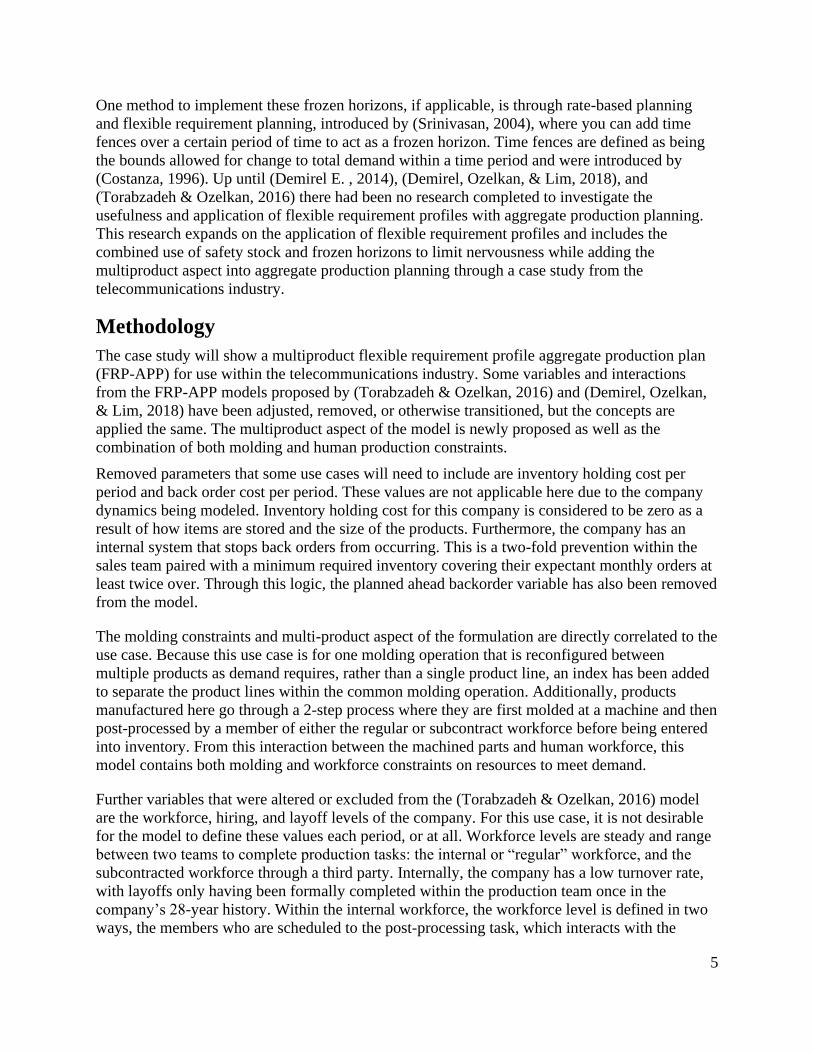
𝐼𝑡,𝑗,𝑘𝑚𝑖𝑛: j-step ahead safety stock planned for each period in planning iteration t and product line k

7

𝐼𝑡,𝑗,𝑘𝑚𝑎𝑥 j-step ahead maximum inventory planned for each period in planning iteration t and

product line k

𝑊𝐼𝑃𝑡,𝑗,𝑘𝑚𝑖𝑛: j-step ahead planned minimum WIP in planning iteration t and product line k

𝑊𝐼𝑃𝑡,𝑗,𝑘𝑚𝑎𝑥: j-step ahead planned maximum WIP in planning iteration t and product line k

𝑊𝑡,𝑗,𝑘𝑀 : j-step ahead planned molds available per period in planning iteration t and product line k

𝑀𝑡,𝑗𝑀𝑎𝑥: j-step ahead planned maximum molds in planning iteration t

𝐹𝑗: j-step ahead planned flex-limit

𝐿𝐵𝑅𝑡,𝑗,𝑘: j-step ahead lower bound on planned regular production calculated for planning

iteration t

𝑈𝐵𝑅𝑡,𝑗,𝑘: j-step ahead upper bound on planning regular production calculated for planning

iteration t

𝐿𝐵𝑆𝑡,𝑗,𝑘: j-step ahead lower bound on planned subcontract production calculated for planning

iteration t

𝑈𝐵𝑆𝑡,𝑗,𝑘: j-step ahead upper bound on planning subcontract production calculated for planning

iteration t

𝐿𝐵𝑂𝑡,𝑗,𝑘: j-step ahead lower bound on planned overtime production calculated for planning

iteration t

𝑈𝐵𝑂𝑡,𝑗,𝑘: j-step ahead upper bound on planning overtime production calculated for planning

iteration t

Variables:

𝑅𝑡,𝑗,𝑘: j-step ahead planned regular production level in planning iteration t and product line k

𝑂𝑡,𝑗,𝑘: j-step ahead planned overtime production level in planning iteration t and product line k

𝑆𝑡,𝑗,𝑘: j-step ahead planned subcontract production level in planning iteration t and product line k

𝐼𝑡,𝑗,𝑘: j-step ahead planned inventory level in planning iteration t and product line k

𝑀𝑡,𝑗,𝑘: j-step ahead planned number of molds to use in planning iteration t and product line k

𝑊𝐼𝑃𝑡,𝑗,𝑘: j-step ahead planned “work in-progress” units in planning iteration t and product line k

MILP formulation

Minimize: (1)

∑ ∑ [𝑐𝑘𝑅 ∙ 𝑅𝑡,𝑗,𝑘 + 𝑐𝑘

𝑂 ∙ 𝑂𝑡,𝑗,𝑘 + 𝑐𝑘𝑆 ∙ 𝑆𝑡,𝑗.𝑘 + 𝑐𝑘

𝑃 ∙ 𝑀𝑡,𝑗,𝑘 ∙ 𝑈𝑘𝑀]𝐽

𝑗=0𝐾𝑘=1

8

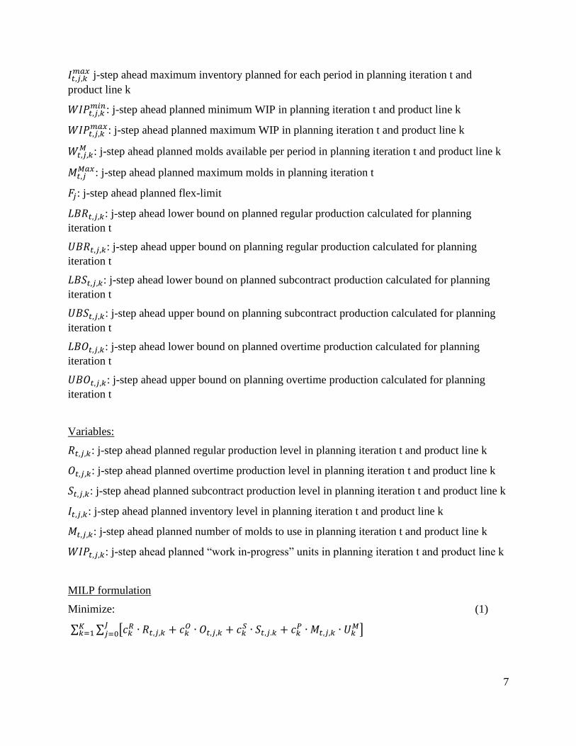
Subject To

Initial Inventory: 𝐼𝑡,0,𝑘 = 𝐼𝑡−1,0,𝑘 + 𝑅𝑡,𝑗,𝑘 + 𝑂𝑡,𝑗,𝑘 + 𝑆𝑡,𝑗,𝑘 − 𝑑𝑡,2,𝑘 (2)

Inventory: 𝐼𝑡,𝑗,𝑘 = 𝐼𝑡,𝑗−1,𝑘 + 𝑅𝑡,𝑗,𝑘 + 𝑂𝑡,𝑗,𝑘 + 𝑆𝑡,𝑗,𝑘 − 𝑑𝑡,𝑗+2,𝑘 (3)

Minimum Inventory: 𝐼𝑡,𝑗,𝑘 ≥ 𝐼𝑡,𝑗,𝑘𝑚𝑖𝑛 (4)

Maximum Inventory: 𝐼𝑡,𝑗,𝑘 ≤ 𝐼𝑡,𝑗,𝑘𝑚𝑎𝑥 (5)

Initial Work In Progress: 𝑊𝐼𝑃𝑡,0,𝑘 = 𝑈𝑘𝑀 ∙ 𝑀𝑡,0,𝑘 − 𝑅𝑡,0,𝑘 − 𝑂𝑡,0,𝑘 − 𝑆𝑡,0,𝑘 + 𝑊𝐼𝑃𝑡−1,0,𝑘 (6)

Work In Progress: 𝑊𝐼𝑃𝑡,𝑗,𝑘 = 𝑈𝑘𝑀 ∙ 𝑀𝑡,𝑗,𝑘 − 𝑅𝑡,𝑗,𝑘 − 𝑂𝑡,𝑗,𝑘 − 𝑆𝑡,𝑗,𝑘 + 𝑊𝐼𝑃𝑡,𝑗−1,𝑘 (7)

Minimum WIP: 𝑊𝐼𝑃𝑡,𝑗,𝑘 ≥ 𝑊𝐼𝑃𝑡,𝑗,𝑘𝑚𝑖𝑛 (8)

Capacity WIP: 𝑊𝐼𝑃𝑡,𝑗,𝑘 ≤ 𝑊𝐼𝑃𝑡,𝑗,𝑘𝑚𝑎𝑥 (9)

Minimum regular: ∑ 𝑅𝑡,𝑗,𝑘𝐾𝑘=1 ≥ 𝑈𝑅 ∙ 𝑊𝑗

𝑅𝑇 (10)

Capacity Regular: ∑ 𝑅𝑡,𝑗,𝑘𝐾𝑘=1 ≤ 𝑈𝑅 ∙ 𝑊𝑗

𝑅𝐴 (11)

Capacity Subcontract: ∑ 𝑆𝑡,𝑗,𝑘𝐾𝑘=1 ≤ 𝑈𝑆 ∙ 𝑊𝑗

𝑆 (12)

Capacity Overtime: ∑ 𝑂𝑡,𝑗,𝑘𝐾𝑘=1 ≤ 𝑈𝑂 ∙ 𝑊𝑗

𝑆 (13)

Max Molds: ∑ 𝑀𝑡,𝑗,𝑘𝐾𝑘=1 ≤ 𝑀𝑡,𝑗

𝑀𝑎𝑥 (14)

Molds Available: 𝑀𝑡,𝑗,𝑘 ≤ 𝑊𝑘𝑀 (15)

Mold Production Capacity: 𝑅𝑡,𝑗,𝑘+𝑂𝑡,𝑗,𝑘+𝑆𝑡,𝑗,𝑘

𝑈𝑘𝑀 ≤ 𝑊𝑘

𝑀 (16)

Even Number of Molds: 𝑀𝑡,𝑗,𝑘 = 2 ∗ ⌈

𝑅𝑡,𝑗,𝑘+𝑂𝑡,𝑗,𝑘+𝑆𝑡,𝑗,𝑘

𝑈𝑘𝑀

2⌉ (17)

FRP Regular: 𝐿𝐵𝑅𝑡,𝑗,𝑘 ≤ 𝑅𝑡,𝑗,𝑘 ≤ 𝑈𝐵𝑅𝑡,𝑗,𝑘 (18)

FRP Subcontract: 𝐿𝐵𝑆𝑡,𝑗,𝑘 ≤ 𝑆𝑡,𝑗,𝑘 ≤ 𝑈𝐵𝑆𝑡,𝑗,𝑘 (19)

FRP Overtime: 𝐿𝐵𝑂𝑡,𝑗,𝑘 ≤ 𝑂𝑡,𝑗,𝑘 ≤ 𝑈𝐵𝑂𝑡,𝑗,𝑘 (20)

Lower Bound Regular: (21)

𝐿𝐵𝑡+1,𝑗,𝑘 = 𝑚𝑎𝑥[𝐿𝐵𝑡,𝑗+1,𝑘, 𝑅𝑡,𝑗+1,𝑘 ∙ (1 − 𝐹𝑗)] ∀𝑗 = 0, … , 𝑁 − 1

Upper Bound Regular: (22)

𝑈𝐵𝑡+1,𝑗,𝑘 = 𝑚𝑖𝑛[𝑈𝐵𝑡,𝑗+1,𝑘, 𝑅𝑡,𝑗+1,𝑘 ∙ (1 − 𝐹𝑗)] ∀𝑗 = 0, … , 𝑁 − 1

Lower Bound Subcontract: (23)

𝐿𝐵𝑡+1,𝑗,𝑘 = 𝑚𝑎𝑥[𝐿𝐵𝑡,𝑗+1,𝑘, 𝑆𝑡,𝑗+1,𝑘 ∙ (1 − 𝐹𝑗)] ∀𝑗 = 0, … , 𝑁 − 1

Upper Bound Subcontract: (24)

9

𝑈𝐵𝑡+1,𝑗,𝑘 = 𝑚𝑖𝑛[𝑈𝐵𝑡,𝑗+1,𝑘, 𝑆𝑡,𝑗+1,𝑘 ∙ (1 − 𝐹𝑗)] ∀𝑗 = 0, … , 𝑁 − 1

Lower Bound Overtime: (25)

𝐿𝐵𝑡+1,𝑗,𝑘 = 𝑚𝑎𝑥[𝐿𝐵𝑡,𝑗+1,𝑘, 𝑂𝑡,𝑗+1,𝑘 ∙ (1 − 𝐹𝑗)] ∀𝑗 = 0, … , 𝑁 − 1

Upper Bound Overtime: (26)

𝑈𝐵𝑡+1,𝑗,𝑘 = 𝑚𝑖𝑛[𝑈𝐵𝑡,𝑗+1,𝑘, 𝑂𝑡,𝑗+1,𝑘 ∙ (1 − 𝐹𝑗)] ∀𝑗 = 0, … , 𝑁 − 1

𝑊𝑗𝑅𝑇 , 𝑊𝑗

𝑅𝐴, 𝑊𝑗𝑆 , 𝑊𝑗,𝑘

𝑀 , 𝑅𝑡,𝑗,𝑘, 𝑆𝑡,𝑗,𝑘, 𝑂𝑡,𝑗,𝑘, 𝐼𝑡,𝑗,𝑘, 𝑀𝑡,𝑗,𝑘, 𝑊𝐼𝑃𝑡,𝑗,𝑘 ≥ 0 (27)

𝑊𝑗𝑅𝑇 , 𝑊𝑗

𝑅𝐴, 𝑊𝑗𝑆 , 𝑊𝑗,𝑘

𝑀 , 𝑅𝑡,𝑗,𝑘, 𝑆𝑡,𝑗,𝑘, 𝑂𝑡,𝑗,𝑘, 𝐼𝑡,𝑗,𝑘, 𝑀𝑡,𝑗,𝑘, 𝑊𝐼𝑃𝑡,𝑗,𝑘 ∶ 𝑖𝑛𝑡𝑒𝑔𝑒𝑟𝑠 (28)

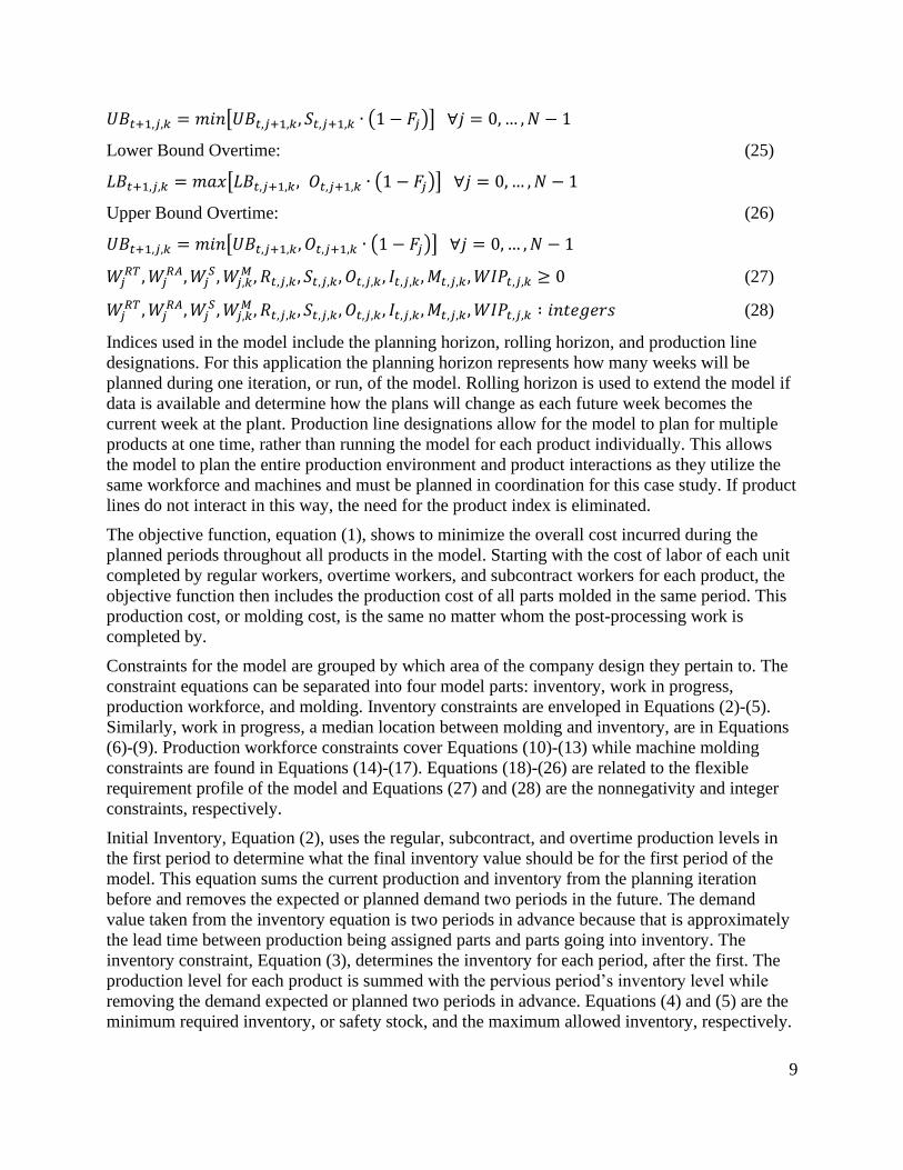
Indices used in the model include the planning horizon, rolling horizon, and production line

designations. For this application the planning horizon represents how many weeks will be

planned during one iteration, or run, of the model. Rolling horizon is used to extend the model if

data is available and determine how the plans will change as each future week becomes the

current week at the plant. Production line designations allow for the model to plan for multiple

products at one time, rather than running the model for each product individually. This allows

the model to plan the entire production environment and product interactions as they utilize the

same workforce and machines and must be planned in coordination for this case study. If product

lines do not interact in this way, the need for the product index is eliminated.

The objective function, equation (1), shows to minimize the overall cost incurred during the

planned periods throughout all products in the model. Starting with the cost of labor of each unit

completed by regular workers, overtime workers, and subcontract workers for each product, the

objective function then includes the production cost of all parts molded in the same period. This

production cost, or molding cost, is the same no matter whom the post-processing work is

completed by.

Constraints for the model are grouped by which area of the company design they pertain to. The

constraint equations can be separated into four model parts: inventory, work in progress,

production workforce, and molding. Inventory constraints are enveloped in Equations (2)-(5).

Similarly, work in progress, a median location between molding and inventory, are in Equations

(6)-(9). Production workforce constraints cover Equations (10)-(13) while machine molding

constraints are found in Equations (14)-(17). Equations (18)-(26) are related to the flexible

requirement profile of the model and Equations (27) and (28) are the nonnegativity and integer

constraints, respectively.

Initial Inventory, Equation (2), uses the regular, subcontract, and overtime production levels in

the first period to determine what the final inventory value should be for the first period of the

model. This equation sums the current production and inventory from the planning iteration

before and removes the expected or planned demand two periods in the future. The demand

value taken from the inventory equation is two periods in advance because that is approximately

the lead time between production being assigned parts and parts going into inventory. The

inventory constraint, Equation (3), determines the inventory for each period, after the first. The

production level for each product is summed with the pervious period’s inventory level while

removing the demand expected or planned two periods in advance. Equations (4) and (5) are the

minimum required inventory, or safety stock, and the maximum allowed inventory, respectively.

10

The safety stock commitment supports the company's customers if some part of the production

line is shut down, or the customer must place an emergency order. Generally, the safety stock for

this company is set to two times the six-month average demand for each product. Some products

have a manually set safety stock to help the company disregard any outliers in orders that have

arrived. The maximum inventory constraint prevents the inventory level from going too far over

the safety stock. This is generally set at two times the safety stock amount.

The work-in-progress (WIP) constraints, Equations (6)-(9), assist the production team with

determining when it is necessary to mold new parts or focus efforts on post-processing. Due to

the nature of the company, it is normal to keep a large safety stock of finished parts in inventory

as well as keep a large amount of molded parts ready for post-processing. Since the most

expensive part of production per unit is post-processing, the company does not see it as a major

loss if a product becomes discontinued while there are parts in WIP. Calculating the machined

parts of each period is completed using the maximum number of parts produced per mold and the

number of molds running. This value is added into the current WIP, through Equations (6) and

(7), as parts that have been molded are immediately considered WIP. Equation (6), initial work

in progress, computes the initial number of parts in WIP by using the machined parts of initial

period, subtracting the parts that have been assigned to post-processing with regular, overtime, or

subcontracted labor, and adding any WIP from the previous iteration. For each period after, the

WIP is calculated using Equation (7), setting WIP equal to the machined parts, minus the post-

processed parts of the same period, and adding the WIP from the previous period. Equations (8)

and (9) constrain the number of parts in WIP to a reasonable number. The minimum and the

maximum number of parts allowed in WIP is determined on a per-product basis. Products with

smaller demand, or new products, will be set with a maximum WIP around 1000, and a

minimum of 0. Established and high demand products' constraints for WIP is calculated based on

the previous 3-12 months of demand. Some of these products will allow a WIP capacity of 12

times the previous 3-month average demand, while others will be limited to 3 times the previous

12-month average demand. These constraints are adjusted when demand shows the need to do

so.

Within the company, there are some weeks where the regular, internal, workforce must post-

process parts as there is not another assignment for them. Therefore, there must be parts

available for this activity. Equation (10) dictates the minimum amount of parts needed for the

regular workforce each period based on the scheduled number of people that will be assigned to

post-processing and the maximum number of parts one person can complete in one period.

Across all product lines, the regular production level must be less than or equal to the total

available regular workers, including those not currently scheduled to work post-processing, times

the maximum number of parts one regular person can complete in one period. This is covered in

the capacity of the regular production constraint, Equation (11). Similarly, the capacity of the

subcontract production is set in Equation (12) and the capacity of the overtime production is set

in Equation (13). Overtime for post-processing activities is only assigned to subcontract workers

and therefore their workers are the only ones included in this calculation.

The maximum number of molds, Equation (14), shows that when the molds being used across all

products are added up, they should be less than the maximum number of molds allowed to run

for the given period, which is decided by the total number of machines available. The molds

11

available constraint, Equation (15), accounts for the company having a limited number of molds

for each product. It constrains the molds being used for each product to be less than or equal to

the number of molds available for that product in each period. The number of molds available for

each product can change on an as-needed basis, but there is a lead time for this transition

depending on the product. Mold production capacity, Equation (16), limits the parts needed for

posting to not exceed the molding capabilities. This prevents the production teams, internal and

external, from outpacing the molding capabilities and prevents the WIP from being taken down

to zero. Equations (17) sets the number of molds being run for each product equal to the total

production level given lead time divided by the capacity level of the molds for each product.

This constraint also sets the number of molds calculated to be an even number since molds at this

company are run in pairs. Equation (17), while nonlinear due to rounding operations, is

acceptable and can be linearized with the transformation has highlighted in Remark I.

The flexible requirement profile, Equations (18)-(20), sets the total production, of regular,

subcontract, and overtime, for each period, and each product line, to a lower and upper bound.

These bounds are calculated in Equations (21)-(25) for each iteration, period, and product line.

The lower bound, Equations (21), (23), and (25), is set for the next iteration using the maximum

between either the lower bound from the next period or the production level with lead time from

the next period times 1 minus the flexible limit of the current period. The upper bound,

Equations (22). (24), and (26), is set for the next iteration using the minimum between either the

upper bound of the next period or the production level with lead time times 1 minus the flexible

limit of the current period.

Equation (27) sets the following parameters as nonnegative; true regular workers, available

regular workers, subcontract workers, molds available, regular production, subcontract

production, overtime production, inventory, the number of molds being used, and the number of

parts in WIP.

Equation (28) sets the following parameters as integer values; true regular workers, available

regular workers, subcontract workers, molds available, regular production, subcontract

production, overtime production, inventory, the number of molds being used, and the number of

parts in WIP.

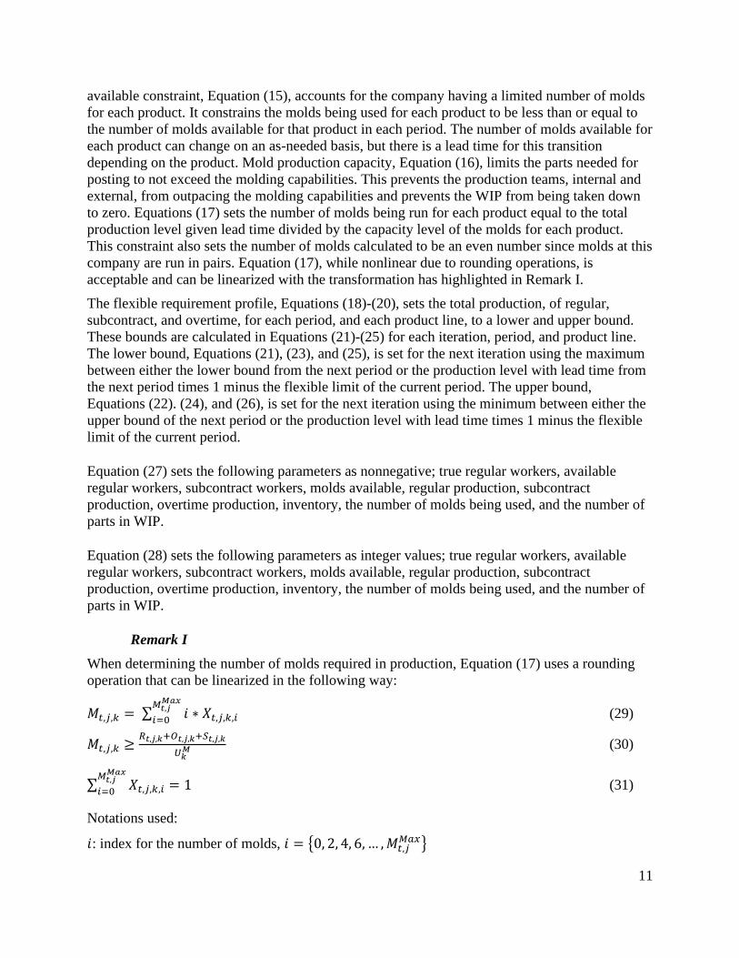
Remark I

When determining the number of molds required in production, Equation (17) uses a rounding

operation that can be linearized in the following way:

𝑀𝑡,𝑗,𝑘 = ∑ 𝑖 ∗ 𝑋𝑡,𝑗,𝑘,𝑖

𝑀𝑡,𝑗𝑀𝑎𝑥

𝑖=0 (29)

𝑀𝑡,𝑗,𝑘 ≥𝑅𝑡,𝑗,𝑘+𝑂𝑡,𝑗,𝑘+𝑆𝑡,𝑗,𝑘

𝑈𝑘𝑀 (30)

∑ 𝑋𝑡,𝑗,𝑘,𝑖

𝑀𝑡,𝑗𝑀𝑎𝑥

𝑖=0= 1 (31)

Notations used:

𝑖: index for the number of molds, 𝑖 = {0, 2, 4, 6, … , 𝑀𝑡,𝑗𝑀𝑎𝑥}

12

𝑋𝑡,𝑗,𝑘,𝑖: variable that is a j-step ahead binary indication of planned number of i molds in each

iteration t for each product line k

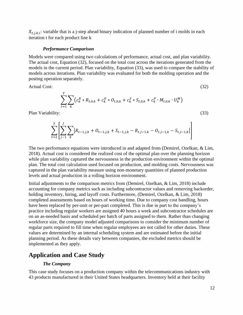
Performance Comparison

Models were compared using two calculations of performance, actual cost, and plan variability.

The actual cost, Equation (32), focused on the total cost across the iterations generated from the

models in the current period. Plan variability, Equation (33), was used to compare the stability of

models across iterations. Plan variability was evaluated for both the molding operation and the

posting operation separately.

Actual Cost: (32)

∑ ∑(𝑐𝑘𝑅 ∗ 𝑅𝑡,0,𝑘 + 𝑐𝑘

𝑂 ∗ 𝑂𝑡,0,𝑘 + 𝑐𝑘𝑆 ∗ 𝑆𝑡,0,𝑘 + 𝑐𝑘

𝑃 ∙ 𝑀𝑡,0,𝑘 ∙ 𝑈𝑘𝑀)

𝑘

𝑇

𝑡=1

Plan Variability: (33)

∑ [∑ ∑|𝑅𝑡−1,𝑗,𝑘 + 𝑂𝑡−1,𝑗,𝑘 + 𝑆𝑡−1,𝑗,𝑘 − 𝑅𝑡,𝑗−1,𝑘 − 𝑂𝑡,𝑗−1,𝑘 − 𝑆𝑡,𝑗−1,𝑘|

𝑘

𝐽

𝑗−1

]

𝑇

𝑡=2

The two performance equations were introduced in and adapted from (Demirel, Ozelkan, & Lim,

2018). Actual cost is considered the realized cost of the optimal plan over the planning horizon

while plan variability captured the nervousness in the production environment within the optimal

plan. The total cost calculation used focused on production, and molding costs. Nervousness was

captured in the plan variability measure using non-monetary quantities of planned production

levels and actual production in a rolling horizon environment.

Initial adjustments to the comparison metrics from (Demirel, Ozelkan, & Lim, 2018) include

accounting for company metrics such as including subcontractor values and removing backorder,

holding inventory, hiring, and layoff costs. Furthermore, (Demirel, Ozelkan, & Lim, 2018)

completed assessments based on hours of working time. Due to company cost handling, hours

have been replaced by per-unit or per-part completed. This is due in part to the company’s

practice including regular workers are assigned 40 hours a week and subcontractor schedules are

on an as-needed basis and scheduled per batch of parts assigned to them. Rather than changing

workforce size, the company model adjusted comparisons to consider the minimum number of

regular parts required to fill time when regular employees are not called for other duties. These

values are determined by an internal scheduling system and are estimated before the initial

planning period. As these details vary between companies, the excluded metrics should be

implemented as they apply.

Application and Case Study

The Company

This case study focuses on a production company within the telecommunications industry with

43 products manufactured in their United States headquarters. Inventory held at their facility

13

includes 883 different products, and, including kits, there are 1,481 part numbers to track and

plan for. For the fiscal year of 2019, the company completed over 87,000 orders including more

than 128 M shipped parts. Approximately 59% of these parts were shipped the same day or the

next day, and 80% of the orders were shipped within seven calendar days.

For the 43 in-house manufactured parts, there are five main production types within the plant

ranging from ten machine capacity to one machine capacity with cycle times varying on the

product level and personnel requirements. The study focused on the top six highest demand, in-

house manufactured parts, within the same production type. These products are commonly sent

to a subcontractor for post-processing to be completed. While a base number of parts are post-

processed within the facility, the in-house staff is focused on the manufacturing and quality

control of parts and specialty-part post-processing. The subcontractor completes the post-

processing steps of high-demand parts from two of the five production types.

Given the demand style of the telecommunications industry, the company keeps a standard safety

stock of two times their six-month average for every part manufactured at their main facility,

adjusting for outliers where necessary. Parts brought in from other manufacturing plants also

have a high safety stock that is individually determined based on their lead times and typical

demand. Along with a large safety stock of finished parts in inventory, the company stores parts

that are considered unfinished, work-in-progress (WIP), parts. The amount of WIP parts required

is determined on a per-product basis. Some products require 3 years expected demand in WIP

while others have a WIP capacity and no minimum level of WIP. When determining when to

manufacture new parts or post-process parts, inventory and WIP values are considered along

with the demand. A closer look at how WIP and inventory interact within the production

dynamic is shown in Figure 1 covering the company's production plan.

Separating interactions that affect production can be done with three groups including the

customer service team, the production team, and the shipping team. Each group is responsible for

ensuring parts are promised and delivered to customers on a timely and consistent basis.

Majority of the orders, or parts sold, originate in the customer service department from historic

orders that include long-term planned commitments, new projects that are developed rapidly in

industry, or undisclosed work which are from companies that are not major industry players and

only need a few parts for experimental purposes. While preparing purchase orders for these

customers, there is also forecasted orders being theoretically committed based on industry insight

and planned upcoming projects. The customer service team will consider these avenues for

product commitments and check within our inventory to make sure we can meet the requested

ship-by date.

If the inventory is high and expected to remain relatively high after an order is completed, the

customer service team will schedule the shipment with our shipping team who then ensures parts

are delivered to the customer. If the inventory is low or will otherwise become low after an order

is completed, the customer service team will alert production of the order requested to determine

the next best steps.

Once production is alerted to a low or soon-to-be low inventory, the production team will check

their WIP vs inventory levels as well as the current week’s planned production to determine the

next steps. With a high WIP and stable inventory, customer service will be instructed to schedule

the shipment. When there is a low WIP and low inventory, the customer service team will be

14

provided a future-commitment date while the team then schedules both molding and post-

processing. Similarly, a high WIP and low inventory will trigger a future-commitment date for

the customer service team and scheduling of post-processing parts.

Post-processing within production is divided between two groups, the internal process, and the

subcontracted process. As mentioned, the internal workforce can provide a baseline of parts due

to the company structure. Although, unless they are specialty parts, the internal workforce

focuses on quality assurance, measurement, and manufacturing positions rather than post-

production. Taking on the majority of the post-processing is the subcontracted team. They are

both the cheaper option and can finish parts at a faster pace than the internal workforce.

However, their lead time on assigned parts can exceed that of the internal group due to shipping.

Once parts have been sent from molding, into WIP, and post-processed, they are entered into

inventory as finished parts ready for shipping by the shipping team.

Application

The case study applied aggregate production planning with flexible requirement profiles to a

manufacturing facility in the telecommunications industry assisting in the determination of the

optimal production schedule. Variables within the model being scheduled for each product

included the number of molds running, the number of parts that should be assigned into post-

production for the internal, subcontract, and overtime workforce, the number of parts in

inventory, and the number of parts in WIP.

Like any business, there is nervousness within the demand values placed within the model.

Current planning practices at the company include meeting once a week to discuss the planned

shipments for the week, upcoming commitments, forecasts, current inventory and WIP levels,

and production plans. General nervousness is covered in these discussions, but with unexpected

orders becoming more frequent, and the volatility of the telecommunications industry, a planning

model will prevent emotions from tying into production decisions that currently cause

unpredictability within the plant. Nervousness was captured within the model using flexible

requirement profiles for the production levels on the rolling horizon. To stabilize production and

molding, as the week planned gets closer to being the current week, the flexibility of the

production plan decreases.

Four versions of the model formulation were applied to the case study data sample. The first

distinction being how the plans change if WIP is included in the planning process. Second, the

APP-FRP model was compared to an APP model alone. The four models included in the

comparison are distinguished as follows: Aggregate production plan without WIP (APP-

NONWIP); Aggregate production plan with WIP (APP-WIP); Aggregate production plan with

flexible requirement profile without WIP (APP FRP-NONWIP); Aggregate production plan with

flexible requirement profile with WIP (APP FRP-WIP).

Between the FRP models, different flex limit ranges, located in Table 1, were evaluated to

determine its effect on the overall plan and if there was an ideal spot for the company to use.

Within the ideal flex limit set up, a sensitivity analysis was completed on the regular

true/scheduled workforce (WRT) values. These evaluations were used to determine how the two

parameters changed the plan results within the plan variability and actual cost. These tests were

also compared to the true plan that the company implemented during the time of data collection

to determine if there was any benefit or correlation to the proposed APP-FRP plans.

15

Challenges

Challenges within this case study presented themselves around capturing the nuances of the

company operation and when deciding on a data set to use. While these challenges were

overcome, they will be covered to assist in future applications and to describe how the company

is unique in its own application.

Data challenges began when only 2020 and limited 2019 data was available for all parameters.

The company largely only keeps WIP and inventory data for 7 months at a time whereas demand

data is kept permanently within the sales and shipping tracking system. Weekly mold

assignments are not generally stored and therefore was only tracked once the study was started.

Near the end of the 2019 year, when data was available, the company had a low demand due to

industry slow-down once the 2018 projects, which were abnormally high, were finalized and

wrapped up. Keeping the business running and preparing for an expected higher demand in 2020,

the company’s metrics were not normal and therefore could not be used for the study. A few

products exceeded their maximum inventory levels during this time to assist the subcontracting

company to stay open and internal employees were used to assist in developing new products

rather than continuing normal production. During 2020, once Covid-19 began to cause closures

within the United States, the company had an alternative work schedule, splitting the production

team in half and placing them on a weekly rotation, for part of the year. This decreased the total

level of production and caused them to heavily rely on the WIP, safety stock, and subcontractors

to meet demand. Additionally, as uncertainty rose surrounding businesses and boarders

remaining open, many international customers doubled or tripled their product demands to create

their own form of safety stock. As 2020 continued with things going back to some form of

normal as far as production is considered, the company kept the high demand, even as the

customer fears were lessened, due to industry projects being pushed forward from pending

election results and company mergers. Though some products used their safety stock during

these times, the company was still able to meet all of the demand on time for all customers, as

this is what safety stock is for. While 2020 presented some abnormal data regarding inventory

and WIP levels, there were some months that could be extracted for the study and applied as

normal or slightly modified to fit the expected normal. The model does not allow the use of the

safety stock but does ensure that it is maintained when possible. Months were the safety stock

will need to be used due to abnormal events, like months of 2020 have shown, can be adjusted

within the model to decrease the minimum inventory level on a product-by-product and week-

by-week basis.

After determining the most applicable set of data, the inclusion of multiple products within one

production operation was implemented on the base model. This necessitated the new index, k,

and work to identify which parameters and variables required it. This index increased the

complexity of the model by adding a third dimension for some parameters. Previous experiences

with APP-FRP that this case study is based on, (Demirel E. , 2014), (Demirel, Ozelkan, & Lim,

2018) and (Torabzadeh & Ozelkan, 2016), did not include this third dimension. The parameters

that required the product index include labor costs, units produced per mold, estimated demand,

safety stock and WIP minimum and maximum, the number of molds available, the lower and

upper bounds. All variables were determined on a per product basis.

The parameters not given a product index are those that either vary so little between products

that the change is negated, or they are consistent no matter the product. These parameters include

16

the maximum number of units that can be posted by an individual, the scheduled workforce

internally and at the subcontractor, the maximum number of molds that can be ran, and the flex

limits. Posting within this production line does not vary product-to-product enough to be

considered in the evaluation as all products of this type are posted the same way. The maximum

is also averaged and varies per person which is not included in this model. As mentioned, the

workforce is not determined by the model, but it is included to assist with determining the post-

molding production limitations. Since individuals are not assigned specific products and all

products of this line are posted the same way, the workforce does not need to be defined per

product line. However, the model does determine which products the workforce will post each

period. Like posting, the model determines which parts will be molded each period. Rather, the

model determines which molds will be ran. To set a maximum for this across the combination of

products, the maximum number of molds is based on how many machines are available. Since

the model only included one production type, and all machines in this type can run all products,

the maximum number of molds that can be ran did not require the product index. Finally, the flex

limits are based on the post-production type, regular, subcontract, or overtime. This covers the

change allowed across the entire production process and was not decided on a per product basis

as the same workforce and machines will be used across all products included.

Deciding on the type of flex limit arrangement that would suit the company and therefore

adjusting how much change could occur between planning iterations depends on company

culture, production interactions, and ability to afford the plan that could reduce nervousness in

the production team. Due to the method of planning within the company, where meetings are

held at the beginning of the period and the plan is implemented for the current period and mostly

set for the next, the flex limit of period zero was initially set at zero percent. This allows for a

level of consistency within the scheduling and aligns with the company culture. Furthermore,

this allows the company its next or same day shipping on majority of their products. Since they

know what is being produced that week and with some certainty next week, they know what will

be replenished if it is near its safety stock or otherwise has low inventory and can make shipping

commitments accordingly. While this case study allowed for a zero percent flex limit at period

zero to be reasonable and attainable, the model is set up in a way that it can be changed for

different applications where that is not realistic or desired. This ability to change the flex limits

easily has also allowed a sensitivity analysis to be completed on how flex limits change the

outcome within the company’s cost and plan variability to determine the ideal arrangement and

allowable limits to stay comfortable within their production environment.

Nonlinearities posed a challenge for this APP study, as it is solved using the linear programming

method. For this company, nonlinearity appeared during the molding considerations through the

requirement that product molds be ran in pairs. Through the use convergent rounding, this

constraint was achieved within the model formulation. Through Remark I, the nonlinearity was

removed from the model by separating the single constraint into three constraints that achieved

the same influence on the model. Remark I also introduced parameter “X”, which was a binary

indication of the planned number molds to run for each product, and index “i”, containing the

options available for the number of molds to become. “i” was a list of even values ranging from

0-20 as 20 was the maximum number of machine molds available for production to run.

17

Results

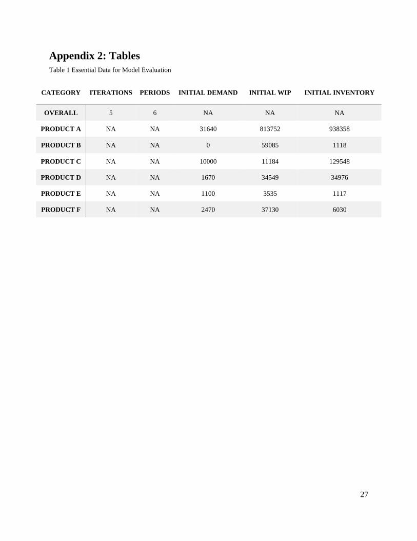
To establish model performance within the company application, the data applied remained the

same amongst the APP-NONWIP, APP-WIP, APP FRP-NONWIP, and APP FRP-WIP models.

Essential data to start the models, such as periods, iterations, products, initial demand, initial

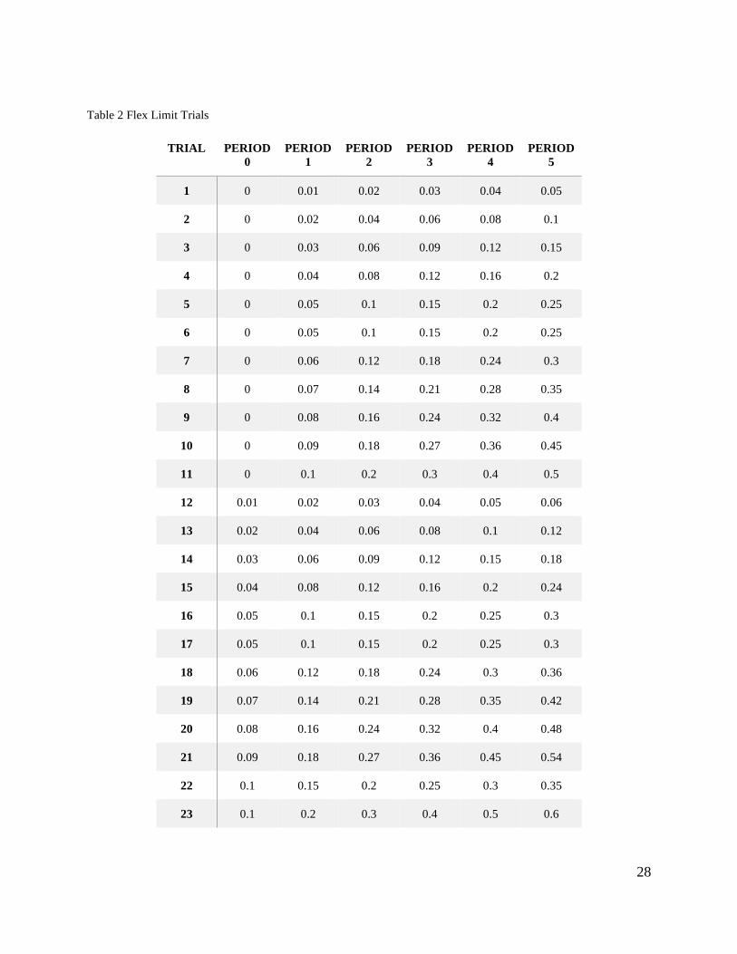
WIP, and initial inventory, can be found in Table 1. While the remainder of the parameters used

were obtained from the company, they are not being reported.

Two analyses were completed using the four models. One being a comparison between flex

limits within the FRP models and the other comparing model performances while changing

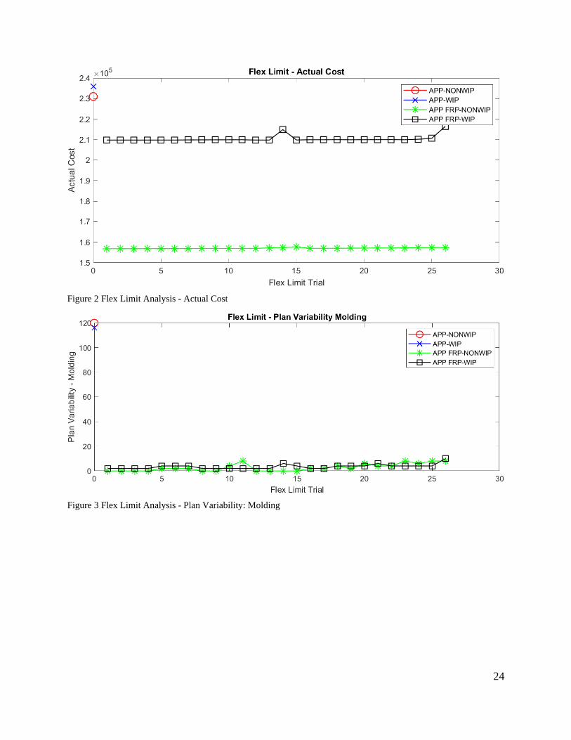
WRT values. The FRP models were placed through 26 flex limit trials as described in Table 2

with a WRT value of 3. All four models were placed through 11 consecutive values, 0- 10, for

WRT while the flex limits, where applicable, remained at the ideal values found through the flex

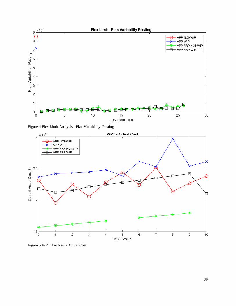
limit trials, trial 1. Figures 2-4 show the results for actual cost, plan variability – posting, and

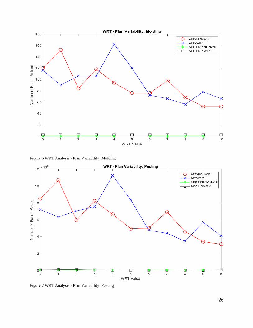
plan variability – molding for the flex limit comparisons. Figures 5-7 present results for the WRT

comparison. The following section will discuss what was found during the two sensitivity tests

completed and a basis for choosing an optimal environment for the company to use moving

forward.

The APP models, both the NONWIP and WIP version, reported substantially higher cost and

plan variability across most tests and trials completed compared to those paired with FRP. The

APP models are set as trial 0 in Figures 2-4. Comparing the actual cost of the plans there is only

one instance found in this study that shows having required WIP values is more advantageous

than doing without. This is found when WRT is set to 5, requiring the model to include parts for

five internal production staff to be available for posting. Within this instance, the WIP does not

show great advantage over the NONWIP version, and overall, it does not interest the company to

keep five full time staff in the internal posting position. An additional note for the comparison of

just APP models is that the difference between the WIP and NONWIP models when comparing

actual cost and production variability, the differences may be allowable when there are no

internal posting requirements. Their differences are considerable once there is an internal posting

requirement. While the WIP environment shows a higher cost, it also shows a generally lower

plan variability in both the molding and posting requirements providing a more stable

environment for the production and molding teams. So, when considering a pure APP model, the

NONWIP production environment is a more consistently cheaper option for the company,

although it does not align with their current operation that focuses on stability within the plant.

With the APP models performing as a starting point for the production planning operation, using

models with the FRP attribute can be seen to offer an advantage for the case study applied.

Within the flex limit trials, Figures 2-4, the APP-FRP models both had a lower actual cost and a

lower plan variability for posting and molding. These differences were nonminimal and show

that a great advantage is available to the company when they implement the flexible requirement

profile strategy to their production operation. Again, the WIP inclusive model shows a higher

actual cost than the NONWIP version, as expected, but also consistently presented a lower plan

variability among majority of the flex limit trials. Therefore, even with changes within the flex

limits of the model, the WIP version has better plant stability.

Within the flex limit trials, trial 1 limits presented the lowest cost and lowest posting plan

variability for both the WIP and NONWIP versions of the APP-FRP models with a WRT value

18

of 3. As mentioned, having a zero percent change on the first iteration works for this application

because the company puts a high priority on stability between weeks and reduced nervousness

within the plant. This aligns with their current operation techniques and provides evidence that

the model is suited for their application.

Using the trial 1 flex limitation values on the APP-FRP models, the four models were placed

through a WRT evaluation. Changing WRT between zero and ten allowed for 11 environments

to be analyzed and show how mandating internal posting operations effects the actual cost and

stability of the plant. Two outliers, WRT of 5 and 10, were found within the APP-FRP-NONWIP

model. These values caused the model to determine there was no optimal path with the current

set of parameters for the 5th iteration. To keep the analysis fair across models, these results were

excluded.

For actual cost during the WRT sensitivity analysis, the APP models are more sporadic in their

reported values as the WRT value increases showing little correlation between the number of

scheduled internal workforce and the actual cost of the plan. However, the APP-FRP models

showed a positive correlation between increasing scheduled internal workforce and the actual

cost of the model. The cheapest option should be when WRT is set to zero and all posting

operations are sent to the subcontractor until its limit is reached as it is a cheaper and more

efficient option than having the regular, internal, workforce complete this work. This relationship

is shown with the APP-FRP-NONWIP model and is close, but not exactly shown, with the APP-

FRP-WIP model due to a decrease when WRT is set to ten. Both APP-FRP models were more

cost effective than the APP-WIP model and the APP-NONWIP was found to randomly oscillate

around the actual cost the FRP-APP-WIP option. The APP-FRP-NONWIP model was the most

cost effective, and consistent, planning operation for the company regarding increasing WRT

values.

Plan variability in posting and molding, regarding WRT values, show identical patterns for each

APP model respectively. The plan variability values for the APP-FRP models comparatively to

the APP models can be considered zero. Adding the FRP to the model presented a substantially

less variable production plan for both WIP and NONWIP environments. Between the two APP-

FRP models, the WIP environment proved to be more stable in posting quantities than the

NONWIP in five of the nine applicable WRT values. For molding plan variability, the NONWIP

environment showed variability of 0 between weeks while the WIP environment has a plan

variability of 2. This result for the WIP model is considered an allowable level of flexibility

between weeks as the company has a process in place to cover that level of change and can

therefore be ignored when deciding which plan is optimal for their application.

Summary and Conclusion

The telecommunications industry is a changing environment with multiple levels of production,

regulations, and services provided. The company used for this case study is involved in

providing connector products that are used around the world with applications including

computer systems, data centers, and fiber to the home. When large projects are announced with

specific distributers, the company can safely assume their products will part of the solution being

implemented. However, not all projects come to fruition and some projects are underestimated

and demand spikes for years. While the industry is essential to the operation of day-to-day life

and future innovation and expansion of society, it is volatile and somewhat random between

19

years from project delays and derailment to projects advancing faster and larger than expected.

This volatility creates a delicate and specific level of infrastructure for the company in the case

study to be able to sustain this type of market.

Within the company being analyzed, there are 43 internally manufactured products that are

dispersed among five production types. Of these five production types, the one selected for this

study involves ten machines that operate interchangeably to support various product lines and

two types of workforces that get products ready for inventory and customers. Including the

connections between product lines required the model to have a multiproduct aspect that had not

been explored within the APP FRP application. The case study proved that this could be

incorporated successfully with all intricacies and connections including within the constraints of

the model.

Additionally, with the intermediate step of post-processing between molding and inventory, the

company also involves a work-in-progress type of product. The company includes this WIP in

their production planning as a secondary type of safety stock that keeps their products available

during the high demand market times when manufacturing cannot meet the required level of

molding. WIP is also used to gauge if orders can be met within an acceptable timeframe and to

determine when deliverable times can be expected to keep the customers expectations realistic.

The model determined that including this WIP did increase the stability of the production

environment of the company and assist them with this priority while keeping their high demand

levels met and all minimum requirements met for inventory and production.

The model that performed the closest to the company’s current operation and can assist in

removing the emotional response from their production environment and therefore decrease

variability more and reducing costs was the APP FRP-WIP model. This model includes the

multiproduct aggregate production planning with flexible requirement profiles and involves the

WIP levels that the company relies on at this time. The model performed as expected with higher

costs compared to a non-WIP environment, increasing costs as internal workforces required

parts, and keeping the plan variability low to reduce nervousness within the production team.

The multiproduct APP FRP methodology can be applied to this specific case study and provide

increased performance results of a manufacturing plant in the telecommunications industry and

can include two types of inventory levels and associated intricacies.

20

References

Baker, K. (1977, January). An Experimental Study of the Effectiveness of Rolling Schedules in

Production Planning. Decision Sciences, 8(1). doi:https://doi.org/10.1111/j.1540-

5915.1977.tb01065.x

Baker, K., & Peterson, D. (1979, April). An Analytic Framework for Evaluating Rolling

Schedules. Management Science, 25(4), 341-351.

Buzacott, & Shanthikumar. (1994). Safety STock Versus Safety Time in MRP Controlled

Production Systems. Management Science, 40(12), 1678-1689.

Calrson, Robert, Jucker, & Kropp. (1979). Less Nervous MRP Systems: A Dynamic Economic

Lot-Sizing Approach. Management Sciences, 25(8), 754-761.

Chung, C., & Krajewski, L. (2007, June). Replanning Frequencies for Master Production

Schedules. Decision Sciences, 17(2), 263-273. doi:10.1111/j.1540-5915.1986.tb00225.x

Chung, C.-H., Chen, I.-J., & Cheng, G. (1988, December). Planning Horizons for Multi-Item

Hierarchical Production Scheduling Problems: A Heuristic Search Procedure. European

Journal of Operational Research, 37(3), 368-377.

Costanza. (1996). Quantum Leap: In Speed to Market. Jc-I-T Institute of Technology.

Demirel, E. (2014). Flexible Planning Methods and Procedures With Flexibility Requirements

Profile. University of North Carolina at Charlotte. Charlotte, NC: University of North

Carolina at Charlotte.

Demirel, Ozelkan, & Lim. (2018). Aggregate Planning with Flexibility Requirements Profile.

International Journal of Production Economics, 45-58.

doi:https://doi.org/10.1016/j.ijpe.2018.05.001

Graves. (2011). Uncertainty and Production Planning. Planning Production and Inventories in the

Extended Enterprises. Springer US, 82-101.

Graves, S. (2008). Uncertainty and Production Planning. Cambridge, MA: MIT.

doi:10.1007/978-1-4419-6485-4_5

Hafezalkotob, A., Chaharbaghi, S., & Lakeh, T. M. (2019). Cooperative Aggregate Production

Planning: A Game Theory Approach. Journal of Indutrial Engineering International,

S19-S37. doi:https://doi.org/10.1007/s40092-019-0303-0

Holt, Modigliani, & Herbert. (1955). A Linear Decision Rule for Production and Employment

Scheduling. Management Science, 2(1), 1-30.

Holt, Modigliani, & Muth. (1956). Derivation of a Linear Decision Rule for Production and

Employment. Management Science, 2(2), 159-177.

Inman, & Gonsalvez. (1997). Measuring and Analyzing Supply Chain Schedule Stability: A

Case Study in the Automotive Industry. Production Planning & Control, 64(1), 194-204.

Jamalnia, A., Yang, J.-B., Feili, A., Jamali, D.-L. X., & Gholamreza. (2019). Aggregate

Production Planning Under Uncertainty: A Comprehensive Literature Survey and Future

21

Research Directions. The International Journal of Advanced Manufacturing Technology,

159-181. doi:https://doi.org/10.1007/s00170-018-3151-y

Kadipasaoglu, & Sridharan. (1995). Alternative Approaches for Reducign Schedule Instability in

Multistage Manufacturing Under Demand Uncertainty. Journal of Operations

Management, 13(3), 193-211.

Kamien, & Li. (1990). Subcontracting, Coordination, Flexibility, and Production Smoothing in

Aggregate Production Planning. Management Science, 36(11), 1352-1363.

Koh, Gunasekaran, & Saad. (2005, August 1). A Business Model For Uncertainty Management.

Benchmarking: An International Journal, 12(4).

doi:https://doi.org/10.1108/14635770510609042

Kok, T. d., & Inderfurth, K. (1997, November). Nervousness in Inventory Management:

Comparison of Basic Control Rules. European Journal of Operational Research, 103(1),

55-82. doi:https://doi.org/10.1016/S0377-2217(96)00255-X

Lee, H., Padmanabhan, V., & Whang, S. (1997, April). Information Distortion in a Supply

Chain: The Bullwhip Effect. Management Science, 43(4), 546-558.

doi:https://doi.org/10.1287/mnsc.1040.0266

Lin, N.-P., Krajewski, L., Leong, K., & Benton, W. (1994, March). The Effects of

Environmental Factors on the Design of Master Production Scheduling Systems. Journal

of Operations Management, 11(4), 367-384. doi:https://doi.org/10.1016/S0272-

6963(97)90005-X

McClain, J., & Thomas, J. (1977, March). Horizon Effects in Aggregate Production Planning

with Seasonal Demand. Management Science, 23(7), 667-787.

doi:https://doi.org/10.1287/mnsc.23.7.728

Meixell. (2005). The Impact of Setup Costs, Commonality, and Capacity on Schedule Stability:

An Exploratory Study. International Journal of Production Economics, 95(1), 95-107.

Sridharam, & Berry. (1990). Master Production Scheduling Make-to-Stock Products: A

Framework For Analysis. The International Journal of Production Research, 28(3), 541-

558.

Sridharan, & LaForge. (1989). The Impact of Safety Stock on Schedule Instability, Cost and

Service. Journal of Operations Management, 8(4), 327-347.

Sridharan, Berry, & Udayabhanu. (1987). Freezing the Master Production Schedule Under

Rolling Planning Horizons. Management Science, 1137-1149.

Srinivasan, M. (2004). Streamlined: 14 Principles for Building & Managing the Lean Supply

Chain (1 ed.). Mason, Ohio: Thomson Business & Professional Publishing.

Torabzadeh, S., & Ozelkan, E. (2016). A Fuzzy Programming Approach For Aggregate

Production Planning With Flexible Requirement Profiles. American Society for

Engineering Management 2016 International Annual Coference. American Society for

Engineering Management.

Wagner, H., & Whitin, T. (1958, October). Dynamic Version of the Economic Lot Size Model.

Management Science, 5(1), 89-96.

22

Yano, & Carlson. (1987). Interaction Between Frequency of Rescheduling and the Role of Safety

Stock in Material Requirements Planning Systems. International Journal of Production

Research, 25(2), 221-232.

Zhao, & Lee. (1993). Freezing the Master Production Schedule For Material Requirements

Planning Systems Under Demand Uncertainty. Journal of Operations Management,

11(2), 185-205.

23

Appendix I: Figures

Figure 1 Company Structure for Customer Service, Production and Shipping

24

Figure 2 Flex Limit Analysis - Actual Cost

Figure 3 Flex Limit Analysis - Plan Variability: Molding

25

Figure 4 Flex Limit Analysis - Plan Variability: Posting

Figure 5 WRT Analysis - Actual Cost

26

Figure 6 WRT Analysis - Plan Variability: Molding

Figure 7 WRT Analysis - Plan Variability: Posting

27

Appendix 2: Tables

Table 1 Essential Data for Model Evaluation

CATEGORY ITERATIONS PERIODS INITIAL DEMAND INITIAL WIP INITIAL INVENTORY

OVERALL 5 6 NA NA NA

PRODUCT A NA NA 31640 813752 938358

PRODUCT B NA NA 0 59085 1118

PRODUCT C NA NA 10000 11184 129548

PRODUCT D NA NA 1670 34549 34976

PRODUCT E NA NA 1100 3535 1117

PRODUCT F NA NA 2470 37130 6030

28

Table 2 Flex Limit Trials

TRIAL PERIOD

0

PERIOD

1

PERIOD

2

PERIOD

3

PERIOD

4

PERIOD

5

1 0 0.01 0.02 0.03 0.04 0.05

2 0 0.02 0.04 0.06 0.08 0.1

3 0 0.03 0.06 0.09 0.12 0.15

4 0 0.04 0.08 0.12 0.16 0.2

5 0 0.05 0.1 0.15 0.2 0.25

6 0 0.05 0.1 0.15 0.2 0.25

7 0 0.06 0.12 0.18 0.24 0.3

8 0 0.07 0.14 0.21 0.28 0.35

9 0 0.08 0.16 0.24 0.32 0.4

10 0 0.09 0.18 0.27 0.36 0.45

11 0 0.1 0.2 0.3 0.4 0.5

12 0.01 0.02 0.03 0.04 0.05 0.06

13 0.02 0.04 0.06 0.08 0.1 0.12

14 0.03 0.06 0.09 0.12 0.15 0.18

15 0.04 0.08 0.12 0.16 0.2 0.24

16 0.05 0.1 0.15 0.2 0.25 0.3

17 0.05 0.1 0.15 0.2 0.25 0.3

18 0.06 0.12 0.18 0.24 0.3 0.36

19 0.07 0.14 0.21 0.28 0.35 0.42

20 0.08 0.16 0.24 0.32 0.4 0.48

21 0.09 0.18 0.27 0.36 0.45 0.54

22 0.1 0.15 0.2 0.25 0.3 0.35

23 0.1 0.2 0.3 0.4 0.5 0.6

29

24 0.15 0.2 0.25 0.3 0.35 0.4

25 0.2 0.25 0.3 0.35 0.4 0.45

26 0.25 0.3 0.35 0.4 0.45 0.5