Multirate Signal Processing, DSV2Introduction

Lecture: Mi., 9-10:30 HU 010

Seminar: Do. 9-10:30, K2032 (bi-weekly)

Our Website contains the slides

www.tu-ilmenau.de/mt → Lehrveranstaltungen → Master → Multirate Signal Processing

We also have a Moodle 2 website, at

https://moodle2.tu-ilmenau.de/course/view.php?id=395

which will contain the newest slides and the weekly quiz assignments (to be done individually).

There will be bi-weekly homework assignments, which will count 30% towards the final grade. The quizzes are part of the homework, and will count as 25% of the

homework. To pass the course you need to pass the final exam.

We have Python Homework, which can be done in groups of max. 3 people.

The course has 5 LP (Credit Points), each LP is about 2-3 hours per week, which means we have 10-15 hours total per week or about20 hours for 2 weeks (the homework cycle).

We will use the system Moodle2 for information exchange and for our quiz assignments, at:

https://moodle2.tu-ilmenau.de/login/index.php

where you need to sign up.

Prerequisite: the course Advanced Digital Signal Processing or DSP2, or thecorresponding knowledge.

Python is a very high level programming language, which contains the convenience and capabilities of Matlab/Octave, but is a full fledged programming language with

many more capabilities and libraries. It is Open Source and hence free to download and use. It can be installed under Windows, but under Linux it is already installed, and additional libraries are more easily installed under Linux. In general programming is much easier under Linux, because that is an operating system made for scientists, engineers, and programmers, unlike Windows, which is made for office applications.

Hence we will use Linux, and only support Linux (you can use Windows but then you are on your own).

Linux is also Open Source, and can be freely downloaded and used (unlike Windows, which is closed source and costs about 100 eur per copy!) Linux can be easily installed as a dual boot system or on “VirtualBox” as a virtual system on your Laptop or PC, for instance by downloading the system from www.ubuntu.com – Download -Overview. Download either “Desktop” for laptops or desktop computers, or Ubuntu-Flavours – Ubuntu Mate for Netbooks or the

Raspberry Pi. Then burn it to a USB stick or SD card, and then start the installation for instance by restarting the PC, keep F2 or F12or so constantly pressed to get into the Boot menu, and then choose “start from USB” or such. From there you can install Ubuntu as a dual boot.

Alternatively, you can also install Linux under “Virtual Box” on your PC or Laptop or Netbook, which is a virtual machine (a program which acts like a different computer).

Here is a short installation guide:

-Install in Windows:

Install VirtualBox and VirtualBox-Extensions from virtualbox.org

Download .iso image from www.ubuntu.com or https://ubuntu-mate.org/download/ (for

lightweight laptops) to usb stick or the PC hard drive

-Start VirtualBox, Setup "New Machine" using the iso image. After finishing, remove the iso image (if it is on the hard drive, rename it to avoid the installation to start again)

-Before starting the virtual machine in VirtualBox:

Set RAM and Number of CPU's high, in Settings-System-Processor

(http://askubuntu.com/questions/365615/how-do-i-enable-multiple-cores-in-my-virtual-enviroment)

-After starting the virtual machine, install guest additions. Open a terminal Window, e.g. with keyboard shortcut Strg-Alt-T. Then type:

sudo apt install virtualbox-guest-additions-iso

cd /media/schuller/VBOXADDITIONS...

sudo sh ./VBoxLinuxAdditions.run

(See: wiki.ubuntuusers.de/VirtualBox/Installation)

-Then restart the virtual machine.

Press (right)Strg-F for full screen mode

-Activate external Devices for the virtual machine:

USB: On top menu bar of the VirtualBox go to Devices-USB click for checkmark

Webcam: on the VirtualBox menu bar go to Devices-Webcam, click for checkmark.

Scientific Literature WorkWhen reading papers, check each information you deem as important by reading the corresponding references and check them by checking their references, until you reach the source of the information.

For information that is claimed as original, do an internet search on similar results.

For formulas, check them by programming them (e.g. in Python), and see if you can reproduce the results presented in the paper. If there is not enough information to reproduce the results,or the results differ significantly, that is a bad sign.

For paper writing, reference every information that you deem important or relevant to the source where you‘ve got yourinformation from. These references are important for reproducible research, and they are also the „currency“ of science, because scientists get their reputation from

other people referencing them. Omitting them is like „stealing“ or cheating.

If you are presenting algorithms or programs, present them in formulas or pseudo-code in such a way that other peoplecan reproduce your results (again, reproducable research). Check your formulas by programming them yourself, and see if they work. If you get error messages or wrong results, this shows that your formula has a problem.

-Goal of the course: To be able to solve problems in the area of Multirate Signal Processing, like how to design sampling rate converters or filter banks.

-Approach: Memorize only the most basic facts or properties, like the definition of the z-transform, then know how to use them (like how to derive the z-transform of a delayed signal). This is a skill.

As an Engineer, we need to get something towork or to function in the end. Engineering is also like applied physics, we need the theory and then the experimental verification.

It is recommended to read the slides before a lecture, such that we can answer questions during the lecture, and include the answers in the slides. Hence the slides will be kept in editing mode.

I will read each paragraph, and then ask for questions.

Course Book: Gilbert Strang, Truong Nguyen: “Wavelets and Filter Banks”

Ein deutsches Buch:

N. Fliege, "Multiraten-Signalverarbeitung: Theorie und Anwendungen", Teubner, Stuttgart, 1993

Lectures (as opposed to pure electronic learning) have the advantage that we can talk to each other, and that in this way the content can be tailored to your background. So you should ask questions, and also short discussions are beneficial in this way.

What is Multirate Signal Processing?

Multirate: meaning different sampling rates, as from using downsampling or upsampling. In filter banks, we reduce the sampling rate after filtering a signal, which reduces the bandwidth. For reconstruction and obtaining the original sampling rate, we need to up-sample and filter (for interpolation) the signal.

Where is Multirate Signal Processing used?

For instance in coding and compression algorithms, like the

so-called Modified Discrete Cosine Transform (MDCT) filter bank in audio coding, or the

Discrete Cosine Transform (DCT) in image or video coding

Channel coding (OFDM), where a channelis divided into many narrower channels with lower data rates and hence longer

symbol duration, to reduce problems with multipath/reflections

Example of a discrete time signal:

Typical sampling rate of audio from a CD:

44100 samples/second, or

44.1 Khz sampling rate.

Python example for a live plot of a microphone signal:

python pyrecplotanimation.py

The Nyquist theorem tells us: Our signal needs to be band limited to

less than half the sampling frequency, here: less than 22.05 kHz. Half the sampling frequency is also called the Nyquist frequency.

For time discrete signals we only use normalized frequencies, normalized tothe sampling frequency or the Nyquist frequency. For the latter, the normalized frequency of 1 would be the Nyquist frequency. Often you also findπ as the Nyquist Frequency.

Simple sample rate conversion example: Sampling rate conversion of an audio signal from 44.1 kHz (from a CD) down to32 kHz on the computer. The signal at 44.1 kHz sampling rate has all frequencies strictly below 22.05 kHz (because of the Nyquist Theorem). A signal at 32 Khz sampling rate needs all frequencies strictly below 16 kHz. Observe: here we lose the highest frequency components (16kHz-22 kHz, which is basically okay since human hearing is usually only up to about 16

kHz). Before down-sampling we have to remove these high-frequency components by low pass filtering.

Upsampling: The other way around, from32 kHz to 44.1 kHz sampling rate. Observe: here we obtain a new frequency range from 16kHz to 22 kHz, which should contain no signal components. Here we have to low pass the up-sampled signal to these 16 kHz.

This up- and down-sampling are the basic building blocks of multirate signal processing.

The following picture shows the basic building blocks for low-pass filtering and down-sampling by a factor of N, and up-sampling by a factor of N followed by lowpass filtering:

Observe: We can do this down-sampling and upsampling without loss ofinformation (meaning the reconstructed signal is identical to the lowpass signal), if we obey the Shannon-Nyquist law. This means the low pass (LP) needs to be an ideal low pass with (normalized to the Nyquist frequency at the higher sampling rate) cutoff frequency 1/N.

In this way we can perfectly reconstruct the lowest 1/N th of our signals spectrum.

SignalLow Pass

Low Pass Signal

N

N

Downsampler by N

Upsampler by N

Example: We have an audio signal with a sampling rate of 32 kHz and hence an audio bandwidth of less than 16 kHz. For N=2 we low pass filter it to 8 kHz, to remove the frequencies at and above the new Nyquist frequency of 8 kHz. Then we can downsample it by a factor of N=2 (by dropping every second sample), to obtain anaudio signal at a sampling rate of 16 kHz.

We can the upsample the audio signal back to 32 kHz, by a factor of 2, by insterting a 0 after each sample, which produces “alias” components above 8 kHz, and then low passfilter the signal, again with our lowpass with cutoff frequency of 8 kHz, to remove the alias components. This results in the same audio signal with bandwidth of 8 kHz, but now at 32 kHz sampling rate.

The following picture shows a filter bank with critical sampling, which means its downsampling rate N is identical to the number of subbands. It is the principal tool

for multirate signal processing, first the analysis filter bank:

Input

Signal

N

N

N

.

.

.

x (n)

yn0,0

↓N (m)

yn0, N−1↓N (m)

h0(n)

hN−1(n)

hN−2(n)

↑Convolution

∑l=0

L

x(n−l)⋅hk (l)yn0

↓N (m)=∑n=0

L−1

x(mN+n0−n)hk (n)

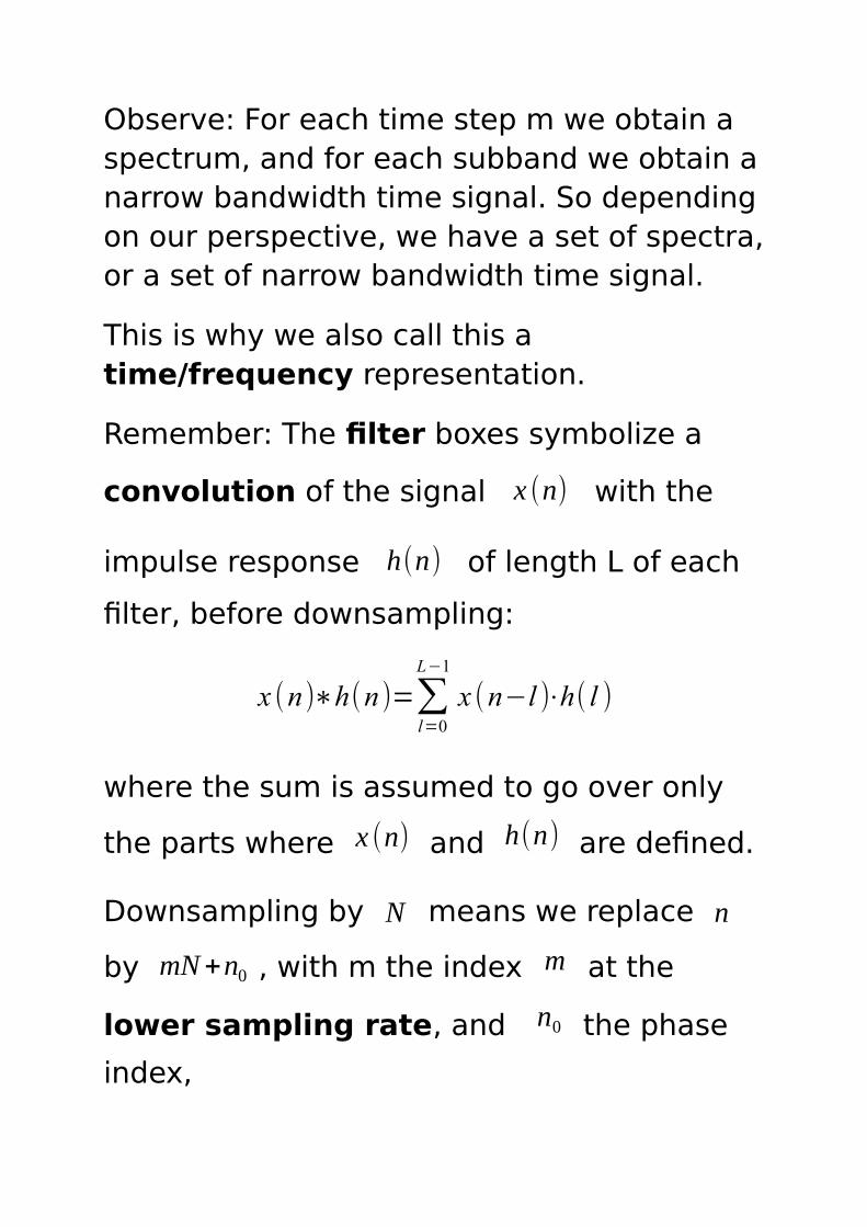
Observe: For each time step m we obtain a spectrum, and for each subband we obtain anarrow bandwidth time signal. So dependingon our perspective, we have a set of spectra,or a set of narrow bandwidth time signal.

This is why we also call this a time/frequency representation.

Remember: The filter boxes symbolize a

convolution of the signal x (n) with the

impulse response h(n) of length L of each

filter, before downsampling:

x (n)∗h(n )=∑l=0

L−1

x (n−l )⋅h( l )

where the sum is assumed to go over only

the parts where x (n) and h(n) are defined.

Downsampling by N means we replace n

by mN+n0 , with m the index m at the

lower sampling rate, and n0 the phase

index,

yn0

↓N (m)=∑n=0

L−1

x(mN+n0−n)hk (n)

The analysis filter bank decomposes the signal into different frequency bands. Observe that each frequency band has a lower sampling rate, which is possible because they have a lower bandwidth. Usingthe “bandpass Nyquist” theorem we can reconstruct the original signal from the subbands!

To reconstruct the original from the different frequency bands, we need the synthesis filter bank:

To simplify notation we dropped the downarrow and phase index for the subband

signals yk(m) .

Observe: The filters after the up-sampling take on the role of the lowpassfilter in the conventional Nyquist theorem, to block the alias components. They “fish out” the correct frequency image out of the aliased images for that subband. All the subbands are then

Rec.

Signal

N

.

.

.

+

N

N

yN−1(m)

y0(m)

x̂ (n)

g0(n)

gN−2(n)

gN−1(n)

xk (n):= y0, k↑N (n)∗gk (n)=∑

n '=0

L−1

y0,k↑N (n−n' )⋅gk (n' )

x̂ (n)=∑k=0

N−1

xk (n)

added up to reconstruct the original signal.

Example for our 2-band system: We have N=2, original sampling rate 32 kHz. Then the low pass branch corresponds to our low pass example above, which reconstructs the signal from 0 to 8 kHz. We now also have a high pass branch, which in addition reconstructs the frequency from 8kHz to 16 kHz. We add the two subbands in the synthesis filter bank to obtain the full bandwidth signal from 0 to 16 kHz.

For the playback of sound (with the function “sound”),

also the software package “sox” needs to be installed

from the software package manager under Linux.

In the command line with

sudo apt-get install sox