Multirate Timestepping Methods

for Hyperbolic Conservation LawsEmil M. Constantinescu and Adrian Sandu

Department of Computer Science, Virginia Polytechnic In-stitute and State University, Blacksburg, VA 24061. E-mail:emconsta, sandu@cs.vt.edu

Abstract

This paper constructs multirate time discretizations for hyperbolic con-servation laws that allow different time-steps to be used in different partsof the spatial domain. The discretization is second order accurate in timeand preserves the conservation and stability properties under local CFLconditions. Multirate timestepping avoids the necessity to take small globaltime-steps (restricted by the largest value of the Courant number on the grid)and therefore results in more efficient algorithms.

1 Introduction

Hyperbolic conservation laws are of great practical importance as they model diversephysical phenomena that appear in mechanical and chemical engineering, aeronautics,astrophysics, meteorology and oceanography, financial modeling, environmental sciences,etc. Representative examples are gas dynamics, shallow water flow, groundwater flow,non-Newtonian flows, traffic flows, advection and dispersion of contaminants, etc.

Conservative high resolution methods with explicit time discretization have gainedwidespread popularity to numerically solve these problems. Stability requirements limitthe temporal step size, with the upper bound being determined by the ratio of the meshspacing and the magnitude of the wave speed. Local spatial refinement reduces theallowable time-step for the explicit time discretizations. The time-step for the entiredomain is restricted by the finest mesh patch or by the highest wave velocity, and istypically (much) smaller than necessary for other variables in the computational domain.

One possibility to circumvent this restriction is to use implicit, unconditionally stabletimestepping algorithms which allow large global time-steps. However, this approachrequires the solution of large (nonlinear) systems of equations. Moreover, the qualityof the solution, as given by a maximum principle, may not be conserved with implicitschemes unless the time-step is restricted by a CFL-like condition.

In this work we seek to develop multirate time integration schemes for the simula-tion of PDEs. In this approach, the time-step can vary spatially and has to satisfy theCFL condition only locally, resulting in substantially more efficient computations. Theapproach follows the method of lines (MOL) framework, where the temporal and spatialdiscretizations are independent.

The development of multirate integration is challenging due to the conservation andstability constraints which timestepping schemes need to satisfy. The algorithms used inthe solution of conservation laws need to preserve the system invariants. Moreover, thesolutions to hyperbolic PDEs may not be smooth: Shock waves or other discontinuousbehavior can develop even from smooth initial data. In such cases, strong-stability-preserving (SSP) numerical methods which satisfy nonlinear stability requirements arenecessary to avoid nonphysical behavior (spurious oscillations, etc.)

A zooming technique for wind transport of air pollution discussed in [Berkvens et al.,1999] is a positive, conservative finite volume discretization that allows the use of smallertime-steps in the region of fine grid resolution. The flux at the coarse-to-fine interface isapplied in the very first fine sub-step in order to preserve positivity.

Dawson and Kirby [Dawson and Kirby, 2001; Kirby, 2002] developed second orderlocal timestepping. The maximum principle, TVD property, and entropy condition are allfulfilled by the second order finite volume method with two level timestepping; however,the timestepping accuracy of the overall method is first order. Tang and Warnecke [2003]reformulated Dawson and Kirby’s algorithm in terms of solution increments to obtainsecond order consistency in time for two-rate integration.

In this paper we develop a general systematic approach to extend Runge-Kutta (RK)to multirate (variable step size) Runge-Kutta methods that inherit the strong stabilityproperties of the corresponding single rate integrators. Additionally, the order of accuracyof the overall scheme is preserved, unlike previous multirate approaches that lead to firstorder accuracy due to the interface treatment [Kirby, 2002; Berkvens et al., 1999]. Moreover,for conservative laws, we show that this multirate approach preserves the linear invariants(i.e. is also conservative).

This paper is structured as follows: In Section 2 we review the main properties andissues of modeling hyperbolic conservation laws. Section 3 presents the construction ofthe multirate time integrators from single rate integrators. Our numerical results withtwo types of conservation laws are shown and discussed in Section 4. Conclusions andfuture research directions are given in Section 5.

2 Hyperbolic Conservation Laws

We consider the following generic one-dimensional scalar hyperbolic equation

∂y(t, x)

∂t+∂ f

(y(t, x)

)

∂x= 0, with y(0, x) = y0(x), (1)

on x ∈ Ω0 ⊂ (−∞, ∞), t > 0 .

The space discretization is usually applied to the equation in conservative form. In theone dimensional finite volume approach, the change in the mean quantity in the ith cell

2

depends on the fluxes through the cell boundaries at i± 12. The semi-discrete (MOL) finite

volume approximation can be written as

y′i = −1

∆x

(Fi+ 1

2− Fi− 1

2

), yi(t) =

1

∆xi

∫ xi+ 1

2

xi− 1

2

y(t, x) dx , y′i =∂yi

∂t, (2)

where ∆xi = xi+ 12− xi− 1

2, (xi = x(i)) is the grid spacing, and Fi+ 1

2= F(xi+k−1, . . . , xi−k) is the

numerical flux at the control volume face.Exact solutions of hyperbolic problems have a range-diminishing property that forbids

existing maxima from increasing, existing minima from decreasing, and new maxima orminima from forming. To provide physically meaningful solutions and avoid weak non-linear instabilities (spurious oscillations), the numerical solution has to satisfy a stabilitycondition. The following are some properties of the numerical solution of conservationlaws that define the stability of the scheme in some sense and are used throughout thispaper.

Maximum principle. Exact solutions of hyperbolic problems have a range-diminishingproperty that forbids existing maxima from increasing, existing minima from decreasing,and new maxima or minima from forming. Formally, it can be written as

max(y(t > 0, x)

)≤ max

(y(t = 0, x)

). (3)

TVD. A numerical method that is called total variation diminishing (TVD) [Harten,1997] if

‖y(t + ∆t, x)‖ ≤ ‖y(t, x)‖ , ‖y‖ =∑

i∈Ω0

|yi+1 − yi| , (4)

where ‖‖ is the total variation semi-norm. No spurious spatial oscillations are introducedduring time-stepping with TVD methods.

Monotonicity-preservation. Monotonic schemes have the property if y0i= y(t = 0, xi) is

monotonically increasing or decreasing in i, then so is by yni

for all tn. A TVD scheme ismonotonicity-preserving.

Positivity. Solution positivity is a typical requirement in various application (e.g. chem-ical engineering, meteorology, financial modeling, etc.). The semi-discrete scheme (2) ispositive if, whenever the initial (condition or) solution is positive, the solution at all futuretimes t > 0 remains positive. A sufficient condition for the positivity of the semi-discretesystem (2) is

yi(t) = 0 and y j(t) > 0 for ∀ j , i⇒ y′i ≥ 0. (5)

We note that the forward Euler method used for time integration maintains all theabove stability properties; however, it has strong CFL restrictions and is only first order

3

accurate. In this paper we use combinations of forward Euler methods in order to preservethe stability properties while increasing the order of accuracy and alleviating the CFLrestrictions.

Several methods that approximate the fluxes in (2) have been developed in the pastdecades. Godunov’s method [Godunov, 1959] is based on the exact solution of Riemannproblems. The flux-corrected transport method proposed by Boris and Book [1997] andfurther developed by Zalesak [1979] and Roe [1981] established the basic principles for theconstruction of high resolution methods. Upwind biased interpolation is coupled withlimiters [Sweby, 1984] which reduce the order of accuracy of the scheme near discontinu-ities (e.g., reducing a high order interpolant to first order, and further limiting its slope).Limiters allow the construction of TVD schemes [Harten, 1997] for nonlinear scalar onedimensional problems.

All these spatial discretization methods satisfy some of the stability properties men-tioned above (maximum principle, TVD, monotonicity-preservation, positivity). ExplicitEuler and later convex combinations of explicit Euler methods are used to solve the semi-discrete form (2), which under the CFL-like condition maintains the stability properties ofthe spatial discretization. Implicit methods are linearly stable; however, the nonlinear sta-bility properties restrict the integration time-step to the CFL-like condition. Moreover, theimplicit methods require the solution of (non)linear systems. Considering these aspectsexplicit discretization methods are preferred for the solution of (2). In the next section webriefly review explicit Runge-Kutta methods and their stability properties.

2.1 Explicit Runge-Kutta Methods

The MOL approach applied to (1) yields the semi-discrete problem (2) which needs tobe solved forward in time. An s stage explicit Runge-Kutta method [Hairer et al., 1993a]computes the next step solution y1 (at time t1 = t0 + ∆t) from the current solution y0 at t0

using the formula:

y1 = y0 + ∆t

s∑

i=1

bi Ki,

Ki = f

t +

i−1∑

j=1

ai j ∆t, y0 + ∆t

i−1∑

j=1

ai j Ki

.

(6)

The method is defined by its coefficients A = ai j, b = bi, and c = ci, which can beconveniently represented in the form of the Butcher tableau [Hairer et al., 1993a]

c1 = 0 0c2 a21

c3 a31 a32...

....... . .

cs as1 as2 · · · as,s−1

b1 b2 · · · bs−1 bs

. (7)

4

All RK methods in this paper consider ci =∑i−1

j=1 ai, j. The order conditions for thesemethods are

Order I :

s∑

i=1

bi = 1 (8)

Order II :

s∑

i=1

s−1∑

j=1

bi ai, j =

s∑

i=1

bi ci =1

2(9)

Next, we discuss some stability properties of Runge-Kutta methods, namely, strongstability preserving.

2.2 Strong Stability Preservation

Strong stability preserving (SSP) integrators are high order timestepping schemes thatpreserve the stability properties of the spatial discretization used with explicit Eulertimestepping. Spurious oscillations (nonlinear instabilities) can occur in a numericalsolution obtained with a TVD or MUSCL spatial discretization scheme, but with a standard(linearly stable) timestepping scheme [Gottlieb et al., 2001]. When TVD discretizationsare combined with SSP timestepping, the numerical solution does not exhibit nonlinearinstabilities. Hence, SSP timestepping schemes are a critical part of the overall solutionstrategy.

The favorable properties of SSP schemes derive from convexity arguments. In particu-lar, if the forward Euler method is strongly stable with a certain CFL number, higher-ordermethods can be constructed as convex combinations of forward Euler steps with variousstep sizes [Shu and Osher, 1988, 1989]. SSP methods preserve the strong stability of theforward Euler scheme for bounded time-steps.

Gottlieb et al. [2001] discuss in detail Runge-Kutta and linear multistep SSP schemes.They derive optimal SSP methods with minimal number of function evaluations, high or-der, low storage, and establish that implicit Runge-Kutta or linear multistep SSP methodsare of order one at most. Hundsdorfer et al. [2003] provide an analysis of monotonicityproperties for linear multistep methods, and Spiteri and Ruuth [2002] extend the SSPRunge-Kutta class of methods.

Several examples of SSP Runge-Kutta are given in [Shu and Osher, 1988], we considera second order method denoted RK2a with its Butcher tableau shown below

0 0 01 1 0

1/2 1/2

K1 = f (y0), yA = y0 + ∆t K1

K2 = f (yA)

y1 = y0 +∆t

2(K1 + K2)

. (10)

Using the following notation to compactly denote Euler steps

E(∆t, y

):= y(t) + ∆t · f (t, y),

5

this method can be written in convex combinations Euler steps, and thus is proven to beSSP by Shu and Osher [1988]:

y1 = y0 +∆t

2(K1 + K2)

=1

2y0 +

1

2yA +

1

2

(yA + ∆t K2

)yA = y0 + ∆t f (y0) = E

(∆t, y0

)

=1

2y0 +

1

2yA +

1

2yA∗ yA∗ = yA + ∆t f (yA) = E

(∆t, yA

)

=y0 + yB

2yB =

yA + yA∗

2=E

(∆t, y0

)+ E

(∆t, yA

)

2(11)

3 Multirate Time Integration

The idea of multirate timestepping is to take different time-steps for different componentsto achieve the target accuracy. The time-steps at different levels need to be synchronizedin order to obtain the desired overall accuracy.

Early efforts to develop multirate Runge-Kutta methods are due to Rice [1960] andAndrus [1979, 1993]. Multirate versions of many of the traditional timestepping schemeshave been proposed in the literature. Such methods include linear multistep [Gear andWells, 1984; Kato and Kataoka, 1999], extrapolation [Engstler and Lubich, 1997], Runge-Kutta [Kværnø and Rentrop, 1999; Kværnø, 2000; Günther et al., 1998], Rosenbrock-Wanner [Günther and Rentrop, 1993; Bartel and Günther, 2002], waveform relaxation[Sand and Burrage, 1998], Galerkin [Logg, 2003a,b, 2006, 2004], and combined multi-scaleapproaches [Engquist and Tsai, 2005]. For the majority of methods, slower componentsare integrated using larger step sizes, integer multiples of the smaller step sizes used forfast components,∆tslow = m∆tfast. All steps are synchronized every largest time-step∆tslow.Conditions for high orders of accuracy for the multirate integrators (at the synchronizationtimes) are derived in the literature.

Kværnø and Rentrop [1999]; Kværnø [2000] developed multirate Runge Kutta (MRK)methods where the coupling between slow and fast components is done by intermediatestage values. Günther et al. [1998] developed multirate partitioned Runge-Kutta (MPRK)schemes which generalize both partitioned Runge-Kutta and multirate ROW methods[Günther and Hoschek, 1997], and Sand et. al. developed the Jacobi waveform relaxationapproach [Sand and Burrage, 1998].

For the purpose, of simplicity without the loss of generality, in the following sections werestrict our discussion to scalar one dimensional equations. Multidimensional/multivariableextensions are straightforward.

Consider the system of ordinary differential equations in (2) resulting from the appli-cation of MOL to (1) where a partitioning of variables according to their characteristictimes is possible:

y =[y1, · · · , yM

]T , y′i = fi

(t, y1, · · · , yM

), i = 1, · · · ,M . (12)

6

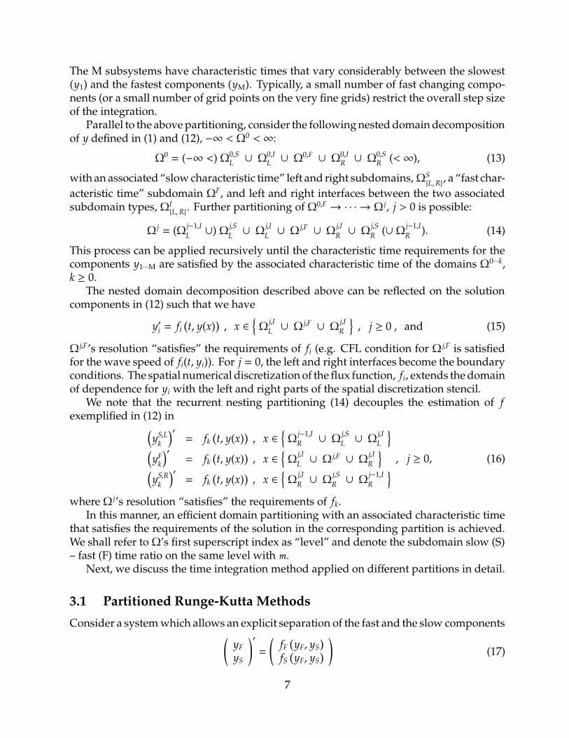
The M subsystems have characteristic times that vary considerably between the slowest(y1) and the fastest components (yM). Typically, a small number of fast changing compo-nents (or a small number of grid points on the very fine grids) restrict the overall step sizeof the integration.

Parallel to the above partitioning, consider the following nested domain decompositionof y defined in (1) and (12), −∞ < Ω0 < ∞:

Ω0 = (−∞ <) Ω0,SL∪ Ω0,I

L∪ Ω0,F ∪ Ω0,I

R∪ Ω0,S

R(< ∞), (13)

with an associated “slow characteristic time” left and right subdomains,ΩSL,R

, a “fast char-

acteristic time” subdomain ΩF, and left and right interfaces between the two associatedsubdomain types, ΩI

L,R. Further partitioning of Ω0,F → · · · → Ω j, j > 0 is possible:

Ω j = (Ωj−1,I

L∪) Ω

j,S

L∪ Ω

j,I

L∪ Ω j,F ∪ Ω

j,I

R∪ Ω

j,S

R(∪ Ω

j−1,I

R). (14)

This process can be applied recursively until the characteristic time requirements for thecomponents y1···M are satisfied by the associated characteristic time of the domains Ω0···k,k ≥ 0.

The nested domain decomposition described above can be reflected on the solutioncomponents in (12) such that we have

y′i = fi

(t, y(x)

), x ∈

Ω

j,I

L∪ Ω j,F ∪ Ω

j,I

R

, j ≥ 0 , and (15)

Ω j,F’s resolution “satisfies” the requirements of fi (e.g. CFL condition for Ω j,F is satisfiedfor the wave speed of fi(t, yi)). For j = 0, the left and right interfaces become the boundaryconditions. The spatial numerical discretization of the flux function, fi, extends the domainof dependence for yi with the left and right parts of the spatial discretization stencil.

We note that the recurrent nesting partitioning (14) decouples the estimation of fexemplified in (12) in

(yS,L

k

)′= fk

(t, y(x)

), x ∈

Ω

j−1,I

R∪ Ω

j,S

L∪ Ω

j,I

L

(yF

k

)′= fk

(t, y(x)

), x ∈

Ω

j,I

L∪ Ω j,F ∪ Ω

j,I

R

(yS,R

k

)′= fk

(t, y(x)

), x ∈

Ω

j,I

R∪ Ω

j,S

R∪ Ω

j−1,I

R

, j ≥ 0, (16)

where Ω j’s resolution “satisfies” the requirements of fk.In this manner, an efficient domain partitioning with an associated characteristic time

that satisfies the requirements of the solution in the corresponding partition is achieved.We shall refer to Ω’s first superscript index as “level” and denote the subdomain slow (S)– fast (F) time ratio on the same level with m .

Next, we discuss the time integration method applied on different partitions in detail.

3.1 Partitioned Runge-Kutta Methods

Consider a system which allows an explicit separation of the fast and the slow components(

yF

yS

)′=

(fF

(yF, yS

)

fS

(yF, yS

))

(17)

7

Partitioned Runge-Kutta (PRK) methods [Hairer et al., 1993b; Hairer, 1981] are used to

solve the problem (17) with two different methods, RK F=

[AF, bF, cF

]for the fast part,

and RK S=

[AS, bS, cS

]for the slow part. The coefficients of these methods are AF = aF

i j,

bF, cF, and AS = aSi j, bS, cS. The PRK solution method reads [Hairer et al., 1993b; Hairer,

1981]

y1F = y0

F + ∆t

S∑

i=1

bFi K

j

F, y1

S = y0S + ∆t

S∑

i=1

bSi K

j

S

YiF = y0

F + ∆t

S∑

j=1

aFi jK

j

F, Yi

S = y0S + ∆t

S∑

j=1

aSi jK

j

S(18)

KiF = fF

(Yi

F ,YiS

), Ki

S = fS

(Yi

F ,YiS

).

The order of the coupled method is the minimum order among each method taken sepa-rately and the order of the “coupling”. The first order coupling conditions are implicitlysatisfied. The second order coupling conditions are

s∑

i=1

bFi cS

i =1

2

s∑

i=1

bSi cF

i =1

2. (19)

There are over 20 third order coupling conditions that can be found in [Hairer et al., 1993b].Here, we list just two that will be used later in this paper

s∑

i=1

bFi cF

i cSi =

1

6

s∑

i=1

bSi cS

i cFi =

1

6. (20)

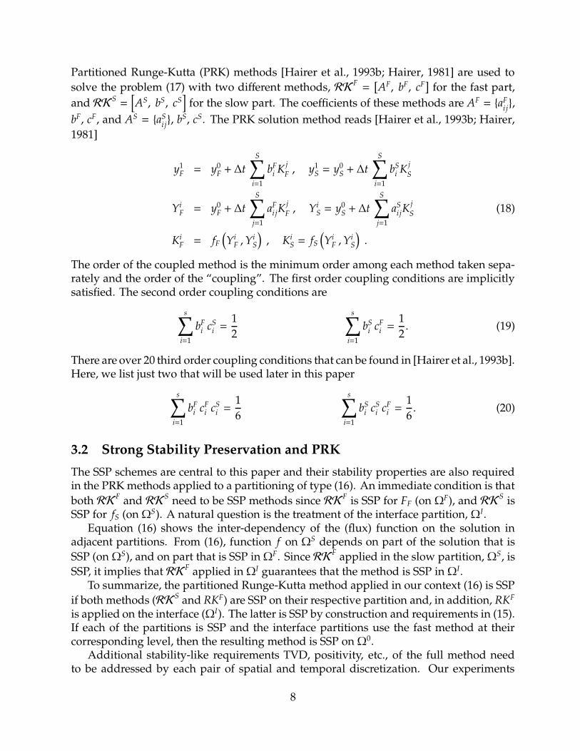
3.2 Strong Stability Preservation and PRK

The SSP schemes are central to this paper and their stability properties are also requiredin the PRK methods applied to a partitioning of type (16). An immediate condition is that

both RK F and RKS need to be SSP methods since RKF is SSP for FF (on ΩF), and RK S isSSP for fS (on ΩS). A natural question is the treatment of the interface partition, ΩI.

Equation (16) shows the inter-dependency of the (flux) function on the solution inadjacent partitions. From (16), function f on ΩS depends on part of the solution that is

SSP (on ΩS), and on part that is SSP inΩF. Since RKF applied in the slow partition, ΩS, is

SSP, it implies that RK F applied in ΩI guarantees that the method is SSP in ΩI.To summarize, the partitioned Runge-Kutta method applied in our context (16) is SSP

if both methods (RK S and RKF) are SSP on their respective partition and, in addition, RKF

is applied on the interface (ΩI). The latter is SSP by construction and requirements in (15).If each of the partitions is SSP and the interface partitions use the fast method at theircorresponding level, then the resulting method is SSP on Ω0.

Additional stability-like requirements TVD, positivity, etc., of the full method needto be addressed by each pair of spatial and temporal discretization. Our experiments

8

RKB

RKF

RKS

c Ab

1m c 1

m A

1m

+ 1

m c 1m

bT 1

m A

......

. . .

m−1m

+ 1

m c 1m

bT · · · 1

m

bT 1

m A

1m b 1

m b . . . 1m b

c A

c A

.... . .

c A

1m b 1

m b . . . 1m b

(a) Base (b) Fast method (c) Slow method

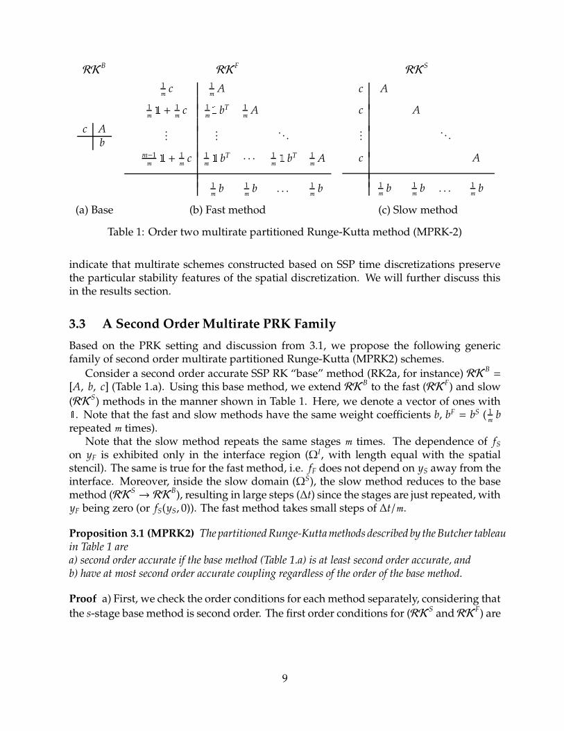
Table 1: Order two multirate partitioned Runge-Kutta method (MPRK-2)

indicate that multirate schemes constructed based on SSP time discretizations preservethe particular stability features of the spatial discretization. We will further discuss thisin the results section.

3.3 A Second Order Multirate PRK Family

Based on the PRK setting and discussion from 3.1, we propose the following genericfamily of second order multirate partitioned Runge-Kutta (MPRK2) schemes.

Consider a second order accurate SSP RK “base” method (RK2a, for instance) RK B=

[A, b, c] (Table 1.a). Using this base method, we extend RK B to the fast (RKF) and slow

(RKS) methods in the manner shown in Table 1. Here, we denote a vector of ones with. Note that the fast and slow methods have the same weight coefficients b, bF = bS ( 1

m brepeated m times).

Note that the slow method repeats the same stages m times. The dependence of fS

on yF is exhibited only in the interface region (ΩI, with length equal with the spatialstencil). The same is true for the fast method, i.e. fF does not depend on yS away from theinterface. Moreover, inside the slow domain (ΩS), the slow method reduces to the basemethod (RKS

→ RKB), resulting in large steps (∆t) since the stages are just repeated, with

yF being zero (or fS(yS, 0)). The fast method takes small steps of ∆t/m .

Proposition 3.1 (MPRK2) The partitioned Runge-Kutta methods described by the Butcher tableauin Table 1 area) second order accurate if the base method (Table 1.a) is at least second order accurate, andb) have at most second order accurate coupling regardless of the order of the base method.

Proof a) First, we check the order conditions for each method separately, considering that

the s-stage base method is second order. The first order conditions for (RK S andRK F) are

9

verified since by (8) we have

m×s∑

i=1

bSi = m

s∑

j=1

bi = 1

m×s∑

i=1

bFi = m

s∑

j=1

bi = 1.

The second order conditions (9) are also satisfied

m×s∑

i=1

bSi cS

i =1

m

s∑

i=1

biT ci =

1

mm2=

1

2,

and for RK F we have

m×s∑

i=1

bFi cF

i =1

m2

(bTc + bT (

+ c) + · · · + bT ((m − 1)

+ c)

)

=1

m2

m2+

m∑

i=1

m

=1

m2

(m2+

m(m − 1)

2

)

=1

2

Since bF = bS, the coupling conditions (19) are satisfied directly by the above. Hence,MPRK2 is at least second order accurate.b) Consider that RKB satisfies the third order accuracy conditions, then the third ordercoupling condition (20) requires the following

bTFcFcS = bT

F

[12c2

12

(c + c2

)]

=1

4bTc2 +

1

4

(bTc + bTc2

)

=1

4·

1

3+

1

4

(1

2+

1

3

)

=7

24,

1

6,

and thus, (at the interface) the method reduces to second order coupling accuracy.

The method presented in this section represents a truly multirate approach since thefast method takes m successive steps of the base method with a time-step of ∆t/m . Thismethod can be easily extended from m = 2 to m = 3. In Appendix B we present the samemethod for m = 3.

In order to increase the coupling order, we need to investigate other schemes thathave a different layout (perhaps using different base methods for the fast and for the slowsubsystems). Such methods will be investigated in future studies.

10

Proposition 3.2 (Conservation) The partitioned Runge-Kutta methods described by the Butchertableau in Table 1 preserve the linear invariants of the system.

Proof This is a direct consequence of having chosen equal weights for the fast and for theslow methods, bF = bS. Consider the system (17) with a linear invariant of the form

eF fF

(yF, yS

)+ eS fS

(yF, yS

)= 0 ∀yF, yS ⇒ eFyF(t) + eSyS(t) = const ∀t ,

where eF, eS are fixed weight vectors.From the method (18) with bF = bS = b∗ we have that

y1F = y0

F + ∆t

S∑

i=1

b∗i fF

(Yi

F ,YiS

), y1

S = y0S + ∆t

S∑

i=1

b∗i fS

(Yi

F ,YiS

)

and therefore

eFy1F + eSy1

S = eFy0F + eSy0

S + ∆t

S∑

i=1

b∗i

(eF fF

(Yi

F ,YiS

)+ eS fS

(Yi

F ,YiS

)

︸ ︷︷ ︸0

)= eFy0

F + eSy0S .

This property is important because multirate Runge-Kutta methods, used in conjunc-tion with conservative space discretizations, lead to conservative full discretizations of thePDE. For example, consider a one-dimensional finite volume scheme in the conservativeformulation:

y′i =1

∆xi

(Fi− 1

2(y) − Fi+ 1

2(y)

), 1 ≤ i ≤ N .

where Fi+ 12

is the numerical flux through the i + 12

interface. Assuming no fluxes throughthe leftmost and the rightmost boundaries (F 1

2= FN+ 1

2= 0), the finite volume discretization

is conservative in the sense that

N∑

i=1

∆xi y′i = 0 ,N∑

i=1

∆xi yi = const .

The time discretization with a classical (single-rate) Runge Kutta method gives a conserva-tive fully discrete method. We want to show that the multirate method is also conservative.For this, assume that the leftmost ` grid cells are the fast domain (yF = y1, · · · , y`), andthe remaining cells are the slow domain yS = y`+1, · · · , yN). Each subdomain is advancedin time with a classical Runge-Kutta method, therefore the fluxes exchanged between theboundaries of same-class cells are conserved. The question remains whether the fluxescrossing the fast-slow interface are conserved. We now show that the total flux lost by thefast domain through the fast-slow interface is exactly the total flux received by the slowdomain through the same interface.

11

0 0 01 1 0

1/2 1/2

0 01/2 1/2 01/2 1/4 1/4 01 1/4 1/4 1/2 0

1/4 1/4 1/4 1/4

0 01 1 00 0 0 01 0 0 1 0

1/4 1/4 1/4 1/4(a) Base method (b) Fast method (c) Slow method

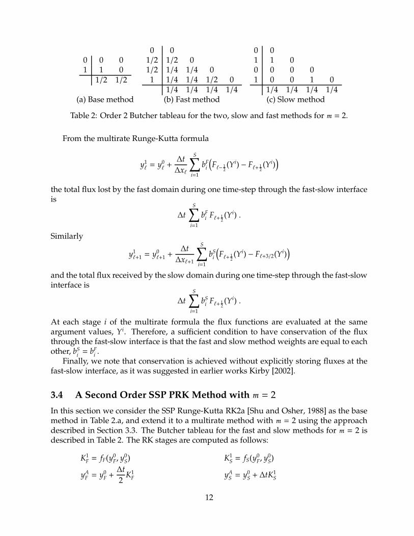
Table 2: Order 2 Butcher tableau for the two, slow and fast methods for m = 2.

From the multirate Runge-Kutta formula

y1` = y0

` +∆t

∆x`

S∑

i=1

bFi

(F`− 1

2(Yi) − F`+ 1

2(Yi)

)

the total flux lost by the fast domain during one time-step through the fast-slow interfaceis

∆t

S∑

i=1

bFi F`+ 1

2(Yi) .

Similarly

y1`+1 = y0

`+1 +∆t

∆x`+1

S∑

i=1

bSi

(F`+ 1

2(Yi) − F`+3/2(Yi)

)

and the total flux received by the slow domain during one time-step through the fast-slowinterface is

∆t

S∑

i=1

bSi F`+ 1

2(Yi) .

At each stage i of the multirate formula the flux functions are evaluated at the sameargument values, Yi. Therefore, a sufficient condition to have conservation of the fluxthrough the fast-slow interface is that the fast and slow method weights are equal to eachother, bS

i= bF

i.

Finally, we note that conservation is achieved without explicitly storing fluxes at thefast-slow interface, as it was suggested in earlier works Kirby [2002].

3.4 A Second Order SSP PRK Method with m = 2

In this section we consider the SSP Runge-Kutta RK2a [Shu and Osher, 1988] as the basemethod in Table 2.a, and extend it to a multirate method with m = 2 using the approachdescribed in Section 3.3. The Butcher tableau for the fast and slow methods for m = 2 isdescribed in Table 2. The RK stages are computed as follows:

K1F = fF(y0

F, y0S) K1

S = fS(y0F, y

0S)

yAF = y0

F +∆t

2K1

F yAS = y0

S + ∆tK1S

12

K2F = fF(yA

F , yAS ) K2

S = fS(yAF , y

AS )

yBF = y0

F +∆t

4K1

F +∆t

4K2

F yBS = y0

S

K3F = fF(yB

F , y0S) K3

S = fS(yBF , y

0S) (21)

yCF = yB

F +∆t

2K3

F yCS = y0

S + ∆tK3S

K4F = fF(yC

F , yCS ) K4

S = fS(yCF , y

CS )

y1F = y0

F +∆t

4

(K1

F + K2F + K3

F + K4F

)y1

S = y0S +∆t

4

(K1

S + K2S + K3

S + K4S

)

Using the following notation to compactly denote Euler steps

EF,S(∆t, yF, yS

):= yF,S(t) + ∆t · fF,S(t, yF, yS), (22)

the above MPRK2 can be written in Euler steps in the following way:

y1F =

1

2

(y0

F + y0F +∆t

2K1

F +∆t

2K2

F +∆t

2K3

F +∆t

2K4

F

), yA

F = EF

(∆t

2, y0

F, y0S

)

=1

2

(y0

F + yAF +∆t

2K2

F +∆t

2K3

F +∆t

2K4

F

), yA∗

F = EF

(∆t

2, yA

F , yAS

)

=1

2

(y0

F + yA∗F +∆t

2K3

F +∆t

2K4

F

), 2yB

F = y0F + yA∗

F yCF = EF

(∆t

2, yB

F, y0S

)

=1

2

(yB

F + yCF +∆t

2K4

F

), yC∗

F = EF

(∆t

2, yC

F , yCS

)

=1

2

(yB

F + yC∗F

), (23)

and

y1S =

1

4

(2y0

S + y0S + ∆tK1

S + ∆tK2S + y0

S + ∆tK3S + ∆tK4

S

), yA,C

S= ES

(∆t, y0,B

F, y0

S

)

=1

4

(2y0

S + yAS + ∆tK2

S + yCS + hK4

S

), yA∗,C∗

S= ES

(∆t, yA,C

F, yA,C

S

)

=1

4

(2y0

S + yA∗S + yC∗

S

). (24)

The Euler steps for the fast and slow methods are summarized in the appendix A inTable 5.

We now asses how this timestepping method preserves the maximum principle andnonlinear stability properties of the discretization. Kirby [2002] has carried out this kindof analysis for the multirate explicit Euler method.

Proposition 3.3 (Positivity) If each fast multirate Euler step

y1F = EF

(∆t

m, y0

F, y0S

)

13

and each slow multirate Euler step

y1S = ES

(∆t, y0

F, y0S

)

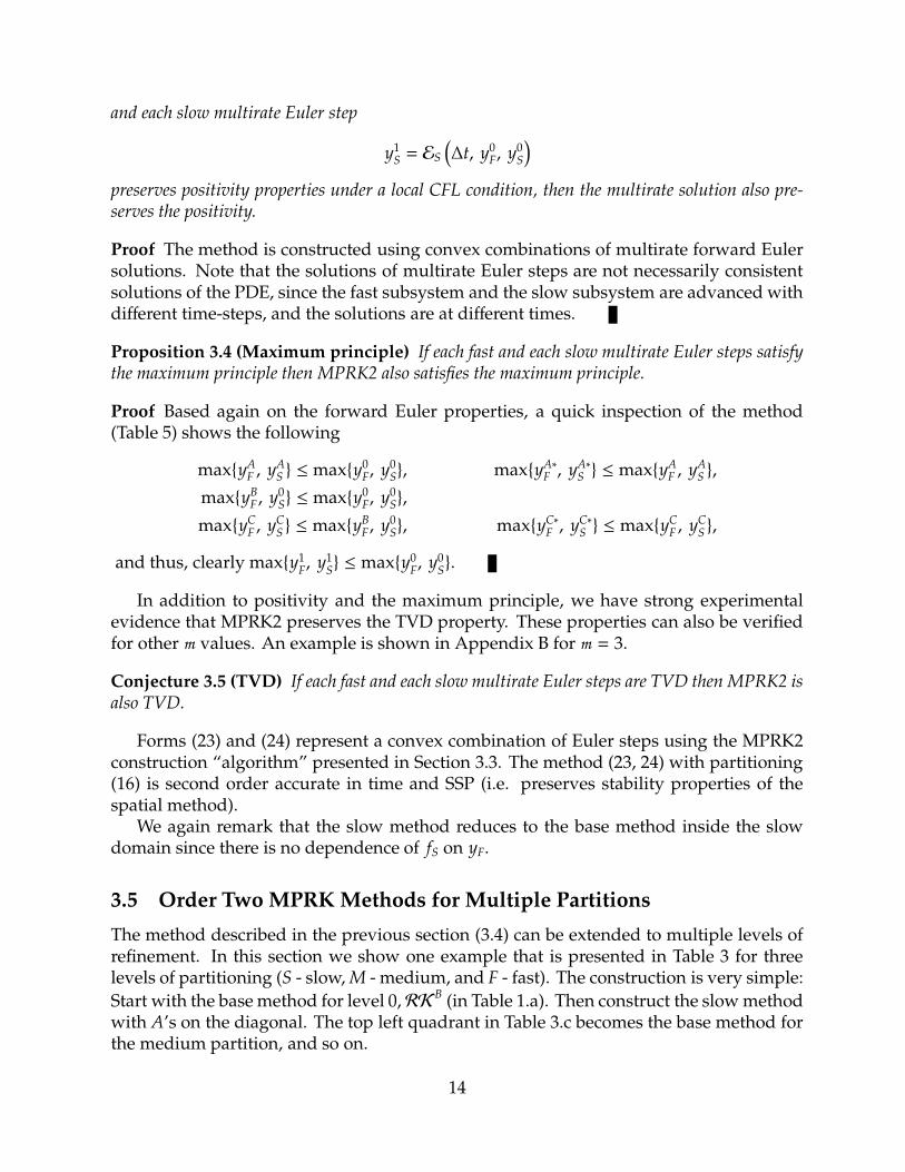
preserves positivity properties under a local CFL condition, then the multirate solution also pre-serves the positivity.

Proof The method is constructed using convex combinations of multirate forward Eulersolutions. Note that the solutions of multirate Euler steps are not necessarily consistentsolutions of the PDE, since the fast subsystem and the slow subsystem are advanced withdifferent time-steps, and the solutions are at different times.

Proposition 3.4 (Maximum principle) If each fast and each slow multirate Euler steps satisfythe maximum principle then MPRK2 also satisfies the maximum principle.

Proof Based again on the forward Euler properties, a quick inspection of the method(Table 5) shows the following

maxyAF , yA

S ≤ maxy0F, y0

S, maxyA∗F , yA∗

S ≤ maxyAF , yA

S ,

maxyBF , y0

S ≤ maxy0F, y0

S,

maxyCF , yC

S ≤ maxyBF, y0

S, maxyC∗F , yC∗

S ≤ maxyCF , yC

S ,

and thus, clearly maxy1F, y1

S ≤ maxy0

F, y0

S.

In addition to positivity and the maximum principle, we have strong experimentalevidence that MPRK2 preserves the TVD property. These properties can also be verifiedfor other m values. An example is shown in Appendix B for m = 3.

Conjecture 3.5 (TVD) If each fast and each slow multirate Euler steps are TVD then MPRK2 isalso TVD.

Forms (23) and (24) represent a convex combination of Euler steps using the MPRK2construction “algorithm” presented in Section 3.3. The method (23, 24) with partitioning(16) is second order accurate in time and SSP (i.e. preserves stability properties of thespatial method).

We again remark that the slow method reduces to the base method inside the slowdomain since there is no dependence of fS on yF.

3.5 Order Two MPRK Methods for Multiple Partitions

The method described in the previous section (3.4) can be extended to multiple levels ofrefinement. In this section we show one example that is presented in Table 3 for threelevels of partitioning (S - slow, M - medium, and F - fast). The construction is very simple:

Start with the base method for level 0,RKB (in Table 1.a). Then construct the slow methodwith A’s on the diagonal. The top left quadrant in Table 3.c becomes the base method forthe medium partition, and so on.

14

X[RK

F0

] [RK

S0

]

[RK

F1

] [RK

S1

]X

14

c 14

A+c4

14

b 14

A

2·+c

414

b 14

b 14

A

3·+c

414

b 14

b 14

b 14

A

14

b 14

b 14

b 14

b

c2

12

A

c2

12

A

+c2

14

b 14

b 12

A+c2

14

b 14

b 12

A

14

b 14

b 14

b 14

b

c A

c A

c A

c A

14

b 14

b 14

b 14

b

(a) Fast method (m = 4) (b) Medium method (m = 2) (c) Slow method (m = 1)

Table 3: Multirate partitioned Runge-Kutta method (MPRK2) with 3 levels of refinement

For multiple levels, each method depends on its corresponding partition and only onthe neighboring (left/right) partitions. In this case, the dependency of fF,M,S on yF,M,S isthe following

y′F = fF(yF, yM)

y′M = fM(yF, yM, yS)

y′S= fS(yM, yS)

.

We note that there is no direct dependency between flux functions fF and fS. The transitionbetween the fast and the slow methods is smoothly resolved in this context.

Clearly, the order conditions for each method and for the coupling are satisfied. More-

over, on level 0, RKS0 reduces to the base method on Ω0,S (away from the interface), and

in turn, RKS1 reduces to the top left quadrant of RK S

0 on Ω1,S, which becomes the basemethod for the medium partition. Thus, we have a clear and systematic way to expandmethods on increasingly faster partitions.

As stated before in this paper, from the efficiency stand point, there is no additionalcomputational load away from the interface regions which are typically very small com-pared to the fast and slow partitions.

4 Numerical Results

We consider two standard test problems: the advection equation and the simplified(inviscid) Burgers’ equation. Since TVD methods in multiple dimensions are at mostfirst order accurate [Goodman et al., 1985], we look at one dimensional problems. Veryaccurate multiple dimension problems can be implemented using dimension splitting.The solutions are computed using a method of lines approach. The linear advection spatialdiscretization is a second order limited finite volume scheme on nonuniform grids that

15

is both conservative and positive (described in Section 4.1). Burgers’ equation, describedin Section 4.2, is implemented on a fixed grid, using a third order scheme developed byOsher and Chakravarthy [1986].

4.1 The Advection Equation

The one-dimensional advection equation (25) models the transport of a tracer y with theconstant velocity u along the x axis.

∂y(t, x)

∂t+ u ·

∂y(t, x)

∂x= 0 . (25)

4.1.1 Positive Spatial Discretization

In what follows, we describe the positive (5) flux limited spatial discretization scheme[Hundsdorfer et al., 1995; Vreugdenhil and Koren, 1993]. We start by introducing the fluxlimited formulation of Hundsdorfer et al. [1995] on uniform grids, and extend the schemeto nonuniform grids.

The numerical flux can be defined as

Fi+ 12= fi +

1

2φi+ 1

2

(fi − fi−1

), (26)

where φ is a nonlinear function called limiter. Then scheme (2) can be written as

∂

∂tyi = −

(1 + 1

2φi+ 1

2

) (fi − fi−1

)− 1

2φi− 1

2

(fi−1 − fi−2

)

∆x. (27)

Define the flux slope ratio

ri− 12=

fi − fi−1

fi−1 − fi−2

, (28)

If we consider ri− 12, 0, from (27) and (28) we have

∂

∂tui = −

1

∆x

(1 +

1

2φi+ 1

2

)−

12φi− 1

2

ri− 12

(

fi − fi−1

). (29)

The positivity requirement (5) applied to the scheme (29) yields the following condition

φi− 12

ri− 12

− φi+ 12≤ 2. (30)

This condition is used to impose bounds on the limiter φ for the numerical flux definedby (26) in order to preserve positivity for the scheme (2).

Now, we extend the scheme and the limiter to a nonuniform grid by redefining thenumerical flux. Consider a quadratic (spatial) flux interpolant for the numerical flux

16

function F at i + 12, using the flux function f , evaluated at gridpoints i − 1, i, i + 1, and a

nonuniform spatial grid spacing, ∆x[], in the following form:

Fi+ 12= fi + αi fi−1 + βi fi + γi fi+1,

where

αi = −∆xi ∆xi+1

(∆xi−1 + ∆xi) (∆xi+1 + 2∆xi + ∆xi−1)

βi = −∆xi (∆xi−1 + ∆xi − ∆x1+i)

(∆xi−1 + ∆xi) (∆xi + ∆xi+1)

γi =∆xi (∆xi−1 + 2∆xi)

(∆xi + ∆xi+1) (∆xi+1 + 2∆xi + ∆xi−1), with

αi + βi + γi = 0.

The flux can be written in terms of(

fi − fi−1

)and r as

Fi+ 12= fi +

(−αi + γi ri+ 1

2

) (fi − fi−1

). (31)

DefineK as

K (r) = 2(−αi + γi r

). (32)

Then, the numerical flux can be expressed as

Fi+ 12= fi +

1

2K

(ri+ 1

2

) (fi − fi−1

). (33)

Just as in [Hundsdorfer et al., 1995; Sweby, 1984], we define the following flux limiter

φ(r) = max(0, min

(2 r, min

(δ, K 2 (r)

))), (34)

and take δ = 2.The semi-discrete form (2) with the limiter (34) using the numerical flux defined by

(33) is a positive, second order (wherever the limiter is set to one) semi-discrete schemeon a nonuniform grid. The proofs follow immediately from [Hundsdorfer et al., 1995;Sweby, 1984] with the extension of the nonuniform mesh. In addition, if the timesteppingscheme is positivity preserving, then the entire method (each multirate step, in our case)is positivity preserving.

Figure 1 shows the leading order truncation error of the spatial discretization usingthe unlimited numerical flux (31), i.e. the coefficient that multiplies ∂ f

′′′

/∂3x.

4.1.2 Numerical Experiments

In this section we show a few examples and instances of MPRK2 schemes for the linearadvection equation that clearly show one of their applications and potential. The spatial

17

Coarse Fine Coarse−10

−5

0

5

10

15

Tru

nc. C

oeff.

× 1/

48

∆ xfine

= ∆ xcoarse

= ∆ x

∆ xfine

= ∆ xcoarse

= 2 ∆ x

2 ∆ xfine

= ∆ xcoarse

Coarse Fine Coarse−20

−10

0

10

20

30

40

Tru

nc. C

oeff.

× 1/

48

∆ xfine

= ∆ xcoarse

= ∆ x

∆ xfine

= ∆ xcoarse

= 3 ∆ x

3 ∆ xfine

= ∆ xcoarse

(a) m = 2 (b) m = 3

Figure 1: Representation of the discretization leading order error term for two instancesof m as the wave passes through the interfaces.

discretization is positive and the time integration scheme is SSP, which results in an overallpositive scheme.

Our test cases include three different function shapes (ordered by their regularity): astep function, a triangular shape, and an exponential shape.

The computational domain has three distinct regions. The middle region is discretizedusing a fine grid with spacing ∆x/m , while the left and right regions are covered by acoarse mesh with spacing ∆x. For simplicity we consider periodic boundary conditions.The timestepping interval is proportional with the grid size in order to satisfy the CFLrestriction, i.e. we take ∆t wherever we have ∆x grid spacing and ∆t/m wherever we have∆x/m .

Figures 2 show the advection equation with the three function profiles that passthrough a fixed fine (∆x/m) region (located between x = 1 and x = 2). The dashedline represents the exact solution and solid line corresponds to the solution evolved withunit wave speed (u = 1) in time (at two different time indices). Here, we see that thesolution is not qualitatively affected by the interface. Moreover, with the higher spa-tial resolution, the solution improves qualitatively (as m is larger), and the wave is notdistorted by passing through the interface.

To quantify the benefits of having a finer region in this setting, we investigate a movingfine mesh that is centered around the “interesting region,” where the large gradients occurin the solution. Figures 3 show the advection equation with the three corresponding initialfunction profiles (marked with dashed lines) located on the right part of the domain ona fine (∆x/m) mesh. The initial profile is advected with unit wave speed (to the left partof the domain). The Figures show the final state of the solution with the exact solutionsuperimposed (marked with dotted lines), and the vertical dotted lines delimit the finedomain. Table 4 shows the L1 error norm of the moving for the profiles shown in Figures 3.Clearly, the solution is improved both qualitatively and quantitatively with higher spatialresolution.

All the results for the advection equation presented in this section show that this

18

0 0.5 1 1.5 2 2.50

0.2

0.4

0.6

0.8

1

0 0.5 1 1.5 2 2.50

0.2

0.4

0.6

0.8

1

0 0.5 1 1.5 2 2.50

0.2

0.4

0.6

0.8

1

(a) RK2a (m = 1) (b) MPRK2, m = 2 (c) MPRK2, m = 3

0 0.5 1 1.5 2 2.50

0.2

0.4

0.6

0.8

1

0 0.5 1 1.5 2 2.50

0.2

0.4

0.6

0.8

1

0 0.5 1 1.5 2 2.50

0.2

0.4

0.6

0.8

1

(d) RK2a (m = 1) (e) MPRK2, m = 2 (f) MPRK2, m = 3

0 0.5 1 1.5 2 2.50

0.2

0.4

0.6

0.8

1

0 0.5 1 1.5 2 2.50

0.2

0.4

0.6

0.8

1

0 0.5 1 1.5 2 2.50

0.2

0.4

0.6

0.8

1

(g) RK2a (m = 1) (h) MPRK2, m = 2 (i) MPRK2, m = 3

Figure 2: Fixed grid advection equation with three function profiles that pass through afixed fine (∆x/m , ∆t/m) region (between 1 and 2). The dashed line represents the exactsolution and solid line corresponds to the solution evolved in time (at two different timeindices)

Type m = 1 m = 2 m = 3Step 0.1085 0.1069 0.1021Triangular 0.0401 0.0224 0.0154Exponential 0.0466 0.0344 0.0270

Table 4: L1 error norm of the moving grid advection equation.

19

0 0.5 1 1.5 2 2.50

0.2

0.4

0.6

0.8

1

0 0.5 1 1.5 2 2.50

0.2

0.4

0.6

0.8

1

0 0.5 1 1.5 2 2.50

0.2

0.4

0.6

0.8

1

(a) RK2a (m = 1) (b) MPRK2, m = 2 (c) MPRK2, m = 3

0 0.5 1 1.5 2 2.50

0.2

0.4

0.6

0.8

1

0 0.5 1 1.5 2 2.50

0.2

0.4

0.6

0.8

1

0 0.5 1 1.5 2 2.50

0.2

0.4

0.6

0.8

1

(d) RK2a (m = 1) (e) MPRK2, m = 2 (f) MPRK2, m = 3

0 0.5 1 1.5 2 2.50

0.2

0.4

0.6

0.8

1

0 0.5 1 1.5 2 2.50

0.2

0.4

0.6

0.8

1

0 0.5 1 1.5 2 2.50

0.2

0.4

0.6

0.8

1

(g) RK2a (m = 1) (h) MPRK2, m = 2 (i) MPRK2, m = 3

Figure 3: Moving grid advection equation with three function profiles (initially markedwith dashed lines) that pass through a fixed fine (∆x/m , ∆t/m) region (between x = 1 andx = 2). The dotted line represents the exact solution and solid line corresponds to thesolution evolved in time.

specific finite volume approach and MPRK2 yield a multirate solution on a nonuniformgrid that is conservative and positive, as discussed in Section 3.4.

4.2 Burgers’ equation

The simplified inviscid Burgers equation is described by

∂y(t, x)

∂t+∂

∂x

(1

2y(t, x)2

)= 0 (35)

20

Burgers’ equation numerical experiments are based on the third order upwind-biased TVDflux limited scheme described below.

4.2.1 TVD Spatial Discretization

This section is based on the work of Osher and Chakravarthy [1984, 1986]; Chakravarthyand Osher [1983]. A generic recipe for high order TVD finite volume schemes can be foundin [Chakravarthy and Osher, 1985]. In what follows, we briefly present their method.

Consider the flux F(y j+1, y j) to be a scalar numerical flux defined for an E-scheme[Chakravarthy and Osher, 1985]. The following

d f−j+ 1

2

= F(y j+1, y j) − f (y j), and (36)

d f+j+ 1

2

= f (y j+1) − F(y j+1, y j), (37)

represent the positive and negative flux difference on the cell border.With (36, 37), consider the following numerical flux

F j+ 12= F(y j+1, y j) −

[1 − κ

4d f−

j+ 32

+1 + κ

4d f−

j+ 12

]+

[1 + κ

4d f+

j+ 12

+1 − κ

4d f+

j− 12

], (38)

F(y j+1, y j) =1

2

(f (y j+1) + f (y j)

)−

1

2

(d f+

j+ 12

+ d f−j+ 1

2

), (39)

where f ± are the negative and positive flux contributions, d f± and d f ± show that theyare in flux limited form and are defined below. The scheme defined by (38) is called aκ scheme. If κ = 1

3, (38) becomes the limited third order upwind-biased scheme. If we

consider d f ± = d f± and d f± = d f±, we have the unlimited scheme. The limited fluxes aredefined as follows

d f−j+ 3

2

= minmod

[d f−

j+ 32

, b d f −j+ 1

2

], d f−

j+ 12

= minmod

[d f−

j+ 12

, b d f −j+ 3

2

], (40)

d f+j+ 1

2

= minmod

[d f+

j+ 12

, b d f +j− 1

2

], d f+

j− 12

= minmod

[d f+

j− 12

, b d f +j+ 1

2

], (41)

where

minmod[x, y

]= sign(x) ·max

[0, min

[|x|, y sign(x)

]], 1 ≤ b ≤

3 − κ

1 − κ. (42)

The semi-discrete form (2) using the numerical flux defined by (40) is a TVD, third or-der accurate scheme for κ = 1

3(when the limiter is not “active”, otherwise the order is

degraded). Additional information can be found in [Chakravarthy and Osher, 1985].

4.2.2 Numerical Experiments

The numerical examples showed in this section explore the application of varying time-steps on different regions of the domain for a TVD scheme that approximates nonlinearhyperbolic conservation laws, in order to avoid the CFL limitation (time-step restriction)

21

0 0.5 1 1.5 2 2.50

0.2

0.4

0.6

0.8

1

t=0 t=0.75

t=3.47

t=6.56

0 0.5 1 1.5 2 2.50

0.2

0.4

0.6

0.8

1 t=0t=0.45

t=3.00

t=6.56

(a) Step initial solution (b) Exponential initial solution

0 50 100 150 200 250 300 350−20

−15

−10

−5

0

x 10−3

Iteration #

TV

(i)−

TV

(i−1)

0 50 100 150 200 250 300 350−14

−12

−10

−8

−6

−4

−2

0

x 10−3

Iteration #

TV

(i)−

TV

(i−1)

(c) TV difference for step (d) TV difference for exponential

Figure 4: Burgers’ equation with the initial profile dashed, dx = 0.025, dtfine = 0.019(CFL=0.75) and solved with MPRK2 for (a) the step profile and (b) exponential profile,for m = 2 at different time locations. For each profile we show the TV variation of thesolution: in (c) for the (a) setting, and in (d) for the (b) setting.

of the fastest wave for the entire spatial domain. The time integration scheme MPRK2 issecond order and SSP, i.e. it preserves the TVD properties of the spatial discretization.

The computational domain has three distinct regions. The middle region (x ∈ [1, 2]) isdiscretized using a fast method with the time-step length of ∆t/m , while the left (x ∈ [0, 1])and right (x ∈ [2, 3]) form the slow regions (∆t). Again, for simplicity, we consider periodicboundary conditions.

Figures 4.(a,b) show the Burgers’ equation with two function profiles that pass throughthe fine (∆t/2) region for different time positions. In both cases, as for the linear advectiontest case, we remark that the solution is not qualitatively affected as the wave passesthrough the interfaces. Figures 4.(c,d) show the TV difference (from the previous step), i.e.TV(y(t = ti)) - TV(y(t = ti−1)), for the solutions presented in Figure 4.(a,b). The differenceis always negative, and thus the scheme is TVD.

22

0 0.5 1 1.5 2 2.5−1.5

−1

−0.5

0

0.5

1

1.5

2

2.5

3

0 0.5 1 1.5 2 2.5−1.5

−1

−0.5

0

0.5

1

1.5

2

(a) RK2a (m = 1), t=0.135s (b) MPKR2, m = 2, t=0.135s

0 0.5 1 1.5 2 2.5−1

−0.5

0

0.5

1

1.5

2

2.5

3

0 0.5 1 1.5 2 2.5−1

−0.5

0

0.5

1

1.5

2

2.5

3

(c) MPKR2, m = 2, t=0.225s (d) MPKR2, m = 3, t=0.225s

Figure 5: Burgers’ equation with the initial profile dashed, dx = 0.025, dtcoarse = 0.022(CFL=0.9) and (a) m = 1, using RK2a; (b) m = 2, solved with MPRK2. Second row showsthe solution at t=0.225s solved with MPKR2 and same grid with (c) m = 2; (d) m = 3. CFLcondition is violated in (a) and (c) and are unstable. Figures (b) and (d) satisfy the CFLcondition and are stable.

Results that use smaller local time-steps for Burgers’ equation are presented in Figures5. Here, we show a setting in which the CFL condition is violated for 5.(a,c) which becomeunstable. However, Figures 5.(b,d) locally satisfy the CFL condition and are stable. Thisapproach uses MPRK2 with different m that can be adjusted dynamically according to thesolution’s characteristics in order to efficiently stabilize the scheme: The solution in Figure5.(b) uses m = 2 in the fast region and avoids the instabilities that occur in Figure 5.(a),while the solution in Figure 5.(d) uses m = 3 and circumvents the oscillations present infig. 5.(c).

The spatial discretization scheme is TVD and stable under a CFL-like condition. Thetime integration scheme, MPRK2, with m = 2, 3 preserves the TVD of the spatial dis-cretization scheme for our particular examples, as seen in Figures 4.(c,d). Although we donot give a formal proof for the MPRK2 TVD preserving, we consider that this empirical

23

evidence is strong enough to support further investigation and keep the TVD claim as apro forma conjecture.

5 Conclusions and Future Work

We have studied a systematic way to expand SSP Runge-Kutta methods to SSP multiratepartitioned RK schemes. In the context of high performance computing, this approachallows an efficient large scale solution computation on partitions that have different char-acteristics. Moreover, using the method of lines approach, the properties (positivity, TVD)of the spatial discretization are preserved by the MPRK routines.

This paper is aimed toward hyperbolic conservation laws. In this setting we show anefficient way to use MPRK2 in an adaptive mesh refinement framework, and to stabilizethe CFL restricted schemes while preserving the stability properties of the original method.The interface treatment between subsequent domains is very important in this research.Dawson and Kirby [2001]; Kirby [2002] and Berkvens et al. [1999] present a multiratelocally high order time discretization scheme. However, the slow (or coarse) flux is keptconstant at the interface between the slow - fast partitions, and thus the overall methodis reduced to first order of accuracy. We extend their approach to second order accuratemethods by a very simple and general method that also satisfies a large set of stabilitycriteria.

A very simple and intuitive construction algorithm from an SSP Runge-Kutta basescheme to an M partitioned multirate second order accurate is presented in this paper.We show that this method is positivity and maximum principle preserving, and providestrong evidence for TVD preserving.

The test problems showed in this paper demonstrate the applicability for this method.First, we present a linear example applied in an adaptive mesh refinement context. Theadaptive fine mesh traces the large gradient part of the solution alleviating the diffusionerrors. Here, we extend the original fixed grid method of Hundsdorfer et al. [1995] to anonuniform mesh and maintain the time-step proportional to the grid size. Second, weconsider a fixed grid nonlinear test case that adapts its time-step according to the the CFLcondition, and thus maintains the stability of the scheme.

We restrict our numerical results to one dimensional scalar test cases. It is straight-forward to extend this method to vectorial cases and multidimensional domains viadimension splitting.

A rigorous proof for TVD and check for the entropy inequality will be addressed infuture studies. We also plan to expand the proposed explicit SSP second order multirateRunge-Kutta method MPRK2 to higher orders orders of accuracy using the same system-atic approach. Previous studies showed large accuracy gains when refining the spatialdomain in large scale scientific applications, however the cost of reducing the time-stepwas typically very large. This multirate approach alleviates this restriction while preserv-ing a high order of accuracy. In this context, we intend to apply this multirate approachto a large scale application in a future study.

24

Fast method Slow method

y0F

y0S

yAF = EF

(∆t2, y0

F, y0

S

)yA

S= ES

(∆t, y0

F, y0

S

)

yA∗F = EF

(∆t2, yA

F , yAS

)yA∗

S= ES

(∆t, yA

F , yAS

)

yBF= 1

2

(y0

F+ yA∗

F

)

yCF= EF

(∆t2, yB

F, y0S

)yC

S= ES

(∆t, yB

F, y0S

)

yC∗F= EF

(∆t2, yC

F, yC

S

)yC∗

S= ES

(∆t, yC

F, yC

S

)

y1F= 1

2

(yB

F+ yC∗

F

)y1

S= 1

4

(2y0

S+ yA∗

S+ yC∗

S

)

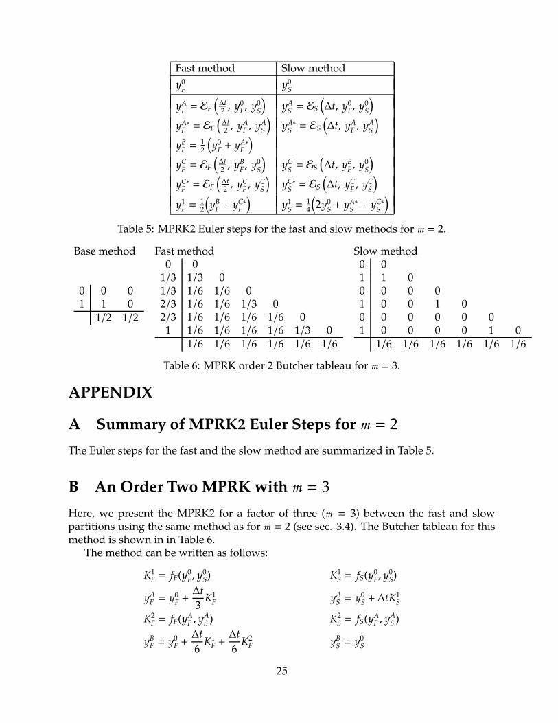
Table 5: MPRK2 Euler steps for the fast and slow methods for m = 2.

Base method Fast method Slow method

0 0 01 1 0

1/2 1/2

0 01/3 1/3 01/3 1/6 1/6 02/3 1/6 1/6 1/3 02/3 1/6 1/6 1/6 1/6 01 1/6 1/6 1/6 1/6 1/3 0

1/6 1/6 1/6 1/6 1/6 1/6

0 01 1 00 0 0 01 0 0 1 00 0 0 0 0 01 0 0 0 0 1 0

1/6 1/6 1/6 1/6 1/6 1/6

Table 6: MPRK order 2 Butcher tableau for m = 3.

APPENDIX

A Summary of MPRK2 Euler Steps for m = 2

The Euler steps for the fast and the slow method are summarized in Table 5.

B An Order Two MPRK with m = 3

Here, we present the MPRK2 for a factor of three (m = 3) between the fast and slowpartitions using the same method as for m = 2 (see sec. 3.4). The Butcher tableau for thismethod is shown in in Table 6.

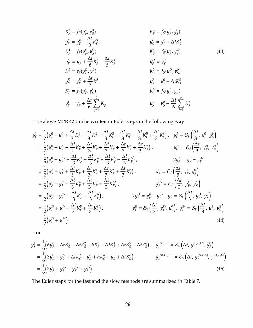
The method can be written as follows:

K1F = fF(y0

F, y0S) K1

S = fS(y0F, y

0S)

yAF = y0

F +∆t

3K1

F yAS = y0

S + ∆tK1S

K2F = fF(yA

F , yAS ) K2

S = fS(yAF , y

AS )

yBF = y0

F +∆t

6K1

F +∆t

6K2

F yBS = y0

S

25

K3F = fF(yB

F , y0S) K3

S = fS(yBF , y

0S)

yCF = yB

F +∆t

3K3

F yCS = y0

S + ∆tK3S

K4F = fF(yC

F , yCS ) K4

S = fS(yCF , y

CS ) (43)

yDF = yB

F +∆t

6K3

F +∆t

6K4

F yDS = y0

S

K5F = fF(yD

F , y0S) K5

S = fS(yDF , y

0S)

yEF = yD

F +∆t

3K5

F yES = y0

S + ∆tK5S

K6F = fF(yE

F , yES) K6

S = fS(yEF , y

ES)

y1F = y0

F +∆t

6

6∑

j=1

Kj

Fy1

S = y0S +∆t

6

6∑

j=1

Kj

S

The above MPRK2 can be written in Euler steps in the following way:

y1F =

1

2

(y0

F + y0F +∆t

3K1

F +∆t

3K2

F +∆t

3K3

F +∆t

3K4

F +∆t

3K5

F +∆t

3K6

F

), yA

F = EF

(∆t

3, y0

F, y0S

)

=1

2

(y0

F + yAF +∆t

2K2

F +∆t

3K3

F +∆t

3K4

F +∆t

3K5

F +∆t

3K6

F

), yA∗

F = EF

(∆t

3, yA

F , yAS

)

=1

2

(y0

F + yA∗F +∆t

3K3

F +∆t

3K4

F +∆t

3K5

F +∆t

3K6

F

), 2yB

F = y0F + yA∗

F

=1

2

(yB

F + yBF +∆t

3K3

F +∆t

3K4

F +∆t

3K5

F +∆t

3K6

F

), yC

F = EF

(∆t

3, yB

F , y0S

)

=1

2

(yB

F + yCF +∆t

3K4

F +∆t

3K5

F +∆t

3K6

F

), yC∗

F = EF

(∆t

3, yC

F , yCS

)

=1

2

(yB

F + yC∗F +∆t

3K5

F +∆t

3K6

F

), 2yD

F = yBF + yC∗

F , yEF = EF

(∆t

3, yD

F , y0S

)

=1

2

(yD

F + yDF +∆t

3K5

F +∆t

3K6

F

), yE

F = EF

(∆t

3, yD

F , y0S

), yE∗

F = EF

(∆t

3, yE

F , yES

)

=1

2

(yD

F + yE∗F

), (44)

and

y1S =

1

6

(6y0

S + ∆tK1S + ∆tK2

S + hK3S + ∆tK4

S + ∆tK5S + ∆tK6

S

), yA,C,E

S= ES

(∆t, y0,B,D

F, y0

S

)

=1

6

(3y0

S + yAS + ∆tK2

S + yCS + hK4

S + yES + ∆tK6

S

), yA∗,C∗,E∗

S= ES

(∆t, yA,C,E

F, yA,C,E

S

)

=1

6

(3y0

S + yA∗S + yC∗

S + yE∗S

). (45)

The Euler steps for the fast and the slow methods are summarized in Table 7.

26

Fast method Slow method

y0F

y0S

yAF = EF

(∆t3, y0

F, y0

S

)yA

S= ES

(∆t, y0

F, y0

S

)

yA∗F= EF

(∆t3, yA

F, yA

S

)yA∗

S= ES

(∆t, yA

F, yA

S

)

yBF= 1

2

(y0

F+ yA∗

F

)

yCF= EF

(∆t3, yB

F, y0S

)yC

S= ES

(∆t, yB

F , y0S

)

yC∗F= EF

(∆t3, yC

F, yC

S

)yC∗

S= ES

(∆t, yC

F, yC

S

)

yDF =

12

(yB

F + yC∗F

)

yEF= EF

(∆t3, yD

F, y0

S

)yE

S= ES

(∆t, yD

F, y0

S

)

yE∗F = EF

(∆t3, yE

F, yES

)yE∗

S= ES

(∆t, yE

F, yES

)

y1F =

12

(yD

F + yC∗F

)y1

S= 1

6

(3y0

S+ yA∗

S+ yC∗

S+ yE∗

S

)

Table 7: MPRK2 Euler steps for the fast and slow methods for m = 3.

27

References

J.F. Andrus. Numerical solution for ordinary differential equations separated into subsys-tems. SIAM Journal of Numerical Analysis, 16(4):605–611, 1979.

J.F. Andrus. Stability of a multirate method for numerical integration of ODEs. Journal ofComputational and Applied Mathematics, 25:3–14, 1993.

A. Bartel and M. Günther. A multirate W-method for electrical networks in state-spaceformulation. Journal of Computational Applied Mathematics, 147(2):411–425, 2002. ISSN0377-0427.

P.J.F. Berkvens, M.A. Botchev, W.M. Lioen, and J.G. Verwer. A zooming technique for windtransport of air pollution. Technical report, Centrum voor Wiskundeen Informatica,1999.

J.P. Boris and D.L. Book. Flux-corrected transport I. SHASTA, a fluid transport algorithmthat works. Journal of Computational Physics, 135(2):172–186, 1997.

S. Chakravarthy and S. Osher. Numerical experiments with the Osher upwind schemefor the Euler equations. AIAA Journal, 21:241–1248, 1983.

S. Chakravarthy and S. Osher. Computing with high-resolution upwind schemes forhyperbolic equations. Lectures in applied mathematics, 22:57–86, 1985.

C. Dawson and R. Kirby. High resolution schemes for conservation laws with locallyvarying time steps. SIAM Journal on Scientific Computing, 22(6):2256–2281, 2001.

B. Engquist and R. Tsai. Heterogeneous multiscale methods for stiff ordinary differentialequations. Mathematics of Computation, 74:1707–1742, 2005.

C. Engstler and C. Lubich. Multirate extrapolation methods for differential equations withdifferent time scales. Computing, 58(2):173–185, 1997. ISSN 0010-485X.

C.W. Gear and D.R. Wells. Multirate linear multistep methods. BIT, 24:484–502, 1984.

S.K. Godunov. A finite difference method for the numerical computation of discontinuoussolutions of the equations of fluid dynamics. Mathematicheskii Sborni, 47:271–290, 1959.

J.B. Goodman, R. LeVeque, and J. Randall. On the accuracy of stable schemes for 2D scalarconservation laws. Mathematics of Computation, 45:15–21, 1985.

S. Gottlieb, C.-W. Shu, and E. Tadmor. Strong stability-preserving high-order time dis-cretization methods. SIAM Review, 43(1):89–112, 2001.

M. Günther and M. Hoschek. ROW methods adapted to electric circuit simulation pack-ages. In ICCAM ’96: Proceedings of the seventh international congress on Computational andapplied mathematics, pages 159–170. Elsevier Science Publishers B. V., 1997.

28

M. Günther, A. Kvaerno, and P. Rentrop. Multirate partitioned Runge-Kutta methods.BIT, 38(2):101–104, 1998.

M. Günther and P. Rentrop. Multirate ROW-methods and latency of electric circuits.Applied Numerical Mathematics, 1993.

E. Hairer. Order conditions for numerical methods for partitioned ordinary differentialequations. Numerische Mathematik, 36(4):431 – 445, 1981.

E. Hairer, S.P. Norsett, and G. Wanner. Solving Ordinary Differential Equations I: NonstiffProblems, chapter II.1. Springer, 1993a.

E. Hairer, S.P. Norsett, and G. Wanner. Solving Ordinary Differential Equations I: NonstiffProblems, chapter II.15. Springer, 1993b.

A. Harten. High resolution schemes for hyperbolic conservation laws. Journal of Compu-tational Physics, 135(2):260–278, 1997. ISSN 0021-9991.

W. Hundsdorfer, B. Koren, and M. van Loon. A positive finite-difference advection scheme.Journal of Computational Physics, 117(1):35–46, 1995.

W. Hundsdorfer, S.J. Ruuth, and R.J. Spiteri. Monotonicity-preserving linear multistepmethods. SIAM Journal on Numerical Analysis, 41(2):605–623, 2003.

T. Kato and T. Kataoka. Circuit analysis by a new multirate method. Electrical Engineeringin Japan, 126(4):55–62, 1999.

R. Kirby. On the convergence of high resolution methods with multiple time scales forhyperbolic conservation laws. Mathematics of Computation, 72(243):1239–1250, 2002.

A. Kværnø. Stability of multirate Runge-Kutta schemes. International Journal of DifferentialEquations and Applications, 1(1):97–105, 2000.

A. Kværnø and P. Rentrop. Low order multirate Runge-Kutta methods in electric circuitsimulation, 1999.

A. Logg. Multi-Adaptive Galerkin Methods for ODEs I. SIAM Journal on Scientific Com-puting, 24(6):1879–1902, 2003a.

A. Logg. Multi-Adaptive Galerkin Methods for ODEs II: Implementation and Applica-tions. SIAM Journal on Scientific Computing, 25(4):1119–1141, 2003b.

A. Logg. Multi-Adaptive Galerkin Methods for ODEs III: Existence and Stability. ChalmersFinite Element Center Preprint Series, (2004-04), 2004.

A. Logg. Multi-Adaptive Galerkin Methods for ODEs III: Apriory Estimates. SIAM Journalof Numerical Analysis, 43(6):2624–2646, 2006.

S. Osher and S. Chakravarthy. High resolution schemes and the entropy condition. SIAMJournal on Numerical Analysis, 21(5):955–984, 1984.

29

S. Osher and S. Chakravarthy. Very high order accurate TVD schemes. Oscillation Theory,Computation, and Methods of Compensated Compactness, IMA Vol. Math. Appl., 2:229–274,1986.

J.R. Rice. Split Runge-Kutta methods for simultaneous equations. Journal of Research of theNational Institute of Standards and Technology, 60(B), 1960.

P.L. Roe. Approximate Riemann solvers, parameter vectors and difference schemes. Journalof Computational Physics, 43:357–372, 1981.

J. Sand and K. Burrage. A jacobi waveform relaxation method for ODEs. SIAM Journal onScientific Computing, 20(2):534–552, 1998. ISSN 1064-8275.

C-W. Shu and S. Osher. Efficient implementation of essentially non-oscillatory shock-capturing schemes. Journal of Computational Physics, 77(2):439–471, 1988. ISSN 0021-9991.

C.-W. Shu and S. Osher. Efficient implementation of essentially non-oscillatory shock-capturing schemes,II. Journal of Computational Physics, 83(1):32–78, 1989. ISSN 0021-9991.

R.J. Spiteri and S.J. Ruuth. A new class of optimal high-order strong-stability-preservingtime discretization methods. SIAM Journal on Numerical Analysis, 40(2):469–491, 2002.

P.K. Sweby. High resolution schemes using flux limiters for hyperbolic conservation laws.SIAM Journal on Numerical Analysis, 21(5):995–1011, 1984.

H.-Z. Tang and G. Warnecke. A class of high resolution schemes for hyperbolic conser-vation laws and convect ion-diffusion equations with varying time and space grids.submitted, 2003.

C.B. Vreugdenhil and B. Koren, editors. Numerical Methods for Advection–Diffusion Problems,volume 45. Vieweg, 1993.

S.T. Zalesak. Fully multidimensional flux corrected transport algorithms for fluids. Journalof Computational Physics, 31:335–362, 1979.

30