Multiresolution Elastic Matching

Lukas Brausch

University of Saarland

Abstract

This summary provides a general overview of the work Multiresolution Elastic Matching [1] written by RuzenaBajcsy and Stanislav Kovacic.

1. Introduction

This section provides a general introduction of thetopics presented in [1] and provides some additionalbackground which is important in order to under-stand the paper. In section 2 the general matchingprocess is introduced and discussed. Section 3 pro-vides more information about the implementationand its details. In section 4 several experiments arepresented to illustrate some results of the presentedpaper. This summary ends with a conclusion pre-sented in section 5.

1.1. Goals

The general idea behind the work presented in [1]is to develop a mechanism to match "an explicit 3-dimensional pictorial model to locally variant data".In other words, two existing representations (onemodel representation and one input representation)are put into correspondence. To achieve this goal,rigid transforms are used to account for global mis-alignments, while elastic deformations are appliedfor local shape differences. A coarse-to-fine strategy(called multiresolution elastic matching) is the heart ofthe presented paper and leads to more efficient com-putations and improved convergence of the matchingprocess in general.

2. The Matching Process

In the presented paper two virtual objects are given:One reference object and one made out of an elasticmaterial. To mimic manual registration, larger dis-parities are corrected in a first step. The second stepconsists of making improvements concerning smallerdisparities. This second step is then repeated until a"satisfactory" match is achieved. The input is givenby brain scans gained from computed tomography(CT). The virtual model is a voxel representation ofan anatomical human brain atlas.

2.1. What needs to be defined?

In general, the presented algorithm aims to find amapping T from a given model M (i.e. the brain atlas)to a pattern P (i.e. the input CT brain scans) usinga similarity measure S. The similarity measure (orsimilarity function) will be discussed in more detail in2.3.3. The following questions have to be answered tohelp the algorithm produce satisfactory results:

• What should be matched ? (i.e. which featuresshould be used in matching?)

• Which constraints should be considered?

• How should be matched? (i.e. which matchingprocess for achieving a consistent match shouldbe applied?)

• How should the match be evaluated? (i.e. howshould the similarity measure be defined?)

2.2. Global Matching

As discussed in 2.3, the elastic matching algorithm isa good choice for smaller changes but it fails if globalmisalignment is too large. To account for larger globalmisalignments global matching is applied first. Thisalgorithm tries to eliminate the effects of the followingthree mayor types of misalignment:

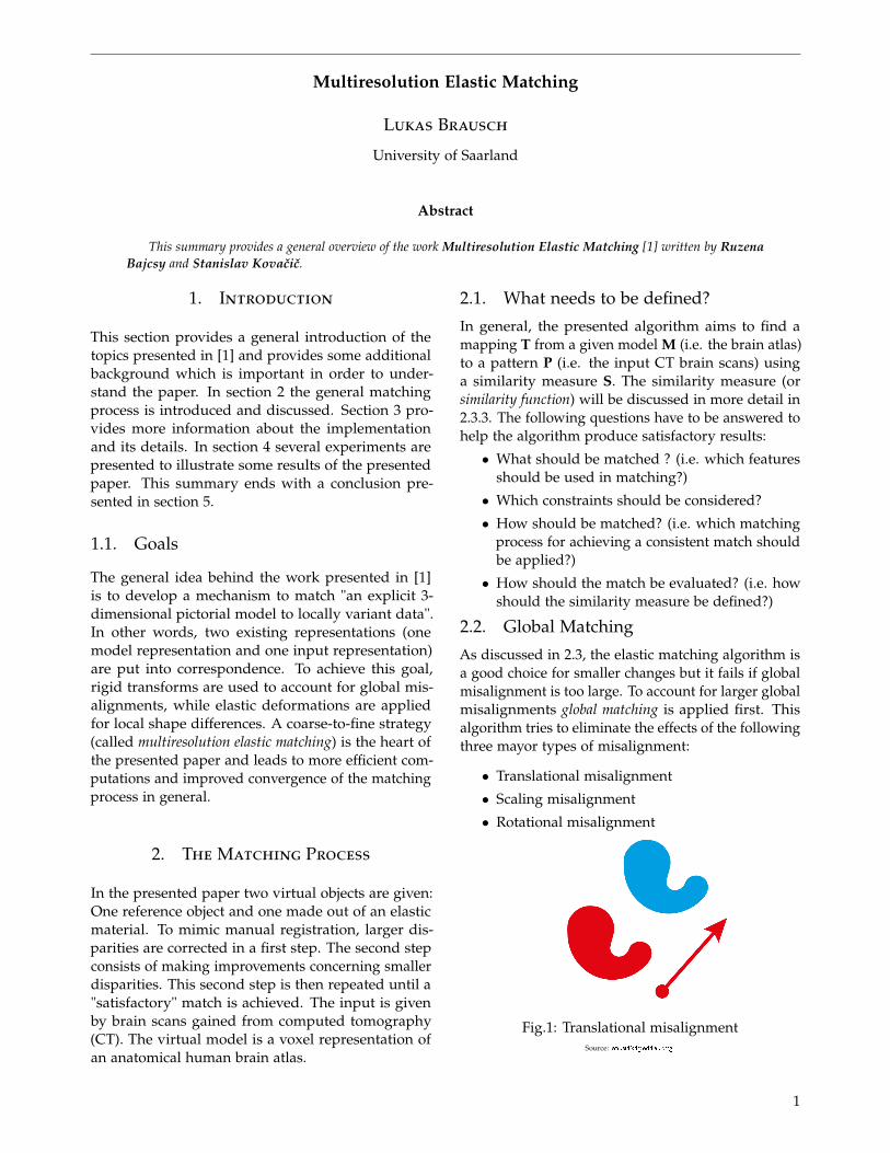
• Translational misalignment

• Scaling misalignment

• Rotational misalignment

Fig.1: Translational misalignmentSource: en.wikipedia.org

1

Fig.2: Scaling misalignmentSource: tutorvista.com

Fig.3: Rotational misalignmentSource: en.wikipedia.org

As seen in Fig.1, translational misalignment depictsthe case in which the objects are (far) away from eachother. In Fig.2 it can be seen that scaling misalignmentmeans that one object is bigger than the other, whileFig.3 shows that rotational misalignment describesthe case in which one object is rotated in a differentdirection than the other.In order to eliminate these misalignments theglobal matching algorithm proceeds in the follow-ing way: Firstly, each object is approximated by"an ellipsoid-like scatter of particles uniformly dis-tributed in space". Translational misalignment isthen eliminated by aligning the centers of massesof both objects. In order to eliminate rotationaland scaling misalignments, the method of principalaxes [2] [3] is used. The covariance matrix is com-puted for each object and an attempt is made toequalize the matrices through rotation and scaling.

Fig.4: Eigenvectors of a covariance matrixSource: http://www.visiondummy.com/2014/04/geometric-interpretation-covariance-matrix/

Fig.4 gives an intuition how the corresponding eigen-vectors and eigenvalues of two different covariancematrices behave. The left image shows the orientationof the point cloud for matrix 1, while the right imagedepicts the orientation for matrix 2.(

5 00 1

)(1)

(1 00 5

)(2)

2.3. Elastic Matching

The basic approach for eliminating small local dispar-ities by using elastic deformations goes back to theDoctoral dissertation of Broit [4]. In it an algorithmis described, which deforms an object until an equi-librium between external forces and resisting internalforces is achieved. This algorithm is based on a partialdifferential equation, which has been developed bythe french scientist Navier in 1822 [5]. This partialdifferential equations reads as follows:

µ4ui + (λ + µ)∂θ

∂xi+ Fi = 0 (i = 1, 2, 3) (3)

u = (u1, u2, u3)T = stands for the sought displace-

ments and θ = ∂u1∂x1

+ ∂u2∂x2

+ ∂u3∂x3

is the cubical dila-tion. The cubical dilation is defined as the quotientof change in volume over the size of the original vol-ume and thus hints at the change in volume due todeformation forces. The parameter x = (x1, x2, x3)

T

describes the coordinate system before any deforma-tion has taken place, while F = (F1, F2, F3)

T standsfor the external forces distributed in the body. Theconstants µ and λ define elastic properties of the body.These elastic properties are an integral part of the de-scription of the corresponding material of each objectand are described in further detail below.

2.3.1 Elastic Properties

As described above, the choice of the elastic proper-ties constants is crucial for a proper modelling of eachobjects material. The authors of this paper decide toset the parameter λ to zero in order to be left withonly one elastic constant. This single constant µ isthen responsible for modelling the material. Experi-ments indicate that a large value of µ leads to morerigid materials (which might, for example, resemblerubber), while a smaller value of µ leads to a solution,which is mostly controlled by external forces. Onedisadvantage of choosing a very small value for µ isthe fact that in this case noise becomes more visibleand false matches occur more frequently. Thus, theauthors hint at deforming the object step by step asthis "should be safer".

2

2.3.2 External forces

An important part of the elastic matching model iswhere and how the external forces are applied toobtain a consistent deformation as they are used toguide the solution locally and globally. The externalforces can be obtained by:

• information from input data

• information from interactive input

• information from a knowledge base

• other processes...

The major task of the external forces is to bring sim-ilar regions in both objects into correspondence. Toachieve this, a similarity measure (as described in2.3.3) between a certain position x = (x1, x2, x3)

T

in the first object and another position x + u =x + (u1, u2, u3)

T in the second object is defined. Notethat the second position already includes a displace-ment u.

2.3.3 Similarity measure

The similarity measure or similarity function at positionx is denoted by S(u). The best local match is expectedfor a displacement vector u which maximizes S(u).If a maximum of S(u) exists, it is also possible to in-crease the similarity by applying a force proportionalto the gradient vector of S(u).If it is assumed that S(u) has continuous secondderivatives, it can be approximated by the followingTaylor series:

S(u + δu) = S(u) + δuT g(u) +12

δuT H(u)δu (4)

As long as only small deformations are taken intoaccount, a quadratic approximation of S(u) can beused:

S(u) =12

uT Au + bTu + c (5)

If this is substituted into the partial differential equa-tion 3 mentioned above, one can get a description forthe applied external forces:

F(u) = g(u) = Au + b (6)

The full notation of this equation reads as follows:

Fi = 2ai1u1 + 2ai2u2 + 2ai3u3 + bi (i = 1, 2, 3) (7)

Those forces are applied in regions in which S(u) hasa maximum. Other regions are not used for matchingas they lack reliable matching information.

2.3.4 Multiresolution Elastic Matching

As already mentioned above, a multi-resolutionstrategy is applied for elastic matching. Thisstrategy has been inspired by multigrid techniquesused in numerical mathematics [6], computa-tional vision [7] [8] and multiresolution pictureprocessing [9]. The idea is similar to imagepyramids for which Fig.5 shows an example.

Fig.5: Sample image pyramidSource: http://vis.berkeley.edu

The basic idea behind such an image pyramid(according to [10]) is to create a series of imageswhich are weighted and scaled down. Whenthis technique is used multiple times, it createsa stack of successively smaller images, with eachpixel containing a local average that correspondsto a pixel neighbourhood on a lower level ofthe pyramid. Fig.6 shows the scheme which hasbeen deployed for the algorithm mentioned in [1].

Fig.6: A multiresolution deformation schemeSource: [1]

3

The image caption of Fig.6 in the original paper readsas follows: "A multiresolution deformation scheme.Features obtained from the resolution pyramid for themodel M and the data D are entered into [the] elasticmatcher. Matching starts on a coarse resolution level.The interpolated solution from coarser level is enteredas the first approximation to the next finer level. Thefinest level solution is used to incrementally deformthe model until a satisfactory match is achieved."

3. Implementation

After discussing the general ideas of the presentedpaper, this section gives some more details about theimplementation. The general steps of the matchingalgorithm are:

1. Preprocessing of the input CT brain scans

2. Preparing the brain atlas for matching

3. Matching the brain atlas with given CT brainscans

4. Overlaying the brain atlas with CT brain scansafter matching

In the following the results of these steps are to bediscussed.

3.1. Preprocessing

Real CT scans of normal patients were used for thefollowing experiments. It was necessary to processthese scans first to obtain usable data.

Preprocessing of the input CT brain scans in-cludes optional low-pass filtering, resampling of theslices, interpolating by linear interpolation to getcubically shaped voxels, selecting an 8-bit grey valuewindow in the original 12-bit range, removing theskull to isolate the brain in CT scans and also theoptional removal of large calcifications (white spots)if present. Fig.7 shows the result of removing theskull in order to isolate the brain.

Fig.7: CT scan before (left) and after (right) isolatingthe brain

Source: [1]

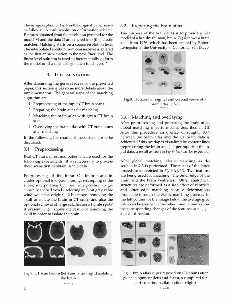
3.2. Preparing the brain atlas

The purpose of the brain atlas is to provide a 3-Dmodel of a healthy (human) brain. Fig.8 shows a brainatlas from 1976, which has been created by RobertLivingston at the University of California, San Diego.

Fig.8: Horizontal, sagittal and coronal views of abrain atlas (1976)

Source: [1]

3.3. Matching and overlayingAfter preprocessing and preparing the brain atlas,global matching is performed as described in 2.2.After this procedure an overlap of roughly 80%between the brain atlas and the CT brain data isachieved. If this overlap is visualized by contour lines(representing the brain atlas) superimposing the in-put data, a result as seen in Fig.9 (left) can be expected.

After global matching, elastic matching as de-scribed in 2.3 is performed. The result of the latterprocedure is depicted in Fig.9 (right). Two featuresare being used for matching: The outer edge of thebrain and the brain ventricles. Other anatomicalstructures are deformed as a side-effect of ventricleand outer edge matching because deformationspropagate through the elastic matching process. Inthe left column of the image below the average greyvalue can be seen while the other three columns showthe corresponding changes of the features in x−, y−and z− direction.

Fig.9: Brain atlas superimposed on CT brains afterglobal alignment (left) and features computed for

particular brain atlas sections (right)Source: [1]4

4. Experiments

The following experiments are meant to give thereader some more intuition about the discussed ideasand algorithms.

4.1. Elastic constantsAs already seen in 2.3.1 elastic constants play a bigrole in determining which properties a modelled ma-terial has. Hence, they are also very important forthe elastic matching process in general as Fig.10 (left)shows vividly. The left column depicts the matchingstate after performing global alignment. The threecolumns to the right show matching results for anelastic constant value of 8, 4 and 1 respectively.

Fig.10: Matching between two brain atlases usingdifferent elastic constants (left) and deformation at

successive stages (right)Source: [1]

To show that not only the elastic constants but alsothe number of iterations of the elastic matching pro-cess influences the final result, Fig.10 (right) illustratesthe result of the matching process with a fixed elasticconstant of value 2. The first column shows the resultafter global alignment while the next three columnsto the right depict the result after successive defor-mations. It can be easily seen that better results areachieved with more iterations.

Fig.11: Two brain atlases superimposed after globalalignment (left) and elastic matching (right)

Source: [1]

In Fig.11 it can be seen that it is also possible to matchtwo brain atlases with each other. The left pictureillustrates the matching result after global alignmentand the right picture the result after elastic matching.Fig.12 (left) hints at the possibility of matching thebrain atlas to different brains. In this example eachrow shows a different CT brain. Lastly, Fig.12 (right)presents all matching ideas of this paper by show-ing one brain atlas slice after global matching, elasticmatching and scaling it back to the original CT pixelsize.

Fig.12: (Elastic) matching the brain atlas to threedifferent brains (left) and example including all

presented matching steps (right)Source: [1]

5. Conclusion

The main contribution of the presented paper is thedevelopment of a general method for matching 3-Dpatterns with a 3-D model. To achieve this goal, rigidtransforms are used for global misalignment and elas-tic deformations are used for local shape differences.A coarse-to-fine strategy approach is applied whichleads to more efficient computations and improvedconvergence of the matching process in general. Thematching algorithm is performed in 3-D.

References

[1] Bajcsy R and Kovacic S. Multiresolution elasticmatching. Computer Vision, Graphics, and ImageProcessing 46, 1 - 2 1, 1989.

[2] Horn B. K. P. Robot vision. Robot Vision, MIT,Cambridge, MA, 1986.

[3] Rosenfeld A and Kak A. Digital picture process-ing. Academic Press, New York, 1982.

[4] Broit C. Optimal registration of deformed im-ages. Doctoral dissertation, University of Pennsylva-nia, Philadelphia, 1981.

[5] Sokolnikoff I, S. Mathematical theory of elasticity.McGraw-Hill, New York, 1956.

[6] Brandt A. Multi-level adaptive techniques forboundary-value problems. Math. Comput., 31, No.138, 1977, 333-390, 1977.

[7] Terzopoulos D. Multilevel computational pro-cesses for visual surface reconstruction. Comput.Vision Graphics Image Process., 24, No. 1, 1983, 52-96., 1983.

[8] Terzopoulos D. Multiresolution computation ofvisible-surface representations. Doctoral disserta-tion, MIT, January 1984, 1984.

[9] Butt P and Adelson T. The laplacian pyramid asa compact image code. IEEE Trans. Commun. 31,No. 4, 1983, 532-540, 1983.

[10] Gaussian pyramid, wikipedia article. https:

//en.wikipedia.org/wiki/Gaussian_pyramid.

5