1

Multiscale Combinatorial Groupingfor Image Segmentation andObject Proposal Generation

Jordi Pont-Tuset*, Pablo Arbelaez*, Jonathan T. Barron, Member, IEEE,Ferran Marques, Senior Member, IEEE, Jitendra Malik, Fellow, IEEE

Abstract—We propose a unified approach for bottom-up hierarchical image segmentation and object proposal generation forrecognition, called Multiscale Combinatorial Grouping (MCG). For this purpose, we first develop a fast normalized cuts algorithm.We then propose a high-performance hierarchical segmenter that makes effective use of multiscale information. Finally, we propose agrouping strategy that combines our multiscale regions into highly-accurate object proposals by exploring efficiently their combinatorialspace. We also present Single-scale Combinatorial Grouping (SCG), a faster version of MCG that produces competitive proposals inunder five second per image. We conduct an extensive and comprehensive empirical validation on the BSDS500, SegVOC12, SBD,and COCO datasets, showing that MCG produces state-of-the-art contours, hierarchical regions, and object proposals.

Index Terms—Image segmentation, object proposals, normalized cuts.

F

1 INTRODUCTION

TWO paradigms have shaped the field of object recog-nition in the last decade. The first one, popularized

by the Viola-Jones face detection algorithm [1], formu-lates object localization as window classification. The ba-sic scanning-window architecture, relying on histogramsof gradients and linear support vector machines, wasintroduced by Dalal and Triggs [2] in the context ofpedestrian detection and is still at the core of seminalobject detectors on the PASCAL challenge such as De-formable Part Models [3].

The second paradigm relies on perceptual grouping toprovide a limited number of high-quality and category-independent object proposals, which can then be de-scribed with richer representations and used as input tomore sophisticated learning methods. Examples in thisfamily are [4], [5]. Recently, this approach has dominatedthe PASCAL segmentation challenge [6], [7], [8], [9], im-proved object detection [10], fine-grained categorization[11] and proven competitive in large-scale classification[12].

Since the power of this second paradigm is criticallydependent on the accuracy and the number of objectproposals, an increasing body of research has delved

• J. Pont-Tuset and F. Marques are with the Department of Signal Theoryand Communications, Universitat Politecnica de Catalunya, BarcelonaTech(UPC), Spain. E-mail: {jordi.pont,ferran.marques}@upc.edu

• P. Arbelaez is with the Department of Biomedical Engineering, Universi-dad de los Andes, Colombia. E-mail: pa.arbelaez@uniandes.edu.co

• J. T. Barron, and J. Malik are with the Department of ElectricalEngineering and Computer Science, University of California at Berkeley,Berkeley, CA 94720. E-mail: {barron,malik}@eecs.berkeley.edu

* The first two authors contributed equally

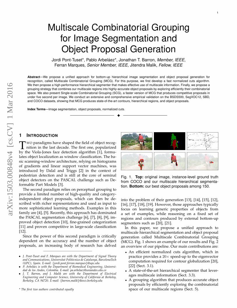
Fig. 1. Top: original image, instance-level ground truthfrom COCO and our multiscale hierarchical segmenta-tion. Bottom: our best object proposals among 150.

into the problem of their generation [13], [14], [15], [12],[16], [17], [18], [19]. However, those approaches typicallyfocus on learning generic properties of objects froma set of examples, while reasoning on a fixed set ofregions and contours produced by external bottom-upsegmenters such as [20], [21].

In this paper, we propose a unified approach tomultiscale hierarchical segmentation and object proposalgeneration called Multiscale Combinatorial Grouping(MCG). Fig. 1 shows an example of our results and Fig. 2an overview of our pipeline. Our main contributions are:

• An efficient normalized cuts algorithm, which inpractice provides a 20× speed-up to the eigenvectorcomputation required for contour globalization [20],[22] (Sect. 3.1).

• A state-of-the-art hierarchical segmenter that lever-ages multiscale information (Sect. 3.3).

• A grouping algorithm that produces accurate objectproposals by efficiently exploring the combinatorialspace of our multiscale regions (Sect. 5).

arX

iv:1

503.

0084

8v4

[cs

.CV

] 1

Mar

201

6

2

F ixed-ScaleSegmentation

R escaling &A lignment

C ombination

Re

solu

tio

n

C ombinatorialGrouping

I mage P yramid Segmentati on P yramid Al i gned H ierarchies Object Proposals Multiscale Hierarchy

Fig. 2. Multiscale Combinatorial Grouping. Starting from a multiresolution image pyramid, we perform hierarchicalsegmentation at each scale independently. We align these multiple hierarchies and combine them into a singlemultiscale segmentation hierarchy. Our grouping component then produces a ranked list of object proposals byefficiently exploring the combinatorial space of these regions.

We conduct a comprehensive and large-scale empiricalvalidation. On the BSDS500 (Sect. 4) we report significantprogress in contour detection and hierarchical segmen-tation. On the VOC2012, SBD, and COCO segmentationdatasets (Sect. 6), our proposals obtain overall state-of-the-art accuracy both as segmented proposals and asbounding boxes. MCG is efficient, its good generaliza-tion power makes it parameter free in practice, and itprovides a ranked set of proposals that are competitivein all regimes of number of proposals.

2 RELATED WORKFor space reasons, we focus our review on recent normal-ized cut algorithms and object proposals for recognition.

Fast normalized cuts: The efficient computation ofnormalized-cuts eigenvectors has been the subject ofrecent work, as it is often the computational bottleneckin grouping algorithms. Taylor [23] presented a tech-nique for using a simple watershed oversegmentationto reduce the size of the eigenvector problem, sacri-ficing accuracy for speed. We take a similar approachof solving the eigenvector problem in a reduced space,though we use simple image-pyramid operations onthe affinity matrix (instead of a separate segmentationalgorithm) and we see no loss in performance despite a20× speed improvement. Maire and Yu [24] presenteda novel multigrid solver for producing eigenvectors atmultiple scales, which speeds up fine-scale eigenvectorcomputation by leveraging coarse-scale solutions. Ourtechnique also uses the scale-space structure of an image,but instead of solving the problem at multiple scales,we simply reduce the scale of the problem, solve it ata reduced scale, and then upsample the solution whilepreserving the structure of the image. As such, ourtechnique is faster and much simpler, requiring only afew lines of code wrapped around a standard sparseeigensolver.

Object Proposals: Class-independent methods thatgenerate object hypotheses can be divided into thosewhose output is an image window and those that gen-erate segmented proposals.

Among the former, Alexe et al. [16] propose an ob-jectness measure to score randomly-sampled image win-dows based on low-level features computed on thesuperpixels of [21]. Manen et al. [25] propose to use theRandomized Prim’s algorithm, Zitnick et al. [26] groupcontours directly to produce object windows, and Chenget al. [27] generate box proposals at 300 images persecond. In contrast to these approaches, we focus onthe finer-grained task of pixel-accurate object extraction,rather than on window selection. However, by just tak-ing the bounding box around our segmented proposals,our results are also state of the art as window proposals.

Among the methods that produce segmented propos-als, Carreira and Sminchisescu [18] hypothesize a set ofplacements of fore- and background seeds and, for eachconfiguration, solve a constrained parametric min-cut(CPMC) problem to generate a pool of object hypotheses.Endres and Hoiem [19] base their category-independentobject proposals on an iterative generation of a hierarchyof regions, based on the contour detector of [20] andocclusion boundaries of [28]. Kim and Grauman [17]propose to match parts of the shape of exemplar objects,regardless of their class, to detected contours by [20].They infer the presence and shape of a proposal objectby adapting the matched object to the computed super-pixels.

Uijlings et al. [12] present a selective search algorithmbased on segmentation. Starting with the superpixelsof [21] for a variety of color spaces, they produce a set ofsegmentation hierarchies by region merging, which areused to produce a set of object proposals. While we alsotake advantage of different hierarchies to gain diversity,we leverage multiscale information rather than different

3

color spaces.Recently, two works proposed to train a cascade of

classifiers to learn which sets of regions should bemerged to form objects. Ren and Shankhnarovich [29]produce full region hierarchies by iteratively mergingpairs of regions and adapting the classifiers to differentscales. Weiss and Taskar [30] specialize the classifiers alsoto size and class of the annotated instances to produceobject proposals.

Malisiewicz and Efros [4] took one of the first stepstowards combinatorial grouping, by running multiplesegmenters with different parameters and merging upto three adjacent regions. In [8], another step was takenby considering hierarchical segmentations at three differ-ent scales and combining pairs and triplets of adjacentregions from the two coarser scales to produce objectproposals.

The most recent wave of object proposal algorithmsis represented by [13], [14], and [15], which all keep thequality of the seminal proposal works while improvingthe speed considerably. Krahenbuhl and Koltun [13]find object proposal by identifying critical level setsin geodesic distance transforms, based on seeds placedin learnt places in the image. Rantalankila et al. [14]perform a global and local search in the space of setsof superpixels. Humayun et al. [15] reuse a graph toperform many parametric min-cuts over different seedsin order to speed the process up.

A substantial difference between our approach andprevious work is that, instead of relying on pre-computed hierarchies or superpixels, we propose a uni-fied approach that produces and groups high-qualitymultiscale regions. With respect to the combinatorial ap-proaches of [4], [8], our main contribution is to developefficient algorithms to explore a much larger combinato-rial space by taking into account a set of object examples,increasing thus the likelihood of having complete objectsin the pool of proposals. Our approach has thereforethe flexibility to adapt to specific applications and typesof objects, and can produce proposals at any trade-offbetween their number and their accuracy.

3 THE SEGMENTATION ALGORITHM

Consider a segmentation of the image into regions thatpartition its domain S = {Si}i. A segmentation hierarchyis a family of partitions {S∗,S1, ...,SL} such that: (1)S∗ is the finest set of superpixels, (2) SL is the completedomain, and (3) regions from coarse levels are unions ofregions from fine levels. A hierarchy where each level Siis assigned a real-valued index λi can be represented by adendrogram, a region tree where the height of each nodeis its index. Furthermore, it can also be represented as anultrametric contour map (UCM), an image obtained byweighting the boundary of each pair of adjacent regionsin the hierarchy by the index at which they are merged[31], [32]. This representation unifies the problems ofcontour detection and hierarchical image segmentation:

ThresholdMerging-sequencepartitions

λ*

λ1

λ2

λL

Region Tree (dendrogram)

*

#

#

#

SL

S2

S1

S*

Ultrametric Contour Map

Fig. 3. Duality between a UCM and a region tree:Schematic view of the dual representation of a seg-mentation hierarchy as a region dendrogram and as anultrametric contour map.

a threshold at level λi in the UCM produces the segmen-tation Si.

Figure 3 schematizes these concepts. First, the lowerleft corner shows the probability of boundary of a UCM.One of the main properties of a UCM is that when wethreshold the contour strength at a certain value, weobtain a closed boundary map, and thus a partition.Thresholding at different λi, therefore, we obtain theso-called merging-sequence partitions (left column inFigure 3); named after the fact that a step in this sequencecorresponds to merging the set of regions sharing theboundary of strength exactly λi.

For instance, the boundary between the wheels andthe floor has strength λ1, thus thresholding the contourabove λ1 makes the wheels merge with the floor. If werepresent the regions in a partition as nodes of a graph,we can then represent the result of merging them as theirparent in a tree. The result of sweeping all λi valuescan therefore be represented as a region tree, whose rootis the region representing the whole image (right partof Figure 3). Given that each merging is associated witha contour strength, the region tree is in fact a regiondendogram.

As an example, in the gPb-ucm algorithm of [20],brightness, color and texture gradients at three fixed disksizes are first computed. These local contour cues areglobalized using spectral graph-partitioning, resulting inthe gPb contour detector. Hierarchical segmentation isthen performed by iteratively merging adjacent regionsbased on the average gPb strength on their commonboundary. This algorithm produces therefore a tree ofregions at multiple levels of homogeneity in brightness,color and texture, and the boundary strength of its UCMcan be interpreted as a measure of contrast.

Coarse-to-fine is a powerful processing strategy incomputer vision. We exploit it in two different waysto develop an efficient, scalable and high-performancesegmentation algorithm: (1) To speed-up spectral graphpartitioning and (2) To create aligned segmentation hi-erarchies.

4

3.1 Fast Downsampled Eigenvector Computation

The normalized cuts criterion is a key globalizationmechanism of recent high-performance contour detec-tors such as [20], [22]. Although powerful, such spectralgraph partitioning has a significant computational costand memory footprint that limit its scalability. In thissection, we present an efficient normalized cuts approx-imation which in practice preserves full performance forcontour detection, while having low memory require-ments and providing a 20× speed-up.

Given a symmetric affinity matrix A, we would liketo compute the k smallest eigenvectors of the Laplacianof A. Directly computing such eigenvectors can be verycostly even with sophisticated solvers, due to the largesize of A. We therefore present a technique for efficientlyapproximating the eigenvector computation by takingadvantage of the multiscale nature of our problem: Amodels affinities between pixels in an image, and imagesnaturally lend themselves to multiscale or pyramid-likerepresentations and algorithms.

Our algorithm is inspired by two observations: 1) ifA is bistochastic (the rows and columns of A sum to 1)then the eigenvectors of the Laplacian A are equal tothe eigenvectors of the Laplacian of A2, and 2) becauseof the scale-similar nature of images, the eigenvectorsof a “downsampled” version of A in which every otherpixel has been removed should be similar to the eigen-vectors of A. Let us define pixel decimate (A), whichtakes an affinity matrix A and returns the set of indicesof rows/columns in A corresponding to a decimatedversion of the image from which A was constructed. Thatis, if i = pixel decimate (A), then A [i, i] is a decimatedmatrix in which alternating rows and columns of the im-age have been removed. Computing the eigenvectors ofA [i, i] works poorly, as decimation disconnects pixels inthe affinity matrix, but the eigenvectors of the decimatedsquared affinity matrix A2 [i, i] are similar to those of A,because by squaring the matrix before decimation weintuitively allow each pixel to propagate information toall of its neighbors in the graph, maintaining connec-tions even after decimation. Our algorithm works byefficiently computing A2 [i, i] as A [:, i]

TA [:, i]1 (the naive

approach of first squaring A and then decimating it isprohibitively expensive), computing the eigenvectors ofA2 [i, i], and then “upsampling” those eigenvectors backto the space of the original image by pre-multiplyingby A [:, i]. This squaring-and-decimation procedure canbe applied recursively several times, each applicationimproving efficiency while slightly sacrificing accuracy.

Pseudocode for our algorithm, which we call“DNCuts” (Downsampled Normalized Cuts) is given inAlgorithm 1, where A is our affinity matrix and d isthe number of times that our squaring-and-decimationoperation is applied. Our algorithm repeatedly appliesour joint squaring-and-decimation procedure, computes

1. The Matlab-like notation A [:, i] indicates keeping the columns ofmatrix A whose indices are in the set i.

Algorithm 1 dncuts(A, d, k)

1: A0 ← A2: for s = [1, 2, . . . , d] do3: is ← pixel decimate (As−1)4: Bs ← As−1 [ : , is ]5: Cs ← diag(Bs~1)

−1Bs6: As ← CT

s Bs7: end for8: Xd ← ncuts(Ad, k)9: for s = [d, d− 1, . . . , 1] do

10: Xs−1 ← CsXs

11: end for12: return whiten(X0)

Fig. 4. Example of segmentation projection. In order to“snap” the boundaries of a segmentation R (left) to thoseof a segmentation S (middle), since they do not align, wecompute π(R,S) (right) by assigning to each segment inS its mode among the labels of R.

the smallest k eigenvectors of the final “downsam-pled” matrix Ad by using a standard sparse eigensolverncuts(Ad, k), and repeatedly “upsamples” those eigen-vectors. Because our A is not bistochastic and decimationis not an orthonormal operation, we must do somenormalization throughout the algorithm (line 5) andwhiten the resulting eigenvectors (line 10). We found thatvalues of d = 2 or d = 3 worked well in practice. Largervalues of d yielded little speed improvement (as much ofthe cost is spent downsampling A0) and start negativelyaffecting accuracy. Our technique is similar to Nystrom’smethod for computing the eigenvectors of a subset of A,but our squaring-and-decimation procedure means thatwe do not depend on long-range connections betweenpixels.

3.2 Aligning Segmentation HierarchiesIn order to leverage multi-scale information, our ap-proach combines segmentation hierarchies computedindependently at multiple image resolutions. How-ever, since subsampling an image removes details andsmooths away boundaries, the resulting UCMs are mis-aligned, as illustrated in the second panel of Fig. 2. In thissection, we propose an algorithm to align an arbitrarysegmentation hierarchy to a target segmentation and,in Sect. 5, we show its effectiveness for multi-scalesegmentation.

The basic operation is to “snap” the boundaries of asegmentation R = {Ri}i to a segmentation S = {Sj}j , asillustrated in Fig. 4. For this purpose, we define L(Sj),

5

the new label of a region Sj ∈ S, as the majority label ofits pixels in R:

L(Sj) = argmaxi

|Sj ∩Ri||Sj |

(1)

We call the segmentation defined by this new labeling ofall the regions of S the projection of R onto S and denoteit by π(R,S).

In order to project an UCM onto a target segmentationS , which we denote π(UCM,S), we project in turn eachof the levels of the hierarchy onto S. Note that, sinceall the levels are projected onto the same segmentation,the family of projections is by construction a hierar-chy of segmentations. This procedure is summarized inpseudo-code in Algorithm 2.

Algorithm 2 UCM Rescaling and AlignmentRequire: An UCM with a set of levels [t1, ..., tK ]Require: A target segmentation S∗

1: UCMπ ← 02: for t = [t1, ..., tK ] do3: S ← sampleHierarchy(UCM, t)4: S ← rescaleSegmentation(S,S∗)5: S ← π(S,S∗)6: contours← extractBoundary(S)7: UCMπ ← max(UCMπ, t ∗ contours)8: end for9: return UCMπ

Observe that the routines sampleHierarchy andextractBoundary can be computed efficiently becausethey involve only thresholding operations and connectedcomponents labeling. The complexity is thus dominatedby rescaleSegmentation in Step 4, a nearest neighborinterpolation, and the projection in Step 5, which arecomputed K times.

3.3 Multiscale Hierarchical SegmentationSingle-scale segmentation: We consider as input

the following local contour cues: (1) brightness, color andtexture differences in half-disks of three sizes [33], (2)sparse coding on patches [22], and (3) structured forestcontours [34]. We globalize the contour cues indepen-dently using our fast eigenvector gradients of Sect. 3.1,combine global and local cues linearly, and constructan UCM based on the mean contour strength. We triedlearning weights using gradient ascent on the F-measureon the training set [20], but evaluating the final hierar-chies rather than open contours. We observed that thisobjective favors the quality of contours at the expense ofregions and obtained better overall results by optimizingthe Segmentation Covering metric [20].

Hierarchy Alignment: We construct a multiresolu-tion pyramid with N scales by subsampling / super-sampling the original image and applying our single-scale segmenter. In order to preserve thin structuresand details, we declare as set of possible boundary

locations the finest superpixels in the highest-resolution.Then, applying recursively Algorithm 2, we project eachcoarser UCM onto the next finer scale until aligning itto the highest resolution superpixels.

Multiscale Hierarchy: After alignment, we have afixed set of boundary locations, and N strengths foreach of them, coming from the different scales. Weformulate this problem as binary boundary classificationand train a classifier that combines these N features intoa single probability of boundary estimation. We exper-imented with several learning strategies for combiningUCM strengths: (a) Uniform weights transformed intoprobabilities with Platt’s method. (b) SVMs and logisticregression, with both linear and additive kernels. (c)Random Forests. (d) The same algorithm as for single-scale. We found the results with all learning methodssurprisingly similar, in agreement with the observationreported by [33]. This particular learning problem, withonly a handful of dimensions and millions of data points,is relatively easy and performance is mainly driven byour already high-performing and well calibrated fea-tures. We therefore use the simplest option (a).

4 EXPERIMENTS ON THE BSDS500We conduct extensive experiments on the BSDS500 [35],using the standard evaluation metrics and following thebest practice rules of that dataset. We also report resultswith a recent evaluation metric Fop [36], [37], Precision-Recall for objects and parts, using the publicly-availablecode.

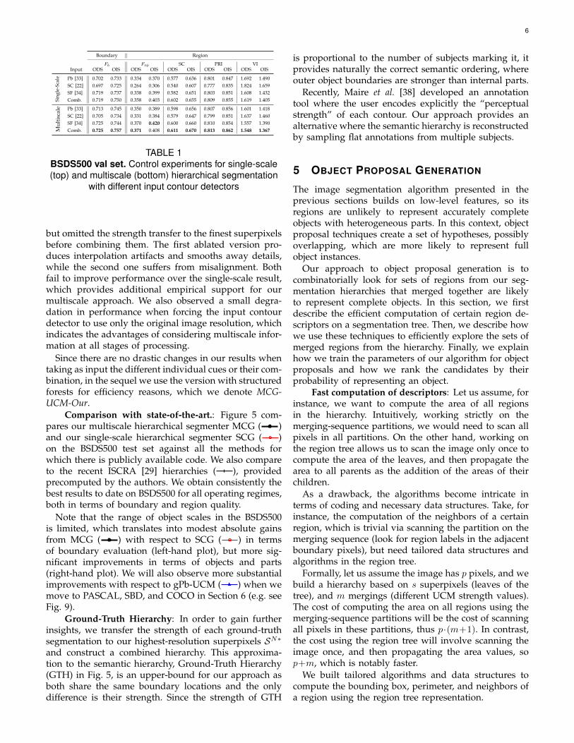
Single-scale Segmentation: Table 1-top shows theperformance of our single-scale segmenter for differenttypes of input contours on the validation set of theBSDS500. We obtain high-quality hierarchies for all thecues considered, showing the generality of our approach.Furthermore, when using them jointly (row ’Comb.’in top panel), our segmenter outperforms the versionswith individual cues, suggesting its ability to leveragediversified inputs. In terms of efficiency, our fast nor-malized cuts algorithm provides an average 20× speed-up over [20], starting from the same local cues, withno significant loss in accuracy and with a low memoryfootprint.

Multiscale Segmentation: Table 1-bottom evaluatesour full approach in the same experimental conditions asthe upper panel. We observe a consistent improvementin performance in all the metrics for all the inputs, whichvalidates our architecture for multiscale segmentation.We experimented with the range of scales and foundN = {0.5, 1, 2} adequate for our purposes. A finersampling or a wider range of scales did not providenoticeable improvements. We tested also two degradedversions of our system (not shown in the table). Forthe first one, we resized contours to the original imageresolution, created UCMs and combined them with thesame method as our final system. For the second one, wetransformed per-scale UCMs to the original resolution,

6

Boundary Region

Fb Fop SC PRI VIInput ODS OIS ODS OIS ODS OIS ODS OIS ODS OIS

Sing

le-S

cale Pb [33] 0.702 0.733 0.334 0.370 0.577 0.636 0.801 0.847 1.692 1.490

SC [22] 0.697 0.725 0.264 0.306 0.540 0.607 0.777 0.835 1.824 1.659SF [34] 0.719 0.737 0.338 0.399 0.582 0.651 0.803 0.851 1.608 1.432Comb. 0.719 0.750 0.358 0.403 0.602 0.655 0.809 0.855 1.619 1.405

Mul

tisc

ale Pb [33] 0.713 0.745 0.350 0.389 0.598 0.656 0.807 0.856 1.601 1.418

SC [22] 0.705 0.734 0.331 0.384 0.579 0.647 0.799 0.851 1.637 1.460SF [34] 0.725 0.744 0.370 0.420 0.600 0.660 0.810 0.854 1.557 1.390Comb. 0.725 0.757 0.371 0.408 0.611 0.670 0.813 0.862 1.548 1.367

TABLE 1BSDS500 val set. Control experiments for single-scale(top) and multiscale (bottom) hierarchical segmentation

with different input contour detectors

but omitted the strength transfer to the finest superpixelsbefore combining them. The first ablated version pro-duces interpolation artifacts and smooths away details,while the second one suffers from misalignment. Bothfail to improve performance over the single-scale result,which provides additional empirical support for ourmultiscale approach. We also observed a small degra-dation in performance when forcing the input contourdetector to use only the original image resolution, whichindicates the advantages of considering multiscale infor-mation at all stages of processing.

Since there are no drastic changes in our results whentaking as input the different individual cues or their com-bination, in the sequel we use the version with structuredforests for efficiency reasons, which we denote MCG-UCM-Our.

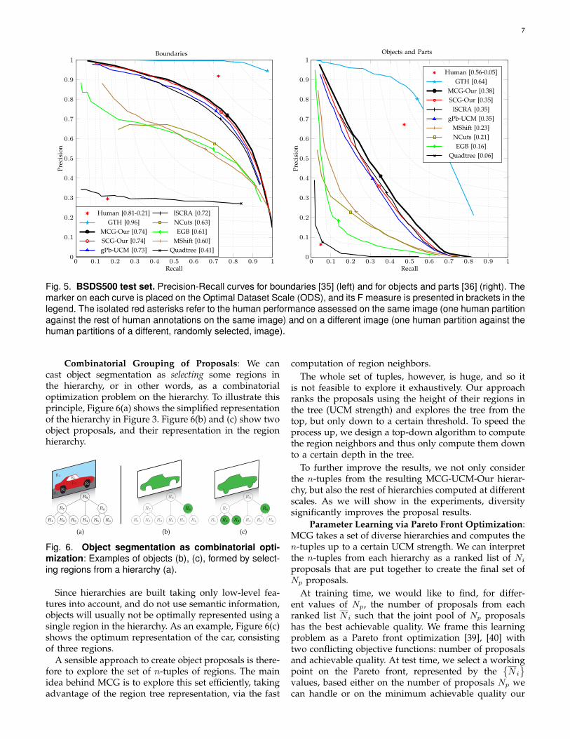
Comparison with state-of-the-art.: Figure 5 com-pares our multiscale hierarchical segmenter MCG ( )and our single-scale hierarchical segmenter SCG ( )on the BSDS500 test set against all the methods forwhich there is publicly available code. We also compareto the recent ISCRA [29] hierarchies ( ), providedprecomputed by the authors. We obtain consistently thebest results to date on BSDS500 for all operating regimes,both in terms of boundary and region quality.

Note that the range of object scales in the BSDS500is limited, which translates into modest absolute gainsfrom MCG ( ) with respect to SCG ( ) in termsof boundary evaluation (left-hand plot), but more sig-nificant improvements in terms of objects and parts(right-hand plot). We will also observe more substantialimprovements with respect to gPb-UCM ( ) when wemove to PASCAL, SBD, and COCO in Section 6 (e.g. seeFig. 9).

Ground-Truth Hierarchy: In order to gain furtherinsights, we transfer the strength of each ground-truthsegmentation to our highest-resolution superpixels SN∗

and construct a combined hierarchy. This approxima-tion to the semantic hierarchy, Ground-Truth Hierarchy(GTH) in Fig. 5, is an upper-bound for our approach asboth share the same boundary locations and the onlydifference is their strength. Since the strength of GTH

is proportional to the number of subjects marking it, itprovides naturally the correct semantic ordering, whereouter object boundaries are stronger than internal parts.

Recently, Maire et al. [38] developed an annotationtool where the user encodes explicitly the “perceptualstrength” of each contour. Our approach provides analternative where the semantic hierarchy is reconstructedby sampling flat annotations from multiple subjects.

5 OBJECT PROPOSAL GENERATION

The image segmentation algorithm presented in theprevious sections builds on low-level features, so itsregions are unlikely to represent accurately completeobjects with heterogeneous parts. In this context, objectproposal techniques create a set of hypotheses, possiblyoverlapping, which are more likely to represent fullobject instances.

Our approach to object proposal generation is tocombinatorially look for sets of regions from our seg-mentation hierarchies that merged together are likelyto represent complete objects. In this section, we firstdescribe the efficient computation of certain region de-scriptors on a segmentation tree. Then, we describe howwe use these techniques to efficiently explore the sets ofmerged regions from the hierarchy. Finally, we explainhow we train the parameters of our algorithm for objectproposals and how we rank the candidates by theirprobability of representing an object.

Fast computation of descriptors: Let us assume, forinstance, we want to compute the area of all regionsin the hierarchy. Intuitively, working strictly on themerging-sequence partitions, we would need to scan allpixels in all partitions. On the other hand, working onthe region tree allows us to scan the image only once tocompute the area of the leaves, and then propagate thearea to all parents as the addition of the areas of theirchildren.

As a drawback, the algorithms become intricate interms of coding and necessary data structures. Take, forinstance, the computation of the neighbors of a certainregion, which is trivial via scanning the partition on themerging sequence (look for region labels in the adjacentboundary pixels), but need tailored data structures andalgorithms in the region tree.

Formally, let us assume the image has p pixels, and webuild a hierarchy based on s superpixels (leaves of thetree), and m mergings (different UCM strength values).The cost of computing the area on all regions using themerging-sequence partitions will be the cost of scanningall pixels in these partitions, thus p·(m+1). In contrast,the cost using the region tree will involve scanning theimage once, and then propagating the area values, sop+m, which is notably faster.

We built tailored algorithms and data structures tocompute the bounding box, perimeter, and neighbors ofa region using the region tree representation.

7

Boundaries

0 0.1 0.2 0.3 0.4 0.5 0.6 0.7 0.8 0.9 10

0.1

0.2

0.3

0.4

0.5

0.6

0.7

0.8

0.9

1

Recall

Prec

isio

n

Human [0.81-0.21] ISCRA [0.72]GTH [0.96] NCuts [0.63]

MCG-Our [0.74] EGB [0.61]SCG-Our [0.74] MShift [0.60]gPb-UCM [0.73] Quadtree [0.41]

Objects and Parts

0 0.1 0.2 0.3 0.4 0.5 0.6 0.7 0.8 0.9 10

0.1

0.2

0.3

0.4

0.5

0.6

0.7

0.8

0.9

1

Recall

Prec

isio

n

Human [0.56-0.05]GTH [0.64]

MCG-Our [0.38]SCG-Our [0.35]

ISCRA [0.35]gPb-UCM [0.35]

MShift [0.23]NCuts [0.21]EGB [0.16]

Quadtree [0.06]

Fig. 5. BSDS500 test set. Precision-Recall curves for boundaries [35] (left) and for objects and parts [36] (right). Themarker on each curve is placed on the Optimal Dataset Scale (ODS), and its F measure is presented in brackets in thelegend. The isolated red asterisks refer to the human performance assessed on the same image (one human partitionagainst the rest of human annotations on the same image) and on a different image (one human partition against thehuman partitions of a different, randomly selected, image).

Combinatorial Grouping of Proposals: We cancast object segmentation as selecting some regions inthe hierarchy, or in other words, as a combinatorialoptimization problem on the hierarchy. To illustrate thisprinciple, Figure 6(a) shows the simplified representationof the hierarchy in Figure 3. Figure 6(b) and (c) show twoobject proposals, and their representation in the regionhierarchy.

R4

R5

R1R2

R3

R6

R9

R7

R1 R2 R3 R4

R8

R5 R6

(a)

R9

R7

R1 R2 R3 R4

R8

R5 R6

(b)

R9

R7

R1 R2 R3 R4

R8

R5 R6

(c)

Fig. 6. Object segmentation as combinatorial opti-mization: Examples of objects (b), (c), formed by select-ing regions from a hierarchy (a).

Since hierarchies are built taking only low-level fea-tures into account, and do not use semantic information,objects will usually not be optimally represented using asingle region in the hierarchy. As an example, Figure 6(c)shows the optimum representation of the car, consistingof three regions.

A sensible approach to create object proposals is there-fore to explore the set of n-tuples of regions. The mainidea behind MCG is to explore this set efficiently, takingadvantage of the region tree representation, via the fast

computation of region neighbors.The whole set of tuples, however, is huge, and so it

is not feasible to explore it exhaustively. Our approachranks the proposals using the height of their regions inthe tree (UCM strength) and explores the tree from thetop, but only down to a certain threshold. To speed theprocess up, we design a top-down algorithm to computethe region neighbors and thus only compute them downto a certain depth in the tree.

To further improve the results, we not only considerthe n-tuples from the resulting MCG-UCM-Our hierar-chy, but also the rest of hierarchies computed at differentscales. As we will show in the experiments, diversitysignificantly improves the proposal results.

Parameter Learning via Pareto Front Optimization:MCG takes a set of diverse hierarchies and computes then-tuples up to a certain UCM strength. We can interpretthe n-tuples from each hierarchy as a ranked list of Niproposals that are put together to create the final set ofNp proposals.

At training time, we would like to find, for differ-ent values of Np, the number of proposals from eachranked list N i such that the joint pool of Np proposalshas the best achievable quality. We frame this learningproblem as a Pareto front optimization [39], [40] withtwo conflicting objective functions: number of proposalsand achievable quality. At test time, we select a workingpoint on the Pareto front, represented by the

{N i

}values, based either on the number of proposals Np wecan handle or on the minimum achievable quality our

8

application needs, and we combine the N i top proposalsfrom each hierarchy list.

Formally, assuming R ranked lists Li, an exhaustivelearning algorithm would consider all possible valuesof the R-tuple {N1, . . . , NR}, where Ni ∈ {0, . . . , |Li|};adding up to

∏R1 |Li| parameterizations to try, which is

intractable in our setting.Figure 7 illustrates the learning process. To reduce the

dimensionality of the search space, we start by selectingtwo ranked lists L1, L2 (green curves) and we samplethe list at S levels of number of proposals (green dots).We then scan the full S2 different parameterizations tocombine the proposals from both (blue dots). In otherwords, we analyze the sets of proposals created bycombining the top N1 from L1 (green dots) and the topN2 from L2.

101

102

103

104

0.3

0.6

0.9

Number of proposals

Qua

lity

101

102

103

104

0.3

0.6

0.9

Number of proposals

Qua

lity

101

102

103

104

0.3

0.6

0.9

Number of proposals

Qua

lity

Ranked lists of object proposalsL 1 L R

Pareto frontreduction of parameters

{N 1 · · · N R}

Fig. 7. Pareto front learning: Training the combinatorialgeneration of proposals using the Pareto front

The key step of the optimization consists in discardingthose parameterizations whose quality point is not inthe Pareto front (red curve). (i.e., those parameterizationsthat can be substituted by another with better qualitywith the same number of proposals, or by one with thesame quality with less proposals.) We sample the Paretofront to S points and we iterate the process until all theranked lists are combined.

Each point in the final Pareto front corresponds to aparticular parameterization {N1, . . . , NR}. At train time,we choose a point on this curve, either at a givennumber of proposals Nc or at the achievable qualitywe are interested in (black triangle) and store the pa-rameters

{N1, . . . , NR

}. At test time, we combine the{

N1, . . . , NR

}top proposals from each ranked list. The

number of sampled configurations using the proposedalgorithm is (R − 1)S2, that is, we have reduced anexponential problem (SR) to a quadratic one.

Regressed Ranking of Proposals: To further reducethe number of proposals, we train a regressor fromlow-level features, as in [18]. Since the proposals areall formed by a set of regions from a reduced set ofhierarchies, we focus on features that can be computedefficiently in a bottom-up fashion, as explained previ-ously.

We compute the following features:• Size and location: Area and perimeter of the can-

didate; area, position, and aspect ratio of the boundingbox; and the area balance between the regions in the

candidate.• Shape: Perimeter (and sum of contour strength)

divided by the squared root of the area; and area of theregion divided by that of the bounding box.

• Contours: Sum of contour strength at the bound-aries, mean contour strength at the boundaries; mini-mum and maximum UCM threshold of appearance anddisappearance of the regions forming the candidate.We train a Random Forest using these features to regressthe object overlap with the ground truth, and diversifythe ranking based on Maximum Marginal Relevancemeasures [18]. We tune the random forest learning onhalf training set and validating on the other half. Forthe final results, we train on the training set and evaluateour proposals on the validation set of PASCAL 2012.

6 EXPERIMENTS ON PASCAL VOC, SBD,AND COCOThis section presents our large-scale empirical validationof the object proposal algorithm described in the previ-ous section. We perform experiments in three annotateddatabases, with a variety of measures that demonstratethe state-of-the-art performance of our algorithm.

Datasets and Evaluation Measures: We conduct ex-periments in the following three annotated datasets: thesegmentation challenge of PASCAL 2012 Visual ObjectClasses (SegVOC12) [41], the Berkeley Semantic Bound-aries Dataset (SBD) [42], and the Microsoft CommonObjects in Context (COCO) [43]. They all consist ofimages with annotated objects of different categories.Table 2 summarizes the number of images and objectinstances in each database.

Number of Number of Number ofClasses Images Objects

SegVOC12 20 2 913 9 847SBD 20 12 031 32 172COCO 80 123 287 910 983

TABLE 2Sizes of the databases

Regarding the performance metrics, we measure theachievable quality with respect to the number of pro-posals, that is, the quality we would have if an oracleselected the best proposal among the pool. This alignswith the fact that object proposals are a preprocessingstep for other algorithms that will represent and classifythem. We want, therefore, the achievable quality withinthe proposals to be as high as possible, while reducingthe number of proposals to make the final system as fastas possible.

As a measure of quality of a specific proposal withrespect to an annotated object, we consider the Jaccardindex J , also known as overlap or intersection overunion; which is defined as the size of the intersectionof the two pixel sets over the size of their union.

9

To compute the overall quality for the whole database,we first select the best proposal for each annotatedinstance with respect to J . The Jaccard index at instancelevel (Ji) is then defined as the mean best overlap for allthe ground-truth instances in the database, also knownas Best Spatial Support score (BSS) [4] or Average BestOverlap (ABO) [12].

Computing the mean of the best overlap on all objects,as done by Ji, hides the distribution of quality amongdifferent objects. As an example, Ji = 0.5 can meanthat the algorithm covers half the objects perfectly andcompletely misses the other half, or can also mean thatall the objects are covered exactly at J = 0.5. Thisinformation might be useful to decide which algorithmto use. Computing a histogram of the best overlap wouldprovide very rich information, but then the resultingplot would be 3D (number of proposals, bins, and bincounts). Alternatively, we propose to plot different per-centiles of the histogram.

Interestingly, a certain percentile of the histogramof best overlaps consists in computing the number ofobjects whose best overlap is above a certain Jaccardthreshold, which can be interpreted as the best achiev-able recall of the technique over a certain threshold. Wecompute the recall at three different thresholds: J =0.5,J=0.7, and J=0.85.

Learning Strategy Evaluation: We first estimate theloss in performance due to not sweeping all the possiblevalues of {N1, . . . , NR} in the combination of proposallists via the proposed greedy strategy. To do so, we willcompare this strategy with the full combination on areduced problem to make the latter feasible. Specifically,we combine the 4 ranked lists coming from the single-tons at all scales, instead of the full 16 lists coming fromsingletons, pairs, triplets, and 4-tuples. We also limit thesearch to 20 000 proposals, further speeding the processup.

In this situation, the mean loss in achievable qualityalong the full curve of parameterization is Ji = 0.0002,with a maximum loss of Ji=0.004 (0.74%). In exchange,our proposed learning strategy on the full 16 ranked liststakes about 20 seconds to compute on the training set ofSegVOC12, while the singleton-limited full combinationtakes 4 days (the full combination would take months).

Combinatorial Grouping: We now evaluate thePareto front optimization strategy in the training set ofSegVOC12. As before, we extract the lists of proposalsfrom the three scales and the multiscale hierarchy, forsingletons, pairs, triplets, and 4-tuples of regions, leadingto 16 lists, ranked by the minimum UCM strength of theregions forming each proposal.

Figure 8 shows the Pareto front evolution of Ji withrespect to the number of proposals for up to 1, 2, 3, and4 regions per proposal (4, 8, 12, and 16 lists, respectively)at training and testing time on SegVOC12. As baselines,we plot the raw singletons from MCG-UCM-Our, gPb-UCM, and Quadtree; as well as the uniform combinationof scales.

103 104 1050

20

40

60

80

100

Number of proposals

Reg

ion

dist

ribu

tion

perc

enta

ge

Scale 2.0Scale 1.0Scale 0.5

Multi-Scale

Fig. 10. Region distribution learnt by the Pareto frontoptimization on SegVOC12.

The improvement of considering the combination ofall 1-region proposals ( ) from the 3 scales and theMCG-UCM-Our with respect to the raw MCG-UCM-Our( ) is significant, which corroborates the gain in diver-sity obtained from hierarchies at different scales. In turn,the addition of 2- and 3-region proposals ( and )noticeably improves the achievable quality. This showsthat hierarchies do not get full objects in single regions,which makes sense given that they are built using low-level features only. The improvement when adding 4-tuples ( ) is marginal at the number of proposals weare considering. When analyzing the equal distributionof proposals from the four scales ( ), we see that theless proposals we consider, the more relevant the Paretooptimization becomes. At the selected working point, thegain of the Pareto optimization is 2 points.

Figure 10 shows the distribution of proposals fromeach of the scales combined in the Pareto front. Wesee that the coarse scale (0.5) is the most picked atlow number of proposals, and the rest come into playwhen increasing their number, since one can afford moredetailed proposals. The multi-scale hierarchy is the onewith less weight, since it is created from the other three.

Pareto selection and ranking: Back to Figure 8,the red asterisk ( ) marks the selected configuration{N1, . . . , NR

}in the Pareto front (black triangle in Fig-

ure 7), which is selected at a practical level of proposals.The red plus sign ( ) represents the set of proposals afterremoving those duplicate proposals whose overlap leadsto a Jaccard higher than 0.95. The proposals at this pointare the ones that are ranked by the learnt regressor ( ).

At test time (right-hand plot), we directly combine thelearnt

{N1, . . . , NR

}proposals from each ranked list.

Note that the Pareto optimization does not overfit, giventhe similar result in the training and validation datasets.We then remove duplicates and rank the results. In thiscase, note the difference between the regressed result inthe training and validation sets, which reflects overfit-ting, but despite this we found it beneficial with respectto the non-regressed result.

10

Training

102 103 104 105 106

0.4

0.5

0.6

0.7

0.8

0.9

Number of proposals

Jacc

ard

inde

xat

inst

ance

leve

l(J

i)

Validation

102 103 104 105 106

0.4

0.5

0.6

0.7

0.8

0.9

Number of proposals

Jacc

ard

inde

xat

inst

ance

leve

l(J

i)

Pareto up to 4-tuplesPareto up to tripletsPareto up to pairs

Pareto only singletonsRaw Ours-multi singl.Raw gPb-UCM singl.Raw Quadtree singl.

Equal distributionSelected configuration

Filtered candidatesRegressed ranking

Fig. 8. Pareto front evaluation. Achievable quality of our proposals for singletons, pairs, triplets, and 4-tuples; andthe raw proposals from the hierarchies on PASCAL SegVOC12 training (left) and validation (right) sets.

PASCAL SegVOC12

102 103 104

0.3

0.4

0.5

0.6

0.7

0.8

0.9

Number of proposals

Jacc

ard

inde

xat

inst

ance

leve

l(J

i)

SBD

102 103 104

0.3

0.4

0.5

0.6

0.7

0.8

0.9

Number of proposals

Jacc

ard

inde

xat

inst

ance

leve

l(J

i)

COCO

102 103 104

0.3

0.4

0.5

0.6

0.7

0.8

0.9

Number of proposals

Jacc

ard

inde

xat

inst

ance

leve

l(J

i)

MCG-OurSCG-Our

CPMC [18]CI [19]

GOP [13]GLS [14]

RIGOR [15]ShSh [17]SeSe [12]

MCG-UCM-OurgPb-UCMQuadtree

Fig. 9. Object Proposals: Jaccard index at instance level. Results on SegVOC12, SBD, and COCO.

In the validation set of SegVOC12, the full set ofproposals (i.e., combining the full 16 lists) would containmillions of proposals per image. The multiscale com-binatorial grouping allows us to reduce the number ofproposals to 5 086 with a very high achievable Ji of 0.81( ). The regressed ranking ( ) allows us to furtherreduce the number of proposals below this point.

Segmented Proposals: Comparison with State ofthe Art: We first compare our results against thosemethods that produce segmented object proposals [13],[14], [15], [12], [16], [17], [18], [19], using the implemen-tations from the respective authors. We train MCG onthe training set of SegVOC12, and we use the learntparameters on the validation sets of SegVOC12, SBD,and COCO.

Figure 9 shows the achievable quality at instance level(Ji) of all methods on the validation set of SegVOC12,SBD, and COCO. We plot the raw regions of MCG-UCM-Our, gPb-UCM, and QuadTree as baselines whereavailable. We also evaluate a faster single-scale version ofMCG (Single-scale Combinatorial Grouping - SCG), whichtakes the hierarchy at the native scale only and combinesup to 4 regions per proposal. This approach decreasesthe computational load one order of magnitude while

keeping competitive results.MCG proposals ( ) significantly outperform the

state-of-the-art at all regimes. The bigger the database is,the better MCG results are with respect to the rest, whichshows that our techniques better generalize to unseenimages (recall that MCG is trained only in SegVOC12).

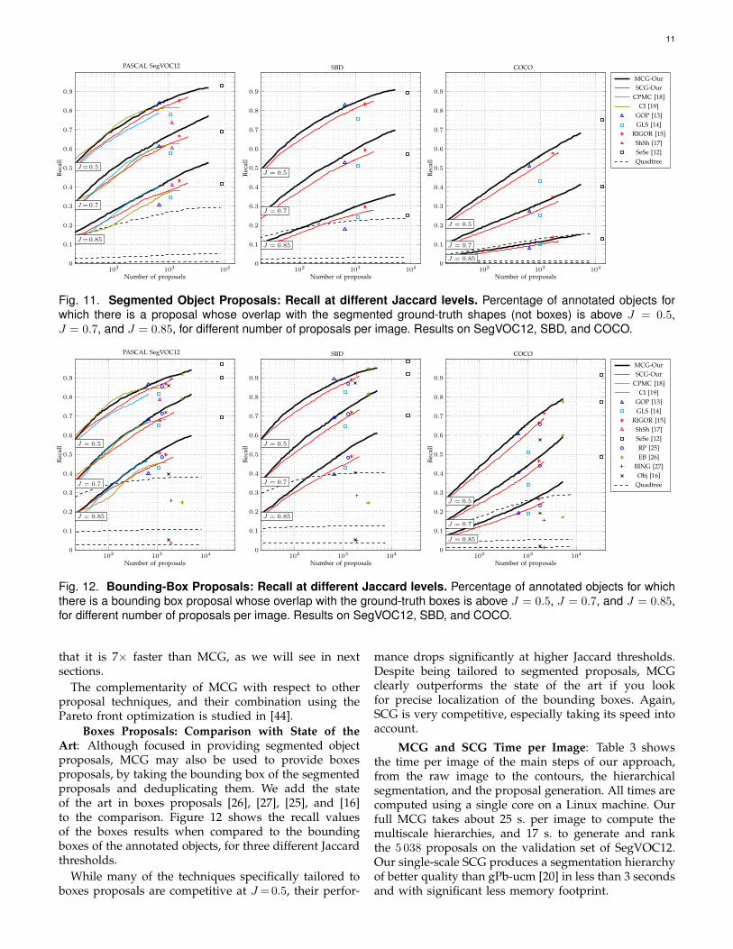
As commented on the measures description, Ji showsmean aggregate results, so they can mask the distribu-tion of quality among objects in the database. Figure 11shows the recall at three different Jaccard levels. First,these plots further highlight how challenging COCOis, since we observe a significant drop in performance,more pronounced than when measured by Ji and Jc.Another interesting result comes from observing theevolution of the plots for the three different Jaccardvalues. Take for instance the performance of GOP ( )against MCG-Our ( ) in SBD. While for J=0.5 GOPslightly outperforms MCG, the higher the threshold, thebetter MCG. Overall, MCG has specially good resultsat higher J values. In other words, if one looks forproposals of very high accuracy, MCG is the methodwith highest recall, at all regimes and in all databases.In all measures and databases, SCG ( ) obtains verycompetitive results, especially if we take into account

11

PASCAL SegVOC12

102 103 1040

0.1

0.2

0.3

0.4

0.5

0.6

0.7

0.8

0.9

J=0.5

J=0.7

J=0.85

Number of proposals

Rec

all

SBD

102 103 1040

0.1

0.2

0.3

0.4

0.5

0.6

0.7

0.8

0.9

J = 0.5

J = 0.7

J = 0.85

Number of proposals

Rec

all

COCO

102 103 1040

0.1

0.2

0.3

0.4

0.5

0.6

0.7

0.8

0.9

J = 0.5

J = 0.7

J = 0.85

Number of proposals

Rec

all

MCG-OurSCG-Our

CPMC [18]CI [19]

GOP [13]GLS [14]

RIGOR [15]ShSh [17]SeSe [12]Quadtree

Fig. 11. Segmented Object Proposals: Recall at different Jaccard levels. Percentage of annotated objects forwhich there is a proposal whose overlap with the segmented ground-truth shapes (not boxes) is above J = 0.5,J = 0.7, and J = 0.85, for different number of proposals per image. Results on SegVOC12, SBD, and COCO.

PASCAL SegVOC12

102 103 1040

0.1

0.2

0.3

0.4

0.5

0.6

0.7

0.8

0.9

J = 0.5

J = 0.7

J = 0.85

Number of proposals

Rec

all

SBD

102 103 1040

0.1

0.2

0.3

0.4

0.5

0.6

0.7

0.8

0.9

J = 0.5

J = 0.7

J = 0.85

Number of proposals

Rec

all

COCO

102 103 1040

0.1

0.2

0.3

0.4

0.5

0.6

0.7

0.8

0.9

J = 0.5

J = 0.7

J = 0.85

Number of proposals

Rec

all

MCG-OurSCG-Our

CPMC [18]CI [19]

GOP [13]GLS [14]

RIGOR [15]ShSh [17]SeSe [12]RP [25]EB [26]

BING [27]Obj [16]

Quadtree

Fig. 12. Bounding-Box Proposals: Recall at different Jaccard levels. Percentage of annotated objects for whichthere is a bounding box proposal whose overlap with the ground-truth boxes is above J = 0.5, J = 0.7, and J = 0.85,for different number of proposals per image. Results on SegVOC12, SBD, and COCO.

that it is 7× faster than MCG, as we will see in nextsections.

The complementarity of MCG with respect to otherproposal techniques, and their combination using thePareto front optimization is studied in [44].

Boxes Proposals: Comparison with State of theArt: Although focused in providing segmented objectproposals, MCG may also be used to provide boxesproposals, by taking the bounding box of the segmentedproposals and deduplicating them. We add the stateof the art in boxes proposals [26], [27], [25], and [16]to the comparison. Figure 12 shows the recall valuesof the boxes results when compared to the boundingboxes of the annotated objects, for three different Jaccardthresholds.

While many of the techniques specifically tailored toboxes proposals are competitive at J =0.5, their perfor-

mance drops significantly at higher Jaccard thresholds.Despite being tailored to segmented proposals, MCGclearly outperforms the state of the art if you lookfor precise localization of the bounding boxes. Again,SCG is very competitive, especially taking its speed intoaccount.

MCG and SCG Time per Image: Table 3 showsthe time per image of the main steps of our approach,from the raw image to the contours, the hierarchicalsegmentation, and the proposal generation. All times arecomputed using a single core on a Linux machine. Ourfull MCG takes about 25 s. per image to compute themultiscale hierarchies, and 17 s. to generate and rankthe 5 038 proposals on the validation set of SegVOC12.Our single-scale SCG produces a segmentation hierarchyof better quality than gPb-ucm [20] in less than 3 secondsand with significant less memory footprint.

12

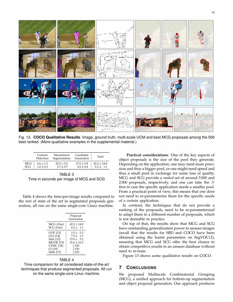
Fig. 13. COCO Qualitative Results: Image, ground truth, multi-scale UCM and best MCG proposals among the 500best ranked. (More qualitative examples in the supplemental material.)

Contour Hierarchical Candidate TotalDetection Segmentation Generation

MCG 4.6± 1.3 20.5± 5.6 17.0± 9.8 42.2± 14.8SCG 1.0± 0.3 2.7± 0.7 2.6± 0.4 6.2± 1.1

TABLE 3Time in seconds per image of MCG and SCG

Table 4 shows the time-per-image results compared tothe rest of state of the art in segmented proposals gen-eration, all run on the same single-core Linux machine.

ProposalGeneration

MCG (Our) 42.2± 14.8SCG (Our) 6.2± 1.1

GOP [13] 1.0± 0.3GLS [14] 7.9± 1.7SeSe [12] 15.9± 5.2RIGOR [15] 31.6± 16.0CPMC [18] ≥120CI [19] ≥120ShSh [17] ≥120

TABLE 4Time comparison for all considered state-of-the-art

techniques that produce segmented proposals. All runon the same single-core Linux machine.

Practical considerations: One of the key aspects ofobject proposals is the size of the pool they generate.Depending on the application, one may need more preci-sion and thus a bigger pool, or one might need speed andthus a small pool in exchange for some loss of quality.MCG and SCG provide a ranked set of around 5 000 and2 000 proposals, respectively, and one can take the Nfirst in case the specific application needs a smaller pool.From a practical point of view, this means that one doesnot need to re-parameterize them for the specific needsof a certain application.

In contrast, the techniques that do not provide aranking of the proposals, need to be re-parameterizedto adapt them to a different number of proposals, whichis not desirable in practice.

On top of that, the results show that MCG and SCGhave outstanding generalization power to unseen images(recall that the results for SBD and COCO have beenobtained using the learnt parameters on SegVOC12),meaning that MCG and SCG offer the best chance toobtain competitive results in an unseen database withoutneed to re-train.

Figure 13 shows some qualitative results on COCO.

7 CONCLUSIONS

We proposed Multiscale Combinatorial Grouping(MCG), a unified approach for bottom-up segmentationand object proposal generation. Our approach produces

13

state-of-the-art contours, hierarchical regions, and objectproposals. At its core are a fast eigenvector computationfor normalized-cut segmentation and an efficientalgorithm for combinatorial merging of hierarchicalregions. We also present Single-scale CombinatorialGrouping (SCG), a speeded up version of our techniquethat produces competitive results in under five secondsper image.

We perform an extensive validation in BSDS500,SegVOC12, SBD, and COCO, showing the quality, ro-bustness and scalability of MCG. Recently, an indepen-dent study [45], [46] provided further evidence to theinterest of MCG among the current state-of-the-art inobject proposal generation. Moreover, our object candi-dates have already been employed as integral part ofhigh performing recognition systems [47].

In order to promote reproducible research on percep-tual grouping, all the resources of this project – code,pre-computed results, and evaluation protocols – arepublicly available2.

Acknowledgements: The last iterations of this workhave been done while Jordi Pont-Tuset has been at Prof.Luc Van Gool’s Computer Vision Lab (CVL) of ETHZ,Switzerland. This work has been partly developed in theframework of the project BIGGRAPH-TEC2013-43935-Rand the FPU grant AP2008-01164; financed by the Span-ish Ministerio de Economıa y Competitividad, and the Eu-ropean Regional Development Fund (ERDF). This workwas partially supported by ONR MURI N000141010933.

REFERENCES

[1] P. Viola and M. Jones, “Robust real-time face detection,” IJCV,vol. 57, no. 2, 2004.

[2] N. Dalal and B. Triggs, “Histograms of oriented gradients forhuman detection,” in CVPR, 2005.

[3] P. Felzenszwalb, R. Girshick, D. McAllester, and D. Ramanan,“Object detection with discriminatively trained part based mod-els,” TPAMI, vol. 32, no. 9, 2010.

[4] T. Malisiewicz and A. A. Efros, “Improving spatial support forobjects via multiple segmentations,” in BMVC, 2007.

[5] C. Gu, J. Lim, P. Arbelaez, and J. Malik, “Recognition usingregions,” in CVPR, 2009.

[6] J. Carreira, F. Li, and C. Sminchisescu, “Object recognition bysequential figure-ground ranking,” IJCV, vol. 98, no. 3, pp. 243–262, 2012.

[7] A. Ion, J. Carreira, and C. Sminchisescu, “Probabilistic joint imagesegmentation and labeling by figure-ground composition,” IJCV,vol. 107, no. 1, pp. 40–57, 2014.

[8] P. Arbelaez, B. Hariharan, C. Gu, S. Gupta, L. Bourdev, andJ. Malik, “Semantic segmentation using regions and parts,” inCVPR, 2012.

[9] J. Carreira, R. Caseiro, J. Batista, and C. Sminchisescu, “Semanticsegmentation with second-order pooling,” in ECCV, 2012.

[10] R. Girshick, J. Donahue, T. Darrell, and J. Malik, “Rich featurehierarchies for accurate object detection and semantic segmenta-tion,” in CVPR, 2014.

[11] N. Zhang, J. Donahue, R. Girshick, and T. Darrell, “Part-basedr-cnns for fine-grained category detection,” in ECCV, 2014.

[12] J. R. R. Uijlings, K. E. A. van de Sande, T. Gevers, and A. W. M.Smeulders, “Selective search for object recognition,” IJCV, vol.104, no. 2, pp. 154–171, 2013.

2. www.eecs.berkeley.edu/Research/Projects/CS/vision/grouping/mcg/

[13] P. Krahenbuhl and V. Koltun, “Geodesic object proposals,” inECCV, 2014.

[14] P. Rantalankila, J. Kannala, and E. Rahtu, “Generating objectsegmentation proposals using global and local search,” in CVPR,2014.

[15] A. Humayun, F. Li, and J. M. Rehg, “RIGOR: Recycling Inferencein Graph Cuts for generating Object Regions,” in CVPR, 2014.

[16] B. Alexe, T. Deselaers, and V. Ferrari, “Measuring the objectnessof image windows,” TPAMI, vol. 34, pp. 2189–2202, 2012.

[17] J. Kim and K. Grauman, “Shape sharing for object segmentation,”in ECCV, 2012.

[18] J. Carreira and C. Sminchisescu, “CPMC: Automatic objectsegmentation using constrained parametric min-cuts,” TPAMI,vol. 34, no. 7, pp. 1312–1328, 2012.

[19] I. Endres and D. Hoiem, “Category-independent object proposalswith diverse ranking,” TPAMI, vol. 36, no. 2, pp. 222–234, 2014.

[20] P. Arbelaez, M. Maire, C. C. Fowlkes, and J. Malik, “Contourdetection and hierarchical image segmentation,” TPAMI, vol. 33,no. 5, pp. 898–916, 2011.

[21] P. F. Felzenszwalb and D. P. Huttenlocher, “Efficient graph-basedimage segmentation,” IJCV, vol. 59, p. 2004, 2004.

[22] X. Ren and L. Bo, “Discriminatively trained sparse code gradientsfor contour detection,” in NIPS, 2012.

[23] C. J. Taylor, “Towards fast and accurate segmentation,” CVPR,2013.

[24] M. Maire and S. X. Yu, “Progressive multigrid eigensolvers formultiscale spectral segmentation,” ICCV, 2013.

[25] S. Manen, M. Guillaumin, and L. Van Gool, “Prime Object Pro-posals with Randomized Prim’s Algorithm,” in ICCV, 2013.

[26] C. L. Zitnick and P. Dollar, “Edge boxes: Locating object proposalsfrom edges,” in ECCV, 2014.

[27] M.-M. Cheng, Z. Zhang, W.-Y. Lin, and P. H. S. Torr, “BING:Binarized normed gradients for objectness estimation at 300fps,”in CVPR, 2014.

[28] D. Hoiem, A. Efros, and M. Hebert, “Recovering occlusion bound-aries from an image,” IJCV, vol. 91, no. 3, pp. 328–346, 2011.

[29] Z. Ren and G. Shakhnarovich, “Image segmentation by cascadedregion agglomeration,” in CVPR, 2013.

[30] D. Weiss and B. Taskar, “Scalpel: Segmentation cascades withlocalized priors and efficient learning,” in CVPR, 2013.

[31] L. Najman and M. Schmitt, “Geodesic saliency of watershedcontours and hierarchical segmentation,” TPAMI, vol. 18, no. 12,pp. 1163–1173, 1996.

[32] P. Arbelaez, “Boundary extraction in natural images using ultra-metric contour maps,” in POCV, June 2006.

[33] D. Martin, C. Fowlkes, and J. Malik, “Learning to detect naturalimage boundaries using local brightness, color and texture cues,”TPAMI, vol. 26, no. 5, pp. 530–549, 2004.

[34] P. Dollar and C. Zitnick, “Structured forests for fast edge detec-tion,” ICCV, 2013.

[35] http://www.eecs.berkeley.edu/Research/Projects/CS/vision/grouping/resources.html.

[36] J. Pont-Tuset and F. Marques, “Supervised evaluation of imagesegmentation and object proposal techniques,” PAMI, 2015.

[37] ——, “Measures and meta-measures for the supervised evaluationof image segmentation,” in CVPR, 2013.

[38] M. Maire, S. X. Yu, and P. Perona, “Hierarchical scene annotation,”in BMVC, 2013.

[39] M. Everingham, H. Muller, and B. Thomas, “Evaluating imagesegmentation algorithms using the pareto front,” in ECCV, 2006.

[40] M. Ehrgott, Multicriteria optimization. Springer, 2005.[41] M. Everingham, L. Van Gool, C. K. I. Williams, J. Winn,

and A. Zisserman, “The PASCAL Visual Object ClassesChallenge 2012 (VOC2012) Results,” http://www.pascal-network.org/challenges/VOC/voc2012/workshop/index.html.

[42] B. Hariharan, P. Arbelaez, L. Bourdev, S. Maji, and J. Malik,“Semantic contours from inverse detectors,” in ICCV, 2011.

[43] T.-Y. Lin, M. Maire, S. Belongie, J. Hays, P. Perona, D. Ramanan,P. Dollar, and C. Zitnick, “Microsoft COCO: Common Objects inContext,” in ECCV, 2014.

[44] J. Pont-Tuset and L. V. Gool, “Boosting object proposals: Frompascal to COCO,” in ICCV, 2015.

[45] J. Hosang, R. Benenson, and B. Schiele, “How good are detectionproposals, really?” in BMVC, 2014.

[46] J. Hosang, R. Benenson, P. Dollar, and B. Schiele, “What makesfor effective detection proposals?” PAMI, 2015.

14

[47] B. Hariharan, P. Arbelaez, R. Girshick, and J. Malik, “Simultane-ous detection and segmentation,” in ECCV, 2014.

Jordi Pont-Tuset is a post-doctoral researcherat ETHZ, Switzerland, in Prof. Luc Van Gool’scomputer vision group (2015). He received thedegree in Mathematics in 2008, the degree inElectrical Engineering in 2008, the M.Sc. inResearch on Information and CommunicationTechnologies in 2010, and the Ph.D with honorsin 2014; all from the Universitat Politecnica deCatalunya, BarcelonaTech (UPC). He worked atDisney Research, Zurich (2014).

Pablo Arbelaez received a PhD with honors inApplied Mathematics from the Universite Paris-Dauphine in 2005. He was a Research Scientistwith the Computer Vision Group at UC Berke-ley from 2007 to 2014. He currently holds afaculty position at Universidad de los Andes inColombia. His research interests are in com-puter vision, where he has worked on a numberof problems, including perceptual grouping, ob-ject recognition and the analysis of biomedicalimages.

Jonathan T. Barron is a senior research sci-entist at Google, working on computer visionand computational photography. He received aPhD in Computer Science from the Universityof California, Berkeley in 2013, where he wasadvised by Jitendra Malik, and he received aHonours BSc in Computer Science from theUniversity of Toronto in 2007. His research inter-ests include computer vision, machine learning,computational photography, shape reconstruc-tion, and biological image analysis. He received

a National Science Foundation Graduate Research Fellowship in 2009,and the C.V. Ramamoorthy Distinguished Research Award in 2013.

Ferran Marques received the degree in Elec-trical Engineering and the Ph.D. from the Uni-versitat Politecnica de Catalunya, BarcelonaT-ech (UPC), where he is currently Professor atthe department of Signal Theory and Commu-nications. In the term 2002-2004, he servedas President of the European Association forSignal Processing (EURASIP). He has servedas Associate Editor of the IEEE Transactionson Image Processing (2009-2012) and as AreaEditor for Signal Processing: Image Communi-

cation, Elsevier (2010-2014). In 2011, he received the Jaume VicensVives distinction for University Teaching Quality. Currently, he servesas Dean of the Electrical Engineering School (ETSETB-TelecomBCN)at UPC. He has published over 150 conference and journal papers, 2books, and holds 4 international patents.

Jitendra Malik is Arthur J. Chick Professor inthe Department of Electrical Engineering andComputer Science at the University of Californiaat Berkeley, where he also holds appointmentsin vision science and cognitive science. He re-ceived the PhD degree in Computer Sciencefrom Stanford University in 1985. In January1986, he joined UC Berkeley as a faculty mem-ber in the EECS department where he served asChair of the Computer Science Division during2002-2006, and of the Department of EECS dur-

ing 2004-2006. Jitendra Malik’s group has worked on computer vision,computational modeling of biological vision, computer graphics andmachine learning. Several well-known concepts and algorithms arose inthis work, such as anisotropic diffusion, normalized cuts, high dynamicrange imaging, shape contexts and poselets. According to GoogleScholar, ten of his papers have received more than a thousand citationseach. He has graduated 33 PhD students. Jitendra was awarded theLonguet-Higgins Award for “A Contribution that has Stood the Test ofTime” twice, in 2007 and 2008. He is a Fellow of the IEEE and theACM, a member of the National Academy of Engineering, and a fellowof the American Academy of Arts and Sciences. He received the PAMIDistinguished Researcher Award in computer vision in 2013 and theK.S. Fu prize in 2014.