multiscale dataflow programming
TRANSCRIPT
Multiscale Dataflow Programming
Version 2014.1

Multiscale Dataflow Programming. Copyright c© Maxeler Technologies.
Version 2014.1May 19, 2014
Contact Information
Sales/general information: [email protected]
US Office
Maxeler Technologies IncPacific Business Center2225 E. Bayshore RoadPalo Alto, CA 94303, USA.Tel: +1 (650) 320-1614
UK Office
Maxeler Technologies Ltd1 Down PlaceLondon W6 9JH, UK.Tel: +44 (0) 208 762 6196
All rights reserved. The software described in this document is furnished under a license agreement.The software may be used or copied only under the terms of the license agreement. No part of thisdocument may be reproduced or transmitted in any form by any means, electronic or mechanical,including photocopying, recording, or by any information storage or retrieval system, without the writtenpermission of the copyright holder.
Maxeler Technolgies and the Maxeler Technologies logo are registered trademarks of Maxeler Tech-nologies, Inc. Other product or brand names may be trademarks or registered trademarks of theirrespective holders.
r41970

Foreword v
1 Multiscale Dataflow Computing 11.1 Dataflow versus control flow model of computation . . . . . . . . . . . . . . . . . . . 21.2 Dataflow engines (DFEs) . . . . . . . . . . . . . . . . . . . . . . . . . . . . . . . . . 31.3 System architecture . . . . . . . . . . . . . . . . . . . . . . . . . . . . . . . . . . . 4
2 The Simple Live CPU Interface (SLiC): Using .max Files 72.1 A first SLiC example . . . . . . . . . . . . . . . . . . . . . . . . . . . . . . . . . . . 72.2 Using multiple engine interfaces within a .max file . . . . . . . . . . . . . . . . . . . 92.3 Loading and executing .max files . . . . . . . . . . . . . . . . . . . . . . . . . . . . 92.4 Using multiple .max files . . . . . . . . . . . . . . . . . . . . . . . . . . . . . . . . . 92.5 SLiC Skins . . . . . . . . . . . . . . . . . . . . . . . . . . . . . . . . . . . . . . . . 10
2.5.1 Matlab . . . . . . . . . . . . . . . . . . . . . . . . . . . . . . . . . . . . . . . . 102.5.2 Python . . . . . . . . . . . . . . . . . . . . . . . . . . . . . . . . . . . . . . . 112.5.3 R . . . . . . . . . . . . . . . . . . . . . . . . . . . . . . . . . . . . . . . . . . 132.5.4 Skin Target Summary . . . . . . . . . . . . . . . . . . . . . . . . . . . . . . . . 142.5.5 Installer bindings . . . . . . . . . . . . . . . . . . . . . . . . . . . . . . . . . . 14
2.6 SLiC Interface levels . . . . . . . . . . . . . . . . . . . . . . . . . . . . . . . . . . . 18
3 Dataflow Programming: Creating .max Files 193.1 Identifying areas of code for dataflow engine implementation . . . . . . . . . . . . . . 203.2 Implementing a Kernel . . . . . . . . . . . . . . . . . . . . . . . . . . . . . . . . . . 223.3 Estimating performance of a simple dataflow program . . . . . . . . . . . . . . . . . 253.4 Conditionals in dataflow computing . . . . . . . . . . . . . . . . . . . . . . . . . . . 283.5 A Manager to combine Kernels into a DFE . . . . . . . . . . . . . . . . . . . . . . . 313.6 Compiling . . . . . . . . . . . . . . . . . . . . . . . . . . . . . . . . . . . . . . . . . 313.7 Simulating DFEs . . . . . . . . . . . . . . . . . . . . . . . . . . . . . . . . . . . . . 313.8 Building DFE configurations . . . . . . . . . . . . . . . . . . . . . . . . . . . . . . . 31
4 Getting Started 334.1 Building the examples and exercises in MaxIDE . . . . . . . . . . . . . . . . . . . . . 33
4.1.1 Import wizard . . . . . . . . . . . . . . . . . . . . . . . . . . . . . . . . . . . . 344.1.2 MaxCompiler project perspective . . . . . . . . . . . . . . . . . . . . . . . . . . 344.1.3 Building and running designs . . . . . . . . . . . . . . . . . . . . . . . . . . . . 374.1.4 Importing projects . . . . . . . . . . . . . . . . . . . . . . . . . . . . . . . . . . 37
4.2 Building the examples and exercises outside of MaxIDE . . . . . . . . . . . . . . . . 384.3 A basic kernel . . . . . . . . . . . . . . . . . . . . . . . . . . . . . . . . . . . . . . 394.4 Configuring a Manager . . . . . . . . . . . . . . . . . . . . . . . . . . . . . . . . . . 41
4.4.1 Building the .max file . . . . . . . . . . . . . . . . . . . . . . . . . . . . . . . . 424.5 Integrating with the CPU application . . . . . . . . . . . . . . . . . . . . . . . . . . . 454.6 Kernel graph outputs . . . . . . . . . . . . . . . . . . . . . . . . . . . . . . . . . . . 464.7 Analyzing resource usage . . . . . . . . . . . . . . . . . . . . . . . . . . . . . . . . 47
4.7.1 Enabling resource annotation . . . . . . . . . . . . . . . . . . . . . . . . . . . 49Exercises . . . . . . . . . . . . . . . . . . . . . . . . . . . . . . . . . . . . . . . . . . . . . 49
Multiscale Dataflow Programming i

5 Debugging 535.1 Simulation watches . . . . . . . . . . . . . . . . . . . . . . . . . . . . . . . . . . . . 545.2 Simulation and DFE printf . . . . . . . . . . . . . . . . . . . . . . . . . . . . . . . 575.3 Advanced debugging . . . . . . . . . . . . . . . . . . . . . . . . . . . . . . . . . . . 60
5.3.1 Launching MaxIDE’s debugger . . . . . . . . . . . . . . . . . . . . . . . . . . . 615.3.2 Kernel halted on input . . . . . . . . . . . . . . . . . . . . . . . . . . . . . . . 625.3.3 Kernel halted on output . . . . . . . . . . . . . . . . . . . . . . . . . . . . . . . 625.3.4 Stream status blocks . . . . . . . . . . . . . . . . . . . . . . . . . . . . . . . . 625.3.5 Debugging with MaxDebug . . . . . . . . . . . . . . . . . . . . . . . . . . . . . 64
6 Dataflow Variable Types 716.1 Primitive types . . . . . . . . . . . . . . . . . . . . . . . . . . . . . . . . . . . . . . 726.2 Composite types . . . . . . . . . . . . . . . . . . . . . . . . . . . . . . . . . . . . . 75
6.2.1 Composite complex numbers . . . . . . . . . . . . . . . . . . . . . . . . . . . . 756.2.2 Composite vectors . . . . . . . . . . . . . . . . . . . . . . . . . . . . . . . . . 78
6.3 Available dataflow operators . . . . . . . . . . . . . . . . . . . . . . . . . . . . . . . 80Exercises . . . . . . . . . . . . . . . . . . . . . . . . . . . . . . . . . . . . . . . . . . . . . 81
7 Scalar DFE Inputs and Outputs 83Exercises . . . . . . . . . . . . . . . . . . . . . . . . . . . . . . . . . . . . . . . . . . . . . 84
8 Navigating Streams of Data 878.1 Windows into streams . . . . . . . . . . . . . . . . . . . . . . . . . . . . . . . . . . 878.2 Static offsets . . . . . . . . . . . . . . . . . . . . . . . . . . . . . . . . . . . . . . . 898.3 Variable stream offsets . . . . . . . . . . . . . . . . . . . . . . . . . . . . . . . . . . 89
8.3.1 3D convolution example using variable offsets . . . . . . . . . . . . . . . . . . . 928.4 Dynamic offsets . . . . . . . . . . . . . . . . . . . . . . . . . . . . . . . . . . . . . 938.5 Comparing different types of offset . . . . . . . . . . . . . . . . . . . . . . . . . . . . 948.6 Stream hold . . . . . . . . . . . . . . . . . . . . . . . . . . . . . . . . . . . . . . . . 95
8.6.1 Stream hold example . . . . . . . . . . . . . . . . . . . . . . . . . . . . . . . . 98Exercises . . . . . . . . . . . . . . . . . . . . . . . . . . . . . . . . . . . . . . . . . . . . . 99
9 Control Flow in Dataflow Computing 1019.1 Simple counters . . . . . . . . . . . . . . . . . . . . . . . . . . . . . . . . . . . . . 1019.2 Nested loops . . . . . . . . . . . . . . . . . . . . . . . . . . . . . . . . . . . . . . . 1039.3 Advanced counters . . . . . . . . . . . . . . . . . . . . . . . . . . . . . . . . . . . . 104
9.3.1 Creating an advanced counter . . . . . . . . . . . . . . . . . . . . . . . . . . . 105Exercises . . . . . . . . . . . . . . . . . . . . . . . . . . . . . . . . . . . . . . . . . . . . . 109
10 Advanced SLiC Interface 11110.1 The lifetime of a .max file . . . . . . . . . . . . . . . . . . . . . . . . . . . . . . . . . 11110.2 Advanced Static . . . . . . . . . . . . . . . . . . . . . . . . . . . . . . . . . . . . . 112
10.2.1 Executing actions on DFEs . . . . . . . . . . . . . . . . . . . . . . . . . . . . . 11310.2.2 Holding the state of the DFE . . . . . . . . . . . . . . . . . . . . . . . . . . . . 113
10.3 Using multiple .max files . . . . . . . . . . . . . . . . . . . . . . . . . . . . . . . . . 11410.4 Running .max files on multiple DFEs . . . . . . . . . . . . . . . . . . . . . . . . . . 11410.5 Sharing DFEs . . . . . . . . . . . . . . . . . . . . . . . . . . . . . . . . . . . . . . . 115
10.5.1 Running actions on a DFE in a group . . . . . . . . . . . . . . . . . . . . . . . 11610.5.2 Engine loads . . . . . . . . . . . . . . . . . . . . . . . . . . . . . . . . . . . . 117
ii Multiscale Dataflow Programming

10.6 Advanced Dynamic . . . . . . . . . . . . . . . . . . . . . . . . . . . . . . . . . . . . 11710.6.1 Setting engine interface parameters . . . . . . . . . . . . . . . . . . . . . . . . 11710.6.2 Streaming data . . . . . . . . . . . . . . . . . . . . . . . . . . . . . . . . . . . 11810.6.3 Freeing the action set . . . . . . . . . . . . . . . . . . . . . . . . . . . . . . . . 11810.6.4 Advanced Dynamic example . . . . . . . . . . . . . . . . . . . . . . . . . . . . 11810.6.5 Setting and retrieving Kernel settings . . . . . . . . . . . . . . . . . . . . . . . 11910.6.6 Setting and reading mapped memories . . . . . . . . . . . . . . . . . . . . . . 11910.6.7 Action validation . . . . . . . . . . . . . . . . . . . . . . . . . . . . . . . . . . 11910.6.8 Groups and arrays of engines . . . . . . . . . . . . . . . . . . . . . . . . . . . 120
10.7 Engine interfaces . . . . . . . . . . . . . . . . . . . . . . . . . . . . . . . . . . . . . 12010.7.1 Adding an engine interface to a Manager . . . . . . . . . . . . . . . . . . . . . 12110.7.2 The default engine interface . . . . . . . . . . . . . . . . . . . . . . . . . . . . 12110.7.3 Ignoring unset parameters . . . . . . . . . . . . . . . . . . . . . . . . . . . . . 12210.7.4 Ignoring specific parameters . . . . . . . . . . . . . . . . . . . . . . . . . . . . 12310.7.5 Ignoring an entire Kernel . . . . . . . . . . . . . . . . . . . . . . . . . . . . . . 124
10.8 Engine interface parameters . . . . . . . . . . . . . . . . . . . . . . . . . . . . . . . 12410.8.1 Kernel settings . . . . . . . . . . . . . . . . . . . . . . . . . . . . . . . . . . . 12510.8.2 LMem settings . . . . . . . . . . . . . . . . . . . . . . . . . . . . . . . . . . . 12610.8.3 Autoloop offset parameters and distance measurements . . . . . . . . . . . . . 12610.8.4 Engine interface parameter arrays . . . . . . . . . . . . . . . . . . . . . . . . . 127
10.9 .max file constants . . . . . . . . . . . . . . . . . . . . . . . . . . . . . . . . . . . . 12710.10 Asynchronous execution . . . . . . . . . . . . . . . . . . . . . . . . . . . . . . . . . 128
10.10.1 Asynchronous execution example . . . . . . . . . . . . . . . . . . . . . . . . . 12910.11 Error handling . . . . . . . . . . . . . . . . . . . . . . . . . . . . . . . . . . . . . . . 12910.12 SLiC configuration . . . . . . . . . . . . . . . . . . . . . . . . . . . . . . . . . . . . 13110.13 Debug directories . . . . . . . . . . . . . . . . . . . . . . . . . . . . . . . . . . . . . 13210.14 SLiC Installer . . . . . . . . . . . . . . . . . . . . . . . . . . . . . . . . . . . . . . . 132
11 Controlled Inputs and Outputs 13311.1 Controlled inputs . . . . . . . . . . . . . . . . . . . . . . . . . . . . . . . . . . . . . 13311.2 Controlled outputs . . . . . . . . . . . . . . . . . . . . . . . . . . . . . . . . . . . . 13411.3 Simple controlled input example . . . . . . . . . . . . . . . . . . . . . . . . . . . . . 13411.4 Example for an input controlled by a counter . . . . . . . . . . . . . . . . . . . . . . 135Exercises . . . . . . . . . . . . . . . . . . . . . . . . . . . . . . . . . . . . . . . . . . . . . 137
12 On-chip FMem in Kernels 13912.1 Allocating, reading and writing FMem . . . . . . . . . . . . . . . . . . . . . . . . . . 140
12.1.1 Memory example . . . . . . . . . . . . . . . . . . . . . . . . . . . . . . . . . . 14012.2 Using memories as read-only tables . . . . . . . . . . . . . . . . . . . . . . . . . . . 141
12.2.1 ROM example . . . . . . . . . . . . . . . . . . . . . . . . . . . . . . . . . . . . 14112.2.2 Setting memory contents from the CPU . . . . . . . . . . . . . . . . . . . . . . 14112.2.3 Mapped ROM example . . . . . . . . . . . . . . . . . . . . . . . . . . . . . . . 142
12.3 Creating a memory port which both reads and writes . . . . . . . . . . . . . . . . . . 14312.4 Understanding memory resources . . . . . . . . . . . . . . . . . . . . . . . . . . . . 143Exercises . . . . . . . . . . . . . . . . . . . . . . . . . . . . . . . . . . . . . . . . . . . . . 143
Multiscale Dataflow Programming iii

13 Talking to CPUs, Large Memory (LMem), and other DFEs 14913.1 The Standard Manager . . . . . . . . . . . . . . . . . . . . . . . . . . . . . . . . . . 15013.2 MaxRing communication . . . . . . . . . . . . . . . . . . . . . . . . . . . . . . . . . 152
13.2.1 Example with loop-back across two chips . . . . . . . . . . . . . . . . . . . . . 15313.3 Large Memory (LMem) . . . . . . . . . . . . . . . . . . . . . . . . . . . . . . . . . . 154
13.3.1 Linear address generators . . . . . . . . . . . . . . . . . . . . . . . . . . . . . 15513.3.2 3D blocking address generators . . . . . . . . . . . . . . . . . . . . . . . . . . 15513.3.3 Large Memory (LMem) example . . . . . . . . . . . . . . . . . . . . . . . . . . 156
13.4 Building DFE configurations . . . . . . . . . . . . . . . . . . . . . . . . . . . . . . . 15813.4.1 BuildConfig objects . . . . . . . . . . . . . . . . . . . . . . . . . . . . . . . 158
Exercises . . . . . . . . . . . . . . . . . . . . . . . . . . . . . . . . . . . . . . . . . . . . . 159
A Java References 161
B On Multiscale Dataflow Research 163
SLiC API Index 168
MaxJ API Index 170
Index 173
iv Multiscale Dataflow Programming

Foreword
Frequency scaling of silicon technology came to an end about a decade ago. Before this programmerscame to expect that processors would simply double their speed every two years or so by increas-ing processor frequency rate. But with the increasing frequency came increasing power density and,ultimately, heat which proved to be a hard barrier. So while transistor density continues to increase,implementations now turn to some form of parallel processing to improve computational performance.
And there is a dramatic need for performance in many large applications: 3D imaging for geophysicsand medical analysis, financial risk analysis, air flow simulations in aerodynamics — the list is extensive.These applications often require large buildings with megawatts for power to support the computers —High Performance Computing (HPC) is an expensive proposition.
The obvious form of parallel processor is simply a replication of multiple processors starting with asingle silicon die (“multi core”) and extended to racks and racks of interconnected processor+memoryserver units. Even when the application can be expressed in a completely parallel form, this approachhas its own limitations especially accessing a common memory. The more processors used to accesscommon memory data the more likely contention develops to limit the overall speed.
Maxeler Technologies developed an alternative paradigm to parallel computing: Multiscale DataflowComputing. Dataflow computing was popularized by a number of researchers in the 1980’s, especiallyJ. B. Dennis. In the dataflow approach an application is considered as a dataflow graph of the exe-cutable actions; as soon as the operands for an action are valid, the action is executed and the result isforwarded to the next action in the graph. There are no load or store instructions as the operational nodecontains the relevant data. Creating a generalized interconnection among the action nodes proved tobe a significant limitation to dataflow realizations in the 1980’s. Over recent years the extraordinaryimprovement in transistor array density allowed emulations of the application dataflow graph. The Max-eler dataflow implementations are a generalization of the earlier work employing static, synchronousdataflow with an emphasis on data streaming. Indeed “multiscale” dataflow incorporates vector andarray processing to offer a multifaceted parallel compute platform.
Multiscale Dataflow Programming v

At the heart of Multiscale Dataflow Computing is the programming environment, described in thistutorial. While all this is loosely termed the Maxeler compiler the work is much more than a high leveltranslator. Embedded in it is the approach to writing optimized dataflow programs. There are at leastthree different optimization processes involved. The application actions are written in a dataflow graphtype form, unrolling loops, specifying actions processing a data stream. Next the dataflow from memorymust be described so that it can be properly scheduled into the dataflow engine. Finally, multipledataflow engines can be configured together in various ways for maximum application acceleration.All this is done using familiar programming vernacular such as Java type vocabulary. The essenceof the Maxeler programming approach is high performance with high productivity on the part of theprogrammer.
– Michael J. Flynn, Professor Emeritus, Stanford University
vi Multiscale Dataflow Programming

Welcome
Welcome to the Multiscale Dataflow Programming tutorial. To achieve Maximum Performance Com-puting we strive to combine optimizations on the algorithm level all the way down to the bit level. Inthis tutorial we show all the components that are at our disposal to balance computation with datamovement, control and numerics, while addressing functionality and optimizations. We will start byusing predefined dataflow programs before advancing to program Dataflow Engines with new dataflowprograms.
The source code for the examples, exercise stubs and solutions in this tutorial are provided in theMaxCompiler distribution.
Multiscale Dataflow Programming vii

Document conventions
When important concepts are introduced for the first time, they appear in bold.Italics are used for emphasis.Directories and commands are displayed in typewriter font.Variable and function names are displayed in typewriter font.Java methods and classes are shown using the following format:
DFEVar io.input(String name, DFEVar addr, DFEType type)
C function prototypes are similar:
max engine t∗ max load(max file t∗ maxfile, const char∗ engine id pattern);
Actual Java usage is shown without italics:
io .output(”output” , myRom, dfeUInt(32));
C usage is similarly without italics:
PassThrough(DATA SIZE, dataIn, dataOut);
Sections of code taken from the source of the examples appear with a border and line numbers:
1 package chap01 gettingstarted.ex1 passthrough;2 import com.maxeler.maxcompiler.v2.kernelcompiler.Kernel;3 import com.maxeler.maxcompiler.v2.kernelcompiler.KernelParameters;4 import com.maxeler.maxcompiler.v2.kernelcompiler.types.base.DFEVar;56 public class PassThroughKernel extends Kernel {7 PassThroughKernel(KernelParameters parameters) {8 super(parameters);9
10 // Input11 DFEVar x = io.input(”x” , dfeUInt(32)) ;12 // Output13 io .output(”y” , x, dfeUInt(32)) ;14 }15 }
viii Multiscale Dataflow Programming

1Multiscale Dataflow Computing
The programming language is not simply a tool with which a preconceived task or function canbe accomplished; it is an extensive basis of structure with which the imagination can interact.
– John Chowning
Maxeler’s Multiscale Dataflow Computing is a combination of traditional synchronous dataflow, vec-tor and array processors. We exploit loop level parallelism in a spatial, pipelined way, where largestreams of data flow through a sea of arithmetic units, connected to match the structure of the computetask. Small on-chip memories form a distributed register file with as many access ports as needed tosupport a smooth flow of data through the chip.
Multiscale Dataflow Computing employs dataflow on multiple levels of abstraction: the system level,the architecture level, the arithmetic level and the bit level. On the system level, multiple dataflowengines are connected to form a supercomputer. On the architecture level we decouple memory accessfrom arithmetic operations, while the arithmetic and bit levels provide opportunities to optimize therepresentation of the data and balance computation with communication.
Multiscale Dataflow Programming 1

1.1 Dataflow versus control flow model of computation
Memory
CPU
FunctionUnit
Instructions
Data/Instructions
Data
.c
Compiler
Memory Controller
Figure 1: Reuse of functional units over time in a CPU
1.1 Dataflow versus control flow model of computation
In a software application, a program’s source code is transformed into a list of instructions for a par-ticular processor (’control flow core’), which is then loaded into the memory, as shown in Figure 1.Instructions move through the processor and occasionally read or write data to and from memory. Mod-ern processors contain many levels of caching, forwarding and prediction logic to improve the efficiencyof this paradigm, however the programming model is inherently sequential and performance dependson the latency of memory accesses and the time for a CPU clock cycle.
In a dataflow program, we describe the operations and data choreography for a particular algorithm(see Figure 2). In a Dataflow Engine (DFE), data streams from memory into the processing chip wheredata is forwarded directly from one arithmetic unit (’dataflow core’) to another until the chain of process-ing is complete. Once a dataflow program has processed its streams of data, the dataflow engine canbe reconfigured for a new application in less than a second.
Each dataflow core computes only a single type of arithmetic operation (for example an addition ormultiplication) and is thus simple so thousands can fit on one dataflow engine. In a DFE processingpipeline every dataflow core computes simultaneously on neighboring data items in a stream. Unlikecontrol flow cores where operations are computed at different points in time on the same functional units(”computing in time”), a dataflow computation is laid out spatially on the chip (”computing in space”).Dependencies in a dataflow program are resolved statically at compile time.
One analogy for moving from control flow to dataflow is replacing artisans with a manufacturingmodel. In a factory each worker gets a simple task and all workers operate in parallel on streams ofcars and parts. Just as in manufacturing, dataflow is a method to scale up a computation to a largescale.
The dataflow engine structure itself represents the computation thus there is no need for instructionsper se; instructions are replaced by arithmetic units laid out in space and connected for a particular
2 Multiscale Dataflow Programming

1. Multiscale Dataflow Computing
Large Memory(LMem)
Data
Data
.java
MaxCompiler
DataflowCore
DataflowCore
DataflowCore
DataflowCore
DataflowCore
DataflowCore
DataflowCore
DataflowCore
DataflowCore
DataflowCore
Figure 2: A dataflow program in action.
data processing task. Because there are no instructions there is no need for instruction decode logic,instruction caches, branch prediction, or dynamic out-of-order scheduling. By eliminating the dynamiccontrol flow overhead, the full resources of the chip are dedicated to performing computation. At asystem level, the dataflow engine handles computation of large scale data processing while CPUsrunning Linux manage irregular and infrequent operations, IO and inter-node communication.
1.2 Dataflow engines (DFEs)
Figure 3 illustrates the architecture of a Maxeler dataflow processing system which comprises dataflowengines (DFEs) with their local memories attached by an interconnect to a CPU. Each DFE can im-plement multiple kernels, which perform computation as data flows between the CPU, DFE and itsassociated memories. The DFE has two types of memory: FMem (Fast Memory) which can store sev-eral megabytes of data on-chip with terabytes/second of access bandwidth and LMem (Large Memory)which can store many gigabytes of data off-chip.
The bandwidth and flexibility of FMem is a key reason why DFEs are able to achieve such highperformance on complex applications - for example a Vectis DFE can provide up to 10.4TB/s of FMembandwidth within in chip. Applications are able to effectively exploit the full FMem capacity becauseboth memory and computation are laid out in space so data can always be held in memory close tocomputation. This is in contrast to traditional CPU architectures with multi-level caches where only thesmallest/fastest cache memory level is close to the computational units and data is duplicated through
Multiscale Dataflow Programming 3

1.3 System architecture
the cache hierarchy.
W Effectively exploiting the DFE’s FMem is often the key to achieving maximum performance.
SLiC
MaxelerOS
Memory
CPU
Large M
emo
ry(LM
em)
Kernels
Manager
CPU Application
Dataflow Engine
Interconnect +
*+
Fast Memory(FMem)
Figure 3: Dataflow engine architecture
The dataflow engine is programmed with one or more Kernels and a Manager. Kernels implementcomputation while the Manager orchestrates data movement within the DFE. Given Kernels and aManager, MaxCompiler generates dataflow implementations which can then be called from the CPUvia the SLiC interface. The SLiC (Simple Live CPU) interface is an automatically generated interface tothe dataflow program, making it easy to call dataflow engines from attached CPUs.
The overall system is managed by MaxelerOS, which sits within Linux and also within the DataflowEngine’s manager. MaxelerOS manages data transfer and dynamic optimization at runtime.
1.3 System architecture
In a Maxeler dataflow supercomputing system, multiple dataflow engines are connected together via ahigh-bandwidth MaxRing interconnect, as shown in Figure 4. The MaxRing interconnect allows appli-cations to scale linearly with multiple DFEs in the system while supporting full overlap of communicationand computation.
4 Multiscale Dataflow Programming

1. Multiscale Dataflow Computing
MaxelerOSSLiC Memory
CPU
DFE
*+
+
CPU Application
MaxRingDFE
*+
+
DFE
*+
+
DFE
*+
+
*+
+
*+
+ MaxRing MaxRing
Large Memory(LMem)
Large Memory(LMem)
Large Memory(LMem)
Large Memory(LMem)
Figure 4: Maxeler dataflow system architecture
Multiscale Dataflow Programming 5

1.3 System architecture
6 Multiscale Dataflow Programming

2The Simple Live CPU Interface (SLiC):Using .max Files
Everything should be made as simple as possible, but no simpler.– A. Einstein
A Maxeler dataflow supercomputer consists of CPUs and Dataflow Engines (DFEs). The CPUs runexecutable files while DFEs run configuration files called .max (dot-max) files.
The .max file is loaded by a CPU program and runs on an available dataflow engine. MaxelerOSmanages the execution at runtime. Calling the Simple Live CPU (SLiC) API functions executes actionson the DFE, which include sending data streams and sets of parameters to the DFE.
2.1 A first SLiC example
To see how we can use the SLiC interface to interact with DFEs, we take the example of a three-pointmoving average .max file (we’ll see the source code for this .max file in the next chapter, section 3).
Multiscale Dataflow Programming 7

2.1 A first SLiC example
MaxelerOS
HWSWSLiC
User Input
Output
Compiler, Linker
CPUApplication
(.c, .f)
DataflowEngine
Configuration(.max)
AcceleratedApplication
(executable)
Figure 5: Software component interactions
A C implementation of the moving average would look like this:
void MovingAverageCPU(int size, float ∗dataIn, float ∗expected) {expected[0] = (dataIn[0] + dataIn [1]) / 2;for ( int i = 1; i < size−1; i++) {
expected[i] = (dataIn[ i−1] + dataIn[i ] + dataIn[ i +1]) / 3;}expected[size−1] = (dataIn[size−2] + dataIn[size−1]) / 2;
}
The .max file for our moving average example has the name MovingAverage.max and has aheader file MovingAverage.h. To use the SLiC functions in your C source code, you can either includethe .max file itself or include its accompanying header file with the same name, which is smaller andeasier to read. Figure 5 shows the interaction of the various software components to build a program.
The header file shows the functions that are available for a particular .max file. SLiC supportsmultiple levels of interface for interacting with DFEs; the most straightforward SLiC interface is calledBasic Static. The Basic Static level interface for this .max file has a single function:
23 void MovingAverage(24 int param N, /∗ number of floats in the input stream ∗/25 const float ∗instream x, /∗ constant input (does not change) ∗/26 float ∗outstream y); /∗ location of results ∗/
This function loads the .max file onto an available DFE, streams the input array into the DFE andwrites the results into the output array, returning once all the output data is written.
8 Multiscale Dataflow Programming
2. The Simple Live CPU Interface (SLiC): Using .max Files
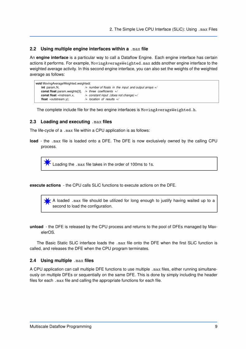
2.2 Using multiple engine interfaces within a .max file
An engine interface is a particular way to call a Dataflow Engine. Each engine interface has certainactions it performs. For example, MovingAverageWeighted.max adds another engine interface to theweighted average activity. In this second engine interface, you can also set the weights of the weightedaverage as follows:
void MovingAverageWeighted weighted(int param N, /∗ number of floats in the input and output arrays ∗/const float param weights[3], /∗ three coefficients ∗/const float ∗instream x, /∗ constant input (does not change) ∗/float ∗outstream y); /∗ location of results ∗/
The complete include file for the two engine interfaces is MovingAverageWeighted.h.
2.3 Loading and executing .max files
The life-cycle of a .max file within a CPU application is as follows:
load - the .max file is loaded onto a DFE. The DFE is now exclusively owned by the calling CPUprocess.
W Loading the .max file takes in the order of 100ms to 1s.
execute actions - the CPU calls SLiC functions to execute actions on the DFE.
W A loaded .max file should be utilized for long enough to justify having waited up to asecond to load the configuration.
unload - the DFE is released by the CPU process and returns to the pool of DFEs managed by Max-elerOS.
The Basic Static SLiC interface loads the .max file onto the DFE when the first SLiC function iscalled, and releases the DFE when the CPU program terminates.
2.4 Using multiple .max files
A CPU application can call multiple DFE functions to use multiple .max files, either running simultane-ously on multiple DFEs or sequentially on the same DFE. This is done by simply including the headerfiles for each .max file and calling the appropriate functions for each file.
Multiscale Dataflow Programming 9

2.5 SLiC Skins
Using the Basic Static SLiC interface level, each .max file is run on a different DFE. For example,imagine that we have our moving average .max file and another .max file called Threshold.max thatthresholds its input stream. Running both DFE configurations requires passing the result of the movingaverage to the thresholding DFE:
#include ”MovingAverage.h”#include ”Threshold.h”#include <MaxSLiCInterface.h>...MovingAverage(size, dataIn, mavOut);Threshold(size, mavOut, dataOut);
W To run multiple .max files on the same DFE sequentially requires using the Advanced Staticlevel (see subsection 10.2).
2.5 SLiC Skins
SLiC Skins allow Basic Static SLiC interface function calls to be made natively in languages otherthan C. Skins mean that DFE accelerated functions can be quickly integrated into applications/librarieswritten in the supported languages.
SLiC Skins are generated from .max files using the sliccompile tool bundled with MaxCompiler.sliccompile takes as one of it’s arguments the target to generate a Skin for. See Table 1 below for alist of supported targets.
Language Target Versions supportedPython python 2.4 – 2.6
MATLAB matlab R2012b or higherR R 2.11 or higher
Table 1: Supported Skin Targets
2.5.1 Matlab
The MATLAB Skin uses MATLAB objects to provide a .max file’s Basic Static SLiC interface’s function-ality. Listing 1 shows a call to the Moving Average example from MATLAB.
Listing 1: MATLAB code for executing the Moving Average kernel (MovingAverageDemo.m).1 m = MovingAverage();2 dataOut = m.default([1, 0, 2, 0, 4, 1, 8, 3]) ;3 disp(dataOut(2:7));
To create MATLAB bindings for the moving average .max file run the following command:
[user@machine]$ sliccompile -t matlab -m MovingAverage.max
10 Multiscale Dataflow Programming

2. The Simple Live CPU Interface (SLiC): Using .max Files
This creates mex MovingAverage.mexa64, MovingAverage.m and the simutils directory whichtogether comprise the MovingAverage MATLAB toolbox. When MATLAB is started from a directorycontaining these files the MovingAverage class is made available in the environment. Output argu-ments appear on the left-hand side of method calls.
Run the following command to execute the MATLAB script shown in Listing 2:
[user@machine]$ matlab movingaverage.m
Listing 2: MATLAB code for executing the Moving Average kernel (MovingAverageDemo.m).1 m = MovingAverage();2 dataOut = m.default([1, 0, 2, 0, 4, 1, 8, 3]) ;3 disp(dataOut(2:7));
The MATLAB binding creates access to Basic Static SLiC interface functions through a class namedwith the maxfile name. First create an instance of this class.
m = MovingAverage ();
This instance, m, has methods representing basic Static SLiC interface calls that are now availablethrough MATLAB. These calls keep their original names. Argument names also stay the same but outputarguments do not need to be passed as function arguments. They instead become values returned bythe functions. Some functions may return more than one item. E.g. if a Basic Static SLiC interfacefunction doSomething takes an argument a and returns arguments b and c they can be accessed asfollows:
[b, c] = m.doSomething(a);
All method documentation is available through MATLAB’s online help system. For help on a functiondoSomething belonging to the MovingAverage.max file, run
help (’MovingAverage.doSomething’)
and all input and output arguments are described.Once the object is finished with it can be removed by running the following.
clear m;
Doing this ensures all DFE connections are closed and that memory is freed.
2.5.2 Python
The Python Skin works like a normal Python module. The example in Listing 3 calculates the movingaverage of a Python list. If NumPy is installed then NumPy arrays can be used instead of Python lists.
To create Python bindings for the moving average .max file run the following command:
[user@machine]$ sliccompile -t python -m MovingAverage.max
Multiscale Dataflow Programming 11

2.5 SLiC Skins
Listing 3: Python code for executing the Moving Average kernel (MovingAverageDemo.py).1 from MovingAverage import MovingAverage2 dataOut = MovingAverage([1, 0, 2, 0, 4, 1, 8, 3])3 for i in range(len(dataOut))[1:-1]:4 print ”dataOut[%d] = %f” % (i, dataOut[i ])
This creates two files, MovingAverage.py and MovingAverage.so, and one directory namedsimutils. They encompass the Python module MovingAverage and must be kept together. To addthe module to Python’s search path start Python from the directory containing the module’s files.
The following command executes the Python program in Listing 4:
[user@machine]$ python movingaverage.py
Listing 4: Python code for executing the Moving Average kernel (MovingAverageDemo.py).1 from MovingAverage import MovingAverage2 dataOut = MovingAverage([1, 0, 2, 0, 4, 1, 8, 3])3 for i in range(len(dataOut))[1:-1]:4 print ”dataOut[%d] = %f” % (i, dataOut[i ])
Once the Python module search path is set appropriately the module can be imported into Pythonlike any other module with the command:
import MovingAverage
where MovingAverage is the .max file name. When running a simulation Python must be launched withthe generated simutils directory in the current working directory.
Online documentation is available and can be viewed for the module, MovingAverage, by running
help(MovingAverage)
All .max file constants belong to the imported module object and have the same name as definedin the engine interface. Basic Static SLiC functions are made available as functions that can be calledin the imported module and keep their original defined names. The online documentation lists themethod signatures for each of these functions. The function arguments have the same name but outputarguments appear on the left-hand side of functions as return arguments. Where a function has morethan one output argument the results are returned as a tuple. Streams in Python skin interfaces can besupplied in the form of nested Python lists or as NumPy arrays.
Nested Python Lists Python lists are suitable for small tests, quick prototypes or demos. Theyare easy to use and an attempt is made to do as much run-time checking as possible. They are notappropriate for high performance code but can be used for simple prototyping.
NumPy Arrays NumPy arrays should be used for high performance code. All NumPy array elementtypes are typed and types must match the Engine interface requirements exactly. Element types offunction arguments are specified in the online documentation. When using NumPy arrays it is importantto pass arrays of C-style contiguous memory. Arrays not in this format will work but the interface maybe considerably slower. These issues are covered in more detail below.
12 Multiscale Dataflow Programming

2. The Simple Live CPU Interface (SLiC): Using .max Files
2.5.3 R
The R Skin is installed into R as a library and data is provided using R vectors or arrays. The movingaverage example called from R is shown in Listing 5.
Listing 5: R code for executing the Moving Average kernel (MovingAverageDemo.R).1 library( ”MovingAverage”)2 dataOut <- MovingAverage(c(1, 0, 2, 0, 4, 1, 8, 3))3 for ( i in 2:7)4 cat( ’o[ ’ , i , ’ ] =’ , dataOut[i ], ’\n’)
To create R bindings for the moving average .max file run the following command:
[user@machine]$ sliccompile -t R -m MovingAverage.max
This creates MovingAverage 0.1-1 R x86 64-redhat-linux-gnu.tar.gz which is an R pack-age and a simutils directory. To install it run:
[user@machine]$ R CMD INSTALL -l . MovingAverage_0.1-1_R_x86_64-redhat-linux
-gnu.tar.gz
This directory must then be added to R’s library search path:
[user@machine]$ export R_LIBS="$(pwd):$R_LIBS"
The library can now be imported into R and run from R.
[user@machine]$ R --no-save < movingaverage.R
Listing 6: R code for executing the Moving Average kernel (MovingAverageDemo.R).1 library( ”MovingAverage”)2 dataOut <- MovingAverage(c(1, 0, 2, 0, 4, 1, 8, 3))3 for ( i in 2:7)4 cat( ’o[ ’ , i , ’ ] =’ , dataOut[i ], ’\n’)
Once in the R environment and assuming the generated library (MovingAverage) has been madeavailable to R, it can be imported with the following command.
library(MovingAverage)
This imports the MovingAverage namespace into the environment. All basic Static SLiC interfacefunctions keep their original names and are imported under this namespace. These can either becalled directly or called through the namespace. E.g. the moving average function can be called asMovingAverage or as MovingAverage::MovingAverage.
Online documentation is available for all R packages though the help command.
help(MovingAverage)
Multiscale Dataflow Programming 13

2.5 SLiC Skins
Function argument names stay the same but output arguments do not need to be passed as functionarguments. They instead become values returned by the functions. When the SLiC function returnsmore than one item R gets the items as a list. E.g. if a Basic Static SLiC interface function F takes anargument a and returns arguments b and c they can be accessed as follows:
ret_list <- MovingAverage::F(a)
result_b <- ret_list$b
result_c <- ret_list$c
WWhen testing a simulation .max file it is necessary to start and stop a simulator within R. Tostart the simulator call startSimulator and to stop the simulator call stopSimulator. Bothof these functions are exposed as part of the generated R library.
2.5.4 Skin Target Summary
WIn addition to the language bindings sliccompile will also generate a simutils directory.This directory MUST be copied into the directory the R, MATLAB or Python process is startedfrom to use simulation .max files.
All three language bindings allow interaction with DFEs by script or through interactive use. Theyall come with auto-generated documentation and have simpler interfaces than C taking advantage ofhigh-level features of these languages. Details of how to build and use the language bindings can befound in subsection 10.14.
2.5.5 Installer bindings
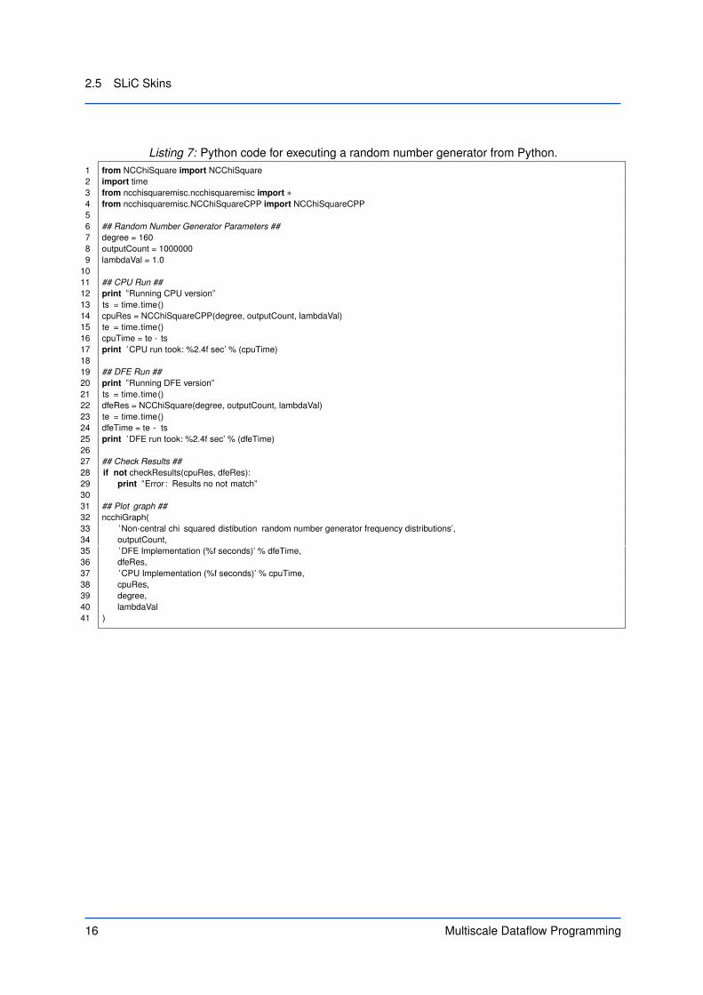
Bindings can be distributed as installer files. Installer files generate the language bindings for the skinsuser. Listing 7 shows a more complex Python example for a non-central χ2 random number generator.The Python code to interact with the DFE is simple allowing the application writer to concentrate on theapplication itself.
To import a generated Python interface use the maxfile name as the module name. All Basic StaticSLiC interface names stay the same. Functions can be imported like any other Python function.
1 from NCChiSquare import NCChiSquare
The call to the generated Python interface for the .max file is the following simple line.
22 dfeRes = NCChiSquare(degree, outputCount, lambdaVal)
All other code in the listing relates to timing, result checking and graph plotting.To unpack the demo and binding run
[user@machine]$ ./NCChiSquare_installer -t python
14 Multiscale Dataflow Programming
2. The Simple Live CPU Interface (SLiC): Using .max Files
The demo can then be executed by running
[user@machine]$ python NCChiSquareDemo.py
Figure 6 shows a screenshot of the demo application.
Multiscale Dataflow Programming 15
2.5 SLiC Skins
Listing 7: Python code for executing a random number generator from Python.1 from NCChiSquare import NCChiSquare2 import time3 from ncchisquaremisc.ncchisquaremisc import ∗4 from ncchisquaremisc.NCChiSquareCPP import NCChiSquareCPP56 ## Random Number Generator Parameters ##7 degree = 1608 outputCount = 10000009 lambdaVal = 1.0
1011 ## CPU Run ##12 print ”Running CPU version”13 ts = time.time()14 cpuRes = NCChiSquareCPP(degree, outputCount, lambdaVal)15 te = time.time()16 cpuTime = te - ts17 print ’CPU run took: %2.4f sec’ % (cpuTime)1819 ## DFE Run ##20 print ”Running DFE version”21 ts = time.time()22 dfeRes = NCChiSquare(degree, outputCount, lambdaVal)23 te = time.time()24 dfeTime = te - ts25 print ’DFE run took: %2.4f sec’ % (dfeTime)2627 ## Check Results ##28 if not checkResults(cpuRes, dfeRes):29 print ”Error: Results no not match”3031 ## Plot graph ##32 ncchiGraph(33 ’Non-central chi squared distibution random number generator frequency distributions’,34 outputCount,35 ’DFE Implementation (%f seconds)’ % dfeTime,36 dfeRes,37 ’CPU Implementation (%f seconds)’ % cpuTime,38 cpuRes,39 degree,40 lambdaVal41 )
16 Multiscale Dataflow Programming

2. The Simple Live CPU Interface (SLiC): Using .max Files
Figure 6: Non-central χ2 random number Generation demo
Multiscale Dataflow Programming 17

2.6 SLiC Interface levels
2.6 SLiC Interface levels
Overall, SLiC functionality can be accessed on three levels:
Basic Static allows a single function call to run the DFE using static actions defined for the particular.max file.
Advanced Static allows control of loading of DFEs, setting multiple complex actions, and optimizationof CPU and DFE collaboration.
Advanced Dynamic allows for the full scope of dataflow optimizations and fine-grained control of allo-cation and de-allocation of all dataflow resources.
The advanced SLiC interfaces are described in section 10.
W Non-blocking functions for all of the SLiC functions to run actions on the DFE are also availablefor all levels of the SLiC interface.
18 Multiscale Dataflow Programming

3Dataflow Programming: Creating .maxFiles
I must create a system or be enslaved by another man’s; I will not reason and compare: mybusiness is to create.
– William Blake
A dataflow application consists mostly of CPU code, with small pieces of the source code, and largeamounts of data, running on dataflow engines. We use a Java library to describe the code that runs onthe dataflow engine.
We create dataflow implementations (.max files) by writing Java code and then executing the Javacode to generate the .max file which can then be linked and called via the SLiC interface. A .max filegenerated by MaxCompiler for Maxeler DFEs comprises of two decoupled elements: Kernels and aManager. Kernels are graphs of pipelined arithmetic units. Without loops in the dataflow graph, datasimply flows from inputs to outputs. As long as there is a lot more data than there are stages in thepipeline, the execution of the computation is extremely efficient. With loops in the dataflow graph, data
Multiscale Dataflow Programming 19

3.1 Identifying areas of code for dataflow engine implementation
MaxIDE
Manager
MaxelerOS
HWSWSLiC
User Input
Output
Compiler, LinkerHardware Build
orSimulation
ManagerConfiguration
(.java)
Kernel Compiler
DataflowKernel(s)
(.java)
CPUApplication
(.c, .f)
DataflowEngine
Configuration(.max)
AcceleratedApplication
(executable)
Figure 7: MaxCompiler component interactions (blue-gray objects denote MaxCompiler components)
flows in a physical loop inside the DFE, in addition to flowing from inputs to outputs.The Manager describes the data flow choreography between Kernels, the DFE’s memory and vari-
ous available interconnects depending on the particular dataflow machine. By decoupling computationand communication, and using a flow model for off-chip I/O to the CPU, DFE interconnects and memory,Managers allow us to achieve high utilization of available resources such as arithmetic components andmemory bandwidth. Maximum performance in a Maxeler solution is achieved through a combination ofdeep-pipelining and exploiting both inter- and intra-Kernel parallelism. The high I/O-bandwidth requiredby such parallelism is supported by flexible high-performance memory controllers and a highly parallelmemory system.
MaxCompiler and MaxIDE use an extended version of Java called MaxJ which adds operator over-loading semantics to the base Java language, enabling an intuitive programming style. MaxJ sourcefiles have the .maxj file extension to differentiate them from pure Java .
Figure 7 shows the development tools provided by MaxCompiler and how they interact to build anaccelerated application.
Figure 8 shows the design flow for implementing a dataflow configuration using MaxCompiler. Thenext subsections describe each of these stages in detail.
3.1 Identifying areas of code for dataflow engine implementation
Traditionally, the first step is to analyze the application source code to determine which parts of thecode should be implemented in a dataflow engine. For Multiscale Dataflow Computing, the data ismore important than the source code. Thinking about moving data to the DFE is a much better first
20 Multiscale Dataflow Programming

3. Dataflow Programming: Creating .max Files
Design Kernels& Configure
Manager
Build and run simulation .max file
Functions Correctly?
Build and run DFE .max file
No
Yes
Meets Performance
Goals?
Yes
No
Start
End
Original Application
Identify areas of code for
acceleration
Accelerated Application
Integrate with CPU Code
Figure 8: Diagram of the design flow
Multiscale Dataflow Programming 21

3.2 Implementing a Kernel
step. Once we know which data is on the DFE at which point in time, it is obvious which pieces of codeneed to run on the DFE as well. Of course in reality this is typically an iterative process.
• The first step in creating a Multiscale Dataflow program is to measure how long it takes to run theapplication on CPUs given a set of representative (large) datasets. Limiting the analysis to toyinputs is a waste of time since CPU memory systems do not scale linearly with problem size anddataflow technology is targeting large datasets.
• Next, a more detailed analysis provides the distribution of runtime of various parts of the applica-tion including, if possible, an analysis of time spent in computation and time spent in communi-cation. Most of the analysis can be achieved with time counters and profiling tools such as gprof,oprofile, valgrind etc.
W
Acceleration is not limited to the percentage of the application that is being acceleratedbecause in real-world application development, a lot of programmer effort is spent inoptimizing the core loops while very little effort is spent on optimizing the non-criticalpieces of the application. Once the critical loops are accelerated and moved away fromthe CPUs memory system, it is typically possible to accelerate the non-critical code onthe CPU and balance the execution time on the DFE and CPUs to maximize performanceby maximizing utilization of all resources in the Multiscale Dataflow Computer.
• Maximizing regularity of computation: Dataflow engines operate best when performing the sameoperation repeatedly on many data items, for example, when computing an inner loop. To maxi-mize regularity it is imperative to consider all possible loop transformations and estimate perfor-mance of dataflow implementations for each case.
• Minimizing communication between CPU and dataflow engines: Sending/receiving data betweenthe CPU and dataflow engines is, relatively speaking, expensive since communication is usu-ally slower than computation. By carefully selecting the parts of the application to implementin a dataflow engine, we strive to overlap communication over the CPU-DFE interconnect withcomputations on both DFEs and CPUs.
The computation-to-data ratio, which describes how many mathematical operations are performedper item of data moved, is a key metric for estimating the performance of the final dataflow implemen-tation. Code that requires large amounts of data to be moved and then performs only a few arithmeticoperations poses higher balancing challenges than code with significant localized arithmetic activity.
3.2 Implementing a Kernel
In this section, we will take a detailed look at a Kernel and the implementation of the arithmetic neededwithin an algorithm. The resulting graphs of arithmetic units are the implementation of the data flowshown in Figure 2 in subsection 1.1. Kernel graphs contain a variety of different node types:
22 Multiscale Dataflow Programming

3. Dataflow Programming: Creating .max Files
Computation nodes perform arithmetic and logic operations (e.g., +,*,<,&) as well astype casts to convert between floating point, fixed point and integer variables.
Value nodes provide parameters which are either constant or set by the CPU applicationat run-time.
Stream offsets allowing access to past and future elements of data streams.
Multiplexer (mux) nodes for taking decisions.
Counter nodes for directing control flow over time, for example, keeping track of the positionin a stream for boundary calculations.
I/O nodes connecting data streams between Kernel and Manager.
Let’s consider a simple moving average example such as the one we called in the previous sectionvia the SLiC interface. The application computes a 3-point moving average over a sequence of N datavalues. At the boundaries (the beginning and the end of the data sequence), 2-point averages need tobe applied. The moving average can be expressed as:
yi =
(xi + xi+1)/2 if i = 0(xi−1 + xi)/2 if i = N−1(xi−1 + xi + xi+1)/3 otherwise
In a software implementation, an array would be used to hold the data and would be scannedthrough with a loop to compute the 3-point average for each index. The array boundaries would bechecked specifically and 2-point averages computed at these positions:
void MovingAverageSimpleCPU(int size, float ∗dataIn, float ∗expected) {expected[0] = (dataIn[0] + dataIn [1]) / 2;for ( int i = 1; i < size −1; i++) {
expected[i] = (dataIn[ i −1] + dataIn[ i ] + dataIn[ i + 1]) / 3;}expected[size −1] = (dataIn[size −2] + dataIn[size −1]) / 2;
}
The complete Java source for the implementation of this Kernel with its corresponding graph isshown in Figure 9. The arrows in the diagram show which lines of Java code generated which nodes inthe graph. The data flows from the input through the nodes in the graph to the output.
The first step in creating a dataflow kernel is to declare an input stream of the required type, in thiscase a C float type (8-bit exponent and a 24-bit mantissa):
19 DFEVar x = io.input(”x” , dfeFloat(8, 24));
Array accesses turn into accesses into a stream of data. Thus the indices of i, i − 1, and i + 1become the current, previous and next values in the input stream.
21 DFEVar prev = stream.offset(x, -1);22 DFEVar next = stream.offset(x, 1);
The average of these three values can now be calculated:
23 DFEVar sum = prev + x + next;24 DFEVar result = sum / 3;
Multiscale Dataflow Programming 23

3.2 Implementing a Kernel
y/
3
x
1+1
+ +
Figure 9: Source code for the simple moving average Kernel with the corresponding Kernel graphdiagram.
24 Multiscale Dataflow Programming

3. Dataflow Programming: Creating .max Files
Finally the result is written into an output stream:
26 io .output(”y” , result , dfeFloat(8, 24));
To demonstrate the streaming of data over time through the Kernel, Figure 10 shows a stream ofsix values passing through the Kernel. Labels have been added to show the value along the edges inthe graph. This is the programmer’s view of the data passing through the Kernel, where the actualpipelined operation of the Kernel is not considered.
W During one unit of time called a tick, the Kernel executes one step of the computation, con-sumes one input value and produces one output value.
Figure 11 shows the same six values passing through the Kernel, but this time showing how thekernel actually runs within the dataflow engine as a pipeline. This diagram makes the simplification thateach node in the graph takes a single clock cycle to produce a result, which may not always be the case,but demonstrates the principle. The graph is labeled in gray with the filling stages, when it producesno output, and the flushing stages, when it continues to produce output but consumes no input. Therelated data in the graph appears in the same color to show its progress through the pipeline.
This pipelined style of computation is key to the performance of dataflow engines, since all opera-tions can be computing in parallel on different data items within the stream. MaxCompiler automaticallymanages pipelining of the kernel so the programmer does not generally need to consider individuallatencies within the pipeline but instead can program using the abstracted view of Figure 10.
3.3 Estimating performance of a simple dataflow program
One key advantage of dataflow computing is that we can estimate the performance of the dataflowimplementation before actually implementing it, thanks to the static scheduling. For the three-pointmoving average filter above, the time to filter 1 million numbers, T , is the time for 1 million numbers toflow through the three-point filtering dataflow graph.
The first component in estimating performance in dataflow computation is the bandwidth in and outof the dataflow graph. For data in DFE memory, we simply look up the bandwidth of the particular deviceand memory storing the data. The second component is the speed at which the dataflow pipeline ismoving the data forward. A unit of time in a DFE is called a tick, and the speed of movement through adataflow pipeline is given in [ticks/second].
T = min(bandwidth, computefrequency)× 1M . Bandwidth can be thought of as the ”numbersper second“ that can be read into or written out from the DFE chip. The computefrequency is how manyticks per second the kernels can run at. The frequency is between 100-300 million ticks per secondas determined and displayed during the DFE compilation process, while bandwidth of DFEs can bebetween 200-1000 million numbers per second depending on the size of the numbers and the speed ofthe interconnect (LMEM, PCIe, Infiniband, or MaxRing).
WThe performance of the three-point filter does not depend on the computations. A 100-pointfilter runs as fast as a three point filter, as long as it fits within the resources available on theDFE. This is the essence of “computing in space” compared to “computing in time”.
Multiscale Dataflow Programming 25

3.4 Conditionals in dataflow computing
y
/
3
x
1 +1
+
+
?
?
1
?
?
0
(i) Tick 1
4 3 2 1 04 3 2 1 0
?
y
/
3
x
1 +1
+
+
0
1
2
3
1
1
(ii) Tick 2
4 3 2 1 0
? 1
y
/
3
x
1 +1
+
+
1
3
3
6
2
2
(iii) Tick 3
4 3 2 1 0
? 1 2
y
/
3
x
1 +1
+
+
2
5
4
9
3
3
(iv) Tick 4
4 3 2 1 0
? 1 2 3
y
/
3
x
1 +1
+
+
3
7
5
12
4
4
(v) Tick 5
4 3 2 1 0
? 1 2 3 4
55 5
5 5
y
/
3
x
1 +1
+
+
4
9
?
?
?
5
(vi) Tick 6
4 3 2 1 0
? 1 2 3 4
5
?
Figure 10: Programmer’s view of the simple moving average Kernel over six ticks showing the input andoutput streams.
26 Multiscale Dataflow Programming

3. Dataflow Programming: Creating .max Files
y
/
3
x
1 +1
+
+
?
?
?
?
?
0
(i) Cycle 1
4 3 2 1 04 3 2 1 0
y
/
3
x
1 +1
+
+
0
?
1
?
?
1
(ii) Cycle 2
4 3 2 1 0
y
/
3
x
1 +1
+
+
1
1
2
?
?
2
(iii) Cycle 3
4 3 2 1 0
y
/
3
x
1 +1
+
+
2
3
3
3
?
3
(iv) Cycle 4
4 3 2 1 0
y
/
3
x
1 +1
+
+
3
5
4
6
1
4
(v) Cycle 5
4 3 2 1 0
55 5
5 5
y
/
3
x
1 +1
+
+
4
7
5
9
2
5
(vi) Cycle 6
4 3 2 1 05
? ? 1 ? 1 2
y
/
3
x
1 +1
+
+
?
9
?
12
3
?
(vii) Cycle 7
4 3 2 1 05
? 1 2 3
y
/
3
x
1 +1
+
+
?
?
?
?
4
?
(viii) Cycle 8
4 3 2 1 05
? 1 2 3 4
y
/
3
x
1 +1
+
+
?
?
?
?
?
?
(ix) Cycle 9
4 3 2 1 05
? 1 2 3 4 ?
Filling Filling Filling
Flushing Flushing Flushing
Figure 11: Pipelined view of simple moving average Kernel over nine clock cycles.
Multiscale Dataflow Programming 27

3.4 Conditionals in dataflow computing
3.4 Conditionals in dataflow computing
There are three main methods of controlling conditionals that affect dataflow computation:
1. Global conditionals: These are typically large scale modes of operation depending on input pa-rameters with a relatively small number of options. If we need to select different computationsbased on input parameters, and these conditionals affect the dataflow portion of the design, wesimply create multiple .max files for each case. Some applications may require certain transfor-mation to get them into the optimal structure for supporting multiple .max files.
if (mode==1) p1(x); else p2(x);
where p1 and p2 are programs that use different .max files.
2. Local Conditionals: Conditionals depending on local state of a computation.
if (a>b) x=x+1; else x=x−1;
These can be transformed into dataflow computation as
x = (a>b) ? (x+1) : (x−1);
3. Conditional Loops: If we do not know how long we need to iterate around a loop, we need to knowa bit about the loop’s behavior and typically values for the number of loop iterations. Once weknow the distribution of values we can expect, a dataflow implementation pipelines the optimalnumber of iterations and treats each of the block of iterations as an action for the SLiC interface,controlled by the CPU (or some other kernel).
WThe ternary-if operator (?:) selects between two input streams. To select between more thantwo streams, the control.mux method is easier to use and read than nested ternary-if state-ments.
Figure 12 shows a more complex three-point average Kernel where the boundary cases are takeninto consideration.
At these boundary cases, we need to calculate the average of only two inputs. However, we cannotconditionally create a 2-input or 3-input average depending on the current position in the stream atrun-time: we must instantiate any adders and dividers at compile-time to have them implemented in thelogic of the dataflow engine. At run-time, we can choose which inputs to use for our adders and dividersto get the correct average.
In order to deal with boundaries, Figure 12 shows how the operands are provided by conditionalassignments, which are driven by a conditional expression using the ternary if operator (?:). One ofthe operands to the addition comes from a conditional assignment which selects between the previousstream value and the constant zero. Another operand is provided by the other conditional assignmentwhich selects between the next stream value and the constant zero:
36 DFEVar prev = aboveLowerBound ? prevOriginal : 0;37 DFEVar next = belowUpperBound ? nextOriginal : 0;
28 Multiscale Dataflow Programming

3. Dataflow Programming: Creating .max Files
The third operand is always the current stream value. A final conditional assignment selects be-tween a constant divisor 3 and a constant divisor of 2, depending on whether the current location is atthe boundary or not.
The left-hand part of the Kernel graph in Figure 12 shows the control logic to decide if we areat the boundary or not. We keep track of the stream position via a position counter. The methodcontrol.count.simpleCounter creates a counter and takes two parameters: the bit-width of thecounter and maximum value (in this case, size):
29 DFEVar count = control.count.simpleCounter(32, size);
The output of this counter is a stream of integer values. The counter is initialized to zero when thefirst input data value x enters the Kernel and is subsequently incremented for every newly arriving inputdata value.
W A counter in a dataflow program is equivalent to a loop variable in CPU code.
We can use standard relational and logical operators such as <, > and & to compute Boolean flagsfor the control input of a conditional assignment. In our case above, we compute a flag for the lowerboundary, a flag for the upper boundary (i < N−1) and a flag for being in-between the two boundaries:
31 DFEVar aboveLowerBound = count > 0;32 DFEVar belowUpperBound = count < size - 1;3334 DFEVar withinBounds = aboveLowerBound & belowUpperBound;
Finally, we calculate the average using the standard operators (+ and /):
41 DFEVar sum = prev + x + next;42 DFEVar result = sum / divisor ;
Multiscale Dataflow Programming 29

3.4 Conditionals in dataflow computing
y/
2
x
1+1
+ +
|
cnt
mux
01
><
&3
mux
01
mux
01
0
0N
1
cont
rol
data
Figure 12: Source code for a moving average Kernel that handles boundary cases with the correspond-ing Kernel graph diagram
30 Multiscale Dataflow Programming

3. Dataflow Programming: Creating .max Files
3.5 A Manager to combine Kernels into a DFE
Once we have our Kernels, we need to put them together in a Manager. MaxCompiler includes anumber of parameterizable Managers, some of which are general purpose while others connect Kernelstogether in optimal configurations common for specific application domains.
Once the code for Kernels and the configuration of a Manager are combined they form a completedataflow program. The execution of this program results in either the generation of a dataflow engineconfiguration file (.max file), or the execution of a DFE simulation. In either case, MaxCompiler alwaysgenerates an include file to go with a .max file.
3.6 Compiling
There are several stages to compilation in MaxCompiler as a result of being accessed as a Java library:
1. As the Kernel Compiler and the Managers are implemented in Java, the first stage is Java com-pilation. In this stage the MaxCompiler Java compiler is used to compile user code with normalJava syntax checking etc. taking place.
2. The next stages of dataflow compilation take place at Java run-time i.e. the compiled Java code(in .class files) is executed. This process encapsulates the following further compilation steps:
(a) Graph construction: In this stage user code is executed and a graph of computation isconstructed in memory based on the user calls to the Kernel Compiler API.
(b) Kernel Compiler compilation: After all the user code to describe a design has been exe-cuted the Kernel Compiler takes the generated graph, optimizes it and converts it into eithera low-level format suitable for generating a dataflow engine, or a simulation model.
(c) Back-end compilation: Generating DFE configurations including third-party tools to gen-erate the configuration files for the chip.
3.7 Simulating DFEs
Kernels and entire DFE programs can be created in a trial-and-error programming model by usingMaxeler DFE simulation. The simulator offers visibility into the execution of a Kernel and compiles inminutes rather than hours for building DFE configuration. The simulation of a DFE program runs muchmore slowly than a real implementation, so that it makes sense to first run small inputs on simulatedDFEs and then run large inputs on actual DFEs.
3.8 Building DFE configurations
Executing a Manager results in the generation of a dataflow engine configuration file with a .max exten-sion. This file contains both data used to configure the dataflow engine and meta-data used by softwareto communicate with this specific dataflow engine configuration. MaxCompiler automates the runningof third-party tools to create this configuration seamlessly. This build process can take many hours fora complex design, so simulation is recommended for early verification of the design.
Multiscale Dataflow Programming 31

3.8 Building DFE configurations
32 Multiscale Dataflow Programming

4Getting Started
All truth passes through three stages: First, it is ridiculed. Second, it is violently opposed.Third, it is accepted as being self evident.
– Schopenhauer
This section takes you through a step-by-step process to write your own dataflow program inMaxIDE, the Maxeler development environment, based on the Eclipse open source platform. In theprocess we will be creating Kernel designs, configuring Managers, building .max files for simulationand DFEs, and programming the CPU application software using the SLiC Interface.
4.1 Building the examples and exercises in MaxIDE
To launch MaxIDE, enter the command maxide at a shell command prompt. Figure 13 shows anexcerpt of the welcome page displayed when MaxIDE is launched.
Multiscale Dataflow Programming 33

4.1 Building the examples and exercises in MaxIDE
Figure 13: MaxIDE Welcome Page
4.1.1 Import wizard
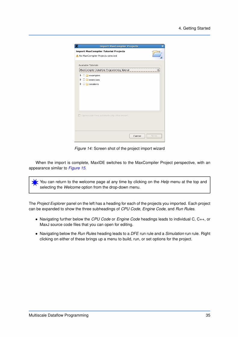
To work through the examples and exercises, you can import the project source code into MaxIDE. Clickon Auto-import MaxCompiler tutorial projects on the welcome page. This brings up the import wizardshown in Figure 14, which shows a list of project file hierarchies.
Each hierarchy listed in the import wizard dialog box corresponds to a particular tutorial document.The most important tutorials for new users are pre-selected. You can unselect any of these or chooseadditional selections using the check boxes. You can also click on the arrow to the left of each selectionto expand it. Expanding a tutorial hierarchy reveals up to three children, namely examples, exercises,and solutions:
• examples contains complete projects suitable for building just as they appear in the tutorial.
• exercises contains partially written projects for you to finish as suggested in the tutorial.
• solutions are completed versions of the exercises for you to get help or to check your work.
Each of these can be further expanded to a list of projects, which allows you to import individualprojects.
4.1.2 MaxCompiler project perspective
Click on the Finish button to import the source code and all supporting material for your selections.
34 Multiscale Dataflow Programming
4. Getting Started
Figure 14: Screen shot of the project import wizard
When the import is complete, MaxIDE switches to the MaxCompiler Project perspective, with anappearance similar to Figure 15.
W You can return to the welcome page at any time by clicking on the Help menu at the top andselecting the Welcome option from the drop-down menu.
The Project Explorer panel on the left has a heading for each of the projects you imported. Each projectcan be expanded to show the three subheadings of CPU Code, Engine Code, and Run Rules.
• Navigating further below the CPU Code or Engine Code headings leads to individual C, C++, orMaxJ source code files that you can open for editing.
• Navigating below the Run Rules heading leads to a DFE run rule and a Simulation run rule. Rightclicking on either of these brings up a menu to build, run, or set options for the project.
Multiscale Dataflow Programming 35

4.1 Building the examples and exercises in MaxIDE
Figure 15: MaxIDE with an imported project
Debug CPU Code
Run ProjectCompile Project
CurrentProject
CurrentRun Rule
Figure 16: MaxIDE buttons for building and running a project
36 Multiscale Dataflow Programming

4. Getting Started
4.1.3 Building and running designs
You can build and run projects using the buttons in the toolbar at the top of MaxIDE, as shown inFigure 16. You can select a project and run rule combination using the drop down boxes, then click oneof the buttons to build or run it.
The buttons perform the following actions:
1. Build either a simulation or DFE .max file, depending on the selected run rule.
2. This step differs for each of the buttons:
• Compile Project - compiles the CPU source code.
• Debug CPU Code - builds and runs the CPU source code in debug mode, where you canstep through the CPU code.
• Run Project - builds and runs the CPU source code in release mode.
Alternatively, a run rule can be built or run by right-clicking on it in the Project Explorer and selectingeither Build, Debug or Run.
4.1.4 Importing projects
You can import any projects, including the tutorial projects, by:
• Right-clicking in the Project Explorer window and select Import....
• Selecting Import... from the File menu.
Both methods open a dialog where you can select the type of project to import. SelectGeneral→MaxCompiler Projects into Workspace to import a MaxCompiler project, then in the nextscreen browse to the directory contain the projects you wish to import. The final screen allows you toselect the projects that you want to import.
If you are using a shared install of MaxCompiler, you might consider checking the Copy projectsinto workspace option, otherwise you will be editing the projects in situ. Finally, the Open code filesautomatically after import option will close all windows and show the CPU code, Kernel code andManager code side by side for the project, which is useful for demonstrating a project.
W Eclipse has extensive documentation and community support at http://www.eclipse.org/,which may be a helpful supplement to this tutorial.
Multiscale Dataflow Programming 37

4.2 Building the examples and exercises outside of MaxIDE
4.2 Building the examples and exercises outside of MaxIDE
Although highly recommended, MaxIDE is not required for running the examples or any other importedprojects. The source code for any project imported into MaxIDE is accessible in a directory underyour designated MaxIDE workspace directory (typically $HOME/workspace). Project directory hierar-chies are organized and named identically to the hierarchy of headings in the Project Explorer panel(without spaces). Hence, under each project subdirectory, there are sub-directories named CPUCode,EngineCode, and RunRules.
• The CPUCode directory contains C or C++ source files and header files for the project.
• The EngineCode directory contains a src subdirectory and possibly a bin subdirectory.
– The bin subdirectory stores compiled MaxJ class files, if any.
– The src subdirectory has exactly one subdirectory named after the project. This subdirec-tory contains MaxJ source code files.
• The RunRules directory contains a subdirectory named DFE and possibly a subdirectory namedSimulation, each containing automatically generated configuration files and Makefiles.
To build a project outside of MaxIDE for a DFE or simulation, navigate to the correspondingRunRules/DFE or RunRules/Simulation directory of the project hierarchy, and invoke the make utilityusing one of the automatically generated Makefiles with an optional target.
• make – with no target builds either a simulation model or a DFE configuration .max file for theapplication without running it.
• make startsim – starts a simulator if invoked from the Simulation directory and there is nosimulator already running, but has no effect if invoked in the DFE directory or when a simulator isalready running.
• make run – builds the application if necessary, and then runs it either in a DFE or in simulation,depending on the directory.
– For DFE runs, DFE hardware is needed.
– For simulation runs, an already running simulator started by make startsim is needed.
• make stopsim – invoked from the DFE directory has no effect. From the Simulation directory,it either stops a simulator if one is running, or causes an error if not.
• make runsim – is equivalent to make startsim run stopsim
38 Multiscale Dataflow Programming

4. Getting Started
4.3 A basic kernel
The basic example that we will follow throughout this section is a Kernel that takes a single input streamx and applies a simple function:
f(x) = x2 + x
The resulting stream is connected directly to the output stream y. Figure 17 shows a graphicalrepresentation of this Kernel in the form of its Kernel graph. The Kernel graph shows the flow of datafrom inputs at the top to outputs at the bottom, passing through the nodes that are created by operationswe describe within the Kernel.
y
x
*
+
Figure 17: Graph for a simple Kernel
Listing 8 shows the Java code that implements this Kernel. We will go through this code line by line.The first five lines specify the package for this example and import Java classes: Kernel,
KernelParameters and DFEVar from the MaxCompiler Java libraries:
8 package simple;9
10 import com.maxeler.maxcompiler.v2.kernelcompiler.Kernel;11 import com.maxeler.maxcompiler.v2.kernelcompiler.KernelParameters;12 import com.maxeler.maxcompiler.v2.kernelcompiler.types.base.DFEVar;
It is common to have many package imports in MaxCompiler-based programs as MaxCompiler is im-plemented as a software library. MaxIDE automatically generates these imports in most circumstances.
The Kernel class provides an entry point into Kernel development. Within the Kernel class aredirectly or indirectly a large number of Java methods for creating Kernel designs.
We can create new Kernels by extending the class Kernel:
14 class SimpleKernel extends Kernel {
Multiscale Dataflow Programming 39

4.3 A basic kernel
Listing 8: Program for the simple Kernel (SimpleKernel.maxj).1 /∗∗2 ∗ Document: MaxCompiler tutorial (maxcompiler-tutorial.pdf)3 ∗ Chapter: 4 Example: 2 Name: Simple4 ∗ MaxFile name: Simple5 ∗ Summary:6 ∗ Takes a stream and for each value x calculates xˆ2 + x.7 ∗/8 package simple;9
10 import com.maxeler.maxcompiler.v2.kernelcompiler.Kernel;11 import com.maxeler.maxcompiler.v2.kernelcompiler.KernelParameters;12 import com.maxeler.maxcompiler.v2.kernelcompiler.types.base.DFEVar;1314 class SimpleKernel extends Kernel {15 SimpleKernel(KernelParameters parameters) {16 super(parameters);1718 // Input19 DFEVar x = io.input(”x” , dfeFloat(8, 24));2021 DFEVar result = x∗x + x;2223 // Output24 io .output(”y” , result , dfeFloat(8, 24));25 }26 }
We now need to define a constructor for our new SimpleKernel class:
15 SimpleKernel(KernelParameters parameters) {
In Java, a constructor serves as an initialization function executed when an object of a class isinstantiated.
The constructor of a Kernel class needs at least one parameter, an object of classKernelParameters. In our program, we have chosen the name parameters for this object. Althoughour Kernel does not make much use of the parameters object, this object is used internally within theKernel class. For this reason, we need to pass the parameter object to the constructor of the Kernel
object. In Java, we do this using the super call:
16 super(parameters);
The code in the body of the program generates the Kernel graph shown in Figure 17.We use the method io.input to create a named input stream:
19 DFEVar x = io.input(”x” , dfeFloat(8, 24));
io.input takes two parameters. The first is a string representing the name, in this case x, by whichthe stream can be referred to when configuring a Manager (see section 13) and running the Kernel fromthe C CPU code (see subsection 4.5). The second parameter specifies the data type for the stream. Inour example we define the data type as an IEEE 754 single-precision floating point number.
The actual function is implemented intuitively using standard operators:
21 DFEVar result = x∗x + x;
40 Multiscale Dataflow Programming

4. Getting Started
We then connect the result directly to the output stream using io.output, which takes the nameof the stream, the internal stream to connect to the output and the type of the stream:
24 io .output(”y” , result , dfeFloat(8, 24));
Input and output streams are referred to as external as they are connected to the rest of the dataflowengine in a Manager. Depending on the Manager used, these external I/Os can be connected tomemory, another dataflow engine or the CPU.
4.4 Configuring a Manager
After designing the Kernel, we need to configure a Manager to connect our Kernel to the outside worldand build our design for either DFE output or simulation.
Listing 9 presents the Java code for the Manager that builds the DFE for our simple Kernel.
Listing 9: Program for building the simple dataflow example (SimpleManager.maxj).1 /∗∗2 ∗ Document: MaxCompiler tutorial (maxcompiler-tutorial.pdf)3 ∗ Chapter: 4 Example: 2 Name: Simple4 ∗ MaxFile name: Simple5 ∗ Summary:6 ∗ Manager for the simple x∗x + x kernel design.7 ∗ All IO is between the CPU and the DFE.8 ∗/9 package simple;
1011 import com.maxeler.maxcompiler.v2.build.EngineParameters;12 import com.maxeler.maxcompiler.v2.kernelcompiler.Kernel;13 import com.maxeler.maxcompiler.v2.managers.standard.Manager;14 import com.maxeler.maxcompiler.v2.managers.standard.Manager.IOType;1516 class SimpleManager {17 public static void main(String[] args) {18 EngineParameters params = new EngineParameters(args);19 Manager manager = new Manager(params);20 Kernel kernel = new SimpleKernel(manager.makeKernelParameters());21 manager.setKernel(kernel);22 manager.setIO(IOType.ALL CPU);23 manager.createSLiCinterface();24 manager.build();25 }26 }
We first specify the package and import the class Manager from the Maxeler Standard Managerslibrary:
9 package simple;1011 import com.maxeler.maxcompiler.v2.build.EngineParameters;12 import com.maxeler.maxcompiler.v2.kernelcompiler.Kernel;13 import com.maxeler.maxcompiler.v2.managers.standard.Manager;14 import com.maxeler.maxcompiler.v2.managers.standard.Manager.IOType;
We then declare a new class SimpleManager that serves as a container for our DFE build program
Multiscale Dataflow Programming 41

4.4 Configuring a Manager
and contains a main method to run the build process:
16 class SimpleManager {17 public static void main(String[] args) {
We now create an object named manager of class Manager which is a Manager that can be usedto connect Kernel streams to communicate directly with the CPU, to an inter-dataflow-engine MaxRinglink or to LMEM directly attached to the dataflow engine:
18 EngineParameters params = new EngineParameters(args);19 Manager manager = new Manager(params);
Whether the Manager is built for DFE configurations or simulation is determined by theEngineParameters object passed to the constructor.
MaxIDE passes whether or not the .max file is to be built for simulation or DFEs, as well as otherinformation, from the run rule via an environment variable that is parsed by MaxCompiler. The Managersthat we use for DFEs and simulation are identical in all other respects for this design.
We create an instance of our Kernel and pass it to the Manager:
20 Kernel kernel = new SimpleKernel(manager.makeKernelParameters());21 manager.setKernel(kernel);
For our simple example, we want all the inputs and outputs to be connected to the CPU application.We do this using the setIO method:
22 manager.setIO(IOType.ALL CPU);
A single function call builds the default SLiC interface for the CPU code:
23 manager.createSLiCinterface();
Finally, we call the build() method of the standard Manager class, which runs all the steps re-quired for building the dataflow engine, such as calling various back-end tools:
24 manager.build();
Listing 10 and Listing 11 show example console output from the build process.
4.4.1 Building the .max file
The results of the build process are the files Simple.max and Simple.h, which are copied to the runrule directory of the project by MaxIDE.
W You can view the build log for a run rule by right-clicking on the run rule in the project explorerwindow and selecting Show Build Log.
42 Multiscale Dataflow Programming

4. Getting Started
Listing 10: DFE Build Output (part 1)
1 Tue 12:28: ##########################################
2 Tue 12:28: Compiling.
3 Tue 12:28: ##########################################
45 Tue 12:28: MaxCompiler version: 2013.3.
6 Tue 12:28: Build DFE Run Rule for tutorial-chap04-example2-simplekernel
start time: Tue Feb 25 12:28:36 GMT 2014.
7 Tue 12:28: Project location: /home/user/tutorial-chap04-example2-
simplekernel.
8 Tue 12:28: Detailed build log: /home/user/workspace/tutorial-chap04-example2
-simplekernel/RunRules/DFE/build.log.
910 Tue 12:28: Compiling Engine Code.
11 Tue 12:28: MaxCompiler version: 2013.3
12 Tue 12:28: Build "Simple" start time: Tue 25 12:28:41 GMT 2014
13 Tue 12:28: Main build process running as user user on host host.maxeler.com
14 Tue 12:28: Build location: /home/user/builds/Simple_VECTIS_DFE
15 Tue 12:28: Detailed build log available in "_build.log"
16 Tue 12:28: Instantiating manager
17 Tue 12:28: Instantiating kernel "SimpleKernel"
18 Tue 12:28: Compiling manager (CPU I/O Only)
19 Tue 12:28:
20 Tue 12:28: Compiling kernel "SimpleKernel"
21 Tue 12:29: Generating input files (VHDL, netlists, CoreGen)
22 Tue 12:31: Running back-end build (12 phases)
23 Tue 12:31: (1/12) - Prepare MaxFile Data (GenerateMaxFileDataFile)
24 Tue 12:31: (2/12) - Synthesize DFE Modules (XST)
25 Tue 12:32: (3/12) - Link DFE Modules (NGCBuild)
26 Tue 12:32: (4/12) - Prepare for Resource Analysis (EDIF2MxruBuildPass)
27 Tue 12:33: (5/12) - Generate Preliminary Annotated Source Code (
PreliminaryResourceAnnotationBuildPass)
28 Tue 12:33: (6/12) - Report Resource Usage (XilinxPreliminaryResourceSummary)
Multiscale Dataflow Programming 43

4.4 Configuring a Manager
Listing 11: DFE Build Output (part 2)
1 Tue 12:33:
2 Tue 12:33: PRELIMINARY RESOURCE USAGE
3 Tue 12:33: Logic utilization: 9809 / 297600 (3.30%)
4 Tue 12:33: LUTs: 6787 / 297600 (2.28%)
5 Tue 12:33: Primary FFs: 7539 / 297600 (2.53%)
6 Tue 12:33: Multipliers (25x18): 2 / 2016 (0.10%)
7 Tue 12:33: DSP blocks: 2 / 2016 (0.10%)
8 Tue 12:33: Block memory (BRAM18): 21 / 2128 (0.99%)
9 Tue 12:33:
10 Tue 12:33: About to start chip vendor Map/Place/Route toolflow. This will
take some time.
11 Tue 12:33: For this compile, we estimate this process may take up to 30
minutes.
12 Tue 12:33: We recommend running in simulation to verify correctness before
building a DFE configuration.
13 Tue 12:33:
14 Tue 12:33: (7/12) - Prepare for Placement (NGDBuild)
15 Tue 12:33: (8/12) - Place and Route DFE (XilinxMPPR)
16 Tue 12:33: Executing MPPR with 1 cost tables and 1 threads.
17 Tue 12:33: MPPR: Starting 1 cost table
18 Tue 12:40: MPPR: Cost table 1 met timing with score 0 (best score 0)
19 Tue 12:40: (9/12) - Prepare for Resource Analysis (XDLBuild)
20 Tue 12:41: (10/12) - Generate Resource Report (XilinxResourceUsageBuildPass)
21 Tue 12:41: (11/12) - Generate Annotated Source Code (
XilinxResourceAnnotationBuildPass)
22 Tue 12:41: (12/12) - Generate MaxFile (GenerateMaxFileXilinx)
23 Tue 12:43:
24 Tue 12:43: FINAL RESOURCE USAGE
25 Tue 12:43: Logic utilization: 7563 / 297600 (2.54%)
26 Tue 12:43: LUTs: 6332 / 297600 (2.13%)
27 Tue 12:43: Primary FFs: 5845 / 297600 (1.96%)
28 Tue 12:43: Secondary FFs: 1360 / 297600 (0.46%)
29 Tue 12:43: Multipliers (25x18): 2 / 2016 (0.10%)
30 Tue 12:43: DSP blocks: 2 / 2016 (0.10%)
31 Tue 12:43: Block memory (BRAM18): 23 / 2128 (1.08%)
32 Tue 12:43:
33 Tue 12:43: MaxFile: /home/user/builds/Simple_VECTIS_DFE/results/Simple.max (
MD5Sum: 47ecae3e026eaceb661784b29e19c784)
34 Tue 12:43: Build completed: Tue Feb 25 12:43:32 GMT 2014 (took 14 mins, 51
secs)
44 Multiscale Dataflow Programming

4. Getting Started
4.5 Integrating with the CPU application
The final step in the development of a dataflow implementation is integrating the CPU application withthe SLiC Interface, the C API for communicating with the dataflow engine. Listing 12 show the CPUapplication for our simple example.
The header files for SLiC and the .max file created by the build process need to be included in thesource:
9 #include <MaxSLiCInterface.h>10 #include ”Maxfiles.h”
MaxIDE sets up an auto-generated Maxfiles.h file to include the header files for all the .max
files in your program. If you prefer you can include the header file for each one of your .max files filesmanually.
The first part of the main program code is to allocate memory for two arrays of length size, one forinput to the Kernel and one for output. The input data array is set to the values 1-size and the outputdata array is initialized to zero:
40 for( int i = 0; i < size; i++) {41 dataIn[ i ] = i + 1;42 dataOut[i] = 0;43 }
This example uses the simplest form of the SLiC Interface to the dataflow engine, which consistsof a single function. The function prototype is automatically generated by MaxCompiler from the Javasource and can be found in the header file simple.h after the .max file has been built:
void Simple(int32 t param size, // Number of items to processconst float ∗instream x, // Input stream pointerfloat ∗outstream y); // Output stream pointer
param size is the size of the input and output stream in items, where each item is a 32-bit float.instream x is a pointer to the array containing the data to stream into the DFE and outstream y is apointer to the array for the data we wish to stream back from the DFE.
W The size of the array to stream to/from the DFE must be a multiple of 16 bytes, otherwise SLiCproduces an error message.
When called, the function streams both the input data array from the CPU memory to the dataflowengine and the dataflow engine’s output back to the output data array in CPU memory:
46 Simple(size, dataIn, dataOut);
Multiscale Dataflow Programming 45

4.6 Kernel graph outputs
Once the Kernel has been run we can verify the correctness of the result:
15 for( int i=0; i < size; i++)16 {17 if (dataOut[i] != expected[i ]) {18 fprintf ( stderr , ”Output data @ %d = %1.8g (expected %1.8g)\n”,19 i , dataOut[i ], expected[i ]) ;20 status = 1;21 }22 }
4.6 Kernel graph outputs
The Kernel Compiler can generate a number of graph files representing the Kernel at various stagesduring the compilation process. You can inspect these graphs to analyze the output derived from theinput Java and debug the design.
The graphs are viewed from MaxIDE. After building the kernel you will find the graphs appear underthe RunRule that was built. Typically there are two graphs:
• Original Kernel Graph
This graph, shown in Figure 18, presents the Kernel graph before any optimization or schedulinghas taken place. This graph is the same as the one drawn in Figure 17.• Final Kernel Graph
This graph, shown in Figure 19, displays the final Kernel after scheduling and optimisation hastaken place and inputs are aligned by buffering.
Figure 18: Kernel Graph Viewer showing the Original graph for the simple Kernel in MaxIDE
46 Multiscale Dataflow Programming

4. Getting Started
Figure 19: Final graph for the simple Kernel
W To make graphs more readable, nodes created inside functions are grouped together into asingle node. Double click on the node to view the nodes inside.
4.7 Analyzing resource usage
MaxCompiler annotates your Java code with the number of DFE resources used for each line. Theseannotated files are output into a folder called src annotated in the build directory of the project, alongwith a summary report, during the build process. Another folder called src annotated preliminary
is created, which contains the initial resource estimates before any optimization.
WThe build directory is determined by your MAXCOMPILER BUILD DIR environment variable, andis unrelated to your workspace directory. Check the Build Location: message in the con-sole output at compile-time for its location.
W Resource annotation is only available for DFE configuration builds.
Multiscale Dataflow Programming 47

4.7 Analyzing resource usage
W The resource annotation folders are copied from your build directory into your RunRule folder,where they can be viewed within MaxIDE.
Figure 20: Annotated-Source Viewer showing the resource statistics for the simple Kernel in MaxIDE
Figure 20 presents the resource statistics for our simple Kernel in MaxIDE. The right-hand side ofthe listing displays the Kernel program, and the left-hand side annotates the program with the used re-sources line by line. The resources include look-up tables (LUTs), flip-flops (FFs), block RAMs (BRAMs)and DSP blocks (DSPs).
In general, LUTs and FFs are used for kernel operations such as arithmetic, DSPs are specificallyused for multiplication operations and BRAMs are used for FMem memory. Some LUTs, FFs andBRAMs are also used by MaxelerOS in the Manager.
Line 2 lists the total number of resources required by our Kernel design and shows that our simpleKernel uses 2 DSPs but no block RAMs. Line 3 shows that the design uses only 0.18% of the device’slook-up tables, 0.12% of its flip-flops and 0.10% of its DSPs. This leaves ample room for increasing theperformance by exploiting more parallelism (for example, by simply replicating the Kernel graph).
By analyzing the resources required for each code line, you can optimize the design for minimalresource requirements which increases the dataflow configuration’s performance. Furthermore, youcan gain insight into the resource trade-offs of different styles of Kernel programming.
We can see from line 27 that nearly all of the resources used by the simple Kernel are due to thearithmetic operations. The input statement takes 32 flip-flops, and the output statement takes none(lines 25 and 30).
48 Multiscale Dataflow Programming

4. Getting Started
4.7.1 Enabling resource annotation
When using MaxIDE, or any Ant scripts generated by MaxIDE, resource annotation is set up and runautomatically.
If you are using an alternative method to build your code, the MaxCompiler infrastructure must knowwhere your source code files are located on the file system. MaxCompiler uses the MAXSOURCEDIRS
environment variable to specify the directories containing source code used by your project. Thesefiles are then copied to the build directory during the build process and annotated with resource usageinformation.
The MAXSOURCEDIRS environment variable specifies one or more source code directories separatedby colons (:). For example: /home/user/src/dir1:/home/user/src/dir2.
W Each directory in MAXSOURCEDIRS must be the parent of a package directory named in thepackage declaration of a source file.
Given a source file SimpleKernel.maxj located in the directory
/home/user/workspace/tutorial chap02 example2 simple/EngineCode/src/simple
containing the declaration package simple, this example would require a value of
/home/user/workspace/tutorial chap02 example2 simple/EngineCode/src
in MAXSOURCEDIRS.
WIf you change MAXSOURCEDIRS using MaxIDE’s Run→Run Configurations. . . dialog, your set-ting is displayed in the dialog window and used. Unsetting it reverts it to the default and stopsit from being displayed.
ExercisesExercise 1: M-Fold simple Kernel
Modify the simple example Kernel (a copy of which is provided in the exercises folder for you tochange) that we have worked through in this section to work withM parallel streams. The Kernel shouldserve M independent streams as sketched in Figure 21. Replicating a single stream computation (alsocalled a pipe) within a Kernel is a common design pattern for creating dataflow engine implementations.For applications that show sufficient parallelism, mapping multiple pipes into a Kernel design greatlyincreases the dataflow engine performance.
Name the stream inputs and outputs x1, x2, ..., xM and y1, y2, ..., yM, respectively. The number ofstreams M should be passed to the Kernel program as a constructor argument.
Multiscale Dataflow Programming 49

4.7 Analyzing resource usage
y0
x0
*
+
y1
x1
*
+
yM
xM
*
+
...
Figure 21: Sketch of the M -fold simple Kernel
50 Multiscale Dataflow Programming

4. Getting Started
Listing 12: Simple CPU application (SimpleCpuCode.c).1 /∗∗2 ∗ Document: MaxCompiler tutorial (maxcompiler-tutorial.pdf)3 ∗ Chapter: 4 Example: 2 Name: Simple4 ∗ MaxFile name: Simple5 ∗ Summary:6 ∗ Takes a stream and for each value x calculates xˆ2 + x.7 ∗/8 #include <stdint.h>9 #include <MaxSLiCInterface.h>
10 #include ”Maxfiles.h”1112 int check(float ∗dataOut, float ∗expected, int size)13 {14 int status = 0;15 for( int i=0; i < size; i++)16 {17 if (dataOut[i] != expected[i ]) {18 fprintf ( stderr , ”Output data @ %d = %1.8g (expected %1.8g)\n”,19 i , dataOut[i ], expected[i ]) ;20 status = 1;21 }22 }23 return status;24 }2526 void SimpleCPU(int size, float ∗dataIn, float ∗dataOut)27 {28 for ( int i=0 ; i<size ; i++) {29 dataOut[i] = dataIn[ i ]∗dataIn[ i ] + dataIn[ i ];30 }31 }3233 float dataIn[1024];34 float dataOut[1024];35 float expected[1024];36 const int size = 1024;3738 int main()39 {40 for( int i = 0; i < size; i++) {41 dataIn[ i ] = i + 1;42 dataOut[i] = 0;43 }4445 SimpleCPU(size, dataIn, expected);46 Simple(size, dataIn, dataOut);4748 printf ( ”Running DFE.\n”);49 int status = check(dataOut, expected, size);50 if (status)51 printf ( ”Test failed .\n”) ;52 else53 printf ( ”Test passed OK!\n”);54 return status;55 }
Multiscale Dataflow Programming 51

4.7 Analyzing resource usage
52 Multiscale Dataflow Programming

5Debugging
[...] the realization came over me with full force that a good part of the remainder of my lifewas going to be spent in finding errors in my own programs.
– Maurice Wilkes
MaxCompiler offers a number of methods for debugging a design. We can debug Kernels usingwatches, simulation printf and DFE printf. Watches tell us the value of any specified DFEVar forevery tick that a Kernel is running. DFE and simulation printf allow us to print and format the printvalues explicitly from streams within the Kernel on every tick, optionally enabled via a Boolean stream.Watches and simPrintf are available in simulation only and ignored for DFE hardware runs, whereasdfePrintf are available for both simulation and DFE hardware runs.
Two more advanced methods for debugging a DFE as it is running, or after it has run, are coveredin subsection 5.3.
Multiscale Dataflow Programming 53

5.1 Simulation watches
Figure 22: MaxIDE displaying simulation watch data
5.1 Simulation watches
A watch can be added to a stream in simulation to record the value of the stream on every Kernel tick.To add a watch, we use a method of the class DFEVar called simWatch which takes a string
argument that is used to label the watch. When the Kernel is run in simulation it generates a report inCSV (comma-separated values) format, containing data for variables which have been watched.
Listing 13 shows our moving average example with watches added to several of the streams. Forexample, we can watch the input to the Kernel:
22 DFEVar x = io.input(”x” , dfeFloat(8, 24));23 x.simWatch(”x”);
We can also watch intermediate values in the middle of the computation:
38 DFEVar prev = aboveLowerBound ? prevOriginal : 0;39 prev.simWatch(”prev”);
Upon completion of the run, the CSV report can be accessed from within MaxIDE by way of the“Simulation watch data” item that appears under the associated RunRule in the Project Explorer, asseen in Figure 22.
The Simulation watch viewer can display large datasets and makes it possible to filter, searchthrough and export the data presented:
• the data may be filtered by way of a “Java expression filter” text field: boolean expressions written
54 Multiscale Dataflow Programming
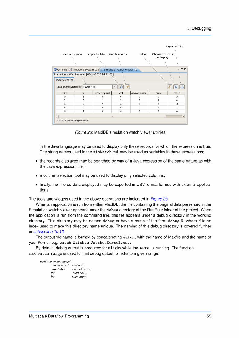
5. Debugging
Figure 23: MaxIDE simulation watch viewer utilities
in the Java language may be used to display only these records for which the expression is true.The string names used in the simWatch call may be used as variables in these expressions;
• the records displayed may be searched by way of a Java expression of the same nature as withthe Java expression filter;
• a column selection tool may be used to display only selected columns;
• finally, the filtered data displayed may be exported in CSV format for use with external applica-tions.
The tools and widgets used in the above operations are indicated in Figure 23.When an application is run from within MaxIDE, the file containing the original data presented in the
Simulation watch viewer appears under the debug directory of the RunRule folder of the project. Whenthe application is run from the command line, this file appears under a debug directory in the workingdirectory. This directory may be named debug or have a name of the form debug N, where N is anindex used to make this directory name unique. The naming of this debug directory is covered furtherin subsection 10.13.
The output file name is formed by concatenating watch with the name of Maxfile and the name ofyour Kernel, e.g. watch Watches WatchesKernel.csv.
By default, debug output is produced for all ticks while the kernel is running. The functionmax watch range is used to limit debug output for ticks to a given range:
void max watch range(max actions t ∗actions,const char ∗kernel name,int start tick ,int num ticks);
Multiscale Dataflow Programming 55

5.1 Simulation watches
Listing 13: Program for the moving average Kernel with watches (WatchesKernel.maxj).1 /∗∗2 ∗ Document: MaxCompiler Tutorial (maxcompiler-tutorial.pdf)3 ∗ Chapter: 5 Example: 1 Name: Watches4 ∗ MaxFile name: Watches5 ∗ Summary:6 ∗ Kernel that computes a three point moving average with boundaries,7 ∗ while printing watch information.8 ∗/9 package watches;
1011 import com.maxeler.maxcompiler.v2.kernelcompiler.Kernel;12 import com.maxeler.maxcompiler.v2.kernelcompiler.KernelParameters;13 import com.maxeler.maxcompiler.v2.kernelcompiler.types.base.DFEVar;1415 class WatchesKernel extends Kernel {1617 WatchesKernel(KernelParameters parameters) {18 super(parameters);1920 // Input21 DFEVar n = io.scalarInput(”n”, dfeUInt(32)) ;22 DFEVar x = io.input(”x” , dfeFloat(8, 24));23 x.simWatch(”x”);2425 // Data26 DFEVar prevOriginal = stream.offset(x, -1);27 prevOriginal .simWatch(”prevOriginal”);28 DFEVar nextOriginal = stream.offset(x, 1);2930 // Control31 DFEVar count = control.count.simpleCounter(32, n);32 count.simWatch(”cnt”);33 DFEVar aboveLowerBound = count > 0;34 DFEVar belowUpperBound = count < n - 1;35 DFEVar withinBounds = aboveLowerBound & belowUpperBound;36 aboveLowerBound.simWatch(”aboveLowerBound”);3738 DFEVar prev = aboveLowerBound ? prevOriginal : 0;39 prev.simWatch(”prev”);40 DFEVar next = belowUpperBound ? nextOriginal : 0;4142 DFEVar divisor = withinBounds ? constant.var(dfeFloat(8, 24), 3) : 2;4344 DFEVar result = (prev + x + next) / divisor ;45 result .simWatch(”result”);4647 // Output48 io .output(”y” , result , dfeFloat(8, 24));49 }5051 }
56 Multiscale Dataflow Programming

5. Debugging
Figure 24: Simulation printf output in MaxIDE
5.2 Simulation and DFE printf
simPrintf and dfePrintf behave similarly to printf in C.The basic form of a simPrintf and dfePrintf prints the formatted message to the standard
output of the application with the current value of the supplied list of objects for every tick:
void debug.simPrintf(String message, Object... args)void debug.dfePrintf(String message, Object... args)
To print the message only when a certain condition is met, a Boolean DFEVar stream can besupplied as a condition:
void debug.simPrintf(DFEVar condition, String message, Object... args)void debug.dfePrintf(DFEVar condition, String message, Object... args)
The message is only printed when condition evaluates to 1.The arguments args can contain Java variables (Byte, Short, Integer, Long, Float or Double)
or DFEVar streams. The argument message should contain corresponding format specifiers. All familiarformat specifiers from C printf are provided, with the variation that %o prints in binary, rather thanoctal.
The outputs of dfePrintf and simPrintf appear on the standard output of the application andare also saved to files upon completion of a run:
• dfePrintf produces an output file per allocated engine. These files, available in the debugdirectory, are named using the scheme debug dfeprintf.TAG.txt, where TAG is chosen to
Multiscale Dataflow Programming 57

5.2 Simulation and DFE printf
ensure that file names are unique. The outputs of dfePrintf are flushed upon deallocation ofthe engine used or, if the basic static interface is used, upon deallocation of the maxfile using theMAXFILE free() function, where MAXFILE is the name of the maxfile;
• the outputs of simPrintf are collated into a single debug printf.txt file in the debug directoryof the RunRule;
• simPrintf accepts an extra string argument NAME for outputs that should be written to a sepa-rate file:
void debug.simPrintf(String NAME, String message, Object... args)void debug.simPrintf(String NAME, DFEVar condition, String message, Object... args)
The output will then appear in a file named debug printf NAME.txt in the debug directory.
Listing 14 shows our familiar moving average example with several simPrintfs.The first simPrintf shows the current value output by the counter, which gives us the current tick
count on every Kernel tick:
30 debug.simPrintf(”Tick: %d ” , count);
The second simPrintf conditionally prints a message when the current position in the stream isin a boundary:
38 debug.simPrintf(˜withinBounds, ”[In boundary (withinBounds = %d)] ”, withinBounds);
The final simPrintf prints the result produced in the current Kernel tick:
43 debug.simPrintf(”Result: %.3g\n”, result) ;
The output from the application is shown in Listing 15.When the application is run from within MaxIDE, this output is also visible in files that appear under
the associated RunRule in the Project Explorer, upon completion of the run, as seen in figure Figure 24.The on-disk file containing the simPrintf and dfePrintf outputs, similar to watch data, is availablein a debug directory in the associated RunRule folder.
When the application is run from the command line, the output files are available in the debug
subdirectory of the current directory, or in a directory of the form debug N, where N is chosen to ensurethat this directory name is unique.
The naming of the debug directories and the configuration variables that affect it are described insubsection 10.13.
58 Multiscale Dataflow Programming

5. Debugging
Listing 14: Program for the moving average Kernel with printfs (PrintfKernel.maxj).1 /∗∗2 ∗ Document: MaxCompiler Tutorial (maxcompiler-tutorial.pdf)3 ∗ Chapter: 5 Example: 2 Name: Printf4 ∗ MaxFile name: Printf5 ∗ Summary:6 ∗ Kernel that computes a three point moving average with boundaries7 ∗ printing debug information.8 ∗/9 package printf;
1011 import com.maxeler.maxcompiler.v2.kernelcompiler.Kernel;12 import com.maxeler.maxcompiler.v2.kernelcompiler.KernelParameters;13 import com.maxeler.maxcompiler.v2.kernelcompiler.types.base.DFEVar;1415 class PrintfKernel extends Kernel {1617 PrintfKernel (KernelParameters parameters) {18 super(parameters);1920 // Input21 DFEVar n = io.scalarInput(”n”, dfeUInt(32)) ;22 DFEVar x = io.input(”x” , dfeFloat(8, 24));2324 // Data25 DFEVar prevOriginal = stream.offset(x, -1);26 DFEVar nextOriginal = stream.offset(x, 1);2728 // Control29 DFEVar count = control.count.simpleCounter(32, n);30 debug.simPrintf(”Tick: %d ” , count);31 DFEVar aboveLowerBound = count > 0;32 DFEVar belowUpperBound = count < n-1;33 DFEVar withinBounds = aboveLowerBound & belowUpperBound;3435 DFEVar prev = aboveLowerBound ? prevOriginal : 0;36 DFEVar next = belowUpperBound ? nextOriginal : 0;3738 debug.simPrintf(˜withinBounds, ”[In boundary (withinBounds = %d)] ”, withinBounds);39 DFEVar divisor = withinBounds ? constant.var(dfeFloat(8, 24), 3) : 2;4041 DFEVar result = (prev+x+next)/divisor;4243 debug.simPrintf(”Result: %.3g\n”, result) ;44 // Output45 io .output(”y” , result , dfeFloat(8, 24));46 }47 }
Listing 15: Example printf output
Tick: 0 [In boundary (withinBounds = 0)] Result: 3
Tick: 1 Result: 4
Tick: 2 Result: 6
Tick: 3 Result: 5
Tick: 4 Result: 3
Tick: 5 Result: 1
Tick: 6 Result: 4
Tick: 7 [In boundary (withinBounds = 0)] Result: 6
Multiscale Dataflow Programming 59

5.3 Advanced debugging
Launch debug mode
Figure 25: Launching a MaxCompiler project in debug mode.
5.3 Advanced debugging
Debugging with watches, simulation printf and DFE printf makes it possible to solve a rangeof issues that may appear in a design; such methods are primarily useful for inspecting the state ofkernels.
Since the Manager is a parallel and asynchronous system with many processing units, it is possibleto write control code for the CPU that leads to deadlocks such as insufficient data being either producedor consumed by the Kernels. This section presents two further tools that help to identify such issueswith the Manager and with the control software on the CPU:
• the graphical debugger in MaxIDE makes it possible to checkpoint the CPU Code of the applica-tion and inspect the state of the DFE interactively;
• the MaxDebug tool is a command line utility that obtains similar information on systems whereMaxIDE may not be present, and allows inspection of debug snapshots that are optionally pro-duced by SLiC applications as their actions are completed.
The examples in this section are based on a bitstream that performs a computation of the types = x + y, where x and y are input streams and s is an output stream, as seen in the following code
60 Multiscale Dataflow Programming

5. Debugging
Get snapshot Execute step
Stop execution
Figure 26: MaxIDE entering the debug mode.
snippet:
15 DFEVar x = io.input(”x” , type);16 DFEVar y = io.input(”y” , type);17 DFEVar sum = x + y;18 io .output(”s” , sum, type);
This Kernel expects to read one word of data from each input stream per tick, and to write oneword of data to the output stream per tick. The design malfunctions if the amount of data suppliedor consumed by the CPU does not match the number of ticks of the Kernel. The examples belowdemonstrate how to diagnose such issues in live DFEs.
5.3.1 Launching MaxIDE’s debugger
A MaxCompiler project can be launched in debug mode from within MaxIDE by pushing the debugbutton in the toolbar, or by selecting the “Debug” item in the contextual menu of a Run Rule. This isillustrated in Figure 25.
After the project has been built, MaxIDE switches to a debugging perspective and presents variousviews of the program being run, as displayed in Figure 26. This mode makes it possible to execute theprogram one instruction at a time, enabling us, in particular, to find locations where the program mightstall. At any time after a run has been launched, it is possible to obtain a snapshot of the state of theDFE by pushing the “Get snapshot” button in the debugging toolbar; this is the button with the bug icontowards the left-hand of the toolbar. MaxIDE then shows a graphical view of the Manager graph.
Multiscale Dataflow Programming 61

5.3 Advanced debugging
5.3.2 Kernel halted on input
Running the DFE or Simulation Run Rules for the example project tutorial-chap5-example3 asdistributed, results in applications that hang: the applications either fail with a timeout or need to beterminated manually by way of the red Terminate button in the console window.
WWhen running on a DFE, SLiC functions return an error when streaming operations last morethan a prescribed time; simulation does not support such time-outs, and simulated applicationswith stalling designs should be terminated manually.
Launching the application in debug mode and tracing its execution step by step allows us to seethat the function HaltedOnInput() in the CPU Code is called but does not return.
At this stage, the state of the Manager can be retrieved by pushing the snapshot button, producingthe view in Figure 27. The Kernel is represented by the yellow rectangle in the middle of the graph,surrounded by nodes that connect its inputs and outputs to the CPU.
Selecting the Kernel, by clicking with the left mouse button, indicates that its status is “Halted on
input”. In general, the yellow coloring of this state helps to locate problems in the data flow. The Kernelwould be colored green if it had run for the required number of ticks.
Examining the CPU code, we see that the number of ticks to run the Kernel has a value that is toolarge by 5000: the Kernel was running for too long and its input could not read data after size ticks.
23 HaltedOnInput(size + 5000, x, sizeBytes, y, sizeBytes, s, sizeBytes);
WNote that the current tick count in the MaxDebug output for a Kernel may not be exactly thenumber expected, given the number of inputs consumed or the number of ticks that it is set torun for, as MaxCompiler may schedule extra ticks into the Kernel.
5.3.3 Kernel halted on output
The project tutorial-chap5-example4 displays a different problem from the previous one: in thecode listing below, the size of the output stream s is now too small to accommodate the data producedby the Kernel, leading to a stall.
22 HaltedOnOutput(size, x, sizeBytes, y, sizeBytes, s, sizeBytes −5000∗sizeof(int32 t));
The result of this is shown graphically in Figure 28: the Kernel is marked as “Halted on output”and the output stream s is marked as “stalled”.
When the extra subtraction is removed, the application functions correctly; if run in the debuggerwith a breakpoint added after the call to HaltedOnOutput(), then the ensuing snapshot of the DFTshows a graph wherein each status is colored green.
5.3.4 Stream status blocks
Managers have an option to globally enable stream status blocks, which are additional blocks thatcollect information on the streams in and out of a Kernel. The status of these blocks can be read by
62 Multiscale Dataflow Programming

5. Debugging
Figure 27: State of the Manager while the function HaltedOnInput() is hanging: the Kernel requiresmore data than is available.
the debugging tools to get additional information from the DFE at run-time. See section 13 for moreinformation on Managers.
W The Manager requires rebuilding when stream status blocks are enabled, as they must be builtinto the .max file.
We can take the previous example and enable the stream status blocks using thesetEnableStreamStatusBlocks() method on the Standard Manager:
30 manager.setEnableStreamStatusBlocks(true);
For a Custom Manager, stream status blocks are enabled in the debug property of the Manager(see the “MaxCompiler Manager Compiler Tutorial” document).
The project tutorial-chap5-example5 contains a Manager with stream status enabled. Launch-ing the application in debug mode with a breakpoint after the call to DebugWithStatusBlocks(), anddisplaying the state of the DFE yields the graph in Figure 29. Selecting a stream status block by clickingin the graph displays a number of properties of the stream, including the amount of data transportedand its overall status, along with various performance-related characteristics.
Multiscale Dataflow Programming 63

5.3 Advanced debugging
Figure 28: State of the Manager while the function HaltedOnOutput() is hanging: the Kernel producesmore data than is consumed by the output stream s.
5.3.5 Debugging with MaxDebug
MaxDebug is a command line utility that makes it possible to inspect the state of a dataflow engine ina non-interactive fashion while it is running of after is has run. MaxDebug’s capabilities are as follows:
• it can obtain the status of a local hardware dataflow engine while it is running or after it has run;
• it can obtain the status of a simulated dataflow engine while it is running or after it has run, aslong as the simulated system is running;
• it can be used to display debug snapshots optionally generated by SLiC applications at the com-pletion of each action, both for local engines and engines provided by an MPC-X appliance.
To enable the tool to have this flexibility, some of its features are controlled by environment variables,and these must be modified according to the nature of the dataflow engine to be interrogated:
• for hardware dataflow engines, the environment variable MAXELEROSDIRmust point to the MaxelerOSinstallation, and the library $MAXELEROSDIR/lib/libmaxeleros.somust be preloaded by MaxDe-bug:
export LD_PRELOAD=$MAXELEROSDIR/lib/libmaxeleros.so:$LD_PRELOAD
• for simulation, the environment variable MAXCOMPILERDIR must point to the simulation librariesin the MaxCompiler installation, and the environment must be set as:
64 Multiscale Dataflow Programming

5. Debugging
Figure 29: State of the Manager after the function DebugWithStatusBlocks() has completed:stream status blocks indicate the streams’ data throughput and overall status.
export MAXELEROSDIR=$MAXCOMPILERDIR/lib/maxeleros-sim
export LD_PRELOAD=$MAXELEROSDIR/lib/libmaxeleros.so:$LD_PRELOAD
Further, in the case of simulation, the name of of the simulated engine must be specified toMaxDebug by way of the -d option. This name is based on the socket name of the simulatedsystem, which is available in the Simulator tab of the Run Rule editor of the correspondingproject.
Listing 16: MaxDebug command-line options
1 $ maxdebug
2 MaxDebug version 2014.1
34 Usage:
5 maxdebug [-v] [-g <prefix>] [-s <prefix>] [-n] [-r]
6 [-k <kernel>] [-L|-a <name>|-i <id>] [-R <mpcx>]
7 [-d <device>] [<maxfile>]
8 where:
9 -r dump scalar inputs / mapped register values
10 -m dump mapped memories
11 -g draw a manager graph annotated with runtime information
Multiscale Dataflow Programming 65

5.3 Advanced debugging
12 as a .png file for every device
13 -k <kernel> limit output to the given kernel
14 -x print all numbers in hexadecimal format
15 -v more verbose output
16 -s draw the static manager graph from the .max file
17 -d <device> use <device> when debugging the design (e.g sim0:sim,
18 /dev/maxeler0, or index if used with -a, -i or -f)
19 -f <file> file containing the maxdebug snapshot to use
20 -a <action> name of the debug snapshot to retrieve from an MPC-X
21 appliance
22 -i <id> id of the debug snapshot to retrieve from an MPC-X
23 appliance
24 -L retrieve a list of maxdebug snapshots held by an MPC-X
25 appliance
26 -R <mpcx> use <mpcx> as the IP address or hostname of an MPC-X
27 appliance
28 <maxfile> bitstream .max file (mandatory, unless -L is present)
Kernel halted on input on a simulated dataflow engine Running the Simulation Run Rules in theexample project tutorial-chap5-example3, as above, produces applications that hang. To investi-gate this problem using MaxDebug, we open a terminal, change directory to the root of the MaxCompilerproject, and set the environment for simulation:
$ export MAXELEROSDIR=$MAXCOMPILERDIR/lib/maxeleros-sim/
$ export LD_PRELOAD=$MAXELEROSDIR/lib/libmaxeleros.so:$LD_PRELOAD
We can then launch MaxDebug:
$ maxdebug -d jHaltedOnInput0:jHaltedOnInput -g graph RunRules/Simulation/
maxfiles/HaltedOnInput.max
Here, the arguments supplied to MaxDebug are:
• -d jHaltedOnInput0:jHaltedOnInput specifies the name of the engine, which is constructedas <engine-name>:<socket-name>, based on the index of the engine in the simulated systemand the socket name of the simulated system.
In this instance, the index of the engine is “0” (there being only one engine), and the socket nameof the simulated system is “jHaltedOnInput”.
For a hardware dataflow engine, this argument is not required.
• -g graph instructs MaxDebug to output an image of the state of the design. The generated filewill have “graph” as a prefix;
• RunRules/Simulation/maxfiles/HaltedOnInput.max is the path to the .max file.
The console output of this command is shown in Listing 17 and the .png file shown in Figure 30 isproduced.
66 Multiscale Dataflow Programming

5. Debugging
Listing 17: MaxDebug console output
1 MaxDebug version 2014.1
23 ============================
4 Kernel : HaltedOnInputKernel
5 ============================
67 Kernel summary
8 --------------
9 Name : HaltedOnInputKernel
10 Fill level : 10 / 10
11 Flush level : 0 / 10
12 Flushing : False
13 Ran for : 9999 / 15000 cycles
14 Derived status : Halted on input
151617 Stream summary
18 --------------
19 Name Id Type #Outstanding Reads Derived Status
20 ---- -- ---- ------------------ --------------
21 x 0 input 1 reading / no data available
22 y 1 input 1 reading / no data available
23 s 0 output writing
Multiscale Dataflow Programming 67

5.3 Advanced debugging
Figure 30: State of the Manager while the function HaltedOnInput() is hanging, as represented byMaxDebug.
68 Multiscale Dataflow Programming

5. Debugging
Saving MaxDebug snapshots for later use In the sections above, the information provided byMaxDebug was taken directly from an engine at runtime. In certain cases, we may want to save asnapshot of the content of the DFE for later use. To do this, we instruct SLiC to save a snapshotautomatically on completion of an action, by setting default maxdebug mode in the SLIC CONF envi-ronment variable:
$ env SLIC_CONF="default_maxdebug_mode=MAX_DEBUG_ALWAYS" ./HaltedOnInput
In SLiC’s dynamic interface, the same result can be achieved on a per-action basis:
void max set debug(max actions t ∗actions,const char ∗name,max debug mode t debug mode);
where the enum debug mode must be one of:
• MAX DEBUG NEVER: where no debug snapshot should be saved for the action;
• MAX DEBUG ON ERROR: where a debug snapshot should only be saved in case of stall;
• MAX DEBUG ALWAYS: where SLiC should always produce a debug snapshot;
and where name is used to identify the snapshot.In SLiC’s basic and advanced static interfaces, the MaxFile stem is used as the name of the snap-
shot.On completion of the actions, the debug snapshots are saved in the default debug directory with
file names of the form “maxdebug NAME.TIMETAG”, where NAME is the parameter specified in the callto max set debug or the MaxFile stem name, and where TIMETAG is a timestamp used to make thefile unique. These snapshots may be examined by the maxdebug command, using an additional -f<file> flag to specify the snapshot file to use, for example:
$ maxdebug -r -f <snapshot> <maxfile>
Where arrays of engines are used, the content of a specific engine may be obtained by using the-d <index> option, where the index ranges between 0 and N − 1 for an array of N devices.
Multiscale Dataflow Programming 69

5.3 Advanced debugging
70 Multiscale Dataflow Programming

6Dataflow Variable Types
A Type is defined as the range of significance of a [...] function.– Bertrand Russell, Logic and Knowledge, 1971
Variables in a dataflow program are in fact portals through which streams of numbers pass while be-ing represented in a specific way by zeros and ones. Contrary to CPUs, a multiscale dataflow computerallows us to use zeros and ones in any way we like (or don’t like) to represent the number. “Multiscale”dataflow computing means that if necessary, one can extend the optimizations and numerical algorithmdesign all the way to the bit level. For example, a loop variable that goes from 0 to 100 only really needs7 bits.
Luckily, MaxCompiler can infer most variables, and initially, an implementation only needs to declareinput variables. MaxCompiler uses the declarations of input and output variables to generate the SLiCinterface for the Kernel implementation. The basic type for any other variable is DFEVar.
From an algorithmic perspective, any variable in a program has a range and precision require-ments. From a practical perspective, we are used to assigning standard types such as int, float, anddouble to variables in our calculations. Consequently, MaxCompiler offers DFEInt and DFEFloat,corresponding to matching variable declarations in the resulting SLiC interface.
Multiscale Dataflow Programming 71

6.1 Primitive types
KernelType
DFEComplexType DFEArrayType
DFEFix DFEFloatDFEUntypedConst
KernelTypeVectorizable
DFEStructType
DFERawBits
DFEType DFEVectorBaseType
DFEVectorType
dfeUInt
dfeInt
dfeBool
Figure 31: Class hierarchy for data types
Figure 31 gives an overview of the class hierarchy for data types used in the Kernel Compiler. Thereare two categories of Kernel types within the Kernel Compiler:
Primitive types (for example DFEFloat) inherit from DFEType and can be used with DFEVar variablesas we have seen in previous chapters.
Composite types (for example DFEComplexType) do not extend DFEType: these internally translateoperations into operations on multiple DFEVar variables.
MaxCompiler and MaxIDE use an extended version of Java called MaxJ which adds operator over-loading semantics to the base Java language. This enables an intuitive programming style, for examplewith arithmetic expressions including DFEVar objects being possible. MaxJ source files have the .maxj
file extension to differentiate them from pure Java .
6.1 Primitive types
Every DFEVar instance has an associated representation type which is represented by a DFEType
object. These DFEType objects are usually assigned automatically by the Kernel Compiler or you canspecify them through casting or specification of I/O types. You can query the type of a DFEVar objectat any point using the DFEVar.getType method.
When it is necessary to explicitly specify a type for DFEVar, for example when creating an input oroptimizing a component, instances of DFEType are created indirectly using one of the following methodswhich are available from the Kernel class:
• dfeFloat(int exponent bits, int mantissa bits)
Creates a floating-point type parameterized with mantissa and exponent bit-widths. With 8 expo-nent bits and 24 mantissa bits, the format is equivalent to single-precision floating point. Similarlydouble-precision has an exponent of 11 bits and a mantissa of 53 bits.
• dfeFixOffset(int num bits, int offset, SignMode sign mode)
Creates a fixed-point type with parameterizable size and binary point offset and a choice of un-signed (SignMode.UNSIGNED) or two’s complement (SignMode.TWOSCOMPLEMENT) modes fornumber representation.
72 Multiscale Dataflow Programming

6. Dataflow Variable Types
Listing 18: Kernel demonstrating types and type casting (TypeCastKernel.maxj).1 /∗∗2 ∗ Document: MaxCompiler Tutorial (maxcompiler-tutorial.pdf)3 ∗ Chapter: 6 Example: 1 Name: Typecast4 ∗ MaxFile name: TypeCast5 ∗ Summary:6 ∗ Kernel that casts from an unsigned int to a float and back.7 ∗/89 package typecast;
1011 import com.maxeler.maxcompiler.v2.kernelcompiler.Kernel;12 import com.maxeler.maxcompiler.v2.kernelcompiler.KernelParameters;13 import com.maxeler.maxcompiler.v2.kernelcompiler.types.base.DFEFloat;14 import com.maxeler.maxcompiler.v2.kernelcompiler.types.base.DFEVar;1516 class TypeCastKernel extends Kernel {1718 TypeCastKernel(KernelParameters parameters) {19 super(parameters);2021 // Type declarations22 DFEFloat singleType = dfeFloat(8, 24); // useful : makes it easy to change types consistently2324 // Input25 DFEVar a = io.input(”a”, dfeUInt(8)) ;26 DFEVar x = io.input(”x” , singleType);2728 // Cast input ’a’ from unsigned 8-bit integer to29 // IEEE single precision float using named type,30 // then add 10.531 DFEVar result = a.cast(singleType) + 10.5;3233 // Cast input ’x’ from IEEE single precision float34 // to unsigned 8-bit integer using explicit type35 DFEVar x int = x.cast(dfeUInt(8)) ;3637 // Output38 io .output(”b”, result , singleType);39 io .output(”y” , x int , dfeUInt(8)) ;40 }4142 }
• dfeUInt(int bits)
An alias for dfeFixOffset(bits, 0, SignMode.UNSIGNED).
• dfeInt(int bits)
An alias for dfeFixOffset(bits, 0, SignMode.TWOSCOMPLEMENT).
• dfeBool()
An alias for dfeFixOffset(1, 0, SignMode.UNSIGNED). dfeBool can safely be used for allBoolean operations with numeric values 1 and 0 representing true or false respectively.
• dfeRawBits()
A Kernel type representing a binary word of user-defined length which does not have a specificKernel data type. DFERawBits streams are used to prevent invalid operations being performedinadvertently on collections of bits for which operator rules are not valid. For example, it is invalidto apply any floating-point operation to the result of DFEVar.slice. Streams of DFERawBits can
Multiscale Dataflow Programming 73

6.1 Primitive types
be cast to any other type of the same bit-width with no overhead.
The dataflow program in Listing 18 defines a number of primitive-type streams and operationson their data types. The example creates an input stream and specifies its data type by callingdfeUInt(8):
25 DFEVar a = io.input(”a”, dfeUInt(8)) ;
This dfeUInt method call creates and returns an object of class DFEFix, which directs the inputmethod to create a DFEVar object for this input with a type of unsigned 8-bit integer.
Developers may explicitly change the type of data as it flows through the graph using type casts.Type casts are typically used to change number representations as variables are reused in a dataflowprogram. Type casts are introduced by calling the cast method on DFEVar instances, for example:
35 DFEVar x int = x.cast(dfeUInt(8)) ;
In addition to integers and floating point numbers, multiscale dataflow also supports fixed pointnumbers (DFEFix). Fixed point numbers allow us to store fractions and for small range are a lot moreefficient than floating point numbers. The main drawback of fixed point numbers is that the algorithmdesigner has to think through range and precision requirements on the variables, and consider thedistribution of values for a particular variable very carefully. For iterating algorithms it is also necessaryto occasionally re-normalize the values to avoid dealing with a large range of values.
WType-casting operations, particularly those converting between floating and fixed point types,can be costly in terms of resource usage. The use of type casts should therefore be minimized.
To avoid unexpectedly large designs, MaxCompiler does not automatically infer type casts but ratherinsists that type casting be used explicitly where necessary. For example, adding a floating point numberto a fixed point number leads to a compilation error and prompts you to explicitly cast one input type tomatch the other.
WWhen casting between a floating-point number and an integer, MaxCompiler rounds to thenearest integer. This is different to the behavior in many other programming languages (suchas C/C++, Java and Fortran), where the floating-point number is truncated.
Users need to also be aware that whenever constants are used in a Kernel design without anexplicit type, the Kernel Compiler assigns these constants a type of DFEUntypedConst. An example ofan untyped constant can be seen in the example:
31 DFEVar result = a.cast(singleType) + 10.5;
This DFEUntypedConst type also propagates forward through the Kernel graph until the type foran operation can be determined. In the example, the addition operator works with the DFEVar called a,which is cast to a type of single precision floating-point. In this case the value 10.5 is also interpretedas a single-precision floating-point number. In some situations, a Kernel design may use an untypedconstant in a context where it is not possible to determine the types to use and it is not possible to
74 Multiscale Dataflow Programming

6. Dataflow Variable Types
forward-propagate the untyped constant type. For example, with a conditional assignment where bothoptions are constants we get a compile-time error until at least one of the inputs is explicitly given atype.
6.2 Composite types
While DFEVar and DFEType provide the fundamental design elements needed to create Kernel designs,more succinct solutions can often be made using composite constructs.
The composite types available in the Kernel Compiler are DFEComplexType, DFEVectorType,and DFEStructType.
6.2.1 Composite complex numbers
Listing 19 shows a Kernel design that takes in two complex numbers, adds them together and multipliesthe result by the real number 3.
A complex number type is defined to be used throughout the design using an DFEFloat objectreturned from a dfeFloat call:
16 public DFEComplexType cplxType =17 new DFEComplexType(dfeFloat(8,24));
This declares that the real and imaginary parts for instances of complex numbers created with thistype are to be stored as floating-point numbers. We could equally have used more or fewer bits for ourfloating-point type or a DFEFix type.
This type is used to specify the types of the inputs and output:
23 DFEComplex cplxIn1 = io.input(”cplxIn1”, cplxType);24 DFEComplex cplxIn2 = io.input(”cplxIn2”, cplxType);
29 io .output(”cplxOut”, result , cplxType);
In order to actually refer to our complex variables we use Java objects of type DFEComplex. TheDFEComplex class is conceptually paired with the DFEComplexType class in the same way that DFEVar
and DFEType are paired.DFEComplex type supports the familiar multiplication, subtraction and addition operators:
26 DFEComplex result = (cplxIn1 + cplxIn2) ∗ 3;
In order to run the example on a DFE, we stream the data into the dataflow engine in the correctformat. The is done as a continuous stream of single-precision floating-point numbers. Pairs of floating-point numbers are interpreted as real followed by imaginary parts.
In the CPU code for this example (Listing 20), two streams of complex numbers are initialized andstreamed to the dataflow engine. The first stream contains the complex numbers {(1 + 2i), (3 +
4i)} and the second stream contains {(5 + 6i), (7 + 8i)}:50 float cplxIn1 [] = {51 1, 2, // ( real , imaginary)52 3, 4 };5354 float cplxIn2 [] = { 5, 6, 7, 8 };
Multiscale Dataflow Programming 75

6.2 Composite types
Listing 19: Kernel demonstrating complex number support (ComplexKernel.maxj).1 /∗∗2 ∗ Document: MaxCompiler Tutorial (maxcompiler-tutorial.pdf)3 ∗ Chapter: 6 Example: 2 Name: Complex4 ∗ MaxFile name: Complex5 ∗ Summary:6 ∗ Kernel that performs complex arithmetic.7 ∗/8 package complex;9
10 import com.maxeler.maxcompiler.v2.kernelcompiler.Kernel;11 import com.maxeler.maxcompiler.v2.kernelcompiler.KernelParameters;12 import com.maxeler.maxcompiler.v2.kernelcompiler.types.composite.DFEComplex;13 import com.maxeler.maxcompiler.v2.kernelcompiler.types.composite.DFEComplexType;1415 class ComplexKernel extends Kernel {16 public DFEComplexType cplxType =17 new DFEComplexType(dfeFloat(8,24));1819 ComplexKernel(KernelParameters parameters) {20 super(parameters);2122 // Inputs23 DFEComplex cplxIn1 = io.input(”cplxIn1”, cplxType);24 DFEComplex cplxIn2 = io.input(”cplxIn2”, cplxType);2526 DFEComplex result = (cplxIn1 + cplxIn2) ∗ 3;2728 // Output29 io .output(”cplxOut”, result , cplxType);30 }31 }
76 Multiscale Dataflow Programming

6. Dataflow Variable Types
Listing 20: Main function for CPU code demonstrating complex number I/O (ComplexCpuCode.c).47 int main()48 {49 const int size = 2;50 float cplxIn1 [] = {51 1, 2, // ( real , imaginary)52 3, 4 };5354 float cplxIn2 [] = { 5, 6, 7, 8 };5556 float expectedOut[] = {57 18, 24, // ( real , imaginary)58 30, 36 };5960 float ∗actualOut = malloc(sizeof(expectedOut));61 memset(actualOut, 0, sizeof(expectedOut));6263 ComplexCPU(64 size,65 cplxIn1,66 cplxIn2,67 actualOut);6869 printf ( ”Running DFE.\n”);70 Complex(71 size,72 cplxIn1,73 cplxIn2,74 actualOut);7576 int status = check(actualOut, expectedOut, size);77 if (status)78 printf ( ”Test failed .\n”) ;79 else80 printf ( ”Test passed OK!\n”);8182 return status;83 }
Multiscale Dataflow Programming 77

6.2 Composite types
6.2.2 Composite vectors
Similarly to DFEComplex/DFEComplexType variables, DFEVector/DFEVectorType variables allow mul-tiple variables to be grouped together. These vectors can be used to hold any type of Kernel data-type.
WAs DFEVectors are a composite type, this means they are effectively just a wrapper aroundmultiple DFEVars and so are not appropriate for storing chunks of data in a DFE. Creating aDFEVector with more than a few elements will result in excessive DFE resource usage. Fordetails on how to store data in a DFE, see section 12.
Listing 21: Kernel demonstrating vector support (VectorsKernel.maxj).1 /∗∗2 ∗ Document: MaxCompiler Tutorial (maxcompiler-tutorial.pdf)3 ∗ Chapter: 64 ∗ Example: 35 ∗ Summary:6 ∗ Kernel that doubles values in a vector.7 ∗/8 package vectors;9
10 import com.maxeler.maxcompiler.v2.kernelcompiler.Kernel;11 import com.maxeler.maxcompiler.v2.kernelcompiler.KernelParameters;12 import com.maxeler.maxcompiler.v2.kernelcompiler.types.base.DFEVar;13 import com.maxeler.maxcompiler.v2.kernelcompiler.types.composite.DFEVector;14 import com.maxeler.maxcompiler.v2.kernelcompiler.types.composite.DFEVectorType;1516 class VectorsKernel extends Kernel {1718 VectorsKernel(KernelParameters parameters, int vectorSize) {19 super(parameters);2021 DFEVectorType<DFEVar> vectorType =22 new DFEVectorType<DFEVar>(dfeUInt(32), vectorSize);2324 // Input25 DFEVector<DFEVar> inVector = io.input(”inVector”, vectorType);2627 // Explicitly double each vector element28 DFEVector<DFEVar> doubledVector =29 vectorType.newInstance(this);3031 for ( int i = 0; i < vectorSize; i++)32 doubledVector[i] <== inVector[i] ∗ 2;3334 // Double vector by multiplying with another35 // (constant) vector [2, 2].36 DFEVector<DFEVar> quadroupledVector =37 doubledVector ∗ constant.vect(2, 2);3839 // Double vector by multiplying all elements by a single value40 DFEVector<DFEVar> octupledVector =41 quadroupledVector ∗ 2;4243 // Output44 io .output(”outVector”, octupledVector, vectorType);45 }4647 }
78 Multiscale Dataflow Programming

6. Dataflow Variable Types
Listing 21 shows a Kernel which uses a vector of two DFEVar variables and multiplies this pair ofstreams by 8.
We first create the DFEVectorType to represent this vector:
21 DFEVectorType<DFEVar> vectorType =22 new DFEVectorType<DFEVar>(dfeUInt(32), vectorSize);
The type is parameterized with the type of element the vector holds in angle-brackets, in this caseDFEVar, and the type of the contained element, which in this case is an unsigned 32-bit integers.
This vectorType is used to create an input which gives us our initial vectorized stream of DFEVarpairs.
25 DFEVector<DFEVar> inVector = io.input(”inVector”, vectorType);
Now we have our input, the example multiplies the vector by 2, three different ways to demonstratevarious uses of DFEVector.
The first way we double our DFEVector is to operate on each of the elements in the vector individ-ually (similarly to how we might work with an array in C or Java). To do this, we must first declare a new“sourceless” DFEVector instance:
28 DFEVector<DFEVar> doubledVector =29 vectorType.newInstance(this);
This DFEVector is sourceless until each of its elements are connected with streams of computation.We connect these up using a Java for-loop as follows:
31 for ( int i = 0; i < vectorSize; i++)32 doubledVector[i] <== inVector[i] ∗ 2;
In this loop each element of the DFEVector is connected to a stream indexed from the inputDFEVector using the <== operator (equivalent to x.connect(y)).
The above snippets demonstrate how to access individual elements of a vector, however in manycases this can be quite cumbersome. In this case the multiplication operator for DFEVector is over-loaded such that a new DFEVector can be constructed by multiplying two DFEVectors together asfollows:
36 DFEVector<DFEVar> quadroupledVector =37 doubledVector ∗ constant.vect(2, 2);
The constant.vect() methods create new and constant DFEVector streams.Again this example can be simplified further as we are multiplying all elements in the vector with
the same value. As such, we can take advantage of overloaded operators in DFEVector allowing anoperation to be applied to all elements using a single source stream as follows:
40 DFEVector<DFEVar> octupledVector =41 quadroupledVector ∗ 2;
Finally, we connect our resultant vector to the output:
44 io .output(”outVector”, octupledVector, vectorType);
In order to run the example on a DFE, we stream data into the dataflow engine as a continuous block
Multiscale Dataflow Programming 79

6.3 Available dataflow operators
of 32-bit unsigned integers. In the following snippets from the CPU code for this example, a stream ofinput vectors of 2 elements is initialized with incrementing values and transferred to the dataflow engine.The series of vectors is therefore initialized to {{0,1}, {2,3}, {4,5}...}.
39 size t sizeBytes = vectorSize ∗ streamSize ∗ sizeof(uint32 t) ;40 uint32 t ∗inVector = malloc(sizeBytes);
44 for ( int i = 0; i < vectorSize ∗ streamSize; i++) {45 inVector[ i ] = i ;46 }
55 Vectors(streamSize, inVector, expectedVector);
6.3 Available dataflow operators
Dataflow operators are overloaded operators that enable us to simply write expressions which thenget translated into dataflow graphs, and finally into DFE configurations. Both primitive and compositestreams implement overloaded operators. The operators that are available for a stream depend on theunderlying Kernel type of that stream (see Table 2).
Kernel Type = +1 -1 *1 /1 -1 <, <=, >, >= <<, >>, >>>1 &, ^, |1 ?: ~ []5 <==6 ===, !==
DFEFix, DFEInt X X X X X X X X X X2 X X3 X XDFEUInt,dfeBool
X X X X X X X X X2 X X3 X X
DFEFloat X X X X X X X X3 X XDFERawBits X X X X2 X X3 X X
DFEComplexType X X X X X X X XDFEStructType X X XDFEVectorType X X4 X X1 Includes compound assignment operators (+=, *=, >>= etc.).2 Kernel Type must be 1-bit wide.3 Equivalent of .slice(i) to select a single bit.4 Returns indexed element from the DFEVector stream.5 Not allowed as left-hand-side in a statement (i.e cannot do x[y]=z;).6 <== is the connect operator, where x<==y is equivalent to x.connect(y).7 Contained type of the multi-pipe stream must be 1-bit wide.
Table 2: Overloaded operators available by Kernel Type.
W The == and != operators have a special meaning in Java: they compare reference equality. Tocompare the equality of streams, use the operators === and !==.
80 Multiscale Dataflow Programming

6. Dataflow Variable Types
WThe logical NOT (!), logical AND (&&) and logical OR (||) operators are not overloaded forstreams: it is not possible to replicate the conditional evaluation (or “short-circuiting”) semanticsin a dataflow program. You can directly replace these operators with the bit-wise AND & and bit-wise OR | operators in many circumstances or use the ternary-if ?: operator where conditionalbehavior is required.
W The modulus (%), increment (++) and decrement (--) operators are not implemented for anystreams.
ExercisesExercise 1: Vectors
Design and test a Kernel that takes an input vector of four 32-bit unsigned integers, reverses the orderof the elements in the vector and sends them back out again.
Multiscale Dataflow Programming 81

6.3 Available dataflow operators
82 Multiscale Dataflow Programming

7Scalar DFE Inputs and Outputs
In addition to streaming data back and forth between CPU and DFE, we also have the option to transfersingle values to and from the DFE at runtime. For example, the coefficients of the three-point movingaverage can be declared as scalar inputs and can be set at runtime by the CPU. You can also think ofthese scalar inputs as a set of registers that is mapped into the CPUs address space.
Or put in another way, in contrast to a parameter passed to the constructor of the Kernel class,which requires recompilation, a scalar input can be set by the CPU application dynamically at runtime.
The dataflow program for a Kernel with a scalar input is shown in Listing 22. Figure 32 displays thecorresponding Kernel graph.
In this example, we use the method io.scalarInput to define b as a scalar input:
28 DFEVar b = io.scalarInput(”b”, singleType);
The method takes two parameters: a string for the name and its data type. The scalar input isrepresented in the Kernel graph Figure 32 as two concentric rectangles.
MaxCompiler automatically adds the scalar inputs to the SLiC interface function for running thedesign, as shown in the CPU code for this example:
50 AddScalar(size, scalarIn, dataIn, dataOut);
Transferring single scalar inputs and outputs back and forth from and to the DFE is not fast. The
Multiscale Dataflow Programming 83

Listing 22: Program for the adder Kernel (AddScalarKernel.maxj).1 /∗∗2 ∗ Document: MaxCompiler Tutorial (maxcompiler-tutorial.pdf)3 ∗ Chapter: 7 Example: 1 Name: Add scalar4 ∗ MaxFile Name: AddScalar5 ∗ Summary:6 ∗ Kernel that adds a scalar to a stream of values.7 ∗/89 package addscalar;
1011 import com.maxeler.maxcompiler.v2.kernelcompiler.Kernel;12 import com.maxeler.maxcompiler.v2.kernelcompiler.KernelParameters;13 import com.maxeler.maxcompiler.v2.kernelcompiler.types.base.DFEFloat;14 import com.maxeler.maxcompiler.v2.kernelcompiler.types.base.DFEVar;1516 class AddScalarKernel extends Kernel {1718 AddScalarKernel(KernelParameters parameters) {19 super(parameters);2021 // Typedef22 DFEFloat singleType = dfeFloat(8, 24);2324 // Stream Input25 DFEVar a = io.input(”a”, singleType);2627 // Scalar Input28 DFEVar b = io.scalarInput(”b”, singleType);2930 DFEVar result = a + b;31 // Stream Output32 io .output(”c” , result , singleType);33 }34 }
way to use scalar inputs effectively is to set all scalar inputs in one go, then to run the kernel for a longtime, and then possibly to read all scalar output results back to the CPU. When accessing many scalarIO variables with a single SLiC call, all the scalar values are streamed in a single transaction.
ExercisesExercise 1: Scalar inputs
Given an example to calculate a moving average of a stream, modify it to include a scalar input indicatingthe length of the input stream.
Test the Kernel design in simulation and a DFE with streams of different lengths.
WHint: You may find the method control.count.simpleCounter(int bit width) moreuseful than the control.count.simpleCounter(int bit width, int max) method usedin the original example.
84 Multiscale Dataflow Programming

7. Scalar DFE Inputs and Outputs
Fig_Tutorial_AdderMappedRegister
c
+
a
b
Figure 32: Kernel graph for the adder, as created by the program in Listing 22
Multiscale Dataflow Programming 85

Listing 23: Host code for the adder Kernel (AddScalarCpuCode.c).1 /∗∗2 ∗ Document: MaxCompiler Tutorial (maxcompiler-tutorial.pdf)3 ∗ Chapter: 7 Example: 1 Name: Add scalar4 ∗ MaxFile Name: AddScalar5 ∗ Summary:6 ∗ Example showing the use of scalar inputs.7 ∗/8 #include <stdlib.h>9 #include <stdint.h>
10 #include <string.h>1112 #include ”Maxfiles.h”13 #include <MaxSLiCInterface.h>1415 void generateData(int size, float ∗dataIn)16 {17 for ( int i = 0; i < size; i++)18 dataIn[ i ] = i ;19 }2021 void AddScalarCPU(int size, float scalarIn, float ∗dataIn, float ∗dataOut)22 {23 for ( int i = 0; i < size; i++)24 dataOut[i] = dataIn[ i ] + scalarIn ;25 }2627 int check(int size, float ∗dataOut, float ∗expected) {28 int status = 0;29 for ( int i = 0; i < size; i++)30 if (dataOut[i] != expected[i ]) {31 fprintf ( stderr , ”Output data @ %d = %f (expected %f)\n”,32 i , dataOut[i ], expected[i ]) ;33 status = 1;34 }35 return status;36 }3738 int main()39 {40 const int size = 1024;41 int sizeBytes = size ∗ sizeof(float ) ;42 float ∗dataIn = malloc(sizeBytes);43 float ∗dataOut = malloc(sizeBytes);44 float ∗expected = malloc(sizeBytes);45 float scalarIn = 5.0;4647 generateData(size, dataIn);4849 printf ( ”Setting scalar and running DFE.\n”);50 AddScalar(size, scalarIn, dataIn, dataOut);5152 AddScalarCPU(size, scalarIn, dataIn, expected);5354 int status = check(size, dataOut, expected);55 if (status)56 printf ( ”Test failed .\n”) ;57 else58 printf ( ”Test passed OK!\n”);5960 return status;61 }
86 Multiscale Dataflow Programming

8Navigating Streams of Data
A Stream is a steady succession of words or events.– Webster Dictionary
In some of the earlier examples in this document, we have seen the use of stream.offset toaccess values at different points in the data stream. The various forms of this method are key to makingefficient dataflow computing implementations and are the focus of this section.
8.1 Windows into streams
A core concept of dataflow computing is operating on windows into data streams. The data window isheld in on-chip memory on the dataflow engine, minimizing off-chip data transfers.
Stream offsetting allows us to access data elements within a stream relative to the current location.The distance from the largest to the smallest offset forms the window of data that is held in the dataflowengine. Figure 33 shows a data stream A over three ticks. In the first tick, the current data item (orhead of the stream) has a value of 23. A dataflow program accessing the head of the stream and alsoa data item four elements into the past (with a value of 11 in tick 1 of Figure 33) creates a window of
Multiscale Dataflow Programming 87

8.1 Windows into streams
size five into stream A. On each tick, the data in the stream moves through the window. In contrastto conventional software, stream offsetting makes the memory cost of accessing non-local elementsexplicit and allows applications to be explicitly architected to minimize off-chip memory access.
37 31 29 23 19 17 13 11 7 5 3 2 1
A stream.offset(A, -4)
Window into stream
37 31 29 23 19 17 13 11 7 5 3 2 1
37 31 29 23 19 17 13 11 7 5 3 2 1
End of Stream Start of Stream
Tick 1:
Tick 2:
Tick 3:
Figure 33: Stream offsets form a window into a data stream
Any conventional software array operation can be expressed in terms of stream offsets. For ex-ample, Figure 34 shows one way in which the collection of points for a 3x3 2-dimensional convolutionoperator can be expressed in terms of offsets. The element A is the head of the stream, and the otherpoints are read from the past (negative) or the future (positive) of the stream. The dotted line shows theorder in which the data is streamed into the Kernel.
The total size of the window into the 8x8 data set in Figure 34 amounts to 19 data items (all theitems highlighted in gray or pink): 9 items from the past of the stream, 9 items from the future and onefor the current item. The total size of the window in a 2D offset like this depends on the width of the 2Ddata set being streamed into the Kernel: the wider the data set, the larger the required window to bufferthe line data.
(x+1,y-1)
(x, y-1)
(x,y) (x+1, y)
(x+1,y+1)
(x, y+1)
(x-1,y-1)
(x-1,y)
(x-1,y-1)
X
Y
+6 +5
+2 -2 -3
-6
+4 +3
-4 -5
(x,y-1)
A -1
-9-8-7
+1
Y
X
+9 +8 +7
Figure 34: Points for a 2D convolution expressed in terms of coordinates (left) and offsets (right)
88 Multiscale Dataflow Programming

8. Navigating Streams of Data
MaxCompiler supports three kinds of stream offsets that differ in how their size is specified:
• static offsets have a size fixed at compile-time
• variable offsets have their size set at run time before a stream is processed
• dynamic offsets have their sizes set at run time during stream processing
In this section, we will see how to use these different kinds of offsets and discuss how to decidewhich type to use.
8.2 Static offsets
Listing 24 shows one of the more straight-forward uses of stream offsets: to retrieve values immediatelyadjacent to the current value of the stream. Our example takes an input stream and sums every threeelements to create a new output stream.
W Note that the dataflow program in Listing 24 does not specifically handle boundary cases and,therefore, the behavior of this Kernel at the beginning and end of the stream is undefined.
Positive stream offsets return values from the future of the stream; negative offsets return valuesfrom the past of the stream. Future values are later rescheduled by the compiler.
Our example implies a window of size 3 into the input stream from the furthest positive point, +1, tothe furthest negative offset, -1:
24 DFEVar inPrev = stream.offset(inStream, -1);25 DFEVar inNext = stream.offset(inStream, 1);2627 DFEVar result = inPrev + inStream + inNext;
The storage cost for the implementation of this Kernel in a dataflow engine is therefore 3 elements.Luckily, a typical DFE has many MBs of on-chip data.
8.3 Variable stream offsets
Static offsets are simple and can be highly optimized by the compiler, however they are not very flexible.If we want to change the length of an offset in a design, we need to recompile that bitstream, which isquite inconvenient.
Consider, the more complicated example shown in Listing 25. This dataflow program describes aKernel implementing an averaging filter that averages 9 points in 2 dimensions. The input data set is ofsize nx× ny and the data elements are streamed row-by-row. The position in the stream at offset 0 isdefined as the coordinate (x, y) and the filter collects values from (x− 1, y − 1) to (x+ 1, y + 1) in a3× 3 grid.
In order to collect points in two dimensions the offset becomes a function of nx, the size of thedimension x, as we can see from the following code:
23 // Extract 8 point window around current point24 DFEVar window[] = new DFEVar[9];25 int i = 0;26 for ( int x=-1; x<=1; x++)27 for ( int y=-1; y<=1; y++)28 window[i++] = stream.offset(inStream, y∗nx+x);
Multiscale Dataflow Programming 89

8.3 Variable stream offsets
Listing 24: Simple example of using stream offsets (SimpleOffsetKernel.maxj).1 /∗∗2 ∗ Document: MaxCompiler Tutorial (maxcompiler-tutorial)3 ∗ Chapter: 8 Example: 1 Name: Simple offset4 ∗ MaxFile name: SimpleOffset5 ∗ Summary:6 ∗ Kernel that applies an offset to a stream.7 ∗/89 package simpleoffset;
1011 import com.maxeler.maxcompiler.v2.kernelcompiler.Kernel;12 import com.maxeler.maxcompiler.v2.kernelcompiler.KernelParameters;13 import com.maxeler.maxcompiler.v2.kernelcompiler.types.base.DFEVar;1415 class SimpleOffsetKernel extends Kernel {1617 SimpleOffsetKernel(KernelParameters parameters) {18 super(parameters);1920 // Input21 DFEVar inStream = io.input(”inStream”, dfeFloat(8, 24));2223 // Offsets and Calculation24 DFEVar inPrev = stream.offset(inStream, -1);25 DFEVar inNext = stream.offset(inStream, 1);2627 DFEVar result = inPrev + inStream + inNext;2829 // Output30 io .output(”outStream”, result , dfeFloat(8, 24));31 }3233 }
Now suppose we want to change the size of the 2D data set the dataflow engine is filtering: we canchange ny easily, since it is not used in the Kernel description at all, however if we change nx we needto recompile.
A solution to this problem is shown in Listing 26. This performs the same operation as Listing 25,but allows the value of nx to change at run time. The program declares a variable nx using thestream.makeOffsetParam method:
24 OffsetExpr nx = stream.makeOffsetParam(”nx”, 3, nxMax);
This nx variable forms the basis of an offset expression to specify an offset size which can bevaried at run-time.
When nx is declared, it is specified with upper and lower bounds (in this case nxMax and 3respectively). At run time, nx may only be varied within these bounds. Specifying reasonable rangesfor minimum and maximum values for stream offset expression parameters is very important, becausethe compiler optimizes the dataflow engine to allocate storage as necessary for precisely that range.Specifying very wide bounds can result in very high on-chip resource usage.
90 Multiscale Dataflow Programming

8. Navigating Streams of Data
Listing 25: A 2D 9-point averaging filter using static stream offsets (TwoDAverageStaticKernel.maxj).1 /∗∗2 ∗ Document: MaxCompiler Tutorial (maxcompiler-tutorial)3 ∗ Chapter: 8 Example: 2 Name: Two Dimensional Average Static4 ∗ MaxFile name: TwoDAverageStatic5 ∗ Summary:6 ∗ Kernel that averages within an 8-point window.7 ∗/89 package twodaveragestatic;
1011 import com.maxeler.maxcompiler.v2.kernelcompiler.Kernel;12 import com.maxeler.maxcompiler.v2.kernelcompiler.KernelParameters;13 import com.maxeler.maxcompiler.v2.kernelcompiler.types.base.DFEVar;1415 class TwoDAverageStaticKernel extends Kernel {1617 TwoDAverageStaticKernel(KernelParameters parameters, int nx) {18 super(parameters);1920 // Input21 DFEVar inStream = io.input(”inStream”, dfeFloat(8, 24));2223 // Extract 8 point window around current point24 DFEVar window[] = new DFEVar[9];25 int i = 0;26 for ( int x=-1; x<=1; x++)27 for ( int y=-1; y<=1; y++)28 window[i++] = stream.offset(inStream, y∗nx+x);2930 // Sum points in window and divide by 9 to average31 DFEVar sum = constant.var(dfeFloat(8, 24), 0);32 for (DFEVar dfeVar : window) {33 sum = sum + dfeVar;34 }3536 DFEVar result = sum / 9;3738 // Output39 io .output(”outStream”, result , dfeFloat(8, 24));40 }4142 }
Simple linear algebra can be performed on the OffsetExpr objects:
27 DFEVar window[] = new DFEVar[9];28 int i = 0;29 for ( int x=-1; x<=1; x++)30 for ( int y=-1; y<=1; y++)31 window[i++] = stream.offset(inStream, y∗nx+x);
OffsetExpr variables can only have a limited number of operations performed on them, whichinclude: addition and subtraction of other OffsetExpr instances or Java compile-time constants, andmultiplication by Java compile-time constants.
W Offset expressions must be linear, i.e. of the form A+Bx+ Cy + . . ., where A, B and C areconstants and x and y are offset parameters.
Multiscale Dataflow Programming 91

8.3 Variable stream offsets
Listing 26: A 2D 9-point averaging filter using variable stream offsets (TwoDAverageVariableKer-nel.maxj).1 /∗∗2 ∗ Document: MaxCompiler Tutorial (maxcompiler-tutorial.pdf)3 ∗ Chapter: 8 Example: 3 Name: Two-dimensional average variable4 ∗ MaxFile name: TwoDAverageVariable5 ∗ Summary:6 ∗ Kernel that averages within an 8-point window.7 ∗/89 package twodaveragevariable;
1011 import com.maxeler.maxcompiler.v2.kernelcompiler.Kernel;12 import com.maxeler.maxcompiler.v2.kernelcompiler.KernelParameters;13 import com.maxeler.maxcompiler.v2.kernelcompiler.stdlib.core.Stream.OffsetExpr;14 import com.maxeler.maxcompiler.v2.kernelcompiler.types.base.DFEVar;1516 class TwoDAverageVariableKernel extends Kernel {1718 public TwoDAverageVariableKernel(KernelParameters parameters, int nxMax) {19 super(parameters);2021 // Input22 DFEVar inStream = io.input(”inStream”, dfeFloat(8, 24));2324 OffsetExpr nx = stream.makeOffsetParam(”nx”, 3, nxMax);2526 // Extract 8 point window around current point27 DFEVar window[] = new DFEVar[9];28 int i = 0;29 for ( int x=-1; x<=1; x++)30 for ( int y=-1; y<=1; y++)31 window[i++] = stream.offset(inStream, y∗nx+x);3233 // Sum points in window and divide by 9 to average34 DFEVar sum = constant.var(dfeFloat(8, 24), 0);35 for (DFEVar dfeVar : window) {36 sum = sum + dfeVar;37 }3839 DFEVar result = sum / 9;4041 // Output42 io .output(”outStream”, result , dfeFloat(8, 24));43 }4445 }
The offset expression is automatically added as an argument to the SLiC function for running thedesign. The excerpt below from the CPU code for this example shows the value of nx being set at runtime:
97 TwoDAverageVariable(NX∗NY, NX, dataIn, expectedOut);
8.3.1 3D convolution example using variable offsets
As only linear expressions are permitted, the approach to creating variable offsets into a 3D volumeusing offset expressions of nx and ny and writing z*nx*ny+y*nx+x as the offset for z does not compile.To create our 3D offsets, we need offset expressions of nx and nxy and use z*nxy+y*nx+x as the
92 Multiscale Dataflow Programming
8. Navigating Streams of Data
offset for z. nxy is then set to nx*ny by the CPU.Example 4 extends the 2D moving average from Example 3 to demonstrate the creation of such
offsets in a 3D moving average function that can operate on a variable-sized volume. The full kernel isshown in Listing 27.
We first create the two offset expressions, one for nx and one for nxy.
23 OffsetExpr nx = stream.makeOffsetParam(”nx”, 3, nxMax);24 OffsetExpr nxy = stream.makeOffsetParam(”nxy”, 3 ∗ nx, nxMax ∗ nx);
These are then used to create the 27-point cube window into the input data stream:
27 DFEVar window[] = new DFEVar[27];28 int i = 0;29 for ( int x=-1; x<=1; x++)30 for ( int y=-1; y<=1; y++)31 for ( int z=-1; z<=1; z++)32 window[i++] = stream.offset(inStream, z∗nxy+y∗nx+x);
8.4 Dynamic offsets
Variable offsets allow the value of an offset to be changed on a per-stream basis, however the offset isfixed for the duration of a stream.
In some applications, it is necessary to change the value of an offset during a stream. One wayof achieving this is to use multiple offsets and a multiplexer (control.mux) to select between them.A multiplexer is a generalized version of the ternary-if operator (?:) that allows us to select betweenmultiple streams. The first argument is the control stream that decides which stream to select. Forexample:
DFEVar x = input(”x”, dfeInt (32)) ;DFEVar offset = input(” offset ” , dfeUInt(2)) ;DFEVar y = output(”y”, dfeInt (32)) ;y <== control.mux(offset, stream.offset(x, 0), stream.offset(x, 1), stream.offset(x, 2), stream.offset(x, 3)) ;
In this example the offset is limited to a range of 0 to 3, and the multiplexer option is satisfactory.However, if the possible range of offsets is larger, then this approach scales poorly in terms of spaceon the DFE.
Dynamic offsets are offsets where the offset value is specified as an DFEVar input that can vary ona tick-by-tick basis at run time. Listing 28 shows an example Kernel that uses two dynamic offsets toextract two points from an input stream and interpolate between them to generate an output point.
Dynamic offsets are instantiated using the stream.offset method. This method is parameterizedwith the stream to offset, the offset value, the minimum offset value and the maximum offset value(determining the amount of memory needed):
stream.offset(KernelObject src, DFEVar offset, int min offset , int max offset)
In Listing 28 the two stream offsets both range from -maxTraceSize to maxTraceSize and areoffsets on the same input stream inStream. However the value of each offset on each tick differs(lowerPointPos and upperPointPos):
31 DFEVar lowerPointPos = KernelMath.floor(moveByInUnits, dfeInt(16));32 DFEVar upperPointPos = lowerPointPos + 1;
Multiscale Dataflow Programming 93

8.5 Comparing different types of offset
36 DFEVar pointLower = stream.offset(inStream, lowerPointPos, -maxTraceSize, maxTraceSize);37 DFEVar pointUpper = stream.offset(inStream, upperPointPos, -maxTraceSize, maxTraceSize);
In this example upperPointPos=lowerPointPos+1, and part of the power of dynamic offsets isthat the relationship can be entirely arbitrary, as long as it remains within the specified minimum andmaximum bounds.
Note that dynamic offsets create a new stream and not just an offset of the original stream. Todemonstrate this point we compare two ways of obtaining two points from the input stream. The first,used in our example in Listing 28, uses two dynamic offsets to obtain two points, at addresses thathappen to be always one point apart:
31 DFEVar lowerPointPos = KernelMath.floor(moveByInUnits, dfeInt(16));32 DFEVar upperPointPos = lowerPointPos + 1;
36 DFEVar pointLower = stream.offset(inStream, lowerPointPos, -maxTraceSize, maxTraceSize);37 DFEVar pointUpper = stream.offset(inStream, upperPointPos, -maxTraceSize, maxTraceSize);
An alternative, but incorrect, approach might appear to be:
DFEVar pointLower = stream.offset(inStream, lowerPointPos, -maxTraceSize, maxTraceSize);DFEVar pointUpper = stream.offset(pointLower, 1);
Here we attempt to use a single dynamic offset and a static offset to achieve the same result,however the resulting data streams are not the same. A dynamic offset generates a new streamconsisting of a perturbation of the input stream. In the code above, the static offset is requesting anoffset into the new stream, not a further offset of 1 into the original stream.
There is no special run-time software code needed to use dynamic offsets, as the size of the offsetis just a stream like any other on the DFE. Since dynamic offsets are generally used when offsetsneed to vary on a tick-by-tick basis, typically the offset value is either an input stream or computedon the dataflow engine. It is also possible to connect the offset size stream to a scalar input for lessfine-grained control.
Generally it is good practice to minimize the use of dynamic offsets when static or variable offsetscan be used instead, since dynamic offsets are much more costly to implement in a DFE.
8.5 Comparing different types of offset
Each type of offset has a different resource cost, with static offsets being the cheapest and dynamicoffsets being the most expensive. This is shown in Table 3.
Table 3: Resource usage for three implementations of the same 9-point averaging filter with differentkinds of stream offset
LUTs FFs BRAMStatic offsets 11,076 13,749 28Variable offsets 11,172 13,946 29Dynamic offsets 12,341 14,662 71
94 Multiscale Dataflow Programming

8. Navigating Streams of Data
For example, consider the 2D 9-point averaging filter we saw in the previous section. Table 3 showsthe device resources required to implement this filter using the three different kinds of stream offsets.In terms of LUTs and FFs, the three kinds of offsets are broadly similar, static offsets being the mostefficient and dynamic offsets the least efficient, however dynamic offsets use many more BRAMs thanthe static or variable offsets.
The increased on-chip memory usage occurs because dynamic offsets are completely arbitrary insize at run time, so the compiler cannot optimize them. With static and variable offsets, requestingstream.offset(x, 1000) and stream.offset(x, 2000) requires approximately 2000 elementsof storage, because the 1000-element offset can be provided as a “tap” from the 2000-element off-set. However, with dynamic offsets, the 1000 and 2000 values are not known at compile-time, so thecompiler is forced to allocate 3000 elements of storage.
Table 4 summarizes the different characteristics of the three types of stream offset.
Table 4: Characteristics of the different types of stream offset
Static Offsets Variable Offsets Dynamic OffsetsSize configurable At compile-time Before a stream tick-by-tickOn-chip resource cost Low Moderate HighCompiler optimizes Yes Yes No
8.6 Stream hold
A stream hold can be used to conditionally either output the current value of a stream or output aprevious value. A stream hold is created using Reductions.streamHold:
DFEVar Reductions.streamHold(DFEVar input, DFEVar store)DFEVar Reductions.streamHold(DFEVar input, DFEVar store, Bits reset val)
The store stream is a Boolean stream that determines whether the current or stored value shouldbe output. The store behavior can be summarized as:
• When store is 1, the stream hold stores the current value from the input stream.
• When store is 0, the stream hold ignores the current value from the input stream.
And the output behavior as:
• When store is 1, the stream hold outputs the current value from the input stream.
• When store is 0, the stream hold outputs the currently stored value.
The output of a stream hold is 0 when the Kernel is reset, or reset val in the case of the secondversion of the method.
Multiscale Dataflow Programming 95

8.6 Stream hold
Listing 27: A 27-point averaging filter using variable stream offsets (ThreeDAverageVariableKer-nel.maxj).1 /∗∗2 ∗ Document: MaxCompiler Tutorial (maxcompiler-tutorial.pdf)3 ∗ Chapter: 8 Example: 4 Name: Three-dimensional average variable4 ∗ MaxFile name: ThreeDAverageVariable5 ∗ Summary:6 ∗ Kernel that averages across three dimensions within an 26-point window.7 ∗/8 package threedaveragevariable;9
10 import com.maxeler.maxcompiler.v2.kernelcompiler.Kernel;11 import com.maxeler.maxcompiler.v2.kernelcompiler.KernelParameters;12 import com.maxeler.maxcompiler.v2.kernelcompiler.stdlib.core.Stream.OffsetExpr;13 import com.maxeler.maxcompiler.v2.kernelcompiler.types.base.DFEVar;1415 class ThreeDAverageVariableKernel extends Kernel {1617 ThreeDAverageVariableKernel(KernelParameters parameters, int nxMax) {18 super(parameters);1920 // Input21 DFEVar inStream = io.input(”inStream”, dfeFloat(8, 24));2223 OffsetExpr nx = stream.makeOffsetParam(”nx”, 3, nxMax);24 OffsetExpr nxy = stream.makeOffsetParam(”nxy”, 3 ∗ nx, nxMax ∗ nx);2526 // Extract 8 point window around current point27 DFEVar window[] = new DFEVar[27];28 int i = 0;29 for ( int x=-1; x<=1; x++)30 for ( int y=-1; y<=1; y++)31 for ( int z=-1; z<=1; z++)32 window[i++] = stream.offset(inStream, z∗nxy+y∗nx+x);3334 // Sum points in window and divide by 27 to average35 DFEVar sum = constant.var(dfeFloat(8, 24), 0);36 for (DFEVar dfeVar : window) {37 sum = sum + dfeVar;38 }3940 DFEVar result = sum / window.length;4142 // Output43 io .output(”outStream”, result , dfeFloat(8, 24));44 }4546 }
96 Multiscale Dataflow Programming

8. Navigating Streams of Data
Listing 28: Part of a simple Normal Move-Out application using dynamic offsets (NormalMoveOutKer-nel.maxj).1 /∗∗2 ∗ Document: MaxCompiler Tutorial (maxcompiler-tutorial.pdf)3 ∗ Chapter: 8 Example: 6 Name: Normal move-out4 ∗ MaxFile name: NormalMoveOut5 ∗ Summary:6 ∗ A kernel for a simple Normal Move-Out application using dynamic offsets7 ∗/8 package normalmoveout;9
10 import com.maxeler.maxcompiler.v2.kernelcompiler.Kernel;11 import com.maxeler.maxcompiler.v2.kernelcompiler.KernelParameters;12 import com.maxeler.maxcompiler.v2.kernelcompiler.stdlib.KernelMath;13 import com.maxeler.maxcompiler.v2.kernelcompiler.types.base.DFEVar;1415 class NormalMoveOutKernel extends Kernel {1617 NormalMoveOutKernel(KernelParameters parameters, int maxTraceSize) {18 super(parameters);1920 // Inputs21 DFEVar inStream = io.input(”inStream”, dfeFloat(8,24));22 DFEVar moveByInTime = io.input(”moveByInTime”, dfeFloat(8, 24));23 DFEVar timeUnit = io.scalarInput(”timeUnit” , dfeFloat(8,24)) ;2425 // Calculate position of two points to extract from input stream26 DFEVar moveByInUnits = moveByInTime/timeUnit;2728 // Convert to an integer , rounding down using a ’floor ’ function29 // which also converts the type from floating -point to a 16-bit integer3031 DFEVar lowerPointPos = KernelMath.floor(moveByInUnits, dfeInt(16));32 DFEVar upperPointPos = lowerPointPos + 1;33 DFEVar interp = moveByInUnits - lowerPointPos.cast(dfeFloat(8,24));3435 // Extract points from input stream36 DFEVar pointLower = stream.offset(inStream, lowerPointPos, -maxTraceSize, maxTraceSize);37 DFEVar pointUpper = stream.offset(inStream, upperPointPos, -maxTraceSize, maxTraceSize);3839 // Interpolate between points to create output40 DFEVar result = interp ∗ pointLower + (1-interp ) ∗ pointUpper;4142 // Output43 io .output(”outStream”, result , dfeFloat(8, 24));44 }45 }
Multiscale Dataflow Programming 97

8.6 Stream hold
Listing 29: Kernel demonstrating us of a stream hold (StreamHoldKernel.maxj).1 /∗∗2 ∗ Document: MaxCompiler Tutorial (maxcompiler-tutorial)3 ∗ Chapter: 8 Example: 7 Name: Stream Hold4 ∗ MaxFile name: StreamHold5 ∗ Summary:6 ∗ Kernel that uses a stream hold to keep the maximum7 ∗ value from a stream.8 ∗/9
10 package streamhold;1112 import com.maxeler.maxcompiler.v2.kernelcompiler.Kernel;13 import com.maxeler.maxcompiler.v2.kernelcompiler.KernelParameters;14 import com.maxeler.maxcompiler.v2.kernelcompiler.stdlib.Reductions;15 import com.maxeler.maxcompiler.v2.kernelcompiler.types.base.DFEVar;1617 class StreamHoldKernel extends Kernel {1819 StreamHoldKernel(KernelParameters parameters, int counterWidth) {20 super(parameters);2122 // Input23 DFEVar inStream = io.input(”inStream”, dfeUInt(32));24 DFEVar holdCount = io.scalarInput(”holdCount”, dfeUInt(counterWidth));2526 // Offsets and Calculation27 DFEVar count = control.count.simpleCounter(counterWidth);28 DFEVar result = Reductions.streamHold(inStream, count < holdCount);2930 // Output31 io .output(”outStream”, result , dfeUInt(32)) ;32 }33 }
The following table shows example input and output over 11 Kernel ticks:
input 0 1 2 3 4 5 4 3 2 1 4store 0 1 1 1 0 1 0 0 1 0 0output 0 1 2 3 3 5 5 5 2 2 2
8.6.1 Stream hold example
Example 7 demonstrates simple use of a stream hold. The Kernel is shown in Listing 29.The inputs to the Kernel are a stream of unsigned integer values and a scalar input:
23 DFEVar inStream = io.input(”inStream”, dfeUInt(32));24 DFEVar holdCount = io.scalarInput(”holdCount”, dfeUInt(counterWidth));
A counter, continually loops around its range, and is compared with the scalar input to control thestream hold:
27 DFEVar count = control.count.simpleCounter(counterWidth);28 DFEVar result = Reductions.streamHold(inStream, count < holdCount);
98 Multiscale Dataflow Programming

8. Navigating Streams of Data
ExercisesExercise 1: Static offsets
Create a Kernel design that uses stream offsets to implement the equivalent of the following code:
float inStream[simlen];float outStream[simlen];...for ( int i = 3; i < simlen-3; i++) {
outStream[i] = (inStream[i -3]- inStream[i+3])∗(1.0/16)+ (inStream[i -2]- inStream[i+2])∗(1.0/8)+ (inStream[i -1]- inStream[i+1])∗(1.0/4)+ inStream[i ]∗(1.0/2) ;
}
Tests for your implementation on DFEs and in simulation are provided.
Exercise 2: Variable offsets
Take the convolution Kernel you developed in Example 1 (or use the solution to Example 1 provided)and, assuming that the input stream is a two-dimensional array of size n × n, transpose the operationso that it is executed in the y dimension. This can be expressed in C as follows:
float inStream[n∗n];float outStream[n∗n];...for ( int y = 3; y < n−3; y++) {
for ( int x = 3; x < n−3; x++) {outStream[y∗n+x] = (inStream[(y−3)∗n+x]−inStream[(y+3)∗n+x])∗(1.0/16)
+ (inStream[(y−2)∗n+x]−inStream[(y+2)∗n+x])∗(1.0/8)+ (inStream[(y−1)∗n+x]−inStream[(y+1)∗n+x])∗(1.0/4)+ inStream[y∗n+x]∗(1.0/2);
}}
Use a stream offset expression to allow n to be varied between 5 and 1024 without recompilation.You can ignore boundary cases. Make the four coefficient values scalar inputs, so that they can also bevaried without recompilation.
W Remember to edit the CPU code to set your runtime parameters and scalar inputs.
Multiscale Dataflow Programming 99

8.6 Stream hold
100 Multiscale Dataflow Programming

9Control Flow in Dataflow Computing
The wheels on the bus go round and round.– unknown
In this section we introduce counters, which are the dataflow equivalents of loops in sequentialprograms. Counters allow Kernel designs to keep track of where they are in the stream and keep trackof various levels of streaming and iteration.
9.1 Simple counters
A simple counter is instantiated using the method simpleCounter from control.count, which takesthe bit width for the counter as an argument:
DFEVar control.count.simpleCounter(int bit width)
The counter generates a stream of values of unsigned integer type of the specified bit width, startingwith the initial value 0 for the first incoming stream element and incrementing the value by one for each
Multiscale Dataflow Programming 101

9.1 Simple counters
subsequent stream element. Upon reaching a value of 2w − 1 (where w is the bit width of the counter),the counter wraps around and starts again at 0.
There is also a second version of the simpleCounter method which takes the maximum value asits second parameter. This version of a counter wraps when it hits one less than this value.
DFEVar control.count.simpleCounter(int bit width, DFEVar wrap point)
Listing 30 shows a Kernel program using a simple counter to add a count to an incoming stream.We create a simple counter to count from 0 through to the maximum value that can be held in an
unsigned integer variable of width width:
25 DFEVar count = control.count.simpleCounter(width);
Listing 30: Program for the simple counter Kernel (SimpleCounterKernel.maxj).1 /∗∗2 ∗ Document: MaxCompiler Tutorial (maxcompiler-tutorial.pdf)3 ∗ Chapter: 9 Example: 1 Name: Simple Counter4 ∗ MaxFile name: SimpleCounter5 ∗ Summary:6 ∗ Kernel that shows how to create a simple counter and add7 ∗ its count to the input stream.8 ∗/9
10 package simplecounter;1112 import com.maxeler.maxcompiler.v2.kernelcompiler.Kernel;13 import com.maxeler.maxcompiler.v2.kernelcompiler.KernelParameters;14 import com.maxeler.maxcompiler.v2.kernelcompiler.types.base.DFEVar;1516 class SimpleCounterKernel extends Kernel {1718 SimpleCounterKernel(KernelParameters parameters, int width) {19 super(parameters);2021 // Input22 DFEVar x = io.input(”x” , dfeUInt(32)) ;2324 // Create a simple counter and add its count to the input25 DFEVar count = control.count.simpleCounter(width);2627 DFEVar result = x + count;2829 // Output30 io .output(”y” , result , dfeUInt(width)) ;31 }3233 }
Figure 35 displays the corresponding Kernel graph. Visually, counters are represented by hexagons(7) in Kernel graphs.
102 Multiscale Dataflow Programming
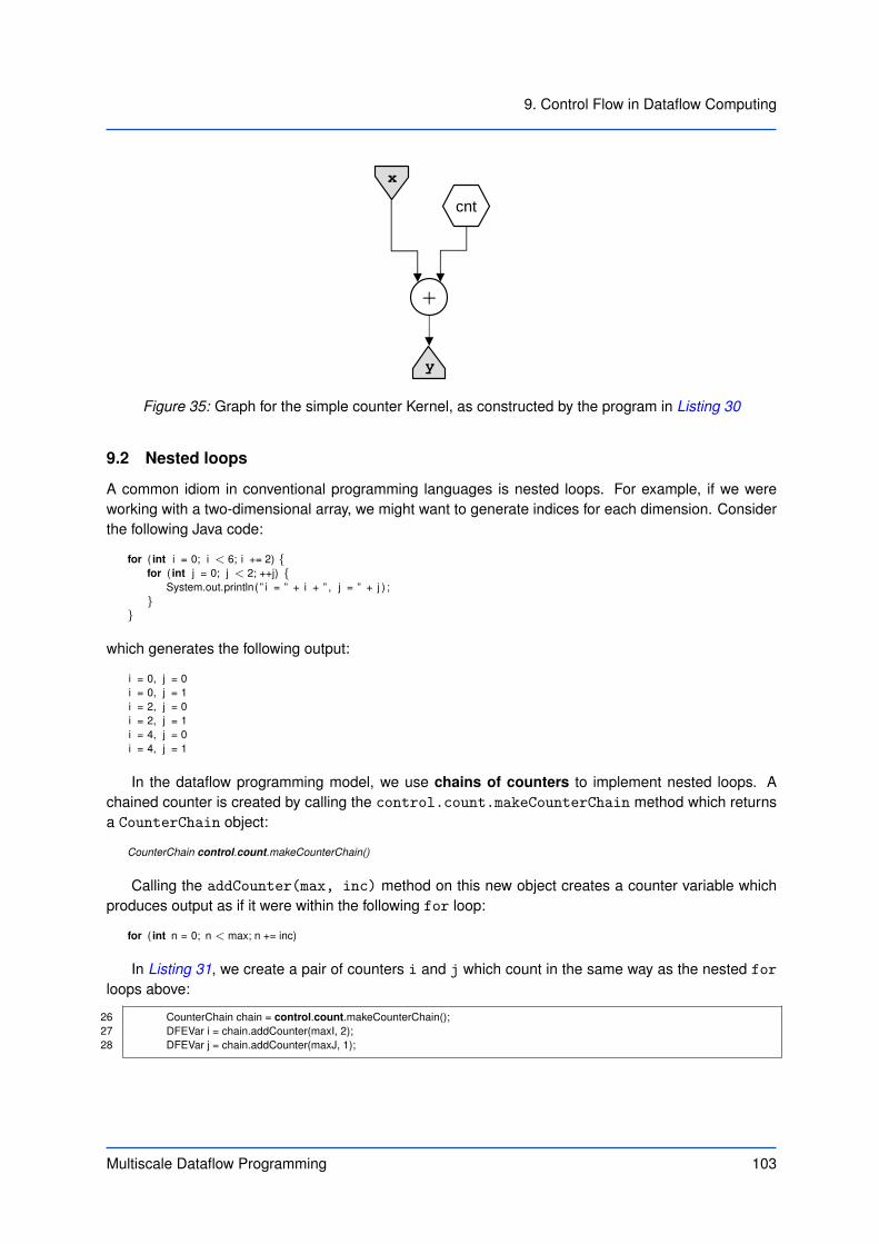
9. Control Flow in Dataflow Computing
cnt
y
+
x
Figure 35: Graph for the simple counter Kernel, as constructed by the program in Listing 30
9.2 Nested loops
A common idiom in conventional programming languages is nested loops. For example, if we wereworking with a two-dimensional array, we might want to generate indices for each dimension. Considerthe following Java code:
for ( int i = 0; i < 6; i += 2) {for ( int j = 0; j < 2; ++j) {
System.out.println( ” i = ” + i + ” , j = ” + j ) ;}
}
which generates the following output:
i = 0, j = 0i = 0, j = 1i = 2, j = 0i = 2, j = 1i = 4, j = 0i = 4, j = 1
In the dataflow programming model, we use chains of counters to implement nested loops. Achained counter is created by calling the control.count.makeCounterChain method which returnsa CounterChain object:
CounterChain control.count.makeCounterChain()
Calling the addCounter(max, inc) method on this new object creates a counter variable whichproduces output as if it were within the following for loop:
for ( int n = 0; n < max; n += inc)
In Listing 31, we create a pair of counters i and j which count in the same way as the nested for
loops above:
26 CounterChain chain = control.count.makeCounterChain();27 DFEVar i = chain.addCounter(maxI, 2);28 DFEVar j = chain.addCounter(maxJ, 1);
Multiscale Dataflow Programming 103

9.3 Advanced counters
Listing 31: A 2D counter Kernel using a counter chain (Simple2DCounterKernel.maxj).1 /∗∗2 ∗ Document: MaxCompiler Tutorial (maxcompiler-tutorial.pdf)3 ∗ Chapter: 9 Example: 2 Name: Simple two-dimensional counter4 ∗ MaxFile Name: Simple2DCounter5 ∗ Summary:6 ∗ Kernel that constructs a chained counter and outputs its7 ∗ values every cycle.8 ∗/9
10 package simple2dcounter;1112 import com.maxeler.maxcompiler.v2.kernelcompiler.Kernel;13 import com.maxeler.maxcompiler.v2.kernelcompiler.KernelParameters;14 import com.maxeler.maxcompiler.v2.kernelcompiler.stdlib.core.CounterChain;15 import com.maxeler.maxcompiler.v2.kernelcompiler.types.base.DFEVar;1617 class Simple2DCounterKernel extends Kernel {1819 Simple2DCounterKernel(KernelParameters parameters, int maxI, int maxJ) {20 super(parameters);2122 // Inputs23 DFEVar passThrough = io.input(”input”, dfeUInt(32));2425 // Create Counters26 CounterChain chain = control.count.makeCounterChain();27 DFEVar i = chain.addCounter(maxI, 2);28 DFEVar j = chain.addCounter(maxJ, 1);2930 i = i .cast(dfeUInt(32)) ;31 j = j .cast(dfeUInt(32)) ;3233 // Outputs34 io .output(” i ” , i , i .getType());35 io .output(” j ” , j , j .getType());36 io .output(”output” , passThrough, passThrough.getType());37 }38 }
9.3 Advanced counters
As a general control mechanism, a simpleCounter or CounterChain may not be flexible enough. It ispossible to create more complex counting behavior by specifying several characteristics of the counter:
bit width Counters generate a DFEUInt with the specified bit width. The bit width may be set to anynon-zero unsigned integer.
initial value By default a counter’s initial value is 0. The initial value parameter sets an arbitrarystarting point for counting.
increment The increment defaults to 1, and can be set to an arbitrary value via the increment param-eter. The increment parameter is combined with the count based on the ‘count mode’ below.
count mode There are three modes of counting:
• NUMERIC INCREMENTING — add an increment to the count on each enabled Kernel tick
• SHIFT LEFT — logically shift left the count on each enabled Kernel tick
104 Multiscale Dataflow Programming

9. Control Flow in Dataflow Computing
• SHIFT RIGHT — logically shift right the count on each enabled Kernel tick
The remainder of this document refers only to NUMERIC INCREMENTING counters, which is alsothe default counting mode.
maximum value By default, the maximum value of a counter is 2w − 1, where w is the bit width of thecounter. The maximum may also be set explicitly, in which case it must be an integer greater than0 which can be represented in w bits.
Additionally, it is possible to set the maximum value of the counter dynamically from anotherstream.
wrap mode What happens to a counter when it reaches its maximum is specified by the counter’s wrapmode. There are three wrap modes:
• COUNT LT MAX THEN WRAP — The counter counts up to and including max-1, then restartscounting from 0. For example, if the maximum is 5 and the increment is 1, the counter’svalues are:
0, 1, 2, 3, 4, 0, 1, 2, . . .
For a maximum value of 5 and an increment of 2 the values are:
0, 2, 4, 0, 2, 4, . . .
• STOP AT MAX — The counter stops at the greatest multiple of the increment not exceedingmaximum value until the Kernel is reset. This value is less than the maximum if the maxi-mum is not a multiple of the increment. For example, if the maximum is 5 and the incrementis 2 then the values are:
0, 2, 4, 4, 4, 4, . . .
• MODULO MAX OF COUNT — The counter’s value is calculated modulo the maximum value.For example, if the maximum is 5 and the increment is 2 then the count is:
0, 2, 4, 1, 3, 0, 2, 4, . . .
The default wrap mode is COUNT LT MAX THEN WRAP.
Whether or not a counter has wrapped can be found by getting the counter’s wrap signal. This isa Boolean state variable which is 1 during the last tick before wrapping. The wrap signal is oftenused when combining several counters together and is also useful as an input for watch nodes.
wrap value When a counter wraps, its next value is specified by the wrap value. By default this is 0.
enable The enable signal for a counter is a Boolean (one bit wide) DFEVar. For every tick where theenable is equal to 1, the counter counts and otherwise stays at the current value.
9.3.1 Creating an advanced counter
The parameters that specify an advanced counter’s behavior are encapsulated in a Count.Params
object which is returned by the count.makeParams method:
Count.Params control.count.makeParams(int bit width)
Multiscale Dataflow Programming 105

9.3 Advanced counters
The counter’s parameters can then be customized by calling the various with methods that are de-fined on Count.Params (e.g. withInc, withMax, etc.). These methods return a new Count.Params
object that can again be customized by subsequent calls to with methods.
W Note that Count.Params objects are immutable, so calling a with method does not modify theexisting object.
Once we have a suitable Count.Params object we can create a counter with the specified behaviorby calling the count.makeCounter method, using the Count.Params object as the only argument.This returns a Counter object:
Counter control.count.makeCounter(Count.Params params)
Once we have a Counter object we can get the counter’s value from the getCount method andthe ‘wrap’ signal by calling getWrap.
DFEVar getCount()DFEVar getWrap()
Listing 32 shows a Kernel design that creates an advanced counter. The corresponding Kernelgraph is shown in Figure 36.
We first make a Count.Params object with the specified bit width, maximum and increment:
31 Count.Params paramsOne = control.count.makeParams(width)32 .withMax(countOneMax)33 .withInc(countOneInc);
We use this Count.Params object to create our actual counter:
35 Counter counterOne = control.count.makeCounter(paramsOne);
We then create a second counter with the wrap signal of the first counter as its enable signal:
37 Count.Params paramsTwo = control.count.makeParams(width)38 .withEnable(counterOne.getWrap())39 .withMax(countTwoMax)40 .withWrapMode(WrapMode.STOP AT MAX);4142 Counter counterTwo = control.count.makeCounter(paramsTwo);
If we set count1Max to 3 and count2Max to 2, the two counters count as follows:ct1 = 0, 1, 2, 0, 1, 2, 0, 1, 2, 0, 1, 2, ...
ct2 = 0, 0, 0, 1, 1, 1, 2, 2, 2, 2, 2, 2, ...
106 Multiscale Dataflow Programming
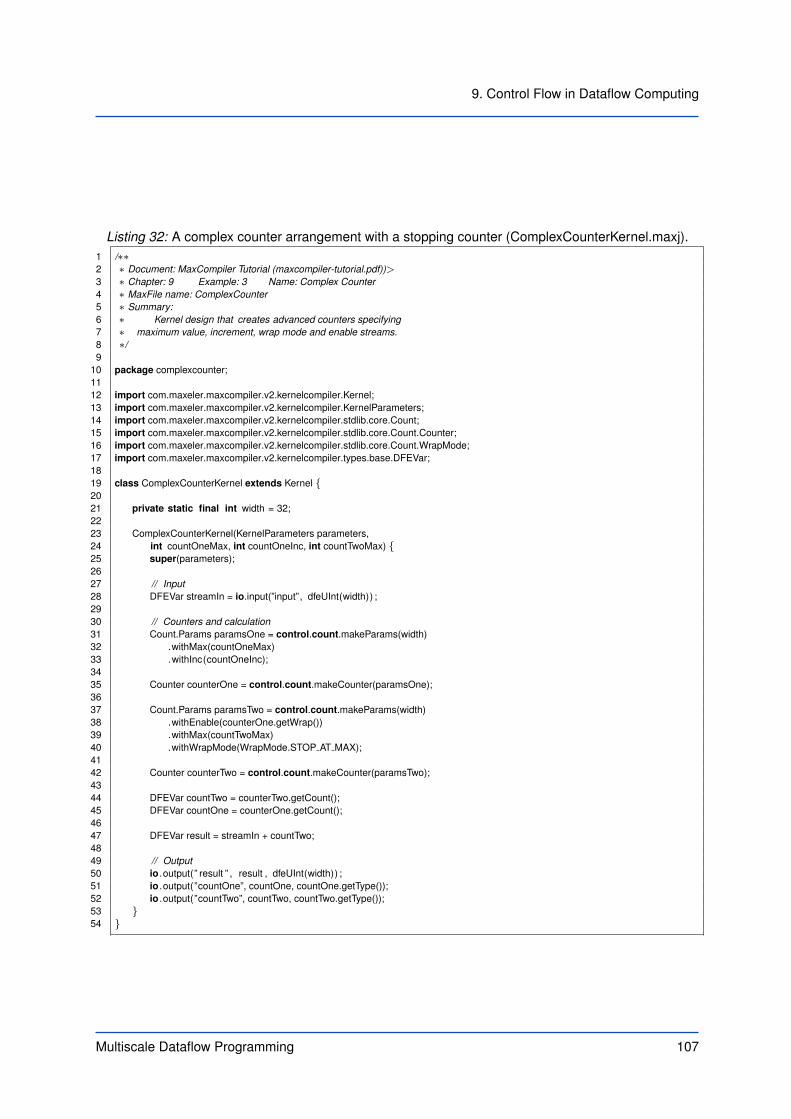
9. Control Flow in Dataflow Computing
Listing 32: A complex counter arrangement with a stopping counter (ComplexCounterKernel.maxj).1 /∗∗2 ∗ Document: MaxCompiler Tutorial (maxcompiler-tutorial.pdf))>3 ∗ Chapter: 9 Example: 3 Name: Complex Counter4 ∗ MaxFile name: ComplexCounter5 ∗ Summary:6 ∗ Kernel design that creates advanced counters specifying7 ∗ maximum value, increment, wrap mode and enable streams.8 ∗/9
10 package complexcounter;1112 import com.maxeler.maxcompiler.v2.kernelcompiler.Kernel;13 import com.maxeler.maxcompiler.v2.kernelcompiler.KernelParameters;14 import com.maxeler.maxcompiler.v2.kernelcompiler.stdlib.core.Count;15 import com.maxeler.maxcompiler.v2.kernelcompiler.stdlib.core.Count.Counter;16 import com.maxeler.maxcompiler.v2.kernelcompiler.stdlib.core.Count.WrapMode;17 import com.maxeler.maxcompiler.v2.kernelcompiler.types.base.DFEVar;1819 class ComplexCounterKernel extends Kernel {2021 private static final int width = 32;2223 ComplexCounterKernel(KernelParameters parameters,24 int countOneMax, int countOneInc, int countTwoMax) {25 super(parameters);2627 // Input28 DFEVar streamIn = io.input(”input”, dfeUInt(width)) ;2930 // Counters and calculation31 Count.Params paramsOne = control.count.makeParams(width)32 .withMax(countOneMax)33 .withInc(countOneInc);3435 Counter counterOne = control.count.makeCounter(paramsOne);3637 Count.Params paramsTwo = control.count.makeParams(width)38 .withEnable(counterOne.getWrap())39 .withMax(countTwoMax)40 .withWrapMode(WrapMode.STOP AT MAX);4142 Counter counterTwo = control.count.makeCounter(paramsTwo);4344 DFEVar countTwo = counterTwo.getCount();45 DFEVar countOne = counterOne.getCount();4647 DFEVar result = streamIn + countTwo;4849 // Output50 io .output(” result ” , result , dfeUInt(width)) ;51 io .output(”countOne”, countOne, countOne.getType());52 io .output(”countTwo”, countTwo, countTwo.getType());53 }54 }
Multiscale Dataflow Programming 107
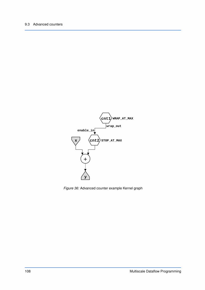
9.3 Advanced counters
Fig_Complex_Counter
y
+
x cnt2
cnt1
wrap_outenable_in
WRAP_AT_MAX
STOP_AT_MAX
Figure 36: Advanced counter example Kernel graph
108 Multiscale Dataflow Programming
9. Control Flow in Dataflow Computing
ExercisesExercise 1: Simple counter
Create a Kernel design that instantiates a simple counter. Derive from it a count that goes from 15down to zero, before wrapping from 15. Add this result to input stream x to produce output stream y.The CPU code is provided to test your implementation.
W Hint: you can use an algebraic expression of the output of a counter that goes from 0 up to 15.
Exercise 2: 2D counter
Make a 2D counter with the maximum values taken from scalar inputs. Set the scalar input for the fastdimension to 4 and for the slow dimension to 3. Test that the output of both counters is as expected.MaxCompiler requires that all Kernels have at least one input and one output: as the core has no input,add a dummy input that is connected directly to a dummy output. The number of dummy data valuessent to this core determines the number of values. Send in enough dummy data such that the counterin the slow dimension wraps.
Exercise 3: Advanced counter
This exercise revisits the 2D averaging filter with variable offsets from section 8. Adapt this exampleusing a 2D counter to keep track of the edges of each 2D array as it is streamed through the core. Applyboundary conditions to the edges, such that points that lie outside the 2D array do not contribute to theaverage. The average should be calculated based on the number of valid points, not simply divided by9 as before. CPU code is provided to stream in three consecutive 9x9 input arrays and verify that theoutput is as expected.
Multiscale Dataflow Programming 109

9.3 Advanced counters
110 Multiscale Dataflow Programming

10Advanced SLiC Interface
In section 2, we covered the Basic Static SLiC interface; in this section, we look at the Advanced Staticand Advanced Dynamic SLiC interfaces. We then look in more detail at SLiC engine interfaces, lookingthis time at how they are defined in the MaxCompiler source. We also see how to run dataflow enginesasynchronously using non-blocking functions, and cover the details of error handling, event monitoringand SLiC configuration. Finally we show how to use sliccompile to expose SLiC interfaces to scriptinglanguages.
To recap, the SLiC functions are split into three levels of increasing complexity and flexibility:
Basic Static allows a single function call to run the design on a single DFE using only static actionsdefined via a given function call interface.
Advanced Static allows control of loading of DFEs, setting multiple complex actions, and optimizationof CPU and DFE collaboration.
Advanced Dynamic allows for the full scope of dataflow optimizations and fine-grain control of alloca-tion and de-allocation of all dataflow resources.
10.1 The lifetime of a .max file
The life-cycle of a .max file within a CPU application is as follows:
Multiscale Dataflow Programming 111

10.2 Advanced Static
initialize - the .max file is initialized and functions become available.
load - the .max file is loaded onto a DFE. The DFE is now exclusively owned by the calling CPUprocess.
W Loading the .max file takes in the order of 100ms to 1s.
execute actions - the CPU calls SLiC functions to execute actions on the DFE.
W A loaded .max file has to be utilized for long enough to justify having waited up to asecond to load the configuration.
unload - the DFE is released by the CPU process and returns to the pool of DFEs managed by Max-elerOS.
free - the .max file is deallocated.
The Basic Static SLiC interface loads the .max file onto the DFE when the first SLiC function iscalled, and releases the DFE when the CPU process terminates. The Advanced Static SLiC interfaceallows you to control exactly when the DFE is loaded and unloaded.
10.2 Advanced Static
With the Advanced Static SLiC interface, the .max file must first be initialized using a method specificto the .max file. For our moving average example, this is:
max file t∗ MovingAverage init();
The .max file then gets loaded onto a DFE using max load:
max engine t∗ max load(max file t ∗max file, const char ∗engine id pattern);
engine id pattern is a string that indicates which engines to use. This takes the form
hostname[:engine_id],
with engine id either a number identifying a specific engine, or * for any engine. hostname canbe one of:
• The host name of an MPC-X node for remote engines
• "local" - for using local engines
• "*" - the host name is taken from the configuration variable "default engine resource"
112 Multiscale Dataflow Programming

10. Advanced SLiC Interface
The return value from max load is a handle for a DFE on which actions can be executed.
W The pattern format for arrays and groups of DFEs is different (see subsection 10.4 and subsec-tion 10.5).
10.2.1 Executing actions on DFEs
Actions are executed on a DFE using a structure containing the parameters for the action. This structureis specific to the .max file and engine interface. For example, for our moving average example, thedefault structure is:
typedef struct {int param N;const float ∗instream x;float ∗outstream y;
} MovingAverage actions t;
The populated action structure can be executed on the loaded DFE using the MovingAverage run
function:
void MovingAverage run(max engine t ∗engine,MovingAverage actions t ∗interface actions);
This function returns when the action is complete and the output data is available to the CPU code.Finally, once it is no longer needed, the DFE can be unloaded:
void max unload(max engine t ∗engine);
10.2.2 Holding the state of the DFE
The DFE can be loaded and unloaded multiple times during the execution of the CPU application torelease the DFE for use by other applications or to load an alternative .max file.
The state of the DFE is maintained between load and unloading. Once the DFE has been unloaded,there is no guarantee that the state, including the contents of the LMem, is maintained.
Let us examine an Advanced Static example. The CPU code below shows the moving averageCPU code required to run the .max file using the Advanced Static SLiC interface:
max file t ∗mavMaxFile = MovingAverage init();max engine t ∗mavDFE = max load(mavMaxFile, ”local:∗”);
MovingAverage actions t actions;actions.param N = size;actions.instream x = dataIn;actions.outstream y = dataOut;
MovingAverage run(mavDFE, &actions);
max unload(mavDFE);
Multiscale Dataflow Programming 113

10.3 Using multiple .max files
10.3 Using multiple .max files
Using the Advanced Static SLiC interface, two .max files can be loaded onto multiple DFEs or loadedsequentially on one DFE. This is achieved by including the header files for each .max file and callingthe appropriate functions for each file.
For example, imagine that we have our moving average .max file and another .max file calledThreshold.max that thresholds its input stream. Using the Advanced Static SLiC interface, we canrun the moving average, then reload the DFE with the thresholding .max file. passing the output of themoving average as the input:
#include ”MovingAverage.h”#include ”Threshold.h”#include <MaxSLiCInterface.h>
...max file t ∗mavMaxFile = MovingAverage init();max engine t ∗myDFE = max load(mavMaxFile, ”∗”);
MovingAverage actions t mavAction;mavAction.param N = size;mavAction.instream x = dataIn;mavAction.outstream y = mavOut;
MovingAverage run(myDFE, &mavAction);
max file t ∗threshMaxFile = Threshold init() ;max unload(myDFE);
myDFE = max load(threshMaxFile, ”∗”);Threshold actions t threshAction;threshAction.param N = size;threshAction.instream x = mavOut;threshAction.outstream y = dataOut;
Threshold run(myDFE, &threshAction);
max unload(myDFE);
10.4 Running .max files on multiple DFEs
A .max file can be run on multiple connected, adjacent DFEs with one command, using an arrayof actions in the Advanced Static and Advanced Dynamic SLiC interfaces. There are SLiC functionsspecific to the .max file with the array suffix for running such an array, for example:
void MovingAverage run array(max engarray t ∗engarray, MovingAverage actions t ∗interface actions[]);
There are also load and unload functions for arrays:
max engarray t∗ max load array(max file t ∗maxfile, int number of engines, const char ∗engine id pattern);
void max unload array(max engarray t ∗engarray);
The engine id pattern argument for arrays is one of:
• The host name of an MPC-X node when using remote engines
• "local" - use local engines;
• "*" - the host name is taken from the configuration variable "default engine resource".
114 Multiscale Dataflow Programming

10. Advanced SLiC Interface
The array of actions is specified as a C array of pointers to action structures, as shown in thefollowing example, which runs our moving average .max file on two DFEs:
const int numEngines = 2;MovingAverage actions t ∗actions[numEngines];
for ( int i = 0; i < numEngines; i++) {actions[ i ] = malloc(sizeof(MovingAverage actions t));actions[ i ]−>param N = size;actions[ i ]−>instream x = dataIn[i];actions[ i ]−>outstream y = dataOut[i];
}
max file t ∗maxfile = MovingAverage init();max engarray t ∗engines = max load array(maxfile, numEngines, ”∗”);Maxring run array(engines, actions);
max unload array(engines);max file free (maxfile) ;
The DFEs in an array may communicate with each other via MaxRing connections. MaxRing iscovered in more detail in section 13.
10.5 Sharing DFEs
Engine groups are multiple DFEs loaded with the same .max file, shared between threads, processesand users. Engine groups can optionally gain or lose real engines over time: this is managed byMaxelerOS at runtime.
An engine group is created using max load group:
max group t∗ max load group(max file t ∗max file,max sharing mode t sharing mode,const char ∗group id,int group size);
sharing mode specifies how to share the DFEs and must be one of:
• MAXOS EXCLUSIVE indicates that no other process can use an engine that belongs to the group:this is also the behavior when not using groups.
• MAXOS SHARED is used for fine-grained sharing between processes, where no .max file loadingtakes place except on creating the group.
• MAXOS SHARED DYNAMIC allows the system to re-size the group and load/unload engines withoutexplicit instruction from the user.
Table 5 summarizes the sharing and group size behavior for each of the sharing modes.group id is of the form grouptag [@ hostname], where hostname is one of:
• The host name of an MPC-X node when using remote engines
• "local" - use local engines
• "*" - the host name is taken from the configuration variable "default engine resource"
In cases where @ is absent, the entire string is used as the group tag. group size is the requirednumber of DFEs in the group, or the initial number for a DYNAMIC group.
Multiscale Dataflow Programming 115

10.5 Sharing DFEs
Sharing mode Share engines between processes1 Group size changed by user or system
MAXOS EXCLUSIVE no noMAXOS SHARED yes2 noMAXOS SHARED DYNAMIC yes2 yes
1 Engines can always be shared between threads in the same process.2 Only processes with the same group ID can share engines in a group.
Table 5: Group properties.
10.5.1 Running actions on a DFE in a group
For individual engines and arrays, once they are loaded they are also locked for exclusive use, whereaswith groups an additional lock step is required. An available DFE from the group is locked for use bycalling max lock any:
max engine t∗ max lock any(max group t ∗group);
This function returns as soon as an engine becomes available. Once an engine has been locked,actions are executed on it using the SLiC functions specific to the .max file.
The max unlock function releases the DFE back to the group:
void max unlock(max engine t ∗engine);
Finally, the group can be unloaded when it is no longer required using max unload group:
void max unload group(max group t ∗group);
We can take our moving average as an example again. This time, we load the .max file to a groupand run it on a DFE from the group:
max file t ∗mavMaxFile = MovingAverage init();
max group t ∗mavGroup = max load group(mavMaxFile, MAXOS EXCLUSIVE, ”mavGroup@local:∗”, 2);
MovingAverage actions t actions;actions.param N = size;actions.instream x = dataIn;actions.outstream y = dataOut;
max engine t ∗mavDFE = max lock any(mavGroup);
MovingAverage run(mavDFE, &actions);max unlock(mavDFE);
max unload group(mavGroup);
If you only need to execute a single action on an engine, it is possible to use a high-performanceatomic execution directly on the engine group. This will queue and execute the actions on any engine inthe group then return. This type of interface is particularly useful when large numbers of CPU threadsare submitting many small jobs on many engines. To use, use the auto-generated function:
MovingAverage run group(max group t ∗group, MovingAverage actions t ∗interface actions);
This replaces the uses of max lock any, MovingAverage run and max unlock in the previousexample.
116 Multiscale Dataflow Programming

10. Advanced SLiC Interface
Property On max load At other timesMAXOS EXCLUSIVE Always, unless there is already
a free engine with the same.max file loaded
Never
MAXOS SHARED Always, unless there is alreadya free engine with the same.max file loaded, which mayhave been loaded by anotherprocess 1
NeverMAXOS SHARED DYNAMIC If the user software requests to
resize the group, or the systemresizes the group based on de-mand
1 Other processes can lock the engine after it has been loaded in one process.
Table 6: Engine loading behavior for different group properties.
10.5.2 Engine loads
MaxelerOS manages the loading of the .max file onto a DFE when required. When the .max file isloaded depends on the sharing mode and is detailed in Table 6.
10.6 Advanced Dynamic
The Advanced Dynamic SLiC interface offers all of functionality of the Advanced Static, but using stringsto specify the parameters to functions to use a .max file, rather than static functions and structuresdefined in the .max file. This allows Advanced Dynamic CPU code to be decoupled from a particular.max file.
.max file initialization, engine loading and engine loading are performed in the same way as theAdvanced Static (see subsection 10.2).
Actions are defined using a max actions t structure, which is initialized using max actions init:
max actions t ∗max actions init( max file t ∗max file, const char ∗interface);
The max file argument is a pointer to the initialized .max file handle and interface is the engineinterface to use. Using NULL as the interface argument specifies that no engine interface is to beused.
A function API is used to configure the actions max actions t structure.
10.6.1 Setting engine interface parameters
Engine interface parameters can be set using max set param uint64t for integer values, ormax set param double for floating-point values:
void max set param uint64t(max actions t∗ actions, const char ∗ const name, uint64 t value);void max set param double(max actions t∗ actions, const char ∗ const name, double value);
The name argument is the string name for the engine interface parameter as defined in the Manager.
Multiscale Dataflow Programming 117

10.6 Advanced Dynamic
Likewise, there are functions for setting each element for arrays of engine interface parameters,max set param array uint64t and max set param array double:
void max set param array uint64t(max actions t ∗actions, const char ∗ const name, uint64 t value, int idx) ;void max set param array double(max actions t ∗actions, const char ∗ const name, double value, int idx);
Calling the functions to set engine interface parameters when the max actions t has been initial-ized without an engine interface (i.e. set to NULL) is invalid and raises an error:
SLiC Error #517 @ actions_interfaces_internal.c:39 - Interface parameter "N"
cannot be set for engine interface "(null)"
SLiC Error #518 @ actions.c:77 - Error reported from function "
max_set_param_uint64t".
10.6.2 Streaming data
Data is added to input and output streams for an action set using max queue input andmax queue output:
void max queue input(max actions t ∗actions, const char ∗stream name, const void ∗data, size t bytes);void max queue output(max actions t ∗actions, const char ∗stream name, const void ∗data, size t bytes);
The bytes argument is the number of bytes of input data or the size of the memory allocated forthe output data.
One advantage of the max queue interface is that it can be called multiple times as part of a singleactions object to queue multiple data transfers back-to-back. This can be used to ”gather“ data frommemory into the DFE, ”scatter“ results into CPU memory, or to stream the same input data multipletimes (by passing the same input pointer). Passing the same data pointer multiple times to an outputstream leads to only the last values written to the memory being available.
10.6.3 Freeing the action set
When an action set is no longer needed, the memory can be released using max actions free:
void max actions free(max actions t ∗actions);
W Failing to free an action set when it is no longer needed can lead to memory leaks.
10.6.4 Advanced Dynamic example
The code below shows the moving average example again, this time using the Advanced Dynamic SLiCinterface:
max file t ∗mavMaxFile = MovingAverageSimple init();max engine t ∗mavDFE = max load(mavMaxFile, ”local:∗”);
max actions t ∗actions = max actions init (mavMaxFile, ”default”);max set param uint64t(actions, ”N”, size) ;max queue input(actions, ”x”, dataIn, sizeBytes);max queue output(actions, ”y”, dataOut, sizeBytes);
118 Multiscale Dataflow Programming

10. Advanced SLiC Interface
max run(mavDFE, actions);
max actions free(actions);
max unload(mavDFE);
10.6.5 Setting and retrieving Kernel settings
The number of Kernel ticks for a Kernel to run for is set using max set ticks with the name of theKernel:
void max set ticks(max actions t ∗actions, const char ∗kernel name, uint64 t nb ticks);
Stream offsets are set using max set offset with the name of the Kernel and the name of theoffset:
void max set offset(max actions t∗actions, const char∗kernel name, const char∗offset var name, int v);
Stream distance measurements and autoloop sizes (see Acceleration Tutorial - Loops and Pipelin-ing) can be retrieved from a Kernel:
int max get stream distance(max actions t ∗actions, const char ∗kernel name, const char ∗offset var name);int max get offset auto loop size(max actions t ∗actions, const char ∗kernel name, const char ∗offset var name);
10.6.6 Setting and reading mapped memories
Elements of mapped memories on a Manager block or Kernel are set individually usingmax set mem uint64t or max set mem double, depending on the type contained in the memory:
void max set mem uint64t(max actions t ∗actions, const char ∗block name, const char ∗mem name, size t index, uint64 t v);void max set mem double(max actions t ∗actions, const char ∗block name, const char ∗mem name, size t index, double v);
Validation checks whether all of the elements in a mapped memory have been set.Likewise, pointers for reading back each mapped memory element are set using
max get mem uint64t or max get mem double:
void max get mem uint64t(max actions t ∗actions, const char ∗block name, const char ∗mem name, size t index, uint64 t ∗v);void max get mem double(max actions t ∗actions, const char ∗block name, const char ∗mem name, size t index, double ∗v);
10.6.7 Action validation
The Advanced Dynamic SLiC interface provides automatic checking of actions before they are run ona DFE, ensuring that all the required parameters have been set correctly.
If we were to make a mistake in the CPU code for our moving average example, perhaps forgettingto set the size engine interface parameter for the default engine interface, the validation of the actionswhen they are run on the engine would raise an error:
Tue 17:10: SLiC Error #517 @ actions_interfaces_internal.c:182 - Interface
parameter "N" not defined for engine interface "default"
Tue 17:10: SLiC Error #518 @ maxfile_setup.c:486 - Error reported from
function "max_actions_get_param_uint64t".
Tue 17:10: Aborted
Multiscale Dataflow Programming 119

10.7 Engine interfaces
There are functions in the API to tell SLiC to ignore specific parameters for a set of actions whenperforming this checking:
void max ignore route(max actions t ∗actions, const char ∗block name);void max ignore offset( max actions t ∗actions, const char ∗kernel name, const char ∗offset var name);void max ignore kernel(max actions t ∗actions, const char ∗kernel name);void max ignore block(max actions t ∗actions, const char ∗block name);
For a mapped memory, the whole memory can be ignored, or just the input or output:
void max ignore mem(max actions t ∗actions, const char ∗block name, const char ∗mem name);void max ignore mem input(max actions t ∗actions, const char ∗block name, const char ∗mem name);void max ignore mem output(max actions t ∗actions, const char ∗block name, const char ∗mem name);
Validation for a set of actions can be disabled altogether:
void max disable validation(max actions t ∗actions);
W Disabling action validation makes it possible to execute an incomplete set of actions, which canlead to bugs that are hard to track down.
10.6.8 Groups and arrays of engines
Groups and arrays of engines behave in the same way as when using the Advanced Static level func-tions (see subsection 10.4 and subsection 10.5).
In the case of arrays, there is an Advanced Dynamic function for running the array, max run array:
void max run array(max engarray t ∗engarray, max actarray t ∗actarray);
For groups of engines, when no state needs to be maintained between operations on a DFE,max run group locks, runs and unlocks the DFE via a single function call:
void max run group( max group t ∗group, max actions t ∗actions);
10.7 Engine interfaces
Engine interfaces encapsulate different behavior or stages of execution for a .max file, simplifying theAPI for the CPU programmer. You can control which parameters and I/O are available in each engineinterface, with inputs and outputs for the .max file either ignored or set automatically based on inputsfrom the CPU code.
Engine interfaces can be used to control the APIs for all inputs and outputs to the .max file.
• Number of ticks for Kernels to run
• Streams between the CPU and the DFE
• Streams to or from the LMem (see section 13)
• Scalar inputs and outputs
• Mapped memory inputs and outputs
120 Multiscale Dataflow Programming

10. Advanced SLiC Interface
• Offset parameters
• Routing blocks (fanout, multiplexers and demultiplexers) in Custom Managers (see ManagerCompiler Tutorial)
• Autoloop offset values (see Acceleration Tutorial - Loops and Pipelining)
• Kernel distance measurements (see Acceleration Tutorial - Loops and Pipelining)
In the default engine interface, an argument for the number of ticks is added to the SLiC inter-face, and all streams are assumed to contain a number of elements equal to that number of ticks. Allscalar inputs and outputs, mapped memories, stream offset parameters and Manager routing blocksare automatically added to the SLiC Interface, unless the default engine interface is overridden (seesubsubsection 10.7.2). The only exceptions are AutoLoop offset values and Kernel distance measure-ments, which must be added explicitly (see subsubsection 10.8.3).
10.7.1 Adding an engine interface to a Manager
A standard simple engine interface is added to a .max file when createSLiCinterface is calledwithout any arguments. This type of interface works for many simple programs but may not be flexibleenough for all of your dataflow programs.
For complicated managers and kernels, custom engine interfaces can be added by creating aninstance of the EngineInterface class, configuring the settings for the engine interface and thencalling createSLiCinterface with the engine interface as a parameter, for example:
...Manager manager = new Manager(params);...EngineInterface myInterface = new EngineInterface(”myInterface”);...manager.createSLiCinterface(myInterface);manager.build();...
Instances of EngineInterface are declared with a string for the name and an optional stringargument doc for text that appears in the comments in the .max file and SLiC header file:
public EngineInterface(String name, String doc)public EngineInterface(String name)
10.7.2 The default engine interface
Engine interfaces are given names by the MaxJ programmer, resulting in a interface to the Maxfilenamed maxfilename interfacename. If the engine interface is given the special name “default” (orthe shortcut constructor EngineInterface() is used), then the resulting function gets the specialname maxfilename only. This is particularly suitable for DFEs which have one primary interface butmay have other supporting interfaces to be used to perform specific operations.
If you do not create a “default” engine interface yourself, an interface will automatically be createdwhich exposes all parameters for the kernels and manager.
For some DFEs, a “default” engine interface is inappropriate, so you can completely suppress thedefault engine interface from the SLiC API using the suppressDefaultInterface method on theManager class.
Multiscale Dataflow Programming 121

10.7 Engine interfaces
10.7.3 Ignoring unset parameters
It is common for a .max file not to require a particular parameter to be set or visible for a given engineinterface. All parameters that are not explicitly set in a engine interface can be ignored using theignoreAll method:
void ignoreAll ( Direction flag )
122 Multiscale Dataflow Programming

10. Advanced SLiC Interface
The flag argument selects whether to ignore only inputs, outputs or both:
public static enum Direction {IN,OUT,IN OUT;
};
Direction.IN refers to all settings that are sent from the CPU to the DFE, and includes:
• Number of ticks for Kernels to run
• Stream inputs from the CPU to the DFE
• Stream outputs from the DFE to the CPU
• Streams to or from the LMem
• Scalar inputs
• Mapped memory inputs
• Offset parameters
• Routing blocks (fanout, multiplexers and demultiplexers) in Custom Managers (see ManagerCompiler Tutorial)
Direction.OUT refers to data that is returned from the .max file or DFE to the CPU application:
• Scalar outputs
• Mapped memory outputs
• Autoloop offset values (see Acceleration Tutorial - Loops and Pipelining)
• Kernel distance measurements (see Acceleration Tutorial - Loops and Pipelining)
10.7.4 Ignoring specific parameters
Individual parameters can be suppressed in the API using one of a set of ignore methods on theengine interface:
void ignoreLMem(String streamName)void ignoreStream(String streamName)void ignoreRoute(String routingBlock)
void ignoreOffset(String blockName, String offsetName)void ignoreScalar(String blockName, String scalarName)
In the case of mapped memories, whether to ignore inputs, outputs or both must also be specified,again using the Direction enum:
void ignoreMem(String blockName, String memName, Direction flag)
Similarly, parameters can be unignored:
void unignoreScalar(String blockName, String scalarName)void unignoreMem(String blockName, String memName)void unignoreDistanceMeasurement(String kernelName, String name)void unignoreAutoLoopOffset(String kernelName, String name)
Multiscale Dataflow Programming 123

10.8 Engine interface parameters
Unignoring parameters is useful when used in conjunction with a call to ignoreAll to simplify thecode where there is a large number of parameters.
10.7.5 Ignoring an entire Kernel
All of the inputs and outputs for a particular Kernel can be ignored with a single method call:
void ignoreKernel(String kernelName)
10.8 Engine interface parameters
An engine interface parameter is a user-defined parameter that can be used to express relationshipsbetween kernel entities such as tick count and stream length. Simple arithmetic operations may beperformed with engine interface parameters to make more complex relationships.
Engine interface parameters can be created using the addParam method, which has two variants,the second of which takes a string argument doc to add documentation for the end-user of the .max
file.
InterfaceParam addParam(String name, CPUTypes type)InterfaceParam addParam(String name, CPUTypes type, String doc)
An engine interface parameter becomes an input argument in the SLiC API with the specified CPUtype. type can be any of the following values:
public enum CPUTypes {UINT8, // -> uint8 tINT8, // -> int8 tUINT16, // -> uint16 tINT16, // -> int16 tINT, // -> int ( int64 t )INT32, // -> uint32 tUINT32, // -> uint32 tUINT64, // -> uint64 tINT64, // -> int64 tFLOAT,DOUBLE,VOID;}
For example, consider adding an engine interface parameter for the size of the incoming datastream:
...EngineInterface myInterface = new EngineInterface();InterfaceParam inputDataSize = myInterface.addParam(”inputDataSize”, UINT32, ”The size of the input data stream in words”);...
124 Multiscale Dataflow Programming

10. Advanced SLiC Interface
This appears as a 32-bit, unsigned integer argument in the Basic Static SLiC interface:
/∗∗∗ \brief Simple static function for the engine interface ’ default ’.∗∗ ...∗ \param [in] param inputDataSize Interface Parameter ”inputDataSize”: The size of the input data stream in words∗ ...∗/
void MyMaxFile(...int32 t param inputDataSize,...) ;
10.8.1 Kernel settings
Various Kernel configuration options can be set in a SLiC engine interface:
• Number of ticks for Kernels to run
void setTicks(String blockName, InterfaceParam p)void setTicks(String blockName, long p)
• Stream settings
void setStream(String streamName, CPUTypes type, InterfaceParam p)void setStream(String streamName, CPUTypes type, long p)
• Mapped memory inputs
void setMem(String blockName, String memoryName, int index, double value)void setMem(String blockName, String memoryName, int index, long value)void setMem(String blockName, String memoryName, int index, InterfaceParam value)
• Offset expressions
void setOffset(String blockName, String offsetName, InterfaceParam p)void setOffset(String blockName, String offsetName, long p)
• Scalar inputs
void setScalar(String blockName, String scalarName, long value)void setScalar(String blockName, String scalarName, double value)void setScalar(String blockName, String scalarName, InterfaceParam p)
In each case, overloaded versions of the methods allow the values to be set either from a Javavariable or from an engine interface parameter.
There are no explicit functions for retrieving the values of scalar outputs or mapped-memory out-puts: these are automatically added by the engine interface, unless disabled using ignoreScalar orignoreMem, as described in subsubsection 10.7.4.
Multiscale Dataflow Programming 125

10.8 Engine interface parameters
10.8.2 LMem settings
LMem settings can be set either using all Java variables or all engine interface parameters:
void setLMemLinear(String streamName, long address, long size)void setLMemLinear(String streamName, InterfaceParam address, InterfaceParam size) {
void setLMemLinearWrapped(String streamName, InterfaceParam address, InterfaceParam arrSize, InterfaceParam rwSize,InterfaceParam offset)
void setLMemLinearWrapped(String streamName, long address, long arrSize, long rwSize, long offset) {
void setLMemStrided(String streamName, long address, long sizeFast, long sizeSlow, long strideMode)void setLMemStrided(String streamName, InterfaceParam address, InterfaceParam sizeFast, InterfaceParam sizeSlow,
InterfaceParam strideMode)
void setLMemBlocked(String streamName, long address,long arraySizeFast, long arraySizeMed, long arraySizeSlow,long rwSizeFast, long rwSizeMed, long rwSizeSlow,long offsetFast, long offsetMed, long offsetSlow )
void setLMemBlocked(String streamName, InterfaceParam address,InterfaceParam arraySizeFast, InterfaceParam arraySizeMed, InterfaceParam arraySizeSlow,InterfaceParam rwSizeFast, InterfaceParam rwSizeMed, InterfaceParam rwSizeSlow,InterfaceParam offsetFast, InterfaceParam offsetMed, InterfaceParam offsetSlow )
void setLMemInterruptOn(String streamName)
Two methods are provided to create an engine interface parameter instance from a Java variable:
InterfaceParam addConstant(double value)InterfaceParam addConstant(long value)
For details on LMem access patterns and interpretation of the settings, see subsection 13.3.
10.8.3 Autoloop offset parameters and distance measurements
Engine interface parameters to retrieve autoloop offset parameters and distance measurements (seethe Loops and Pipelining Acceleration Tutorial) from a Kernel can be added to an engine interface:
InterfaceParam getAutoLoopOffset(String kernelName, String name)InterfaceParam getDistanceMeasurement(String kernelName, String name)
These parameters are special cases that are added to the SLiC API as outputs to the CPU code,as well as behaving as standard InterfaceParam objects for the purposes of setting parameters onKernels or Managers. For example, let us take adding a distance measurement in an engine interface:
EngineInterface myInterface = new EngineInterface();InterfaceParam loopLength = myInterface.getDistanceMeasurement(”myKernel”, ”loopLength”);
This adds an argument param MyKernel loopLength to the SLiC interface, for example in thecase of Basic Static:
void MyMaxFile(...int32 t ∗param MyKernel loopLength,...) ;
126 Multiscale Dataflow Programming

10. Advanced SLiC Interface
If the engine interface parameter for an autoloop offset parameter or distance measurement is onlyused in the Manager itself, for example in a calculation to set a Kernel or Manager parameter, it can besuppressed from the SLiC interface:
void ignoreAutoLoopOffset(String kernelName, String name)void ignoreDistanceMeasurement(String kernelName, String name)
10.8.4 Engine interface parameter arrays
Engine interface parameter arrays allow an array of data to be passed from the CPU code to the .max
file:
public InterfaceParamArray addParamArray( String name, CPUTypes type, String doc )public InterfaceParamArray addParamArray( String name, CPUTypes type )
Within a Manager, the InterfaceParam elements of the array are accessed using the array access[] operator, using either a InterfaceParam or a Java integer as the index.
In many cases, the size of the engine interface parameter array can be inferred from the engineinterface code, for example:
InterfaceParamArray coeff = myInterface.addParamArray(”coeff”, CPUTypes.FLOAT);for ( int i = 0 ; i < 100 ; i++ ) {
myInterface.setScalar(”myKernel”, ” filter ” + i , coeff [ i ]) ;}
This may not be possible if the engine interface parameter array is indexed only using by anInterfaceParam instance, for example:
InterfaceParam idx = myInterface.addParam(”idx”, CPUTypes.UINT32);InterfaceParamArray coeff = myInterface.addParamArray( ”coeff”, CPUTypes.FLOAT);myInterface.setScalar(”myKernel”, ”myScalar”, coeff[ idx ] ) ;
In this case, the size of the engine interface parameter array must be set explicitly:
coeff .setMaxSize( 100 );
10.9 .max file constants
In many designs, a .max file is built with a number of compile-time parameters that define, for example,behavior, limits or dimensions. These can be passed to the CPU code as constants in the .max file.
Three methods on the Manager class are provided for defining integer, floating-point and stringconstants that appear as #defines in the SLiC header file:
void addMaxFileConstant(String name, int value)void addMaxFileStringConstant(String name, String value)void addMaxFileDoubleConstant(String name, double value)
The name argument is the string that is appended to the name of the .max file to give the nameof the constant in the SLiC header file, for example, for a .max file with the name MyMaxfile and afloating-point constant myconstant with the value 0.5, the resultant #define appears as:
1 #define MyMaxfile myconstant (0.5)
Multiscale Dataflow Programming 127
10.10 Asynchronous execution
It is also possible to retrieve maxfile constants using dynamic functions, namedmax get constant string, max get constant double and max get constant uint64t, de-pending on the type of the constant.
10.10 Asynchronous execution
In many applications, it is more efficient for the CPU application to continue executing code while theDFE is running a set of actions. SLiC provides non-blocking versions of the functions we have seenso far for running actions on engines, groups and arrays. These functions return immediately once theactions have been committed, allowing the CPU application to continue execution.
Initialization, loading and unloading of .max files onto DFEs is performed in the same way as forthe blocking API functions. When it comes to running individual DFEs, arrays or groups of DFEs, thereare nonblock versions of the Static SLiC Interface functions in the .max file header file. For example,our moving average has the following non-blocking functions:
max run t ∗MovingAverage nonblock(int32 t param N, const float ∗instream x, float ∗outstream y);max run t ∗MovingAverage run nonblock(max engine t ∗engine, MovingAverage actions t ∗interface actions);max run t ∗MovingAverage run group nonblock(max group t ∗group, MovingAverage actions t ∗interface actions);max run t ∗MovingAverage run array nonblock(max engarray t ∗engarray, MovingAverage actions t ∗interface actions[]);
Likewise, there are Advanced Dynamic non-blocking functions:
max run t∗ max run nonblock(max engine t ∗engine, max actions t ∗actions);max run t∗ max run array nonblock(max engarray t ∗engarray, max actarray t ∗actarray);max run t∗ max run group nonblock(max group t ∗group, max actions t ∗actions);
All of these non-blocking functions return a handle to the execution status (a pointer to a max run t
structure), or NULL in the case of an error. To re-synchronize with the DFE, there is a function to waitfor the actions to complete for an execution handle:
void max wait(max run t ∗run);
In the case of arrays of DFEs, this waits for the set of actions to be completed on all the DFEs inthe array.
Calling a non-blocking run function on the same DFE(s) queues up action sets: this helps minimizeany idle time between actions on a DFE, especially when running remote DFEs on an MPC-X node.
To indicate to SLiC that the outcome of a set of actions being executed is to be ignored in the CPUcode, max nowait must be called:
void max nowait(max run t ∗run);
This can be useful when queuing a number of action sets on a DFE (or array of DFEs), so that theCPU application only need wait for the last one to be completed.
W Either max wait or max nowait must be called for every execution status handle to ensurethat SLiC can release all the associated memory.
128 Multiscale Dataflow Programming

10. Advanced SLiC Interface
Wmax nowait cannot be run on an execution status handle for actions running on a group ofDFEs, as actions may be executed out of sequence. Calling max nowait with such a handleraises an error.
10.10.1 Asynchronous execution example
The moving average from section 3 can be modified to run the CPU version of the moving average atthe same time as the moving average is being executed on the DFE:
max run t ∗execStatus = MovingAverage nonblock(size, dataIn, dataOut);
MovingAverageCPU(size, dataIn, expected);
/∗ Other CPU work can be done here. ∗/
max wait(execStatus);
And using the Advanced Static API:
max file t ∗mavMaxFile = MovingAverage init();max engine t ∗mavDFE = max load(mavMaxFile, ”local:∗”);
MovingAverage actions t actions;actions.param N = size;actions.instream x = dataIn;actions.outstream y = dataOut;
max run t ∗execStatus = MovingAverage run nonblock(mavDFE, &actions);
MovingAverageCPU(size, dataIn, expected);
/∗ Other CPU work can be done here. ∗/
max wait(execStatus);
max unload(mavDFE);
10.11 Error handling
Errors are reported into error contexts, which are instances of the max errors t structure. There area number of handles in SLiC that contain an error context:
max file t - .max file handles
max actions t - action sets
max engine t - engine handles
max engarray t - engine array handles
max actarray t - action set array handles
max group t - engine group handles
max run t - execution status handle (see subsection 10.10)
Multiscale Dataflow Programming 129

10.11 Error handling
The error context is called errors in every case and thus can be accessed as, for examplemymaxfile->errors.
By default, SLiC is configured to abort execution of the CPU program on an error. This can bedisabled using max errors mode:
void max errors mode(max errors t ∗errors, int abort on error);
A value for abort on error of 0 instructs the application not to abort for the specified error context,1 instructs it to abort.
Setting max errors mode on an error context for a handle sets the error contexts for all the handlescreated from it to have the same behavior. For example, setting the error context for a .max file to notabort on an error causes all arrays, groups, engines, actions and action arrays created from the .max
file handle to also not abort on an error. Where a function takes multiple handles as arguments, theabort behavior of the returned handle is inherited from the engine, array or group handle. Individualerror contexts that have inherited abort behavior can still be changed if required.
max ok is used to check an error context on a handle once a function has returned:
int max ok(max errors t ∗errors);
This returns 1 if there are no errors or 0 if there are errors. Alternatively specific errors can bechecked using max errors check:
int max errors check(max errors t ∗ errors, int error code);
This takes an integer argument for the error code and returns 1 if the error has been raised or 0 ifnot.
W For error contexts that are not set to abort on error, the error context of every handle passedas an argument to a function must be checked once that function has returned.
W For error contexts that are not set to abort on error, handles returned from SLiC functions mustalways be tested for NULL.
A text trace of the error can be retrieved by passing the error context to max errors trace:
char∗ max errors trace(max errors t ∗ errors);
The returned string is allocated by the function and must be deallocated as appropriate by yourCPU application.
130 Multiscale Dataflow Programming

10. Advanced SLiC Interface
Option string Type Default Description
default pcie timeout integer 30 Default timeout for PCIE stream trans-fer (seconds)
default wfi timeout integer 30 Default timeout for interrupt wait (sec-onds)
default topology timeout integer -1 (infinite) Default timeout for topology allocation(seconds)
default maxdebug mode enum never Default debug mode, see Figure 5.3.5verbose Boolean false Enable full debug outputeventlog ignore errors Boolean false Ignore errors in the event logging mod-
uleeventlog enable Boolean false Enable event monitoring, even if it is
not enabled in the CPU codedfeprintf enable Boolean true Enable dfePrintf outputfind next debug dir Boolean true Change the debug directory name if
the current one already existsprintf to stdout Boolean true Stream Debug.printf to standard
outputdefault engine resource string NULL Default location of the enginesuse simulation string NULL Simulation server socketdefault eventlog server string NULL Name of event logging serverdefault eventlog process name string NULL Event logging process namedebug dir string debug Directory where debug output is writ-
ten
Table 7: SLiC configuration options.
10.12 SLiC configuration
In addition to the configuration available through the C interface, aspects of SLiC can be configuredthrough both configuration files and environment settings. The inputs are parsed in this order:
1. File defined in environment variable $SLIC DEFAULT CONF FILE
2. File ~/.MaxCompiler slic user.conf
3. File defined in environment variable $SLIC CONF FILE
4. Settings defined in environment variable $SLIC CONF (used by MaxIDE and example Makefiles)
There are integer, Boolean and string settings, shown with their default values and description inTable 7. Settings are defined as key-value pairs of the form option=value. In a configuration file, onepair is defined per line, for example:
#set timeouts
default_pcie_timeout = 60
default_wfi_timeout = 60
In the environment variable, pairs are separated by the ; character, for example:
Multiscale Dataflow Programming 131

10.13 Debug directories
export SLIC_CONF="default_pcie_timeout = 60;default_wfi_timeout = 60"
Comments can be added to the file by beginning a line with the # character. Empty lines are ignored.
10.13 Debug directories
A SLiC application may produce a number of debug output files, as covered in section 5:
• when the application is run from within MaxIDE, these output files are generated in a time-stamped directory present under the debug in the corresponding RunRule folder, e.g.RunRules/Simulation/debug/2013.07.03-14.16.30-380-BST;
• when the application is run from the command line, these outputs are generated in a directorybelow the current directory. By default, the name of this debug directory is debug if no preexistingdirectory with that name is present, otherwise, a suffix is added to the debug, yielding debug 1,debug 2, etc. This behavior can be modified by way of the debug dir and find next debug dir
configuration keywords presented in Table 7.
10.14 SLiC Installer
sliccompile supports generating installers generated from .max files that allow end users to installbindings for their chosen language.
To produce an installer using sliccompile specify the target as ‘installer’. For example to createan installer for the moving average example run:
[user@machine]$ sliccompile -t installer -m MovingAverage.max
This creates an installer named MovingAverage installer. This now accepts Python, MATLABand R target for auto-generated bindings in these languages. To produce Python bindings, for instance,run
[user@machine]$ MovingAverage_installer -t python
This generates Python bindings for the .max file the installer was built with in the same way that slic-compile would if passed the .max file.
When creating an installer passing multiple .max files for multiple .max files is supported. Eachmust be specified after -m switch. E.g.
[user@machine]$ sliccompile -t installer -m VECTIS/MovingAverage.max -m
CORIA/MovingAverage.max
The platform switch (-p) can then be passed to the installer to build the binding for the specified platform.E.g.
[user@machine]$ MovingAverage_installer -t python -p VECTIS
132 Multiscale Dataflow Programming

11Controlled Inputs and Outputs
There are known knowns ... There are known unknowns ... But there are also unknownunknowns. There are things we do not know we don’t know.
– Donald Rumsfeld
In the simplest case, all input and output streams have the same size, as for example in a simpledataflow program that multiplies every input value by a constant to produce its output. If we have aKernel that adds every two input data items together to produce a single output, however, the outputstream is half the size of the input stream. To deal with such input and output streams of non-uniformlength, we use controlled inputs and controlled outputs.
11.1 Controlled inputs
We control dataflow inputs using streams of Boolean values, telling the gate for a dataflow input to beopen or closed during each tick. A controlled input is declared using an extended version of the familiarmethod io.input with an additional argument for the control stream:
Multiscale Dataflow Programming 133
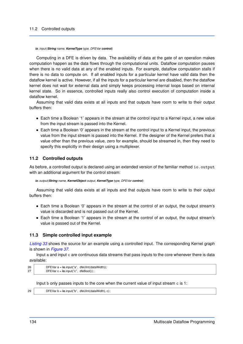
11.2 Controlled outputs
io . input(String name, KernelType type, DFEVar control)
Computing in a DFE is driven by data. The availability of data at the gate of an operation makescomputation happen as the data flows through the computational units. Dataflow computation pauseswhen there is no valid data at any of the enabled inputs. For example, dataflow computation stalls ifthere is no data to compute on. If all enabled inputs for a particular kernel have valid data then thedataflow kernel is active. However, if all the inputs for a particular kernel are disabled, then the dataflowkernel does not wait for external data and simply keeps processing internal loops based on internalkernel state. So in essence, controlled inputs really also control execution of computation inside adataflow kernel.
Assuming that valid data exists at all inputs and that outputs have room to write to their outputbuffers then:
• Each time a Boolean ‘1’ appears in the stream at the control input to a Kernel input, a new valuefrom the input stream is passed into the Kernel.• Each time a Boolean ‘0’ appears in the stream at the control input to a Kernel input, the previous
value from the input stream is passed into the Kernel. If the designer of the Kernel prefers that avalue other than the previous value, zero for example, should be streamed in, then they need tospecify this explicitly in their design using a multiplexer.
11.2 Controlled outputs
As before, a controlled output is declared using an extended version of the familiar method io.output
with an additional argument for the control stream:
io .output(String name, KernelObject output, KernelType type, DFEVar control)
Assuming that valid data exists at all inputs and that outputs have room to write to their outputbuffers then:
• Each time a Boolean ‘0’ appears in the stream at the control of an output, the output stream’svalue is discarded and is not passed out of the Kernel.• Each time a Boolean ‘1’ appears in the stream at the control of an output, the output stream’s
value is passed out of the Kernel.
11.3 Simple controlled input example
Listing 33 shows the source for an example using a controlled input. The corresponding Kernel graphis shown in Figure 37.
Input a and input c are continuous data streams that pass inputs to the core whenever there is dataavailable:
26 DFEVar a = io.input(”a”, dfeUInt(dataWidth));27 DFEVar c = io.input(”c” , dfeBool()) ;
Input b only passes inputs to the core when the current value of input stream c is 1:
29 DFEVar b = io.input(”b”, dfeUInt(dataWidth), c) ;
134 Multiscale Dataflow Programming

11. Controlled Inputs and Outputs
y
+
a
b
c
mux1 0
0
Figure 37: Kernel Graph featuring simple use of controlled input
When the Boolean value from input stream c is 0, the previous value of b passes into the core. Amultiplexer uses the control stream c to select between the current value of b or 0, and thus if c is 0then the output is a + 0 instead of a + b:
32 DFEVar result = a + (c ? b : 0);
11.4 Example for an input controlled by a counter
The control for an input or output does not have to derive from an input: input and output controls canalso be derived from internally generated streams such as counters. The output of a counter can bepassed to a comparator to generate the necessary Boolean stream.
Listing 34 shows an implementation of a Kernel that uses a counter to control one of its inputs.The first 10 values from the controlled input stream b are added to continuous stream a and output
in stream y. After the first 10 elements of a and b, the unmodified data from stream a is output in streamy.
We use a counter to output only the first 10 elements of stream b:
20 DFEVar readLimit = io.scalarInput(”readCount”, dfeUInt(32));21 DFEVar count = control.count.simpleCounter(32);22 DFEVar read = count < readLimit;2324 // Inputs25 DFEVar b = io.input(”b”, dfeUInt(32), read);
A multiplexer is used to select between adding either the first ten elements of b or zero (to give theunmodified value) to a:
29 DFEVar result = a + (read ? b : 0);
Multiscale Dataflow Programming 135

11.4 Example for an input controlled by a counter
Listing 33: Class with a simple controlled input (SimpleControlledInputKernel.maxj).1 /∗∗2 ∗ Document: MaxCompiler Tutorial (maxcompiler-tutorial.pdf)3 ∗ Chapter: 11 Example: 1 Name: Simple controlled Input4 ∗ MaxFile name: SimpleControlledInput5 ∗ Summary:6 ∗ Kernel design using a controlled input . Inputs a and c are continuous7 ∗ data streams that will pass inputs to the core whenever there is data8 ∗ available . Input b will only pass inputs to the core when the current9 ∗ value of input stream c is 1.
10 ∗/1112 package simplecontrolledinput;1314 import com.maxeler.maxcompiler.v2.kernelcompiler.Kernel;15 import com.maxeler.maxcompiler.v2.kernelcompiler.KernelParameters;16 import com.maxeler.maxcompiler.v2.kernelcompiler.types.base.DFEVar;1718 class SimpleControlledInputKernel extends Kernel {1920 private static final int dataWidth = 32;2122 SimpleControlledInputKernel(KernelParameters parameters) {23 super(parameters);2425 // Inputs26 DFEVar a = io.input(”a”, dfeUInt(dataWidth));27 DFEVar c = io.input(”c” , dfeBool()) ;2829 DFEVar b = io.input(”b”, dfeUInt(dataWidth), c) ;3031 // Logic32 DFEVar result = a + (c ? b : 0);3334 debug.simPrintf(”c: %d\n”, c);35 // Output36 io .output(”y” , result , dfeUInt(dataWidth));37 }38 }
The result is then written to y:
32 io .output(”y” , result , dfeUInt(32)) ;
WThe example uses a simple 32-bit counter for clarity, but this wraps when it reaches 232, sothe Kernel tries to read in another 10 elements from input stream b. A complex counter inSTOP AT MAX mode provides a more robust implementation that only ever reads in the first 10elements of b.
136 Multiscale Dataflow Programming

11. Controlled Inputs and Outputs
Listing 34: Class with a counter controlled input (CounterControlledInputKernel.maxj).1 /∗∗2 ∗ Document: MaxCompiler Tutorial (maxcompiler-tutorial.pdf)3 ∗ Chapter: 11 Example: 2 Name: Counter Controlled Input4 ∗ MaxFile name: CounterControlledInput5 ∗ Summary:6 ∗ Kernel design that uses a counter to control one of its inputs.7 ∗/89 package countercontrolledinput;
1011 import com.maxeler.maxcompiler.v2.kernelcompiler.Kernel;12 import com.maxeler.maxcompiler.v2.kernelcompiler.KernelParameters;13 import com.maxeler.maxcompiler.v2.kernelcompiler.types.base.DFEVar;1415 public class CounterControlledInputKernel extends Kernel {16 public CounterControlledInputKernel(KernelParameters parameters) {17 super(parameters);1819 // Control Counter20 DFEVar readLimit = io.scalarInput(”readCount”, dfeUInt(32));21 DFEVar count = control.count.simpleCounter(32);22 DFEVar read = count < readLimit;2324 // Inputs25 DFEVar b = io.input(”b”, dfeUInt(32), read);26 DFEVar a = io.input(”a”, dfeUInt(32)) ;2728 // Logic29 DFEVar result = a + (read ? b : 0);3031 // Outputs32 io .output(”y” , result , dfeUInt(32)) ;33 }34 }
ExercisesExercise 1: Counter-controlled input
Through the use of a counter-controlled input, create a Kernel design that merges two color images.The image blue.ppm is a 512x512 image that should serve as one input to the design. The other inputshould be the 256x256 image lena256.ppm. The output should be a 512 x 512 color image with the256x256 Lena image centered on the blue background. The output should look like Figure 38.
Note that the input image stream comes into the Kernel as a sequence of three color componentsper pixel, Red, Green and Blue, one component per Kernel tick.
A copy of the image shown in Figure 38 is provided in lena merged.ppm for comparison purposes.
Exercise 2: Controlled output
Take the image result file from Exercise 1. Through the use of a controlled output, discard 3 out of every4 pixels to produce an output that is the input image scaled to 256x256 size. For each group of fourpixels {(0,0), (1,0), (0,1), (1,1)}, only pixel (0,0) should be taken. The output should looklike Figure 39.
Multiscale Dataflow Programming 137

11.4 Example for an input controlled by a counter
Figure 38: Blue-Framed Lena Image
Figure 39: Scaled Lena Image
138 Multiscale Dataflow Programming

12On-chip FMem in Kernels
We are forced to recognize the possibility of constructing a hierarchy of memories, each ofwhich has greater capacity than the preceding, but which is less quickly accessible.
– John von Neuman
DFEs provide two basic kinds of memory: FMem and LMem. FMem (Fast Memory) is on-chip StaticRAM (SRAM) which can hold several MBs of data. Off-chip LMem (Large Memory) is implementedusing DRAM technology and can hold many GBs of data. The key to efficient dataflow implementationsis to choreograph the data movements to maximize the reuse of data while it is in the chip and minimizemovement of data in and out of the chip. In this section we address the use of FMem directly withinkernels.
All inputs and outputs to kernel memories are streams:
• Streams of addresses go in.
• Streams of data come out.
• Where data is being written, streams of data input go into the RAM.
Multiscale Dataflow Programming 139

12.1 Allocating, reading and writing FMem
Kernel memories have multiple streams in and out of the memory that can look at the same set ofdata in a single tick.
12.1 Allocating, reading and writing FMem
All kernel memory uses the same basic declaration, taking two arguments: the type of the data storedin the memory and the number of items to be stored. The method alloc returns a Memory object whichcan then be used to access the memory.
Memory<DFEVar> mem.alloc(DFEType type, int depth)
Memory is parameterized with a Java generic DFEVar indicating the type of stream that the memorywill retain. Memories can also contain composite kernel types in which case the appropriate alternativestring would be used (DFEVector, DFEComplex, etc).
Memory which is read and written is termed a RAM, while memory that is only read is termed aROM. Example uses for RAMs include storing a window into an input or output stream, state to bereused within a Kernel and reordering of data. Data can be written into a RAM via the call:
Memory.write(DFEVar address, DFEVar data, DFEVar enable)
The write method has three input streams: addresses to write to, the data to write to that addressand a 1-bit enable which indicates whether the write should be executed or not in that tick. The enableis vital to allow the programmer to selectively control what data is written into a RAM.
A second stream stream of outputs can be read from specified addresses in the RAM:
Memory.read(DFEVar address)
There are some restrictions on writing into memories. In particular:
• If you write to a memory address in a kernel tick you can not call read with the same address inthe same tick. Attempting to do so will return undefined data.
• You are limited to either a maximum of 2 calls to write and no calls to read on a memory, or 1call to write and any number of calls to read.
W The content of a memory is undefined when the dataflow engine is first loaded. Once thecontent is set by the user, the data in the memory persists when the Kernel is reset.
12.1.1 Memory example
Example 1 shows a memory used to reverse the order of data in an input stream. The Kernel source isshown in Listing 35.
The memory is declared to contain single-precision floating point numbers:
50 Memory<DFEVar> reverseRam = mem.alloc(dfeFloat(8,24), DATA SIZE);
Data is written into the memory using a call to write:
51 reverseRam.write(inputAddress, inputData, readingInput);
140 Multiscale Dataflow Programming

12. On-chip FMem in Kernels
The output is created with a read call:
52 DFEVar outputData = reverseRam.read(outputAddress);
The code in the example has two phases of operation:
Phase 1 : the input stream is written into the memory.
Phase 2 : the data is read out in reverse order from the memory.
A counter counts to twice the size of the data set stored in the memory. Dropping the most significantbit from the counter gives an incrementing address to each element in the memory to write the inputdata. Reversing this address gives a decrementing address to each element to read the data from thememory in reverse order. Data is written into the memory while the counter is less that the size of thememory. When the counter hits the size of the memory, the input stream is disabled and the contentsof the memory are written out to the output stream in reverse order.
W This example is not a general-purpose method for reversing an arbitrarily-sized input stream asit only reverses chunks of the stream that are the size of the memory.
W A useful function when working with memories is MathUtils.bitsToAddress(dataSize),which returns the number of bits required to address a memory of dataSize.
12.2 Using memories as read-only tables
One common use of kernel memories is to store tables of infrequently changing constants, for examplecoefficients, as Read-Only Memory (ROMs). This gives the equivalent behavior to using a large numberof constants and multiplexing between them, but is more space and performance efficient when thereare more than a few data items.
ROM tables can be initialized with contents specified either as an array of doubles or using Bits.
12.2.1 ROM example
Example 2 demonstrates the use of FMem as a ROM. The Kernel source for this example is shown inListing 36. This simple example takes an input stream of addresses and outputs the contents of theROM. The contents of the ROM are initialized with the first quarter of a sine curve using standard Javamath routines, by calling the setContents function.
A single read call generates an output from the memory. Multiple read calls with different addressinputs can return different values from the table in the same kernel tick.
12.2.2 Setting memory contents from the CPU
Memories can optionally be mapped, which allows them to be changed by the CPU at runtime, ideallywhen the kernel is inactive. Mapped memories are an alternative to setting memory contents at compile-time only, and are very useful for values that change slowly but sufficiently frequently that it would beundesirable to recompile the maxfile.
Multiscale Dataflow Programming 141

12.2 Using memories as read-only tables
Memories that are mapped to the CPU are declared with the same syntax as normal memories, butwith an additional call to declare a name which can be used by the CPU to set the memory contents.
Memory.mapToCPU(String name)
It is important to note that using a mapped memory is an alternative to setting the contents in thekernel, i.e. it is not valid to call both setContents and mapToCPU on the same memory. Mappedmemories should be initialized with contents from CPU code.
12.2.3 Mapped ROM example
Example 3 demonstrates the use of a mapped memory as a ROM with multiple reads. The Kernelsource for this example is shown in Listing 37. In this example, two input streams of addresses arepassed to read calls for the memory and the corresponding outputs are connected directly to thekernel’s output streams.
The following lines show the instantiation of the ROM and mapping it to the CPU with the name‘‘mappedRom’’:
27 Memory<DFEVar> mappedRom = mem.alloc(dfeFloat(8,24), dataSize);28 mappedRom.mapToCPU(”mappedRom”);
Once the memory is initialized, two calls to read are made and the results are connected to thekernel output streams:
31 DFEVar readA = mappedRom.read(addressA);32 DFEVar readB = mappedRom.read(addressB);3334 io .output(”outputA”, readA, dfeFloat(8,24)) ;35 io .output(”outputB”, readB, dfeFloat(8,24)) ;
The contents of the ROM are set in the CPU code by passing a pointer to the contents as anargument to the SLiC function for running the DFE.
The CPU code for this example is shown in Listing 38. A block of memory is allocated and then setup with the desired values; in this case our sine function:
69 double ∗romContents = malloc(sizeBytesDouble);
74 generateInputData(75 size,76 inAddressA, inAddressB,77 romContents, romContentsReversed);
The contents are then passed to the SLiC function:
80 DualPortMappedRom(81 size,82 inAddressA, inAddressB,83 outDataA, outDataB,84 romContents);
It is often useful to create custom SLiC engine interfaces to separate setting mapped memory valuesinto a specific initialization SLiC interface function and then not set them during the compute function(using the ignoreMem function on the engine interface object). This saves uploading identical valuesfor the mapped memory repeatedly every time the DFE runs a computation.
142 Multiscale Dataflow Programming

12. On-chip FMem in Kernels
12.3 Creating a memory port which both reads and writes
As an optimization, it is also possible to create a single memory port which both reads and writes in thesame tick using the same address:
DFEVar Memory.port(DFEVar address, DFEVar data in, DFEVar enable, RamWriteMode portMode)
A read-write port has input address, data and write-enable streams and an output data stream; theinput address stream is used for both the write and read locations. A read-write memory port alwaysoutputs data from the location specified in the input address stream, regardless of the status of thewrite-enable stream.
Read/write memory ports must be set with a RamWriteMode, which can either be READ FIRST orWRITE FIRST. This determines the behavior when data is read from and written in the same tick. InREAD FIRST mode, the existing contents of the memory location is read before being written over. InWRITE FIRST mode, the new value propagates directly to the output in the same tick as it is beingwritten. Not all DFE architectures support both modes.
WRamWriteMode applies only to determining whether the read or write should be performedfirst for this port, accessing the same address from another port will return undefined dataregardless of what mode is used.
12.4 Understanding memory resources
Kernel memories are implemented using a special on-chip memory resource. The amount of on-chipmemory used by an application can often be a determining factor in its performance, so it is worthunderstanding a little of how memories are built and what the costs of different operations are.
The number of on-chip BRAM resources required for a particular kernel memory depends on:
• The number of items in the memory (i.e. its depth).
• The type of the data held in the memory (i.e. its width).
• The number and type of ports.
In general, the larger the memory the more silicon area it will require. Memories with many portswill use also use more on-chip area because the basic storage element must be replicated to provideparallel access. A physical on-chip BRAM resource supports two ports, so if more ports are requested(e.g. many calls to the read function) then several instances of the resource will be automaticallyallocated to provide the correct level of access parallelism. The fact that BRAMs have 2 ports is alsothe source of the restriction that kernel memories with more than two ports must have at most one writeport, since the write data must be copied to all parallel memory instances.
In general, the amount of memory resource required in silicon for memories with only read portsscales with:
depth× width× (numreadports÷ 2)
For memories with 1 write port and many read ports, the silicon resource requirements are proportionalto:
depth× width× numreadports
Multiscale Dataflow Programming 143

12.4 Understanding memory resources
(a) Original image (b) Processed image
Figure 40: Original image and image after the coefficients have been applied.
ExercisesExercise 1: Simple ROM
In this exercise, a simple application is supplied that streams in a 256x256 pixel image in the sameformat as for the exercises in section 11: Controlled Inputs and Outputs. Modify this example to applya set of coefficients to each line of the image. There should be one coefficient for each pixel in a lineof the image. The coefficients should be floating-point numbers between 0.0 and 1.0. A suitable set ofcoefficients can be calculated using the equation:
ci =
{1.0− (1.0/(X/2))× ((X/2)− i) if i < X/21.0− (1.0/(X/2))× (i− (X/2)) if i ≥ X/2
Where ci is the coefficient for the ith pixel in a row and X is the width of a row in the image.Figure 40 shows the image before and after these coefficients have been applied.
W Remember that the input image stream comes into the Kernel as a sequence of three colorcomponents per pixel, Red, Green and Blue, one component per tick.
Exercise 2: Dual-port RAM
Modify the previous exercise to read in the coefficients from an input stream and store them in a RAM.Once the coefficients have been read into the RAM, start processing the input data stream using thesecoefficients as before. Use a separate input stream for the coefficients.
W It is important to control the input and output streams to ensure only correct data is read fromthe input streams and written to the output stream correctly.
144 Multiscale Dataflow Programming

12. On-chip FMem in Kernels
Listing 35: A memory used to reverse the data in an input stream (DualPortRamKernel.maxj).10 package dualportram;1112 import com.maxeler.maxcompiler.v2.kernelcompiler.Kernel;13 import com.maxeler.maxcompiler.v2.kernelcompiler.KernelParameters;14 import com.maxeler.maxcompiler.v2.kernelcompiler.stdlib.core.Count.Counter;15 import com.maxeler.maxcompiler.v2.kernelcompiler.stdlib.core.Count.Params;16 import com.maxeler.maxcompiler.v2.kernelcompiler.stdlib.memory.Memory;17 import com.maxeler.maxcompiler.v2.kernelcompiler.types.base.DFEVar;18 import com.maxeler.maxcompiler.v2.utils.MathUtils;1920 class DualPortRamKernel extends Kernel {21 DualPortRamKernel(KernelParameters parameters) {22 super(parameters);2324 int DATA SIZE = 16;2526 /∗Create a counter to generate the addresses to the RAM. This counts to twice the size of27 ∗ the data set stored in the RAM. ∗/28 int addrBits = MathUtils.bitsToAddress(DATA SIZE);29 Params addressCounterParams = control.count.makeParams(addrBits+1);30 Counter addressCounter = control.count.makeCounter(addressCounterParams);3132 /∗ Dropping the most significant bit from the counter gives us an incrementing address to33 ∗ each element in the RAM to write the input data. Reversing this address gives us a34 ∗ decrementing address to each element to read the data from the RAM in reverse order. ∗/35 DFEVar inputAddress = addressCounter.getCount();36 DFEVar outputAddress = DATA SIZE - 1 - addressCounter.getCount();3738 inputAddress = inputAddress.cast(dfeUInt(addrBits));39 outputAddress = outputAddress.cast(dfeUInt(addrBits));4041 // If the counter is less that the size of the RAM, then we are reading input data42 DFEVar readingInput = addressCounter.getCount() < DATA SIZE;4344 // Read input data during the first half of the counter45 DFEVar inputData = io.input(”inputData”, dfeFloat(8,24) , readingInput);4647 /∗ The input port takes the input address and data input stream. The write-enable is set48 ∗ to readingInput, which is true for the first half of the counter. ∗/49 // The output port takes the decrementing output address50 Memory<DFEVar> reverseRam = mem.alloc(dfeFloat(8,24), DATA SIZE);51 reverseRam.write(inputAddress, inputData, readingInput);52 DFEVar outputData = reverseRam.read(outputAddress);53 /∗ When the counter is in its second half, the contents of the RAM will be read out in54 ∗ reverse order. ∗/55 io .output(”outputData”, outputData, dfeFloat(8,24) , ˜readingInput);56 }57 }
Multiscale Dataflow Programming 145

12.4 Understanding memory resources
Listing 36: A memory used as a ROM, initialized with doubles (RomKernel.maxj).1 /∗∗2 ∗ Document: MaxCompiler Tutorial (maxcompiler-tutorial.pdf)3 ∗ Chapter: 12 Example: 2 Name: Rom Kernel4 ∗ MaxFile name: Rom5 ∗ Summary:6 ∗ Kernel design that demonstrates the use of a single port ROM.7 ∗/89 package rom;
1011 import com.maxeler.maxcompiler.v2.kernelcompiler.Kernel;12 import com.maxeler.maxcompiler.v2.kernelcompiler.KernelParameters;13 import com.maxeler.maxcompiler.v2.kernelcompiler.stdlib.memory.Memory;14 import com.maxeler.maxcompiler.v2.kernelcompiler.types.base.DFEVar;1516 class RomKernel extends Kernel {17 RomKernel(KernelParameters parameters) {18 super(parameters);1920 final int addrBits = 8;21 final int dataSize = ( int )Math.pow(2, addrBits);2223 // Input24 DFEVar address = io.input(”address”, dfeUInt(addrBits));2526 double contents[] = new double[dataSize];27 for ( int i = 0; i < dataSize; i++)28 contents[ i ] = Math.sin(((Math.PI/2.0)/dataSize)∗i) ;2930 Memory<DFEVar> table = mem.alloc(dfeFloat(8,24), dataSize);31 table .setContents(contents);3233 DFEVar result = table.read( address );3435 // Output36 io .output(”output” , result , dfeFloat(8, 24));37 }38 }
146 Multiscale Dataflow Programming

12. On-chip FMem in Kernels
Listing 37: A mapped memory used as ROM, with two simultaneous reads (DualPortMappedRomKer-nel.maxj).1 /∗∗2 ∗ Document: MaxCompiler Tutorial (maxcompiler-tutorial.pdf)3 ∗ Chapter: 12 Example: 3 Name: Dualport mapped ROM4 ∗ MaxFile name: DualPortMappedRom5 ∗ Summary:6 ∗ Kernel design that demonstrates the use of a dual port mapped ROM.7 ∗/89 package dualportmappedrom;
1011 import com.maxeler.maxcompiler.v2.kernelcompiler.Kernel;12 import com.maxeler.maxcompiler.v2.kernelcompiler.KernelParameters;13 import com.maxeler.maxcompiler.v2.kernelcompiler.stdlib.memory.Memory;14 import com.maxeler.maxcompiler.v2.kernelcompiler.types.base.DFEVar;15 import com.maxeler.maxcompiler.v2.utils.MathUtils;1617 class DualPortMappedRomKernel extends Kernel {18 DualPortMappedRomKernel(KernelParameters parameters, int dataSize) {19 super(parameters);2021 int addrBits = MathUtils.bitsToAddress(dataSize);2223 // Input24 DFEVar addressA = io.input(”addressA”, dfeUInt(addrBits));25 DFEVar addressB = io.input(”addressB”, dfeUInt(addrBits));2627 Memory<DFEVar> mappedRom = mem.alloc(dfeFloat(8,24), dataSize);28 mappedRom.mapToCPU(”mappedRom”);2930 // Output31 DFEVar readA = mappedRom.read(addressA);32 DFEVar readB = mappedRom.read(addressB);3334 io .output(”outputA”, readA, dfeFloat(8,24)) ;35 io .output(”outputB”, readB, dfeFloat(8,24)) ;36 }37 }
Multiscale Dataflow Programming 147

12.4 Understanding memory resources
Listing 38: Main function for CPU code demonstrating setting of a mapped ROM (DualPortMappe-dRomCpuCode.c).
61 int main()62 {63 const int size = 256;64 int sizeBytesFloat = size ∗ sizeof(float ) ;65 int sizeBytesDouble = size ∗ sizeof(double);66 int sizeBytesInt = size ∗ sizeof( uint8 t ) ;67 uint8 t ∗inAddressA = malloc(sizeBytesInt);68 uint8 t ∗inAddressB = malloc(sizeBytesInt);69 double ∗romContents = malloc(sizeBytesDouble);70 double ∗romContentsReversed = malloc(sizeBytesDouble);71 float ∗outDataA = malloc(sizeBytesFloat);72 float ∗outDataB = malloc(sizeBytesFloat);7374 generateInputData(75 size,76 inAddressA, inAddressB,77 romContents, romContentsReversed);7879 printf ( ”Running DFE.\n”);80 DualPortMappedRom(81 size,82 inAddressA, inAddressB,83 outDataA, outDataB,84 romContents);8586 int status = check(87 size,88 outDataA, outDataB,89 romContents, romContentsReversed);9091 if (status)92 printf ( ”Test failed .\n”) ;93 else94 printf ( ”Test passed OK!\n”);9596 return status;97 }
148 Multiscale Dataflow Programming

13Talking to CPUs, Large Memory (LMem),and other DFEs
A Dataflow Engine needs to communicate with its LMem (Large Memory, GBs of off-chip memory),CPUs and other DFEs. The Manager in a dataflow program describes the choreography of data move-ment between DFEs, connecting CPUs, and also the GBs of data in LMem.
Figure 41 illustrates the architecture of a Maxeler acceleration system which comprises dataflowengines (DFEs) attached directly to local memories and to a CPU. In a Maxeler solution, there may bemultiple dataflow engines connected together via high-bandwidth MaxRing interconnect. A dataflowengine is made up of one or more Kernels and a Manager. Within a Kernel, streams provide a pre-dictable environment for the designer to concentrate on data flow and arithmetic. Managers provide apredictable input and output streams interface to the Kernel.
MaxCompiler provides pre-configured Managers, including the Standard Manager, and the Man-ager Compiler for creating complex Managers of your own.
The Manager Compiler allows you to create complex Manager designs, with multiple Kernels andcomplex interaction between Kernels and with IO resources. The Manager Compiler Tutorial docu-ment, also provided with MaxCompiler, covers the Manager Compiler in detail.
Multiscale Dataflow Programming 149
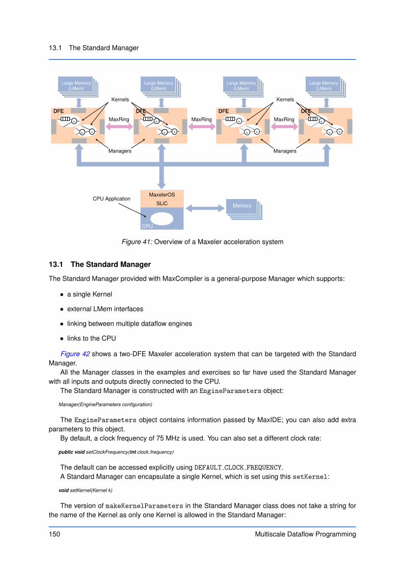
13.1 The Standard Manager
MaxelerOSSLiC Memory
CPU
DFE
*+
+
CPU Application
MaxRingDFE
*+
+
DFE
*+
+
DFE
*+
+
*+
+
*+
+ MaxRing MaxRing
Kernels
Managers
Kernels
Managers
DFE DFE DFE DFE
Large Memory(LMem)
Large Memory(LMem)
Large Memory(LMem)
Large Memory(LMem)
Figure 41: Overview of a Maxeler acceleration system
13.1 The Standard Manager
The Standard Manager provided with MaxCompiler is a general-purpose Manager which supports:
• a single Kernel
• external LMem interfaces
• linking between multiple dataflow engines
• links to the CPU
Figure 42 shows a two-DFE Maxeler acceleration system that can be targeted with the StandardManager.
All the Manager classes in the examples and exercises so far have used the Standard Managerwith all inputs and outputs directly connected to the CPU.
The Standard Manager is constructed with an EngineParameters object:
Manager(EngineParameters configuration)
The EngineParameters object contains information passed by MaxIDE; you can also add extraparameters to this object.
By default, a clock frequency of 75 MHz is used. You can also set a different clock rate:
public void setClockFrequency(int clock frequency)
The default can be accessed explicitly using DEFAULT CLOCK FREQUENCY.A Standard Manager can encapsulate a single Kernel, which is set using this setKernel:
void setKernel(Kernel k)
The version of makeKernelParameters in the Standard Manager class does not take a string forthe name of the Kernel as only one Kernel is allowed in the Standard Manager:
150 Multiscale Dataflow Programming

13. Talking to CPUs, Large Memory (LMem), and other DFEs
Kernel
Manager
DFE
LMem
*+
DFE
*+
MaxRing
LMem
*+ *+ *+ *+
MaxelerOSSLiC Memory
CPU
CPU Application
MAXRING M
AXRING
LMEM
CPUCPU
LMEM
Figure 42: Two-chip acceleration system using the Standard Manager
public KernelParameters makeKernelParameters()
setIO allows you to link the input and output streams in the Kernel to I/O resources enabled by theManager:
void setIO(Manager.IOType io type)void setIO(IOLink ... links )
The first version of the function allows all inputs and outputs to be set together. All the links havebeen to the CPU in the examples so far, for example:
Manager m = new Manager(new EngineParameters(args));m.setIO(IOType.ALL CPU);
Figure 43 illustrates how a Manager, Kernel and CPU interact with one input and one output bothset to CPU.
Another option for setting all of the I/Os together is NOIO:
Manager m = new Manager(new EngineParameters(args));m.setIO(IOType.NOIO);
This builds the Kernel as a block of logic with no connections to the outside world. This is usefulfor determining the performance of a Kernel in isolation from the rest of the logic and optimization. ABuildConfig object (see subsubsection 13.4.1) with the build level set to FULL BUILD cannot be usedin this mode.
The link for each input and output stream in the Kernel can be specified individually using a list ofIOLinks. An IOLink is declared using a stream name and the corresponding link type:
IOLink link (String io name, IOLink.IODestination iotype)
Multiscale Dataflow Programming 151

13.2 MaxRing communication
MaxelerOSSLiC
CPUdataOutdataIn
CPUapplication
DFE
Kernel
Manager
in out
CPU
Figure 43: All CPU links on a Standard Manager
iotype can be one of:
• CPU connects the stream to the CPU
• MAXRING A or MAXRING B connects the stream to one of two, bi-directional MaxRing links on aMAX3
• LMEM LINEAR 1D connects the stream to LMem with a linear address generator
• LMEM BLOCKED 3D connects the stream to LMem with a 3D address generator
13.2 MaxRing communication
The MaxRing interconnect allows data to be transferred at high speed directly between dataflow en-gines. Each dataflow engine in the system has a direct bidirectional connection to up to two otherDFEs, as shown in Figure 41.
There are two MaxRing connections on a MAX3: MAXRING A and MAXRING B.
152 Multiscale Dataflow Programming

13. Talking to CPUs, Large Memory (LMem), and other DFEs
Listing 39: Inter-chip loopback Kernel (MaxringKernel.maxj).1 /∗∗2 ∗ Document: MaxCompiler Tutorial (maxcompiler-tutorial.pdf)3 ∗ Chapter: 13 Example: 1 Name: Maxring4 ∗ MaxFile name: Maxring5 ∗ Summary:6 ∗ Kernel design that takes a scalar input to select whether7 ∗ it should behave as the left or right DFE.8 ∗/9
10 package maxring;1112 import com.maxeler.maxcompiler.v2.kernelcompiler.Kernel;13 import com.maxeler.maxcompiler.v2.kernelcompiler.KernelParameters;14 import com.maxeler.maxcompiler.v2.kernelcompiler.types.base.DFEVar;1516 class MaxringKernel extends Kernel {1718 MaxringKernel(KernelParameters parameters) {19 super(parameters);2021 DFEVar isLeft = io.scalarInput( ” isLeft ” , dfeBool()) ;2223 DFEVar inA = io.input(”inA”, dfeUInt(32), isLeft ) ;24 DFEVar inB = io.input(”inB”, dfeUInt(32), ˜ isLeft ) ;2526 io .output(”outA”, inA, dfeUInt(32), isLeft ) ;27 io .output(”outB”, inB, dfeUInt(32), ˜ isLeft ) ;28 }29 }
13.2.1 Example with loop-back across two chips
Example 1 shows a simple application that reads a stream of data from the CPU into one dataflowengine, passes the data over a MaxRing link to the second DFE and then writes the data back from thesecond DFE to the CPU. Listing 39 shows the source code for the Kernel.
As both dataflow engines are identically configured, the Kernel takes a scalar input to select whetherit should behave as the left or right DFE in Figure 44:
21 DFEVar isLeft = io.scalarInput( ” isLeft ” , dfeBool()) ;
The inputs and outputs are controlled by isLeft to either read from inA and write to outA, or readfrom inB and write to outB:
23 DFEVar inA = io.input(”inA”, dfeUInt(32), isLeft ) ;24 DFEVar inB = io.input(”inB”, dfeUInt(32), ˜ isLeft ) ;2526 io .output(”outA”, inA, dfeUInt(32), isLeft ) ;27 io .output(”outB”, inB, dfeUInt(32), ˜ isLeft ) ;
Figure 45 shows the resultant Kernel graph for the example.The Manager connects the inputs and outputs to the CPU and MaxRing links:
30 m.setIO(link( ”inA”, CPU), link( ”inB”, MAXRING A),31 link ( ”outA”, MAXRING A), link(”outB”, CPU));
Multiscale Dataflow Programming 153

13.3 Large Memory (LMem)
MaxelerOSSLiC
CPU
Kernel
Host application
DFEMaxRing
DFE MAXRING_A M
AXRING_A
CPUCPU
inA outA
i_data o_data
inB outB
Left Right
Manager
Figure 44: MaxRing links on a Standard Manager
13.3 Large Memory (LMem)
The Standard Manager allows you to connect any number of streams to the LMem on the dataflowengine. This allows large amounts of data to be kept local to the dataflow engine and iterated over. TheLMem appears as one contiguous piece of memory. There are different access patterns available forthe memory:
• LMEM LINEAR 1D connects the stream to LMem with a simple linear address generator.
• LMEM BLOCKED 3D connects the stream to LMem with a 3D address generator.
The Manager Tutorial covers more advanced LMEM LINEAR 1D and LMEM BLOCKED 3D usage, aswell as other memory access patterns such as LMEM STRIDED 2D.
In the Standard Manager, each stream has its own address generator. The parameters for thebehavior of the memory address generators for each stream can be set up either in the CPU code or ina SLiC engine interface to simplify the CPU interface to the DFE.
The Standard Manager provides a CPU input stream called "write lmem" and an output streamto the CPU called "read lmem" for accessing the LMem linearly in the CPU software. MaxCompilerautomatically creates two SLiC engine interfaces, <.max file name> writeLMem and <.max file
name> readLMem, to write to and read from the LMem from the CPU using these streams.The memory controller and its address generators work in bursts. The burst length can be retrieved
in CPU code through SLiC:
int max get burst size(max file t ∗ const maxfile,const char ∗ const name);
154 Multiscale Dataflow Programming

13. Talking to CPUs, Large Memory (LMem), and other DFEs
inA
outBcontrol data
isLeft
not
inB
outA
Figure 45: Kernel for the simple MaxRing loopback
The burst length is also available in the Manager through the getBurstLength method.
W All dimensions provided as arguments to address generator functions are in bytes and must bea multiple of the burst length.
13.3.1 Linear address generators
A linear address generator is set up using two arguments address and size to address a block ofLMem, for example in a SLiC engine interface:
public void setLMemLinear(String streamName,InterfaceParam address,InterfaceParam size)
setLMemLinear reads size bytes from address, then returns to address to start reading again.
13.3.2 3D blocking address generators
A 3D Blocking address generator operates in a coordinate system where the unit of size in each di-mension is in bytes. A block of size (rwSizeFast, rwSizeMed, rwSizeSlow), with its origin at (offset-Fast,offsetMed,offsetSlow) is read from a larger block of size (arraySizeFast, arraySizeMed, arraySizeS-low):
public void setLMemBlocked(String streamName,long address,long arraySizeFast,long arraySizeMed,long arraySizeSlow,long rwSizeFast,long rwSizeMed,long rwSizeSlow,
Multiscale Dataflow Programming 155

13.3 Large Memory (LMem)
offset(f,m,s)
rwSizeFast
rw(m)
rw(s)
arraySizeFast arrayS
izeSlow
arra
ySizeM
ediu
m
Figure 46: 3D Blocking Address Generator, where offset(f,m,s) is the point (offsetFast, offsetMed, off-setSlow), rw(m) is rwSizeMed and rw(s) is rwSizeSlow
long offsetFast,long offsetMed,long offsetSlow)
The terms fast, medium and slow refer to the speed of indexing the LMem in that dimension: themost efficient access to the LMem indexes in the fast dimension first, then the medium, then the slow.
Figure 46 shows the meaning of the arguments in 3D space.
13.3.3 Large Memory (LMem) example
This example shows a Kernel with two inputs connected to LMem and an output to LMem. There areno inputs or outputs to the CPU from the Kernel.
In this example, the two input streams are read from different locations in memory, added togetherand written back to a third location. The input data is written directly from the CPU code via the"write lmem"stream before the Kernel runs and the output data is read back via the "read lmem"
stream once the Kernel has completed. Figure 47 shows the interaction of the Kernel, Manager andCPU code.
The body of the Kernel simply connects the output stream to the sum of the two input streams:
20 DFEVar inA = io.input(”inA”, dfeUInt(32)) ;21 DFEVar inB = io.input(”inB”, dfeUInt(32)) ;2223 io .output(”oData”, inA+inB, dfeUInt(32)) ;
156 Multiscale Dataflow Programming

13. Talking to CPUs, Large Memory (LMem), and other DFEs
DFE LMEM
CPU
CPUApplication
Kernel
Manager
inA inB
LMem
oData
MaxelerOSSLiC
CPU
Figure 47: LMem links on a Standard Manager
The Manager attaches the three streams to linear memory address generators:
32 m.setIO(link( ”inA”, IODestination.LMEM LINEAR 1D),33 link ( ”inB”, IODestination.LMEM LINEAR 1D),34 link ( ”oData”, IODestination.LMEM LINEAR 1D));
The CPU code first creates two buffers of data:
33 int32 t ∗inA = malloc(sizeBytes);34 int32 t ∗inB = malloc(sizeBytes);3536 for ( int i = 0; i < size; i++) {37 inA[ i ] = i ;38 inB[ i ] = size − i ;39 }
The two buffers are written to two separate locations in the LMem:
42 LMemLoopback writeLMem(0, sizeBytes, inA);43 LMemLoopback writeLMem(sizeBytes, sizeBytes, inB);
To run the Kernel, the default SLiC engine interface can be run:
45 printf ( ”Running DFE.\n”);46 LMemLoopback(size);
The SLiC function returns once the Kernel has completed writing its output to the LMem. Now the
Multiscale Dataflow Programming 157

13.4 Building DFE configurations
contents of the LMem at the output stream location can be read back to the CPU:
49 int32 t ∗outData = malloc(sizeBytes);50 LMemLoopback readLMem(2 ∗ sizeBytes, sizeBytes, outData);
13.4 Building DFE configurations
All Managers extend the maxcompiler.v1.managers.DFEManager class which provides several meth-ods. Specific Managers have additional methods.
abstract void build()
build launches the build process. It can be called only once.
void logMsg(String msg, Object... args)void logWarning(String msg, Object... args)
logMsg and logWarning allow you to log messages that are output in the build.log file in thebuild directory. This is preferable to printing directly to the console as these messages are saved forreference. Messages are formatted using a printf-like format.
makeKernelParameters is required for constructing a Kernel and supplies the name:
KernelParameters makeKernelParameters(String kernel name)
BuildConfig objects are useful for controlling the configuration of the build process:
BuildConfig getBuildConfig()void setBuildConfig(BuildConfig build config )
13.4.1 BuildConfig objects
A BuildConfig object can be used to set and retrieve build settings. Methods available includesetBuildEffort:
void setBuildEffort (BuildConfig. Effort effort )
Build effort tells the third party tools how much effort to put into trying to find an implementation of thecircuit to meet the design requirements (clock speed and area). The options available are HIGH, LOW,MEDIUM, VERY HIGH. Though it may be tempting to always run with high effort levels, builds can take along time when constraints are tight, so lower effort levels are useful for iterative test and optimization.
void setBuildLevel(BuildConfig.Level level )
Build level tells MaxCompiler up to which stage to run the build process. By default, MaxCompilerruns the complete build process and produces a .max file. Options available are:
• FULL BUILD (default) runs the complete process
• COMPILE ONLY stops after producing the VHDL output from MaxCompiler
• SYNTHESIS compiles the VHDL output
• MAP maps the synthesized design to components in the silicon device
• PAR places and routes the design for the chip, producing a DFE configuration
158 Multiscale Dataflow Programming

13. Talking to CPUs, Large Memory (LMem), and other DFEs
Levels other than FULL BUILD are typically only useful when debugging a build-related problem.Multi-pass Place and Route (MPPR) is the term used for automatically running the place and route
process on the same input design multiple times with different starting conditions in order to see whichrun gives the best results. setMPPRCostTableSearchRange instructs the silicon vendor’s map andplace and route tools to use a range of “cost tables” to initialize a multi-pass run:
void setMPPRCostTableSearchRange(int min, int max)
MaxCompiler can produce a timing report based on the output of the place and route tools. Thiscan be used to identify timing issues which may help when optimizing the design. Timing reports areenabled by default but can be enabled and disabled explicitly:
void setEnableTimingAnalysis(boolean v)
ExercisesExercise 1: LMem and MaxRing loop-back
Using the two examples in this section for help, write an application using two devices where:
1. The first device reads data from CPU and passes it to the other via an inter-chip link.
2. The second device reads data from the MaxRing link and writes it to LMem.
3. The CPU code reads the data from LMem and checks it against the input.
Figure 48 shows the required flow of data through the system.
Multiscale Dataflow Programming 159

13.4 Building DFE configurations
inAoutA
MaxelerOSSLiC
CPU
Kernel
CPU Application
i_data
Left
Manager
Memory
Right
inBoutB
LMem
DFE DFEMaxRing
MAXRING_A M
AXRING_A
LMEM
CPUCPU
LMEM
Figure 48: Exercise required data flow from CPU, via MaxRing links, to LMem
160 Multiscale Dataflow Programming

AJava References
For further information on the Java language we recommend the following resources:
• http://docs.oracle.com/javase/tutorial/java/index.html
An overview of Java and an introduction to its major syntactical features.
• http://docs.oracle.com/javase/tutorial/collections/index.html
An overview of the Java “Collections” API which is used often in MaxCompiler interfaces.
• http://docs.oracle.com/javase/6/docs/api/
API documentation for the standard Java libraries.
• http://www.java-tips.org/java-se-tips/java.lang/using-the-varargs-language-
feature.html
Introduction to using variable-argument methods in Java which are also common in MaxCompilerinterfaces.
Multiscale Dataflow Programming 161

162 Multiscale Dataflow Programming

BOn Multiscale Dataflow Research
– Oskar Mencer and Maxeler Advisors, December 2012
Once upon a time: http://www.cs.berkeley.edu/~kubitron/asplos98/abstracts/oscar_mencer.ps
Today, Multiscale Dataflow combines static dataflow computing on Dataflow Engines (DFEs) withoptimization on multiple levels of abstraction and scale: from mathematics and algorithms all the way toarithmetic and logic gates. Such vertical optimization is needed for mission-critical computations whereevery second counts. Being part of MAX-UP opens up a wide range of opportunities to investigate the-ory and practice of computing at the physical limits of a given generation of technology. This documentis intended for the seasoned MAX-UP researcher, writing papers based on MPC systems and lookingfor interdisciplinary research and new funding opportunities to advance multiscale dataflow computing.For Maxeler publications see: http://www.maxeler.com/publications/
Multiscale Dataflow Programming 163

1 Multiscale Dataflow Computing
1 Multiscale Dataflow Computing
Multiscale Dataflow Computing addresses the requirements of very large datasets and computationallyintensive problems on these datasets. We get a lot of requests to clarify which applications dataflowcomputing is most suitable for and how an FPGA chip compares to some multi-core chip running asmall loop-nest with a small dataset. However, instead of comparing chips, or suitability of algorithms,the key to meaningful investigation is to ask which problem sizes best balance the dataflow computationgiven a full system configuration, including multiple nodes with storage, networking and compute units.The hard part for researchers is to get a meaningfully large dataset. In the example referenced below,we show 3D finite difference running on a Maxeler 1U compute node with 4-8 dataflow engines (DFEs),and find that speedup with MPC systems grows with problem size, especially for large problems beyonda mesh with 10003 points.
[FD modeling beyond 70Hz with FPGA acceleration. D. Oriato, O. Pell (Maxeler), C. Andreolettiand N. Bienati (ENI). Society of Exploration Geophysicists 2010, Denver, USA, Oct. 2010]
2 Algorithm Transformation
So what else could one do to publish (not perish)? There are many opportunities to explore algorithmtransformations. A question rich in research potential is: How could this algorithm be transformed torun optimally on the particular system configuration. In essence, a multiscale dataflow machine bringswith it a vast space for developing novel versions of many existing algorithms. Even algorithms thatso far have not been popular are getting a new chance to shine. Following common folklore, one canalways trade off FFTs with convolutions in the time domain. And dataflow machines really excel at theconvolution, but there are a few notable exceptions depending on the size of the FFT and the amountof computation involved. Back to our example with 3D finite difference, there is flexibility in designingstencils of different shapes (locations of coefficients for the convolution). A significant project at Stanfordshowed how a cube stencil brings a 5x advantage over the star stencil, even though the star stencil isoptimal on a CPU.
[Accelerating 3D Convolution using Streaming Architectures on FPGAs. H. Fu, R. G. Clapp,O. Mencer and O. Pell. (Stanford University, Imperial College London, Maxeler Technologies), 79thSociety of Exploration Geophysicists (SEG), Houston, October 2009.]
3 From Bits to Numbers
Of course all this is only the tip of the iceberg. Considering the representation of data (how do youuse zeros and ones to describe all the other numbers), it may well be possible to invent new waysto design the data structures and arrange the layout and access of numbers in memory. By findinginnovative ways to streamline dataflow memory accesses, DFE technology can really flex its muscle.And data layout is just the beginning. The encoding of arrays of numbers can be investigated byencoding each array differently: Are there ways to compress the data or expand the data in order toachieve further acceleration? The famous examples here are gigantic sparse matrix computations inthe Finite Elements (FE) method, where the same shaped sparse matrix has to be read and writtenover and over and over again. Imagine if one had a memory controller that specializes in reading andwriting this particular sparse matrix in compressed form.
[Surviving the End of Scaling of Traditional Microprocessors in HPC. O. Lindtjrn, R. G. Clapp,O. Pell, O. Mencer and M. J. Flynn. (Schlumberger,Stanford University,Maxeler Technologies) IEEEHOT CHIPS 22, Stanford, USA, August 2010.]
164 Multiscale Dataflow Programming

B. On Multiscale Dataflow Research
4 Memory o’Memory
Making computation happen quicker is all about joint layout of data and compute modules. The researchchallenge starts when the data structures do not support controlling memory accesses, making memoryaccess “random”. But memory controllers cannot help with random memory access, or can they? Forirregular memory access issues such as applications with graph data structures, a top research ques-tion is: How can we expand the data by, for example, looking at the adjacency matrix representationor a sorted array representation of nodes and put all that together with metadata about location in thegraph. We could do all that without pointer-based linked-nodes which create all the “random” memoryaccesses. Since a dataflow machine is all about data and memory, using more memory (redundancy)to regularize (or regularise) memory access is a counter intuitive transformation with significant poten-tial. All such new memory layouts offer wide design spaces with wide opportunities for advancing ourunderstanding of algorithms and computation in general.
[Accelerating Unstructured Mesh Computations using Custom Streaming Architectures. KyryloTkachov, Supervisor: Prof. Paul H J Kelly (Imperial College London)]
5 Adapting Models to Dataflow
Let us also consider the reason to compute in the first place. Looking at the objective of the computationrather than a particular implementation, how can we attack a much more ambitious objective given thecapabilities of the dataflow systems? Is it possible to add more “Physics”, a more compute-intensiveapproximation method, or try to achieve a leap in capability? Just assuming that our 3D finite differenceis solving an acoustic wave equation clearly limits the potential research of solving the underlying partialdifferential equation. Looking at the overarching objective of creating 3D images of the earth, scientistscontemplate the use of the elastic wave equation which models the world a lot more accurately, oreven add viscosity to arrive at the visco-acoustic/elastic equations. It turns out that dataflow machinesbecome more and more attractive the more complexity becomes available, offering the possibility toaccelerate the development of next generation models and science in general. Writing a paper aboutPhysics models requires collaboration between scientists developing models and computer engineeringresearchers. Such collaboration offers substantial gain but it is no small political challenge in any(academic) environment. One of the goals of MAX-UP is to support and facilitate such interdisciplinarycollaboration.
[Beyond Traditional Microprocessors for Geoscience High-Performance Computing Applica-tions. O. Lindtjrn, R. G. Clapp, O. Pell, O. Mencer, M. J. Flynn and H. Fu. (Schlumberger, Stan-ford,Maxeler,Tsinghua University), IEEE Micro, vol. 31, no. 2, March/April 2011.]
6 Numerics
The most discrete field in computational research lies in numerics. Contributing to the understandingof interaction between number representation and convergence of algorithms, number of iterationsneeded, and accuracy of inputs and final results, may not be an entirely un-useful endeavor, helpingscientists to better understand their problems but also making a statement about the appropriatenessand stability of their results. What does this really mean? On the simple end, it is possible to explorevarious number representations such as variable bitwidths for floating point or fixed point (challengingmany proponents of the rigid IEEE floating point standards by using sub-single precision and super-quad precision). To further shrink the representation, we have block floating point with one exponent fora block of mantissa values, logarithmic numbers, all the way to mixed approaches minimizing bitwidthcombined with statistical methods, such as in for example:
Multiscale Dataflow Programming 165

7 Arithmetic
[A Mixed Precision Monte Carlo Methodology for Reconfigurable Accelerator Systems. Chow,Tse, Jin, Luk, Thomas, Leong, (Imperial, Sydney), FPGA 2012]
7 Arithmetic
Tightly coupled with representation we have arithmetic, and in that case, the space for research ex-ploration contains yet many more alternatives and options. If we add elementary function evaluations,we can ask the question which precision and range is needed for input and output respectively, andgiven a function, there is some optimal architecture that provides the desired result while minimizinglatency, area or arithmetic units. Of course, the same brute force design space exploration also appliesto higher-level functions and whole implementations of algorithms.
[Optimizing Hardware Function Evaluation Dong-U Lee, Altaf Abdul Gaffar, Oskar Mencer, WayneLuk (Imperial College) IEEE Transactions on Computers. vol. 54, no. 12, pp. 1520-1531. Dec, 2005.]
8 Precision and convergence
For some datasets there are issues of convergence of results when iterating millions of times in anumerical solver, which occasionally arise in some number representations and certain meshing strate-gies and not in others. On the other hand, some convergence issues might only arise after thousands ofiterations, which may take too long on conventional computers but can be reached on an MPC system.Investigating convergence goes hand-in-hand with minimizing precision and optimizing rounding. Thethird dimension is discretization in time and space: length of time-steps of simulations and the shape ofthe grid that we are computing the simulation on. The opportunity here is to study the interaction andcorrelations between precision, discretization in time and space, and convergence of the algorithm. Inparticular, there is scope to study application specific precision and rounding methods (in space, timeand value) based on domain specific criteria for the quality of results, to maximize dataflow computa-tion and provide further levers to better understand the implications of computing digitally in an analogworld.
[Stanford Seminar EE380: Flexible Number Representations for Computing with FPGAshttp://www.stanford.edu/class/ee380/ay0304.html, April 2004.]
9 Domain Specific Languages
Programming DFEs is intellectually stimulating. But how about making it even more exciting by addingDomain Specific Languages (in the spirit of our Finite Difference Compiler)? Or investigating directdataflow compilation from MATLAB or OpenCL or even Excel? Or translating and mapping establishedopen source software to a hyperfast platform? Of course, the ultimate challenge is to devise an au-tomatic or semi-automatic translation of sequential programs to dataflow, or even translation dynamicobject files of applications as they are running.
[Building Deep, Hazard-free Hardware Pipelines from OpenCL Programs Stanislaw Czerni-awski, MEng Thesis, Department of Computing Imperial College London (Supervised by Paul H J Kellyand Wayne Luk).]
10 Comparisons
Finally, if there is no way to avoid comparing technologies, we believe that the fair approach is to fixthe size of the machine (lets say to 1U), for example a 1U MPC-X dataflow appliance, and compareperformance and power consumption to a 1U machine from other vendors. Of course, the problem sizeneeds to be significant enough to justify dataflow computing. Alternatively, one can look at larger scale
166 Multiscale Dataflow Programming
B. On Multiscale Dataflow Research
systems with multiple nodes and normalize to the 1U space unit. Furthermore, one can normalize topower consumption, and compare large problem performance per Watt, as long as the power mea-surement is done at the power socket and not based on some artificial measure of power consumptioninside the chip. Finally, another perspective can be obtained by looking at what performance $1M canbuy, and then compare the performance and electricity and real-estate costs of the resulting machinesover a typical 3 year lifetime. Buying multi-core processors for $1M could bring another $1M in electric-ity costs, while buying a dataflow machine for $1M reduces electricity costs to under $100K AND thedataflow machine is faster. How can that be?
Multiscale Dataflow Programming 167

SLiC API Index
max actions free, 118max actions init, 117max actions t, 117, 118
max disable validation, 120
max errors check, 130max errors mode, 130max errors t, 129max errors trace, 130
max get mem double, 119max get mem uint64t, 119max get offset auto loop size, 119max get stream distance, 119
max ignore block, 120max ignore kernel, 120max ignore mem, 120max ignore mem input, 120max ignore mem output, 120max ignore offset, 120max ignore route, 120
max load, 112, 113max load array, 114max load group, 115
max lock any, 116
max get burst size, 154max watch range, 55MAXOS EXCLUSIVE, 115–117MAXOS SHARED, 115–117MAXOS SHARED DYNAMIC, 115–117
max nowait, 128, 129
max ok, 130
max queue input, 118max queue output, 118
max run array, 120max run array nonblock, 128max run group, 120max run group nonblock, 128max run nonblock, 128max run t, 128
max set mem double, 119max set mem uint64t, 119max set offset, 119max set param array double, 118max set param array uint64t, 118
168 Multiscale Dataflow Programming

SLIC API INDEX
max set param double, 117max set param uint64t, 117max set ticks, 119
max unload array, 114max unload group, 116max unlock, 116
max wait, 128
Multiscale Dataflow Programming 169
MaxJ API Index
!, 81!=, 80!==, 80*, 80*=, 80+, 80++, 81+=, 80-, 80--, 81/, 80<, 29, 80<<, 80<=, 80<==, 80=, 80==, 80===, 80>, 29, 80>=, 80>>, 80>>=, 80>>>, 80?:, 28, 80, 81, 93[], 80, 127
%, 81&, 29, 80, 81&&, 81*=, 80+=, 80>>=, 80^, 80~, 80|, 80, 81||, 81
addConstant, 126addMaxFileConstant, 127addMaxFileDoubleConstant, 127addMaxFileStringConstant, 127addParam, 124addParamArray, 127alloc, 140
Bits, 141build, 158build(), 42BuildConfig, 151, 158BuildConfig.Effort, 158BuildConfig.Level, 158
cast, 74
170 Multiscale Dataflow Programming
MAXJ API INDEX
COMPILE ONLY, 158control.count, 101control.count.makeCounterChain, 103control.count.simpleCounter, 29, 84control.mux, 28, 93count.makeCounter, 106count.makeParams, 105Count.Params, 105, 106COUNT LT MAX THEN WRAP, 105Counter, 106CounterChain, 103, 104CPU, 152CPUTypes, 124createSLiCinterface, 121
DEFAULT CLOCK FREQUENCY, 150dfeBool, 73, 80DFEComplex, 75, 78DFEComplexType, 72, 75, 78, 80DFEFix, 74, 75, 80dfeFixOffset, 72DFEFloat, 71, 72, 75, 80dfeFloat, 72, 75DFEInt, 71, 80dfeInt, 73dfePrintf, 57DFERawBits, 73, 80dfeRawBits, 73DFEStructType, 75, 80DFEType, 72, 75DFEUInt, 80, 104dfeUInt, 73, 74DFEUntypedConst, 74DFEVar, 39, 53, 54, 71, 72, 74, 75, 78, 93DFEVar.getType, 72DFEVar.slice, 73DFEVector, 78DFEVectorType, 75, 78–80Direction, 123Direction.IN, 123Direction.OUT, 123
EngineInterface, 121EngineParameters, 42, 150
FULL BUILD, 151, 158, 159
getAutoLoopOffset, 126getBurstLength, 155
getCount, 106getDistanceMeasurement, 126getWrap, 106
ignore, 123ignoreAll, 122, 124ignoreAutoLoopOffset, 127ignoreDistanceMeasurement, 127ignoreKernel, 124ignoreLMem, 123ignoreMem, 123, 125ignoreOffset, 123ignoreRoute, 123ignoreScalar, 123, 125ignoreStream, 123InterfaceParam, 126, 127io.input, 40, 133io.output, 41, 134io.scalarInput, 83IOLink, 151
Kernel, 39, 40, 72KernelParameters, 39, 40
link, 151LMEM BLOCKED 3D, 152, 154LMEM LINEAR 1D, 152, 154LMEM STRIDED 2D, 154logMsg, 158logWarning, 158
main, 42makeKernelParameters, 150, 158Manager, 41, 42, 121, 127, 150MAP, 158MathUtils.bitsToAddress, 141maxcompiler.v1.managers.DFEManager, 158MAXRING A, 152MAXRING B, 152Memory, 140MODULO MAX OF COUNT, 105
NOIO, 151NUMERIC INCREMENTING, 104, 105
OffsetExpr, 91
PAR, 158printf, 158
Multiscale Dataflow Programming 171

MAXJ API INDEX
RamWriteMode, 143READ FIRST, 143read lmem, 154, 156Reductions.streamHold, 95
setBuildConfig, 158setBuildEffort, 158setClockFrequency, 150setEnableTimingAnalysis, 159setIO, 42, 151setKernel, 150setLMemBlocked, 126, 156setLMemInterruptOn, 126setLMemLinear, 126, 155setLMemLinearWrapped, 126setLMemStrided, 126setMem, 125setMPPRCostTableSearchRange, 159setOffset, 125setScalar, 125setStream, 125setTicks, 125SHIFT LEFT, 104SHIFT RIGHT, 105SignMode.TWOSCOMPLEMENT, 72SignMode.UNSIGNED, 72simpleCounter, 101, 102, 104simPrintf, 57, 58simWatch, 54slice(i), 80STOP AT MAX, 105, 136stream.makeOffsetParam, 90stream.offset, 87, 93super, 40suppressDefaultInterface, 121SYNTHESIS, 158
unignoreAutoLoopOffset, 124unignoreDistanceMeasurement, 124unignoreMem, 124unignoreScalar, 124
with, 106withInc, 106withMax, 106WRITE FIRST, 143write lmem, 154, 156
172 Multiscale Dataflow Programming

Index
<==, connect operator, 79===, Stream equality, 80==, Java reference equality, 80?:, ternary-if, 283D offsets, 92
actions, 113queuing, 128validation, 119, 120
Advanced Dynamic, see SLiC Interface, AdvancedDynamic
Advanced Static, see SLiC Interface, Advanced Staticarrays, DFEs, see engines, multiple, see engines,
multiplearrays, engine interface parameters, see engine
interface, arraysasynchronous execution, 128autoloop offsets, 126
Basic Static, see SLiC Interface, Basic Staticbits, 74Booleans, 73build configuration, 158build directory, 47build effort, 158build level, 158build log, 42
writing to, 158
building DFE configurations, 158burst size, 154
casting, 74clock frequency, 150command line
run rules, 38simulation, 38
compilation, 31complex numbers, 75composite types, 75conditions, 28
multiplexer, 28ternary-if, 28
connect operator, 79constants, 74control flow, 2controlled inputs, outputs, 133counter chains, 103counters, 101
advanced, 104chained counters, 103conditional, 105controlling inputs, outputs, 135modes, 104simple, 101wrap behavior, 105wrap signal, 105
Multiscale Dataflow Programming 173

INDEX
CPU types, 124
dataflow, 2dataflow core, 2dataflow engines (DFEs), 3debugging, 60
MaxDebug, see MaxDebugprintf, 57, see printf
watches, see watchesdefault engine interface, 121DFE configuration, see .max fileDFEVar, 71, 72directories
build, 47debug output, 131, 132examples, 38exercises, 38preliminary resource annotation, 47resource annotation, 47run rules, 38
distance measurements, 126double-precision, 72DSP, 48dynamic offsets, 93
Eclipse, see MaxIDEengine handle, 113engine ID
arrays/groups of engines, 114single engine, 112
engine interfacearrays, 127default, overriding, 121engine interface parameters, 124ignoring Kernels, 124ignoring parameters, 122, 123LMEM, setting, 126
engine interface parameters, see engine interface,engine interface parameters
engine interfacesadding, 121engine interface parameters, 117
engine parameters, 42, 150engine sharing modes, 115engine state, 113engines
groups, 115, 120multiple, 114, 120sharing, 115, 120
equality, 80error context, 129error handling, 129event logging
enabling, 131ignoring errors, 131
examplesbuilding, 33importing, 34source code, 38
execution status handle, 128exercises
building, 33importing, 34source code, 38
fixed point, 74fixed-point numbers, 72flip-flop, 48floating-point numbers, 72FMem, 3, 139
mapped, 141frequency, clock, 150
graphs, 22, 46construction, 31moving average, 23node types, 23
group ID, 115groups of engines, 115, 120
import wizard, see MaxIDE, import wizardimports, 39inputs
controlled, 133scalar, 83stream, 40
integers, 73interface, engine, see engine interfaceinterface, SLiC, see SLiC InterfaceIO types, 152
Java, 20, 72, 161
Kernel, 4Kernel name, setting, 158KernelParameters, 40Kernels, 19, 22, 39
ignoring, 124
174 Multiscale Dataflow Programming

INDEX
name, setting, 158
LMem, 3, 1541D linear, 154, 1552D strided, 1543D blocked, 154, 155access from CPU, 154access patterns, 154burst size, 154
log filesbuild, 42
logMsg, 158logWarning, 158loops, 101LUT, 48
make, 38Manager, 4Managers, 20, 31, 41, 149MATLAB, 10.max file constants, 127.max files, 7, 19, 31
building, 158constants, 127initializing, 112loading, 112multiple .max files, 9, 114time to load, 112
MaxDebug, 64stream status blocks, 62
maxdebug, 60MaxelerOS, 4, 117MaxIDE, 33
building, 37import wizard, 34launching, 33welcome screen, 35
MaxJ, 20, 72MaxRing, 4, 115, 152MAXSOURCEDIRS, 49memory, 139
FMem, see FMemLMem, see LMemmapped, see FMem, mappedoff-chip, see LMemon-chip, see FMemRAMs, see RAMsROM, see ROMsstatic, see FMem
moving average, 7, 23, 28MPPR, 159Multi-pass Place and Route, see MPPRmultiplexer, 28, 93multiscale dataflow computing, 1
nested loops, 103non-blocking execution, 128
off-chip memory, see LMemoffsets, 87
3D, 92comparing, 94dynamic, 93expressions, 90static, 89variable, 89
operator overloading, 20, 72operators, 80outputs, 41
controlled, 134
performance, estimating, 25printf, 57, 132
output directory, 131standard output, 131
processes, 115projects
building, 37command line, 38
Python, 10, 11
R, 10, 13RAM, off-chip, see LMEMRAMs, 140
block, 48dual port, 140read/write mode, 143
raw bits, 74resource annotation, 47
directory, 47enabling, 49
resource annotation preliminary, 47directory, 47
ROMs, 141mapped, 141single port, 141
run rules, 35building, 37
Multiscale Dataflow Programming 175

INDEX
command line, 38
scalar inputs, 83sharing modes, 115Simple Live CPU Interface, see SLiC Interfacesimulation, 31
command line, 38single-precision, 72Skins, 10SLiC Interface, 4, 7, 45
Advanced Dynamic, 18, 117Advanced Static, 18, 112asynchronous execution, 128Basic Static, 8configuration, 131engine interfaces, see engine interfaceserror handling, 129non-blocking execution, 128skins, 10
sliccompile, 10Standard Manager, 150
setIO, 151stream hold, 95, 98stream offset, see offsetsstream reference, see DFEVar
stream size, 45stream status blocks, 62
ternary-if, 28threads, 115tick, 25timeouts, 131types, 71
bits, 74Booleans, 73casting, 74complex numbers, 75composite, 75constants, 74fixed point, 74floating point, 72hierarchy, 72integers, 73primitive, 72unsigned integers, 73vectors, 78
unsigned integers, 73
variable offsets, 89variable, see DFEVar, 71vectors, streams, 78
watches, 54output directory, 131, 132range, limiting, 55
welcome screen, see MaxIDE, welcome screen
176 Multiscale Dataflow Programming

