________ * Corresponding author. Tel.: +1-979-458-2849; fax: +1-979-847-9005. E-mail address: deshmukh@tamu.edu (A. Deshmukh).

Multiscale Decision-Making: Bridging Organizational Scales in Systems with Distributed Decision-Makers

Christian Wernz a, Abhijit Deshmukh b,* a Grado Department of Industrial and Systems Engineering, Virginia Tech, Blacksburg, VA 24061, USA b Department of Industrial and Systems Engineering, Texas A&M University, College Station, TX 77843, USA ______________________________________________________________________________

Abstract

Decision-making in organizations is complex due to interdependencies among decision-makers (agents)

within and across organizational hierarchies. We propose a multiscale decision-making model that

captures and analyzes multiscale agent interactions in large, distributed decision-making systems. In

general, multiscale systems exhibit phenomena that are coupled through various temporal, spatial and

organizational scales. Our model focuses on the organizational scale and provides analytic, closed-form

solutions which enable agents across all organizational scales to select a best course of action. By setting

an optimal intensity level for agent interactions, an organizational designer can align the choices of self-

interested agents with the overall goals of the organization. Moreover, our results demonstrate when local

and aggregate information exchange is sufficient for system-wide optimal decision-making. We motivate

the model and illustrate its capabilities using a manufacturing enterprise example.

Keywords: Decision analysis; Distributed decision-making; Game theory; Hierarchical production

planning; Multiscale systems

______________________________________________________________________________

1. Introduction

Effective decision-making is a key prerequisite for a successful organization. Many of today’s

organizations are large and continue to grow in size and scope. This development is leading to

higher complexity in managing and controlling organizations. Corporate enterprises and

governmental agencies typically have a hierarchical management structure that dissects the

decision-making complexity into manageable pieces for each organizational decision-maker. In

the context of this paper, we use the terms ‘decision-maker’ and ‘agent’ synonymously.

The distributed, multi-level nature of organizations calls for a model that can describe the

hierarchical interactions of agents and that can cope with the multiscale properties of complex

systems. In general, multiscale systems exhibit behaviors that are coupled through various

2

temporal, spatial and organizational scales. Originally, scientists have studied multiscale

phenomena, such as protein-folding or crack-propagation, whose behavior can only be fully

understood and accurately predicted by bridging the smallest, atomic scale to the largest,

macroscopic level (Dolbow et al., 2004). We draw an analogy between multiscale systems

studied in physics or chemistry and large business or governmental organizations. In

organizations, short-term, local and operational phenomena influence long-term, global and

strategic aspects, and vice versa. This interdependency corresponds to the connection between

atomic and macroscopic scales. In this paper, we address the aspect of decision-making and its

multiscale consequence. We propose a multiscale decision-making model that focuses on

organizational scales and bridges hierarchical levels in distributed decision-making networks.

The aspect of ‘time’ and ‘space’ (or information) is closely connected to that of ‘organization’

and our model is a first step towards a unified multiscale decision theory that incorporates all

multiscale dimensions.

Our model supports managers and policy makers in their decision-making process. Despite the

dissection of the overall undertaking of the organization, the individual manager or policy maker

should be aware of the organization-wide and multiscale consequences of his/her local decisions

and the influence other decision-makers have on his/her realm. Only then can s/he choose a

course of action that is coordinated with decisions made elsewhere in the organization thus

providing all individuals with higher expected payoffs. Our model shows how effective influence

structures and incentive schemes can motivate cooperative behavior among decision-makers. In

addition, an organizational designer can choose such influence structures and incentives schemes

to align the interests of managers and policy makers with the overall goals of the organization.

This model is a new and independent representation of hierarchically interacting agents in a

multiscale system. We fuse ideas and contributions from various fields such as operations

research, systems engineering, economics, and computer science. In the following literature

review, we discuss existing approaches that address hierarchical interactions and multiscale

modeling and contrast them to our model.

Following the literature review in Section 2, we introduce the basic two-agent model in Section

3 with an exemplary manufacturing enterprise problem and lay the model’s mathematical

foundation. In Section 4, we extend the model horizontally by investigating a two-level structure

with multiple agents on the lower level. In Section 5, the model is extended vertically to allow

for multiple levels with one agent on each level. Section 6 combines the horizontal and vertical

3

extensions to address decision challenges in tree-structured networks. Conclusions are presented

in Section 7.

2. Literature Review

A taxonomy to classify and formally describe hierarchical agent interactions is proposed by

Schneeweiss (1995, 2003a, 2003b). Schneeweiss’ model provides a unified notation for various

distributed decision-making systems and has been applied to production planning (Heinrich and

Schneeweiss, 1986) and supply chain management (Schneeweiss and Zimmer, 2004), among

others. However, the model does not go beyond systems with two or three hierarchical levels and

also lacks a multiscale perspective.

In systems engineering, Mesarovic et al. (1970) developed a mathematical framework for

multi-level hierarchical systems. Conceptual and formal aspects of hierarchical systems are

investigated from which a mathematical theory of coordination is developed. The authors

proposed the following interaction relationship between lower and higher levels that we use in

our model: the success of the supremal unit depends on the performance of the infimal unit. We

also adopt their use of the terms supremal and infimal units to refer to superior and subordinate

agents. Although multiscale aspects are explicitly discussed and conceptually addressed, the

mathematical optimization model is again limited to only two levels. Furthermore, the model is a

control theory approach, which requires continuous-time system equations that are difficult to

obtain for complex systems with human decision-makers. Instead, we use a discrete-time

perspective and more readily determinable transition probabilities. Yet, we recognize that

measuring even discrete transition probabilities in real-world application is difficult and requires

further research.

A widely-used model for hierarchical production planning (HPP) dates back to Hax and Meal

(1975). In their work, the hierarchical levels are connected through a sequential top-down

decision process. The higher level decision is passed down in the form of constraints affecting

the lower level’s decision realm. The authors’ model is a specific formulation for a production

planning system. For similar models and further references see Gfrerer and Zäpfel (1995),

Özdamar et al. (1998) and Stadler (2005). We develop a framework that is applicable to all kinds

of hierarchical decision situations in organizations and is not limited to one application area.

Another difference is that decisions in our model are made simultaneously rather than

sequentially which accounts for information asymmetries between decision-makers. Lastly, the

hierarchical interaction in our model is realized through reward and influence aspects that

incorporate both top-down and bottom-up interactions.

4

Game theory plays a central part in our model and has been applied to systems with

hierarchical arranged decision-makers. Cruz et al. (2001) game-theoretically model a military air

operation and employ a two-level hierarchy of command and control for each of the two

opposing forces. Deng and Papadimitriou (1999) developed a game-theoretic model in which

hierarchically arranged decision-makers with conflicting objective functions solve a linear

program. As in our model, Nash equilibria are used to predict the choices made by decision-

makers. However, this paper does not consider the different types of influence functions and

characterization of phase transition boundaries presented in our paper. The Stackelberg game

(Stackelberg, 1952) is a similar game-theoretic model, where the hierarchical relationship is

between a leader and its follower. In our model, agents make decisions simultaneously and are

not in a leader-follower relationship. Stackelberg games can be modeled as bi-level optimization

problems; see Nie et al. (2006) for example. Decision problems in hierarchical structures with

more than two levels are modeled and solved using multi-level mathematical programming

approaches (Anandalingam and Apprey, 1991).

Groves (1973), Geanakoplos and Milgrom (1991) conducted a team-theoretic analysis of

agents in hierarchies. We chose to model the agent interaction as a game (i.e. non-cooperative)

instead of a cooperative, team-theoretic approach where agents have the same interests

(Marschak and Radner, 1972). Non-cooperative behavior is particularly prevalent in larger

organizations, where the individual decision-maker is more anonymous and the ties with the

organization and other decision-makers are looser. In such situations, signaling games, where the

individual players are anonymous but information about them can be learned from their actions,

have been used to determine equilibrium actions of the player (Cho and Sobel, 1990; Banks et

al., 1994).

Our proposed agent interaction has similarity to a principal-agent model (Laffont 1990;

Vetschera, 2000). Our model considers a situation of incomplete and asymmetric information

with reward sharing among self-interested agents where the subordinate unit (the agent) performs

work for the superior one (the principal). However, our model differs from a standard principal-

agent situation in the following ways: the superior agent does not offer a contract to the

subordinate agent, no issues of (costly) performance observation are present, and the superior

agent does not have any penalty authority over the subordinate agent.

Multi-agent systems (MAS) are typically studied by computer scientists, particularly in the

area of distributed artificial intelligence (Weiss, 1999; Monostori et al., 2006). The need for

multiscale modeling of agent behavior has been recognized by the Defense Advanced Research

5

Project Agency (DARPA) (Barber, 2007). MAS have also been used by other disciplines, such

as engineering, to develop distributed decision-making models (Krothapalli and Deshmukh,

1999; Middelkoop and Deshmukh, 1999). However, unlike most multi-agent models, our

approach does not rely on simulations for system modeling or analysis. We derive analytic,

closed-form solutions, with which agents can determine optimal decisions, by modeling and

game-theoretically analyzing multiscale agent interactions. Closed-form solutions are

advantageous as the effects of parameters are directly visible and do not have to be determined

computationally in numerous simulation runs. Furthermore, agents can see directly from an

analytic solution which information they need in order to make a decision. From a practical

perspective, analytic and compact results can be used by all participants, without a requirement

for advanced algebraic or computational skills.

The two-agent model presented in the following section is a variation of a model introduced by

Wernz and Deshmukh (2007a) and has not been proposed in prior hierarchical systems literature.

This bi-directional agent interaction mechanism has been adopted from Dolgov and Durfee

(2004); however, in their model decision are made sequentially – rather than simultaneously –

and thus agents do not engage in game-theoretic reasoning. A multi-agent horizontal extension,

similar to case 1 in Section 4.1, was proposed and analyzed in Wernz and Deshmukh (2007b).

The paper at hand is the first to introduce the multiscale decision-making framework and to

develop a comprehensive model for bridging organizational scales in hierarchical organizations.

3. Two-Agent Interaction

In this section, we model the hierarchical interaction between two agents. This two-agent

model serves as a building block for the ensuing multi-agent, multiscale decision-making model.

We begin by describing an example problem from a manufacturing enterprise, followed by the

general two-agent model description and its analysis. This example illustrates the relevance of

our model for real-world decision-making challenges. Analogous challenges and agent

interaction situations can be found, for example, in supply chain networks, service operations,

environmental systems, technology management and homeland security applications.

3.1. Example Problem

We consider the decision-making problem of a production planner and a raw material buyer,

who is the planner’s immediate subordinate. The two agents can be seen as part of a larger

management structure. Their interaction is prototypical for a hierarchical relationship and the

extension to a large-scale organization in later sections is based on this pair-wise interaction.

6

In our manufacturing enterprise example, the main goal of the production planner is to fulfill

customer orders on time. The planner controls a machine which transforms raw materials into the

final product for the customer. With the setting of the machine, the planner influences production

time and raw material consumption. The planner can choose between a faster, but less reliable,

machine setting and a slower, but more reliable, setup. The less reliable setup results in more

scrap parts, thus requiring more raw materials to offset the additional requirements. Yet, even

including rejects, the fast setting still has a higher effective output rate than the slower one.

Hence, the chances of meeting the customer’s deadline are higher when choosing the fast setting.

Furthermore, the planner’s reward only depends on whether production is completed prior to the

customer’s deadline; other operational goals such as material consumption, machine time and

usage have only a small, negligible effect on the planner’s reward. Production and failure rate of

both machine settings are probabilistic, so that meeting the deadline or being delayed is possible

with both machine settings, however with different likelihoods.

The buyer has to decide on the quantity of the raw materials ordered which will lead to an

either high or low inventory state. The raw materials serve as inputs to the machine under the

planner’s control. The buyer’s decision structure is similar to that of the planner because

decisions and consequential states are linked probabilistically. The decision for a high (low)

order quantity results with greater probability in a high (low) receiving order, but both states are

possible given any one decision. The buyer’s cost, or (negative) reward, is the incurred material

handling and inventory cost. In addition, the reward of the buyer is affected by the planner’s

performance. A percentage share of the planner’s reward is given to the buyer from a higher

decision authority, which we refer to as the organizational designer.

The influence between the decision-makers is bi-directional. The planner’s performance

contributes to the buyer’s reward and the buyer has an influence on the likelihood of the

planner’s success through the amount of raw material ordered. Consequentially, the actions of

both decision-makers and the resulting outcomes are interdependent. Next, we present the

mathematical formulation of this interaction, with idealized agents representing the planner and

buyer from this example.

3.2. Model and Notation

We consider two agents in a hierarchical superior-subordinate relationship, which we refer to

as agent SUP (supremal) and agent INF (infimal). Agents SUP and INF correspond to planner

and buyer in our example. The agents’ hierarchical interaction can be described as follows: agent

INF performs work for agent SUP that affects the chances of success of agent SUP. To motivate

7

good work, and thereby increase the likelihood of success for agent SUP, agent INF receives a

payment based on agent SUP’s reward. Hence, agent INF has an incentive to support agent SUP

given the right influence and incentive structures.

We model the agent interaction mathematically as follows: an agent is confronted with a

decision of choosing an action a from a set of possible actions . Depending on its decision, the

agent will move to a state s∈ with probability ( )|p s a . The agent receives a state dependent

reward ( )r s .

Each agent has to decide simultaneously between two actions that lead to a transition to two

possible states respectively. The action spaces for agents SUP and INF are denoted by

{ }1 2,SUP SUP SUPa a= , { }1 2,INF INF INFa a=

and their state spaces by

{ }1 2,SUP SUP SUPs s= , { }1 2,INF INF INFs s= .

Note that each agent has a distinct set of actions and states. The rewards for agent SUP are

( )1 1SUP SUP SUPr s ρ= , ( )2 2

SUP SUP SUPr s ρ= , or in matrix notation 1

2

SUPSUP

SUPRρρ

=

.

The notation for agent INF is defined similarly.

The initial transition probabilities for agent SUP, without agent INF’s influence, can be

expressed as

( )1 1 1|SUP SUP SUP SUPp s a α= , ( )2 1 1| 1SUP SUP SUP SUPp s a α= − ,

( )1 2 2| 1SUP SUP SUP SUPp s a α= − , ( )2 2 2|SUP SUP SUP SUPp s a α= ,

or in matrix notation 1 1

2 2

11

SUP SUPSUP

SUP SUPPα αα α

−=

− with 0 1SUP

mα≤ ≤ , 1, 2m = .

Again, the transition probabilities for agent INF are denoted similarly by replacing the

superscript SUP with INF.

The magnitude of the influence is determined by the state to which an agent moves. We

assume that the transition probabilities of agent SUP are affected by an additive influence

function f such that

( ) ( ) ( )| , | | ,SUP SUP INF SUP SUP SUP SUP SUP INF SUPfinal i j m i m i j mp s s a p s a f s s a= + for , , 1, 2i j m = .

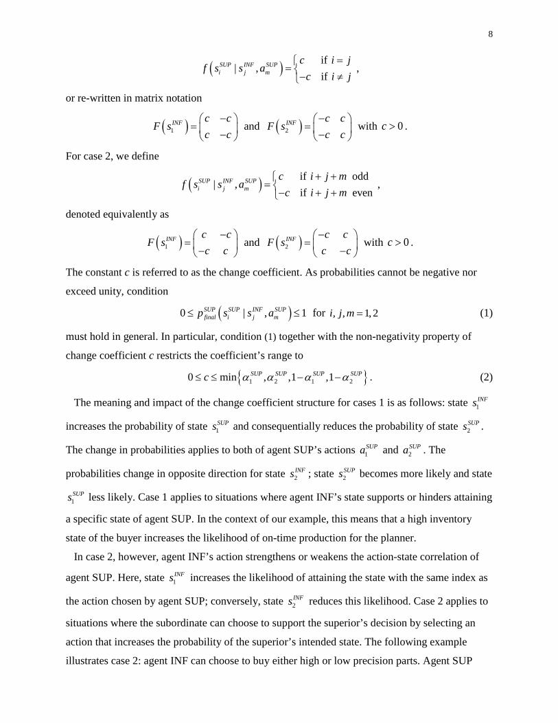
We choose the influence function to be a constant and consider two cases throughout this paper.

For case 1, the influence function is

8

( ) if| ,

ifSUP INF SUPi j m

c i jf s s a

c i j=

= − ≠ ,

or re-written in matrix notation

( )1INF c c

F sc c

− = −

and ( )2INF c c

F sc c

− = −

with 0c > .

For case 2, we define

( ) if odd| ,

if evenSUP INF SUPi j m

c i j mf s s a

c i j m+ +

= − + + ,

denoted equivalently as

( )1INF c c

F sc c

− = −

and ( )2INF c c

F sc c−

= − with 0c > .

The constant c is referred to as the change coefficient. As probabilities cannot be negative nor

exceed unity, condition

( )0 | , 1SUP SUP INF SUPfinal i j mp s s a≤ ≤ for , , 1, 2i j m = (1)

must hold in general. In particular, condition (1) together with the non-negativity property of

change coefficient c restricts the coefficient’s range to

{ }1 2 1 20 min , ,1 ,1SUP SUP SUP SUPc α α α α≤ ≤ − − . (2)

The meaning and impact of the change coefficient structure for cases 1 is as follows: state 1INFs

increases the probability of state 1SUPs and consequentially reduces the probability of state 2

SUPs .

The change in probabilities applies to both of agent SUP’s actions 1SUPa and 2

SUPa . The

probabilities change in opposite direction for state 2INFs ; state 2

SUPs becomes more likely and state

1SUPs less likely. Case 1 applies to situations where agent INF’s state supports or hinders attaining

a specific state of agent SUP. In the context of our example, this means that a high inventory

state of the buyer increases the likelihood of on-time production for the planner.

In case 2, however, agent INF’s action strengthens or weakens the action-state correlation of

agent SUP. Here, state 1INFs increases the likelihood of attaining the state with the same index as

the action chosen by agent SUP; conversely, state 2INFs reduces this likelihood. Case 2 applies to

situations where the subordinate can choose to support the superior’s decision by selecting an

action that increases the probability of the superior’s intended state. The following example

illustrates case 2: agent INF can choose to buy either high or low precision parts. Agent SUP

9

uses these parts as input to its production process and can set the machine setting to either ‘high

quality’ or ‘high speed,’ whichever its customer prefers. The high precision parts enable agent

SUP to better control the production process and achieve the desired state, whereas the low

precision parts make the link between agent SUP’s decision and the outcome less pronounced.

Finally, we discuss the mathematical description of the reward influence. The reward for agent

INF is affected by agent SUP’s state dependent reward, of which agent INF receives a

proportional share b that is referred to as the share coefficient. The final reward for agent INF is

( ) ( ) ( ),INF INF SUP INF INF INF SUP SUP INF SUPfinal final i j j i j ir r s s r s b r s bρ ρ= = + ⋅ = + ⋅ with , 1, 2i j = .

Agent SUP’s reward

( )SUP SUP SUP SUPi ir r s ρ= = with 1, 2i =

is unaffected. As the initial reward of agent SUP is identical to its final reward, we abstain from

using the subscript ‘final’ here.

The following assumptions are made in order to create an interesting agent interaction that

requires the agents to reason about a non-trivial decision strategy:

1 2SUP SUPρ ρ> and 1 2

INF INFρ ρ< (3)

and also, without loss of generality

1,2

SUP INFm nα α > for , 1, 2m n = . (4)

Inequalities in (3) express that agent SUP prefers state 1SUPs over 2

SUPs and agent INF reversely

prefers 2INFs over 1

INFs , at least initially. Expression (4) states that an action is linked to the state

with the same index; in other words, there is a corresponding action for every state, which is the

most likely consequence of the respective action. This restriction circumvents redundant cases in

the analysis, but does not limit the generality of the model. Table 1 provides an overview of the

notation.

Table 1: Overview of notation SUPma , INF

na actions SUPis , INF

js states

( )SUP SUPir s

reward function unaffected by interaction

( )INF INFjr s , ( ),INF SUP INF

final i jr s s reward function before, after interaction SUPR , INFR reward matrices (before interaction) SUPiρ , INF

jρ rewards (before interaction)

10

( )|INF INF INFj np s a trans. prob. function unaffected by interaction

( )|SUP SUP SUPi mp s a , ( )| ,SUP SUP INF SUP

final i j mp s s a trans. prob. function before, after interaction SUPP , INFP transition probability matrices (before interaction) SUPmα , INF

nα transition probabilities (before interaction)

( )| ,SUP INF SUPi j mf s s a influence function

( )INFjF s influence matrix

c change coefficient

b share coefficient Both agents are faced with a decision for which they should take into account the other agent’s

influence on reward and transition matrices. The details of the agent interaction are graphically

summarized in Figure 1. Based on the concept of dependency graphs (Dolgov and Durfee, 2004),

a solid arrow indicates an influence on transition probabilities and a dashed arrow represents a

reward influence.

SUP

INF

1SUPa

2SUPa

( )| ,SUP SUP INF SUPfinal i j mp s s a

1INFa

2INFa

( )|INF INF INFj np s a

1SUPs

2SUPs

1INFs

2INFs

Influenceon transition probability

Influenceon reward

Figure 1: Graphical representation of agent interaction

The agent interaction represents a game-theoretic situation that is analyzed in the following

section.

3.3. Analysis: Agent Interaction and Optimal Decision-Making

We assume that agents are risk-neutral and rational, i.e. agents maximize their expected

utilities, or equivalently their expected rewards. The risk-neutrality assumption can be relaxed by

introducing a concave utility function – at the cost of losing, or at least complicating, closed-

form solution results. Furthermore, the rationality assumption can be relaxed to a bounded

11

rationality assumption (Simon, 1979). For this extension of the model, the analytic solutions are

determined and given to the agents by a trustworthy (and rational) source such that the

computational effort for each (boundedly rational) agent is reduced to basic arithmetic

operations.

As information asymmetry is commonplace in organizations, we assume that agents have only

private information and need to communicate with other agents to elicit their information. We

assume that the organization has mechanisms in place (oversight, fines) that force agents to

truthfully report their private information. Without this assumption, agents would have

incentives to misrepresent their private information. Given the relevant and correct data, rational

agents are able to calculate both their own and the other party’s expected rewards, and thus can

decide which decisions yield the highest expected rewards for themselves. Hence, agents will

engage in a game-theoretic reasoning process, recognizing the dependency of each other’s

decisions. The expected reward for agent INF is calculated as follows:

( ) ( ) ( ) ( )2 2

1 1| , , | | ,INF SUP INF INF SUP INF INF INF INF SUP SUP INF SUP

final m n final i j j n final i j mi j

E r a a r s s p s a p s s a= =

= ⋅ ⋅∑∑ . (5)

The expected reward for agent SUP is calculated similarly:

( ) ( ) ( ) ( )2 2

1 1| , | | ,SUP SUP INF SUP SUP INF INF INF SUP SUP INF SUP

m n i j n final i j mi j

E r a a r s p s a p s s a= =

= ⋅ ⋅∑∑ . (6)

The expected rewards of both agents are the entries of a game matrix in normal form as shown in

Figure 2. The game matrix serves as the basis for the agents’ decision-making process. A

symbolic representation of the game matrix is introduced here for its use in figures thereafter.

1INFa 2

INFa

1SUPa ( ) ( )1 1 1 1| , , | ,SUP SUP INF INF SUP INF

finalE r a a E r a a ( ) ( )1 2 1 2| , , | ,SUP SUP INF INF SUP INFfinalE r a a E r a a

2SUPa ( ) ( )2 1 2 1| , , | ,SUP SUP INF INF SUP INF

finalE r a a E r a a ( ) ( )2 2 2 2| , , | ,SUP SUP INF INF SUP INFfinalE r a a E r a a

Agent INF

Age

nt S

UP

Symbolic representation

Figure 2: Game matrix in normal form

Different values of share coefficient b and change coefficient c can lead to different decision

strategies. We assume that the coefficients have already been chosen by the organizational

designer and have been communicated to the agents, the details of which are discussed later in

this section.

12

Furthermore, the type of influence function (case 1 or 2) also affects the agents’ decision

strategies. We investigate both cases in our analysis and begin with case 1.

3.3.1. Case 1

Figure 3 illustrates which action by which agent can be expected for given values of c and b.

We derive Nash equilibria in dominant strategies, which are represented through pictorial game

matrices as defined in Figure 2. Note that due to the given data in Figure 3 and property (2)

0 0.4c≤ ≤ must hold.

0 0.05 0.1 0.15 0.2 0.25 0.3 0.35 0.40

0.05

0.1

0.15

0.2

0.25

0.3

change coefficient c

shar

e co

effic

ient

b

Area 1

Phase transition

Area 2

Legend:

Nash-equilibriumHighest expected rewardfor agent SUP or INF

Data:

405

SUPR =

0.6 0.40.45 0.55

SUPP =

21

INFR−

= −

0.65 0.350.1 0.9

INFP =

Figure 3: Phase diagram with reward matrices, case 1

One can distinguish between two areas in this b-c diagram, leading to different equilibrium

outcomes. In area 1, the Nash equilibrium, which predicts the agent behavior, is an unfavorable

outcome for agent SUP. The star symbol in the upper left corner of the game matrix indicates the

best possible outcome for agent SUP, which does not coincide with the Nash equilibrium that is

represented by the oval in the upper right matrix cell. In area 2, however, the Nash equilibrium

provides the best possible outcome for both agents.

The transition line, which is the divider between both areas, indicates when it is advantageous

for agent INF to switch from strategy 2INFa to 1

INFa . The functional relationship of the transition

line is derived as follows:

( ) ( )1 1 1 2| , | ,INF SUP INF INF SUP INFfinal finalE r a a E r a a≥

( ) ( ) ( ) ( ) ( )1 1 1 1 2 1 1 11INF SUP INF SUP INF SUP INF SUPb c b cρ ρ α α ρ ρ α α+ ⋅ ⋅ + + + ⋅ − ⋅ −

13

( ) ( ) ( ) ( ) ( )1 2 1 1 2 2 1 21 1 1INF SUP INF SUP INF SUP INF SUPb c b cρ ρ α α ρ ρ α α+ + ⋅ ⋅ − − + + ⋅ − ⋅ − +

( ) ( ) ( ) ( ) ( )1 1 2 1 2 1 2 11INF SUP INF SUP INF SUP INF SUPb c b cρ ρ α α ρ ρ α α≥ + ⋅ − ⋅ + + + ⋅ ⋅ −

( ) ( ) ( ) ( ) ( )1 2 2 1 2 2 2 11 1 1INF SUP INF SUP INF SUP INF SUPb c b cρ ρ α α ρ ρ α α+ + ⋅ − ⋅ − − + + ⋅ ⋅ − +

( )

2 1

1 22

INF INF

SUP SUPb

cρ ρρ ρ

−≥

− (7)

Note that transition function (7) does not depend on agent INF’s or agent SUP’s transition

probabilities. We assume that on the transition line, where agent INF is indifferent, agent INF

chooses the action that is beneficial to agent SUP (i.e., action 1INFa ). For agent SUP, such a

transition line does not exist because its dominant strategy is always to choose 1SUPa .

Next, we address the question of organizational design, i.e. which values of share coefficient b

and change coefficient c an organizational designer chooses. We assume that the designer’s

primary interest is to enable both agents to attain their highest possible expected rewards

followed by the secondary goal of minimizing cost. In a real-world application, such a primary

and secondary goal can be found in situations where the costs are small compared to the gains in

coordination benefits. This goal hierarchy is particularly plausible, when costs (e.g. the reward

share) are paid by the customer, or come from another source outside the organization. The

designer is interested in the well-being of the organization and agents’ rewards – especially with

external reward contributions – are a direct measure of the organization’s performance. For the

following analysis, we do not need to specify a concrete cost function ( ),C b c as it suffices to

assume that the designer’s cost function increases for both coefficients c and b.

With change coefficient c the designer chooses how strongly a superior agent depends on the

performance of its subordinate agent. In the context or our example, change coefficient c is a

measure for the spread between agent INF’s order options. A larger c results in two more

divergent order options and, consequentially, agent SUP is more dependent on agent INF’s

choice.

Returning to the analysis, we conclude that area 2 is preferred over area 1 due to the designer’s

primary objective. Following its secondary goal, the designer’s cost minimal choice within area

2 is on the transition line. The transition line represents a Pareto-efficient frontier along which

the optimal point ( ),b c∗ ∗ is located. The actual cost structure determines the exact allocation

and, for most cost functions, the solution will be unique. See Wernz and Deshmukh (2007b) for

an actual calculation with a concrete objective and cost function.

14

In a final step, we address aspects of communication and privacy. To determine the Pareto-

efficient values of c and b, the designer needs to elicit only aggregated reward information from

both agents (i.e., 1 2SUP SUPρ ρ− and 2 1

INF INFρ ρ− ). Once the designer’s choice of the organizational

coefficients is communicated to both agents, they merely need to exchange their aggregate

reward information. Alternatively, this information could be provided by the designer. These

results indicate that only little information and communication is necessary, and agents do not

have to reveal much of their private information.

3.3.2. Case 2

The influence function of case 2 generates more than one transition function, which leads to a

more complex phase diagram. Furthermore, two sub-cases emerge based on the relationship

between 1INFα and 2

INFα . In this section, we discuss the sub-case for 1 2INF INFα α< . The

complementing sub-case 1 2INF INFα α> leads to a comparable phase diagram which is not

discussed in this paper; see Wernz and Deshmukh (2007a) for the complementing sub-case.

As a reminder, transition lines divide the b-c diagram into different regions from which

equilibrium phases are derived. The areas and the corresponding pictorial reward matrices are

shown in Figure 4 and based on the same data as case 1.

0 0.05 0.1 0.15 0.2 0.25 0.3 0.35 0.40

0.05

0.1

0.15

0.2

0.25

0.3

change coefficient c

shar

e co

effic

ient

b

Area 1

Area 2a

Area 4

Area 2b

Area 3

Area 5b

Area 5a

Figure 4: Phase diagram with reward matrices, case 2

In area 1, the Nash equilibrium is attained for the action pair ( )1 2,SUP INFa a . This Nash

equilibrium and all subsequent equilibria discussed in this section are Pareto-efficient unless

15

otherwise stated. In area 1, the Nash equilibrium is identical to the “no influence case” 0b c= =

because the influence of the agents on each other is not strong. Agent SUP does not receive its

highest possible expected reward that would be attained at ( )1 1,SUP INFa a . In order to motivate

agent INF to change its strategy to 1INFa given 1

SUPa , the share coefficient b must exceed the

threshold determined by transition function .

The game-theoretic situation in area 4 is similar to area 1; in area 4, the Nash equilibrium is at

( )2 2,SUP INFa a , but does not lead to the highest possible reward for both agents. In area 2a,

however, both agents reach the Nash equilibrium by choosing ( )1 1,SUP INFa a and both receive the

highest possible expected rewards. For area 2b, a second Nash equilibrium at ( )2 2,SUP INFa a

emerges, however it is Pareto-dominated by ( )1 1,SUP INFa a . The optimal strategy for areas 2a and

2b is the same, which is recognized by the fact that the combined area is referred to as area 2,

with sub-areas 2a and 2b graphically separated by a dashed line. There are two Nash equilibria in

area 3. Strategy pair ( )1 1,SUP INFa a is favored by agent SUP and ( )2 2,SUP INFa a is preferred by agent

INF. This constellation is a well-known dilemma in game theory, referred to as ‘battle of the

sexes’ (Fudenberg and Tirole, 1991).

Area 5 is attained for 0.3c > and the strategy pair ( )2 2,SUP INFa a is a Nash equilibrium with the

highest expected rewards for both agents. Similarly to area 2, one can distinguish between two

sub-regions. Area 5a has one Nash equilibrium and area 5b has a second Nash equilibrium that is

Pareto-dominated by strategy ( )2 2,SUP INFa a .

The results of the analysis, visualized in the phase diagram, enable the organizational designer

to identify the optimal choices for coefficients c and b. Areas 2 and 5 satisfy the designer’s

primary objective. The exact allocation along a Pareto-efficient frontier is determined by the

secondary goal.

Similar to (7), we derived the transition functions, which are presented in the following table.

16

Table 2: Results

# transition functions reward transitions

0c ≥ ( ) ( )1 1 1 2| , | ,SUP SUP INF SUP SUP INF

final finalE r a a E r a a≥

( ) ( )2 2 2 1| , | ,SUP SUP INF SUP SUP INFfinal finalE r a a E r a a≥

0b ≥ (and c smaller than transition function )

( ) ( )1 1 2 1| , | ,INF SUP INF INF SUP INFfinal finalE r a a E r a a≥

( ) ( )1 2 2 2| , | ,INF SUP INF INF SUP INFfinal finalE r a a E r a a≥

( )1 2

2

12 2 1

SUP SUP

INFc α α

α+ −

≥−

( ) ( )2 2 1 2| , | ,SUP SUP INF SUP SUP INF

final finalE r a a E r a a≥

( ) ( )2 2 1 2| , | ,INF SUP INF INF SUP INFfinal finalE r a a E r a a≥

( )2 1

1 22

INF INF

SUP SUPb

cρ ρρ ρ

−≥

− ( ) ( )1 1 1 2| , | ,INF SUP INF INF SUP INF

final finalE r a a E r a a≥

( )( )

( )( ) ( )

2 1 1 2

1 2 1 2 2 1

1

1 2

INF INF INF INF

SUP SUP SUP SUP INF INFb

c

ρ ρ α α

ρ ρ α α α α

− + −≥ ⋅

− + − − − ( ) ( )1 1 2 2| , | ,INF SUP INF INF SUP INF

final finalE r a a E r a a≥

( )1 2

2 1

12

SUP SUP

INF INFc α α

α α+ −

≥−

( ) ( )2 2 1 1| , | ,SUP SUP INF SUP SUP INFfinal finalE r a a E r a a≥

Again, we address aspects of communication and privacy. For area 5, the organizational

designer determines the change coefficient c associated with transition line and sets 0b = .

Thus, the designer acquires aggregated information on the agents’ transition probabilities,

1 2SUP SUPα α+ and 2 1

INF INFα α− , respectively. For area 2 the designer considers a value pair ( ),b c

on transition line that is left of transition line . The designer elicits the following

information from both agents: 1 2SUP SUPα α+ , 2

INFα , 1 2SUP SUPρ ρ− and 2 1

INF INFρ ρ− . Conclusively,

determining the optimal values for coefficients c and b in area 2 requires more communication

and revelation of private information compared to area 5.

4. Horizontal Extension

The two-agent model of Section 3 is generalized to n+1 agents. We consider one supremal

agent that interacts with n infimal agents. In the context of our example from Section 3.1, the n

infimal agents could be n buyers that, independently of each other, order similar raw material

inputs. One can find such a scenario in organizations that rely on a multiple-source strategy for

raw material.

For the mathematical description, coefficients and parameters get augmented with an

additional index 1,...,i n= corresponding to the different agents INFi. The transition probability

of agent SUP becomes

17

( ) ( ) ( )( ) ( ) ( )( )11

1| ,..., ,..., , | | ,

nSUP SUP INF INFi INFn SUP SUP SUP SUP SUP INFi SUPfinal j m j m i j mi n i

ip s s s s a p s a f s s aν ν ν ν

=

= +∑

with , 1, 2j m = and state index function ( ) 1,2iν = .

The two different influence functions, cases 1 and 2 from the previous sections, continue to

exhibit different behavior. We begin our analysis with case 1.

4.1. Case 1: Independent Infimal Agents

For this type of influence function, we will show that, given appropriate choices for share and

influence coefficients ib and ic , each agent INFi’s best response is to choose strategy 1INFia

regardless of the actions taken by any other infimal agents. Thereby, all n+1 agents can reach the

Nash equilibrium with the highest possible expected rewards for all agents. The details are

presented in the following theorem and proof.

Theorem 4.1: The incentive level to motivate agent INFi to choose action 1INFia over initially

preferred action 2INFia is

( )

2 1

1 22

INFi INFi

i SUP SUPi

bcρ ρρ ρ

−≥

− for 1,...,i n= . (8)

Proof: We evaluate a three-agent situation by solving

( )( ) ( )( )1 1 2 1 1 21 1 1 22 2| , , | , ,INF SUP INF INF INF SUP INF INF

final finalE r a a a E r a a aµ µ≥

with action index function ( )2 1, 2µ = , which gives

( )

1 12 1

11 1 22

INF INF

SUP SUPb

cρ ρρ ρ

−≥

−. (9)

Transition function (9) is identical to the two-agent result in (7). The decision and

parameters/coefficients of agent INF2 have no influence on agent INF1’s transition function.

Since the interaction of agent INF1 and INF2 with agent SUP are structurally identical, transition

function (9) also applies to agent INF2, with corresponding indices. Furthermore, adding

additional infimal agents has no effect on an infimal agent’s transition function. The transition

functions for the two- and three-agent model are identical. Thus, we can conclude that (9) can be

generalized to n+1 agents. Solving

( ) ( )( ) ( ) ( )( )1 11 1 1 21 1| , ,..., ,..., | , ,..., ,...,INFi SUP INF INFi INFn INFi SUP INF INFi INFn

final finaln nE r a a a a E r a a a aµ µ µ µ≥

results in

18

( )

2 1

1 22

INFi INFi

i SUP SUPi

bcρ ρρ ρ

−≥

− for 1,...,i n= . (10) □

Agents INFi can determine their optimal decision strategies without knowing data or decisions

of the other agents on the same hierarchical level. The decisions of the other infimal agents affect

all agents’ expected rewards, but those decisions do not influence any infimal agent’s optimal

decision strategy.

In summary, the problem of multiple infimal agents in case 1 decomposes for each infimal

agent. This decomposition results in low communication and information exchange needs

between the agents. Each agent INFi has to elicit only the reward difference 1 2SUP SUPρ ρ− from

agent SUP and the share and change coefficients ib and ic from the organizational designer to

determine its optimal strategy.

4.2. Case 2: Interdependent Infimal Agents

For the second type of influence function, we find that ic and ib depend on the other infimal

agents. Thus, infimal agents are no longer independent from one another.

Similar to the derivation of transition function in the one infimal agent case, we evaluate

( ) ( )1 11 1 1 1 2 2 2 2| , ,..., ,..., | , ,..., ,...,INFi SUP INF INFi INFn INFi SUP INF INFi INFn

final finalE r a a a a E r a a a a≥

which gives

( )

2 1 1 2

1 21 2 1 2

1

1

1 2

INFi INFi INFi INFi

i nSUP SUPSUP SUP INFj INFj

jj

bc

ρ ρ α αρ ρ α α α α

=

− + −≥ ⋅

− + − + −∑. (11)

The denominator in inequality (11) depends on all infimal agents, which means that the infimal

agents are no longer independent in their decision-making process. The n-infimal agent versions

of transition functions and also exhibit dependency results. Only the n-infimal agent

version of transition function shows decision independence between infimal agents and

inequality (8) applies to this case as well.

In summary, Section 4 extends the two-agent interaction to n+1 agents. We determined under

which circumstances infimal agents are independent from one another when making a decision,

and when not. The independence between infimal agents can be contributed to transition

functions of type . Case 1, studied in the beginning of this section, has only a type transition

function and the problem therefore decomposes for each infimal agent. For case 2, the equations

of other transition functions document an influence of infimal agents on one another. All infimal

agents have to elicit information from each other to determine their optimal decisions.

19

5. Vertical Extension

In a next step, the agent interaction model is extended in the vertical direction to allow for a

chain of supremal and infimal agents. In the context of our example, an agent that is higher in the

chain, and thus superior to the planner, could be a production manager overseeing multiple

products. Moving upwards in the hierarchical chain, the next higher level agent could be an

operations manager, preceded by the vice-president of operations and finally the CEO of the

organization. Hierarchically below the buyer could be a material handler that influences the

performance of the buyer, and so on.

We refer to the m agents that form the hierarchical chain as agents Ak, with 1,...,k m= . Except

for the agent at the top or bottom of the chain, agents take on the role of both subordinates and

superiors as they are interacting in both directions in the hierarchy.

The reward situation of the two agents at the top of the hierarchy, agent A1 and A2, is identical

to the two-agent interaction in Section 3. The next lower level agent, agent A3, receives an

incentive payment based on agent A2’s final reward, which includes the incentive payment based

on agent A1’s performance. For a general m agent situation, this reward mechanism continues

down the chain, so that even the reward of the agent at the very bottom of the chain is influenced

by the reward of the agent at the top.

For the probability influence, the situation of the two agents at the bottom of the chain, agent

Am and A(m-1), is identical to the two-agent interaction. The transition probability of the next

higher level agent, agent A(m-2), is directly affected by agent A(m-1), but also indirectly through

Am. The general mathematical formulation of both rewards and transition probabilities can be

found in the Appendix.

The choice of influence structure affects, as before, the agent behavior. For the following

analyses of cases 1 and 2, we assume that the top most agent A1 prefers 11As over 1

2As and all

other agents prefer 2Aks over 1

Aks .

5.1. Case 1: Optimal Decisions with Aggregated and Local Information

For the influence functions kf of case 1, we find that agents in a hierarchical chain have only

to communicate locally (i.e., with their immediate supremal agent) to determine their optimal

course of action. The details are presented in the following theorem and proof.

Theorem 5.1: The optimal incentive level to motivate agent A(k+1) to choose action ( )11A ka +

over initially preferred action ( )12A ka + is

20

( ) ( )

( )1 1

2 1

2 1

A k A k

k Ak Akk

bcρ ρ

ρ ρ

+ +−=

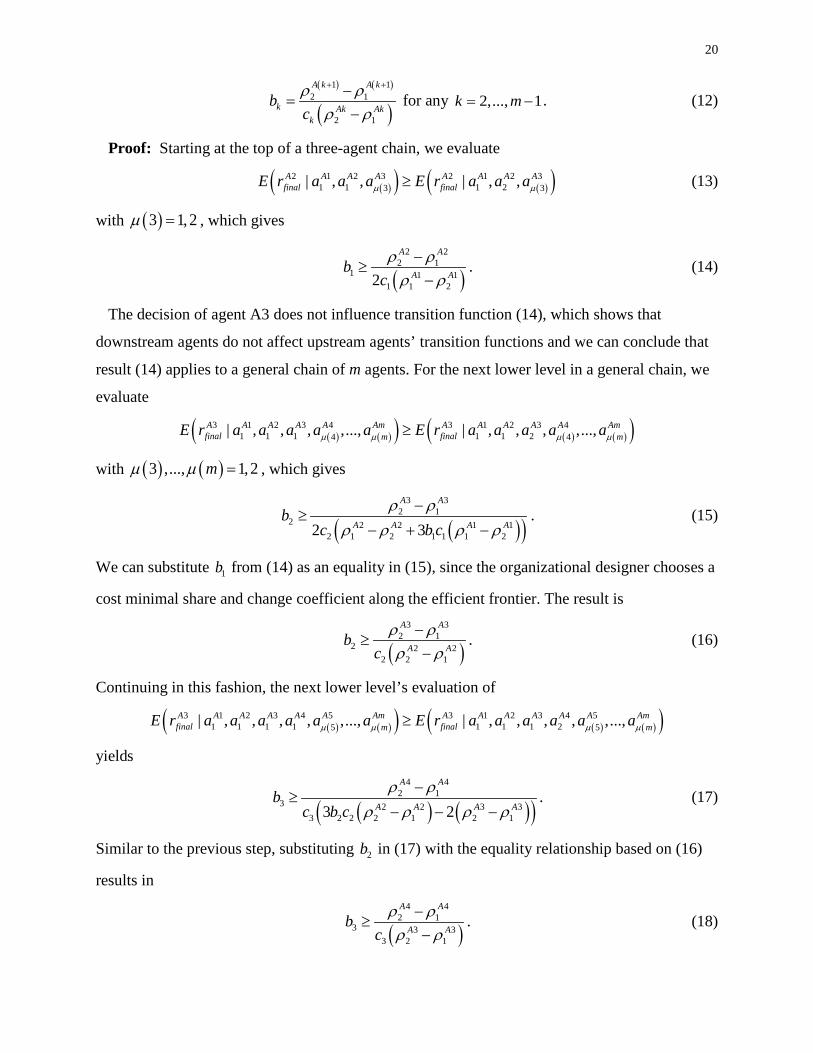
− for any 2,..., 1k m= − . (12)

Proof: Starting at the top of a three-agent chain, we evaluate

( )( ) ( )( )2 1 2 3 2 1 2 31 1 1 23 3| , , | , ,A A A A A A A A

final finalE r a a a E r a a aµ µ≥ (13)

with ( )3 1,2µ = , which gives

( )

2 22 1

1 1 11 1 22

A A

A Ab

cρ ρρ ρ−

≥−

. (14)

The decision of agent A3 does not influence transition function (14), which shows that

downstream agents do not affect upstream agents’ transition functions and we can conclude that

result (14) applies to a general chain of m agents. For the next lower level in a general chain, we

evaluate

( ) ( )( ) ( ) ( )( )3 1 2 3 4 3 1 2 3 41 1 1 1 1 24 4| , , , ,..., | , , , ,...,A A A A A Am A A A A A Am

final finalm mE r a a a a a E r a a a a aµ µ µ µ≥

with ( ) ( )3 ,..., 1, 2mµ µ = , which gives

( )( )

3 32 1

2 2 2 1 12 1 2 1 1 1 22 3

A A

A A A Ab

c b cρ ρ

ρ ρ ρ ρ−

≥− + −

. (15)

We can substitute 1b from (14) as an equality in (15), since the organizational designer chooses a

cost minimal share and change coefficient along the efficient frontier. The result is

( )

3 32 1

2 2 22 2 1

A A

A Ab

cρ ρρ ρ

−≥

−. (16)

Continuing in this fashion, the next lower level’s evaluation of

( ) ( )( ) ( ) ( )( )3 1 2 3 4 5 3 1 2 3 4 51 1 1 1 1 1 1 25 5| , , , , ,..., | , , , , ,...,A A A A A A Am A A A A A A Am

final finalm mE r a a a a a a E r a a a a a aµ µ µ µ≥

yields

( ) ( )( )

4 42 1

3 2 2 3 33 2 2 2 1 2 13 2

A A

A A A Ab

c b cρ ρ

ρ ρ ρ ρ−

≥− − −

. (17)

Similar to the previous step, substituting 2b in (17) with the equality relationship based on (16)

results in

( )

4 42 1

3 3 33 2 1

A A

A Ab

cρ ρρ ρ

−≥

−. (18)

21

Transition function (18) is structurally identical to (16). The decision situation in both cases is

also identical. Agents A3 and A4 both have supremal agents and have been motivated to choose

actions 1a over the initially preferred actions 2a . The results from (16) and (18) repeat for

agents further down the chain. Due to the similarity and repetition of the agents’ situation

throughout the chain, we can conclude that in general

( ) ( )( )( )

( )( ) ( ) ( )( )1 1 2 1 111 1 1 22| ,..., , , ,..., | ... ...A k A k A k A k A kA Ak Am

final finalk mE r a a a a a E r aµ µ+ + + + +

+ ≥

results in

( ) ( )

( )1 1

2 1

2 1

A k A k

k Ak Akk

bcρ ρ

ρ ρ

+ +−≥

− for all 2,...,k m= . (19) □

This result can be interpreted as follows: given the assumption of optimal behavior of the

organizational designer and higher level agents, agent A(k+1) can determine its optimal behavior

by knowing only its own private information and the aggregate reward information of agent Ak.

Thereby, chain-wide optimal and beneficial behavior is possible with local interaction and

information. The organizational designer has the ability to create influence and incentive

structures that lead to cooperative actions by all agents.

5.2. Case 2: Optimal Decisions with Comprehensive and Global Information

For the influence function of case 2, the results are very different. In Section 4, we saw that the

transition function had the same properties in both cases. This result, however, is no longer

valid for a hierarchical chain of agents under case 2. For a chain with three agents, we evaluate

for agent A2

( ) ( )2 1 2 3 2 1 2 31 1 1 1 2 1| , , | , ,A A A A A A A A

final finalE r a a a E r a a a≥

which gives

( ) ( )( )( ) ( )( )

2 2 2 2 32 1 1 2 2 1

1 1 1 2 2 31 1 2 1 2 2 1

1 2 1 2

2 1 3 1 2

A A A A A

A A A A A

cb

c c

ρ ρ α α α

ρ ρ α α α

− + − − −≥

− + − − −. (20)

This result is significantly more complex than the previous result (14). No repetitive structure

emerges when moving down the hierarchical chain. The other types of transition functions

considered in earlier sections also give complex results, or do not even exist.

In conclusion, when using influence functions of case 2, a compact result for a general

hierarchical chain of m agents with little information needs for the agents does not exist. Each

agent constellation grows in complexity with the number of agents considered, and each

structure needs to be analyzed individually.

22

Taking the results of cases 1 and 2 for the horizontal and vertical extension together, we

conclude: coordination of decisions between agents is easier when infimal agents can make a

particular outcome for their supremal agent more/less attainable (case 1) compared to when

infimal agents can make actions for their supremal agent more/less powerful (case 2).

6. Arborescent Decision Networks

The findings from the vertical and horizontal generalization of Sections 4 and 5 can be

combined to a general arborescent decision network model, i.e. a model for a tree-structured

organization with multiple levels and multiple agents on each level. This model represents the

multiscale decision-making model we set out to derive. Each agent can determine its optimal

decision that takes the effects across all organizational scales into account.

For case 1, the transition functions that have been derived continue to apply and are not

affected by the combination of the vertical and horizontal generalization. As agents on the same

hierarchical level do not influence each others’ decisions, they certainly do not influence other

agents further up or down in the hierarchy. For case 2, a compact solution cannot be derived due

to interdependency (horizontal extension) and lack of extendibility (vertical extension).

For case 1, we will illustrate the model’s capability to bridge the organizational scales of

distributed decision-makers in a hierarchical organization through an example. Before that, we

have to extend our current notation to allow for unambiguous references to all agents in the

network. The vertical level is indexed by k, with 1,...,k m= , and the horizontal level by i, with

1,...,i n= , as before. Agents are labeled as shown in Figure 5. Supremal-infimal relationships are

represented by a connecting line, as customary in organizational charts.

1,1

2,2(1)

3,5(2)3,4(2)

2,1(1)

3,2(1)3,1(1) 3,3(1)

Figure 5: Organizational chart and notation

The notation to reference agents is k,i(i’), where i’ is the horizontal index of the agent superior

to agent i. The top most agent 1,1 has no supremal agent above itself, and thus no parentheses are

23

used. Agents on the second level ( 2k = ) have only one possible supremal agent, which is agent

1,1. The notation of the supremal agent is redundant in this case, yet included for consistency.

On the third vertical level, the reference to the superior agent becomes necessary to

unambiguously indicate supremal-infimal agent relationships. For example, agent 3,2(1) is

subordinate to agent 2,1(1) and agent 3,4(2) is subordinate to agent 2,2(1). Bold font indicates

the corresponding value pairs.

Share coefficients are indexed by k,i[i’’], where i’’ is the horizontal index of the subordinate

agent receiving the reward share. The same index notation is used for the change coefficients.

For rewards ρ , we leave out the parenthesis in the index for a more compact notation and use

only k,i.

An example of an agent interaction for the tree-structured network defined in Figure 5 is

analyzed in the following paragraphs. We determine the transition functions, which entail the

agents’ choices given their associated reward shares. We continue to assume optimal choices of

the agents and organizational designer. The example has the following properties. Agent 1,1

prefers state 1,11s over 1,1

2s , as we have assumed throughout this paper. Agent 2,2(1) also prefers

its first state 2,21s over the second state 2,2

2s . All other agents initially prefer state 2s over 1s .

For the following values of share coefficients b, all agents will (weakly) prefer action 1a over

2a . These are also the values which the organizational designer chooses from:

( )

2,1 2,12 1

1,1[1] 1,1 1,11,1[1] 1 22

bcρ ρ

ρ ρ−

=−

(21)

1,1[2] 0b = (22)

( )3, 3,2 1

2,1[ ] 2,1 2,12,1[ ] 2 1

i i

ii

bc

ρ ρρ ρ−

=−

for 1, 2,3i = (23)

( )3, 3,2 1

2,2[ ] 2,2 2,22,2[ ] 1 22

i i

ii

bc

ρ ρρ ρ−

=−

for 4,5i = . (24)

The example covers all possible pairwise combinations of agents’ preferences. Equation (22)

applies to two hierarchically interacting agents that prefer 1s over 2s . No incentive payment is

needed to align their interests. Equations (21) and (24) apply to the scenario where the supremal

agent prefers 1s over 2s , and the infimal agent 2s over 1s . This scenario coincides with the two-

24

agent interaction model of Section 3. Finally, equation (23) applies to two agents that prefer 2s

over 1s .

7. Conclusion

Our model represents the decision-making situations of agents in large hierarchical

organizations. A multiscale decision-making framework is able to bridge organizational scales

between decision-makers and provides compact analytic, closed-form solutions. The effects of

decisions made at the top of the organization can be taken into account when making decisions at

the bottom and vice versa. Individual decision-makers can use the model to determine the best

course of action and identify information needs for optimal decision-making. The organizational

design can be chosen to motivate cooperative behavior among self-interested agents and to align

agents’ goals with the interests of the organization.

A two-agent model that formalizes the hierarchical agent interaction serves as an initial

building block. We investigate two types of influence functions (cases 1 and 2) that lead to

different results in agent behavior and information requirements for optimal decision-making.

The ensuing horizontal extension, in which one supremal agent interacts with many infimal

agents, continues to show differences for the two cases considered. In case 1, infimal agents are

independent from one another when choosing the best course of action, whereas in case 2,

infimal agents are interdependent. The following vertical extension investigates a hierarchical

chain of agents in superior-subordinate relationships. In case 1 of the vertical extension, agents

have only to acquire a small amount of data from their superior and, with optimal behavior of the

upstream agents and organizational designer, can make an optimal decision. For case 2, chain-

wide information exchange is necessary.

In a final step, we merge the horizontal and vertical extension to a multi-agent hierarchical

interaction model. All agents influence each other’s expected rewards, but for the influence

function of type 1, local information exchange with a straightforward decision rule is sufficient

to determine the best course of action for each individual decision-maker. This property makes

the proposed multiscale decision-making model attractive for real-world decision-making where

data is scarce and/or uncertain, communication is costly, and individuals are not boundlessly

rational and/or have to make decisions quickly with little computational effort.

25

Appendix

In Section 5, the reward function for any agent Ak can be mathematically expressed as

( ) ( )( )

( )( ) ( )( ) ( )1 1111 1, , ,A k A kAk Ak Ak A Ak Ak

final final k finalv k v k v v kr r s s s r s b r− −−−= = + ⋅

( )( ) ( )( )( )( ) ( )

( )( )( ) ( )( )1 1 2 2 1 1

1 1 2 1 2 11 2 1A k A k A k A kAk Ak A A

k k k k kv k v k v k vr s b r s b b r s b b b r s− − − −− − − − −− −= + ⋅ + ⋅ ⋅ + + ⋅ ⋅ ⋅ ⋅

( )( ) ( )( )11

1

kkAk Ak Ai Ai

jv k v ii j i

r s r s b−−

= =

= +

∑ ∏ (25)

with 1,2,..., 1k m= − and the state index function ( ) 1,2kν = . The share coefficient kb is the

percentage agent A(k+1) receives of agent Ak’s reward.

Similarly, the transition probability function can be stated in general terms. We begin with the

direct and indirect influence of the second to last agent A(m-2) resulting in the following final

transition probability

( ) ( ) ( ) ( ) ( )( )2 2 2 1 1| , , ,A m A m A m A m A m Amfinal i n o j lp s a a s s− − − − −

( ) ( ) ( )( ) ( ) ( ) ( )( ) ( ) ( )( )( )2 2 2 2 1 2 1 12 1| , | 1 , |A m A m A m m A m A m A m A mAm

i n m i j n m j l op s a f s s a f s s a− − − − − − − −− −= + ⋅ + ,

, , , , 1, 2i j l n o = . (26)

The influence function kf and change coefficient kc describes the effect of agent A(k+1) on the

transition probability of agent Ak. Multiplying all agents’ probabilities of reaching a particular

state with one another gives the overall probability p of reaching certain states given certain

actions:

( ) ( ) ( ) ( ) ( ) ( )( )1 2 1 21 2 1 2, , , , , ,A A Am A A Am

v v v m mp s s s a a aµ µ µ

( ) ( )( ) ( ) ( ) ( )( )( )

111

1

| , ,m m im

A jAk Ak Ak Aj Ajjv k k j j j

i kk j k

p s a f a s sµ µ ν ν

−−++

== =

= +

∑∏ ∏

( ) ( )( )1 1 11 1 2 1 2 11 1|A A A

mvp s a c c c c c cµ − = ± ± ± ± ⋅

( ) ( )( )2 2 22 2 3 2 3 12 2|A A A

mvp s a c c c c c cµ − ± ± ± ± ⋅ ⋅

( )( )( )

( )( )( ) ( ) ( )( )1 1 1

11 1| |A m A m A m Am Am Ammv m m v m mp s a c p s aµ µ

− − −−− −

± ⋅ (27)

with action index function ( ) 1, 2kµ = .

26

Acknowledgements

This research has been funded in part by NSF grants DMI-0122173, IIS-0325168 and

DMI-0330171.

References

Anandalingam, G. and V. Apprey, 1991. Multi-Level Programming and Conflict Resolution. European Journal of Operational Research 51 (2), 233-247.

Banks, J., C. Camerer and D. Porter, 1994. An Experimental Analysis of Nash Refinements in Signaling Games. Games and Economic Behavior 6 (1), 1–31.

Barber, K. S. 2007. Multi-Scale Behavioral Modeling and Analysis Promoting a Fundamental Understanding of Agent-Based System Design and Operation. Final Technical Report (AFRL-IF-RS-TR-2007-58). Retrieved Oct. 07, 2007, http://stinet.dtic.mil/cgi-bin/GetTRDoc?AD=ADA465613&Location=U2&doc=GetTRDoc.pdf.

Cho, I. K. and J. Sobel, 1990. Strategic Stability and Uniqueness in Signaling Games. Journal of Economic Theory 50 (2), 381-413.

Cruz Jr, J. B., M. A. Simaan, A. Gacic, H. Jiang, B. Letelliier, M. Li and Y. Liu, 2001. Game-Theoretic Modeling and Control of a Military Air Operation. IEEE Transactions on Aerospace and Electronic Systems 37 (4), 1393-1405.

Deng, X. and C. H. Papadimitriou, 1999. Decision-Making by Hierarchies of Discordant Agents. Mathematical Programming 86 (2), 417-431.

Dolbow, J., M. A. Khaleel and J. Mitchell, 2004. Multiscale Mathematics Initiative: A Roadmap. Technical report, Department of Energy, USA.

Dolgov, D. and E. Durfee, 2004. Graphical Models in Local, Asymmetric Multi-Agent Markov Decision Processes. Proceedings of the Third International Joint Conference on Autonomous Agents and Multiagent Systems-Volume 2, 956-963.

Fudenberg, D. and J. Tirole, 1991. Game Theory. MIT Press, Cambridge, MA. Geanakoplos, J. and P. Milgrom, 1991. A Theory of Hierarchies Based on Limited Managerial Attention. Journal of

the Japanese and International Economies 5 (3), 205-225. Gfrerer, H. and G. Zäpfel, 1995. Hierarchical Model for Production Planning in the Case of Uncertain Demand.

European Journal of Operational Research 86 (1), 142-161. Groves, T., 1973. Incentives in Teams. Econometrica 41 (4), 617-631. Hax, A. C. and H. C. Meal, 1975. Hierarchical Integration of Production Planning and Scheduling. Studies in the

Management Sciences, ed. M. A. Geisler, North Holland, Amsterdam. Heinrich, C. E. and C. Schneeweiss, 1986. Multi-Stage Lot-Sizing for General Production Systems. Multistage

Production Planning and Inventory Control. Lecture Notes in Economics and Mathematical Systems 266, eds. S. Axsäter, C. Schneeweiss and E. Silver, Springer, Berlin.

Krothapalli, N. K. C. and A. Deshmukh, 1999. Design of Negotiation Protocols for Multi-Agent Manufacturing Systems. International Journal of Production Research 37 (7), 1601-1624.

Laffont, J. J., 1990. Analysis of Hidden Gaming in a Three-Level Hierarchy. Journal of Law, Economics, & Organization 6 (2), 301-324.

Marschak, J. and R. Radner, 1972. Economic Theory of Teams. Yale University Press, New Haven.

27

Mesarovic, M. D., D. Macko and Y. Takahara, 1970. Theory of Hierarchical, Multilevel, Systems. Academic Press, New York.

Middelkoop, T. and A. Deshmukh, 1999. Caution! Agent Based Systems in Operation. InterJournal of Complex Systems 256.

Monostori, L., J. Váncza and S. Kumara, 2006. Agent-Based Systems for Manufacturing. CIRP Annals-Manufacturing Technology 55 (2), 697-720.

Nie, P., L. Chen and M. Fukushima, 2006. Dynamic Programming Approach to Discrete Time Dynamic Feedback Stackelberg Games with Independent and Dependent Followers. European Journal of Operational Research 169 (1), 310-328.

Özdamar, L., M. A. Bozyel and S. I. Birbil, 1998. A Hierarchical Decision Support System for Production Planning (with Case Study). European Journal of Operational Research 104 (3), 403-422.

Schneeweiss, C., 1995. Hierarchical Structures in Organizations: A Conceptual Framework. European Journal of Operational Research 86 (1), 4-31.

Schneeweiss, C., 2003a. Distributed Decision Making. Springer, Berlin. Schneeweiss, C., 2003b. Distributed Decision Making - A Unified Approach. European Journal of Operational

Research 150 (2), 237-252. Schneeweiss, C. and K. Zimmer, 2004. Hierarchical Coordination Mechanisms within the Supply Chain. European

Journal of Operational Research 153 (3), 687-703. Simon, H. A., 1979. Rational Decision Making in Business Organizations. The American Economic Review 69 (4),

493-513. Stackelberg, H. v., 1952. The Theory of the Market Economy. Oxford University Press, New York. Stadtler, H., 2005. Supply chain management and advanced planning––basics, overview and challenges. European

Journal of Operational Research 163 (3), 575-588. Vetschera, R., 2000. A Multi-Criteria Agency Model with Incomplete Preference Information. European Journal of

Operational Research 126 (1), 152-165. Weiss, G., 1999. Multiagent Systems: A Modern Approach to Distributed Artificial Intelligence. MIT Press,

Cambridge, MA. Wernz, C. and A. Deshmukh, 2007a. Decision Strategies and Design of Agent Interactions in Hierarchical

Manufacturing Systems. Journal of Manufacturing Systems 26 (2), 135-143. Wernz, C. and A. Deshmukh, 2007b. Managing Hierarchies in a Flat World. Proceedings of the 2007 Industrial

Engineering Research Conference, Nashville, TN, 1266-1271.