multiscale models for shapes and images - cs.brown.educs.brown.edu/~pff/talks/multiscale.pdf ·...

Multiscale models for shapes and imagesPedro F Felzenszwalb

Brown University

Joint work with Joshua Schwartz, John Oberlin

Priors for Vision

• Markov models are widely used in computer vision

- Natural model for curves and images

- Tractable learning and inference

• Markov models capture local properties/regularities

- often not enough

• Multiscale representations

- Can capture local properties at multiple resolutions

- Lead to rich models with a “low-dimensional” parameterization

- (sometimes) Manageable computation

Bayesian Framework

• We observe y (curve, image)

• Hidden variables x (curve, image, class)

• Inference using Bayes rule

- p(x|y) ~ p(x) p(y|x)

• Challenges

- x, y are a high-dimensional objects (curve, image)

- Efficient inference and learning

Markov models for curves

• Sequence of control points x

• Markov model captures local geometric properties

- smooth, tends to curve to the left, etc.

• Often fails to capture important global geometric properties

x1

x2 x3 x4

x5

x6

x7

A B C

Random deformations with Markov model

• Small local changes lead to large global change

• Markov models suffer from drift

• Give up long range dependencies to allow for local variation

Figure 2.1: The problem of drift makes a Markov model unappealing. Random samples fromthis model are too similar locally and too dissimilar globally. These shapes were generatedby changing each length l by a multiplicative factor of 1+N (0, �), and changing each angle✓ by adding ⇡ · N (0, �). Here � is the value listed underneath the shape.

Figure 2.2: The shape on the left is the original, and the other curves have been producedby sampling from the hierarchical curve models of Felzenszwalb and Schwartz [2007] . Themodel produces curves which have more perceptual similarity than the Markov model.

it is only meaningful if q is a correctly normalized probability distribution. Often it is easier

to compute eq(x) = Z ·q(x) for some unknown but fixed constant Z. Due to the unsatisfactory

nature of the competing models we consider, we defer quantitative measurement to Chapter

3.

The most straightforward model for defining a distribution over curve shapes is a Markov-

type model. A curve is a sequence of line segments `1, . . . , `k. We can describe a curve

template by giving the length li of each ì, and the angle ✓i between ì and ì+1. If we

perturb each li and ✓i slightly, we get a curve which di↵ers from the original. Some samples

from this are shown in Figure 2.1.

The major weakness of the Markov model is drift : the small perturbations will accumu-

21

xk

xk+1 xk+2xk+3

✓k ✓k+1

Multiscale sequence model

• Capture local properties at multiple resolutions

- Original sequence x0

- Subsample x0 to get x1, x2 ...

- local property of x2 = non-local property of x0

full model is tractable tree-width = 2

x0

x1

x2

Comparing sequence models

1 2 3 4 5 6 7 8 9

1 2 3 4 5 6 7 8 9

1 2 3 4 5 6 7 8 9

1,2 2,3 3,4 4,5 5,6 6,7 7,8 8,9

1,2,3 2,3,4 3,4,5 4,5,6 5,6,7 6,7,8 7,8,9

1,5,9

1,3,5 5,7,9

1,2,3 3,4,5 5,6,7 7,8,9

Graphical model (MRF) Junction Tree

Factorizations

1 2 3 4 5 6 7 8 9

1 2 3 4 5 6 7 8 9

1 2 3 4 5 6 7 8 9

1,2 2,3 3,4 4,5 5,6 6,7 7,8 8,9

1,2,3 2,3,4 3,4,5 4,5,6 5,6,7 6,7,8 7,8,9

1,5,9

1,3,5 5,7,9

1,2,3 3,4,5 5,6,7 7,8,9

p(x1, . . . , x9) = p(x1, x2)p(x3|x1, x2)p(x4|x2, x3)p(x5|x3, x4)p(x6|x4, x5) . . .

p(x1, . . . , x9) = p(x1, x9)p(x5|x1, x9)p(x3|x1, x5)p(x2|x1, x3)p(x4|x3, x5) . . .

1 2 3 4 5 6 7 8 9

1 2 3 4 5 6 7 8 9

1 2 3 4 5 6 7 8 9

1,2 2,3 3,4 4,5 5,6 6,7 7,8 8,9

1,2,3 2,3,4 3,4,5 4,5,6 5,6,7 6,7,8 7,8,9

1,5,9

1,3,5 5,7,9

1,2,3 3,4,5 5,6,7 7,8,9

Multi-Resolution Trees

• Willsky et al.

• New variables represent sequence at coarser resolutions

• Prior defined by a tree MRF on Multi-Resolution representation

1 2 3 4 5 6 7 8

1 2 3 4 5 6 7 8 9

1 2 3 4 5 6 7 8 9

1 2 3 4 5 6 7 8 9

1,2 2,3 3,4 4,5 5,6 6,7 7,8 8,9

1,2,3 2,3,4 3,4,5 4,5,6 5,6,7 6,7,8 7,8,9

1,5,9

1,3,5 5,7,9

1,2,3 3,4,5 5,6,7 7,8,9

MR tree MS sequence

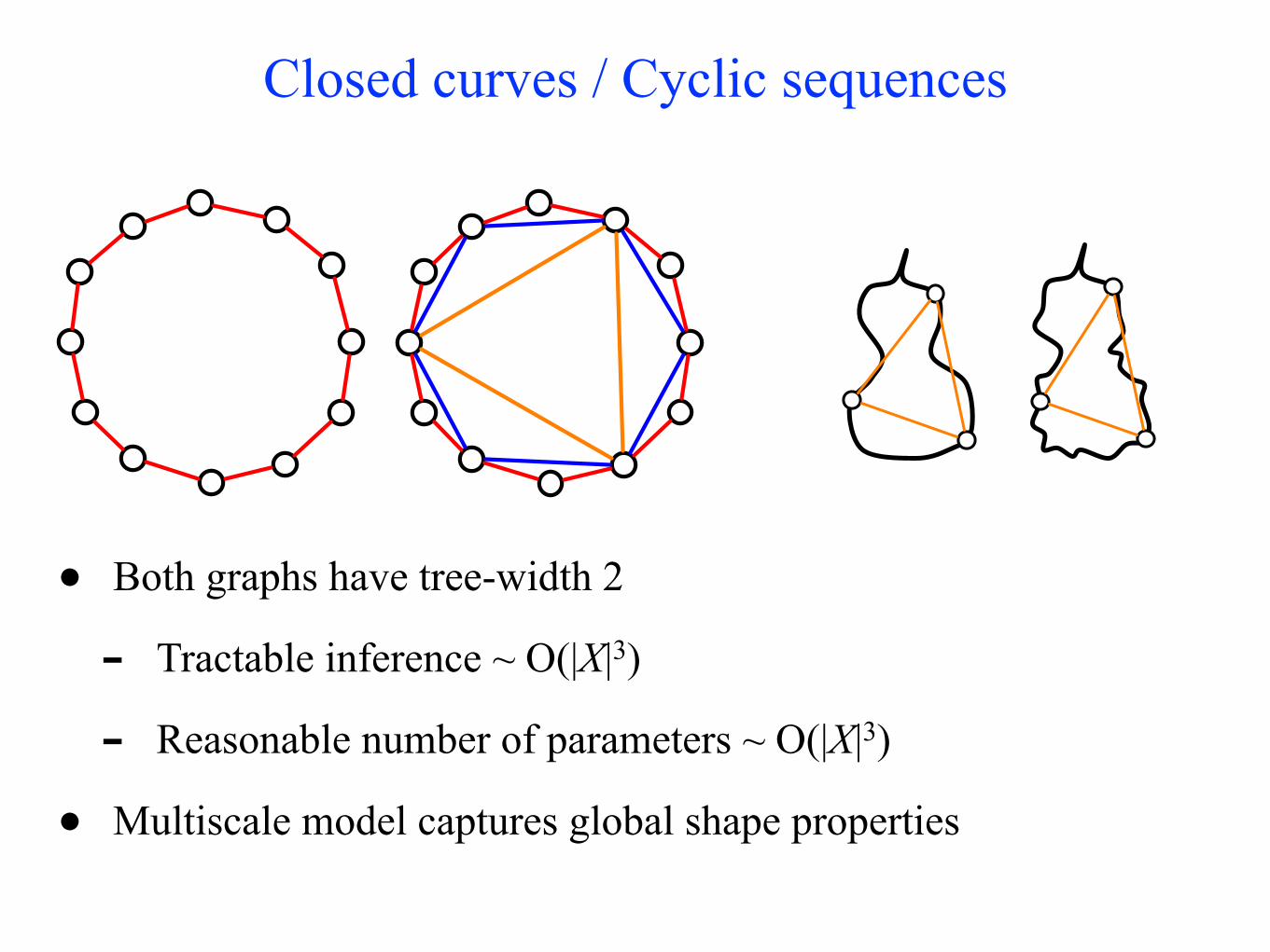
Closed curves / Cyclic sequences

• Both graphs have tree-width 2

- Tractable inference ~ O(|X|3)

- Reasonable number of parameters ~ O(|X|3)

• Multiscale model captures global shape properties

Random deformations

Multiscale model does a good job capturing global shape properties - less drift with similar deformation

Shape recognition

15 species

75 examples per species

(25 training, 50 test)

classification

Multiscale model 96.28

Inner distance 94.13

Shape context 88.12

Swedish leaf dataset

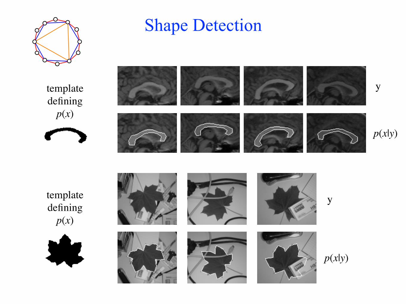
Shape Detection

template defining p(x)

template defining p(x)

y

p(x|y)

y

p(x|y)

Images

• MRF models widely used to model images

• Applications:

• image restoration: clean picture is piecewise smooth

• image segmentation: foreground mask is spatially coherent

p(x) = Ising model

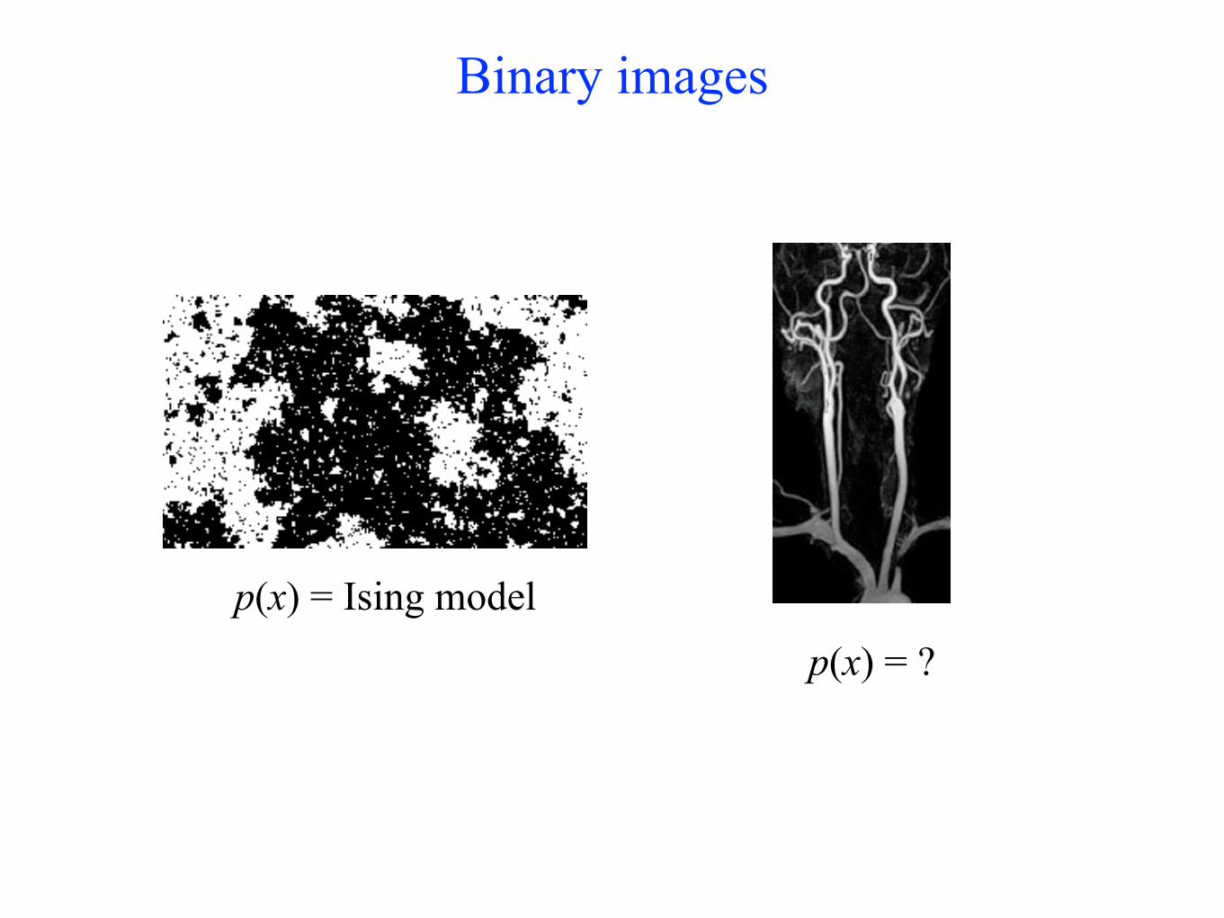
Binary images

p(x) = Ising modelp(x) = ?

Contour maps

• x is a binary image

- pixel is “on” if contour goes through it

• Lots of regularities

- Continuity, smoothness, closure, parallel lines, symmetries

• How can we build a reasonable model for p(x)?

Berkeley Segmentation Dataset

Fields-of-Patterns

• Local property of x ~ binary pattern in 3x3 window

• Look at local properties at multiple resolutions

• Local property of coarse image reflects global properties

(a) (b) (c)

Figure 1: (a) Multiscale/pyramid representation of a contour map. (b) Coarsest image scaled upfor better visualization, with a 3x3 pattern highlighted. The leftmost object in the original imageappears as a 3x3 “circle” pattern in the coarse image. (c) Patches of contour maps (top) that coarsento a particular 3x3 pattern (bottom) after reducing their resolution by a factor of 8.

nary segmentation the prior should encourage spatially coherent masks. In both cases we can designeffective models using maximum-likelihood estimation.

1.1 Related Work

FRAME models [24] and more recently Fields of Experts (FoE) [15] defined high-order energymodels using the response of linear filters. FoP models are closely related. The detection of 3x3patterns at different resolutions corresponds to using non-linear filters of increasing size. In FoP wehave a fixed set of pre-defined non-linear filters that detect common patterns at different resolutions.This avoids filter learning, which leads to a non-convex optimization problem in FoE.

A restricted set of 3x3 binary patterns was considered in [6] to define priors for image restoration.Binary patterns were also used in [17] to model curvature of a binary shape. There has been recentwork on inference algorithms for CRFs defined by binary patterns [19] and it may be possible todevelop efficient inference algorithms for FoP models using those techniques.

The work in [23] defined a variety of multiresolution models for images based on a quad-tree rep-resentation. The quad-tree leads to models that support efficient learning and inference via dynamicprogramming, but such models also suffer from artifacts due to the underlying tree-structure. Thework in [7] defined binary image priors using deep Boltzmann machines. Those models are basedon a hierarchy of hidden variables that is related to our multiscale representation. However in ourcase the multiscale representation is a deterministic function of the image and does not involve extrahidden variables as [7]. The approach we take to define a multiscale model is similar to [9] wherelocal properties of subsampled signals where used to model curves.

One of our motivating applications involves detecting contours in noisy images. This problem has along history in computer vision, going back at least to [16], who used a type of Markov model fordetecting salient contours. Related approaches include the stochastic completion field in [22, 21],spectral methods [11], the curve indicator random field [3], and the more recent work in [1].

2 Fields of Patterns (FoP)

Let G = [n] ⇥ [m] be the grid of pixels in an n by m image. Let x = {x(i, j) | (i, j) 2 G} be ahidden binary image and y = {y(i, j) | (i, j) 2 G} be a set of observations (such as a grayscale orcolor image). Our goal is to estimate x from y.

We define p(x|y) using an energy function that is a sum of two terms,

p(x|y) = 1

Z(y)exp(�E(x, y)) E(x, y) = E

FoP

(x) + Edata

(x, y) (1)

2

x

(a) (b) (c)



1.1 Related Work








p(x|y) = 1


FoP

(x) + Edata

(x, y) (1)

2

Single-scale model

• Energy model

- Look at 3x3 blocks of pixels b

- Each block has one of 512 patterns

- V is an array of 512 costs

• Captures continuity, frequency of 1s, frequency of junctions

• But no smoothness, parallelism, closed curves, etc.

E(x) =X

b

V (xb)

p(x) =1

Z

e

�E(x)

Multi-scale model

• OR pyramid

- x 1 ... x

K

- x i+1 is a coarsening of x

i

• Look at 3x3 blocks at all resolutions

- Vi ≠ Vj

- K arrays of 512 costs

E(x) =X

l

X

b

V

l(xlb)

x1

x2

x3

(a) (b) (c)



1.1 Related Work








p(x|y) = 1


FoP

(x) + Edata

(x, y) (1)

2

(a) (b) (c)



1.1 Related Work








p(x|y) = 1


FoP

(x) + Edata

(x, y) (1)

2

x3

Frequency of Patterns (BSDS)

frequency (high to low) →

reso

lutio

n →

Maximum likelihood model matches frequencies of patterns

Coarse patterns (BSDS)

level 4 24x24

level 5 48x48

Samples from the prior p(x)

(a) (b) (c)

Figure 2: (a) Examples of training images T extracted from the BSD. (b) Samples from a singlescaleFoP prior trained on T . (c) Samples from a multiscale FoP prior trained on T . The multiscale modelis better at capturing the lengths of contours and relationships between them.

image with values in {0, . . . ,M � 1}. The pyramid �(y) is defined in analogy to �(x) except thatwe use a local average for coarsening instead of the logical OR,

yk+1

(i, j) = b(yk(2i, 2j) + yk(2i+ 1, 2j) + yk(2i, 2j + 1) + yk(2i+ 1, 2j + 1))/4c (5)

The data model is parameterized by K vectors D0, . . . , DK�1 2 RM

Edata

(x, y) =

K�1X

k=0

X

(i,j)2Gk

xk

(i, j)Dk

(yk(i, j)) (6)

Here Dk

(yk(i, j)) is an observation cost incurred when xk

(i, j) = 1. There is no need to include anobservation cost when xk

(i, j) = 0 because only energy differences affect the posterior p(x|y).We note that it would be interesting to consider data models that capture complex relationshipsbetween local patterns in �(x) and �(y). For example a local maximum in yk(i, j) might giveevidence for xk

(i, j) = 1, or a particular 3x3 pattern in xk

[i, j].

2.4 Log-Linear Representation

The energy function E(x, y) of a FoP model can be expressed by a dot product between a vector ofmodel parameters w and a feature vector �(x, y). The vector �(x, y) has one block for each scale.In the k-th block we have: (1) 512 (or 102 for invariant models) entries counting the number oftimes each 3x3 pattern occurs in xk; and (2) M entries counting the number of times each possiblevalue for y(i, j) occurs where xk

(i, j) = 1. The vector w specifies the cost for each pattern in eachscale (V k) and the parameters of the data model (Dk). We then have that E(x, y) = w · �(x, y).This log-linear form is useful for learning the model parameters as described in Section 4.

3 Inference with a Band Sampler

In inference we have a set of observations y and want to estimate x. We use MCMC methods [13]to draw samples from p(x|y) and estimate the posterior marginal probabilities p(x(i, j) = 1|y).Sampling is also used for learning model parameters as described in Section 4.

In a block Gibbs sampler we repeatedly update x by picking a block of pixels B and sampling newvalues for x

B

from p(xB

|y, xB

). If the blocks are selected appropriately this defines a Markov chainwith stationary distribution p(x|y).We can implement a block Gibbs sampler for a multiscale FoP model by keeping track of the imagepyramid �(x) as we update x. To sample from p(x

B

|y, xB

) we consider each possible configuration

4

training data single-scale multi-scale

Inference

• Inference with MRF generally hard

• Singlescale FOP

- hard but model is local

• Gibbs sampling

• Loopy BP

• Multiscale FOP

- model not local on x but local on pyramid

Gibbs sampling

• Repeatedly update pixels/blocks

- Sample new value for xq given rest of x

- Requires energy difference between xq = 0 and xq = 1

• Efficient computation using multiscale representation

- Change in xq affects a small number of auxiliary variables

- Energy difference is local over x 1 ... x

K

q

Maximum Likelihood Estimation

• : vector of counts of each pattern at each scale

• : vector of costs

• Training examples x1,..., xn

• Negative log-likelihood is convex

• MLE model:

- expected freq of each pattern = average freq in training data

Ep[�(x)] = �(xi)

�(x)

w

p(x) =1

Z

e

�E(x)E(x) = w · �(x)

Stochastic Gradient Descent

• Estimate expectation by sampling from p

• Mix MCMC simulation with gradient descent

- Let M be Markov chain with stationary distribution p

- Maintain m states s1,..., sm ~ p(x)

• Update model

• Evolve s1,..., sm according to M for a few steps

w

0 = w + ⌘(Ep[�(x)]� �(xi))

w

0 = w + ⌘(�(si)� �(xi))

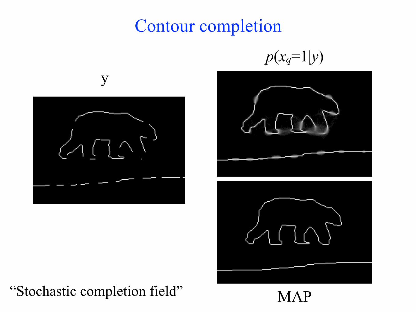
Contour completion

yp(xq=1|y)

MAP“Stochastic completion field”

Contour completion

completion/restoration

iid noise 20% flipped

p(xq=1|y)

y

x

• Standard Markov models capture local properties

• MS models can capture local properties at multiple resolutions

• Local-property of coarse x = global property of x

• Future directions

- coarse-to-fine inference

- non-binary images

- data models

Summary

multiscale models for shapes and images - cs.brown.educs.brown.edu/~pff/talks/multiscale.pdf ·...

Documents