multiscale simulation of heat transfer in a rarefied...

http://wrap.warwick.ac.uk

Original citation: Docherty, Stephanie Y., Borg, Matthew K., Lockerby, Duncan A. and Reese, Jason M.. (2014) Multiscale simulation of heat transfer in a rarefied gas. International Journal of Heat and Fluid Flow . ISSN 0142-727X Permanent WRAP url: http://wrap.warwick.ac.uk/61995 Copyright and reuse: The Warwick Research Archive Portal (WRAP) makes this work of researchers of the University of Warwick available open access under the following conditions. This article is made available under the Creative Commons Attribution 3.0 (CC BY 3.0) license and may be reused according to the conditions of the license. For more details see: http://creativecommons.org/licenses/by/3.0/ A note on versions: The version presented in WRAP is the published version, or, version of record, and may be cited as it appears here. For more information, please contact the WRAP Team at: [email protected]

http://wrap.warwick.ac.uk/

http://wrap.warwick.ac.uk/61995

http://creativecommons.org/licenses/by/3.0/

mailto:[email protected]

International Journal of Heat and Fluid Flow xxx (2014) xxx–xxx

Contents lists available at ScienceDirect

International Journal of Heat and Fluid Flow

journal homepage: www.elsevier .com/ locate/ i jhf f

Multiscale simulation of heat transfer in a rarefied gas

http://dx.doi.org/10.1016/j.ijheatfluidflow.2014.06.0030142-727X/� 2014 The Authors. Published by Elsevier Inc.This is an open access article under the CC BY license (http://creativecommons.org/licenses/by/3.0/).

⇑ Corresponding author. Tel.: +44 7860 366 574.E-mail address: [email protected] (S.Y. Docherty).

Please cite this article in press as: Docherty, S.Y., et al. Multiscale simulation of heat transfer in a rarefied gas. Int. J. Heat Fluid Flow (2014),dx.doi.org/10.1016/j.ijheatfluidflow.2014.06.003

Stephanie Y. Docherty a,⇑, Matthew K. Borg a, Duncan A. Lockerby b, Jason M. Reese c

a Department of Mechanical & Aerospace Engineering, University of Strathclyde, Glasgow G1 1XJ, UKb School of Engineering, University of Warwick, Coventry CV4 7AL, UKc School of Engineering, University of Edinburgh, Edinburgh EH9 3JL, UK

a r t i c l e i n f o a b s t r a c t

Article history:Received 23 December 2013Received in revised form 30 April 2014Accepted 7 June 2014Available online xxxx

Keywords:Heterogeneous multiscale simulationHybrid methodsDSMCHeat flux couplingRarefied gas dynamics

We present a new hybrid method for dilute gas flows that couples a continuum-fluid description to thedirect simulation Monte Carlo (DSMC) technique. Instead of using a domain-decomposition framework,we adopt a heterogeneous approach with micro resolution that can capture non-equilibrium or non-con-tinuum fluid behaviour both close to bounding walls and in the bulk. A continuum-fluid model is appliedacross the entire domain, while DSMC is applied in spatially-distributed micro regions. Using a field-wisecoupling approach, each micro element provides a local correction to a continuum sub-region, the dimen-sions of which are identical to the micro element itself. Interpolating this local correction between themicro elements then produces a correction that can be applied over the entire continuum domain. Keyadvantages of this method include its suitability for flow problems with varying degrees of scale separa-tion, and that the location of the micro elements is not restricted to the nodes of the computational mesh.Also, the size of the micro elements adapts dynamically with the local molecular mean free path. Wedemonstrate the method on heat transfer problems in dilute gas flows, where the coupling is performedthrough the computed heat fluxes. Our test case is micro Fourier flow over a range of rarefaction and tem-perature conditions: this case is simple enough to enable validation against a pure DSMC simulation, andour results show that the hybrid method can deal with both missing boundary and constitutiveinformation.� 2014 The Authors. Published by Elsevier Inc. This is an open access article under the CC BY license (http://

creativecommons.org/licenses/by/3.0/).

1. Introduction

While the conventional hydrodynamic equations are generallyexcellent for modelling the majority of fluid flow problems, thepresence of localised regions of non-continuum or non-equilibriumflow can result in some degree of inaccuracy. Such regions appearwhen the flow is far from local thermodynamic equilibrium, forexample, when there are large gradients in fluid properties, orwhen surface effects become dominant. Although molecular simu-lation tools can provide an accurate modelling alternative in thesecases, they are usually much too computationally expensive forresolving engineering spatial and temporal scales. Multiscalemethodologies that exploit ‘scale separation’ have therefore beendeveloped over the past decade. Scale separation occurs whenthe variation of hydrodynamic properties across small regions ofspace or periods of time is only very loosely coupled with the flowbehaviour on a much larger spatial or temporal scale.

Often referred to as ‘hybrids’, these multiscale methods com-bine continuum and molecular descriptions of the flow. A tradi-

tional continuum description is employed in macro flow regions,and a molecular treatment is applied in small-scale micro or nanoregions. Essentially, the aim is to combine the best of both solvers:the computational efficiency associated with continuum methods,and the detail and accuracy of molecular techniques.

In the literature, two different hybrid frameworks haveemerged for fluid flows: (a) the domain-decomposition technique,and (b) the Heterogeneous Multiscale Method (HMM). For liquids,molecular dynamics (MD) is the appropriate molecular simulationtool. This deterministic method is, however, inefficient for dilutegas flows, and the direct simulation Monte Carlo (DSMC) method(Bird, 1998) can instead provide a coarse-grained moleculardescription. Founded on the kinetic theory of dilute gases, DSMCreduces computational expense by adopting a stochastic approxi-mation for the molecular collision process.

Typically, thermodynamic non-equilibrium effects occur in thevicinity of bounding surfaces or other interfaces. Recognising thisbehaviour, domain-decomposition has become the most popularhybrid framework for both liquids (O’Connell and Thompson,1995; Hadjiconstantinou and Patera, 1997; Flekkøy et al., 2000;Delgado-Buscalioni and Coveney, 2003; Werder et al., 2005) anddilute gases (Wadsworth and Erwin, 1990; Hash and Hassan,

http://



http://dx.doi.org/10.1016/j.ijheatfluidflow.2014.06.003


mailto:[email protected]


http://www.sciencedirect.com/science/journal/0142727X

http://www.elsevier.com/locate/ijhff



2 S.Y. Docherty et al. / International Journal of Heat and Fluid Flow xxx (2014) xxx–xxx

1996; Garcia et al., 1999; Aktas and Aluru, 2002; Roveda et al.,1998; Sun et al., 2004; Sun and Boyd, 2002; Wijesinghe et al.,2004; Wu et al., 2006; Schwartzentruber et al., 2007; Lian et al.,2008). In this method, the simulation domain is partitioned — amolecular solver is applied in the regions closest to the surfaces,while a conventional continuum fluid solver is implemented inthe remainder. These micro and macro sub-domains are indepen-dent but communicate through an overlap region that enablesmutual coupling. This coupling is typically established by matchingfluxes of fluid mass, momentum, and energy, or by matching stateproperties. However, despite its popularity, a fundamental disad-vantage of this micro–macro decomposition approach is that com-putational efficiency can only be increased above that of a fullmolecular simulation when non-continuum flow is confined to‘near-wall’ regions. In highly non-equilibrium flows, or when thetemperature dependence of fluid properties such as dynamic vis-cosity or thermal conductivity is not known a priori (for example,in unusual chemically-reacting gas mixtures), the traditional fluidconstitutive relations may be inaccurate in the bulk of the domain.

Domain-decomposition techniques are also inappropriate forsimulating flow through micro or nanoscale geometries that havea high aspect ratio, e.g. one dimension of the geometry is ordersof magnitude larger than another. This class of flow presents achallenge as it requires simultaneous solution of the microscopicprocesses occurring over the smallest dimension and the macro-scopic processes occurring over the largest dimension, and is oftentoo computationally intensive for a full molecular approach. Suchflows are generally beyond the reach of domain-decompositionas the majority (or perhaps all) of the flowfield can be considered‘near-wall’.

The less-common HMM framework overcomes the limitationsof domain-decomposition by adopting a micro-resolutionapproach that can be employed anywhere in the domain — nearbounding surfaces, or in the bulk flow. In this case, a continuummodel is applied across the entire flow field, and the molecular sol-ver is applied in spatially-distributed micro regions. These microregions provide the missing data that is required for closure ofthe local continuum model, either in the form of unknown bound-ary conditions, or unknown constitutive information. ExistingHMM studies in the literature are mainly for liquid flows, usingMD as the molecular solver (Ren and E, 2005; Yasuda andYamamoto, 2008; Asproulis et al., 2012; Borg et al., 2013). Gener-ally, these studies consider flow problems where momentumtransport is dominant and the transfer of heat is negligible. Cou-pling is therefore based on momentum: velocity fields or strain-rates are prescribed in each micro region, and the resultant stressis used to apply a correction back into the hydrodynamic momen-tum equation (Ren and E, 2005; Yasuda and Yamamoto, 2008).Each HMM micro region supplies information to a computationalnode on the continuum mesh. This point-wise coupling approach(Asproulis et al., 2012) is ideal when there is a large degree of spa-tial scale separation in the system, providing significant computa-tional savings over a pure molecular simulation. However, in flowproblems with smaller, or mixed, degrees of spatial scale separa-tion, the molecular resolution required can result in the micro ele-ments overlapping, making HMM more expensive and lessaccurate than a pure molecular treatment.

Despite its advantages over domain-decomposition techniques,there has been little development of HMM-type hybrids that useDSMC as the molecular treatment. In 2010, Kessler et al. (2010)proposed the Coupled Multiscale Multiphysics Method (CM3) thatcouples both momentum and heat transfer, with DSMC providingcorrections to both the hydrodynamic momentum and energyequations. This method was, however, developed to simulate tran-sient flows where a time-accurate solution is sought, and so anycomputational advantage over a full DSMC simulation is achieved

Please cite this article in press as: Docherty, S.Y., et al. Multiscale simulationdx.doi.org/10.1016/j.ijheatfluidflow.2014.06.003

only through decoupling of the time scales; the length scalesremain fully coupled, with both the continuum description andDSMC employed over the same region of space. More recently,Patronis et al. (2013) adapted the Internal-flow Multiscale Method(IMM) to simulate dilute gas flows with DSMC. Originally devel-oped by Borg et al. (2013) for liquid flows, IMM adopts a frame-work similar to HMM but is tailored to model flows in high-aspect-ratio channels. Although large computational savings arepresented, this method is tailored specifically to deal with caseswhere the length scale in the direction of flow is significantly largerthan the length scales transverse to the flow direction.

In this paper we propose a new form of the HMM technique,with DSMC providing the molecular description. We adopt the fieldwise coupling (HMM–FWC) approach developed by Borg et al.(2013) for liquid flows: rather than supplying a correction to anode on the continuum mesh, each micro element instead correctsa continuum sub-region, the spatial dimensions of which are iden-tical to those of the micro element itself. This means that, unlikepoint wise coupling, HMM–FWC is suitable for dealing with flowproblems with varying degrees of spatial scale separation. Also,the location of each micro element is not restricted to the nodesof the computational mesh: both the position and size of the microelements can be optimised for each problem, independently of thecontinuum mesh.

Our method is designed to cope with inaccuracy in the tradi-tional flow boundary conditions and/or constitutive relations,and is therefore able to deal with problems that are beyond thereach of domain-decomposition. This includes problems wherethe fluid behaviour is unknown in the bulk, i.e. the traditional con-stitutive relations fail due to non-equilibrium effects (for example,in the wake of a re-entry vehicle), or the transport properties areunknown (for example, in unusual gas mixtures). The method isalso suitable for simulating high aspect ratio geometries. Whilethe IMM is designed to simulate problems where the largest lengthscale is in the flow direction, our new method has no such restric-tion and so provides a more general approach. It could therefore beuseful when the largest length scale is transverse to the flow direc-tion; for example, the flow through microscale cracks that canappear in valves.

The form of the method we present in this paper is tailored tomodel heat transfer problems in dilute gas flows. As a startingpoint we consider problems in which the gas is essentially motion-less, with large applied temperature gradients placing the focus onheat transfer. With negligible transport of momentum, our cou-pling is performed through the heat flux: we impose the local tem-perature fields on the micro elements and measure the consequentheat flux from the relaxed DSMC particle ensembles. A suitablecorrection is then applied to the hydrodynamic conservation ofenergy equation. (Full coupling of mass, momentum, and heattransfer is a subject for future work.)

The level of translational non-equilibrium in a rarefied gas isgenerally characterized by the Knudsen number Kn, defined asthe ratio of the gas molecular mean free path k to a characteristicsystem dimension L. Typically, the traditional ‘no-temperature-jump’ boundary condition at a bounding surface (wall) is only validwhen Kn < 0:001; the flow is then in thermodynamic equilibriumas the frequency of both intermolecular and molecule-wall colli-sions is very high. As Kn increases above 0:001, this collision fre-quency decreases, resulting in a temperature discontinuitybetween the wall and its adjacent gas. For low Kn, the conventionalconservation equations can be extended to account for this byemploying von Smoluchowski temperature-jump boundary condi-tions (von Smoluchowski, 1898). However, as Kn increases, mole-cule-wall collisions become more frequent than intermolecularcollisions and the thermal Knudsen layer becomes significant. Thisis essentially a region of non-equilibrium that extends from the

of heat transfer in a rarefied gas. Int. J. Heat Fluid Flow (2014), http://



S.Y. Docherty et al. / International Journal of Heat and Fluid Flow xxx (2014) xxx–xxx 3

wall into the domain, with its thickness determined by the degreeof rarefaction. In this layer, the gas behaviour deviates from theconventional linear heat-flux/temperature-gradient constitutiverelation. Even with the use of temperature-jump boundary condi-tions, the conventional hydrodynamic equations cannot model thisphenomenon. Our hybrid method, however, aims to capture boththe temperature-jump and the thermal Knudsen layer at a lowercomputational cost than a full-domain DSMC treatment.

This paper is organised as follows. In Section 2, we discuss themacro and micro descriptions of the flow. We then present thegeneral three-dimensional form of our multiscale coupling frame-work and its iterative algorithm. For simplicity, one-dimensionalheat transfer is considered when validating the method in Sec-tion 3, with results compared with pure DSMC simulations atequivalent conditions. In Section 4 we draw our conclusions.

2. Multiscale methodology

2.1. Continuum description

For simplicity in this paper we restrict our attention to steady-state problems where the gas remains stationary, i.e. it has nostreaming velocity. With negligible transport of mass and momen-tum, the continuum description is based on the conservation ofenergy,

r � q ¼ 0; ð1Þ

where q is the heat flux vector. To close this equation, a suitableconstitutive relation is required. For conventional gas flows, the tra-ditional Navier–Stokes-Fourier (NSF) constitutive relations areaccurate and so Fourier’s law can be used, i.e.

q ¼ �jrT; ð2Þ

where j is the thermal conductivity of the gas. The energy equationthen reads,

r � ðjrTÞ ¼ 0: ð3Þ

Assuming no-temperature-jump boundary conditions, solution ofthis conventional energy equation will produce a continuum NSFtemperature field TNSF. This field is taken as an initial conditionfor our hybrid method, and provides a starting point from whichthe coupling framework iterates towards the correct temperaturefield.

While Eq. (2) is valid for typical flow problems, it fails in certainflow conditions, for instance, in flows of complex fluids or in con-ditions of thermodynamic non-equilibrium. Inaccuracy in the con-ventional constitutive model can therefore be quantified by a heat-flux-correction field U, so that

q ¼ �jrT þU: ð4Þ

The flux-correction field incorporates not only the departure of thegas state from equilibrium, but also any additional inaccuracy dueto the assumed thermal conductivity model. Using this relation toclose Eq. (1) results in a ‘flux-corrected’ energy equation,

r � ðjrTÞ � r �U ¼ 0: ð5Þ

The general strategy of our heterogeneous hybrid approach is there-fore as follows. Across each individual micro element, the heat fluxand temperature fields are measured. The flux-correction fieldacross each element is then computed using Eq. (4). By interpolat-ing between all micro elements, the full flux-correction field Uacross the entire flowfield is approximated. With this, and theboundary information obtained from micro simulations located atthe bounding walls, an appropriate continuum method (e.g. finitedifference, finite element, or finite volume) can be used to solveEq. (5). This produces a flux-corrected continuum temperature field


TU across the domain. With continuing iterations, this temperaturefield should converge towards that which would be obtained from afull molecular simulation of the problem.

2.2. DSMC technique

As we focus on heat transfer in dilute gases, we use DSMC as ourmolecular model in the micro elements. DSMC has become thedominant method for simulating dilute gas flows that lie in thecontinuum-transition regime. The fundamental concept is to tracka large number of numerical particles, storing their position, veloc-ity, and internal state as they move through a computational mesh.During a simulation, the particles collide with each other and withbounding surfaces while maintaining conservation of mass,momentum, and energy. A major advantage of the method is thattwo key approximations significantly reduce computationalexpense: (a) each simulated particle typically represents a largenumber of real gas molecules, and (b) molecular motion and inter-molecular collisions can be decoupled over small time intervals.Particle movements are computed deterministically, while inter-particle collisions are treated statistically within numerical meshcells.

Using expressions provided by Bird (1998), local hydrodynamicproperties (including the temperature and the heat flux) can berecovered in DSMC by averaging microscopic data over all of theparticles in each cell. However, the inherent statistical scatter asso-ciated with the method means that a large number of independentsamples are usually required to capture smooth fields, particularlyfor low speed flows. Therefore, time averaging is typically used forsteady state problems, while ensemble averaging is used for tran-sient flow problems. For continuum-molecular hybrids, thesmoothing of statistical fluctuations is particularly important asthe transfer of noisy data to the continuum fluid description mayresult in instability. Consequently, each DSMC simulation in thispaper is performed in two stages: a transient period enables thesimulation to reach steady-state, and then a longer averaging per-iod reduces the statistical scatter in the measured hydrodynamicproperties.

The open-source C++ toolbox OpenFOAM (2013) incorporates aDSMC solver, dsmcFoam, which has been validated for variousbenchmark cases, including hypersonic and microchannel flows(Scanlon et al., 2010; Arlemark et al., 2012; White et al., 2013). Thisis used to perform all of the micro and full-scale DSMC simulationsin this paper.

2.3. Coupling framework

In our framework, the continuum description is applied acrossthe entire macro domain, while DSMC is performed in dispersedmicro elements (the arrangement of which depends on the flowproblem being investigated). As discussed in the Introduction, wepropose a new strategy to achieve two-way coupling betweenthese domains. The underlying methodology presented here isgeneral and may be applied to 1D, 2D, or 3D problems.

2.3.1. Macro-to-micro coupling: constraint of the micro elementsIt is crucial that the flux-correction information is extracted

from DSMC elements in which the gas state is properly representa-tive of the local conditions in the macro domain. There is, however,a fundamental problem in creating such elements: the particle dis-tribution required at the boundaries of the element cannot beextracted directly from the macroscopic continuum flowfield. Forthis reason, macro-to-micro coupling remains a challenge in mul-tiscale hybrids. In our method, we circumvent this problem bynot imposing an exact particle distribution at these boundaries;




Relaxation zone

Sampling zone

Imposed particle distribution

Solid wall

near-wall micro element


bulk micro element

continuum mesh

control cells

measurement cells

(a)

(b)

Fig. 1. Schematic of (a) a 2D bulk micro element showing the control and measurement cells, and (b) an example computational domain for a 2D problem. The control andmeasurement cells are independent of the DSMC computational cells, and can also be independent of the continuum mesh.


instead, we allow the distribution to be dictated by the macro-scopic continuum fields alone.

A natural evolution to the correct particle distribution and mac-roscopic state at the boundaries of an element is possible by estab-lishing an artificial relaxation region (zone) around the element. Itis not essential that the gas state in these relaxation zones accu-rately represent the conditions in the corresponding macrodomain; their sole purpose is to develop the boundary conditionsfor the core of the element. Sampling of property fields is per-formed only in the core region, which we refer to as the ‘samplingzone’.

Suitable boundary conditions to the sampling zone are gener-ated by enforcing the continuum variation of macroscopic proper-ties (i.e. in our case, the continuum temperature field) across thesurrounding relaxation zone. This is done by implementing particlecontrollers (Borg et al., 2010). A particle distribution does, how-ever, need to be applied at the outer boundaries of the relaxationzone. This imposed distribution introduces error in the local distri-bution close to these boundaries, and so it is important that theparticle state within the sampling zone is sufficiently independentof this introduced error. If the relaxation zone is large enough (i.e.several molecular mean free paths), the form of the imposed distri-bution1 is irrelevant — its effect will decay through the zone as theparticle state gradually relaxes through interparticle collisions. Com-

1 We implement local Maxwellian distributions at the outer edges of the relaxationzones for simplicity. Chapman–Enskog distributions could also be used; as theseinclude perturbations from equilibrium, they may reduce the required size of therelaxation zones.


plete relaxation needs to occur over the extent of the relaxation zonesuch that the particle distribution in the sampling zone is dictatedsolely by the applied continuum state. Once the hybrid methodhas converged, the artificiality of the outer relaxation zone dissolvesseamlessly into the true particle distribution and fluid state in theinner sampling zone.

Fig. 1a shows a typical ‘bulk’ micro element in 2D. Similarly,Fig. 1b shows an example computational domain set-up for a 2Dproblem, including both bulk and ‘near-wall’ micro elements. Insummary, the sampling zone in a micro DSMC element is sur-rounded by the relaxation zone over which the local continuumfields are imposed, and a chosen particle distribution is appliedat the outer boundaries. However, in order to capture regions ofnon-equilibrium that often appear at solid bounding surfaces orwalls, the sampling zone in a near-wall micro element must beadjacent to the wall itself. The arrangement of the micro elementsis clearly crucial to the overall accuracy of our method, and theappropriate arrangement will vary from problem to problem.

To impose the local continuum temperature field, we divide therelaxation zone in each micro element into a grid of control cells asshown in Fig. 1. Using particle controllers (Borg et al., 2010), theappropriate temperature is then set in each control cell to createthe desired temperature variation. Similarly, the sampling zoneof each micro element is divided into a grid of measurement cells.We then extract the averaged hydrodynamic properties from eachmeasurement cell, enabling us to capture the property fields acrossthe entire sampling zone. Boundary information is also obtainedfrom these measurement cells: we extract the temperature of thegas in contact with the wall from the wall-adjacent cell faces.





Essentially, these measurement and control cells form a mea-surement/control mesh that is completely independent of the com-putational mesh used by DSMC itself. This has the benefit ofenabling us to define the resolution of the macroscopic fields thatwe both extract and impose, and to control the noise in our mea-surements, without affecting the accuracy of the DSMC calcula-tions (i.e. the particle collision rate). In Fig. 1, the measurementand control cells are shown to have the same dimensions, but thisdoes not have to be the case. Also, in Fig. 1b, the measurement andcontrol cells are shown to be collocated with the computationalcells of the continuum mesh; although this simplifies the transferof data between the micro elements and the continuum descrip-tion, it is only for convenience and is not essential. If these cellsare not collocated, we simply interpolate between the meshes.

2.3.2. Micro-to-macro coupling: correcting the continuum descriptionThe ease in converting microscopic particle information into

macroscopic fields means that, generally, micro-to-macro couplingis less problematic than macro-to-micro coupling. Based on theproperty fields extracted from the DSMC solver, a suitable correc-tion can be applied to the continuum description. In our couplingstrategy, this correction is in the form of a heat-flux-correctionfield U, as discussed in Section 2.1.

In our DSMC simulations, the average translational temperature(for a single species gas) in each measurement cell is computed from,

Ttr ¼1

3kBmc02 ¼ 1

3kBm c02x þ c02y þ c02z� �

; ð6Þ

where kB is the Boltzmann constant, m is the molecular mass andc0x; c0y, and c0z are the x; y, and z components of the thermal velocityvector c0. Assuming the gas has no vibrational energy, the averageheat flux q in each measurement cell is obtained from,

q � qj ¼12

mnc02c0j þ nerotc0j; ð7Þ

where j represents the x; y, and z components, n is the number den-sity of the gas, and erot is the rotational energy of a single molecule.Note that we consider monatomic gas flows in this paper, and soerot ¼ 0 and the macroscopic temperature T ¼ Ttr . By computingthe average macroscopic temperature and heat flux in each mea-surement cell, we capture the temperature and heat flux fieldsacross the sampling zone of each micro element. Substituted intoEq. (4), these then provide the flux-correction field across this zone.However, the continuum description is applied across the full sim-ulation domain, and so Eq. (5) requires the flux-correction fieldacross the full domain. This field can be approximated using appro-priate interpolation between all the sampling zones.

This hybrid methodology not only corrects for inaccurate con-stitutive information, but also provides missing boundary informa-tion, i.e. the temperature jump. In each near-wall sampling zone,we measure the temperature of the gas in contact with the wallby summing over all particles that strike the surface (Lofthouse,2008), i.e.

Tgas;wall ¼m

3kB

P½ðm=jcnjÞðkckÞ� �

Pðm=jcnjÞU2

slipPð1=jcnjÞ

; ð8Þ

where cn is the particle velocity normal to the wall, ct is the particlevelocity tangential to the wall, kck is the velocity magnitude, andUslip is the slip velocity which, with zero wall velocity, is given by

Uslip ¼P½ðm=jcnjÞct �Pðm=jcnjÞ

: ð9Þ

We then interpolate this boundary gas temperature between thenear-wall sampling zones to produce an estimate of the gas temper-ature at all bounding surfaces.


Using this boundary information and the full flux-correctionfield U, solution of Eq. (5) then produces a new (flux-corrected)temperature field TU across the whole domain. The process is thenrepeated until TU relaxes to a solution that is close to that obtainedfrom a full DSMC simulation.

2.4. Iterative algorithm

The general iterative coupling procedure of this method is:

(0) Assuming no-temperature-jump at bounding surfaces, solvethe conventional energy equation (3) to obtain an initialestimate for the temperature field across the entire simula-tion domain, TNSF.

(1) Constrain each micro element by applying boundaryconditions:
(a) Using particle control in each control cell, enforce thelocal continuum temperature variation throughout therelaxation zone.(b) At the outer boundaries of the relaxation zone, imposeMaxwellian particle distributions at the local continuumtemperature.
(2) Execute DSMC in each micro element as described in Sec-tion 2.2. When steady-state is reached, perform averagingof properties in all measurement cells across the samplingzone of each element. Extract the temperature and the heatflux values from each of these cells. Also, from each wall-adjacent measurement cell face, extract the temperature ofthe gas at the wall surface.

(3) Compute the flux-correction in each measurement cell usingthe temperature and heat flux values extracted from thatcell in the flux-corrected constitutive relation (4). From this,obtain the flux-correction field across each sampling zone.

(4) Carry out appropriate interpolations between samplingzones to approximate the flux-correction field U across thefull simulation domain. Similarly, perform appropriate inter-polations between near-wall sampling zones to obtain thegas temperature at all bounding walls.

(5) Using the boundary gas temperature information and thefull flux-correction field, solve the flux-corrected energyequation (5) across the full domain to obtain a new flux-cor-rected temperature field TU.

(6) Repeat from Step (1) until TU does not change between iter-ations to within a user-defined tolerance.

3. Validation: one-dimensional Fourier flow

A simple test case is chosen in order to assess the performanceof the coupling method, and to easily validate it against a fullDSMC simulation. We demonstrate the method on the case ofone-dimensional heat transfer, i.e. the classical Fourier flow prob-lem. This problem has a motionless gas (in this case argon) con-fined between two infinite parallel planar walls with differenttemperatures, Tcold and Thot.

3.1. Numerical implementation

We assume that the variation of the gas thermal conductivity jwith temperature is unknown. We therefore take a reasonable ref-erence value jr that is independent of the temperature field acrossthe system domain; as discussed in Section 2.1, the flux-correctionfield U will automatically adjust for any error resulting from thisassumption.

Discretizing the domain in one-dimensional space, the macro-scopic computational mesh consists of N macro nodes, includinga node at each wall. An example computational domain set-up is




Sampling zone

Relaxation zoneImposed particle distributionSolid wall

∆x

bulk micro element



∆xL

x

Tcold Thot

Fig. 2. Schematic of the computational set-up for a one-dimensional Fourier flow problem.


shown in Fig. 2, where we have a micro element at each wall, andone in the bulk. This element arrangement is an example only —the appropriate arrangement will in practise depend on the caseitself, as will be discussed further in Section 3.2.1. For this 1D prob-lem, each near-wall element comprises a single sampling zone anda single relaxation zone, while each bulk element consists of a sin-gle sampling zone with a relaxation zone on either side, as indi-cated in Fig. 2.

Each sampling zone is divided into a number of measurementbins. Similarly, each relaxation zone is divided into a number ofcontrol bins. To keep the transfer of data between the macroscopicmesh and the micro elements as simple as possible, the binarrangement in each element is set such that the centre of eachbin coincides exactly with a macro node, i ¼ 1;2; . . . ;N. Again thisis merely for convenience, and does not generally need to beimposed. The length of each 1D bin is then equal to the spacingbetween each macro node, Dx.

Application of the general coupling algorithm of Section 2.4 tothis 1D system is as follows:

(0) An initial estimate for the temperature field across the sim-ulation domain is computed by solving the 1D conservationof energy equation,

Pleasedx.doi

dqx

dx¼ 0; ð10Þ

where qx is the streamwise component of the heat flux vec-tor. This expression can be closed using the 1D form of Fou-rier’s law,

qx ¼ �jdTdx

� �: ð11Þ

With the reference thermal conductivity jr , the 1D energyequation becomes,

jrd2T

dx2

" #¼ 0; ð12Þ

and can be approximated using a second-order central finitedifference scheme. With no temperature-jump at the solidwalls (i.e. T1 ¼ Tcold and TN ¼ Thot), solution results in the ini-tial continuum temperature field TNSF.

(1) As the micro element size can change at each iteration (aswill be discussed in Section 3.2.1), each element is initialisedat equilibrium before boundary conditions are applied. Thisis done by sampling particle velocities from a Maxwelliandistribution. For consistency between the micro and macrodomains, the temperature and density for initialisation areobtained from the local continuum solution: continuum val-ues of these properties are averaged over a sub-region of themacro domain that corresponds to the particular micro ele-ment.Each micro element is then constrained:

cite this article in press as: Docherty, S.Y., et al. Multiscale simulation.org/10.1016/j.ijheatfluidflow.2014.06.003

(a) The local continuum temperature field is imposedthroughout each relaxation zone by implementing a thermo-stat in each control bin.(b) Maxwellian particle distributions are imposed at theouter boundaries of each relaxation zone via a diffuse solidwall condition at the local continuum temperature.

(2) DSMC is executed in each micro element. When steady-stateconditions are reached, time averaging of properties is per-formed in each measurement bin. From each bin, time-aver-aged values of the temperature and the heat flux areextracted. Also, from both near-wall sampling zones, thetemperature of the gas in contact with the bounding wallis extracted.

(3) Using the temperature and the heat flux extracted from eachmeasurement bin, the flux-correction in each bin can becomputed by applying the 1D flux-corrected constitutiverelation with constant conductivity jr ,

Ux ¼ qx þ jrdTdx

� �: ð13Þ

For this calculation, the temperature gradient in each mea-surement bin is approximated using a central finite differ-ence scheme (or a forward/backward finite differencescheme for bins at the edges of the sampling zone). By com-puting the flux-correction in each measurement bin, theflux-correction field across each sampling zone is captured.

(4) To obtain Ux at every point in the domain, interpolationbetween sampling zones is required. A study was performedshowing that a simple linear interpolation provides an ade-quate representation of the full flux-correction field for this1D case. Note that, for this 1D geometry, interpolation of theboundary gas temperature is not required.

(5) Using Eq. (13) to close Eq. (10) provides the 1D flux-cor-rected energy equation,

jrd2T

dx2

" #� dUx

dx¼ 0; ð14Þ

which can be approximated using a second-order centralfinite difference scheme. As discussed in Section 2.3.2, tem-perature-jump boundary conditions are applied: the tem-perature of the gas at each bounding wall is set to be thatmeasured in the corresponding near-wall element duringStep (2). Solving this equation then results in the flux-cor-rected temperature field TU across the entire domain.

(6) Replacing the initial temperature field TNSF with TU, the pro-cess is repeated from Step (1). This continues until TU con-verges to within a user defined tolerance, i.e.

of

f ¼ 1N

XN

i¼1

TUðiÞl � TUðiÞl�1

TUðiÞl

�� 6 ftol; ð15Þ

where N is the number of macro nodes, l is the iterationindex, and ftol is the tolerance parameter.

heat transfer in a rarefied gas. Int. J. Heat Fluid Flow (2014), http://




3.2. Results

The overall level of non-equilibrium in the gas is characterizedhere by a global Knudsen number Kn, where the characteristicdimension is the separation between the heated walls L, i.e.

Kn ¼ kL: ð16Þ

We use a Variable Hard Sphere (VHS) collision model in our DSMCsimulations, and so the gas mean free path is given by (Bird, 1998),

k ¼ 1ffiffiffi2p

pd2n; ð17Þ

where d is the VHS molecular diameter, and n is the number densityof the gas. Localised regions of non-equilibrium can also result fromlarge gradients in the macroscopic fluid properties, for example,temperature gradients. Varying both Kn and the temperature gradi-ent across the system, we simulate a range of test cases here. Theseexplore the ability of the hybrid method to deal with both missingconstitutive and boundary information, while remaining simpleenough for validation against an equivalent full-scale DSMCsimulation.

For simplicity, we simulate monatomic argon gas with the fol-lowing VHS parameters: a reference temperature Tref ¼ 273 K, areference diameter dref ¼ 4:17� 10�10 m, and viscosity exponentx ¼ 0:81. For all test cases, the separation between the walls L is1 lm. In order to accurately capture the variation of the propertyfields, we set the number of macro nodes N across the domain tobe 201 for all cases, making the constant spacing Dx between eachmacro node 5 nm. For each test case, we then set the gas densityand the temperature of the walls to obtain the desired Kn and tem-perature gradient.

To ensure a fair comparison between each hybrid simulationand the equivalent full-scale DSMC simulation, we use the samecell-size and time-step in both the hybrid DSMC elements andthe full-scale simulation. The cell size is set as a fraction of thegas mean free path k. The DSMC time-step must be a fraction ofthe mean collision time tmc: a time-step Dt ¼ 1� 10�12 s is suffi-ciently small for all cases simulated in this paper. In our testing,we found that an initial start-up run of 3 million time-stepsallowed all DSMC simulations to reach steady state. To minimisethe statistical scatter associated with the averaging of the fieldproperties, all simulations were then run for a further 50 milliontime-steps.

As discussed in Section 3.1, we monitor convergence of thehybrid procedure using Eq. (15), which quantifies the differencein the temperature solution between the current iteration andthe previous. The tolerance parameter ftol depends on the caseitself, with typical values of Oð10�2Þ and below. We then requirea measure of the overall accuracy for the converged hybrid solutionwhen comparing with the corresponding full-scale DSMC solutionTFull. Here we consider the mean percentage error �� in the hybridtemperature profile, i.e.

�� ¼ 1N

XN

i¼1

TFullðiÞ � TUðiÞTFullðiÞ

� �� 100%: ð18Þ

The value of this error depends on the hybrid’s ability to capture the‘true’ flux-correction field across the simulation domain. The trueflux-correction is that which can be computed from the full-scaleDSMC solution Ux;Full, using the measured temperature field TFull

and the measured heat flux field qx;Full in Eq. (13).

3.2.1. Micro resolutionThe temperature-jump and associated thermal Knudsen layer

are modelled within the micro element at each wall. To obtain a


high level of accuracy for this Fourier flow problem, the samplingzone in each of these elements should extend to capture the entireKnudsen layer. This means that the required size of our near-wallelements increases with the level of rarefaction, i.e. Kn. Note that,for high values of Kn, the required size of the near-wall micro ele-ments may result in the hybrid approach (over a number of itera-tions) becoming less efficient than a full-scale DSMC treatment. Forlow values of Kn (where the Knudsen layers remain close to thewalls), micro elements could be required in the bulk to capturenon-equilibrium behaviour caused by strong temperature gradi-ents. Even when the bulk of the domain is near-equilibrium, bulkmicro elements may still be needed to provide a correction forany error in the assumed thermal conductivity jr . The micro reso-lution (i.e. the number of micro elements P and their size)required for a particular problem is therefore dependent on boththe level of rarefaction, and the temperature conditions.

To explore the effect of the micro element arrangement, weconsider an example test case with Kn = 0.01. For a separationL = 1 lm, we require a global mean free path k ¼ 0:01 lm, corre-sponding to a gas number density n = 1.295 � 1026 m�3 from Eq.(17). Setting an average gas temperature Tav ¼ 273 K, we assumea value of jr ¼ 0:0164 W=m K (Younglove and Hanley, 1986). Thetemperature difference between the walls DT is set to 50 K (i.e.Tcold ¼ 248 K and Thot ¼ 298 K), resulting in a temperature gradientof 50 � 106 K/m across the domain.

For this initial test case, with this Knudsen number and temper-ature gradient, the bulk of the domain will be in equilibrium. How-ever, the flux-correction field Ux in the bulk will be non-zero tocorrect for the assumption of a constant thermal conductivity. Overa temperature range of 200 K to 350 K, the thermal conductivity ofargon varies approximately linearly with temperature, so Ux willalso be approximately linear in the bulk. Direct linear interpolationbetween the sampling zones of the near-wall elements shouldtherefore provide an adequate representation of the full flux-cor-rection field, and bulk micro elements are not needed for this ini-tial case. Two near-wall elements should be sufficient, i.e. P ¼ 2.

Ideally, the sampling zones of these near-wall micro elementsshould capture the thermal Knudsen layers fully. Also, the relaxa-tion zones must be large enough to allow complete relaxation ofthe particle distribution. The size of both of these zones is thereforekey to the accuracy of the hybrid method, and it is important thatwe are able to make an estimate of the appropriate size dependingon the flow conditions. Typically, thermal Knudsen layers extendseveral mean free paths from a wall surface. Similarly, particlerelaxation typically occurs over several mean free paths. We there-fore express the extents of both the sampling and relaxation zonesin terms of the local mean free path kl.

Two sensitivity studies have been performed to find the appro-priate extent for each zone. In the first study, we keep the length ofthe sampling zone LSZ at 5kl and consider the effect of the relaxa-tion zone length LRZ by incrementally increasing its value from1kl to 7kl. Then, in the second study, we consider the impact ofLSZ by increasing it from 1kl to 7kl, keeping LRZ constant at 5kl. Notethat, for the first iteration, kl is assumed equal to the global meanfree path, k ¼ Kn L. In subsequent iterations, kl is updated for eachmicro element using Eq. (17), where n is the average number den-sity measured in the sampling zone of the element in the previousiteration.

With elements in this size range, we need to see convergence ofthe hybrid method within 3 to 4 iterations for there to be any com-putational advantage over a full DSMC simulation. For this testcase, we set the tolerance parameter ftol to be 0.001. Fig. 3a showsthat, for all relaxation zone lengths, convergence of the method isreached within 4 iterations. However, convergence is not reachedwithin 4 iterations when the sampling zone lengths are 1kl or3kl, as shown in Fig. 3b. We therefore require larger sampling zones




0

0.001

0.002

0.003

0.004

1 2 3 4

(a) LRZ = 1λl

LRZ = 3λl

LRZ = 5λl

LRZ = 7λl

0

0.001

0.002

0.003

0.004

1 2 3 4

(b) LSZ = 1λl

LSZ = 3λl

LSZ = 5λl

LSZ = 7λl

Fig. 3. Convergence of the hybrid method for (a) LSZ ¼ 5kl and various LRZ , and (b)LRZ ¼ 5kl and various LSZ .

255

270

285

300

0 0.2 0.4 0.6 0.8 1

(a)

TFull

TNSF

TΦ (LRZ = 1λl)

TΦ (LRZ = 3λl)

TΦ (LRZ = 5λl)

TΦ (LRZ = 7λl)

255

270

285

300

0 0.2 0.4 0.6 0.8 1

(b)

TFull

TNSF

TΦ (LSZ = 1λl)

TΦ (LSZ = 3λl)

TΦ (LSZ = 5λl)

TΦ (LSZ = 7λl)

248

249

250

0 0.01 0.02 296

297

298

0.98 0.99 1

248

249

250

0 0.01 0.02 296

297

298

0.98 0.99 1

Fig. 4. Final hybrid temperature solutions TU for (a) LSZ ¼ 5kl and various LRZ , and(b) LRZ ¼ 5kl and various LSZ . These are compared to the corresponding full DSMCtemperature solution TFull , and the hydrodynamic temperature solution TNSF. Insetsshow results close to each wall.

0

0.1

0.2

0.3

0.4

0 1 2 3 4

(a) LRZ = 1λl

LRZ = 3λl

LRZ = 5λl

LRZ = 7λl

0

0.1

0.2

0.3

0.4

0 1 2 3 4

(b) LSZ = 1λl

LSZ = 3λl

LSZ = 5λl

LSZ = 7λl

Fig. 5. Mean error �� in the hybrid solutions for (a) LSZ ¼ 5kl and various LRZ , and (b)LRZ ¼ 5kl and various LSZ .

0

0.2

0.4

0.6

0.8

1

0 0.2 0.4 0.6 0.8 1

(a) Φx,Full

Φx (LRZ = 1λl)

Φx (LRZ = 3λl)

Φx (LRZ = 5λl)

Φx (LRZ = 7λl)

0

0.2

0.4

0.6

0.8

1

0 0.2 0.4 0.6 0.8 1

(b) Φx,Full

Φx (LSZ = 1λl)

Φx (LSZ = 3λl)

Φx (LSZ = 5λl)

Φx (LSZ = 7λl)

Fig. 6. Final hybrid flux-correction fields Ux for (a) LSZ ¼ 5kl and various LRZ , and (b)LRZ ¼ 5kl and various LSZ . These are compared with the full-scale DSMC flux-correction Ux;Full .


of either 5kl or 7kl, both of which provide convergence in only 2 to3 iterations. Note that, for all simulations, the level of convergencefluctuates slightly due to noise. The converged temperature pro-files from the hybrid are shown in Fig. 4; also plotted is the initialtemperature field TNSF, and the full DSMC temperature field TFull.

The accuracy of the hybrid method is, however, more apparentfrom the mean percentage error at each iteration, presented inFig. 5. The error at iteration l = 0 is the error in the initial hydrody-namic NSF solution. It is seen that the final mean error is less than0.1% when relaxation and sampling zone extents are both 5kl or 7kl.This accuracy is due to the hybrid method’s ability to capture theflux-correction field across the domain, as shown in Fig. 6.

Essentially, the element size depends on the desired balancebetween accuracy and computational savings. Although samplingand relaxation zone extents of 7kl provide slightly higher accuracy,we select an extent of 5kl for both zones. This provides a sufficientlevel of accuracy while also enabling greater computational savingover a full-scale DSMC simulation. For the problems we study inthis paper, each near-wall element therefore has a total extent of10kl, while each bulk element has a total extent of 15kl.

3.2.2. Various rarefaction and temperature conditionsWe now demonstrate the method’s ability to capture tempera-

ture jump and the associated thermal Knudsen layer under various


rarefaction conditions (study A) and various temperature condi-tions (study B). In each test case, we maintain a wall separationL ¼ 1 lm, and an average gas temperature Tav ¼ 273 K.

In study A, we consider the global Knudsen numbers: Kn = 0.01,0.02, 0.03. This is achieved by varying the gas density for each caseaccording to Eqs. (17) and (16). For all three cases, the temperaturedifference DT between the walls is set to 50 K. In study B, we sim-ulate a range of temperature conditions by varying the tempera-ture difference between the walls: DT ¼ 50 K, 100 K, 150 K. Forall three cases, the gas density is set to maintain Kn = 0.01. Forevery test case considered, both Kn and the temperature gradientare small enough that the bulk of the domain will be in equilib-rium. As in Section 3.2.1, two near-wall elements should thereforebe sufficient to capture the flux-correction field.

For all the cases, convergence of the hybrid solution occurswithin 3 iterations to a tolerance parameter of ftol ¼ 0:001. Thisis shown in Fig. 7a and b, for studies A and B, respectively. InFig. 8a, we present the converged temperature profiles from allthree hybrid simulations of study A, along with the correspondingfull DSMC temperature profiles. Also shown is the initial NSF tem-perature profile: as this is independent of Kn, it is the same for alltest cases in study A. Similarly, the converged temperature profilesfrom all three hybrid simulations of study B are shown in Fig. 8b.The corresponding full-scale DSMC and initial NSF temperatureprofiles are also shown, with the NSF solution different for eachvalue of DT.




0

0.002

0.004

0.006

1 2 3 4

(a) Kn = 0.01

Kn = 0.02

Kn = 0.03

0

0.004

0.008

0.012

1 2 3 4

(b) ΔT = 50K

ΔT = 100K

ΔT = 150K

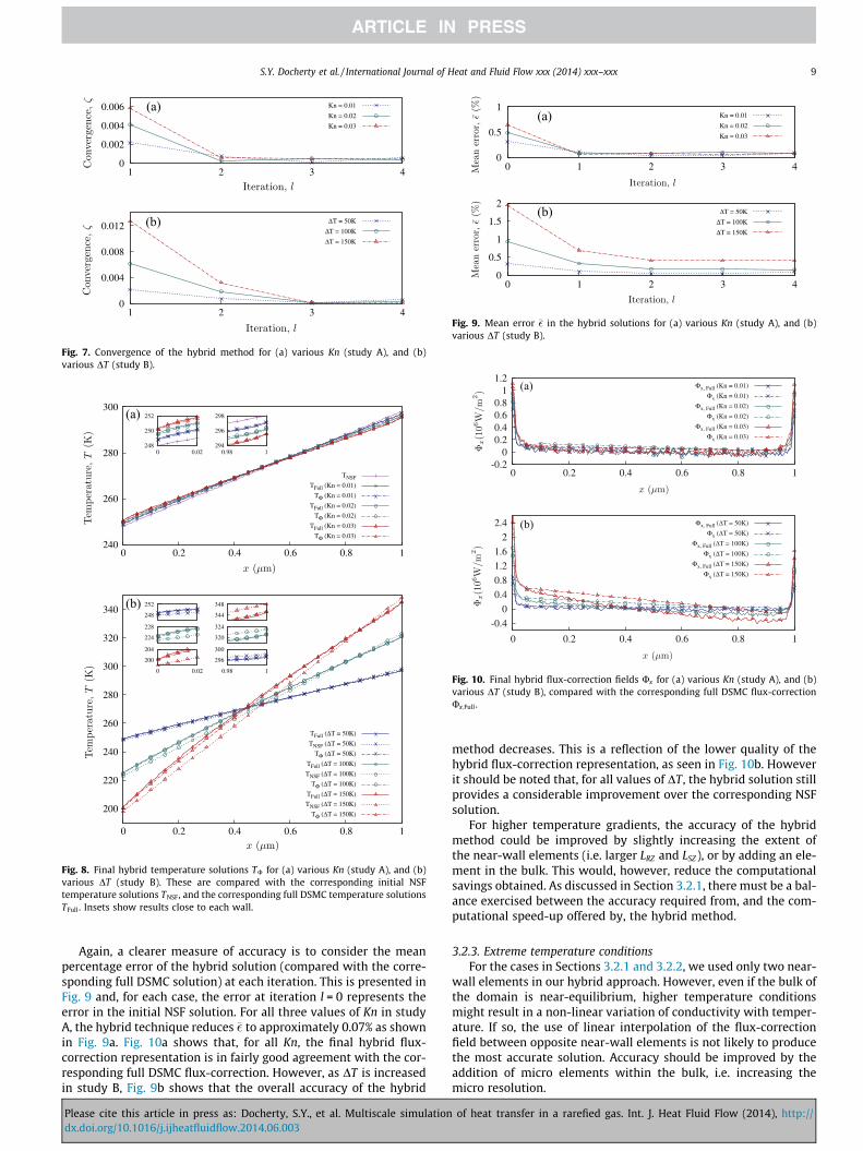
Fig. 7. Convergence of the hybrid method for (a) various Kn (study A), and (b)various DT (study B).

240

260

280

300

0 0.2 0.4 0.6 0.8 1

(a)

TNSF

TFull (Kn = 0.01)

TΦ (Kn = 0.01)

TFull (Kn = 0.02)

TΦ (Kn = 0.02)

TFull (Kn = 0.03)

TΦ (Kn = 0.03)

200

220

240

260

280

300

320

340

0 0.2 0.4 0.6 0.8 1

(b)

TFull (ΔT = 50K)

TNSF (ΔT = 50K)

TΦ (ΔT = 50K)

TFull (ΔT = 100K)

TNSF (ΔT = 100K)

TΦ (ΔT = 100K)

TFull (ΔT = 150K)

TNSF (ΔT = 150K)

TΦ (ΔT = 150K)

248

250

252

0 0.02 294

296

298

0.98 1

200

204

0 0.02

224

228

248

252

296

300

0.98 1

320

324

344

348

Fig. 8. Final hybrid temperature solutions TU for (a) various Kn (study A), and (b)various DT (study B). These are compared with the corresponding initial NSFtemperature solutions TNSF, and the corresponding full DSMC temperature solutionsTFull . Insets show results close to each wall.

0

0.5

1

0 1 2 3 4

(a) Kn = 0.01

Kn = 0.02

Kn = 0.03

0

0.5

1

1.5

2

0 1 2 3 4

(b) ΔT = 50K

ΔT = 100K

ΔT = 150K

Fig. 9. Mean error �� in the hybrid solutions for (a) various Kn (study A), and (b)various DT (study B).

-0.2 0

0.2 0.4 0.6 0.8

1 1.2

0 0.2 0.4 0.6 0.8 1

(a) Φx, Full (Kn = 0.01)

Φx (Kn = 0.01)

Φx, Full (Kn = 0.02)

Φx (Kn = 0.02)

Φx, Full (Kn = 0.03)

Φx (Kn = 0.03)

-0.4

0

0.4

0.8

1.2

1.6

2

2.4

0 0.2 0.4 0.6 0.8 1

(b) Φx, Full (ΔT = 50K)

Φx (ΔT = 50K)

Φx, Full (ΔT = 100K)

Φx (ΔT = 100K)

Φx, Full (ΔT = 150K)

Φx (ΔT = 150K)

Fig. 10. Final hybrid flux-correction fields Ux for (a) various Kn (study A), and (b)various DT (study B), compared with the corresponding full DSMC flux-correctionUx;Full.


Again, a clearer measure of accuracy is to consider the meanpercentage error of the hybrid solution (compared with the corre-sponding full DSMC solution) at each iteration. This is presented inFig. 9 and, for each case, the error at iteration l = 0 represents theerror in the initial NSF solution. For all three values of Kn in studyA, the hybrid technique reduces �� to approximately 0.07% as shownin Fig. 9a. Fig. 10a shows that, for all Kn, the final hybrid flux-correction representation is in fairly good agreement with the cor-responding full DSMC flux-correction. However, as DT is increasedin study B, Fig. 9b shows that the overall accuracy of the hybrid


method decreases. This is a reflection of the lower quality of thehybrid flux-correction representation, as seen in Fig. 10b. Howeverit should be noted that, for all values of DT , the hybrid solution stillprovides a considerable improvement over the corresponding NSFsolution.

For higher temperature gradients, the accuracy of the hybridmethod could be improved by slightly increasing the extent ofthe near-wall elements (i.e. larger LRZ and LSZ), or by adding an ele-ment in the bulk. This would, however, reduce the computationalsavings obtained. As discussed in Section 3.2.1, there must be a bal-ance exercised between the accuracy required from, and the com-putational speed-up offered by, the hybrid method.

3.2.3. Extreme temperature conditionsFor the cases in Sections 3.2.1 and 3.2.2, we used only two near-

wall elements in our hybrid approach. However, even if the bulk ofthe domain is near-equilibrium, higher temperature conditionsmight result in a non-linear variation of conductivity with temper-ature. If so, the use of linear interpolation of the flux-correctionfield between opposite near-wall elements is not likely to producethe most accurate solution. Accuracy should be improved by theaddition of micro elements within the bulk, i.e. increasing themicro resolution.




-5 0 5

10 15 20 25

0 0.2 0.4 0.6 0.8 1

Φx, Full

Φx: Π = 2

Φx: Π = 3

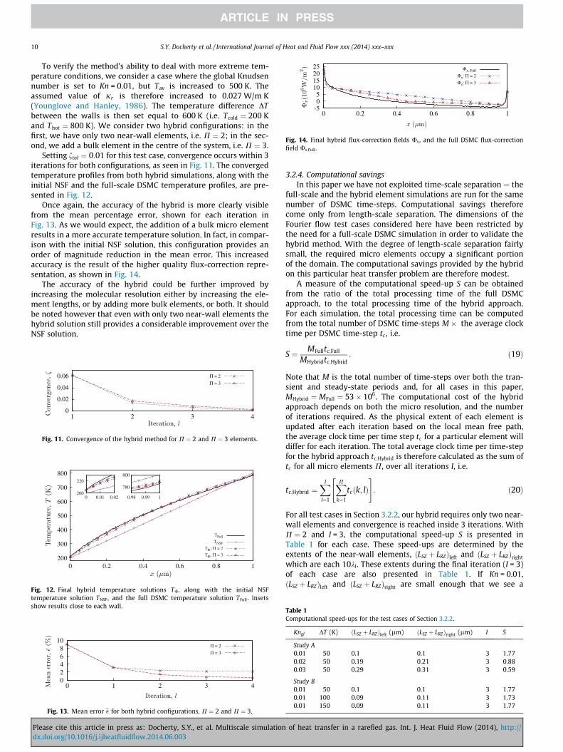
Fig. 14. Final hybrid flux-correction fields Ux , and the full DSMC flux-correctionfield Ux;Full.


To verify the method’s ability to deal with more extreme tem-perature conditions, we consider a case where the global Knudsennumber is set to Kn = 0.01, but Tav is increased to 500 K. Theassumed value of jr is therefore increased to 0.027 W/m K(Younglove and Hanley, 1986). The temperature difference DTbetween the walls is then set equal to 600 K (i.e. Tcold ¼ 200 Kand Thot ¼ 800 K). We consider two hybrid configurations: in thefirst, we have only two near-wall elements, i.e. P ¼ 2; in the sec-ond, we add a bulk element in the centre of the system, i.e. P ¼ 3.

Setting ftol ¼ 0:01 for this test case, convergence occurs within 3iterations for both configurations, as seen in Fig. 11. The convergedtemperature profiles from both hybrid simulations, along with theinitial NSF and the full-scale DSMC temperature profiles, are pre-sented in Fig. 12.

Once again, the accuracy of the hybrid is more clearly visiblefrom the mean percentage error, shown for each iteration inFig. 13. As we would expect, the addition of a bulk micro elementresults in a more accurate temperature solution. In fact, in compar-ison with the initial NSF solution, this configuration provides anorder of magnitude reduction in the mean error. This increasedaccuracy is the result of the higher quality flux-correction repre-sentation, as shown in Fig. 14.

The accuracy of the hybrid could be further improved byincreasing the molecular resolution either by increasing the ele-ment lengths, or by adding more bulk elements, or both. It shouldbe noted however that even with only two near-wall elements thehybrid solution still provides a considerable improvement over theNSF solution.

0

0.02

0.04

0.06

1 2 3 4

Π = 2

Π = 3

Fig. 11. Convergence of the hybrid method for P ¼ 2 and P ¼ 3 elements.

200

300

400

500

600

700

800

0 0.2 0.4 0.6 0.8 1

TFull

TNSF

TΦ: Π = 2

TΦ: Π = 3

200

220

0 0.01 0.02

780

800

0.98 0.99 1

Fig. 12. Final hybrid temperature solutions TU , along with the initial NSFtemperature solution TNSF, and the full DSMC temperature solution TFull . Insetsshow results close to each wall.

0 2 4 6 8

10

0 1 2 3 4

Π = 2

Π = 3

Fig. 13. Mean error �� for both hybrid configurations, P ¼ 2 and P ¼ 3.


3.2.4. Computational savingsIn this paper we have not exploited time-scale separation — the

full-scale and the hybrid element simulations are run for the samenumber of DSMC time-steps. Computational savings thereforecome only from length-scale separation. The dimensions of theFourier flow test cases considered here have been restricted bythe need for a full-scale DSMC simulation in order to validate thehybrid method. With the degree of length-scale separation fairlysmall, the required micro elements occupy a significant portionof the domain. The computational savings provided by the hybridon this particular heat transfer problem are therefore modest.

A measure of the computational speed-up S can be obtainedfrom the ratio of the total processing time of the full DSMCapproach, to the total processing time of the hybrid approach.For each simulation, the total processing time can be computedfrom the total number of DSMC time-steps M � the average clocktime per DSMC time-step tc , i.e.

S ¼ MFulltc;Full

MHybridtc;Hybrid: ð19Þ

Note that M is the total number of time-steps over both the tran-sient and steady-state periods and, for all cases in this paper,MHybrid ¼ MFull ¼ 53� 106. The computational cost of the hybridapproach depends on both the micro resolution, and the numberof iterations required. As the physical extent of each element isupdated after each iteration based on the local mean free path,the average clock time per time step tc for a particular element willdiffer for each iteration. The total average clock time per time-stepfor the hybrid approach tc;Hybrid is therefore calculated as the sum oftc for all micro elements P, over all iterations I, i.e.

tc;Hybrid ¼XI

l¼1

XPk¼1

tcðk; lÞ" #

: ð20Þ

For all test cases in Section 3.2.2, our hybrid requires only two near-wall elements and convergence is reached inside 3 iterations. WithP ¼ 2 and I = 3, the computational speed-up S is presented inTable 1 for each case. These speed-ups are determined by theextents of the near-wall elements, ðLSZ þ LRZÞleft and ðLSZ þ LRZÞright

which are each 10kl. These extents during the final iteration (I = 3)of each case are also presented in Table 1. If Kn = 0.01,ðLSZ þ LRZÞleft and ðLSZ þ LRZÞright are small enough that we see a

Table 1Computational speed-ups for the test cases of Section 3.2.2.

Kngl DT (K) ðLSZ þ LRZÞleft (lm) ðLSZ þ LRZÞright (lm) I S

Study A0.01 50 0.1 0.1 3 1.770.02 50 0.19 0.21 3 0.880.03 50 0.29 0.31 3 0.59

Study B0.01 50 0.1 0.1 3 1.770.01 100 0.09 0.11 3 1.730.01 150 0.09 0.11 3 1.77




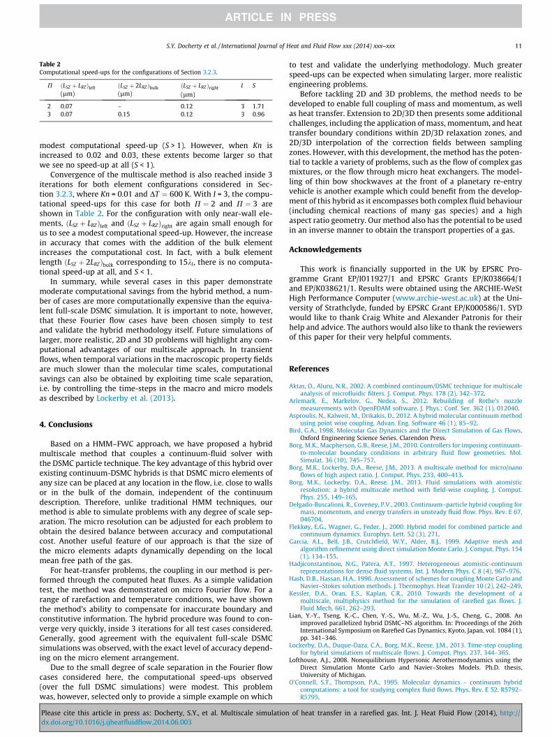
Table 2Computational speed-ups for the configurations of Section 3.2.3.

P ðLSZ þ LRZÞleft

(lm)ðLSZ þ 2LRZÞbulk

(lm)ðLSZ þ LRZÞright

(lm)I S

2 0.07 – 0.12 3 1.713 0.07 0.15 0.12 3 0.96


modest computational speed-up (S > 1). However, when Kn isincreased to 0.02 and 0.03, these extents become larger so thatwe see no speed-up at all (S < 1).

Convergence of the multiscale method is also reached inside 3iterations for both element configurations considered in Sec-tion 3.2.3, where Kn = 0.01 and DT ¼ 600 K. With I = 3, the compu-tational speed-ups for this case for both P ¼ 2 and P ¼ 3 areshown in Table 2. For the configuration with only near-wall ele-ments, ðLSZ þ LRZÞleft and ðLSZ þ LRZÞright are again small enough forus to see a modest computational speed-up. However, the increasein accuracy that comes with the addition of the bulk elementincreases the computational cost. In fact, with a bulk elementlength ðLSZ þ 2LRZÞbulk corresponding to 15kl, there is no computa-tional speed-up at all, and S < 1.

In summary, while several cases in this paper demonstratemoderate computational savings from the hybrid method, a num-ber of cases are more computationally expensive than the equiva-lent full-scale DSMC simulation. It is important to note, however,that these Fourier flow cases have been chosen simply to testand validate the hybrid methodology itself. Future simulations oflarger, more realistic, 2D and 3D problems will highlight any com-putational advantages of our multiscale approach. In transientflows, when temporal variations in the macroscopic property fieldsare much slower than the molecular time scales, computationalsavings can also be obtained by exploiting time scale separation,i.e. by controlling the time-steps in the macro and micro modelsas described by Lockerby et al. (2013).

4. Conclusions

Based on a HMM–FWC approach, we have proposed a hybridmultiscale method that couples a continuum-fluid solver withthe DSMC particle technique. The key advantage of this hybrid overexisting continuum-DSMC hybrids is that DSMC micro elements ofany size can be placed at any location in the flow, i.e. close to wallsor in the bulk of the domain, independent of the continuumdescription. Therefore, unlike traditional HMM techniques, ourmethod is able to simulate problems with any degree of scale sep-aration. The micro resolution can be adjusted for each problem toobtain the desired balance between accuracy and computationalcost. Another useful feature of our approach is that the size ofthe micro elements adapts dynamically depending on the localmean free path of the gas.

For heat-transfer problems, the coupling in our method is per-formed through the computed heat fluxes. As a simple validationtest, the method was demonstrated on micro Fourier flow. For arange of rarefaction and temperature conditions, we have shownthe method’s ability to compensate for inaccurate boundary andconstitutive information. The hybrid procedure was found to con-verge very quickly, inside 3 iterations for all test cases considered.Generally, good agreement with the equivalent full-scale DSMCsimulations was observed, with the exact level of accuracy depend-ing on the micro element arrangement.

Due to the small degree of scale separation in the Fourier flowcases considered here, the computational speed-ups observed(over the full DSMC simulations) were modest. This problemwas, however, selected only to provide a simple example on which


to test and validate the underlying methodology. Much greaterspeed-ups can be expected when simulating larger, more realisticengineering problems.

Before tackling 2D and 3D problems, the method needs to bedeveloped to enable full coupling of mass and momentum, as wellas heat transfer. Extension to 2D/3D then presents some additionalchallenges, including the application of mass, momentum, and heattransfer boundary conditions within 2D/3D relaxation zones, and2D/3D interpolation of the correction fields between samplingzones. However, with this development, the method has the poten-tial to tackle a variety of problems, such as the flow of complex gasmixtures, or the flow through micro heat exchangers. The model-ling of thin bow shockwaves at the front of a planetary re-entryvehicle is another example which could benefit from the develop-ment of this hybrid as it encompasses both complex fluid behaviour(including chemical reactions of many gas species) and a highaspect ratio geometry. Our method also has the potential to be usedin an inverse manner to obtain the transport properties of a gas.

Acknowledgements

This work is financially supported in the UK by EPSRC Pro-gramme Grant EP/I011927/1 and EPSRC Grants EP/K038664/1and EP/K038621/1. Results were obtained using the ARCHIE-WeStHigh Performance Computer (www.archie-west.ac.uk) at the Uni-versity of Strathclyde, funded by EPSRC Grant EP/K000586/1. SYDwould like to thank Craig White and Alexander Patronis for theirhelp and advice. The authors would also like to thank the reviewersof this paper for their very helpful comments.

References

Aktas, O., Aluru, N.R., 2002. A combined continuum/DSMC technique for multiscaleanalysis of microfluidic filters. J. Comput. Phys. 178 (2), 342–372.

Arlemark, E., Markelov, G., Nedea, S., 2012. Rebuilding of Rothe’s nozzlemeasurements with OpenFOAM software. J. Phys.: Conf. Ser. 362 (1), 012040.

Asproulis, N., Kalweit, M., Drikakis, D., 2012. A hybrid molecular continuum methodusing point wise coupling. Advan. Eng. Software 46 (1), 85–92.

Bird, G.A., 1998. Molecular Gas Dynamics and the Direct Simulation of Gas Flows.Oxford Engineering Science Series. Clarendon Press.

Borg, M.K., Macpherson, G.B., Reese, J.M., 2010. Controllers for imposing continuum-to-molecular boundary conditions in arbitrary fluid flow geometries. Mol.Simulat. 36 (10), 745–757.

Borg, M.K., Lockerby, D.A., Reese, J.M., 2013. A multiscale method for micro/nanoflows of high aspect ratio. J. Comput. Phys. 233, 400–413.

Borg, M.K., Lockerby, D.A., Reese, J.M., 2013. Fluid simulations with atomisticresolution: a hybrid multiscale method with field-wise coupling. J. Comput.Phys. 255, 149–165.

Delgado-Buscalioni, R., Coveney, P.V., 2003. Continuum–particle hybrid coupling formass, momentum, and energy transfers in unsteady fluid flow. Phys. Rev. E 67,046704.

Flekkøy, E.G., Wagner, G., Feder, J., 2000. Hybrid model for combined particle andcontinuum dynamics. Europhys. Lett. 52 (3), 271.

Garcia, A.L., Bell, J.B., Crutchfield, W.Y., Alder, B.J., 1999. Adaptive mesh andalgorithm refinement using direct simulation Monte Carlo. J. Comput. Phys. 154(1), 134–155.

Hadjiconstantinou, N.G., Patera, A.T., 1997. Heterogeneous atomistic-continuumrepresentations for dense fluid systems. Int. J. Modern Phys. C 8 (4), 967–976.

Hash, D.B., Hassan, H.A., 1996. Assessment of schemes for coupling Monte Carlo andNavier–Stokes solution methods. J. Thermophys. Heat Transfer 10 (2), 242–249.

Kessler, D.A., Oran, E.S., Kaplan, C.R., 2010. Towards the development of amultiscale, multiphysics method for the simulation of rarefied gas flows. J.Fluid Mech. 661, 262–293.

Lian, Y.-Y., Tseng, K.-C., Chen, Y.-S., Wu, M.-Z., Wu, J.-S., Cheng, G., 2008. Animproved parallelized hybrid DSMC–NS algorithm. In: Proceedings of the 26thInternational Symposium on Rarefied Gas Dynamics, Kyoto, Japan, vol. 1084 (1),pp. 341–346.

Lockerby, D.A., Duque-Daza, C.A., Borg, M.K., Reese, J.M., 2013. Time-step couplingfor hybrid simulations of multiscale flows. J. Comput. Phys. 237, 344–365.

Lofthouse, A.J., 2008. Nonequilibrium Hypersonic Aerothermodynamics using theDirect Simulation Monte Carlo and Navier–Stokes Models. Ph.D. thesis,University of Michigan.

O’Connell, S.T., Thompson, P.A., 1995. Molecular dynamics – continuum hybridcomputations: a tool for studying complex fluid flows. Phys. Rev. E 52, R5792–R5795.


http://www.archie-west.ac.uk

http://refhub.elsevier.com/S0142-727X(14)00083-6/h0025







































OpenFOAM Foundation, 2013. www.openfoam.org. URL <www.openfoam.org>.Patronis, A., Lockerby, D.A., Borg, M.K., Reese, J.M., 2013. Hybrid continuum–

molecular modelling of multiscale internal gas flows. J. Comput. Phys. 255, 558–571.

Ren, W., E, W., 2005. Heterogeneous multiscale method for the modeling of complexfluids and micro-fluidics. J. Comput. Phys. 204 (1), 1–26.

Roveda, R., Goldstein, D.B., Varghese, P.L., 1998. Hybrid Euler/particle approach forcontinuum/rarefied flows. J. Spacecraft Rockets 35, 258–265.

Scanlon, T.J., Roohi, E., White, C., Darbandi, M., Reese, J.M., 2010. An open source,parallel DSMC code for rarefied gas flows in arbitrary geometries. Comput.Fluids 39 (10), 2078–2089.

Schwartzentruber, T., Scalabrin, L., Boyd, I., 2007. A modular particle–continuumnumerical method for hypersonic non-equilibrium gas flows. J. Comput. Phys.225 (1), 1159–1174.

Sun, Q., Boyd, I.D., 2002. A direct simulation method for subsonic, microscale gasflows. J. Comput. Phys. 179 (2), 400–425.

Sun, Q., Boyd, I.D., Candler, G.V., 2004. A hybrid continuum/particle approach formodeling subsonic, rarefied gas flows. J. Comput. Phys. 194 (1), 256–277.

von Smoluchowski, M., 1898. Ueber wärmeleitung in verdünnten gasen. Ann. Phys.300 (1), 101–130.


Wadsworth, D.C., Erwin, D.A., 1990. One-dimensional hybrid continuum/particlesimulation approach for rarefied hypersonic flows. In: Proceedings of the 5thAIAA/ASME Joint Thermophysics and Heat Transfer Conference, Seattle, WA.

Werder, T., Walther, J.H., Koumoutsakos, P., 2005. Hybrid atomistic-continuummethod for the simulation of dense fluid flows. J. Comput. Phys. 205 (1), 373–390.

White, C., Borg, M.K., Scanlon, T.J., Reese, J.M., 2013. A DSMC investigation of gasflows in micro-channels with bends. Comput. Fluids 71, 261–271.

Wijesinghe, H.S., Hornung, R.D., Garcia, A.L., Hadjiconstantinou, N.G., 2004. Three-dimensional hybrid continuum-atomistic simulations for multiscalehydrodynamics. J. Fluids Eng. 126 (5), 768–777.

Wu, J.-S., Lian, Y.-Y., Cheng, G., Koomullil, R.P., Tseng, K.C., 2006. Development andverification of a coupled DSMC–NS scheme using unstructured mesh. J. Comput.Phys. 219 (2), 579–607.

Yasuda, S., Yamamoto, R., 2008. A model for hybrid simulations of moleculardynamics and computational fluid dynamics. Phys. Fluids 20 (11), 113101.

Younglove, B.A., Hanley, H.J.M., 1986. The viscosity and thermal conductivitycoefficients of gaseous and liquid argon. J. Phys. Chem. Ref. Data 15, 1323–1337.


http://www.openfoam.org

http://www.openfoam.org





































multiscale simulation of heat transfer in a rarefied...

Documents