multistage compression and transient flow in co pipelines
TRANSCRIPT

Multistage Compression and Transient Flow in CO2
Pipelines with Line Packing
A thesis submitted to University College London for the degree
of
Doctor of Philosophy
By
Nor Khonisah binti Daud
Department of Chemical Engineering
University College London
Torrington Place
London WC1E 7JE
March 2018

DEPARTMENT OF CHEMICAL ENGINEERING
i
I, Nor Khonisah binti Daud confirm that the work presented in this thesis is my own.
Where information has been derived from other sources, I confirm that this has been
indicated in the thesis.

DEPARTMENT OF CHEMICAL ENGINEERING
ii
Abstract
The main purpose of this thesis is to develop rigorous analytical and CFD models
followed by their applications to real case studies in order to:
i) identify the optimum multistage compression strategies for minimising the
compression and intercooler power requirements for real CO2 feed streams containing
various types and amounts of impurities associated with the various types of CO2
capture technologies;
and
ii) investigate the buffering efficacy of realistic CO2 transmission pipelines as a line
packing strategy for smoothing out temporal fluctuations in feed loading and
maintaining the desired dense-phase flow for both pure CO2 and its various realistic
mixtures representative of the most common types of capture technologies.
An analytical model based on thermodynamics principles is developed employing
Plato Silverfrost FTN95 software and applied to determine the power requirements
for various compression strategies and inter-stage cooling duties for typical pre-
combustion (98.07 % v/v of CO2) and oxy-fuel CO2 mixtures of 85 and 96.7 % v/v
CO2 purity compressed from a gaseous state at 15 bar and 38 oC to the dense-phase
fluid at 151 bar. Compression options examined include conventional multistage
integrally geared centrifugal compressors, advanced supersonic shockwave
compressors and multistage compression combined with subcritical and supercritical
liquefaction and pumping. In each case, the compression power requirement is
calculated numerically using a 15-point Gauss-Kronrod quadrature rule in
QUADPACK library, and employing the Peng-Robinson Equation of State (PR EOS)
implemented in REFPROP v.9.1 to predict the pertinent thermodynamic properties of
the CO2 and its mixtures. In the case of determining the power demand for inter-stage
cooling and liquefaction, a thermodynamic model based on Carnot refrigeration cycle
is applied. The study shows that a decrease in the impurity content from 15 to 1.9 %
v/v in the CO2 streams reduces the total compression power requirement by ca. 1.5 %
to as much as 30 %, while for all cases, inter-stage cooling duty is predicted to be

DEPARTMENT OF CHEMICAL ENGINEERING
iii
significantly higher than the compression power demand. It is found that multistage
compression combined with subcritical liquefaction using utility streams and
subsequent pumping can offer a higher efficiency than conventional integrally geared
centrifugal compression for high purity (> 96.7 % v/v) CO2 streams. In the case of a
raw/dehumidified oxy-fuel mixture, that carries a relatively large amount of
impurities (85 % v/v CO2), subcritical liquefaction at 62.53 bar is shown to increase
the cooling duty by as much 50 % as compared to that for pure CO2.
The second part of this study focuses on the development and testing of a numerical
CFD model employing Plato Silverfrost FTN95 software for simulating the transient
fluid flow behaviour in CO2 pipelines with line packing. The model is based on the
numerical solution of the conservation equations using the Method of Characteristics,
incorporating PR EOS to deal with CO2 and its various mixtures. Following its
verification, the numerical model is employed to conduct a systematic study on the
impact of operational flexibility involving a temporal reduction in the upstream CO2
feed flow rate on the transient flow behaviour in the pipe over a period of 8 hours. A
particular focus of attention is determining the optimum pipeline design and operating
line packing conditions required in order to maximise the delay in the transition from
dense phase flow to the highly undesirable two-phase flow following the ramping
down of the CO2 feed flow rate. The investigations were conducted for both pure CO2
and its various realistic mixtures. For the case studies examined, the results show that
the efficacy of line packing can be increased by increasing the pipeline length from 50
to 150 km for the same pipe inner diameter of 437 mm. However, as the pipelines
length increased to 150 km, the increase in the pipe inner diameter beyond 486 mm
was found to have no further impact on the line drafting time. While, in the case of
inlet feed temperature, the line drafting time increases following an increase in the
inlet feed temperature of transported fluid from 283.15 K up to 303.15 K. Beyond the
operating inlet feed temperature of 311.15 K, the line drafting time only marginally
increased. It is also shown that the presence of impurities reduces the transition time
to two-phase flow following the ramping down of the feed flow rate.
DEPARTMENT OF CHEMICAL ENGINEERING
iv
Impact statement
CO2 compression and transportation are essential elements in CCS which are gaining
importance in the current worldwide discussion of low carbon energy generation. The
outcome from this study intends to give future direction for research and development
in this area. The simulation results demonstrate opportunities to optimise the CCS
configuration and improve the overall economics of the power plant. These findings
also provide relevant data and act as a benchmark since its exemplify how various
industrial compression strategies can be integrated in the CCS system for typical CO2
streams captured from various capture technologies.
In the case of pipeline transportation, this work highlighted a control strategy that can
be considered during flexible operation or short-term maintenance activities to ensure
the safe operation of the high-pressure CO2 pipeline. Temporary storage or line
packing can be a useful strategy for controlling the CO2 flow in a pipeline to minimise
mass flow variations during these upset conditions. The simulation results provide a
better understanding of transport phenomena during transport of CO2 from the capture
point to the storage point of a CCS process.
This study also introduces appropriate simulation tools to determine the power
requirement for the compression processes and enable the transient analysis of CO2 in
transport pipelines. The development of analytical and numerical solution techniques
for modelling such conditions is considered as the Holy Grail by the pipeline
modellers.

DEPARTMENT OF CHEMICAL ENGINEERING
v
Publications
Impact of stream impurities on CO2 compression for Carbon Capture and
Sequestration (CCS), N.K. Daud, S. Martinov, S. Brown and H. Mahgerefteh,
ChemEngDay UK 2014, The University of Manchester, 7-8 April 2014 (Poster
Presentation).
Impact of stream impurities on CO2 compression for Carbon, Capture and
Sequestration (CCS), N.K. Daud, S. Martinov, S. Brown and H. Mahgerefteh,
UKCCSRC Biannual Meeting, University of Cardiff, 10-11th September 2014 (Poster
Presentation).
Compression Requirements for Post-Combustion, Pre-Combustion and Oxy-Fuel CO2
Streams in CCS, N.K. Daud, S. Martinov, S. Brown and H. Mahgerefteh,
International Forum on Recent Developments of CCS Implementation, Athens Ledra
Hotel, Athens, Greece, 26-27th March 2015 (Poster Presentation).
Compression Requirements for Post-Combustion, Pre-Combustion and Oxy-Fuel CO2
Streams in CCS, N.K. Daud, S. Martinov, S. Brown and H. Mahgerefteh,
ChemEngDay 2015, Sheffield, 8-9th April 2015 (Poster Presentation).
Simulation of Transient Flow in CCS Pipelines with Intermediate Storage, N.K.
Daud, S. Martynov, S. Brown and H. Mahgerefteh, 2nd International Forum on Recent
Developments of CCS Implementation, St. George Lycabettus Boutique Hotel,
Athens, Greece, 16-17th December 2015 (Poster Presentation).
Impact of stream impurities on compressor power requirements for CO2 pipeline
transportation, S.B. Martynov, N.K. Daud, H. Mahgerefteh and R.J. Porter,
International Journal of Greenhouse Gas Control, 54 (2016) 652-661.

DEPARTMENT OF CHEMICAL ENGINEERING
vi
Acknowledgements
I wish to thank the following people and organisations who have contributed so much
in many ways to facilitate the completion of this thesis.
Firstly, the Almighty God, who reigns over us. Thank you for being with me through
thick and thin.
To Ministry of Education Malaysia (MOE) and Universiti Malaysia Pahang (UMP)
for providing me with the financial resource which enabled me to complete my work.
My supervisor, Prof. Haroun Mahgerefteh for the opportunity given to me to study in
this field and your excellent supervision.
To Dr. Sergey Martynov and Zhang Wentian, for all the motivation, advice and
criticism through the course of my time at UCL.
To my family and husband, Mrs. Sopiah Binti Din and Mr. Fais Hidayat Bin Ya’amah
for their never-ending support and motivation.
Finally to all my colleagues, Rev, Jian, Dr. Richard, Ernie, Chi Ching, Sakiru, Kak
Zai, Saad, Kak Ana, Ikin, Am and Jan. Thank you for all their encouragement and
help.

DEPARTMENT OF CHEMICAL ENGINEERING
vii
Table of contents
Abstract .......................................................................................................................... ii Impact statement ........................................................................................................... iv Publications .................................................................................................................... v
Acknowledgements ....................................................................................................... vi Table of contents .......................................................................................................... vii List of figures ................................................................................................................. x List of tables ................................................................................................................. xii List of abbreviations .................................................................................................. xiii
CHAPTER 1: INTRODUCTION .................................................................................. 1
CHAPTER 2: THEORETICAL MODELLING OF MULTISTAGE COMPRESSION
POWER REQUIREMENT AND TRANSIENT FLUID FLOW .................................. 7 2.0 Introduction .............................................................................................................. 7 2.1 Modelling of multistage compression power requirement ...................................... 7
2.1.1 Compression model .............................................................................................. 8
2.1.2 Compressor efficiency ........................................................................................ 10
2.1.3 Multistage compression with intercooling .......................................................... 11
2.1.4 Compression pressure ratio ................................................................................. 14
2.1.5 Intercooling heat ................................................................................................. 16
2.1.6 Properties of CO2 mixtures with impurities ........................................................ 16
2.2 Application of the compression model .................................................................. 19
2.2.1 Witkowski and Majkut (2012) and Witkowski et al. (2013) .............................. 19
2.2.2 Pei et al. (2014) ................................................................................................... 24
2.2.3 Romeo et al. (2009)............................................................................................. 25
2.2.4 Moore et al. (2011) ............................................................................................. 26
2.2.5 Duan et al. (2013) ............................................................................................... 27
2.2.6 Modekurti et al. (2017) ....................................................................................... 31
2.2.7 Aspelund and Jordal (2007) ................................................................................ 33
2.2.8 de Visser et al. (2008) ......................................................................................... 35
2.2.9 Goos et al. (2011) ................................................................................................ 35
2.2.10 Chaczykowski and Osiadacz (2012) ................................................................. 36 2.3 Concluding remarks ............................................................................................... 37
2.4 Modelling of transient fluid flow in pipelines ....................................................... 38
2.4.1 Model assumptions ............................................................................................. 41
2.4.2 Conservation of mass .......................................................................................... 42
2.4.3 Conservation of momentum ................................................................................ 45
2.4.4 Conservation of energy ....................................................................................... 46
2.4.5 Thermodynamic analysis .................................................................................... 49
2.4.6 Hydrodynamic analysis ....................................................................................... 53
2.4.7 Numerical methods for the solution of transient fluid flow model ..................... 56 2.5 Application of the transient fluid flow model ........................................................ 66
2.5.1 OLGA ................................................................................................................. 67
2.5.2 University College London (UCL) model .......................................................... 70

DEPARTMENT OF CHEMICAL ENGINEERING
viii
2.5.3 SLURP ................................................................................................................ 74
2.5.4 Terenzi ................................................................................................................ 78
2.5.5 Popescu ............................................................................................................... 80 2.6 Concluding remarks ............................................................................................... 82
CHAPTER 3: STUDY OF MULTISTAGE COMPRESSION OF CO2 WITH
IMPURITIES FOR CCS .............................................................................................. 83 3.0 Introduction ............................................................................................................ 83
3.1 Technical background ............................................................................................ 83 3.2 CO2 stream impurities ............................................................................................ 87
3.2.1 Oxy-fuel combustion capture .............................................................................. 89
3.2.2 Pre-combustion capture ...................................................................................... 89
3.2.3 Post-combustion capture ..................................................................................... 90
3.2.4 Impact of impurities on CO2 physical properties ................................................ 90
3.3 Industrial compression technologies ...................................................................... 94
3.3.1 Option A: Conventional multistage integrally geared centrifugal compressors . 95
3.3.2 Option B: Advanced Supersonic Shockwave Compression ............................... 98
3.3.3 Option C: Multistage compression combined with subcritical liquefaction and
pumping ....................................................................................................................... 99
3.3.4 Option D: Multistage compression combined with supercritical liquefaction and
pumping ..................................................................................................................... 101 3.4 Methodology: Thermodynamic analysis.............................................................. 102
3.5 Properties of CO2 mixtures with impurities ......................................................... 104 3.6 Results and Discussions: Multistage compression of CO2 streams containing
impurities ................................................................................................................... 106
3.6.1 Multistage compression of an impure CO2 stream ........................................... 109
3.6.2 Multistage compression power demands .......................................................... 118
3.7 Conclusions .......................................................................................................... 125
CHAPTER 4: TRANSIENT FLOW MODELLING IN CO2 PIPELINES DURING
LINE PACKING AND LINE DRAFTING ............................................................... 129 4.0 Introduction .......................................................................................................... 129
4.1 Factors that influence the operating flexibility of power plants as part of CCS .. 131
4.1.1 Constant flow of CO2 to transport and storage ................................................. 135
4.2 Numerical pipe flow model ................................................................................. 139
4.2.1 Governing equations ......................................................................................... 139
4.2.2 Boundary conditions ......................................................................................... 140
4.2.3 Numerical method ............................................................................................. 144 4.3 Analytical model .................................................................................................. 145
4.4 Results and discussion ......................................................................................... 146
4.4.1 Effect of operational flexibility on pipeline flow ............................................. 146
4.4.2 Optimal parameter investigation for avoiding two-phase flow during flexible
operation .................................................................................................................... 158
4.4.3 Application of the optimised line packing parameters ................................... 162
CHAPTER 5: CONCLUSIONS AND RECOMMENDATIONS FOR FUTURE
WORK ....................................................................................................................... 166
5.1 Conclusions .......................................................................................................... 166
5.2 Recommendations for future work ...................................................................... 172 References .................................................................................................................. 174

DEPARTMENT OF CHEMICAL ENGINEERING
ix
Appendix A: Multistage compression (Fortran Plato IDE) ....................................... 187 Appendix B: Line Packing ......................................................................................... 192
Appendix C: Analytical method (Fotran Plato IDE) ................................................. 216

DEPARTMENT OF CHEMICAL ENGINEERING
x
List of figures
Figure 2.1: Compression power as function of compressor isentropic efficiency
(Austbø, 2015). ............................................................................................................ 11
Figure 2.2: Two-stage compression with intercooling (Austbø, 2015). ...................... 12
Figure 2.3: A P-h diagram for two-stage compressor with an intercooler (Wu et al.,
1982). ........................................................................................................................... 12
Figure 2.4: Comparison of the energy savings in two-stage compression with
intercooling with different pressure ratio (Austbø, 2015). .......................................... 15
Figure 2.5: Compression work and total work consumption for different CO2
compression scenarios (Duan et al., 2013). ................................................................. 29
Figure 2.6: Variation of energy requirement for P1, P2 and S1 as a function of inlet
pressure (Aspelund and Jordal, 2007). ......................................................................... 34
Figure 2.7: Variation of energy requirement for P1, P2 and S1 as a function of inert
gas content (Aspelund and Jordal, 2007). .................................................................... 34
Figure 2.8: Variation of compressor station power (Chaczykowski and Osiadacz,
2012). ........................................................................................................................... 36
Figure 2.9: A schematic representation of flow and space variables of a representative
pipeline to the vertical and horizontal planes (Bratland, 2009). .................................. 42
Figure 2.10: A schematic representation of Path line (C0) and Mach lines (C+, C-)
characteristics at a grid point along the time, t and space, x axis. ............................... 60
Figure 2.11: The Characteristic grid (Wylie et al., 1971). ........................................... 61
Figure 2.12: The method of Specified Time Intervals (Wylie et al., 1971). ................ 62
Figure 2.13: Comparison of the field test data with the OLGA simulation result during
slow blowdown scenario (Shoup et al., 1998). ............................................................ 68
Figure 2.14: Comparison of the field test data with the OLGA simulation result during
rapid blowdown scenario (Shoup et al., 1998). ........................................................... 68
Figure 2.15: Comparison between OLGA and experimental data for case 2 at P14,
P19 and P24 (Botros et al., 2007). ............................................................................... 69
Figure 2.16: Intact end pressure vs. time profiles for the Piper Alpha to MCP pipeline
(Mahgerefteh et al., 1999). ........................................................................................... 71
Figure 2.17: FBR pressure vs. time profiles at the open end for test P40 (LPG)
showing the effect of primitive variables on simulated results (Oke et al., 2003). ..... 73
Figure 2.18: Pressure vs. time profiles at open end for test P40 (LPG) (Mahgerefteh et
al., 2007). ..................................................................................................................... 74
DEPARTMENT OF CHEMICAL ENGINEERING
xi
Figure 2.19: Comparison between SLURP model and measured variation of pipeline
inventory with time for test T61 (Cleaver et al., 2003). .............................................. 76
Figure 2.20: Comparison between SLURP model and measured variation of pipeline
inventory with time for test T63 (Cleaver et al., 2003). .............................................. 76
Figure 2.21: Comparison between SLURP model and measured variation of pipeline
inventory with time for test T65 (Cleaver et al., 2003). .............................................. 77
Figure 2.22: Comparison of predicted release rate for a propane pipeline at an initial
pressure of 46 bara and 15 oC (Cumber, 2007). ........................................................... 78
Figure 2.23: Measured and calculated decompression wave speed results of NABT
Test 5 (Picard and Bishnoi, 1987)................................................................................ 79
Figure 2.24: Comparison of the variation of pressure with time between predicted and
experimental for a 11.5 m pipeline containing methane (Popescu, 2009). .................. 81
Figure 2.25: Comparison of the variation of pressure with time between predicted and
experimental for a 34.5 m pipeline containing hydrogen (Popescu, 2009). ................ 81

DEPARTMENT OF CHEMICAL ENGINEERING
xii
List of tables
Table 2.1: Comparison of compression technology options (Witkowski and Majkut,
2012). ........................................................................................................................... 21
Table 2.2: Options CS1 and CS2 (Witkowski and Majkut, 2012). ............................... 22
Table 2.3: Summary of compression and pumping power reduction (Witkowski and
Majkut, 2012). .............................................................................................................. 23
Table 2.4: Performance of intercooling compression coupled with ORC (Pei et al.,
2014). ........................................................................................................................... 24
Table 2.5: Performance of 2-stage shockwave compression coupled with ORC (Pei et
al., 2014). ..................................................................................................................... 24
Table 2.6: Performance data of different CO2 compression and liquefaction processes
(Duan et al., 2013). ...................................................................................................... 28
Table 2.7: The comparison results of different CO2 compression methods (Duan et al.,
2013). ........................................................................................................................... 30
Table 2.8: Compressor comparison summary (Modekurti et al., 2017). .................... 32
Table 2.9: Comparison of the specific compression power for different CO2 gas
mixtures compressed to 110 bar (Goos et al., 2011).................................................... 35
Table 2.10: Subset of tests from the Isle of Grain experiments used in the validation of
SLURP (Cleaver et al., 2003). ..................................................................................... 75
Table 2.11: Failure scenarios used in the comparison of predicted outflow calculated
using SLURP and PROFES for a pipeline at an initial temperature of 15 oC containing
carrying an inventory of 100 % propane (Cumber, 2007). .......................................... 77

DEPARTMENT OF CHEMICAL ENGINEERING
xiii
List of abbreviations
CCS Carbon Capture and Sequestration
CO2 Carbon Dioxide
CFD Computational Fluid Dynamics
MW Megawatt
PR EOS Peng-Robinson Equation of State
MOC Method of Characteristics
REFPROP Reference Fluid Thermodynamic and Transport Properties
Database
kW Kilowatt
ORC Organic Rankine Cycle
COE Cost of Electricity
TEG Triethylene Glycol
LHS Left Hand Side
RHS Right Hand Side
GERG Groupe Européen de Recherches Gazières
VLE Vapour Liquid Equilibrium
LK Lee-Kesler
SAFT Statistical Associating Fluid Theory
RK Redlich-Kwong
SRK Soave-Redlich-Kwong
PT Patel-Teja
AAD Absolute Average Deviation
FDM Finite Difference Methods
FVM Finite Volume Methods
PDE Partial Differential Equation
CG Characteristic Grid
MST Method of Specified Time Intervals
ODE Ordinary Differential Equation
CFL Courant-Friedrichs-Lewy
OLGA Oil and Gas Simulator
GDTF Gas Dynamic Test Facility
HEM Homogeneous Equilibrium Mixture Model
CNGS-MOC Compound Nested Grid System Method of Characteristics
PDU Pressure, density and velocity
PHU Pressure, enthalpy and velocity
PSU Pressure, entropy and velocity
COSTALD Corresponding State Liquid Density
PROFES Probabilistic Finite Element System
IGCC Integrated Gasification Combine Cycle
ASU Air Separation Unit
AGR Acid Gas Recovery
QUADPACK A Subroutine Package for Automatic Integration
ANN Artificial Neural Network
RES Renewable Energy Resources
PC Pulverised Coal

DEPARTMENT OF CHEMICAL ENGINEERING
xiv
IGCC Integrated Gasification Combine Cycle
NGCC Natural Gas Combine Cycle
CCGT Combine Cycle Gas Turbine
LOX Liquid Oxygen
AGRU Acid Gas Removal Unit
MAOP Maximum Allowable Operating Pressure
ISO Independent System Operator

DEPARTMENT OF CHEMICAL ENGINEERING
1
CHAPTER 1:
INTRODUCTION
Carbon Capture and Sequestration (CCS) has been proposed as a promising
technology to mitigate the impact of anthropogenic CO2 emissions from the
manufacturing industry and power generation sources, such as coal-burning power
plants, on global warming (Metz et al., 2005). A fundamental part of the CCS chain is
the transportation of CO2 captured from emitters to locations of geological
sequestration. Long-distance onshore and offshore transportation of large quantities of
CO2 can be efficiently achieved using pipelines transmitting CO2 in the dense phase at
pressures typically above 86 bar (McCoy and Rubin, ), i.e. above the fluid
critical point pressure (Seevam et al., 2008, Yoo et al., 2013). Given the relatively low
pressure of captured CO2 (Pei et al., 2014), the pipeline transportation requires
additional facilities for compression of the stream which can be extremely energy
intensive and hence expensive.
Compression of captured CO2 to the high pressures suitable for transportation can be
accompanied by a significant temperature rise, typically above 100 oC. Such high
temperatures can damage the compressor and pipeline internal coatings employed to
reduce pipeline degradation. Therefore, cooling is applied during compression and
before the pipeline transportation of the CO2 stream. The cost of CO2 compression is
however significant, and may be up to 8-12 % of the electricity generated from the
power plant (Moore et al., 2011). In addition, the available conventional CO2
compression systems are prohibitively expensive due to the high overall pressure ratio
(e.g. 100:1) used. The above highlight the necessity for detailed analysis in order to
minimise both compressor power and capital cost requirements of the compression
system. Several options have been recently analysed in the literature for compression
of CO2 for transportation in pipelines (Witkowski and Majkut, 2012). These options
include those using conventional multistage centrifugal compressors, compressors
combined with subcritical and supercritical liquefaction and pumping, and supersonic
axial compressors. Among these options, the multistage compression combined with

DEPARTMENT OF CHEMICAL ENGINEERING
2
liquefaction and pumping has been reported to be the most efficient (Witkowski and
Majkut, 2012). This option is practically attractive since the pumping of a liquid is
less energy demanding than gas-phase compression, while relatively high boiling of
pure CO₂ point (ca. 20 oC at 60 bar) allows using utility streams for the liquefaction
process. Supersonic shock-wave compressors can be used for the compression of
large amounts of fluid, having lower capital costs than traditional centrifugal
compressors.
In the case of industrial-grade CO₂, the presence of any impurities is expected to
diminish the net amount of CO₂ processed, and hence reduce the efficiency of the
entire CCS operation. However, once the stream is purified to an acceptable level for
pipeline transport and geological storage, it is important to identify the compression
strategy giving rise to the lowest cost for the particular CO₂ composition. The choice
of the compression strategy and costs associated with compression depend on the
physical properties of the CO₂ mixture, such as fluid compressibility, density and
saturation temperature and pressure. For example, when using multistage compression
combined with liquefaction, the variation of the fluid boiling point with the CO₂
stream composition will have a direct impact on the liquefaction pressure and, hence,
the efficiency of the compression process. At present, however, the qualitative impact
of CO₂ stream impurities on the power requirements and choice of the optimum
compression strategy remains unclear.
For these reasons, the development of efficient schemes for the compression and
conditioning of CO2 prior to its transportation by pipeline, and integration of these
schemes within CCS, is an important practical issue, which is attracting increasing
attention (Ludtke, 2004, Romeo et al., 2009, Moore et al., 2011, Witkowski and
Majkut, 2012). However, the selection and development of optimal compression
strategies are particularly dependent on the type of the CO2 separation technology
employed. In a typical post-combustion capture, nearly pure CO2 stream is separated
from the flue gas stream close to ambient pressure, while in pre-combustion and oxy-
fuel captures, ca. 15-30 bar separation pressures are applied (Witkowski and Majkut,
2012, Besong et al., 2013), with ‘double flash’ or distillation cryogenic separation

DEPARTMENT OF CHEMICAL ENGINEERING
3
methods commonly proposed for the removal of non-condensables (e.g. N2, O2 and
Ar).
Oxy-fuel is one of the capture technologies which has recently gained significant
attention due to its eligibility for retrofitting and CCS-ready concepts. However,
compared to the more traditional post-combustion and pre-combustion capture
technologies, oxy-fuel technology produces a raw CO2 stream with relatively high
concentration of impurities that may require partial or a high level of removal and
whose presence can be expected to increase the costs of CO2 compression and
pipeline transportation compared to pure CO2. Since CO2 compression systems are
commonly designed assuming negligible amount of impurities in the CO2 fluid, it is
of practical interest to evaluate the impact of impurities in pre-combustion and oxy-
fuel streams on the compression power requirements.
Therefore, this study is motivated by the need to gain a better understanding of the
possibilities and limitations of the impure CO2 compression process for oxy-fuel and
pre-combustion capture applications. An investigation into the efficient transportation
of CO2 during flexible operation is the second purpose of this study. The existing
commercial application of CO2 pipelines is based on ‘base-load operation’, i.e. no
significant temporal variations in the feed rate is envisaged (IEAGHG, 2012). In
practice however, depending on the CO2 emission source, variations in the CO2 feed
flow rate, for example during uncertain electricity supply and demand from fossil fuel
power plants will be inevitable. Hence in these circumstances designing a self-
regulating CO2 pipeline transport system enabling the steady flow delivery of CO2 to
the sequestration sites becomes important.
Chalmers and Gibbins (2007) suggest that any restrictions on short-term operating
patterns can be avoided by adopting operating procedures that allow for some CO2
buffering in the pipeline transportation system. The use of a pipeline as short-term
storage is an appropriate strategy to ensure the fluctuation of the flow in the pipeline
system can be minimised. This strategy is defined as ‘line-packing’ where the pipeline
pressure is varied to pack more or less CO2 by employing the pipeline as storage
vessel (Jensen et al., 2016b).

DEPARTMENT OF CHEMICAL ENGINEERING
4
Some works have been carried out on the dynamics of CO2 transport pipeline systems
(Liljemark et al., 2011, Klinkby et al., 2011, Mechleri et al., 2016, Aghajani et al.,
2017). These findings lend support and provide guidelines to investigate the flexibility
in the pipeline system by employing the pipe as short-term storage. In order to
investigate the efficacy of this method, the stored CO2 is de-packed or drafted to
supply the needs during periods of significant load fluctuation to maintain the flow
into the pipeline and sequestration site. In pipeline terminology, increasing the
inventory is called line packing, while decreasing it is called line drafting (de Nevers
and Day, 1983). The time available to under-take line drafting is called the line-
drafting time. In this study, the flexibility to line-draft a pipeline is assessed by
determining the time available for an operator to de-pack dense phase CO2 in the
pipeline during flexible operations.
The optimum parameters selection for line packing is investigated by studying the
impact of pipeline design parameters, inlet mass flow rate and inlet temperature on the
available line drafting time. The selection of the range of pipeline dimensions in terms
of length, diameter and wall thickness is based on the design criterion outlined in
McCoy and Rubin () and Aghajani et al. (2017). The efficacy of the optimised
line packing is investigated by studying the impact of impurities on the line drafting
time, the CO2 mixtures captured from pre-combustion and oxy-fuel capture
technologies are employed based on the compression case study. In particular, these
impurities have a significant impact on the physical properties of the transported CO2
which make it difficult to maintain the single-phase flow. The presence of impurities
also affect pipeline resistance to fracture propagation, corrosion, non-metallic
deterioration, the formation of clathrates and hydrates as well as changing the
capacity of the pipeline itself (Seevam et al., 2008, Jensen et al., 2016b). All these
effects have direct implications for both the technical and economic feasibility of
designing an efficient CO2 pipeline transport.
Therefore, the main purpose of this study is to develop mathematical models to:

DEPARTMENT OF CHEMICAL ENGINEERING
5
i) identify the optimum multistage compression strategies for minimising
compression power consumption for real CO2 feed streams containing various
types and amounts of impurities;
and
ii) investigate the buffering efficacy of realistic CO2 transmission pipelines as a
strategy for smoothing out temporal fluctuations in feed loading associated
with typical emission sources.
Hence, the main objectives of this study are:
1. To develop a rigorous mathematical model for multistage compression of pure
and impure CO2 streams captured from pre-combustion and oxy-fuel capture
technologies as well as to determine and compare the corresponding
compression power requirements.
2. To determine the optimum multistage compression strategies in order to
minimise the power requirements in the compression system.
3. To develop a transient pipeline flow model to simulate feed load ramping
during flexible operation.
4. Use the transient flow model developed above to investigate the impacts of
pipeline overall dimensions, inlet fluid temperature, inlet mass flow rate and
CO2 impurities on the efficacy of a pipeline as line packing.
This thesis is divided into 5 chapters:
In chapter 2, the theoretical basis for calculating the compression power and
intercooling heat in a multistage compression system are presented and discussed. The
general equations to calculate the compression power and thermodynamics properties
are derived and explained. The implementation of these equations from the previous
reported studies are also reviewed in the following section. This chapter also covers
the theoretical basis in developing the pipeline flow model for dense phase CO2
streams together with its assumptions and justifications. The mass, momentum and
energy conservation equations for the fluid flow in the pipeline system are presented.

DEPARTMENT OF CHEMICAL ENGINEERING
6
The numerical methods used for solving the conservation equations including the
method of characteristics (MOC) are discussed. The mathematical models available in
the open literature for simulating the transient flow in the high-pressure CO2 pipeline
system are also reviewed in this chapter.
Chapter 3 covers the description of the types of industrial compression technologies
employed and the impurities present in the pre-combustion and oxy-fuel streams. This
section also presents a description of the rigorous thermodynamic model developed to
determine the total power consumption for multistage compression of pure and
impure captured CO2 streams. From the developed mathematical model, the optimum
multistage compression schemes are determined depending on the outlet pressure
from the separation unit of the captured streams and the thermodynamic properties of
the CO2 mixtures. The calculated power requirements for compression and
intercooling heat for various compression schemes for particular CO2 mixtures are
compared and discussed.
In chapter 4, the influence of line packing on maintaining the near-steady flow
condition for pure and impure CO2 during flexible operation is discussed. The
development of the numerical transient pipe flow model and simplified analytical
model are presented, including the governing conservation equations, the boundary
conditions and the solution method. Steady state flow is established in the pipeline
before the transient feed loadings are mimicked by gradually closing a feed valve at
the upstream of the pipe. The effect of operational flexibility on pipe is investigated
accounting for impurities components. The validity of the simplified analytical model
is studied against developed transient pipe flow model. A number of hypothetical but
nevertheless realistic flexible loading scenarios are simulated in order to demonstrate
the robustness and the efficacy of the flow model as a control design and operation
tool. The impact of pipeline overall dimensions, inlet temperature, inlet mass flow
rate and CO2 impurities on the line drafting time are simulated and the results are
discussed. Chapter 5 summarises the key outcomes of the study and suggestions for
future research.

DEPARTMENT OF CHEMICAL ENGINEERING
7
CHAPTER 2:
THEORETICAL MODELLING OF MULTISTAGE
COMPRESSION POWER REQUIREMENT AND TRANSIENT
FLUID FLOW
2.0 Introduction
In this chapter, the theoretical bases for calculating the compression power and
intercooling heat exchanges in a multistage compression system are presented. The
general equations to calculate the compression power and thermodynamics properties
are discussed. The implementation of these equations from the previous reported
studies are also reviewed. This chapter also covers the theoretical basis for modelling
the transient fluid flow in the high-pressure CO2 pipeline together with its
assumptions and justifications. The mass, momentum and energy conservation
equations for the fluid flow in the pipeline system are also presented. The numerical
methods used for solving the conservation equations in particular the Method of
Characteristics (MOC) are discussed. The mathematical models available in the open
literature for simulating the transient flow in the high-pressure CO2 pipeline system
are also reviewed in this chapter as a prelude to the next chapter dealing with the
pressure and flow fluctuations during load change.
2.1 Modelling of multistage compression power requirement
This section deals with the general equations to determine the total power
consumption for multistage compression system equipped with intercooling
equipment. Fundamentally, these equations are derived from basic thermodynamic
and energy balance relations.

DEPARTMENT OF CHEMICAL ENGINEERING
8
2.1.1 Compression model
The compression work, compW for isentropic, polytropic and isothermal processes
between pressure levels, P1 and P2, based on ideal gas assumption are respectively
given by (Cengel and Boles, 2011),
Isentropic ( PV = constant):
11
1
1
21
P
PRTWcomp
2.1
Polytropic (PVn = constant):
11
1
1
21
n
n
compP
PRT
n
nW 2.2
Isothermal (PV = constant):
1
2lnP
PRTWcomp 2.3
where P, V, R, T, and n are the pressure, volume of the fluid, universal gas
constant, fluid temperature and the isentropic as well as polytropic exponents,
respectively. The subscripts 1 and 2 indicate the conditions at the suction and
discharge of the compressor.
The equations 2.1-2.3 are appropriate for the calculation and analysis of an ideal gas.
In the case of a real gas such as CO2, from the general energy balance relations
(Cengel and Boles, 2011),
in E mass, and work heat,by
innsfer energy tranet of Rate =
out E mass, and work heat,by
out nsfer energy tranet of Rate 2.4

DEPARTMENT OF CHEMICAL ENGINEERING
9
Noting that energy can be transferred by heat, work and mass only, the energy balance
in equation 2.4 for a general steady-flow system can also be written more explicitly as
(Cengel and Boles, 2011):
gz
vhmWQgz
vhmWQ
out
outout
in
inin22
22
2.5
where h, v, z and g are the fluid enthalpy, velocity, height and gravity, respectively.
inQ , inW and inm are the heat transferred, total work and mass flow rate into the
system, while outQ , outW and outm are the heat transferred, total work and mass flow
rate out of the system.
Compressors are devices used to increase the pressure of a fluid. Work is supplied to
this device from an external source through a rotating shaft. Therefore, compressors
involve work inputs at a rate of W, while heat is assumed to be transferred from the
system (heat output) and at a rate of Q. Thus, the energy balance relation for a general
steady-flow system becomes:
inout
gzv
hmgzv
hmQW22
22
2.6
For single-stream devices, the steady flow energy balance equation 2.6 becomes:
12
2
1
2
212
2zzg
vvhhmQW 2.7
In the case of the compressor, the fluid experiences negligible changes in its kinetic
and potential energies. The velocities involved are usually too low to cause any
significant change in the kinetic energy. This change is usually very small relative to
the change in enthalpy, and thus it is often disregarded. Heat transfer from
compressors is usually negligible 0Q since they are typically well insulated
unless there is intentional cooling. The energy balance equation (equation 2.7) is thus
reduced further to:
DEPARTMENT OF CHEMICAL ENGINEERING
10
12 hhmWcomp 2.8
where m, h1 and h2 are the mass flow rate, suction and discharge enthalpies,
respectively. Thus, the compression work of a single compressor for a real gas fluid
can be determined using equation 2.8.
2.1.2 Compressor efficiency
Compression system analysis is often carried out assuming a constant isentropic
efficiency for compressors. The isentropic compression system is impossible in
reality. However, for the simplification of the calculation, the isentropic efficiency is
employed because it can be directly derived from the station design parameters, i.e.
gas composition, suction temperature and pressure as well as discharge pressure.
Whereas, the definition of polytropic efficiency requires the additional knowledge of
the discharge temperature of the compression system. The isentropic efficiency of a
compression process can be defined as:
a
s
a
scompis
h
h
W
W
, 2.9
where sW , aW , sh and ah are the compression work of an isentropic process, the
actual compression work, the specific enthalpy change in an isentropic process and
the specific enthalpy change of the actual process, respectively. In any real process,
the isentropic efficiency is smaller than unity (Austbø, 2015).
The effect of the compressor isentropic efficiency on the compression work can be
presented in figure 2.1.

DEPARTMENT OF CHEMICAL ENGINEERING
11
Figure 2.1: Compression power as function of compressor isentropic efficiency
(Austbø, 2015).
As can be observed in figure 2.1, the compression work decreases with increasing
isentropic efficiency. Also, larger absolute savings in power consumption are obtained
when the efficiency is high.
In order to calculate the compression work (equation 2.8) for a real gas, the discharge
enthalpy, h2 can be determined using isentropic efficiency, compis, of the compressor,
compis
is hhhh
,
12,
12
2.10
where 2,ish is the discharge enthalpy for the isentropic process.
The value of compis, greatly depends on the design of the compressor. Well-designed
compressors have isentropic efficiencies that range from 80 to 90 % (Cengel and
Boles, 2011).
2.1.3 Multistage compression with intercooling
Multistage compression with intercooling is an efficient means for reducing power
consumption. It is clear that cooling a gas as it is compressed is desirable since this
reduces the required work input to the compressor and avoids damage to the
compressor seals due to high temperatures. However, often it is not possible to have
adequate cooling through the casing of compressor, and it becomes necessary to use
other techniques to achieve effective cooling. One such technique is multistage

DEPARTMENT OF CHEMICAL ENGINEERING
12
compression with intercooling, where the gas is compressed in stages and cooled
between each stage by passing it through a heat exchanger called an intercooler as
shown in figure 2.2.
Figure 2.2: Two-stage compression with intercooling (Austbø, 2015).
Ideally, the cooling process takes place at constant pressure, and the gas is cooled to
the initial temperature at each intercooler. Multistage compression with intercooling is
especially attractive when a gas is to be compressed to very high pressures.
The effect of intercooling on compressor work is illustrated on P-h diagram in figure
2.3 for a two-stage compressor, where P1 and P3 are the suction pressure and
discharge pressure, respectively.
Figure 2.3: A P-h diagram for two-stage compressor with an intercooler (Wu et al.,
1982).

DEPARTMENT OF CHEMICAL ENGINEERING
13
The compression work, Wcomp,1 of the single isentropic compressor equals the specific
enthalpy difference between point 3 and point 1 multiplied by the mass flow rate, m
of the gas and can be expressed as:
)( 131, hhmWcomp 2.11
If two-stage compression is used instead of one-stage compression, and the
assumption is made that there is no pressure drop in the intercooler, the overall
compressive process curve is presented by the paths 1-2-4-5 in figure 2.3. The gas is
compressed in the first stage from P1 to an intermediate pressure P2 at point 2, cooled
at constant pressure at point 4 and compressed in the second stage to the final
pressure, P3 at point 5. The area in the process curve 2-3-4-5 on the P-h diagram
represents the work saved as a result of two-stage compression with intercooling. The
size of the saved work varies with the value of the intermediate pressure and it is of
practical interest to determine the conditions under which this area is maximised. The
total compression work for a two-stage compressor is the sum of the work inputs for
each stage of compression, as determined from:
4512
'
2, hhmhhmWcomp 2.12
Since the slope of the process curve 4-5 is larger than the slope of the curve 1-3 and
the pressure limits are equal, then,
2345 hhhh 2.13
The compression work saved by using this ideal intercooler is:
4523
' hhmhhmW 2.14
In fact, there is pressure drop in a non-ideal intercooler, thus, the pressure of gas at the
outlet of the intercooler is P6, less than P4. The total compression work for the two-
stage compressor, 2,compW then equals
67122, hhmhhmWcomp 2.15
The actual compression work saved is given as:

DEPARTMENT OF CHEMICAL ENGINEERING
14
6723 hhmhhmW 2.16
ΔW is less than ΔW’ because 64 hh and 57 hh . Theoretically, the higher the heat
transfer rate of the intercooler, the lower the temperature at point 6 will be and the
greater the quantity of energy can be saved. But it is impossible to remove too much
heat from gas to water because of the cost limitation of the intercooler (Wu et al.,
1982).
2.1.4 Compression pressure ratio
The intermediate pressure value, P2 as shown in figure 2.2, that minimises the total
work is determined by introducing the compression pressure ratio terms. The
compression pressure ratios, PR for compressors A (COMP-A) and B (COMP-B) (see
figure 2.2) are defined as:
2
3
1
2
P
PPR
P
PPR
BCOMP
ACOMP
2.17
where 2P and 1P are the discharge and suction pressures of the compressor A, while
3P and 2P are the discharge and suction pressures of the compressor B, respectively.
An acceptable compression pressure ratio for centrifugal compressors is ca. 1.5 to 2
(Menon, 2005). A larger number requires more compressor power. If the number of
stages of compressor is installed in series to achieve the required compression
pressure ratio, then each compressor stage can be operated at a compression pressure
ratio of (Menon, 2005),
NtPRPR
1
2.18
where PRt and N are the overall compression pressure ratio and the number of
compressor stages in series respectively.

DEPARTMENT OF CHEMICAL ENGINEERING
15
Figure 2.4 shows the comparison of the energy savings in the two-stage compression
with different compression pressure ratio, PR where T1 and T3 are the initial gas
temperature at the inlet first compressor and the gas temperature after cooling from
the first intercooler (see figure 2.2) respectively.
Figure 2.4: Comparison of the energy savings in two-stage compression with
intercooling with different pressure ratio (Austbø, 2015).
With increasing pressure ratio, the peak in energy savings is moved to a larger value
of T3 − T1. Since the overall pressure ratio is larger, so is the discharge temperatures
of the compressors. The isentropic efficiency of the compressors and the pressure
level do not affect the difference in total compression power related to the
intermediate pressure level. The isentropic efficiency would, however, influence the
magnitude of suction temperature leading to a discharge temperature equal to the
intercooling temperature (Austbø, 2015).
The sum of power input to all stages of compression for a real gas is determined from:
1
1
ii
N
i
comp hhmW 2.19
where i and N are the number of compressor stages, respectively.
As the number of stages is increased, the compression process becomes nearly
isothermal at the compressor inlet temperature, and the compression work decreases.

DEPARTMENT OF CHEMICAL ENGINEERING
16
2.1.5 Intercooling heat
In order to reduce the compression work, the specific volume of the gas should be
kept as small as possible during the compression process. This may be done by
maintaining the temperature of the gas as low as possible during compression. In
general this heat is rejected to low temperature cooling equipment in order to reduce
compression penalty. This strategy is beneficial for operation, especially in cold
locations, but total capital requirement could increase due to the necessity of larger
heat exchangers for gas cooling in locations with higher temperatures (Romeo et al.,
2009). The total heat absorbed, wQ by circulating the cooling water in the intercooler
to cool down the compression fluid is calculated as:
L
i
coolericooleriw hhQ2
,,1 2.20
where coolerih ,
and coolerih ,1
are the enthalpies of CO2 stream at i and i-1-th intercooling
stages, respectively while, i and L are the number of intercoolers between compressor
stages.
2.1.6 Properties of CO2 mixtures with impurities
Accurate and efficient prediction of thermodynamic properties of pure CO2 and its
mixtures with non-condensable gases is key to successful modelling of multistage
compression power requirement and intercooling heat. In order to achieve this, an
appropriate Equation of State (EOS) is required to predict the thermodynamic
properties of CO2 and its mixtures. Peng-Robinson Equation of State (PR EOS) (Peng
and Robinson, 1976) is employed in the present study for this purpose. This equation
is chosen as one of the most computationally efficient for modelling of vapour-liquid
behaviour of CO2 and its mixtures with various components (Seevam et al., 2008,
Zhao and Li, 2014, Duschek et al., 1990, Li and Yan, 2009, Vrabec et al., 2009,
Woolley et al., 2014, Martynov et al., 2016). The PR EOS is given by Peng and
Robinson (1976) can be written as:

DEPARTMENT OF CHEMICAL ENGINEERING
17
22 2
V
V V V
aRTP
V b V b V b
2.21
where:
2 2
1
2
cV
c
k R Ta
P 2.22
2 cV
c
k RTb
P 2.23
For mixtures,
ijv
n
i
n
j
jiv ayya
1 1
2.24
1V ij V Vij i ja K a a 2.25
n
i
iviiv byb1
,, 2.26
where Pc, Tc, V, R, α and Kij are the critical pressure, critical temperature, fluid’s
molar volume, universal gas constant, alpha function and binary interaction
parameter, respectively. k1 and k2 are respectively the constants specific while yi and yj
are the component mole fractions of the fluid.
Given the fluid molecular weight, Mw with the relation to the fluid density, can be
written as:
wM
V 2.27
Thus substituting equation 2.27 into equation 2.21, the PR EOS becomes:
2
2 21 1 2
R T aP
b b b
2.28
where,
DEPARTMENT OF CHEMICAL ENGINEERING
18
w
RR
M 2.29
2 2
1
2 2
c
c w
k R Ta
P M 2.30
2 c
c w
k RTb
P M 2.31
Twu et al. (1991) studied the effect of the generalised alpha function, on the
predictions obtained from a cubic equation of state. The authors assert that the ability
of a cubic EOS to correlate the phase equilibria of mixtures depends not only on the
mixing rule but also on the form of the generalised alpha function employed (Twu et
al., 1995). The original form of the generalised alpha-function widely accepted and
used in phase equilibria calculations were given by Soave (1972):
2
0.51 1 rm T
2.32
where,
r
c
TT
T 2.33
0.480 1.574 175m 2.34
Here, Tr and ω are the reduced temperature and acentric factor, respectively.
In this work, the above properties are calculated using PR EOS implemented in
REFPROP package (Lemmon and Huber, 2010).
The discharge enthalpy for the isentropic process,2h (equation 2.10) can be calculated
by employing PR EOS at given pressure and entropy 222, , Pshhis , while the exit
entropy, s2 can be determined from the requirement that the entropy of the gas
remains constant 12 ss , i.e. 112 ,TPss . The exit temperature of the compressor,
T2 can be determined at the given pressure and enthalpy, 222 , hPTT .

DEPARTMENT OF CHEMICAL ENGINEERING
19
2.2 Application of the compression model
In the following, the application of the general equations in modelling the multistage
compressor and intercooler to compress to high pressurised fluid for the pipeline
transportation as discussed in section 2.1 is presented and reviewed.
2.2.1 Witkowski and Majkut (2012) and Witkowski et al. (2013)
Witkowski and Majkut (2012) and Witkowski et al. (2013) have employed various
compression equations to quantify the power demands for 13 different compression
strategies for compression of pure CO2 from a coal-fired power plant. These
technologies consist of conventional in-line centrifugal compression, conventional
multistage integrally geared centrifugal compression, advanced supersonic shockwave
compression and multistage compression combined with liquefaction and pumping.
The process simulator Aspen Plus has been used to predict the thermodynamic
properties of the CO2 stream at required conditions and to quantify the performance of
each compression chain option accordingly.
Tables 2.1 to 2.3 summarise the compression options employed and the power
requirement for each thermodynamic process. The pure CO2 with the initial
conditions of 1.515 bar inlet pressure, P1 and 28 oC inlet temperature, T1 is
compressed to 153 bar discharge pressure, P2 using different compression options
studied. The inter-stage suction temperature, Ts and the compressors’ efficiencies, ηp
change depending on the compression technology and the number of compressor’s
stage employed. As the results show, the amount of power required by each
compression option varies significantly with the compression technology. Option C1,
the conventional centrifugal 16-stage with four section compressors requires total
power of 57787 kW with acted as a baseline case. In the case of conventional
centrifugal 16-stage with six section compressor (option C2), with most intensive
cooling provides small compressor power savings above the baseline case (7.5 %).
Eight stage centrifugal geared compressor with 7 intercoolers (option C3) shows that
integrally geared centrifugal compressors with intercoolers between each stage result
in significant power savings above baseline case, C1. The thermodynamic analysis

DEPARTMENT OF CHEMICAL ENGINEERING
20
indicates ca. 21 % reduction in compressor power compared to the conventional
process. The recoverable of useful heat from the compression system offers the
potential for significant heat integration with the power plant process. Here, a certain
temperature level must be reached in the heat exchangers to generate useful heat by
the rejection of the 7th intercooler in the eighth stage of the integrally geared
compressor (options C4, C6 and C8).
This disadvantage of having a higher compression temperature after the last stage by
leaving the ideal process of isothermal compression can be compensated for by the
advantage of heat recovery and power optimization in the plant.

DEPARTMENT OF CHEMICAL ENGINEERING
21
Table 2.1: Comparison of compression technology options (Witkowski and Majkut, 2012).
Option Compression technology
Process definition
Power
requirements, Ns
(kW)
Difference from
option C1 (%)
C1 Conventional centrifugal 16-stage
four section compressor
P1 = 1.515 bar, P2 = 153 bar, T1 = 28 oC, Ts = 38 oC, ηp = 0.85-0.70
57787.4 0.00
C2 Conventional centrifugal 16-stage
six section compressor
P1 = 1.515 bar, P2 = 153 bar, T1 = 28 oC, Ts = 38 oC, ηp = 0.85-0.70
53443.8 -7.50
C3 Eight stage centrifugal geared
compressor with 7 intercoolers
P1 = 1.515 bar, P2 = 153 bar, T1 = 28 oC, Ts = 20 oC, ηp = 0.84-0.70
44152.5 -21.2
C4 Eight stage centrifugal geared
compressor with rejection of the
7th intercooler
P1 = 1.515 bar, P2 = 153 bar, T1 = 28 oC, Ts = 20 oC, ηp = 0.84-0.70
48689.3 -13.1
Heat recoverable to 90 oC 11132.2 -35.0
C5 Eight stage centrifugal geared
compressor with 7 intercooler
P1 = 1.515 bar, P2 = 153 bar, T1 = 28 oC, Ts = 20 oC, ηp = 0.84-0.56
47560.5 -15.2
C6 Eight stage centrifugal geared
compressor with rejection of the
7th intercooler
P1 = 1.515 bar, P2 = 153 bar, T1 = 28 oC, Ts = 20 oC, ηp = 0.84-0.56
53751.0 -4.10
Heat recoverable to 90 oC 14349.5 -28.9
C7 Eight stage centrifugal geared
compressor with 7 intercooler
P1 = 1.515 bar, P2 = 153 bar, T1 = 28 oC, Ts = 38 oC, ηp = 0.84-0.70
48555.1 -13.4
C8 Eight stage centrifugal geared
compressor with rejection of the
7th intercooler
P1 = 1.515 bar, P2 = 153 bar, T1 = 28 oC, Ts = 38 oC, ηp = 0.84-0.70
52919.3 5.60
Heat recoverable to 90 oC 17664.1 -36.2

DEPARTMENT OF CHEMICAL ENGINEERING
22
In the case of supersonic shock wave compression, this two-stage technology which
has higher efficiency and pressure ratio is expected to reduce the capital cost of CO2
compression equipment by as much as 50 %, and reduce the operating costs of the
CO2 capture and sequestration system by at least 15 % (Witkowski and Majkut,
2012). An additional benefit is that the stage discharge temperature, T2/2 ranges from
246 to 285 oC, depending on the inlet gas cooling water temperatures produces the
heat that could potentially be used to regenerate amine solutions or pre-heat the boiler
feed-water.
Table 2.2: Options CS1 and CS2 (Witkowski and Majkut, 2012).
Option Compression
technology
Process definition Power
requirements,
Ns (kW)
Heat
recoverable
to 90 oC
(kW)
CS1 Two stage shock
wave compression
P1 = 1.528 bar, P2 = 153
bar, T1 = 28 oC, Ts = 20 oC, ηp = 0.86-0.80, T2/2
= 246.5 oC
57500.5 58520.5
CS2 Two stage shock
wave compression
P1 = 1.528 bar, P2 =
153 bar, T1 = 28 oC, Ts
= 38 oC, ηp = 0.86-0.80,
T2/2 = 285 oC
62016.5 65619.8
Table 2.3 shows the power requirements for the centrifugal compression followed by
liquefaction and pumping (options CP1-CP3). The compressor pressure ratio, PR is
applied depending on the discharge pressure, P2 and the number of compressor stage
employed. The results for the options CP1 and CP2 show that the power requirement
can be reduced by up to 14.6 % at the compressor outlet pressure of 80 bar and by up
to 20.44 % at the subcritical pressure of 60 bar. This minimum liquefaction pressure is
dictated by the cooling medium temperature if water at ambient conditions is used.
In option CP3, CO2 is brought to liquefaction pressure of 17.45 bar through four
compression sections intercooled to 38 oC with water followed by liquefaction using
ammonia as working fluid at -25 or -30 oC before pumping to the final pressure. This
option resulted in the greatest energy savings at ca. 45.8 % reduction in compression
power compared to the conventional process as shown in table 2.3. However, the
liquefaction of CO2 requires large amount of refrigeration energy. Liquefaction and

DEPARTMENT OF CHEMICAL ENGINEERING
23
pumping equipment will entail additional capital expenses, but some of this will be
offset by the lower cost of pumps compared to high-pressure compressors.
Table 2.3: Summary of compression and pumping power reduction (Witkowski and
Majkut, 2012).
Option Compression
technology
Process definition Power
requirements,
(kW)
Difference
from
option C1
(%)
CP1 Six stage integrally
geared compressor
with five inter-
stage coolers
P1 = 1.515 bar, P2 = 80
bar, T1 = 28 oC, Ts = 38 oC, ηp = 0.84-0.72, PR=
1.937
Nc = 46750
Pumping with
supercritical
liquefaction
P1 = 80 bar, T1 = 31 oC,
ηp = 0.8
Np = 2582.9
Nc+Np =
49332.9
-14.6
CP2 Six stage integrally
geared compressor
with five inter-
stage coolers
P1 = 1.515 bar, P2 = 60
bar, T1 = 28 oC, Ts = 38 oC, ηp = 0.84-0.73, PR =
1.846
Nc = 43718.2
Pumping with
subcritical
liquefaction
P1 = 60 bar, T1 = 20 oC,
ηp = 0.8
Np = 2257.6
Nc+Np =
45975.8
-20.4
CP2 Four stage
integrally geared
compressor with
three inter-stage
coolers
P1 = 1.515 bar, P2 =
17.59 bar, T1 = 28 oC, Ts
= 38 oC, ηp = 0.84-
0.756, PR = 1.846
Nc = 28910
Refrigerated
pumping
P1 = 17.59 bar, P2 = 153
bar, T1 = -25 oC, ρ2 =
1015.89 kg/m3
Np = 2392.7
NT = Nc+Np
NT = 31302.7
-45.8
At the moment, the impact of impurities on the CO2 compression is not clear.
However, the above studies did not explore the impact of impure components in the
CO2 streams on the compression and intercooling process. These reported studies also
only account the compression work without considering the power demand in the
intercooling system when calculating the total power consumption in the compression
system.
DEPARTMENT OF CHEMICAL ENGINEERING
24
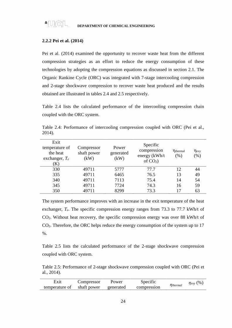
2.2.2 Pei et al. (2014)
Pei et al. (2014) examined the opportunity to recover waste heat from the different
compression strategies as an effort to reduce the energy consumption of these
technologies by adopting the compression equations as discussed in section 2.1. The
Organic Rankine Cycle (ORC) was integrated with 7-stage intercooling compression
and 2-stage shockwave compression to recover waste heat produced and the results
obtained are illustrated in tables 2.4 and 2.5 respectively.
Table 2.4 lists the calculated performance of the intercooling compression chain
coupled with the ORC system.
Table 2.4: Performance of intercooling compression coupled with ORC (Pei et al.,
2014).
Exit
temperature of
the heat
exchanger, Te
(K)
Compressor
shaft power
(kW)
Power
generated
(kW)
Specific
compression
energy (kWh/t
of CO2)
ηthermal
(%)
ηexy
(%)
330 49711 5777 77.7 12 44
335 49711 6465 76.5 13 49
340 49711 7113 75.4 14 54
345 49711 7724 74.3 16 59
350 49711 8299 73.3 17 63
The system performance improves with an increase in the exit temperature of the heat
exchanger, Te. The specific compression energy ranges from 73.3 to 77.7 kWh/t of
CO2. Without heat recovery, the specific compression energy was over 88 kWh/t of
CO2. Therefore, the ORC helps reduce the energy consumption of the system up to 17
%.
Table 2.5 lists the calculated performance of the 2-stage shockwave compression
coupled with ORC system.
Table 2.5: Performance of 2-stage shockwave compression coupled with ORC (Pei et
al., 2014).
Exit
temperature of
Compressor
shaft power
Power
generated
Specific
compression ηthermal
ηexy (%)

DEPARTMENT OF CHEMICAL ENGINEERING
25
the heat
exchanger , Te
(K)
(kW) (kW) energy (kWh/t
of CO2)
(%)
428 56891 16303 71.8 17 70
438 56891 16822 70.9 18 72
448 56891 17278 70.1 18 74
458 56891 17672 69.4 19 76
468 56891 18007 68.8 19 77
The specific compression energy is between 68.8 and 71.8 kWh/t of CO2, which is
lower than that in the case of intercooling compression (table 2.4). It is worth
mentioning that, without ORC coupling, the specific compression energy requirement
is 100.7 kWh/t of CO2, higher than for intercooling compression. Coupling the ORC
system resulted in compression savings of over 30 %, making shockwave
compression more advantageous than the intercooling option. Thanks to the higher
temperature of the pressurised CO2, the shockwave with ORC compression chain is
able to capture more waste heat and offset the compressor shaft power requirement,
rendering the shockwave compression more energy efficient than the intercooling
option. In other words, the waste heat provided by the shockwave compression has a
higher quality than that provided by the intercooling compression.
However, this reported study only focused on the 7-stage intercooling compression
and 2-stage shockwave compression, the other approaches or strategies such as
conventional in-line and multistage compression integrated with pumping also should
be considered in recovering waste heat as an effort in reducing the energy
consumption of the compression system.
2.2.3 Romeo et al. (2009)
Romeo et al. (2009) analysed and optimised the design of a CO2 intercooling
compression system by taking advantage of the low temperature heat duty in the low
pressure heaters of a steam cycle. In order to minimise the incremental Cost of
Electricity (COE) associated with CO2 compression, the introduction of a two stage
intercooling layout in 4-stage of compression is proposed. In the first stage, the
extracted heat could be used in the low-pressure part of the steam cycle for water pre-

DEPARTMENT OF CHEMICAL ENGINEERING
26
heating, while in the second stage, the extracted heat is dissipated in the cooling tower
after reduction of CO2 temperature and at the same time reduces the power
requirements of the compressor.
Based on their results, the authors concluded that the integration of CO2 intercooling
waste energy into the steam cycle reduces ca. 23 % of the incremental COE
associated with compression (approximately 0.8 €/MWh). In the meantime, a drop of
ca. 9 % of the compression cost from 25.1 M€ to 22.8 M€ can be observed when 80
% of the compressor efficiency is increased to 90 %. However, reducing the number
of stages from four to three with 80 % of efficiency increases ca. 0.19 €/MWh of the
COE. This proposed integration scheme can be used to reduce the energy and
efficiency penalty of CO2 capture processes thereby reducing the CO2 capture cost.
2.2.4 Moore et al. (2011)
Moore et al. (2011) presented a study on the development of novel compression and
pumping processes for CCS applications. An internally-cooled compressor diaphragm
was developed to remove the compressor heat using an optimal designed cooling
jacket based on a state of the art aerodynamic flow path without introducing an
additional pressure drop. An existing centrifugal compressor installed in a closed loop
test facility was retrofitted with the new cooled diaphragm concept.
From the validation results utilizing 3D CFD and experimental data, an optimal
design was achieved that provided good heat transfer while adding no additional
pressure drop. Various tests conducted demonstrated the effectiveness of the design.
However, the above studies (Romeo et al., (2009) and Moore et al., (2011)) did not
explore the energy saving potential in CO2 compression and liquefaction process.
Considering that there is abundant heat resource in coal-fired power plants, especially
the exhaust heat with low temperature. The exhaust heat with lower level can be
utilised to decrease the energy consumption in the process of CO2 compression and
liquefaction, which will be helpful to reduce the thermal efficiency penalty when CCS
is applied in power plants.

DEPARTMENT OF CHEMICAL ENGINEERING
27
2.2.5 Duan et al. (2013)
Duan et al. (2013) analysed and compared the energy consumptions of conventional
systems and a new process for CO2 compression and liquefaction. The conventional
method involves a four-stage gas compression while the new method employs three-
stage gas compression and one stage pump pressurisation. The refrigeration process
driven by the lower level heat from the coal-fired power plant is integrated in the new
compression and liquefaction system. The cooling needed to liquefy the CO2 is
provided by an ammonia absorption refrigerator driven by exhaust heat.
Eight different cases have been investigated to study the effects of the refrigeration
temperature on the total energy consumption of CO2 compression and liquefaction.
The corresponding performance data for each system is presented in table 2.6. The
first case presents the conventional multistage compression with 30 oC water cooling
(C-C) and the remaining six cases are the single refrigeration compression with
different refrigeration temperature (R-C1 to R-C6) while, the last case employs a
double-effect refrigeration compression with two evaporation temperatures (DR-C).
As shown in table 2.6, the total energy consumption, WCO2 using conventional
methods to compress and liquefy CO2 is huge, reaching about 358.84 kJ/kg CO2.

DEPARTMENT OF CHEMICAL ENGINEERING
28
Table 2.6: Performance data of different CO2 compression and liquefaction processes (Duan et al., 2013).
Parameter C-C R-C1 R-C2 R-C3 R-C4 R-C5 R-C6 DR-C
Refrigeration temperature, tc (oC) 30 -15 -20 -25 -30 -35 -40 -15, -30
Initial pressure from capture, Pinitial (MPa) 0.1 0.1 0.1 0.1 0.1 0.1 0.1 0.1
Pressure at the inlet compressor, Pl (MPa) 7.2127 2.2908 1.9696 1.6827 1.4278 1.2024 1.0045 1.4278
Final pressure for pipeline transport, Pfinal (MPa) 8.1 8.1 8.1 8.1 8.1 8.1 8.1 8.1
Final temperature of liquid, tl (oC) 30 25 25 25 25 25 25 25
CR 3 3.85 2.73 2.57 2.43 2.31 2.16 2.43
Compression work, Wc (kJ/kg CO2) 357.56 222.75 208.89 190.69 175.33 160.81 143.95 175.33
Work consumption of liquid CO2 pump, W3
(kJ/kg CO2)
- 7.61 7.79 8.07 8.23 8.32 8.43 8.23
Cooling capacity to cool down per kg of CO2,
Qo (kJ/kg CO2)
- 347.7 363.4 379.2 385.2 374.4 361.8 385.2
Total heat absorbed by the circulating cooling
water to cool down per kg of CO2, QW
(kJ/kg CO2)
495.3 1040.6 1125.3 1221.8 1300.1 1336.7 1378.1 1107.8
Pump work for the circulating cooling water,
WW (kJ/kg CO2)
1.28 2.70 2.92 3.17 3.37 3.47 3.57 2.87
COP - 0.502 0.477 0.450 0.421 0.389 0.356 0.533
Thermal energy of hot fluid consumed by NH4,
QCO2 (kJ/kg CO2)
- 692.8 761.9 842.6 914.9 962.4 1016.3 722.7
Temperature of hot fluid, te (oC) - 137.8 145 151 159 167.5 175.5 159.0
Power influence coefficient, X - 0.0787 0.0838 0.0888 0.0939 0.0992 0.1046 0.0939
The converted work of the hot fluid, WCV (kJ/kg
CO2)
- 54.53 63.85 74.83 85.91 95.47 106.30 67.86
Total power consumption for compression and
liquefaction, WCO2 (kJ/kg CO2)
358.84 287.58 283.44 276.75 272.84 268.07 262.25 254.29

DEPARTMENT OF CHEMICAL ENGINEERING
29
The compressor work reaches 357.56 kJ/kg CO2, accounting for the major portion of
total energy consumption. When the new method is applied, the total energy
consumption of CO2 compression and liquefaction decreases with the decrease in the
refrigeration temperature, tc. The total energy consumption reduces by ca. 27 % for
the case of R-C6 as compared to the conventional method, C-C. For case DR-C with a
double-effect refrigeration compression, the total energy consumption is reduced up
to 254.29 kJ/kg CO2, with ca. 29 % decrease of energy consumption.
The advantage of lower energy consumption is reduced as the converted work of
extracted steam, WCV increases with the decrease in the refrigeration temperature.
Figure 2.5 shows the comparison of gas compression work and total work
consumption with and without recovering the cold energy of liquefied CO2 for CO2
compression and liquefaction in different cases.
Figure 2.5: Compression work and total work consumption for different CO2
compression scenarios (Duan et al., 2013).
Although the compression work, WCO2 decreases as the refrigeration temperature
drops, the total work consumption without cold energy recovery of liquid CO2 does

DEPARTMENT OF CHEMICAL ENGINEERING
30
not decrease continuously. This is because the converted work of the extracted steam
accounts for an increasing proportion of the total work consumption as the cooling
temperature decreases. The increased converted work neutralises the decreased
compression work, and in the refrigeration temperature range from -15 oC to -40 oC,
the total power consumption without recovering cold energy of liquid CO2 decreases
slightly at first and increases soon afterwards. Thus, in some cases for the fixed
refrigerator performance, the refrigeration temperature should not be set too low.
Evidently, there exists an optimal refrigeration temperature for minimising the total
power consumption. In the case of DR-C process, CO2 was cooled by double-effect
refrigerator in the refrigeration process that provides the different levels of cold
energy. Applying this process reduces the exergy loss of heat transfer and increases
the cooling efficiency of the refrigerator. As can be seen from figure 2.5, the DR-C
process with -15 oC and -30 oC evaporation temperatures has the lowest total power
consumption out of the eight cases. Table 2.7 shows the comparison results from the
Pulverised Coal (PC) plant with and without CO2 capture process.
Table 2.7: The comparison results of different CO2 compression methods (Duan et al.,
2013).
Parameter PC without
CO2 capture
PC+CCS CO2
compression with
the conventional
method
PC+CCS CO2
compression
with new method
Gross power plant (MW) 604.3 533.16 527.78
Power plant inner loss (MW) 30.22 30.22 30.22
CO2 capture power (MW) - 21.28 21.28
CO2 compression power
(MW)
- 28.62 14.55
Plant electrical power
consumption (MW)
30.22 80.12 66.05
Plant net output power (MW) 574.09 453.04 461.73
Power plant net thermal
efficiency (%)
40.28 31.79 32.40
Efficiency loss (%) - 8.49 7.88
CO2 recovery ratio (%) - 85 85
CO2 emission (generator
output) (g/kWh)
566.3 94.9 95.87
Reduced CO2 emission
(generator output) (g/kWh)
- 535.3 540.76

DEPARTMENT OF CHEMICAL ENGINEERING
31
The CO2 compression power requirement in case of integrating the power plant with
the CCS and a conventional compression and liquefaction method was 28.62 MW,
compared to 14.55 MW in case of the power plant with the CCS and the refrigerating
compression combined with exhausted heat utilisation (new method).
Advantageously, the drop in compression power also results in an increase in the net
power output of the plant. According to the data in table 2.7, using the conventional
method to compress and liquefy CO2, results in an efficiency loss of 8.49 % as
compared to PC plant without CO2 capture when the net thermal efficiency of the
power plant drops from 40.28 to 31.79 %. On the other hand, when the new
compression method is employed, the efficiency loss decreases to 7.88 %, and the net
thermal efficiency of the power plant will be 32.40 %, corresponding to a marginal
increase of 0.61 %.
According to Duan et al. (2013), a large amount of low quality heat is demanded in
the refrigerating compression combined with exhausted heat utilisation process which
occupies a big proportion of the total power consumption if the heat is converted into
work. However, this process is especially suitable for coal-fired power plants which
have a large amount of lower level heat and need to compress and liquefy CO2 in a
large scale.
In this reported study, the new process for CO2 compression and liquefaction
employing complex refrigeration system powered by exhaust heat will need plenty of
mechanical work to produce the low temperature. The liquefaction and pumping
equipment also will entail additional capital expenses compared to conventional
compression system.
2.2.6 Modekurti et al. (2017)
Modekurti et al. (2017) investigated the performance of both an inline and integral
gear multistage compressor to compress the CO2 stream in the gas phase to
supercritical conditions by considering the variable mass flow rate during a flexible
operation in the power plant. The compression systems during steady state and

DEPARTMENT OF CHEMICAL ENGINEERING
32
transient conditions modelled accounting for inter-stage coolers, flash vessel, glycol
tower and the CO2 inventory from a post-combustion CO2 capture process.
According to the results presented by Modekurti et al. (2017), the inline compressor
system consumes ca. 29700 kW, which is 19 % more than that for the 8-stage integral
gear compressor system for compressing the CO2 stream from 1.15 to 152.8 bar as
shown in table 2.8. This difference compares well with the work of Wacker and Kisor
(2012), where the authors have reported 18 % more power consumption for
compressing CO2 from 1 bara to 150 bara in an inline compressor with 2 sections, a
total of 15 stages, and 3 intercoolers in comparison to an integral gear compressor
with 8 stages and 6 intercoolers. However, a high amount of recoverable heat
produced from the coolers in the inline compressor that can be used elsewhere, such
as providing heat to the reboiler of the CO2 capture system or for generating steam.
Table 2.8: Compressor comparison summary (Modekurti et al., 2017).
Integral gear Inline
Total power (kW) 24970 29700
Average polytropic efficiency (%) 84.7 84.0
Total cooling (kWth) 44900 48000
TEG reboiler duty (kWth reboiler at 121 oC) 790 1340
Recoverable heat (kWth above 121 oC) 900 23550
CO2 recycle from the TEG stripper (%) 2.25 3.0
Concentration of CO2 in the feed to the compression system can vary due to
operational changes in the CO2 capture system. According to Modekurti et al. (2017),
all the compressor stages will approach the surge condition when the mass flow rate
reduces to 45 % reduction.
However, based on the results presented in table 2.8, the total power reported for both
integral gear with 8 stages and 6 intercoolers and inline compressor with 15 stages
and 3 intercoolers are approximately 50 % below than the reported values from
Witkowski and Majkut (2012) and Witkowski et al., (2013).
While the above studies (Witkowski and Majkut (2012), Witkowski et al., (2013), Pei
et al., (2014), Romeo et al., (2009), Moore et al., (2011) and Modekurti et al., (2017))
have primarily focused on the development of suitable compression strategies for
DEPARTMENT OF CHEMICAL ENGINEERING
33
high-purity CO2, it has also been recognised that CO2 streams in CCS inevitably carry
some amount of impurities, whose nature and concentrations depend on the emission
source and capture technology applied. These impurities are expected to reduce the
effective storage capacity of the reservoir and also affect the physical properties and
vapour-liquid phase equilibrium of the CO2 stream, directly impacting the design of
compression equipment and the CO2 pipeline transport.
2.2.7 Aspelund and Jordal (2007)
Aspelund and Jordal (2007) investigated and compared three different CO2 transport
chains using both pipeline and ship. The first chain (P1) consists of compression to 60
bar, liquefaction of CO2 stream using sea water at 10 oC and pumping to 150 bar
while the second chain (P2) involves direct compression to 150 bar. In both P1 and
P2, the gas is compressed in centrifugal compressors in four stages. In case of the ship
transport process (S1), the gas stream is conditioned to ship and reservoir
specifications before liquefaction at ca. 6-7 bar at -52 oC. The liquid stream is then
sent to an intermediate storage before being pumped to a ship-based transport, which
transports the CO2 stream to the sequestration site.
From the reported results shown in figure 2.6, process chain P1 shows approximately
10 % higher energy efficiency compared to P2 and S1. At atmospheric pressure, the
energy requirement for P1 and P2 or S1 is approximately 95 and 105 kWh/tonne CO2,
respectively. Thus, P1 is the preferred solution for process plants with access to sea
water with a relatively low temperature. However, P2 will have lower investment
costs and is favourable for higher seawater temperatures.

DEPARTMENT OF CHEMICAL ENGINEERING
34
Figure 2.6: Variation of energy requirement for P1, P2 and S1 as a function of inlet
pressure (Aspelund and Jordal, 2007).
The effect of volatiles by adding nitrogen to the feed is shown in figure 2.7.
Figure 2.7: Variation of energy requirement for P1, P2 and S1 as a function of inert
gas content (Aspelund and Jordal, 2007).
As expected the power requirements for the process with direct compression (P2)
increases linearly with the increases of nitrogen content in the feed by approximately
2 kWh/mole nitrogen. In the case of P1 and S1 which involve the liquefaction of CO2
and the removal of the volatiles in an inert column, a linear increase in power
requirements of ca. 6 kWh/mole nitrogen can be observed in figure 2.7. According to
the authors, the presence of large amount of volatiles in the captured CO2 stream will
DEPARTMENT OF CHEMICAL ENGINEERING
35
increase the bubble point pressure of the mixture as well as increase the column
condenser and re-boiler duty.
2.2.8 de Visser et al. (2008)
de Visser et al. (2008) investigated the range of allowable concentrations of impurities
in the pre-combustion stream for safe transportation in pipelines. The issues addressed
in the authors work are safety and toxicity limits, hydrate formation, corrosion, free
water formation as well as compression work. Compression work calculations for a
representative CCS stream from 14.5 to 150 bar have been conducted including small
percentages of non-condensable gases, using two alternative compression processes
which are condensation by cooling and pumping and multi-stage compression. The
results show that the increase in compression work depends linearly on the
concentration of the gaseous impurity and it is approximately 2.5, 3.5 and 4.5 % for a
concentration of 1 % of O2, N2 and H2, respectively. In addition, the results also show
that both the total compression work and the impact of other components vary with
the selection of compression process. All non-condensable gases require additional
compression work, but the effect of hydrogen is the strongest.
2.2.9 Goos et al. (2011)
Goos et al. (2011) determined the specific energy consumption of the compression
process for the different CO2-N2 gas mixtures. The captured CO2 stream at 50 oC and
1 bar with the flow rate of 1000 kmol/h is compressed using an 8-stage compressor
compressed to the final pressure of 110 bar. Their simulations are performed
employing PRO/II software (McMullen, 2016) and the results are presented in table
2.9.
Table 2.9: Comparison of the specific compression power for different CO2 gas
mixtures compressed to 110 bar (Goos et al., 2011).
Gas
mixture Composition
Specific energy
(kWh/t CO2)
Density (kg/m3)
(Kunz et al., 2007)
1 100 mole % CO2 86 792
2 95 mole % CO2, 5 mole % N2 87 681
3 90 mole % CO2, 10 mole % N2 88 536

DEPARTMENT OF CHEMICAL ENGINEERING
36
4 80 mole % CO2, 20 mole % N2 89 343
From the results presented in table 2.9, it can be seen that by increasing the impurity
in the CO2 stream, the specific compression power requirement to drive the
compressor to reach the end condition will be increased. In particular, the
compression power is inversely proportional to the fluid density which progressively
decreases with the existence of impurities.
2.2.10 Chaczykowski and Osiadacz (2012)
Chaczykowski and Osiadacz (2012) carried out simulations to compare the
compression power for different CO2 mixture compositions corresponding to different
capture technologies under transient flow conditions. The variable CO2 production
rates are simulated, assuming the mass flow rate in the capture plant varies linearly at
a rate of 0.25 kg/min between the values of 40 and 100 kg/s. The compressor suction
pressure of 0.2 MPa and suction temperature of 40 oC is employed and results are
illustrated in figure 2.8.
Figure 2.8: Variation of compressor station power (Chaczykowski and Osiadacz,
2012).
According to the data in figure 2.8, the compression power for the 24 hours
simulation period in the case of oxy-fuel stream is 24.5 MW, compared to 21.83 MW
in the case of pure CO2 stream. For pre-combustion and post-combustion streams, the
figures are 22.54 and 22 MW respectively. Therefore, the total energy demand for the
transportation of oxy-fuel, pre-combustion and post-combustion mixtures in the

DEPARTMENT OF CHEMICAL ENGINEERING
37
simulation period is respectively, 12.2, 3.2 and 0.78 % higher than that of the pure
CO2 stream. Based on the figure 2.8, it may be reasonably concluded that in the case
of oxy-fuel and pre-combustion technologies, the compressors and after-cooler
facilities will incur higher operational costs due to the higher fuel and electric power
consumption.
Based on the above studies (Aspelund and Jordal (2007), de Visser et al., (2008),
Goos et al., (2011) and Chaczykowski and Osiadacz (2012)), in order to minimise the
compression costs associated with the presence of impurities in the CO2 stream,
optimising the CO2 separation and purification processes should be investigated. In
the case of relatively small CO2 emission sources, compression and transportation of
low-grade CO2 carrying more than 5 % of impurities, may be required prior to its
further purification. However, to date, the compression requirements for industrial
low-grade CO2 streams have not been systematically assessed.
2.3 Concluding remarks
In this chapter the basic thermodynamic and energy balance relations for calculating
the power requirement of multistage compression and cooling duty were presented.
These presented equations coupled with a Cubic Equation of State representing the
foundation of the multistage compression model. The thermodynamic relations for
predicting the pertinent fluid properties such as the fluid enthalpy, entropy and
discharge temperature were presented.
In chapter 3, the details for the calculation of compression power consumption and
cooling duty are presented. Particular attention is paid to the Peng-Robinson Equation
of State as a solution to determine the thermodynamic properties given its popularity
due to its accuracy and robustness.
It is also clear that most of the above review employed the conventional CO2
compression strategy which is responsible for a large portion of the enormous capital
and operating cost penalties as well as sizable parasitic energy consumer. Thus, it is
incompatible with the original intention of energy saving and emission reduction. Any
approach or strategy resulting in a reduction in the CO2 compression workload
DEPARTMENT OF CHEMICAL ENGINEERING
38
directly contributes to an improvement of net plant efficiency. It is the purpose of this
thesis to investigate different compression strategies and identify the optimum number
of stage of compression system to minimise the associated cost and energy penalties.
While the above reported studies also quantified the power requirements for industrial
compression of CO2, their practical application is, however, limited due to the
underlying assumption of negligibly amounts of impurities in the CO2 stream. In
practice, the CO2 streams in CCS will contain some impurities with range and level,
mostly depending on the capture technology. The impact of a varying CO2 stream
concentration on the compression power requirement is not fully understood.
In chapter 3, the selection of an appropriate compression strategy for realistic CO2
streams and associated compression work penalty costs is investigated.
2.4 Modelling of transient fluid flow in pipelines
The development of a transient flow model is based on the application of the
governing equations of fluid dynamics. These equations are derived from the
fundamental physical principles by assuming mass, momentum and energy are
conserved. However, with respect to the pipeline flow, their precise formulation
depends on a number of considerations such as interface topology, multi-component
exchanges, dissipative fluid/wall interactions, pipeline elasticity and rigidity as well as
pipeline elevation (Menon, 2005, Bratland, 2009).
In essence, interface topology accounts for various flow regimes. These, for example,
may include fully dispersed two-phase, stratified, annular or churn flows. Multi-
component exchanges on the other hand deal with equilibrium as opposed to non-
equilibrium effects. Dissipative fluid/wall interactions represent the effects resulting
from heat transfer and friction. Pipeline elasticity and rigidity refer to the degree of
compliance and as to whether or not the pipeline is rigidly clamped. Pipeline elevation
on the other hand accounts for unevenness in terrain and considers the effect of
gravity on fluid flow in the pipeline. The degree of complexity of any mathematical
model developed is closely related to its ability to adequately incorporate all the
above mentioned effects in its formulation.

DEPARTMENT OF CHEMICAL ENGINEERING
39
Consequently, a detailed model should comprise of the equations of mass, momentum
and energy conservation for turbulent single/multi-phase flow, and should account for
some, if not all, of the effects mentioned earlier. For these, the Navier-Stokes
equations represent the most complete formulation that describes any fluid flow
situation (Bratland, 2009). These equations allow for the variation of fluid property in
four dimensions, i.e. the three dimensions of space, x, y, and z, and also time, t.
However, the solution of the full system of these equations and the numerical
discretisation necessary to accomplish this for a whole range of fluid flows is
extremely difficult and requires substantial computational resources. Nevertheless,
depending on the type of flow scenario that needs to be resolved, certain terms in the
equations will have a negligible effect on the final solution and can be safely ignored
without any serious loss of accuracy. At the same time, advantageously, these
simplifications generally lead to less computationally expensive models, but on the
other: the greater the simplification, the higher the likelihood of introducing
modelling inaccuracies. Nonetheless, the final form of the conservation equations,
derived through simplifying assumptions, may, in the more general classification, be
linear, quasi-linear or non-linear, parabolic or hyperbolic, and first- or second-order.
There has been much research activity in the field of theoretical modelling of fluid
flow transients. Various assumptions and simplifications have been made in order to
suit a particular method of solution or application. Suwan and Anderson (1992)
argued that alternative formulations, interpolations, friction force representation, or
time integration, which may be appropriate for parabolic problems, will all violate the
basic wave like characteristics of a hyperbolic problem. Most cases of unsteady
one-dimensional flow where disturbance propagation velocities do not vary
significantly are characterised by quasi-linear hyperbolic partial differential equations
for continuity and momentum. On the other hand, complex phenomena such as
stratified and intermittent stratified-bubble (slug) flows require a two-dimensional
transient analysis for a complete treatment of the problem.
Various analytical techniques have been used to reduce the number of equations
before employing the relevant numerical procedure. van Deen and Reintsema (1983)

DEPARTMENT OF CHEMICAL ENGINEERING
40
for example, introduced a technique which reduces the energy equation to a single
parameter-in-mass equation without the assumption of isothermal or isentropic flow.
In fluid flow problems the dependent variables i.e. pressure, P, density, , and
velocity, v are functions of the independent variables i.e. time, t and distance, x in the
case of one-dimensional flow. In any given flow situation, the determination by
experiment or theory of the fluid properties as a function of x and t is considered to be
the solution to the problem. There are two distinct fundamental ways of specifying the
flow field, namely the Lagrangian and Eulerian descriptions (Sidek, 2013).
In the Lagrangian approach, the fluid is considered to comprise a large number of
finite sized fluid particles which have mass, momentum, internal energy and other
properties. The mathematical equations are derived for each fluid particle. A major
drawback of this approach is restrictively time consuming when considering even a
very small volume of fluid. Even when a gas is being considered where there are few
molecules, a relatively larger time-step compared to the Eulerian approach must to be
employed due to the longer mean free path of the molecules resulted in lower
computational run times (Sidek, 2013).
The Eulerian approach considers how the flow properties change at a fluid element as
function of time and space. The information about the flow is obtained in terms of
what happens at fixed points in space as the fluid flows through those points (Sidek,
2013).
According to Richtmyer (1960), the Lagrangian approach is generally preferred for
some problems in a one space variable. For problems in two or more space variables
and time, the Lagrangian method encounters serious difficulties. In particular, the
accuracy usually decreases significantly as time goes on, due to distortions, unless a
new Lagrangian point-net is defined from time to time, which requires cumbersome
and usually rather inaccurate interpolations.
In fluid dynamics measurements, the Eulerian method is the most suitable. The
Eulerian formulation has almost exclusively been used in all recent studies even

DEPARTMENT OF CHEMICAL ENGINEERING
41
through in some cases according to the above discussion, the Lagrangian description
would seem more appropriate (Sidek, 2013).
In the deriving the conservation equations, both descriptions are used depending on
the circumstance, with the Euler concept being denoted by t
a
or
x
a
and the
Lagrange concept being denoted byDt
Da (Price, 2006). The relationship between the
two is given by,
x
av
t
a
Dt
Da
2.35
where a denotes pressure, density, velocity etc. of the fluid flows in the pipeline.
In the following section, the mathematical model used to simulate the transient flow
in a pipeline is derived. The equations will be derived from first principles and any
assumptions or simplifications will be accounted for.
2.4.1 Model assumptions
In this section, the following assumptions are employed in the development of the
numerical pipeline fluid flow model:
Steady state exists prior to the transient conditions. The fluid properties
obtained from a steady state calculation act as the initial conditions required
for the hyperbolic system.
The flow is predominantly one-dimensional, that is, the rate of change of flow
variables normal to the axial direction is negligible relative to those along the
axial direction.
When multiphase are present, the phases are assumed to be homogeneously
mixed and in thermodynamic equilibrium at all times during the transient flow
conditions.
Each pipeline is rigidly clamped and of uniform cross sectional area.
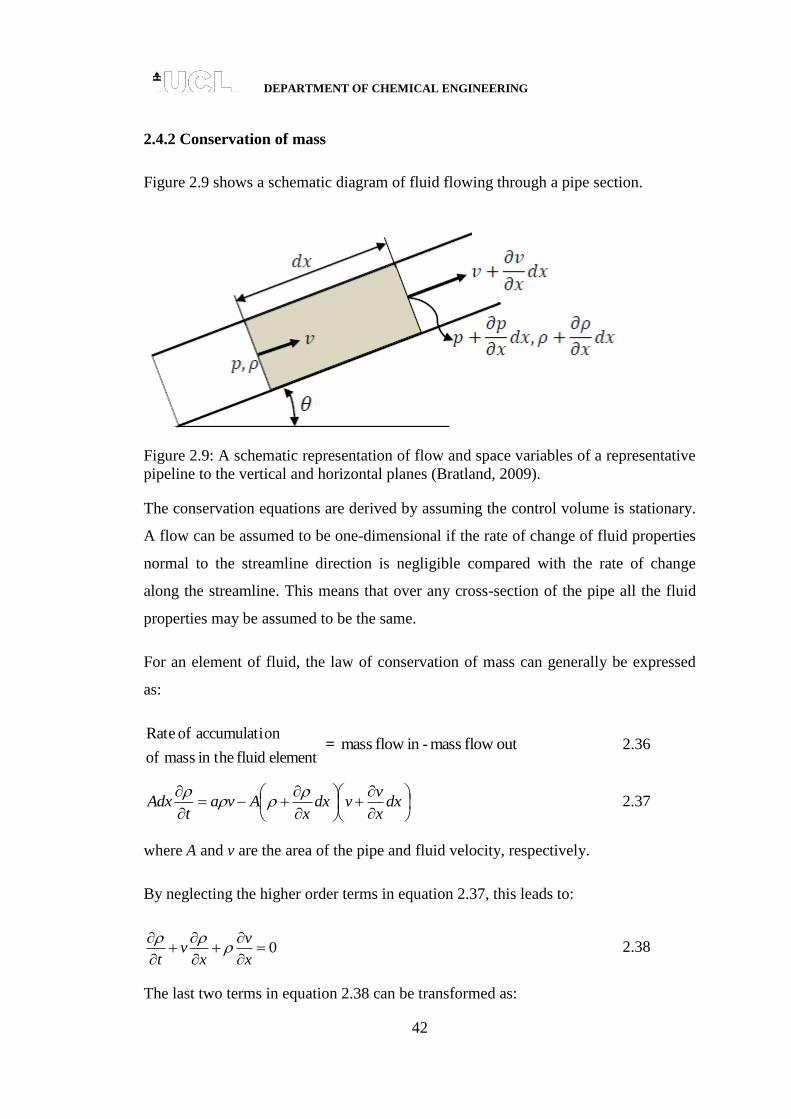
DEPARTMENT OF CHEMICAL ENGINEERING
42
2.4.2 Conservation of mass
Figure 2.9 shows a schematic diagram of fluid flowing through a pipe section.
Figure 2.9: A schematic representation of flow and space variables of a representative
pipeline to the vertical and horizontal planes (Bratland, 2009).
The conservation equations are derived by assuming the control volume is stationary.
A flow can be assumed to be one-dimensional if the rate of change of fluid properties
normal to the streamline direction is negligible compared with the rate of change
along the streamline. This means that over any cross-section of the pipe all the fluid
properties may be assumed to be the same.
For an element of fluid, the law of conservation of mass can generally be expressed
as:
element fluid in the mass of
onaccumulati of Rate = in flow mass - out flow mass 2.36
dx
x
vvdx
xAva
tAdx
2.37
where A and v are the area of the pipe and fluid velocity, respectively.
By neglecting the higher order terms in equation 2.37, this leads to:
0
x
v
xv
t
2.38
The last two terms in equation 2.38 can be transformed as:

DEPARTMENT OF CHEMICAL ENGINEERING
43
x
v
x
v
xv
2.39
In the case of one-dimensional flow, the mass conservation equation is represented as:
0
x
v
t
2.40
With the aid of suitable thermodynamic relations, the total derivative of density with
respect to time and space in equation 2.40 can be reformulated and expressed in terms
of fluid pressure and enthalpy/entropy. This reformulation enables the derivative
terms in the conservation equations to be expressed only in terms of fluid pressure,
enthalpy/entropy and velocity. The importance of this approach, especially with
respect to reduction in computational run time, is elaborated latter.
For any fluid, the fluid pressure can be expressed as a function of density, and
entropy, s i.e., P = f (, s). Thus, in partial differential form, this relationship can be
written as:
dss
Pd
PdP
s
2.41
where:
2aP
s
2.42
s
P 2.43
Hence by substituting equations 2.42 and 2.43 into equation 2.41, the substantial
derivative of pressure with time can be expressed as:
dt
ds
dt
da
dt
dP
2
2.44
By rearranging equation 2.44 and making the total derivative of density as the subject
gives:
DEPARTMENT OF CHEMICAL ENGINEERING
44
dt
ds
dt
dP
adt
d
2
1 2.45
For any fluid, the total derivative of enthalpy is given by Walas (1985):
dPTdsdh
1 2.46
Thus from equation 2.46, the total derivative for enthalpy with respect to time
becomes:
dt
dP
dt
dsT
dt
dh
1 2.47
Rearranging equation 2.47 gives:
dt
ds
dt
dP
dt
dh
T
11 2.48
Substituting equation 2.48 into equation 2.44 by replacing the total derivative of
entropy with time results in:
dt
dP
dt
dh
Tdt
da
dt
dP
12 2.49
By rearranging equation 2.49, an expression for the total derivative of density with
respect to time in terms of fluid pressure and enthalpy is obtained as:
dt
dh
TTdt
dP
adt
d
1
12
2.50
Substituting equations 2.45 or 2.50 into equation 2.40 gives:
02
x
va
dt
ds
dt
dP 2.51
022
x
vTa
dt
dh
dt
dPT 2.52

DEPARTMENT OF CHEMICAL ENGINEERING
45
Equations 2.51 and 2.52 represent the reformulated mass conservation equation for
one-dimensional flow in terms of pressure-entropy and pressure-enthalpy,
respectively.
2.4.3 Conservation of momentum
The momentum conservation equation is derived from the application of Newton’s
second law of motion. By applying this law to the control volume as shown in figure
2.9, gives (Bratland, 2009):
gravity friction force pressurenet on accelerati Mass 2.53
sin2
gdxAAvvd
dxfAdx
x
PPPA
dt
dvdxA w
2.54
where dt
dv, P, fw, v, g and θ are the acceleration, pressure, friction factor, velocity,
gravity and degree of the inclination of the pipe, respectively. Equation 2.54 can
reformulate to give:
sin2
gvvd
f
x
P
dt
dv w
2.55
where,
dt
dx
x
v
t
v
dt
dv
2.56
By inserting equation 2.56 into equation 2.55 gives:
sin2
gvvd
f
x
P
x
vv
t
v w
2.57
The left hand side of equation 2.57 describes the inertia part of Newton’s equation. It
has two terms, indicating that each fluid particle can accelerate both in time and
space.

DEPARTMENT OF CHEMICAL ENGINEERING
46
2.4.4 Conservation of energy
Heat flow can have a major impact on pipeline hydraulics, and accurate pipeline
modelling often require the underlying model to include thermal effects. This is
particularly true for compressible fluid flow, since the fluid’s temperature strongly
affects density. Energy conservation means that net energy coming in to the fluid has
to accumulate within it and can be presented as:
fluid theinsideenergy of
change of Rate=
fluid the
intoflux heat Net +
fluid on the
done work of Rate 2.58
The term on the left hand side (LHS) of equation 2.58 can be written as (Bratland,
2009):
sAdxEdt
dLHS 2.59
where ρAdx and Es are the control volume’s total mass and total energy per unit mass,
respectively. By assuming ρAdx is a constant, equation 2.59 gives:
dt
dEAdxLHS s 2.60
Equation 2.60 is reformulated to give:
x
Ev
t
EAdxLHS ss 2.61
From equation 2.61, it is given by:
x
Ev
x
vE
tE
t
E
x
vE
t
E sss
sss
2.62
The continuity equation 2.40 implies:
0
x
vE
tE ss
2.63
And therefore, equation 2.62 reduces to:
DEPARTMENT OF CHEMICAL ENGINEERING
47
x
Ev
t
E
x
vE
t
E ssss
2.64
By inserting equation 2.64 into equation 2.61,
x
vE
t
EAdxLHS ss
2.65
The specific energy Es in the control volume has three parts:
gzv
uEs 2
2
2.66
where u, 2
2vand gz are the fluid’s specific internal energy, the kinetic energy and the
potential energy due to the elevation, z from a reference level, respectively.
On the right hand side (RHS) of the equation 2.58, the only heat coming from the
surroundings into the pipe is the convection going through the pipe wall. The heat per
unit volume of pipe, q is the net heat flux into the element.
The last term in equation 2.58, rate of work done on the element is the net rate of
work done by pressure in the axial direction, x. Since forces in the positive x-direction
do positive work, a growing pv means negative work is done, and so:
dxA
x
PvqAdxRHS
2.67
Combining equations 2.65, 2.66 and 2.67 gives:
qP
gzv
uvx
gzv
ut
22
22
2.68
Introducing the enthalpy, h, which by definition is:
puh 2.69
Equation 2.68 is transformed into:

DEPARTMENT OF CHEMICAL ENGINEERING
48
qgzv
hvx
gzv
ut
22
22
2.70
Expanding the brackets in equation 2.70 gives:
q
x
zvg
x
vgz
x
vv
x
vv
x
vh
dx
hv
tgz
t
zg
t
uu
t
uu
tu
t
u
22
22 2.71
where,
sin
x
z 2.72
Since the pipeline inclination is time invariant, hence:
0
t
z 2.73
Substituting equations 2.72 and 2.73 into equation 2.70 and rearranging gives:
sin22
22
gvqv
hvx
vu
t
2.74
Substituting equations 2.40 and 2.55 into equation 2.74 and rearranging gives:
D
vfq
dt
dP
dt
dh w
2
3 2.75
However, the energy equation can be expressed alternatively in terms of the fluid
entropy. When the equation 2.48 is multiplied by ρT and becomes:
dt
dsT
dt
dP
dt
dh 2.76
Substituting equations 2.76 into equation 2.75 and rearranging gives:
D
vfq
dt
dsT w
2
3 2.77

DEPARTMENT OF CHEMICAL ENGINEERING
49
Equation 2.77 is the energy conservation equation in terms of fluid entropy for one-
dimensional flow.
From the above, it may be observed that the final expression of the conservation
equations is in terms of ‘direct’ (i.e. velocity, pressure and entropy/enthalpy) rather
than ‘conservative’ variables (i.e. density, momentum, and total energy). Expressing
the conservation equations in the direct variable form is essential in order to compute
correctly the propagation speed and the intensity of discontinuities such as shock
waves and contact surfaces that can occur in inviscid flows (LeVeque, 2002).
2.4.5 Thermodynamic analysis
The following subsection presents the main equations and correlations employed for
determining the two-phase mixture density, thermodynamic function and the heat
transferred to the fluid in the pipeline system.
2.4.5.1 Equation of State (EOS)
For the case of compressible flow, a relation in addition to the conservation equations
for mass, momentum and energy needs to be provided to ensure that the problem is
well-posed, mathematically. This relation is the Equation of State (EOS) which relates
thermodynamic properties and is divided into two categories. These are the
specialised EOSs, like GERG EOS (GERG, 2004) and general EOSs, like Van der
Waals cubic EOS. The performances of different EOS vary for different properties,
components and conditions of the fluid (Li et al., 2011).
Many types of EOS have been reviewed concerning thermodynamic property
calculations of CO2 mixtures, but the evaluation results of the EOS performance have
not pointed to one particular EOS. The general cubic EOS still show advantages over
more complicated or specialised EOS in the calculation of Vapour Liquid Equilibria
(VLE), while for volume calculations they cannot compete with equations such as
Lee-Kesler (LK) and Statistical Associating Fluid Theory (SAFT) (Li et al., 2011).
Based on the study by Li et al. (2011), seven general cubic EOSs were evaluated
using many of the experimental data concerning the VLE and the density of CO2

DEPARTMENT OF CHEMICAL ENGINEERING
50
mixtures including CH4, N2, O2, H2S, SO2 and Ar. The EOSs evaluated were Peng-
Robinson (PR) (Peng and Robinson, 1976), Redlich-Kwong (RK) (Redlich and
Kwong, 1949), Soave-Redlich-Kwong (SRK) (Soave, 1972), Patel-Teja (PT) (Patel
and Teja, 1982), 3P1T (Yu et al., 1987), PR-Peneloux (Paul et al., 1989), SRK-
Peneloux (Peneloux and Rauzy, 1982), and the improved SRK (Ji and Lempe, 1997).
The binary interaction parameters, kij, were calibrated with respect to the VLE data
available. In general, with calibrated kij, the cubic EOS gave an Absolute Average
Deviation (AAD) within 5 % for VLE calculations, and 6 % for calculations of the
density, except for the CO2/SO2 mixture. Vrabec et al. (2009) proposed to use the PR
EOS combined with a model based on Henry’s law constants for the ternary mixture
CO2/N2/O2 at low temperatures (218-251 K). Their results show that the PR EOS
describes both binary and ternary experimental data well, except at high pressures
close to the critical region. Wilhelmsen et al. (2012) reported that the SRK and PR
give are reasonable prediction for the density and the specific heat capacity in the
vapour region whereas deviations above 10 % should be expected in the liquid and
supercritical regions for the density of pure CO2.
Furthermore, it is no doubt that more accurate models such as specialised EOSs are
always preferable. More parameters will have to be included to improve the accuracy
of this EOS. The GERG EOS for example is principally different from the other EOS
because its formulation is based on a multi-fluid approximation, which is explicit in
the reduced Helmholtz energy depending on the density, the temperature and the
composition. The accuracy of the GERG EOS claims to be very high and the normal
range of validity covers temperatures between 90 K and 450 K and pressures less than
35 MPa. This covers a large part of the T/P range for CCS applications, except
regions with large temperatures or large pressures. The reported uncertainty of the
EOS regarding gas phase density and the speed of sound is less than 0.1 % from 250
K/270 K to 450 K and pressures up to 35 MPa. In the liquid phase of many binary and
multicomponent mixtures, the uncertainty of the equation regarding the density is less
than 0.1-0.5 %.

DEPARTMENT OF CHEMICAL ENGINEERING
51
Mazzoccoli et al. (2012) reported the study on predicting densities of CO2 and CO2-
mixtures containing N2 and CH4 using different EOS. Based on the authors’ study, the
GERG-2008 model showed the lowest deviations, however they were not negligible,
in particular in the phase equilibrium. Wilhelmsen et al. (2012) concluded that
GERG-2004 was the most accurate EOS for all the investigated mixtures (CO2-CH4,
CO2-N2, CO2-O2, N2-O2 and CO2-N2-O2) except those containing CO2-O2 in the two-
phase area, where it displayed an AAD of ~20 %. However, the runtime speed of the
GERG-2004 showed the most time demanding as compared to others EOS.
Given that the specialised EOS is a multi-parameter equation, it is prohibitively
computationally inefficient due to its complicated structures and hence impractical to
implement correctly for numerical simulations. The complex structure of the
specialised EOS makes the calculation of properties computationally demanding.
Because of this situation, general cubic EOS is usually preferred due to the simplest
structure and capable of giving reasonable results for the properties of pure CO2 and
CO2 mixtures.
As a result, the Peng-Robinson (PR) EOS (Peng and Robinson, 1976) is employed in
the present study. The details of this equation as previously derived can be found in
section 2.1.6.
2.4.5.2 Two-phase mixture density
In the case of liquid and gas mixture its density can be calculated using the PR EOS
pseudo-mixture density. This is given by:
xx lg
gl
1 2.78
where:
RTZ
PM
g
g
g 2.79

DEPARTMENT OF CHEMICAL ENGINEERING
52
RTZ
PM
l
ll 2.80
Here, x and Z are the fluid quality and compressibility factor, respectively. The
subscripts g and l represent the gas and the liquid phase of the fluid.
2.4.5.3 Single and two-phase determination of the thermodynamic function
The isochoric thermodynamic function, given by equations 2.51 and 2.52 for single-
phase fluids is given by Picard and Bishnoi (1987):
pC
Ta
s
P 2
2.81
where is the isobaric coefficient of volumetric expansion =pT
V
V
1. In the case of
two-phase flows, is calculated numerically in the following manner. Given that:
V
def
s
P
s
P
2.82
Using one of Maxwell’s relations (Walas, 1985):
sV
T
s
P
2.83
Since the specific volume,
1V :
2
1
d
dV 2.84
Equation 2.82 becomes:
s
T
s
P
2 2.85
Hence, from equation 2.82:

DEPARTMENT OF CHEMICAL ENGINEERING
53
ss
TT
22
2.86
For two-phase flows, φ can be evaluated numerically by using isentropic flash
calculation at a given temperature and pressure as proposed in Mahgerefteh et al.
(1997).
2.4.5.4 Fluid/wall heat transfer
In the case of flow in pipelines, the pipeline wall constitutes the immediate
surroundings of the fluid. However, except in the case of a perfectly insulated
pipeline, the overall external heat transferred to the fluid is influenced by wall and
ambient properties/conditions. Newton’s cooling law (Picard and Bishnoi, 1987,
Chen, 1979, Mahgerefteh et al., 1999) is commonly employed for determining the
heat transferred to a fluid flowing in a pipe. It is given by:
TTUD
q ambh
in
4
2.87
where Uh, Din and Tamb are the overall heat transfer coefficient, the pipeline inner
diameter and ambient temperature, respectively. In the present study, the Uh is taken
to be 5 W/m2K.
2.4.6 Hydrodynamic analysis
From the conservation equations derived in the sections 2.4.1-2.4.3, the
hydrodynamic parameters are calculated by employing the described equations in the
next subsection.
2.4.6.1 Calculation of Fanning friction factor
The Fanning friction factor, fw is required for calculating the contribution of frictional
force to the momentum equation (equation 2.57). It is a function of the flow
Reynolds’ number. The determination of this friction factor is depended on the
surface of the pipe wall and the flow mode of the fluid (Lipovka and Lipovka, 2014).

DEPARTMENT OF CHEMICAL ENGINEERING
54
Ouyang and Aziz (1996) conducted a study, over a wide range of flow
conditions8101Re2000( ; )1.010 6
inD
on the performance of 11 major
explicit correlations for predicting friction factor. The predictions of these correlations
were compared with the highly accurate Colebrook correlation (Colebrook, 1939).
Although the Colebrook correlation is accepted as the most accurate in terms of
predictions, it however has the disadvantage of expressing the friction factor in an
implicit form with the resultant equation requiring expensive iterations to solve
(Ouyang and Aziz, 1996). Many explicit approximations of the Colebrook equation
are available (Lipovka and Lipovka, 2014). These approximations vary in their degree
of accuracy, depending upon the complexity of their functional forms that generally
estimate friction factors with higher accuracy.
From the study conducted by Ouyang and Aziz (1996), the authors recommended the
use of the Chen (1979), Serghides (1984) and the Zigrang and Sylvester (1982)
correlations. These three were observed to show a maximum absolute deviation of
less than 1 % from the Colebrook correlation.
Based on the results reported by Ouyang and Aziz (1996), the Chen correlation is
employed in the present study for the calculation of the Fanning friction factor for
transition and turbulent flows in rough pipes as shown below:
8981.0
1098.1
Re
8506.5
8257.2
1lg
Re
0452.5
7065.3lg2
1
ininwDDf
2.88
where , Din and Re are the pipe roughness, internal diameter of the pipe and
Reynold’s number, respectively.
For turbulent flow in smooth pipelines, Rohsenow et al. (1998) recommend the
correlation proposed by Techo et al. (1965). The authors assert that the equation gives
predictions within 2 % of extensive experimental measurements. It is given by:
8215.3Reln964.1
Reln7372.1
1
wf 2.89

DEPARTMENT OF CHEMICAL ENGINEERING
55
In the laminar region, the evaluation of the Fanning friction factor is independent of
the pipe roughness. Thus in general, the Fanning friction factor for laminar fully
developed flow is given by Bratland (2009):
Re
16wf 2.90
2.4.6.2 Single and two-phase speed of sound determination
For single-phase real fluids, the speed of sound through the fluid can be expressed
analytically as (Picard and Bishnoi, 1987):
2ak
2.91
By definition, and k can be expressed respectively as (Walas, 1987):
P
V
C
C 2.92
T
Vk
P
2.93
where Cp and Cv are the specific heats at constant pressure and volume respectively,
and V is the specific volume of the fluid.
From equation 2.93, k can be obtained analytically by differentiating the PR EOS. For
two-phase flows, the analytical determination of and Cp becomes complex
(Mahgerefteh et al., 1999). Hence the speed of sound is evaluated numerically at a
given temperature and pressure as:
2
*, ,s
Pa
T P T P P
2.94
where the subscript, s and ΔP denote a constant entropy condition and infinitesimal
change in pressure (P = 1x10⁻⁶ atm), respectively. T* represents the corresponding
fluid temperature obtained by performing a (P-ΔP)/s flash.

DEPARTMENT OF CHEMICAL ENGINEERING
56
2.4.7 Numerical methods for the solution of transient fluid flow model
A variety of high-resolution numerical methods have been developed over the past
several decades that resolve discontinuities and rapidly changing flows sharply and
yet produce at least second-order accuracy in smooth flows. Understanding of the
different numerical methods available and appropriate implementation of a scheme
for the resolution of a particular problem requires not only a thorough grasp of the
physical nature of the flow being considered, but also a good foundation in the
mathematical theory of hyperbolic conservation laws.
The resulting system of equations in sections 2.4.1-2.4.3 was shown to be quasilinear
and hyperbolic in nature. As these equations contain terms that are unknown or non-
linear functions of their dependent and independent variables, they can only be solved
numerically (Mahgerefteh et al., 1999). Their complete solution also requires the
application of appropriate boundary conditions at the inlet and at the end of the
pipeline. These boundary conditions enable closure of the governing equations with
their solutions establishing the fluid dynamic and thermo-physical properties in time
and space along the pipeline. Three numerical techniques are commonly employed for
resolving hyperbolic partial differential equations which are Finite Difference
Methods (FDM), Finite Volume Methods (FVM) and Method of Characteristics
(MOC).
The FDM is a general mathematical technique that is widely applied to Partial
Differential Equations (PDEs). It involves discretising the spatial domain into a series
of nodes forming a grid. Finite approximations are then substituted for the derivatives
appearing in the PDEs taking values at the nodal points resulting in a system of
algebraic equations. Similarly, the FVM breaks the system up into a set of discrete
cells. The integral of the PDEs over each cell is approximated to produce a system of
algebraic relations. However, numerical diffusion associated with these methods
makes them unsuitable for modelling the transient flow following pipeline failure
(Mahgerefteh et al., 2009).

DEPARTMENT OF CHEMICAL ENGINEERING
57
The MOC is a mathematical technique that is particularly suited to the solution of
hyperbolic PDEs with two independent variables such as distance and time. The MOC
resolves the system of PDEs into a system of ordinary differential equations
(compatibility equations) through a particular co-ordinate change. These co-ordinates
represent curves (characteristic lines) in the space-time plane along which the
compatibility equations hold. The method is particularly suitable for systems
containing complex boundary conditions, as each boundary condition may be applied
individually to each characteristic curve moving into the computational domain
(Zucrow and Hoffman, 1975).
In this following section, the formulation and implementation of the MOC used to
solve the conservation equations governing single/two-phase homogeneous flow in
pipeline is presented.
2.4.7.1 Method of Characteristics (MOC)
The method of characteristics (MOC) is the natural numerical method for quasi-linear
hyperbolic systems with two independent variables (e.g. distance and time) (Thorley
and Tiley, 1987). It is based on the principle of the propagation of characteristic
waves and is therefore well suited to handling fast transient flow where each
disturbance is captured along the propagating Mach lines which are used in the
formulation of the final form of the finite difference equations (Zucrow and Hoffman,
1975).
In this method, the system of conservation equations as described in sections (2.4.1-
2.4.3) is assumed as quasilinear and hyperbolic. A PDE is said to be quasilinear if all
derivatives of the dependent function are linear, while their corresponding coefficients
may contain nonlinear terms. The conservation equations represented by equations
2.40, 2.57 and 2.74 are clearly linear in the partial derivative terms. Furthermore,
terms those are coefficients of the partial derivatives, such as the ρ or a are nonlinear
functions of P, s and v. The governing equations are therefore quasilinear in structure.
In the one-dimensional case, the governing equations 2.40, 2.57 and 2.74 can be
written in the general form as:

DEPARTMENT OF CHEMICAL ENGINEERING
58
Cx
UB
t
UA
2.95
where, A , U , B and C are given by:
v
s
P
U 2.96
0 T 0
0 0
0 1
A 2.97
0 0
0 1
- 2
Tv
v
avv
B
2.98
xh
x
vQ
gC
sin
0
2.99
A system of PDE as given by equation 2.95 is said to be hyperbolic if the eigenvalues
satisfying equation 2.100 given below are real and distinct (Prasad and Ravindran,
1985):
0 AB 2.100
Thus, for the conservation equations, the above equation may be expressed as:
0
0 0
0 1
- 2
TTv
v
avv
AB
2.101
Hence:
0)0(0 2 TTvavTTvvv 2.102
Simplifying equation 2.102 gives:

DEPARTMENT OF CHEMICAL ENGINEERING
59
02222 vTavTv 2.103
Factorising and dividing equation 2.103 by T2 gives:
022 avv 2.104
Solving equation 2.104 to obtain the roots of gives:
v1 2.105
av2 2.106
av3 2.107
It can be seen that the eigenvalues, i in equations 2.105-2.107 are real and distinct.
Thus, the system of conservation equations with partial derivatives in terms of P, s
and v are hyperbolic. This implies that the behaviour and properties of the physical
system described by these equations will be dominated by wave-like phenomena
(Prasad and Ravindran, 1985). Indeed the speed of propagation of these waves,
known as Mach lines, are given by the eigenvalues ( av ) and ( av ), which
correspond to the right running and left running characteristic (Mach) lines
respectively. The path line characteristic is given by 1. These characteristics can
handle any type of discontinuity in fluid flow such as a shock wave (Prasad and
Ravindran, 1985).
To adequately resolve a system of PDE in terms of three dependent variables (e.g. P, s
and v), three characteristic lines (i.e. the path line (C0), the positive (C+) and negative
(C-) Mach lines) need to be defined. These in essence govern the speed at which
expansion and compression waves propagate from the low and high-pressure ends of
the pipeline respectively (positive and negative Mach lines), while the path line
dictates the rate of flow through any given point along the pipeline. Their
corresponding compatibility equations may be solved by standard, single step finite-
difference methods for ordinary differential equations. Figure 2.10 is a schematic
representation of the characteristic lines at a grid point along the space, x and time t
independent coordinates.

DEPARTMENT OF CHEMICAL ENGINEERING
60
Figure 2.10: A schematic representation of Path line (C0) and Mach lines (C+, C-)
characteristics at a grid point along the time, t and space, x axis.
There are two main grid discretisation methods for the MOC. These are the
Characteristic Grid method (CG) which is also known as natural method of
characteristics (Wylie et al., 1971) or the Wave Tracing method (Chen, 1993), and the
Inverse Marching method which is also known as the Rectangular Grid method or the
Method of Specified Time Intervals (Flatt, 1986).
In the CG method, the position of the new solution point is not specified a priori, but
is determined from the intersection of left and right running characteristics with
origins located at known solution points or initial data. Hence a free floating grid is
developed in the x-t plane as shown in figure 2.11.
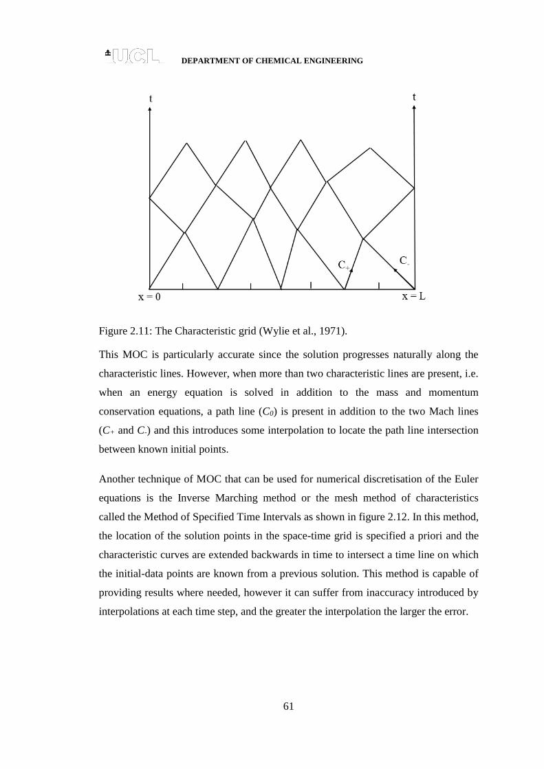
DEPARTMENT OF CHEMICAL ENGINEERING
61
Figure 2.11: The Characteristic grid (Wylie et al., 1971).
This MOC is particularly accurate since the solution progresses naturally along the
characteristic lines. However, when more than two characteristic lines are present, i.e.
when an energy equation is solved in addition to the mass and momentum
conservation equations, a path line (C0) is present in addition to the two Mach lines
(C+ and C-) and this introduces some interpolation to locate the path line intersection
between known initial points.
Another technique of MOC that can be used for numerical discretisation of the Euler
equations is the Inverse Marching method or the mesh method of characteristics
called the Method of Specified Time Intervals as shown in figure 2.12. In this method,
the location of the solution points in the space-time grid is specified a priori and the
characteristic curves are extended backwards in time to intersect a time line on which
the initial-data points are known from a previous solution. This method is capable of
providing results where needed, however it can suffer from inaccuracy introduced by
interpolations at each time step, and the greater the interpolation the larger the error.

DEPARTMENT OF CHEMICAL ENGINEERING
62
Figure 2.12: The method of Specified Time Intervals (Wylie et al., 1971).
The MOC has many advantages compared with other numerical methods of solution.
Discontinuities in the initial value may propagate along the characteristics, making it
easy to handle. Large time steps are possible in the natural method, since they are not
restricted by a stability criterion. The boundary conditions are also properly posed.
The MOC is relatively accurate, but requires the understanding how it operates and to
choose a suitable time step. The method can be readily adapted to solve for three
dependent variables required for the analysis of non-isothermal transient fluid flow.
Discontinuous initial data do not lead to solution with overshoot and details are not
smeared in the CG method. Exact solution is possible in the constant coefficient case
with the two dependent variables regardless of eventual discontinuities in the initial
data, in the case of the natural method.
From the several techniques that have been discussed, the MOC is chosen as the best
numerical scheme for the solution of the Euler equations on the basis that it has been
proven to be an accurate tool in the solution of hyperbolic equations. While the CG
method may be more accurate it does not allow for the introduction of boundary
conditions at predefined times. In contrast, the MST method allows control of the
time at which input variables are given at boundaries. For this reason, this method is
employed in this study and the detailed discussion is presented in the following
section.

DEPARTMENT OF CHEMICAL ENGINEERING
63
2.4.7.2 Numerical formulation
The solution of Partial Differential Equations (PDEs) using the MOC comprises two
steps:
Conversion of the PDEs into a system of Ordinary Differential Equations
(ODEs) called the compatibility equations.
Solution of the compatibility equations using an Euler predictor-corrector
method.
2.4.7.2.1 Conversion of PDEs to ODEs
According to Zucrow and Hoffman (1975), introducing
1 to represent the slope of
the characteristic lines, the conservation equations may be replaced by three
compatibility equations, which are valid along the respective characteristic curves.
The details of this conversion can be found in Zucrow and Hoffman (1975).
The following is the summary of the main results showing the final form of the
compatibility equations and the characteristics along which they hold.
The three compatibility equations associated with the conservation of mass,
momentum and energy are:
tdT
sd oo
2.108
along the Path line characteristic ( oC ):
vxd
td 1
0
0 2.109
tdT
avadPd t
2.110
along the positive Mach line characteristic ( C ):
avxd
td
1 2.111

DEPARTMENT OF CHEMICAL ENGINEERING
64
tdT
aPdvad
2.112
along the negative Mach line characteristic ( C ):
avxd
td
1 2.113
The C and C Mach lines characteristics govern the speed of propagation of the
expansion and compression waves while the Path line oC governs the rate of flow
through any given point along the pipeline.
2.4.7.2.2 Solution of the compatibility equations
As described above, the solution of the compatibility equations requires the tracing of
characteristic lines in a discretised x-t plane as shown in figure 2.10. These
compatibility equations are solved based on the Method of Specified Time Intervals
(MST) adopting the Euler predictor-corrector technique. It is assumed that the fluid
properties are already known at grid points 1i , i and 1i at the initial time 1t (see
figure 2.10). The initial conditions at the foot of each characteristic curve (p, o and n)
are evaluated by linear interpolation. The compatibility equations are solved by a
finite difference method to obtain the flow variables P, s and v at the intersection
point j at the next time step, 11 tt .
The time step employed is pre-specified, and is in turn calculated subject to the
Courant-Friedrichs-Lewy (CFL) criterion. This criterion is a requirement for the
stability of the numerical scheme employed for the system under consideration. It is
given by:
maxav
xt
2.114
Here, the symbols have the same meaning as those provided in the previous section,
with the Δ symbol indicating an infinitesimal increment.

DEPARTMENT OF CHEMICAL ENGINEERING
65
2.4.7.2.3 Finite difference solution of compatibility equations
In order to solve these relations as discussed in section 2.4.7.2.1, an Euler predictor-
corrector finite difference technique is used to numerically solve the Path (equation
2.108) and characteristic Mach lines equations (equations 2.110 and 2.112). The
method consists of an explicit predictor step, which is used as an estimate of the fluid
properties at the solution point. The corrector step then uses this as an initial estimate
for an implicit approximation of the time step.
2.4.7.2.3.1 First order approximation: predictor step
In the predictor step, the compatibility equations (equations 2.108, 2.110 and 2.112)
are expressed in finite difference form as:
Path line compatibility:
tT
ssoo
ooj
2.115
Positive Mach line compatibility:
pj
p
pjpjp ttT
aPPvva
2.116
Negative Mach line compatibility:
nj
n
njnjn ttT
aPPvva
2.117
The subscripts assigned to the various properties in equations 2.115 to 2.117 denote
the location in space and time, as shown in figure 2.10. The symbols depicting the
flow variables have the same meaning as those described in the previous section
(section 2.4.7.1). px , ox and nx are calculated from a first order finite difference
form of the equations 2.109, 2.111 and 2.113. The fluid properties are then linearly
interpolated from those at the grid points 1i , i and 1i .

DEPARTMENT OF CHEMICAL ENGINEERING
66
2.4.7.2.3.2 Second order approximation: corrector step
In order to improve the accuracy of the first order solution, a second order
approximation to the compatibility equations is employed. The finite difference form
of the compatibility equations can be expressed as:
Path line compatibility:
oj
jj
jj
oo
oo
oj ttTT
ss
2
1
2
1 2.118
Positive Mach line compatibility:
pj
jp
pjpjjp ttT
aT
aPPvvaa
2
1
2
1 2.119
Negative Mach line compatibility:
nj
jn
njnjjn ttT
aT
aPPvvaa
2
1
2
1 2.120
In a similar manner as that employed in the predictor step, the positions px , ox and
nx are calculated from a second order finite difference form of equations 2.109, 2.111
and 2.113. The fluid properties at these points are then found by linear interpolation,
as in the first order step. This calculation is repeated until a certain tolerance (ca. 510 )
is satisfied for the three independent flow variables, i.e., P, s and v.
2.5 Application of the transient fluid flow model
In the following, a review of the main studies involving the applications of various
transient flow models based on the fundamental equations presented in section 2.4
simulating the dynamic behaviour of high pressurised gas mixtures in pipelines is
presented.

DEPARTMENT OF CHEMICAL ENGINEERING
67
2.5.1 OLGA
OLGA is a two-fluid model which solves the conservation equations for mass,
momentum and energy for the gas, liquid droplet and liquid film phases at discrete
time and distance intervals. The numerical procedure utilises the finite difference
method such that the pipeline is divided into a number of segments and a solution is
sought at the centre of each segment. The first version of OLGA was developed for
the hydrocarbon industry by Statoil in 1983 to simulate slow transients associated
with terrain-induced slugging, pipeline start-up, shut-in and variable production rates.
Its physical model was initially based on small diameter data for low-pressure
air/water flow. Initially, OLGA could successfully simulate bubble/slug flow regime
but it was incapable of modelling stratified/annular flow regime. Bendiksen et al.
(1991) addressed this problem as well as extending the model to deal with
hydrocarbon mixtures.
In OLGA, separate conservation equations are applied for gas, liquid bulk and liquid
droplets, which may be coupled through interfacial mass transfer. Two momentum
equations are used which are, the combined equation for the gas and possible liquid
droplets and also the equation for the liquid film. Heat transfer through the pipe walls
is accounted for by a user specified heat transfer coefficient. Different frictional
factors are used for the various flow regimes. The pertinent conservation equations
are solved using an implicit finite difference numerical scheme which gives rise to
numerical diffusion of sharp slug fronts and tails thus failing to predict correct slug
sizes. This problem is then addressed in a later version (Nordsveen and Haerdig,
1997) by introducing a Lagrangian type front tracking scheme.
Due to inherent limitations in the numerical methods and two phase models in OLGA
(Chen, 1993), proper phase behaviour is not incorporated. No information is available
publicly on OLGA’s computational run time. However, considering the fact that the
simulation is numerically based on separate conservation equations for the various
fluid phases, its computational run time is expected to be exceptionally high when
simulating the transient flow in long pipelines containing multi-component
hydrocarbon mixtures.

DEPARTMENT OF CHEMICAL ENGINEERING
68
OLGA was validated under transient conditions by Shoup et al. (1998). The
simulation results generated were then compared with field data obtained by Deepstar
for slow and rapid blowdown of a 5.28 km, 102 mm inner diameter onshore gas
condensate pipeline at 4.8 MPa discharging through 12.7 mm (slow blowdown) and
25.4 mm (rapid blowdown) choke openings. The precise mixture composition used
was not given. In order to simulate blowdown it was assumed that release occurs
through a valve situated at the end of the pipeline. Figures 2.13 and 2.14 respectively
show the variation of pressure with time during slow and rapid blowdown. The
figures show that reasonable agreement is obtained during slow blowdown, but the
model performs relatively poorly when simulating rapid blowdown.
Figure 2.13: Comparison of the field test data with the OLGA simulation result during
slow blowdown scenario (Shoup et al., 1998).
Figure 2.14: Comparison of the field test data with the OLGA simulation result during
rapid blowdown scenario (Shoup et al., 1998).

DEPARTMENT OF CHEMICAL ENGINEERING
69
More recently, OLGA was validated against experimental decompression data by
Botros et al. (2007). The decompression tests were conducted at the Gas Dynamic
Test Facility (GDTF) in Didsbury, Canada. The tests were performed using a 0.172
km long, 49.5 mm inner diameter instrumented shock-tube rig containing inventories
ranging from pure nitrogen to typical rich gas mixtures. The decompression of the
pipeline was initiated upon failure of a rupture disc. Figure 2.15 shows the variation
of pressure with time for the case of rapid blowdown, at an initial pressure and
temperature of 105.8 bara and -25.6 oC respectively at distances of 23.1 m (P14), 47.1
m (P19) and 71.1 m (P24) from the rupture point.
Figure 2.15: Comparison between OLGA and experimental data for case 2 at P14,
P19 and P24 (Botros et al., 2007).
The pipeline contained an inventory indicative of a rich gas mixture containing ca.
95.6 % methane. As was observed by Botros et al. (2007), the delay in the initial
pressure drop predicted by OLGA as compared to the measured data implies that the
speed of the front of the decompression wave is under predicted. It is also clear that
the predicted pressure drop is greater than that observed in the experimental

DEPARTMENT OF CHEMICAL ENGINEERING
70
measurements. These observations are in accord with the under-prediction of the
outflow pressure in figure 2.14.
2.5.2 University College London (UCL) model
University College London (UCL) model is a robust computational fluid dynamic
simulator for predicting the transient flow conditions in the pipeline system
containing high pressurised hydrocarbons. Briefly, the flow modelling involves the
numerical solution of the mass, energy, and momentum conservation equations
assuming one-dimensional flow using a suitable technique such as the MOC (Zucrow
and Hoffman, 1975). This involves the discretisation of the pipeline into a sufficiently
large number of space and time elements and determining the transient fluid
properties such as pressure, temperature, density, and the fluid phase at the
intersection of characteristic lines using interpolation, successive iteration, and flash
calculations. Liquid and vapour phases are assumed to be at thermal and mechanical
equilibrium. Heat transfer and frictional effects are determined using established
flow- and phase-dependent correlations for hydrocarbon mixtures. This model also
accounts for inclined pipelines and punctures orientation, handles single or multi-
component mixtures, supercritical pure components, and multiple segment pipelines
as well as simulates forward and reverse flows of the fluid (Mahgerefteh et al., 1997).
Mahgerefteh et al. (1999) extended the UCL model (Mahgerefteh et al., 1997) to
account for real fluid behaviour using the Peng-Robinson Equation of State (PR EOS)
(Peng and Robinson, 1976). Two-phase fluid flow is accounted for using the
Homogeneous Equilibrium Mixture model (HEM) (Chen et al., 1995a, b) where the
constituent phases are assumed to be at thermal and mechanical equilibrium. In
addition, curved characteristics were employed, replacing the characteristic lines with
parabolas. The latter was claimed to overcome the errors introduced as a result of
using linear characteristics, which assumes linear variation of the flow parameters
between the grid points.
The long computational runtimes associated with the simulation of long pipelines
were partly addressed by using a Compound Nested Grid System (CNGS) in which

DEPARTMENT OF CHEMICAL ENGINEERING
71
successively coarser discretisation grids were used away from the rupture plane.
Mahgerefteh et al.'s (1999) pipeline flow model was validated against intact end
pressure data recorded for the rupture of the Piper Alpha to MCP-01 subsea line
(Cullen, 1990) as well as two sets of test results (P40 and P42) obtained from the Isle
of Grain depressurisation tests (Richardson and Saville, 1996). Figure 2.16 shows the
variation of pressure with time at the intact end of pipeline following the Full Bore
Rupture (FBR) of the Piper Alpha to MCP-01 sub-sea line.
Figure 2.16: Intact end pressure vs. time profiles for the Piper Alpha to MCP pipeline
(Mahgerefteh et al., 1999).
Curve A: Field Data
Curve B: CNGS-MOC, CPU runtime = 6 days
Curve C: CNGS-MOC ideal gas, CPU runtime = 1.5 min
Curves A and B are respectively the measured and predictions data using the
Compound Nested Grid System Method of Characteristics (CNGS-MOC) while curve
C is the corresponding data (CNGS-ideal) generated based on the ideal gas

DEPARTMENT OF CHEMICAL ENGINEERING
72
assumption. As it may be observed accounting for real fluid behaviour results in
improved agreement with field data. However this is at the cost of a significant
increase in the computational runtime (ca. 1.5 minutes for ideal gas compared with 6
days based on real fluid behaviour).
In order to assess the impact on computational runtime and simulation accuracy, three
different combinations of the formulation of the conservation equations were
employed. These included pressure, P, enthalpy, H and velocity, U (PHU); pressure,
entropy, S and velocity (PSU); as well as the pressure, density, D and velocity (PDU)
with the latter formulation used by Mahgerefteh et al. (1997). The effect of adopting
quadratic interpolation along the space co-ordinate, as opposed to linear interpolation
was also investigated.
The PDU, PHU and PSU based conservation equations were used by Oke et al.
(2003) to simulate the Isle of Grain rupture P40 test. Briefly, the tests involved
depressurization of an instrumented 100 m long and 0.154 m inside diameter pipe
containing commercial LPG (95 % propane and 5 % n-butane) at pressure and
temperature of 21.6 bar and 17.8 oC, respectively. Figure 2.17 shows the measured
variation of the discharge pressure with time compared to the simulated results. Oke
et al. (2003) concluded that the PHU model performed best in terms of accuracy,
respectively followed by the PSU and PDU based models. The PHU model also
resulted in the least CPU runtime. The computational runtimes required corresponded
to 12, 13 and 86 mins for the PHU, PSU and PDU based models respectively on an
IBM Pentium IV 2.4 MHz PC. Although the use of quadratic as opposed to linear
interpolation marginally improved the model predictions, it also resulted in longer
simulation runtime. As may be observed, in all cases, the UCL model produces
relatively good predictions of the test data.

DEPARTMENT OF CHEMICAL ENGINEERING
73
Figure 2.17: FBR pressure vs. time profiles at the open end for test P40 (LPG)
showing the effect of primitive variables on simulated results (Oke et al., 2003).
Curve A: Open end measurement
Curve B: Open end simulation results using the PDU model
Curve C: Open end simulation results using the PHU model
Curve D: Open end simulation results using the PSU model
Mahgerefteh and Atti (2006) developed an interpolation technique for Oke's (2003)
HEM model to reduce the computational runtime. The conservation equations were
formulated using the pressure, enthalpy and velocity (PHU) (Oke et al., 2003) and
solved in conjunction with pressure-enthalpy flash calculations. The model was
validated by comparison against the results of the Isle of Grain rupture tests as well as
the closed end data relating to the MCP-01 riser rupture during the Piper Alpha
disaster. Figure 2.18 shows the variation of fluid pressure at the rupture plane for the
P40 Isle of Grain test.

DEPARTMENT OF CHEMICAL ENGINEERING
74
Figure 2.18: Pressure vs. time profiles at open end for test P40 (LPG) (Mahgerefteh et
al., 2007).
Curve A: Measurement (Chen et al., 1995a, b)
Curve B: Simulation data without the interpolation scheme: CPU runtime = 12 min
Curve C: Simulation data employing the interpolation scheme: CPU runtime =3.5 min
The measured data is represented by curve A. Curves B and C on the other hand
respectively represent the simulation results with and without the interpolation
scheme. As it may be observed from figure 2.18 the simulated data (curves B and C)
are identical and in good accord with the test data. The use of the interpolation
scheme (curve B) results in a 70-80 % reduction in the computational runtime for the
cases presented.
2.5.3 SLURP
The mathematical basis of SLURP is the same as that originally developed by
Morrow (1982) with the further extension of the thermodynamic property model to
account for a wide range of fluids with a consistent degree of accuracy (Cleaver et al.,
2003). According to the authors, physical property predictions in SLURP are
determined from curves fitted using the PR EOS (Peng and Robinson, 1976) and the
COSTALD method for the prediction of liquid densities (Thomson et al., 1982).

DEPARTMENT OF CHEMICAL ENGINEERING
75
Cleaver et al. (2003) validated SLURP by comparing the predicted inventories and
mass flow rates with outflow measurements taken from the Isle of Grain LPG
experiments (Tam and Higgins, 1990) and the predicted outflow data calculated using
the general two-phase pipeline model PROFES (HyproTech, 2003). The Isle of Grain
tests used in the validation were full bore rupture (tests T61 and T65) and blowdown
(tests T63 and T66) through a circular and triangular orifice respectively. The
inventory used in the tests comprised primarily of LPG (ca. 95 mole % propane and 5
mole % butane). A discharge coefficient of 0.8 as suggested by Richardson and
Saville (1993) was used to simulate test T63 (Cleaver et al., 2003). No information
was given by Cleaver et al. (2003) about the comparison between SLURP and test
T66 experimental results. Table 2.10 gives a summary of the Isle of Grain test
conditions used in the validation.
Table 2.10: Subset of tests from the Isle of Grain experiments used in the validation of
SLURP (Cleaver et al., 2003).
Test
Initial conditions Orifice diameter
(mm) Orifice shape Pressure
(bara)
Temperature (oC)
T61 21.2 Unknown 51 Circular
T63 22.5 18.4 35 Circular
T65 11.6 13.8 51 Circular
T66 21.8 13.3 35 Triangular
Figures 2.19 to 2.21 present the variations of total pipeline inventory with time for
tests T61, T63 and T65 respectively. As can be seen in the figures, SLURP performs
poorly during the latter stages of depressurisation (figures 2.19 and 2.20 respectively).
Cleaver et al. (2003) attributed this to the finite length of the pipeline, as the
assumption of an infinitely propagating two-phase region is no longer valid. For the
test T65 (figure 2.21) there are significant discrepancies between the test and
simulated data. Cleaver et al. (2003) suggest that this is due to the delay in the fluid
flashing to two-phase upon pipeline failure.

DEPARTMENT OF CHEMICAL ENGINEERING
76
Figure 2.19: Comparison between SLURP model and measured variation of pipeline
inventory with time for test T61 (Cleaver et al., 2003).
Figure 2.20: Comparison between SLURP model and measured variation of pipeline
inventory with time for test T63 (Cleaver et al., 2003).

DEPARTMENT OF CHEMICAL ENGINEERING
77
Figure 2.21: Comparison between SLURP model and measured variation of pipeline
inventory with time for test T65 (Cleaver et al., 2003).
Cumber (2007) extended SLURP (SLURP_FAUSKE) by reverting to the
homogeneous equilibrium flow assumption (SLURP_HEM) by assuming no phase
slip and accounting for fluid/wall heat transfer (SLURP_HEM_HT). To study the
impact of these extensions to SLURP, a number of propane outflow scenarios were
modelled and the results compared against PROFES predictions. Table 2.11 shows
the failure scenarios examined.
Table 2.11: Failure scenarios used in the comparison of predicted outflow calculated
using SLURP and PROFES for a pipeline at an initial temperature of 15 oC containing
carrying an inventory of 100 % propane (Cumber, 2007).
Case Initial pressure (barg) Pipe diameter (mm)
P1 45 250
P2 70 250
P3 20 250
Figure 2.22 shows the comparison of the variation of mass flow rate with time for
case P1. As it may be observed, the SLURP models predict a higher flow rate than
that given by PROFES with the original SLURP model (SLURP_FAUSKE) giving
closest agreement. The figure also shows that the inclusion of heat transfer effects
(SLURP_HEM_HT) has little impact on the predicted outflow. Cumber (2007) stated
that this was consistent with the findings of Webber et al. (1999) where including wall
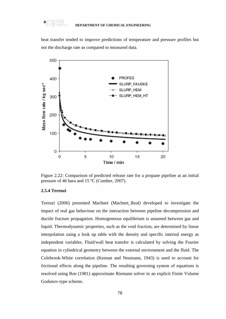
DEPARTMENT OF CHEMICAL ENGINEERING
78
heat transfer tended to improve predictions of temperature and pressure profiles but
not the discharge rate as compared to measured data.
Figure 2.22: Comparison of predicted release rate for a propane pipeline at an initial
pressure of 46 bara and 15 oC (Cumber, 2007).
2.5.4 Terenzi
Terenzi (2006) presented Machnet (Machnet_Real) developed to investigate the
impact of real gas behaviour on the interaction between pipeline decompression and
ductile fracture propagation. Homogeneous equilibrium is assumed between gas and
liquid. Thermodynamic properties, such as the void fraction, are determined by linear
interpolation using a look up table with the density and specific internal energy as
independent variables. Fluid/wall heat transfer is calculated by solving the Fourier
equation in cylindrical geometry between the external environment and the fluid. The
Colebrook-White correlation (Keenan and Neumann, 1943) is used to account for
frictional effects along the pipeline. The resulting governing system of equations is
resolved using Roe (1981) approximate Riemann solver in an explicit Finite Volume
Godunov-type scheme.

DEPARTMENT OF CHEMICAL ENGINEERING
79
Terenzi (2006) also developed a model for the decompression of a pipeline
transporting an ideal gas (Machnet_Ideal) by assuming zero heat transfer and
frictionless flow to derive a similarity solution for the pressure at the exit plane and
the speed of the rarefaction wave.
Machnet_Ideal and Machnet_Real’s predictions were tested by comparison with the
results of tests conducted at the Foothills Pipelines Northern Alberta Burst Test
Facility (NABT) (Picard and Bishnoi, 1987). These tests involved the release of
natural gas (ca. 85 % methane) from pipelines with respective pipeline internal
diameters, pressures and temperatures in the ranges of 1219 to 1422 mm, 7.5 to 8.7
MPa and -18 to +18 oC.
Figure 2.23 shows the variation of the ratio of pressure to initial pressure and void
fraction with expansion wave velocity.
Figure 2.23: Measured and calculated decompression wave speed results of NABT
Test 5 (Picard and Bishnoi, 1987).
The simulated results obtained from Machnet_Ideal and Machnet_Real utilising the
PR and Soave-Redlich-Kwong (SRK) Equations of State were compared with
experimental data. As may be observed, Machnet_Real coupled with either the PR or
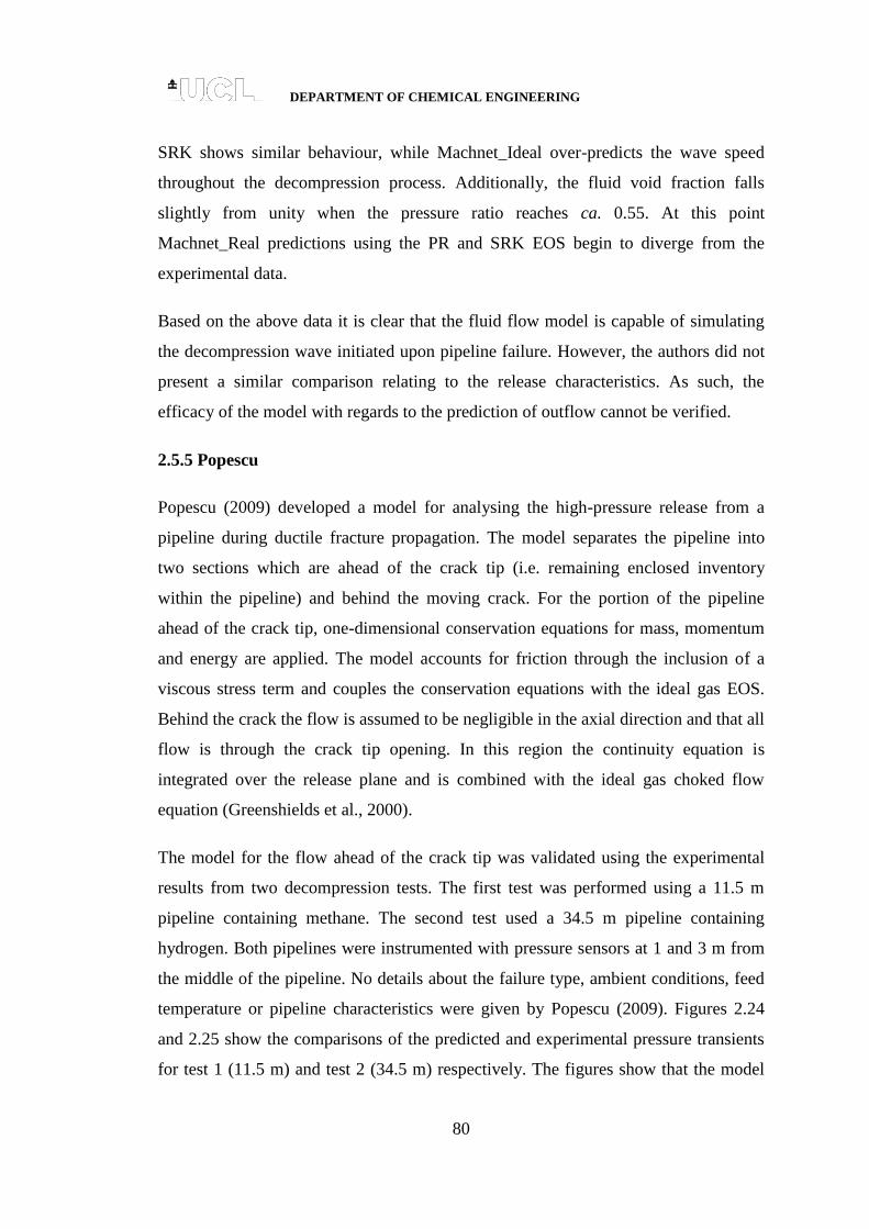
DEPARTMENT OF CHEMICAL ENGINEERING
80
SRK shows similar behaviour, while Machnet_Ideal over-predicts the wave speed
throughout the decompression process. Additionally, the fluid void fraction falls
slightly from unity when the pressure ratio reaches ca. 0.55. At this point
Machnet_Real predictions using the PR and SRK EOS begin to diverge from the
experimental data.
Based on the above data it is clear that the fluid flow model is capable of simulating
the decompression wave initiated upon pipeline failure. However, the authors did not
present a similar comparison relating to the release characteristics. As such, the
efficacy of the model with regards to the prediction of outflow cannot be verified.
2.5.5 Popescu
Popescu (2009) developed a model for analysing the high-pressure release from a
pipeline during ductile fracture propagation. The model separates the pipeline into
two sections which are ahead of the crack tip (i.e. remaining enclosed inventory
within the pipeline) and behind the moving crack. For the portion of the pipeline
ahead of the crack tip, one-dimensional conservation equations for mass, momentum
and energy are applied. The model accounts for friction through the inclusion of a
viscous stress term and couples the conservation equations with the ideal gas EOS.
Behind the crack the flow is assumed to be negligible in the axial direction and that all
flow is through the crack tip opening. In this region the continuity equation is
integrated over the release plane and is combined with the ideal gas choked flow
equation (Greenshields et al., 2000).
The model for the flow ahead of the crack tip was validated using the experimental
results from two decompression tests. The first test was performed using a 11.5 m
pipeline containing methane. The second test used a 34.5 m pipeline containing
hydrogen. Both pipelines were instrumented with pressure sensors at 1 and 3 m from
the middle of the pipeline. No details about the failure type, ambient conditions, feed
temperature or pipeline characteristics were given by Popescu (2009). Figures 2.24
and 2.25 show the comparisons of the predicted and experimental pressure transients
for test 1 (11.5 m) and test 2 (34.5 m) respectively. The figures show that the model

DEPARTMENT OF CHEMICAL ENGINEERING
81
gives good agreement with experimental data following pipeline failure. However, the
speed at which the front of the decompression wave arrives at the probe locations is
slightly over-predicted. This is indicated by the faster pressure drop from the initial
value. Although good agreement is obtained in the pressure profiles presented, the
assumption of ideal gas behaviour means that the model is not applicable to non-ideal
or two-phase mixtures. Further, this assumption leads to an incorrect prediction of the
speed of sound which is essential for the tracking of the expansion wave. In addition,
the performance of the internal flow model is uncertain with respect to long pipelines,
where it is likely that heat transfer and friction may be significant.
Figure 2.24: Comparison of the variation of pressure with time between predicted and
experimental for a 11.5 m pipeline containing methane (Popescu, 2009).
Figure 2.25: Comparison of the variation of pressure with time between predicted and
experimental for a 34.5 m pipeline containing hydrogen (Popescu, 2009).

DEPARTMENT OF CHEMICAL ENGINEERING
82
2.6 Concluding remarks
In this section, the mass, momentum and energy conservation equations for the
transient fluid flow in a pipeline were presented. These were expressed in terms of the
dependent variables pressure, enthalpy/entropy and velocity. The governing system of
conservation equations were shown to be quasi-hyperbolic in character. The
conservation equations coupled with a Cubic Equation of State representing the
foundation of the transient fluid flow model. The various hydrodynamic and
thermodynamic relations for predicting the pertinent fluid properties such as the fluid
speed of sound, the thermodynamic function and the Fanning friction factor were
presented. The formulation and implementation of the Method of Characteristics to
solve the conservation equations governing single/two-phase flow in pipelines was
also described.
Particular attention is paid to the Method of Characteristics as a solution methodology
given its popularity due to its accuracy and robustness. Based on the above reviewed
models, OLGA tended to under-predict the pressure profile, occasionally by
significant margins. For the models SLURP, Terenzi and Popescu, insufficient data
were reported by the researchers to properly assess their suitability for modelling the
transient flow of the high pressurised fluid. For these reasons, the present work will
extend the UCL model, based on the above formulations and review for the study of
transient flow in pressurized pipelines.
In the following chapter 4, special attention will be paid to the design of the
associated pipeline infrastructure in order to avoid large flow fluctuations at the
delivery point of CO2 at the sequestration site. In this chapter 4, the development of a
transient flow model by employing the UCL model which is in turn used as part of the
control strategy for avoiding such phenomena will be studied.

DEPARTMENT OF CHEMICAL ENGINEERING
83
CHAPTER 3:
STUDY OF MULTISTAGE COMPRESSION OF CO2 WITH
IMPURITIES FOR CCS
3.0 Introduction
This chapter deals with multistage compression of impure CO2 streams for CCS
applications. In particular, it covers the description of the types of industrial
compression technologies employed and the types of impurities present in the post-
combustion, pre-combustion and oxy-fuel streams captured from power plants and
industrial processes such as N2, Ar, O2, SO2, H2O, H2S, H2 and etc. This is followed
by the description of the thermodynamic model developed in this work to determine
the total power consumption for multistage compression and intercooler of pure and
impure captured CO2 streams. Using the compression model developed, optimal
multistage compression schemes are determined depending on the outlet pressure
from the separation unit of the captured streams. The calculated power requirements
for compression and intercooler as well as intercooling heat duty for various
compression schemes for particular CO2 mixtures depending on the capture
technologies employed are compared and discussed.
3.1 Technical background
Compression of captured CO2 is the last part of the capture process before
transportation using a pipeline to a geological storage site. The process involves the
use of mature technologies and techniques that are used in the natural gas industry but
with some modifications to suit the properties of CO2 (Wong, 2006). CO2
compression differs from most gas compression due to its high molecular weight,
highly compressible behaviour and encountering its critical point (Witkowski et al.,
2013) where even a small change in temperature or pressure, yields a large change in
density (Oakey et al., 2010). The main reasons for integrating CO2 compression in
CCS are to convert the fluid from the gas phase to the dense phase and also to reach

DEPARTMENT OF CHEMICAL ENGINEERING
84
the technically and economically optimum pressure for pipeline transportation (Gusca
and Blumberga, 2011). However, the compression process requires optimisation due
to its high costs and energy penalty (Notebook, 2011, Pei et al., 2014).
Romeo et al. (2009) have reported about 25 % of the total capital requirements of the
CCS is due to compression equipment costs. Energy requirements for compressing
one tonne of CO2 are about 100-133 kWh (Pei et al., 2014). According to Moore et al.
(2011), the traditional pulverised coal power plant and typical Integrated Gasification
Combine Cycle (IGCC) plant present ca. 27-37 and 13-17 % of the energy penalty of
CCS respectively and the compression part has a significant contribution to this
percentage. The CO2 compression alone reduces the efficiency of a power plant by as
much as 8-12 % from the overall process. In a pulverised coal-fired power plant with
an amine capture based system, the power required for CO2 compression is
approximately 6-12 % of the total plant rating (Witkowski et al., 2013). These values
highlight the necessity for detailed analyses of CO2 compression in the CCS system in
order to minimize both, energetic requirements of the compression and additional
capital requirement for the capture system.
In order to efficiently transport large amounts of CO2, it must be transformed into a
form with high density, meaning that transport in a dense phase or at supercritical
conditions may be considered as shown in figure 3.1.

DEPARTMENT OF CHEMICAL ENGINEERING
85
Figure 3.1: Phase diagram for pure CO2 (Seevam et al., 2008).
A high density is favourable when transporting CO2, as it is easier to move a dense
fluid rather than a gas (Wong, 2006). In the dense phase, the specific volume of CO2
is more than 500 times smaller compared with values at the gas phase (Romeo et al.,
2009). In pipeline systems, CO2 is transported at high pressure above the critical
pressure, most likely in the range of 80-150 bar. The CO2 must be compressed to a
pressure high enough to overcome the frictional and static pressure drops. Typically,
the frictional loss can range from 4 to 50 kPa per km, depending on the pipe diameter,
mass flow rate and the pipe roughness factor. Furthermore, the CO2 should be
delivered at a pressure higher than the critical pressure to avoid two-phase flow and
liquid slugs in the pipeline as well as to prevent liquids in the injection compressor
(Aspelund and Jordal, 2007, Romeo et al., 2009). Hence, in order to maintain the CO2
in the dense phase for the whole pipeline, the inlet pressure of the pipe must be at high
enough pressure above the critical point or booster stations must be installed every
100 to 150 km to compensate for the pressure losses (Wong, 2006).
Many researchers have made important studies in the CCS field, but most of them
focus on the CO2 capture process with compression and transportation receiving
relatively less attention. In particular, Witkowski and Majkut (2012) and Witkowski

DEPARTMENT OF CHEMICAL ENGINEERING
86
et al. (2013) have quantified the power demands for various industrial CO2
compression systems, including conventional 8-stage integrally geared centrifugal
compression, advanced supersonic shockwave compression and multistage
compression combined with subcritical or supercritical liquefaction and pumping. The
authors found that total compression power was not only determined by the
compressor efficiency, but is heavily dependent on thermodynamic processes. These
findings provide relevant data and act as a benchmark since they exemplify how
various industrial compression strategies can be integrated in the CCS system for near
pure CO2 streams.
Furthermore, several studies have examined the opportunities for integration of
compression in CCS and the power generation process. Pei et al. (2014) investigated
coupling CO2 compression with the organic Rankine cycle to re-utilise the heat of
compression in power plant operation, showing that the energy requirements can be
reduced by ca. 17 and 30 % for conventional and shockwave compression,
respectively. Also, Romeo et al. (2009) have shown that utilising heat from the inter-
cooling process in the pre-heating section of steam cycle can give ca. 40 % savings in
compression power. Duan et al. (2013) proposed integrating CO2 compression with
liquefaction using an ammonia absorption refrigeration system powered by the
exhaust heat from steam turbines with a coal-fired power plant that proved to greatly
reduce the power consumed in CO2 compression. Aspelund and Jordal (2007) have
analysed various options for conditioning of CO2 streams, suggesting using expansion
of a fraction of compressed CO2 as a refrigerant in a condenser column for removing
volatile components. While the above studies quantified power requirements for
industrial compression of CO2, their practical application is, however, limited due to
the underlying assumption of negligibly small amounts of impurities in CO2 stream.
The present study evaluates the impact of impurities on power requirements for
compression technologies previously recommended for pure CO2.

DEPARTMENT OF CHEMICAL ENGINEERING
87
3.2 CO2 stream impurities
In practice, the CO2 streams in CCS will contain some impurities with range and
level, mostly depending on the capture technology. Unlike the CO2 streams produced
in post-combustion and pre-combustion captures, the purity of the separated untreated
oxy-fuel CO2 stream is generally much lower, reaching about 75-90 % v/v. The
compositions of CO2 streams captured in oxy-fuel, pre-combustion and post-
combustion captures from coal-burning power plant has recently been reviewed by
Porter et al. (2015). Tables 3.1 and 3.2 lists the impurities present in captured CO2
streams and gives the typical concentrations of the various components.
As can be seen from the data in table 3.1, post-combustion capture (99.66 % v/v of
CO2) has high purity of the CO2 stream along with oxy-fuel distillation process (99.30
% v/v of CO2), followed by pre-combustion (98.07 % v/v of CO2), then the oxy-fuel
double flash process (96.70 % v/v of CO2) and raw oxy-fuel (85 % v/v of CO2)
mixtures. During the oxidation process, NO which is primarily presented as a large
proportion in the NOx composition has converted to NO2 in the presence of oxygen
after a certain residence time (Normann et al., 2013). Early findings by Witkowski
and Majkut (2012) on CO2 compression for the post-combustion mixture did not
evaluate the effect of impurities which kept the level of impure components very low.
However, due to the high amount of impurities present in the pre-combustion and
oxy-fuel streams that generally will affect the energy required for the level of CO2
compression, the effect of these impure components cannot simply be neglected
(IEAGHG, 2011, Kownatzki and Kather, 2011).
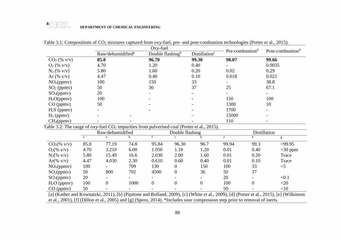
DEPARTMENT OF CHEMICAL ENGINEERING
88
Table 3.1: Compositions of CO2 mixtures captured from oxy-fuel, pre- and post-combustion technologies (Porter et al., 2015).
Oxy-fuel Pre-combustiond Post-combustiond
Raw/dehumidifieda Double flashingb Distillationc
CO2 (% v/v) 85.0 96.70 99.30 98.07 99.66 O2 (% v/v) 4.70 1.20 0.40 - 0.0035
N2 (% v/v) 5.80 1.60 0.20 0.02 0.29
Ar (% v/v) 4.47 0.40 0.10 0.018 0.021
NOx(ppmv) 100 150 33 - 38.8
SO2 (ppmv) 50 36 37 25 67.1
SO3(ppmv) 20 - - - -
H2O(ppmv) 100 - - 150 100
CO (ppmv) 50 - - 1300 10
H2S (ppmv) - - - 1700 -
H2 (ppmv) - - - 15000 -
CH4(ppmv) - - - 110 -
Table 3.2: The range of oxy-fuel CO2 impurities from pulverised coal (Porter et al., 2015).
Raw/dehumidified Double flashing Distillation a e b f c b a b g
CO2(% v/v) 85.0 77.19 74.8 95.84 96.30 96.7 99.94 99.3 >99.95
O2(% v/v) 4.70 3.210 6.00 1.050 1.10 1.20 0.01 0.40 <30 ppm
N2(% v/v) 5.80 15.49 16.6 2.030 2.00 1.60 0.01 0.20 Trace
Ar(% v/v) 4.47 4.030 2.30 0.610 0.60 0.40 0.01 0.10 Trace
NOx(ppmv) 100 - 709 130 0 150 100 33 <5
SO2(ppmv) 50 800 702 4500 0 36 50 37
SO3(ppmv) 20 - - - - - 20 - <0.1
H2O (ppmv) 100 0 1000 0 0 0 100 0 <20
CO (ppmv) 50 - - - - - 50 - <10
[a] (Kather and Kownatzki, 2011), [b] (Pipitone and Bolland, 2009), [c] (White et al., 2009), [d] (Porter et al., 2015), [e] (Wilkinson
et al., 2001), [f] (Dillon et al., 2005) and [g] (Spero, 2014). *Includes sour compression step prior to removal of inerts.

DEPARTMENT OF CHEMICAL ENGINEERING
89
3.2.1 Oxy-fuel combustion capture
Oxy-fuel combustion is becoming a popular option for CO2 capture due to some
specific advantages. This technology is gaining maturity and can be retrofitted to the
existing fleet of modern pulverised coal-fired power plants. In this unit, the fuel is
burned in a mixture of purified oxygen and recycled flue gas from the boiler
containing mainly CO2 and water vapour (Kownatzki and Kather, 2011).
During oxy-fuel capture, the CO2 stream is purified in a sequence of different steps at
increasing pressure levels. In particular, water scrubbing in a direct contact cooler can
be used at ambient pressure to condense water vapour and remove traces of ash,
whereby the removal of some reactive and soluble gases such as SO3 and HCl can be
achieved at pressures of around 15 bar (White et al., 2009). At this stage, the CO2
stream has purity from ca. 70 to 75-85 % v/v (see table 3.2). Also, the ‘sour
compression’ process proposed by Air Products allows for the removal of SOx and
NOx impurities. To further reduce the amount of non-condensable components (such
as O2, N2 and Ar) and achieve CO2 purity of over 95 % v/v, flash-evaporation and
distillation are applied at pressures of around 30 bar (Dillon et al., 2005, White et al.,
2009, Besong et al., 2013). As such, compression is partially integrated in oxy-fuel
CO2 purification, and higher purity CO2 streams can be achieved for transporting and
storage requirements.
3.2.2 Pre-combustion capture
In pre-combustion systems, the removal of CO2 occurs before combustion takes place.
The main concept in this system is coal gasification followed by a water gas shift
reaction and absorption of CO2 (Erlach et al., 2011). CO2 can be removed for storage
purposes and the resultant H2 could be used in fuel cells or in gas turbines to generate
electricity. The process is operated when O2 from the air is separated using an Air
Separation Unit (ASU) before reaction with steam and coal as a fuel in a gasifier or
thermal partial oxidation reactor at 1550 oC and 40 bar to produce syngas such as CO
and H2. The products are extracted in the Selexol-based Acid-Gas Recovery (AGR)
unit to separate H2 from other gases, mainly CO2 using a physical or chemical

DEPARTMENT OF CHEMICAL ENGINEERING
90
absorption process at temperature ca. 30 oC. The clean gas from H2S absorber enters
the CO2 absorber to produce CO2-rich fluid stream at ca. 25 oC, 30-35 bar before
pipeline transportation (Lu et al., 2012).
3.2.3 Post-combustion capture
In post-combustion capture processes, CO2 is separated from flue gas originating from
air-fired combustion. Traditionally, amine-based absorption systems operating at
close to ambient conditions (ca. 1.5 bar and ca. 40 oC (IEAGHG, 2011)) are used to
capture the CO2 from the flue gas, which typically contains only 5-15 % v/v CO2,
with the remaining major components being O2, N2, Ar, H2O, CO, NOX and SO2
(table 3.1). Using amine-based solvents CO2 can be purified to above 99 % v/v. Due
to its relatively high purity, the impact of impurities on thermodynamic properties of
post-combustion CO2 streams is often neglected (Witkowski et al., 2013).
3.2.4 Impact of impurities on CO2 physical properties
The presence of impurities in CO2 streams reduces the effective capacity of CO2
transportation pipelines and storage reservoirs, making the transportation and storage
of industrial-grade CO2 less efficient than for pure CO2. Additionally, the presence of
impurities in CO2 can shift the boundaries in the CO2 phase diagram to higher
pressures, meaning that higher operating pressures are needed to keep the CO2 in the
dense phase. On the other hand, removing impurities from the CO2 stream increases
the capture and purification costs (Holloway and Akai, 2006). Clearly, in order to
minimise the costs of CCS, the costs associated with compression/transportation and
injection of impure CO2 must be optimised in conjunction with the costs of CO2
stream purification.
Of particular importance for compression is that impurities alter the physical
properties and vapour-liquid phase equilibria of CO2 mixtures (Goos et al., 2011,
Ziabakhsh-Ganji and Kooi, 2012) as shown in figure 3.2.

DEPARTMENT OF CHEMICAL ENGINEERING
91
Figure 3.2: Boundaries of VLE region in pressure-temperature phase diagram for pure
CO2, pre-combustion, post-combustion and oxy-fuel streams (85 and 96.70 % v/v
CO2) calculated using PR EoS.
As is shown in figure 3.2, the small amount of impurities in CO2 mixtures produced in
post-combustion and pre-combustion capture has very little impact on the bubble-
point and dew-point curves, which remain close to the saturation curve of pure CO2.
However, in the case of the raw dehumidified oxy-fuel mixture, which carry a
relatively large amount of impurities (15 % v/v), the bubble point and dew point
pressures are remarkably different to the vapour pressure of pure CO2. As such, unlike
the post-combustion and pre-combustion mixtures, the raw oxy-fuel streams can be
expected to have physical properties remarkably different from those of pure CO2. In
addition, from figure 3.2, the liquid vapour phase equilibria and especially the
cricondenbar pressure (i.e. the pressure above which no gas phase can be found in the
fluid) are remarkably different for the three oxy-fuel streams from table 3.1.
Figure 3.2 shows that the range of vapour liquid equilibrium (VLE) data for the
mixtures differs from that for pure CO₂. In particular, the saturation pressures for oxy-
fuel and pre-combustion mixtures differ significantly from the saturation pressure for
pure CO₂ and post-combustion mixture. As can be seen from figure 3.2, the saturation
curves for pure CO₂ and post-combustion CO₂ mixture are nearly identical, as can be

DEPARTMENT OF CHEMICAL ENGINEERING
92
explained by high purity of post-combustion stream and, hence, have a negligible
impact of impurities on the fluid properties. In the case of the pre-combustion and
oxy-fuel mixtures, the purity of the CO₂ stream decreases, and hence the larger
becomes the deviation from the saturation data of pure CO₂.
The data in figure 3.2 show that the presence of impurities has more significant
impact on the bubble point rather than the dew point line. It can be observed that with
the increase in the amount of impurities in the CO₂ mixture, in particular non-
condensable gases, such as N2, O2, Ar and H2, the bubble point line is shifted towards
higher pressures, while the bubble point line temperature is reduced. The effect is
mostly pronounced for the oxy-fuel mixture, which carries the largest amount of
impurities (table 3.1). On the other hand, the impact of impurities in the pre-
combustion and post-combustion mixtures on the bubble point line is relatively small
and becomes significant only for the oxy-fuel mixture.
Figure 3.3 illustrates the effect of compression pressure on the gas-phase and
supercritical fluid density for pure CO₂ and the CO₂ mixtures at the temperature of 38
oC, which corresponds to the typical temperature of CO₂ before compression.
Figure 3.3: The effect of pressure on the density of pure CO₂ and oxy-fuel, pre-
combustion and post-combustion CO₂ mixtures. To = 38 oC.

DEPARTMENT OF CHEMICAL ENGINEERING
93
As can be seen from figure 3.3, at pressures in the range from 1.51 bar to ca. 20 bar,
the density of mixtures from all different capture technologies is about the same. At
pressures above 20 bar, the density increases with pressure and differs considerably
between each capture technology. The density of pure CO₂ and mixture of post-
combustion rose dramatically with the increase of pressure due to the least fraction of
impurities present in the streams. These densities are higher than those of pre-
combustion and oxy-fuel CO₂ mixtures, which would result in higher power
consumption for compression and liquefaction for subsequent pipeline transportation
(Sass et al., 2009).
Figure 3.4 illustrates the effect of pressure on compressibility factor, Z, of pure CO₂
and CO₂ mixtures from oxy-fuel, pre-combustion and post-combustion at the
temperature of 38 oC.
Figure 3.4: Effect of compression pressure on the compressibility factor of pure CO₂ and CO₂ mixtures captured from oxy-fuel, pre-combustion and post-combustion
technology. To = 38 oC
It can be seen that at pressures in the range from 1.51 to ca. 20 bar the compressibility
factor linearly decreases with increasing pressure and is almost independent on the
CO₂ purity. At pressures above 20 bar the compressibility factor for all mixtures
rapidly decreases with pressure. Since the presence of impurities reduces the
molecular weight of the CO₂ mixtures, the pipeline transportation of these mixtures at
a fixed mass flow rate will be characterised by larger pressure drops, to overcome
DEPARTMENT OF CHEMICAL ENGINEERING
94
which higher inlet pressures will be required for less pure CO₂, meaning an increase
in the compression power (Moshfeghian et al., 2008, Tabkhi et al., 2008).
Recently, Aspelund and Jordal (2007), de Visser et al. (2008) and Goos et al. (2011)
have shown that the energy required for CO2 stream compression for pipeline
transportation increases proportionally with the concentration of the gaseous
impurities in CO2 mixtures. These findings thus lend support and provide guidelines
for optimization of compression, transportation and storage processes. However, the
implications of this effect both on the selection of an appropriate compression strategy
for realistic CO2 streams and associated energy penalty costs have not received much
attention.
3.3 Industrial compression technologies
In CCS, compression of a CO2 stream coming from capture/purification facilities for
pipeline transportation and geological storage can be practically achieved using
various different types of industrial compressor, which include conventional
multistage integrally geared compressors, advanced supersonic shockwave
compressors, and compression and pumping with a subcritical or supercritical
liquefaction/refrigeration system. In order to achieve optimal pressure for pipeline
transportation, a number of stages of compression are required.
Thus, compression generally occurs in a number of stages integrated with inter-stage
cooling equipment. Applying coolers after the compression stages will reduce the
power needs for gas compression and therefore the compressor size and total capital
requirement of the system (Romeo et al., 2009, Wong, 2006). The main parameters
affecting the compression power and cooling requirement necessities in the CCS
system are compressor efficiency, pressure ratio and CO2 inlet pressure. The selection
and design of more efficient and economical compression technology are dependent
on the conditioning process which determines the thermodynamic state of the CO2
entering the system.
Table 3.3 summarises the compression technologies adopted in the present study.
These selected technologies have been applied to meet the compression service

DEPARTMENT OF CHEMICAL ENGINEERING
95
requirements depending on inlet and outlet pressures and volumetric flow rate of the
streams (Witkowski and Majkut, 2012). The following gives detailed descriptions of
the compression processes for these options.
Table 3.3: Multistage compression technology option.
Option Compression technology
A Conventional multistage integrally geared centrifugal compressors
B Advanced supersonic shockwave compression
C
D
Multistage compression combined with subcritical liquefaction and
pumping
Multistage compression combined with supercritical liquefaction
and pumping
3.3.1 Option A: Conventional multistage integrally geared centrifugal
compressors
Conventional multistage integrally geared centrifugal compressors, Option A, is the
preferred choice for CO2 compression in the power plant industry (Holloway and
Akai, 2006). This typical compressor has a limited individual pressure ratio in the
range of 1.7-2:1 (Pei et al., 2014). For such pressure ratios, eight stages of the integral
geared compressor are required to achieve an overall pressure ratio of 100:1. In this
option, a group of cylinders is arranged in series with coolers which are provided
between stages in order to reduce the temperature of the compressed gas which
minimises its volume resulting in lower compression work. Due to the significant
reduction in CO₂ volume during the compression process, the setup requires a large
impeller for the first stage and a very small impeller for the last stage (Witkowski and
Majkut, 2012). Normally, centrifugal compressors are the common choice for the
compression of large amounts of CO2. The compressors will have an efficiency of 75-
85 % (Holloway and Akai, 2006). The first two stages must be designed to withstand
the corrosion that is expected due to acidic water. Ideally, the inlet temperature of
each compressor should be the same as it was at the initial condition to achieve the
perfect cooling or isothermal compression.
Selection, sizing and operation of inter-stage coolers are also important
considerations. Intermediate cooling can be done by seawater, freshwater or ambient

DEPARTMENT OF CHEMICAL ENGINEERING
96
air heat exchangers. The rejected intercooling heat may potentially be used to
regenerate the amine solution in the regeneration column of post-combustion capture
applications or to pre-heat the feed-water in the boiler (Witkowski and Majkut, 2012).
In practice, the inlet temperature in each stage is maintained between 35 and 38 oC,
and 110 bar is the minimum discharge pressure to ensure the mixtures are above their
critical pressure (Notebook, 2011). Eight or ten-stage designs are particularly
sensitive to the two-phase region due to the margin between the two-phase condition,
and the compressor stage discharge pressure is in or around the critical point and is
somewhat unpredictable depending on the impurities present (Babcock, 2009).
Due to the compression in every stage being nearly adiabatic, there is an incremental
increase of outlet temperature in CO2 compression. Thus, the energy consumption of
the system is increased. Implementation of the inter-stage cooling can make the
process approach isothermality, which can decrease the power consumption of the
compressor (Duan et al., 2013). Existing CO2 compressors are expensive due to the
overall pressure ratio being high and require stainless steel construction to
accommodate CO2 containing water (Witkowski et al., 2013). This compression
system can be optimized for each stage due to lower volume and higher pressure at
each progressive stage. It is possible to go to different speeds in each stage, so that
very high rpm values about 50,000 rpm can be achieved.
Figure 3.5 shows the schematic diagram of an option A with inter-stage cooling by
recycling the cooling water.

DEPARTMENT OF CHEMICAL ENGINEERING
97
Figure 3.5: Schematic diagram of the compression option A for pure CO2 stream
(adapted from Witkowski and Majkut (2012)).
In the present study, ca. 75 % of efficiency is assumed for each compression stage.
The CO₂ stream is brought to its final pressure through compression sections
intercooled to 38 oC from the compression discharge temperature of ca. 90 oC. Based
on the study by Witkowski and Majkut (2012), ca. 21 % of power savings could be
achieved using option A as compared to an in-line centrifugal compression system. In
the case of pre-combustion and oxy-fuel mixtures, only four stages of compression
system are applied to compress the streams from 15 bar inlet pressure to 151 bar final
pressures. The inlet pressure for each stream is chosen depending on the separation
technology employed for the system (Besong et al., 2013).

DEPARTMENT OF CHEMICAL ENGINEERING
98
3.3.2 Option B: Advanced Supersonic Shockwave Compression
Option B, Advanced Supersonic Shockwave Compression is uniquely suited for
compression of large volumes of CO₂, offering higher compression efficiency of
more than 80 % (Kidd and Miller, 2012). This compression option uses high pressure
ratios ca. 10-12:1 per stage and has a more compact design and lower capital cost as
compared to traditional centrifugal compression (option A). It is expected that using
one or two stages of supersonic compression, that a compressor energy system will do
the same work as option A (Kidd and Miller, 2011). A rotating disk in this
compressor will operate at high peripheral speeds, producing air velocities above the
speed of sound and creating shock waves that efficiently compress the CO2. However,
because of the high compression ratio applied, even using better performance of the
compressor strategy, the power consumption is still tremendous (Duan et al., 2013).
This option is a viable alternative to refrigeration, liquefaction and liquid pumping,
while avoiding the cost and complexities of the refrigeration plant (Kidd and Miller,
2012). As an additional benefit, it provides the high discharge temperature of ca. 279
oC, which can be made useful, e.g. pre-heat the boiler feed-water or re-generate amine
solutions in post-combustion capture applications (Witkowski and Majkut, 2012).
Figure 3.6 shows the schematic illustration of the option B used in this study.
Figure 3.6: Schematic illustration of the industrial compression option B for pure CO2
stream (adapted from Witkowski and Majkut (2012)).
The compression process of CO2 begins at an initial pressure of 1.51 bar and
continues in the first section at the low pressure (LP) compressor to a pressure of 15.1
bar. The gas is then cooled to 38 oC and is further compressed in the last section of a
high pressure (HP) compressor to a pressure of 151 bar in supercritical condition.

DEPARTMENT OF CHEMICAL ENGINEERING
99
However, in the case of pre-combustion and oxy-fuel mixtures with 15 bar inlet
pressure, they are compressed in a single LP compression system to the final pressure.
3.3.3 Option C: Multistage compression combined with subcritical liquefaction
and pumping
In this option C, the pump is used at an intermediate pressure rather than a compressor
to bring the dense phase to final conditions suitable for pipeline transportation. The
underlying premise of the liquefaction approach is that liquid pumps require
significantly less power to raise pressure and are considerably less expensive than gas
compressors (Duan et al., 2013). Depending on the cooling water temperature, using
pumps to build up the fluid pressure from 65 to 150 bar allows a saving of ca. 10-15
% of the power spent in conventional gas-phase compression (Holloway and Akai,
2006). The analysis by Witkowski and Majkut (2012) showed that compared with the
conventional multistage compression process (option A), option C allowed reduction
in the compression power requirement by ca. 20.4 %.
Figure 3.7 shows the schematic diagram of the multistage compression integrated
with the pumping system.

DEPARTMENT OF CHEMICAL ENGINEERING
100
Figure 3.7: Schematic diagram of the compression option C for pure CO2 (adapted
from Witkowski and Majkut (2012)).
CO2 is converted into liquid at lower pressure using a method of combining the multi-
stage compression and lower temperature cooling. Then, the liquefied CO2 is
compressed into a specified pressure using a pump. In this study, six stages of
compression are used to bring the pure CO2 gas to a subcritical pressure of 62.54 bar,
while for pre-combustion and oxy-fuel mixtures, three stages of compression are
employed.
Liquefaction of CO2 at subcritical pressure can maximise the contributions of the low-
energy intensive pump (Pei et al., 2014). However, requiring a large amount of
refrigeration energy for liquefaction purposes is the main drawback in this
compression strategy (Duan et al., 2013, Witkowski et al., 2013).

DEPARTMENT OF CHEMICAL ENGINEERING
101
3.3.4 Option D: Multistage compression combined with supercritical liquefaction
and pumping
In this compression option, liquefaction of the CO2 stream is done at pressures
slightly above the critical pressure, assuring the minimisation of the energy
consumption of the compression system (Witkowski and Majkut, 2012, Pei et al.,
2014). Based on the study by Witkowski and Majkut (2012), ca. 14.6 % of power
reduction for compression of pure CO2 is reported when using a multistage
compression combined with supercritical liquefaction and subsequent pumping, as
compared to the conventional multistage compression option (option A). In this
option D as depicted in figure 3.8, CO2 is brought to just above its critical pressure
through seven compression sections intercooled to 38 oC by water at ambient
conditions.
Figure 3.8: Schematic diagram of the compression option D for pure CO2 (adapted
from Witkowski and Majkut (2012)).

DEPARTMENT OF CHEMICAL ENGINEERING
102
Subsequent cooling results in the liquefaction of the CO2 at the compressor outlet
pressure of 85.49 bar, after which a pump is used to bring the dense fluid to the final
pressure.
3.4 Methodology: Thermodynamic analysis
In the present study, a thermodynamic analysis method is developed and applied to
determine the thermodynamic state of the CO2 stream and to quantify the compression
power consumption for each step of a multistage compression process. The model
accounts for isentropic efficiencies of compression/pumping stages and thermal
efficiencies of heat exchange in isobaric intercoolers.
In particular, the total power required in the N-stage compression/pumping is
calculated as:
N
i
P
P sicomp
comp
outi
ini
dpGW
1 , 3.1
where, G and are the mass flow rate and the density of CO2 stream, respectively,
while in
ip ,out
ip and icomp, are respectively the inlet and outlet pressures and isentropic
efficiency of the thi compression stage. The subscript s denotes isentropic
compression.
Using the first law of thermodynamics,
dpTdsdh and assuming isentropic
compression, equation 3.1 may be written as:
in
i
out
i
N
i icomp
comp hhGW 1 ,
1
3.2
where in
ih and out
ih are enthalpies of the stream at the suction (in) and discharge (out)
of the thi compression stage.
The total cooling duty associated with removing the heat of compression and possibly
liquefying the CO2 stream is given by Duan et al. (2013):

DEPARTMENT OF CHEMICAL ENGINEERING
103
N
i
in
i
out
icool hhGQ2
1 3.3
In the present study, the compression power and cooling duty are calculated as
specific values per tonne of CO2 captured, as commonly considered when estimating
‘costs of CO2 avoided’ (McCoy and Rubin, ). The corresponding specific
compression power and cooling duty are defined as:
N
i
in
i
out
i
icompCO
m
COCO
comp
comp hhM
M
G
Ww
1 ,
11
222
3.4
N
i
in
i
out
i
CO
m
COCO
coolcool hh
M
M
G
2
1
222
1
3.5
where 2COG and
2CO are respectively the mass flow rate and mole fraction of CO2
component in a mixture, while mM and 2COM are molecular weights of the mixture
and CO2, respectively.
While in previous studies, the power demand for inter-stage cooling was generally
assumed to be small with the demand for liquefaction characterised in terms of the
cooling duty (Witkowski et al., 2013, Posch and Haider, 2012), the present analysis
uses a simple and effective thermodynamic model based on Carnot refrigeration cycle
for estimation of the power demand for cooling/liquefaction of the CO2 stream. In this
model, the CO2 cooling power demand is associated with the work spent in an ideal
compression refrigeration cycle when moving the heat from a coolant evaporation
temperature, evT to a condensation temperature, condT (Jobson, 2014):
ev
evcond
cool
coolcool
T
TTqw
3.6
where cool is the efficiency of refrigeration process. In the present study, the coolant
evaporation temperature, evT is set to be 5 oC less than the CO2 stream cooling
temperature, while the condensation temperature, condT , is assumed to be 38 oC. This
model, advantageously, does not involve specification of the type of refrigerant, hence

DEPARTMENT OF CHEMICAL ENGINEERING
104
enabling the comparison of the cooling and liquefaction power consumption for
various multistage compression strategies.
Using equations 3.1 to 3.5 require knowledge of the fluid thermodynamic properties
of CO2 mixtures, namely enthalpies, which can be calculated using dedicated models
as described in the next section. The integral in equation 3.1 defines the compression
work done on the fluid which is valid irrespective of the CO2 mixture phase state, and
hence can be applied to evaluate compression work for the gas and pumping works
for the liquid. This integral is evaluated numerically using a 15-point Gauss-Kronrod
quadrature rule in QUADPACK library (Piessens, 1983).
3.5 Properties of CO2 mixtures with impurities
In order to evaluate the enthalpies in equations 3.2-3.5, Peng-Robinson Equation of
State (PR EOS) (Peng and Robinson, 1976) is used in the present study as one of the
most computationally efficient equations for the modelling of the vapour-liquid
behaviour of CO2 and its mixtures with various components (Seevam et al., 2008,
Zhao and Li, 2014, Li and Yan, 2009). In particular, the fluid density, , is calculated
from the PR EOS:
22
2
211cc
c
c bb
a
b
RTP
3.7
where P and T are respectively the pressure and temperature, while ac, α and bc are the
model parameters which are defined as:
2
22
45724.0c
c
cP
TRa 3.8
c
c
cP
RTb 07780.0 3.9
25.0
1
cT
T 3.10
226922.05422.137464.0 3.11

DEPARTMENT OF CHEMICAL ENGINEERING
105
Here Pc and Tc are respectively the fluid critical pressure and temperature, and ω is
the fluid acentric factor.
In the case of a mixture, ca , α and cb are respectively evaluated using the appropriate
linear mixing rules and combining rules (Sandler, 2007, Wei and Sadus, 2000, Zhao
and Li, 2014):
jcic
N
i
N
j
ijjic aayya
1 1
1 3.12
N
i
ciic byb1
3.13
where ica ,
jca and cib are the PR EOS parameters for the thi and thj
components, while ij is the parameter characterising interaction between
components i and j in the mixture. The ij is estimated using correlations proposed
by Nishiumi and Arai (1988) and Valderrama and Reyes (1983) for binary mixtures
involving hydrocarbons, inert gas, polar components and hydrogen. Table 3.4 lists the
binary interaction parameter ij calculated for the CO2 and various impurities relevant
to the study.
Table 3.4: Values of the interaction parameter, ij for the various binary mixtures
(Valderrama and Reyes, 1983, Nishiumi and Arai, 1988).
CO2 N2 H2 O2 CO H2S SO2 H2O CH4 Ar
CO2 0 -0.02 0.34 0 0 0.11 0 0 0.11 0
N2 -0.02 0 0.05 0 0 0.15 0 0 0.04 0
H2 0.34 0.05 0 0 0.07 0.14 0.33 0.28 -0.02 -0.05
O2 0 0 0 0 0 0 0 0 0 0
CO 0 0 0.07 0 0 0 0 0 0 0
H2S 0.11 0.15 0.14 0 0 0 0 0 0.08 0
SO2 0 0 0.33 0 0 0 0 0 0 0
H2O 0 0 0.28 0 0 0 0 0 0.51 0
CH4 0.11 0.04 -0.02 0 0 0.08 0 0.51 0 0
Ar 0 0 -0.05 0 0 0 0 0 0 0

DEPARTMENT OF CHEMICAL ENGINEERING
106
In particular, to calculate the fluid enthalpy, h and temperature at a given pressure and
entropy, s, pressure-entropy flash calculations are performed by solving
simultaneously the following two equations (Sandler, 2007):
c
c
c
c
c
IG
PbZRT
PbZRT
b
adT
adT
ZRThh21
21ln
221
3.14
c
cc
c
cIG
PbZRT
PbZRT
dt
da
bRT
pbZRss
21
21ln
22
1ln 3.15
where IGh and IGs are respectively the fluid enthalpy and entropy in the ideal gas state.
While RT
pz is the fluid compressibility. The derivative
dT
ad c is defined as:
cc
cc
TTP
TR
dT
ad
22
45724.0 . 3.16
In the present study, the above properties (equations 3.14 and 3.15) are calculated
using PR EOS implemented in REFPROP v.9.1 (Lemmon and Huber, 2010).
3.6 Results and Discussions: Multistage compression of CO2 streams
containing impurities
As mentioned earlier in section 3.1, the general objective of the study is to evaluate
the previously recommended compression options by Witkowski and Majkut (2012)
for the case of pre-combustion and oxy-fuel streams. As the cost of compression
much depends on the power consumption, the primary objective is to compare the
power demands for compression of pure CO2 with pre-combustion and oxy-fuel CO2
streams. To make such a comparison, the thermodynamic analysis method as
described in sections 3.4 and 3.5 is used where the power demand for compression is
calculated using the rigorous equations accounting for real fluid behaviour of CO2 and
its mixtures with impurities.
During multistage compression different fluid phases (gas or liquid) at certain stages
of compression are encountered. Impurities can affect the vapour liquid equilibrium of
CO2. As such, another objective of this study is to examine how the difference in
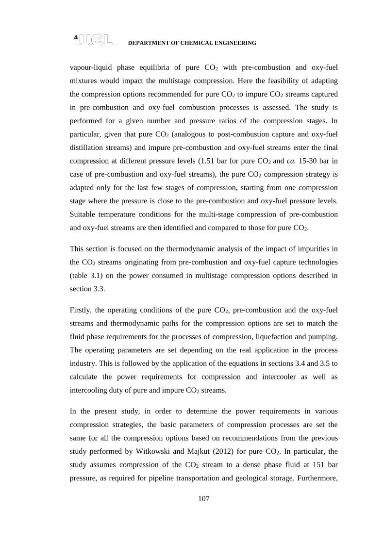
DEPARTMENT OF CHEMICAL ENGINEERING
107
vapour-liquid phase equilibria of pure CO2 with pre-combustion and oxy-fuel
mixtures would impact the multistage compression. Here the feasibility of adapting
the compression options recommended for pure CO2 to impure CO2 streams captured
in pre-combustion and oxy-fuel combustion processes is assessed. The study is
performed for a given number and pressure ratios of the compression stages. In
particular, given that pure CO2 (analogous to post-combustion capture and oxy-fuel
distillation streams) and impure pre-combustion and oxy-fuel streams enter the final
compression at different pressure levels (1.51 bar for pure CO2 and ca. 15-30 bar in
case of pre-combustion and oxy-fuel streams), the pure CO2 compression strategy is
adapted only for the last few stages of compression, starting from one compression
stage where the pressure is close to the pre-combustion and oxy-fuel pressure levels.
Suitable temperature conditions for the multi-stage compression of pre-combustion
and oxy-fuel streams are then identified and compared to those for pure CO2.
This section is focused on the thermodynamic analysis of the impact of impurities in
the CO2 streams originating from pre-combustion and oxy-fuel capture technologies
(table 3.1) on the power consumed in multistage compression options described in
section 3.3.
Firstly, the operating conditions of the pure CO2, pre-combustion and the oxy-fuel
streams and thermodynamic paths for the compression options are set to match the
fluid phase requirements for the processes of compression, liquefaction and pumping.
The operating parameters are set depending on the real application in the process
industry. This is followed by the application of the equations in sections 3.4 and 3.5 to
calculate the power requirements for compression and intercooler as well as
intercooling duty of pure and impure CO2 streams.
In the present study, in order to determine the power requirements in various
compression strategies, the basic parameters of compression processes are set the
same for all the compression options based on recommendations from the previous
study performed by Witkowski and Majkut (2012) for pure CO2. In particular, the
study assumes compression of the CO2 stream to a dense phase fluid at 151 bar
pressure, as required for pipeline transportation and geological storage. Furthermore,
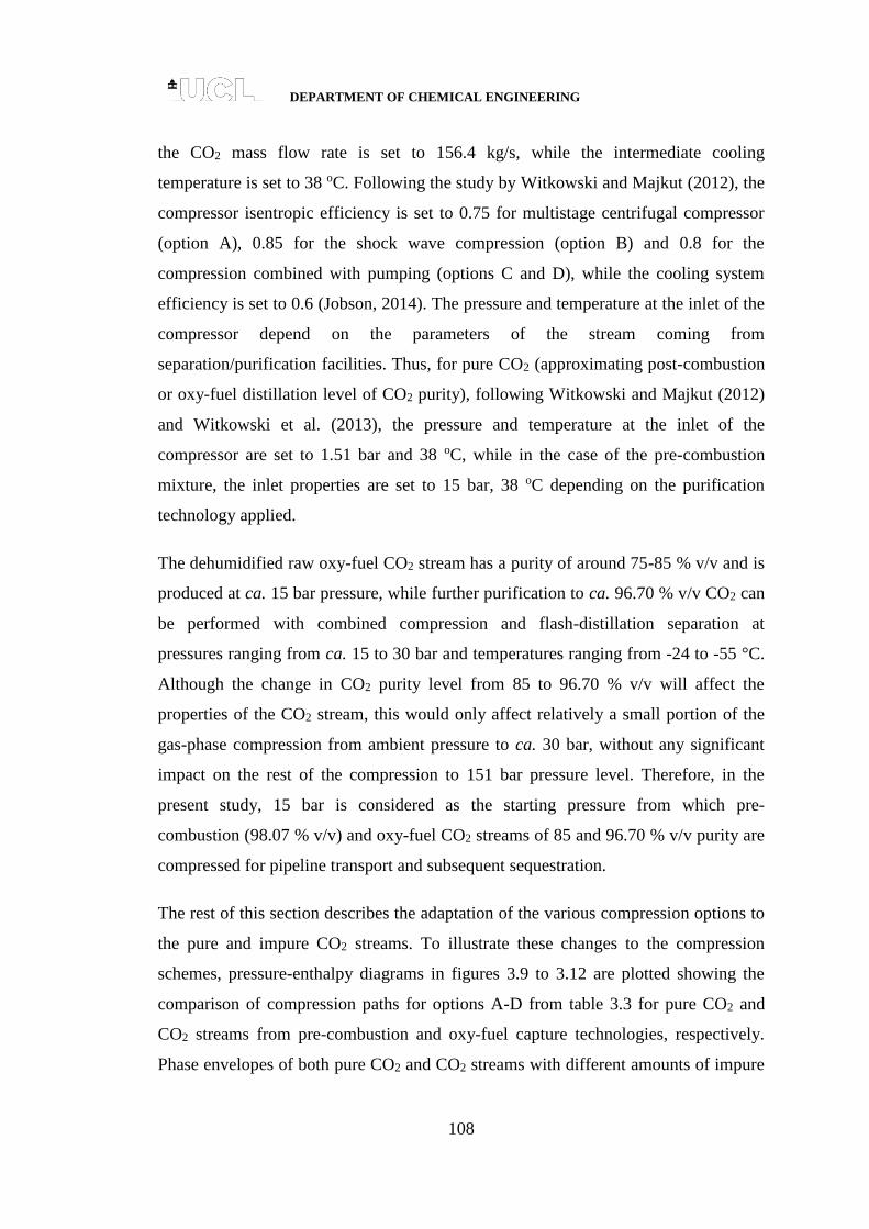
DEPARTMENT OF CHEMICAL ENGINEERING
108
the CO2 mass flow rate is set to 156.4 kg/s, while the intermediate cooling
temperature is set to 38 oC. Following the study by Witkowski and Majkut (2012), the
compressor isentropic efficiency is set to 0.75 for multistage centrifugal compressor
(option A), 0.85 for the shock wave compression (option B) and 0.8 for the
compression combined with pumping (options C and D), while the cooling system
efficiency is set to 0.6 (Jobson, 2014). The pressure and temperature at the inlet of the
compressor depend on the parameters of the stream coming from
separation/purification facilities. Thus, for pure CO2 (approximating post-combustion
or oxy-fuel distillation level of CO2 purity), following Witkowski and Majkut (2012)
and Witkowski et al. (2013), the pressure and temperature at the inlet of the
compressor are set to 1.51 bar and 38 oC, while in the case of the pre-combustion
mixture, the inlet properties are set to 15 bar, 38 oC depending on the purification
technology applied.
The dehumidified raw oxy-fuel CO2 stream has a purity of around 75-85 % v/v and is
produced at ca. 15 bar pressure, while further purification to ca. 96.70 % v/v CO2 can
be performed with combined compression and flash-distillation separation at
pressures ranging from ca. 15 to 30 bar and temperatures ranging from -24 to -55 °C.
Although the change in CO2 purity level from 85 to 96.70 % v/v will affect the
properties of the CO2 stream, this would only affect relatively a small portion of the
gas-phase compression from ambient pressure to ca. 30 bar, without any significant
impact on the rest of the compression to 151 bar pressure level. Therefore, in the
present study, 15 bar is considered as the starting pressure from which pre-
combustion (98.07 % v/v) and oxy-fuel CO2 streams of 85 and 96.70 % v/v purity are
compressed for pipeline transport and subsequent sequestration.
The rest of this section describes the adaptation of the various compression options to
the pure and impure CO2 streams. To illustrate these changes to the compression
schemes, pressure-enthalpy diagrams in figures 3.9 to 3.12 are plotted showing the
comparison of compression paths for options A-D from table 3.3 for pure CO2 and
CO2 streams from pre-combustion and oxy-fuel capture technologies, respectively.
Phase envelopes of both pure CO2 and CO2 streams with different amounts of impure
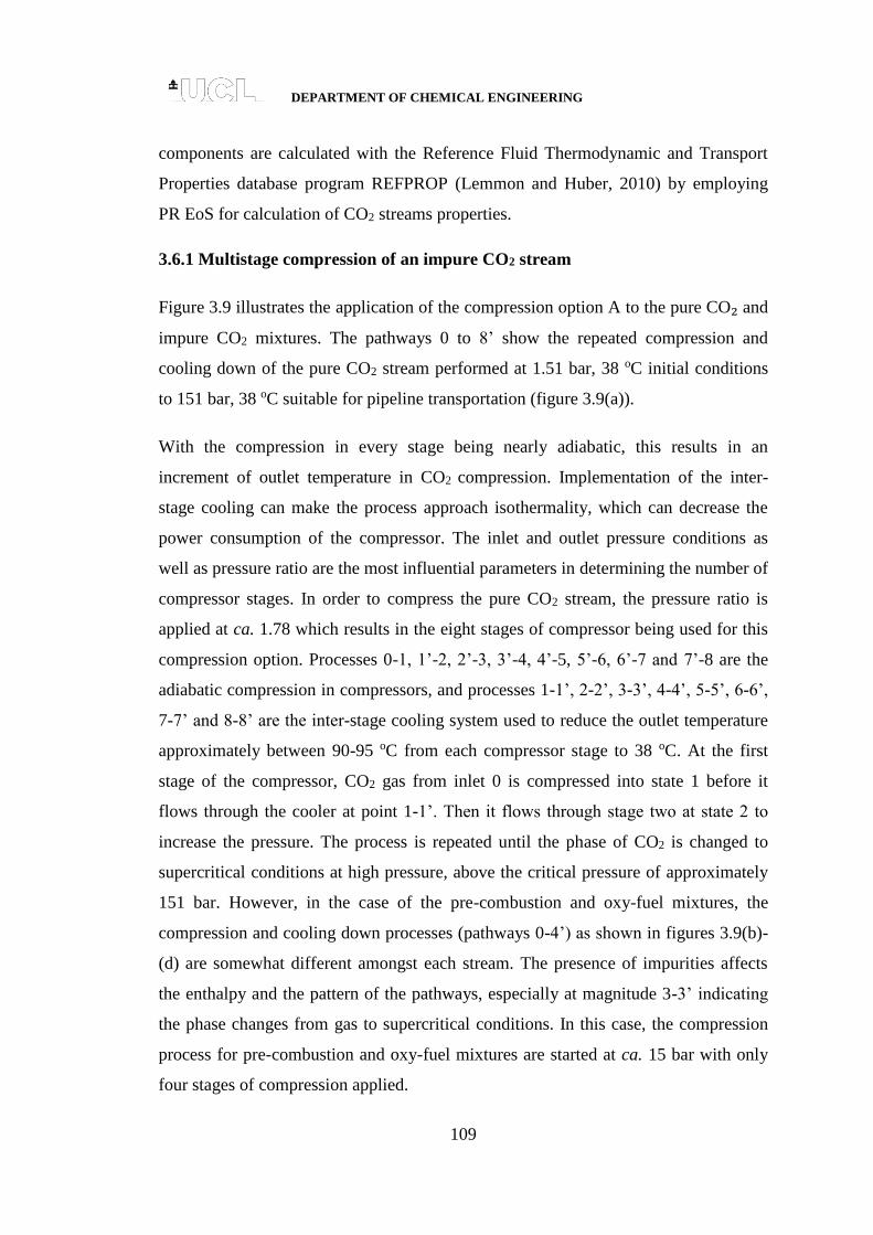
DEPARTMENT OF CHEMICAL ENGINEERING
109
components are calculated with the Reference Fluid Thermodynamic and Transport
Properties database program REFPROP (Lemmon and Huber, 2010) by employing
PR EoS for calculation of CO2 streams properties.
3.6.1 Multistage compression of an impure CO2 stream
Figure 3.9 illustrates the application of the compression option A to the pure CO₂ and
impure CO2 mixtures. The pathways 0 to 8’ show the repeated compression and
cooling down of the pure CO2 stream performed at 1.51 bar, 38 oC initial conditions
to 151 bar, 38 oC suitable for pipeline transportation (figure 3.9(a)).
With the compression in every stage being nearly adiabatic, this results in an
increment of outlet temperature in CO2 compression. Implementation of the inter-
stage cooling can make the process approach isothermality, which can decrease the
power consumption of the compressor. The inlet and outlet pressure conditions as
well as pressure ratio are the most influential parameters in determining the number of
compressor stages. In order to compress the pure CO2 stream, the pressure ratio is
applied at ca. 1.78 which results in the eight stages of compressor being used for this
compression option. Processes 0-1, 1’-2, 2’-3, 3’-4, 4’-5, 5’-6, 6’-7 and 7’-8 are the
adiabatic compression in compressors, and processes 1-1’, 2-2’, 3-3’, 4-4’, 5-5’, 6-6’,
7-7’ and 8-8’ are the inter-stage cooling system used to reduce the outlet temperature
approximately between 90-95 oC from each compressor stage to 38 oC. At the first
stage of the compressor, CO2 gas from inlet 0 is compressed into state 1 before it
flows through the cooler at point 1-1’. Then it flows through stage two at state 2 to
increase the pressure. The process is repeated until the phase of CO2 is changed to
supercritical conditions at high pressure, above the critical pressure of approximately
151 bar. However, in the case of the pre-combustion and oxy-fuel mixtures, the
compression and cooling down processes (pathways 0-4’) as shown in figures 3.9(b)-
(d) are somewhat different amongst each stream. The presence of impurities affects
the enthalpy and the pattern of the pathways, especially at magnitude 3-3’ indicating
the phase changes from gas to supercritical conditions. In this case, the compression
process for pre-combustion and oxy-fuel mixtures are started at ca. 15 bar with only
four stages of compression applied.

DEPARTMENT OF CHEMICAL ENGINEERING
110
(a) (b)
(c) (d)
Figure 3.9: Phase envelope boundaries and thermodynamic paths for compression of pure CO2 (a), 85 % v/v CO2 purity (b), 96.70 % v/v
CO2 purity (c) from oxy-fuel captures and pre-combustion mixture (d) using compression option A (dashed lines).

DEPARTMENT OF CHEMICAL ENGINEERING
111
The effect of impure components in the pre-combustion and oxy-fuel streams (figures
3.9(b)-(d)) lead to a change in the phase envelope boundary (solid line) with the lifted
bubble and dew point lines (dash line) located at higher pressure and also reducing the
supercritical region by influencing the tolerance limit of the transportation pressure.
Figure 3.10 illustrates the thermodynamic compression paths for option B, achieved
using the advanced supersonic shockwave compression with a pressure ratio of 10 per
stage. In the case of pure CO₂, the 2-stage compressor which involves Low Pressure
(LP) and High Pressure (HP) stages is used to increase the pressure from 1.51 to 151
bar at discharge (figure 3.10(a)), while for the pre-combustion and oxy-fuel mixtures,
the inlet pressures are 15 bar and hence only single stage compression is used as
shown in figures 3.10(b)-(d).
Applying only the LP stage of compression option B to compress the pre-combustion
and oxy-fuel mixtures is practically feasible in CCS applications which significantly
reduce the total capital costs of the overall process (Baldwin and Williams, 2009).
The intercooling system is applied to reduce the temperature after the compression
from ca. 279 oC back down to 38 oC.

DEPARTMENT OF CHEMICAL ENGINEERING
112
(a) (b)
(c) (d)
Figure 3.10: Phase envelope boundaries and thermodynamic paths for compression of pure CO2 (a), 85 % v/v CO2 purity (b), 96.70 %
v/v CO2 purity (c) from oxy-fuel captures and pre-combustion mixture (d) using compression option B (dashed lines).

DEPARTMENT OF CHEMICAL ENGINEERING
113
In figure 3.11, the thermodynamic compression paths are shown in compression
option C, which combines multistage compression with pumping following the
liquefaction of CO₂ at subcritical pressures. In this option, the 6-stage and 3-stage
compression processes are respectively adapted for pure CO2 and the impure CO2
streams to compress the fluid before liquefaction and pumping to the final pressure of
151 bar with the pressure ratio of ca. 1.86 applied. The final temperature for pure CO2
at the outlet pumping station is ca. 23 oC while for impure CO2 streams, the final
temperatures are decreased with increasing impurities from 20 oC for pre-combustion
carrying 98.07 % v/v purity, followed by 15 and -67 oC for 96.70 and 85 % v/v purity
of CO2, respectively.
As mentioned in section 3.3.3, the advantage of option C comes from the fact that
using pumps is cheaper than operating compressors. However, in order to use this
advantage, the liquefaction should be achieved at intermediate pressures below the
discharge pressure of the compressor (151 bar) without a significant rise in the
process cost. Thus, Witkowski and Majkut (2012) and Holloway and Akai (2006)
have recommended liquefaction at a pressure around 62.53 bar, which corresponds to
the bubble point temperature of 23 oC for pure CO2. In the case of oxy-fuel and pre-
combustion streams with a purity of 96.70 and 98.07 % v/v, the bubble point
temperatures and pressures are respectively at ca. 15 oC, 62.53 bar and 20 oC, 62.53
bar.
In comparison, the oxy-fuel mixture with 85 % v/v of pure CO2 has the bubble point
temperature of ca. -67 oC which is much lower than the other CO2 streams. As such,
liquefaction of this CO2 stream at 62.53 bar using room-temperature utility streams is
not practically feasible and would require using refrigeration systems.

DEPARTMENT OF CHEMICAL ENGINEERING
114
(a) (b)
(c) (d)
Figure 3.11: Phase envelope boundaries and thermodynamic paths for compression of pure CO2 (a), 85 % v/v CO2 purity (b), 96.70 %
v/v CO2 purity (c) from oxy-fuel capture and pre-combustion mixtures (d) using compression option C (dashed lines).

DEPARTMENT OF CHEMICAL ENGINEERING
115
The presence of impurities significantly affects the properties compared to pure CO2
with changes in the critical pressure and temperature of the stream. In such cases, the
liquefaction would require using cryogenic coolants, increasing the cost of the whole
process.
Figure 3.12 shows the thermodynamic paths in the case of compression option D,
where 7-stage of compression are combined with supercritical liquefaction and
pumping to compress the pure CO2. In the case of the oxy-fuel mixture with 85 % v/v
CO2 purity (figure 3.12(b)), four stages of compression are used, while for 96.70 and
98.07 % v/v purity, three stages of compression are respectively adapted before
pumping for supercritical liquefaction to discharge conditions as shown in figures
3.12(c) and (d). The supercritical liquefaction pressures are chosen to be just above
the maximum saturation pressure of the streams, i.e. 85.49 bar for pure CO₂, 96.70
and 98.07 % v/v purity of CO2 streams and 115 bar for the 85 % v/v purity from oxy-
fuel mixture. The corresponding ‘liquefaction’ temperatures are ca. 15 oC for pure
CO₂ and ca. 10 oC for 96.70 and 98.07 % v/v purity of the CO2 streams,
respectively, while ca. 5 oC for the oxy-fuel mixture with 85 % v/v purity. As can be
seen in figure 3.12(a), the pressure of pure CO2 is increased slightly above the critical
pressure (73.77 bar) using seven stages of compression with pressure ratio of ca. 1.78
applied before liquefaction using water as a cooling medium. Meanwhile, 3-stage
compression is adapted for both 96.70 and 98.07 % v/v CO2 purity. In comparison,
the oxy-fuel mixture with 85 % v/v purity is compressed to the supercritical
liquefaction pressure of 115 bar through four compression stages followed by
liquefaction and pumping to 151 bar for pipeline transportation.
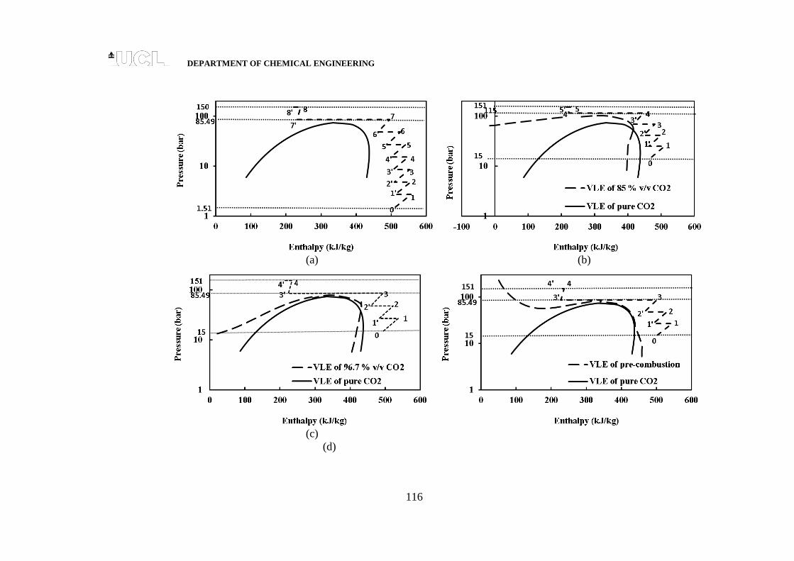
DEPARTMENT OF CHEMICAL ENGINEERING
116
(a) (b)
(c)
(d)

DEPARTMENT OF CHEMICAL ENGINEERING
117
Figure 3.12: Phase envelope boundaries and thermodynamic paths for compression of pure CO2 (a), 85 % v/v CO2 purity (b), 96.70 %
v/v CO2 purity (c) from oxy-fuel capture and pre-combustion mixtures (d) using compression option D (dashed lines).

DEPARTMENT OF CHEMICAL ENGINEERING
118
3.6.2 Multistage compression power demands
Table 3.5 summarises the results of the calculation of the total power of compression
and intercooling as well as cooling duty for 156.4 kg/s of pure CO2 and impure CO2
streams. The presented results are calculated using the equations in sections 3.4 and
3.5 for the multistage compression options A, B, C and D as listed in table 3.3. To
enable comparison for streams originating at different initial pressures (1.51 bar for
pure CO2 and 15 bar in case of pre-combustion and oxy-fuel mixtures), the analysis is
performed starting from 15 bar and 38 oC.
Table 3.5: Compression power, cooling duty and cooling power in multistage
compression/intercooling of various CO2 streams (table 3.1), evaluated for different
compression options.
CO2 Compression technology options
(% v/v) A B C D
Compression power (kWh/tonneCO2)
Oxy-fuel:
Raw dehumidified 85.00 51 64 36 40
Double flashing 96.70 42 55 32.5 35
Pre-combustion 98.07 41 54 32.5 34.5
Pure CO2 100 39 53 32 34
Cooling duty (kWh/tonneCO2)
Oxy-fuel:
Raw dehumidified 85.00 88.78 105 145 112
Double flashing 96.70 90.5 106 102 98
Pre-combustion 98.07 90.5 106 102 98
Pure CO2 100 90.9 107 97 97
Cooling power (kWh/tonneCO2)
Oxy-fuel:
Raw dehumidified 85.00 2.42 2.86 114.5 25.9
Double flashing 96.70 2.47 2.89 16.8 19.2
Pre-combustion 98.07 2.47 2.89 13.6 19.2
Pure CO2 100 2.47 2.89 11.1 15.9
In figures 3.13(a), (b), (c) and (d), the data from table 3.5 are plotted, showing
respectively the compression power, cooling duty, cooling power and total power
consumption of compression power and cooling power of compression options A, B,

DEPARTMENT OF CHEMICAL ENGINEERING
119
C and D for pure CO2 and impure CO2 streams captured from different capture
technologies employed.
(a)
(b)
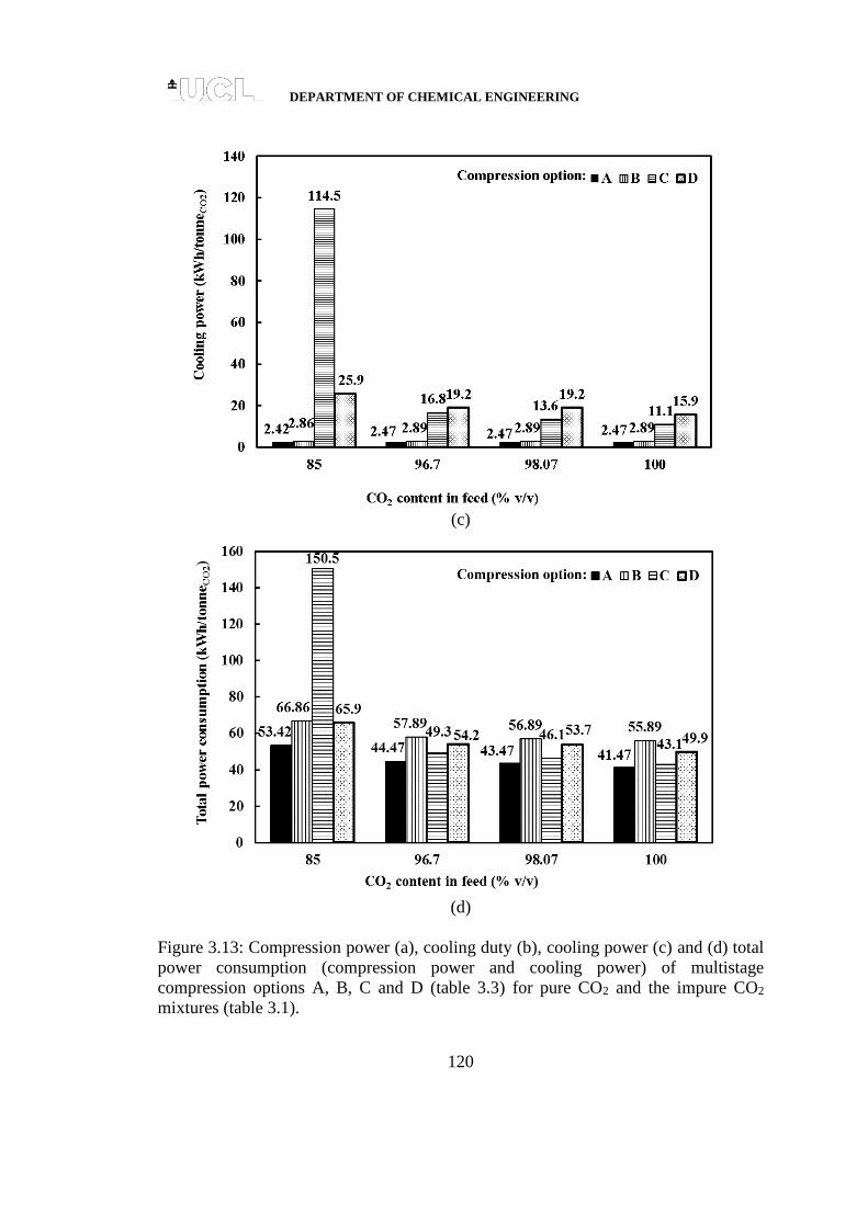
DEPARTMENT OF CHEMICAL ENGINEERING
120
(c)
(d)
Figure 3.13: Compression power (a), cooling duty (b), cooling power (c) and (d) total
power consumption (compression power and cooling power) of multistage
compression options A, B, C and D (table 3.3) for pure CO2 and the impure CO2
mixtures (table 3.1).

DEPARTMENT OF CHEMICAL ENGINEERING
121
As can be seen from the results illustrated in figures 3.13(a), (b) and (d), the presence
of impurities in the CO2 stream affects both the compression power demand and
cooling duty for multistage compression systems. The energy requirements in the
range of ca. 32-53 kWh/tonneCO2 for the compression options adapted in this study for
pure CO2 stream at 15 bar initial pressures are in agreement with the previous studies
by Walspurger and Dijk (2012), IEAGHG (2011) and Witkowski et al. (2013). The
power demand for compression of pure CO2 using supersonic compressors (option B)
is estimated to be ca. 35 % higher than that for the centrifugal compression (option
A). On the other hand using liquefaction and pumping (options C and D) reduces the
compression power demands by ca. 18 and 13 % when compared to multistage
centrifugal compressors (option A).
Also, the results in figure 3.13(a) show nearly equal power demands for compression
of the double-flash 96.7 % v/v purity oxy-fuel and the 98.07 % v/v purity pre-
combustion streams. This can be attributed to the fact that the pre-combustion CO2
stream contains 1.5 % v/v of hydrogen (table 3.1), which is relatively small compared
to 3.2 % v/v of volatiles (N2, O2 and Ar) found in oxy-fuel double-flash stream, but
has stronger effect on the physical properties of the fluid, particularly the density and,
hence, the compression power.
Remarkably, the results in figures 3.13(a) and (b) indicate that multistage
compression is characterised by a large cooling duty. In particular, when using
compression options A-D to compress CO2 streams carrying less than ca. 5 % v/v of
impurities, the inter-stage cooling duty is predicted to be ca. 2-3 times bigger than the
compression power. This primarily can be attributed to non-ideal behaviour of the
CO2 fluid and significant decrease in the fluid enthalpy with pressure, impacting the
compression power and cooling duty in equations 3.4 and 3.5.
In the case of raw dehumidified oxy-fuel stream of 85 % v/v purity, the cooling duty
becomes particularly large, reaching ca. 145 kWh/tonneCO2, which can be attributed to
relatively low temperature (-62 oC) considered for liquefaction of the 85 % v/v purity

DEPARTMENT OF CHEMICAL ENGINEERING
122
oxy-fuel CO2 stream. Possible strategies for removing such large amounts of heat
from the CO2 compression may include optimising the heat integration between the
CO2 compression and other processes in the CCS plant.
The relatively large cooling duty in comparison with the compression power can be
primarily attributed to the fact that at pressures above ca. 15 bar the enthalpy of gas-
phase CO2 depends not only on temperature but becomes a strong function of
pressure. As a result, the enthalpy increase in isentropic compression becomes less
than the enthalpy decrease in the subsequent cooling to the original temperature. The
latter can be illustrated by e.g. figure 3.10(a), where the enthalpy changes in the
compression (1’-2) and cooling (2-2’) processes can be compared directly. It is
important to note that actual power demand for operating the cooling system is not
equivalent to the cooling duty and may be significantly reduced by integrating the
cooling system operation with other processes in the CCS capture and CO2 emission
plant.
Figure 3.13(c) shows the estimates of power consumptions for operation of the
cooling system as part of multistage compression process. From comparison of the
data in figures 3.13(a) and (c), it can be seen that the cooling system is expected to
consume less than ca. 5 % of power spend on compression in options A and B, while
using compression options C (compression combined with subcritical liquefaction and
pumping) and D (compression combined with supercritical liquefaction and pumping)
results in significant increase in the cooling system power demands, which reach ca.
218 % and 42 % of the compression power when applied to oxy-fuel dehumidified
CO2 streams respectively.
Figure 3.13(d) shows the variation of the calculated total power demands consisting
of compression power and cooling power for the different compressors against the
CO2 purity. As can be seen in the figure 3.13(d), option B, advanced supersonic
shockwave compression for pre-combustion and oxy-fuel streams (85 % v/v and 96.7
% v/v CO2 purity), indicates a requirement of ca. 25-31 % additional total power

DEPARTMENT OF CHEMICAL ENGINEERING
123
demand as compared to option A. Also, the results of option C show that the power
requirement can be reduced by ca. 6-11 % as compared to the compression option A.
However, applying compression option C for oxy-fuel mixture, carrying 85 % v/v
purity requires by ca. 150.5 kWh/tonneCO2 (181 %) more power than that for
compression option A. From this result, the compression with subcritical liquefaction
using utility streams (option C) is not feasible for 85 % v/v purity of CO2, because of
the requirement of cryogenic refrigerant systems which are more costly to operate
than conventional compression (option A). The compression combined with
supercritical liquefaction (option D) has almost the same power consumption as
option A.
While the minimum acceptable levels of impurities are dictated by specific
transportation and storage conditions, the cost of CO2 purification should be traded
off against the costs of compression, transportation and storage of impure CO2 stream.
The results in figures 3.13(a), (c) and (d) provide estimates for the power demand in
compression per tonne of CO2 avoided, which is relevant for analysis of the relative
costs of mitigation of CO2 emissions (McCoy and Rubin, ).
Additionally, the relative changes in the compression power demand and cooling
duties associated with the presence of impurities in CO2 streams, are calculated as:
%1002
2
CO
comp
CO
compcomp
compw
www 3.17
%1002
2
CO
cool
CO
coolcoolcool
q
qqq 3.18
where compw and coolq are respectively the specific compression power and cooling
duty of impure CO2 streams, while 2CO
compw and 2CO
coolq are those corresponding to the
pure CO2.

DEPARTMENT OF CHEMICAL ENGINEERING
124
Figures 3.14(a) and (b) show respectively the relative changes compw and coolq ,
calculated using equations 3.17 and 3.18 based on the data presented in table 3.5 for
the CO2 streams of various purities. As can be seen from figure 3.14(a), the
compression power generally increases with the decrease in CO2 purity. This can be
explained by the fact that compression power (see equation 3.1) is inversely
proportional to the fluid density which progressively decreases with the increase in
the amount of the impurities. In the case of oxy-fuel stream carrying 85 % v/v purity,
the multistage compression (figure 3.14(a)) demands ca. 12-30 % more power than
compression of pure CO2.
(a)
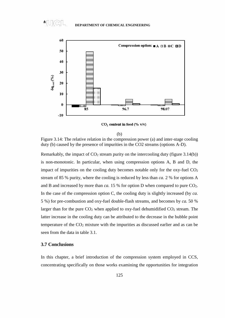
DEPARTMENT OF CHEMICAL ENGINEERING
125
(b)
Figure 3.14: The relative relation in the compression power (a) and inter-stage cooling
duty (b) caused by the presence of impurities in the CO2 streams (options A-D).
Remarkably, the impact of CO2 stream purity on the intercooling duty (figure 3.14(b))
is non-monotonic. In particular, when using compression options A, B and D, the
impact of impurities on the cooling duty becomes notable only for the oxy-fuel CO2
stream of 85 % purity, where the cooling is reduced by less than ca. 2 % for options A
and B and increased by more than ca. 15 % for option D when compared to pure CO2.
In the case of the compression option C, the cooling duty is slightly increased (by ca.
5 %) for pre-combustion and oxy-fuel double-flash streams, and becomes by ca. 50 %
larger than for the pure CO2 when applied to oxy-fuel dehumidified CO2 stream. The
latter increase in the cooling duty can be attributed to the decrease in the bubble point
temperature of the CO2 mixture with the impurities as discussed earlier and as can be
seen from the data in table 3.1.
3.7 Conclusions
In this chapter, a brief introduction of the compression system employed in CCS,
concentrating specifically on those works examining the opportunities for integration

DEPARTMENT OF CHEMICAL ENGINEERING
126
of the compression in CCS and the power generation process was presented. The
types of industrial compression technologies and the impurities present in the
captured CO2 streams were also discussed. This chapter further presented the
development and application of a detailed thermodynamic model to compute and
compare power requirements for various multistage compression strategies for CO2
streams. The CO2 streams considered included those captured from oxy-fuel and pre-
combustion coal-fired power plants. Several industrial compression options as
previously recommended for high-purity CO2 streams captured in a post-combustion
plant (Witkowski et al., 2013) were considered. The four compression options
examined included gas-phase compression using conventional multistage integrally
geared centrifugal compressors, supersonic shockwave compressors and multistage
compressors combined with subcritical as well as supercritical liquefaction and
pumping. In order to estimate the power demand for inter-stage cooling and
liquefaction, a thermodynamic model based on Carnot refrigeration cycle was applied.
Given the relatively high pressures of CO2 streams captured in oxy-fuel and pre-
combustion processes, the analysis was performed for the high-pressure compression
phase starting at 15 bar.
The results of a thermodynamic analysis performed for determining the power
requirements for the compression of CO2 streams for pipeline transportation and
subsequent geological sequestration were presented. It was found that for oxy-fuel
and pre-combustion CO2 streams of purity higher than ca. 96 % v/v, the compression
power for the four compression strategies examined was not significantly affected by
the presence of impurities. In case of the oxy-fuel stream with 85 % v/v CO2 purity,
the compression power requirement for the four compression schemes considered was
found to increase by ca. 12-30 % more than that for the compression of pure CO2.
Given that the power demand for compression increases with the amount of CO2
stream impurities which removal would raise the capture costs, there is a potential
trade-off between the costs of compression and purification. By combining the present

DEPARTMENT OF CHEMICAL ENGINEERING
127
methodology with a cost-benefit analysis model for the compression and purification,
an optimal CO2 stream purity for a given CCS plant may be determined.
The power demand for operating the inter-stage coolers is estimated to be relatively
small in comparison with the compression power demand (less than ca. 5 %) when
using the centrifugal and shock-wave compressors. However, when using
compression combined with subcritical and supercritical liquefaction and pumping,
the cooling system operation can take up about 50 % of the compression power when
applied to the oxy-fuel double-flash and pre-combustion CO2 streams. In the case of
oxy-fuel dehumidified CO2 mixture, the cooling power is predicted to be nearly 1.5
times higher than the compression power demand when applying to compression
combined with subcritical liquefaction and about 65 % of the compression power for
the compression combined with supercritical liquefaction and pumping.
The relatively high estimated power demand for the operation of the compressor
cooling system can be attributed to large cooling duties for the liquefaction of impure
CO2 streams. In particular, the cooling duty was shown to increase by up to 50 %
when compressing oxy-fuel CO2 with 85% v/v purity as compared to that for pure
CO2. Remarkably, for CO2 streams of higher than 96 % v/v purity, compression
combined with subcritical liquefaction and pumping can result in as much as ca. 15 %
increase in efficiency as compared to conventional centrifugal compression. The
liquefaction can be achieved at subcritical pressures around 62.53 bar using
conventional water cooling systems at temperatures in the range 10-20 oC. At the
same time, the study shows that operating such a system becomes less feasible for
lower grade CO2 streams due to incomplete liquefaction of the CO2 stream. In
particular, given the low bubble-point temperatures of oxy-fuel streams of ca. 85 %
CO2 purity, liquefaction at 62.53 bar would require using coolant temperatures as low
as -62 oC which would not be economically viable. This temperature may be
increased by applying CO2 liquefaction at higher pressures, however, to determine the

DEPARTMENT OF CHEMICAL ENGINEERING
128
optimal conditions for the liquefaction, the trade-off between the costs for operating
compressors and cooling/pumping system should be carefully considered.
In practice, a whole-system approach should be applied to optimise the compression
and purification system design and balance the costs associated with operation of
specific equipment, such as compressors and refrigeration units.

DEPARTMENT OF CHEMICAL ENGINEERING
129
CHAPTER 4:
TRANSIENT FLOW MODELLING IN CO2 PIPELINES DURING
LINE PACKING AND LINE DRAFTING
4.0 Introduction
During the pipeline transportation of CO2 in CCS operations, it is important to ensure
reliable and stable CO2 flow conditions at the injection point into the geological
storage site in order to ensure its efficient use and safe operation. However, flexible
operation (such as that encountered in the case of a fossil fuel power plant (section
4.1)) leads to a variable feed CO2 flow rate at the capture point and consequently
causing disturbances to the flow conditions in the transportation pipeline and
ultimately at the delivery point. In addition, given that the most economical mode of
pipeline transportation of CO2 is in the dense ‘liquid’ phase, unwanted two-phase flow
may occur in the event that the line pressure or temperature fall below the CO2
saturation conditions. This may result in cavitation or water-hammer effect with
associated mechanical vibration and pipe erosion and ultimately the real risk of pipe
failure (Liljemark et al., 2011).
As such, a properly designed and operated pipeline system is required in order to
maintain and allow the control of the CO2 flow rate, pressure and temperature in order
to avoid the above risks. ‘Pipe line packing’ is one of the most effective approaches
(Aghajani et al., 2017) with the pipeline acting as a battery to hedge against
intermittency. The term ‘line packing’ is generally used to describe the pipeline’s
buffering capacity where the pressure is varied to ‘pack’ more or less CO2 in the pipe,
which in essence, becomes a storage vessel. In pipeline terminology, increasing the
inventory (and hence the pressure) is called ‘line packing’, while decreasing it for
example during outflow or a drop in the feed flow rate is called ‘line drafting’. The
use of a pipeline as line packing is an appropriate control strategy to ensure that the

DEPARTMENT OF CHEMICAL ENGINEERING
130
fluctuation of the flow in the pipeline system may be minimised. For example, in
natural gas pipelines transmission, when the gas supply is interrupted, the line pack in
the pipeline starts drafting which continues to deliver gas to the downstream end.
In order to investigate the efficacy of line packing during line drafting method, an
appropriate mathematical model predicting transient fluid behaviour in the pipeline
system is required.
In the study by Chebouba (2015), the decision-making tool on the gas line pack
management of the “GZ1 Hassi R’mell-Arzew” gas pipeline was investigated by
applying NSGA-II mode FRONTIER solver in order to minimise the total power
consumption in the compression stations as well as to maximise gas line pack. From
the author’s study, a decision aid tool to make an appropriate decision for operators
can be provided to determine the discharge pressures and number of compressors to
be put in service. Aghajani et al. (2017) presented the results of the impact of pipeline
design and operation on the line packing capability by employing a statistical
analytical tool such as Artificial Neural Network (ANN) (Hagan et al., 1997). This
modelling software was shown to be a useful tool for evaluation of the available input
parameters to increase the capacity of the pipeline as line packing.
Currently, there are no reported detailed studies on assessing the hydraulic transient
analysis of line packing for CO2 pipelines. Given the markedly different fluid phase
behaviour of CO2 as compared to gaseous hydrocarbons such as natural gas, an
appropriate flow simulation tool is required to enable the transient analysis during line
packing and line drafting in CO2 transmission pipelines as part of their integration in
the CCS chain.
This chapter focuses on the development and testing of a numerical CFD model
developed for such purpose. The model is based on the numerical solution of the
conservation equations using the Method of Characteristics. It incorporates PR EOS
to deal with CO2 and its various mixtures. Following its verification, the numerical

DEPARTMENT OF CHEMICAL ENGINEERING
131
model is employed to conduct a systematic study on the impact of operational
flexibility involving a temporal reduction in the upstream CO2 feed flow rate on the
transient flow behaviour in the pipe over a period of 8 hours; typical for a fossil fuel
power plant during overnight operation. A particular focus of attention is determining
the optimum pipeline design and operating line packing conditions required in order
to maximise the delay in the transition from dense phase flow to the highly
undesirable two-phase flow following the ramping down of the CO2 feed flow rate.
The investigations are conducted for both pure CO2 and its various realistic mixtures
representative of the most common types of CO2 capture technologies.
As a means of its verification, in the case of transportation of CO2 in its dense phase,
(considered to be the most economical mode of its transportation), the numerical
model’s predictions are compared against those based on a simple analytical model
for incompressible flows.
4.1 Factors that influence the operating flexibility of power plants as part
of CCS
In order to achieve a carbon-neutral power supply for the future global energy system,
a significant increase in the proportion of renewable energy in the power supply mix
is required. To achieve this goal, the proportion of electricity generation from
renewable energy is expected to increase from 20 % in 2010 to 36 % in 2020, 44 % in
2030 and 52 % in 2050 (Capros et al., 2013). Hydro generation is the largest
contributor to renewable electricity in Europe but its potential is for the most part
already utilised.
This means that a significant part of the development of renewable electricity in the
future will be based on variable generation such as wind and solar photovoltaic.
However these energy supplies, like electricity demand, have a variable nature that is
not perfectly predictable. Consequently, short- and long-term variability and
uncertainty in the electricity load-generation balancing is likely to increase in the

DEPARTMENT OF CHEMICAL ENGINEERING
132
future. To cope with this increasing variability and uncertainty, the electricity system
will need to have sufficient flexibility to maintain the demand versus generation
balancing at all times (Hussy et al., 2014).
Flexibility is the ability of an electricity system to maintain continuous service in the
face of rapid and large fluctuations in supply or demand. Increasing amounts of
reserve power from firm sources of supply are needed as the total capacity of such
variable generators increases (Haines and Davison, 2009). Therefore, fossil-fired
power plants have to continue to play a significant role in ensuring the electric supply
balance demand. The majority of initial studies on CCS plant design and economics
have assumed that power plants installed with CCS will be ‘baseload’ plants, which
are very likely to be operated whenever they are available. Since many renewable
resources are intermittent, these fossil-fired power plants will, however, be expected
to be more responsive plants that will not always be used when they are available to
cope with this scenario (Chalmers et al., 2012).
As long as the share of variable Renewable Energy Sources (RES) in a power system
is low, the system can operate as usual. However, when RES is deployed on a large
scale, a new challenge emerges. This is precisely the situation that Europe is facing
today. When the wind stops blowing or the sun stops shining, gas-, coal-, and oil-fired
plants are employed to supply the needed electricity and to maintain the operational
requirements of the electrical grids. Sudden and massive requests for power, so-called
power ramps, create new requirements for conventional generators in the fossil-fired
power plant (Eurelectric, 2011).
The other factors that influence the operating flexibility of power plants are due to the
variable electricity demand. The value of electricity sales can also vary significantly
between jurisdictions and over time. For example, prices tend to be lower during the
night as demand is lower (Chalmers et al., 2009). Two possible scenarios which
follow variable electricity market demand trends are illustrated in figure 4.1
depending on the type of the plant itself.

DEPARTMENT OF CHEMICAL ENGINEERING
133
(a)
(b)
Figure 4.1: Pulverised Coal (PC) and Integrated Gasification Combined Cycle (IGCC)
(a) and Natural Gas Combine Cycle (NGCC) (b) plants operating load following
electricity demand trends (Domenichini et al., 2013).

DEPARTMENT OF CHEMICAL ENGINEERING
134
These include weekly (scenario 1) and daily (scenario 2) for different types of power
plants. In scenario 1, the PC, IGCC and NGCC plants are operated for 16 hours
during peak operation, while in the scenario 2; ca. 2 hours of electricity is demanded
during peak operation followed by 14 hours of normal operating conditions for all the
power plants employed as shown in figures 4.1(a) and (b).
In the case of off-peak operation during night time and weekends, PC and IGCC
plants are operated for 8 hours (figure 4.1(a)), whilst in the NGCC plant, the low
demand of electricity is utilised during this operation (figure 4-1(b)) (Domenichini et
al., 2013).
Employing the conventional fossil-fired power plants however will release both CO2
and atmospheric pollutants such as NOx, SO2 and particulate matters, which would
not be emitted by renewable energy sources (Eurelectric, 2011). While this is widely
recognised, the impact of part-loading during off-peak operation on the efficiency of
conventional thermal power plants is often neglected.
Even the most efficient fossil-fired power plant, Combined Cycle Gas Turbine
(CCGT)) will see efficiency drop significantly below its ‘normal’ efficiency when it is
not used at its rated full power. Such plants usually operate at an efficiency level of
about 55 % dropping to as low as 35 % when its load is reduced to 50 % or less of the
rated power output.
Part-loading of coal-fired plants and nuclear plants reduces efficiency by about
(maximum) 10 % (Eurelectric, 2011). The lower the efficiency, the smaller the power
produced for a given fuel input. However, the drop in efficiency increases the
quantities of CO2 and atmospheric pollutants produced per unit of electricity
generated. In other words, power plants emit more pollutants per kWh of electricity
produced than if operated at full capacity (Eurelectric, 2011).

DEPARTMENT OF CHEMICAL ENGINEERING
135
For these reasons, careful consideration should be given to retrofit the existing or new
fossil power plants with the Carbon Capture and Sequestration (CCS). In all CCS
schemes, CO2 is collected from a large point source before it is treated and
compressed for transport for safe geological sequestration (Chalmers et al., 2011).
4.1.1 Constant flow of CO2 to transport and storage
Most thermal power plants are designed for base load operation with a relatively
small number of starts and stops per year. The boundary conditions for thermal power
plants are thereby changing towards an increasing need for cyclic loads and operation
involving frequent starts and stops. In addition, the amount of CO2 produced by a
thermal power plant depends upon the electricity demand and its variation with time.
Demand can vary during the day as well as seasonally over the course of a year.
According to Jensen et al. (2016a), CO2 emissions are based on the load of the unit,
which can be fairly constant for 8-12 hours with only minimal change. At other times,
the load can change either higher or lower, at the rate of 1-2 % a minute. The 1 to 2 %
rate change can sometimes continue in the same direction for as long as 30-45
minutes. Because the changes are completely at the whim of the market, the operators
are not able to predict the load on an hour to hour basis. A CO2 capture plant
associated with an electricity-generating station will be forced to adapt to this type of
variation in both quantity of CO2 produced and in the flue gas composition with time.
The requirement of the power plants to follow a variable electricity market demand
trend leads to an uneven captured CO2 flow rate and a consequent fluctuation of the
operating conditions in the pipeline and sequestration site. In addition, in practice, it is
important to understand the impact of variable CO2 loading on the flow behaviour in
the associated pipeline system. Based on the study by Liljemark et al. (2011) on the
effect of a load change in the pipeline it was found to result in the slow formation of
two-phase flow in the pipe. According to the study by Klinkby et al. (2011) during
shut-down process, the pressure and temperature dropped below the critical point and

DEPARTMENT OF CHEMICAL ENGINEERING
136
phase changed from dense phase to gas and liquid were occurred in the upper part of
the well and in the pipeline. Using very low loads of less than 20 % of the full load
will cause problems with keeping the supercritical conditions along the pipeline and
in the well due to a combination of lower pressure and cooling.
As a consequence, a properly designed preventive measure is required to maintain a
constant CO2 flow rate in the pipeline system, thus avoiding pressure fluctuations and
consequent possible changes of the CO2 physical state. Such a measure is the focus of
the present study, discussed in the next section.
4.1.1.1 Pipeline packing
A CO2 pipeline system can be controlled so that the supply and demand of CO2 can be
regulated. The introduction of strategically placed temporary storage into pipeline
system can help to attenuate variation. There are different types of temporary storage
including pipeline packing, where the storage can be achieved by increasing the gas
pressure and loading more gas into a pipeline. In response to the upset operation
conditions, use of a pipeline line pack across the consolidated network of pipelines
and storage facilities can be used like a battery to hedge against intermittency. A line
pack depends on the pressure levels in the pipeline, and it constantly changes as
pressure is varied. Typically, pipelines build up line pack during periods of decreased
demand and draw it down during periods of increased demand (Rigos et al., 2011).
To illustrate a line packing scenario, a simple pipeline system with a compressor
station and a mainline valve at the end of the pipeline is shown in figure 4.2. The
pipeline has been operating in steady state condition for a long time as indicated by
the solid line in figure 4.2.

DEPARTMENT OF CHEMICAL ENGINEERING
137
Figure 4.2: Pipeline packing (Menon, 2005).
During line packing, the flow of fluid out of the pipeline is stopped by closing (or
throttling) a downstream valve whilst still allowing fluid to flow into the pipeline
upstream. As a result, the fluid contained in the pipeline is compressed (packed) and
the pressure of the contained fluid within the pipeline increases as shown by the
dashed lines in figure 4.2. This will result in an increase in line pack in the
downstream section of the pipe, which will progress toward the upstream end. The
transient pressure waves moving upstream will eventually reach the discharge of the
compressor, causing the discharge pressure to rise. If the increased pressure attains the
Maximum Allowable Operating Pressure (MAOP) of the pipeline, the downstream
valve will open.
A line pack is highly dependent on pipeline specifics. In the case of a natural gas
system, depending on the length of the supply chain, it takes many hours or even days
for natural gas to complete the journey from the wellhead to the city-gate in order to
replenish the line-pack. Communication between the Independent System Operator
(ISO) and the pipeline about mass flow variability could enable a pipeline to increase
a line pack before an interruption in flow event. Even better, routine operating
procedures should be developed to ensure pipeline readiness to supply fluid in
response to an abrupt reduction in the flow rate. A pipeline and the suppliers behind it
must be compensated for the additional fuel used to replenish the line pack in order to

DEPARTMENT OF CHEMICAL ENGINEERING
138
offset under-performance when the mass flow is lower than expected (Rigos et al.,
2011).
Aghajani et al. (2017) investigated the impact of pipeline design and operation on the
line packing capability of a dense phase CO2 pipeline network. The results produced
are illustrated in figure 4.3 showing the effect of varying pipeline length, mass flow
rate and inlet as well as outlet pressure on line packing time for a fixed inner diameter
of the pipeline transporting pure dense phase CO2.
Figure 4.3: Effect of changes in flow rate and inlet and outlet pressure management
on the line-packing time for a 457 mm outer diameter, 11 mm wall thickness pipeline
containing pure dense phase CO2 (Aghajani et al., 2017).
According to the data presented, the biggest effect of changing the pressure at the
inlet and outlet was observed at lower flow rates. At the lower flow rates, changing
the outlet pressure condition increases the line packing time by approximately 70 %
for all pipeline lengths. From the results, the authors claimed that if a combined
strategy of managing the outlet pressure and lowering the flow rate is possible, then

DEPARTMENT OF CHEMICAL ENGINEERING
139
the line packing times can be increased by factors of up to five times depending on
pipeline length.
4.1.1.2 Pipeline drafting
Much of the short-term (i.e. daily and hourly) gas demand variation is accommodated
by drawing from aboveground liquefied gas storage vessels or by an intentionally
varying pipeline operation by increasing and decreasing pressure so as to use the
pipeline for temporary storage. The practice, termed “line packing” or “packing,”
increases the volume stored while “drafting” or “de-packing” reduces the volume
(Jensen et al., 2016a). When the gas supply is interrupted, the line pack in the pipeline
starts reducing which continues to deliver gas to the downstream end. During this
scenario, the pressures continue to fall along the pipeline for a certain period of time
(Menon, 2005).
Currently there is no methodology for assessing the line drafting characteristics of
dense phase CO2 pipelines.
The following presents the development of a numerical transient pipe flow model for
simulating line packing and line drafting in pressurised CO2 pipelines. This then
followed by its application to realistic case studies to test its efficacy as a tool for
investigating line packing as a means for smoothing out flow transients following a
disturbance in the upstream pipe flow conditions and the subsequent impact on the
fluid phase during line drafting.
4.2 Numerical pipe flow model
4.2.1 Governing equations
In this study, the multiphase transient pipe flow is approximated by the Homogeneous
Equilibrium Mixture (HEM) model where the constituent phases are assumed to
remain at thermal and mechanical equilibrium during decompression. The

DEPARTMENT OF CHEMICAL ENGINEERING
140
corresponding conservation equations expressed in terms of pressure, P, specific
entropy, s and flow velocity, v as dependent variables are given by:
02
x
va
dt
ds
dt
dP 4.1
sin2
gvvD
f
x
P
x
vv
t
v w
4.2
D
vfq
dt
dsT w
h2
3 4.3
where θ, g, ρ, T, a and D are respectively the pipeline elevation, gravitational
constant, density, temperature, speed of sound and pipe inner diameter, a function of
time, t and space, x while is given by the thermodynamic function,
s
Pand fw is
the Fanning friction factor calculated using Chen’s correlation as described in sections
2.4.5.2 and 2.4.6, respectively. hq is the heat flux at the pipe wall and is defined via
the heat transfer equation as described in section 2.4.5.4.
4.2.2 Boundary conditions
The conservation equations presented in the equations 4.1-4.3 are closed by the
boundary conditions as presented in the following section.
4.2.2.1 Variable flow rate at the pipeline inlet
In this study, to account for the variation of the flow rate at the pipe inlet, the local
conservation equations are first modified following Thompson (1987) and Thompson
(1990), which read:
02
111322
at
4.4
02
113
t
P 4.5
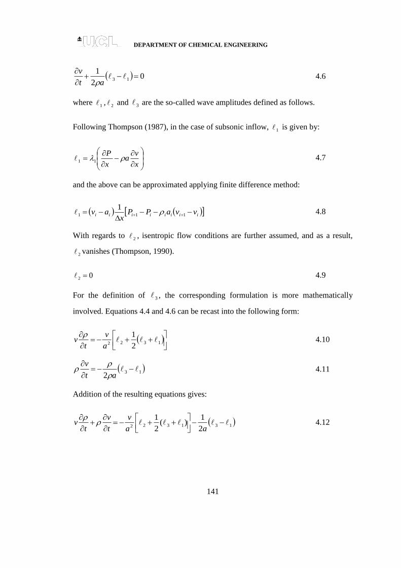
DEPARTMENT OF CHEMICAL ENGINEERING
141
02
113
at
v
4.6
where 1 ,
2 and 3 are the so-called wave amplitudes defined as follows.
Following Thompson (1987), in the case of subsonic inflow, 1 is given by:
x
va
x
P11 4.7
and the above can be approximated applying finite difference method:
iiiiiiii vvaPPx
av
111
1 4.8
With regards to 2 , isentropic flow conditions are further assumed, and as a result,
2 vanishes (Thompson, 1990).
02 4.9
For the definition of 3 , the corresponding formulation is more mathematically
involved. Equations 4.4 and 4.6 can be recast into the following form:
1322 2
1
a
v
tv
4.10
132
at
v
4.11
Addition of the resulting equations gives:
131322 2
1)(
2
1
aa
v
t
v
tv
4.12

DEPARTMENT OF CHEMICAL ENGINEERING
142
Note the RHS of equation 4.12 is simply the expanded form of the rate of change in
the flow rate, t
v
. Knowing
1 and 2 (see equations 4.8 and 4.9), 3 can now be
expressed in terms of t
v
, such that:
ii
iiii
av
avAav
1
2
23
22 4.13
where:
vt
A
4.14
Herein, A is specified based on specific requirements by operational flexibility (see
section 4.1).
In the present study, the calculation of mass flux, v over the time during the ramping
down process is introduced by the following hyperbolic tangent function:
xv tanh 4.15
where the coefficients of , and x respectively represent the reduction trends of the
mass flux during ramping down, while the relationship of and can be fitted in the
form of ov . Here ov represents the mass flux at the initial conditions.
In order to determine the specific requirements of the ramping down during flexible
operation following the reduction of the mass flux to 50 % of its initial value, the
extension of the equation 4.15 as a function of time can be expressed as:
28800t1700 if 5.0
1700t1000 if 4100
1000tanh
4
1000t0 if
o
oo
o
o
v
vv
tv
v
v
4.16

DEPARTMENT OF CHEMICAL ENGINEERING
143
Here the value of A (see equation 4.14) can be determined from the derivation of the
relative function of equation 4.16:
28800t1700 if 0
1700t1000 if 100
1000sec
1004
1000t0 if 0
2 th
vv
t
o 4.17
Along with equation 4.17, it is therefore possible to predict the variable mass flux for
that particular time. In the case study, the valve closure is set to be started at 1000 s
within 700 s. After this period, the value of mass flux is set constant to 50 % of its
initial value within 28800 s (8 hours) of operation. It is highlighted that the
relationships developed in equations 4.15-4.17 are only applicable to the modelled
case studies.
To this end, the local governing equations at the pipe inlet are readily solved.
Applying backward Euler method, the corresponding primitive variables flow
velocity, v and pressure, P are given by:
j
jj
jjjj
j ua
tavavv
2
13
12
4.18
j
j
jjjj
j Pta
avavP
3
13
12
4.19
where, j represents the known values at the previous time level and 1j is the
unknown values at the current time level. As entropy is assumed constant for inflow,
other pertinent fluid properties can be calculated by performing the pressure-entropy
flash calculations, using Peng-Robinson Equation of State (PR EOS), previously
presented in section 2.1.6.

DEPARTMENT OF CHEMICAL ENGINEERING
144
4.2.2.2 Outlet boundary condition
At the outlet of the pipeline, simple zero-order extrapolation method is applied, where
all variables are equated to the corresponding values at the last numerical cell centre
in the computational domain.
4.2.3 Numerical method
Using MOC (see section 2.4.7.1), the conservation equations 4.1 to 4.3 may be
replaced with three compatibility equations along their corresponding characteristic
lines by:
tdT
sd oo
4.20
along the Path line characteristic ( oC ):
vxd
td 1
0
0 4.21
tdT
avadPd t
4.22
along the positive Mach line characteristic ( C ):
avxd
td
1 4.23
tdT
aPdvad
4.24
along the negative Mach line characteristic ( C ):
avxd
td
1 4.25
The values of P, s, ρ, v and a , as a function of time and distance along the pipeline
are obtained by the inverse marching method of characteristics as described in chapter

DEPARTMENT OF CHEMICAL ENGINEERING
145
2. This involves dividing the pipeline into a large number of distance (Δx) and time
elements (Δt) and expressing the compatibility equations in finite difference form
paying due regard to the Courant stability criterion (equation 2.114) regarding the
maximum allowable distance and time elements. These finite difference equations are
in turn solved at the intersection of the linear characteristics lines with the spatial axis
using iteration and interpolation in conjunction with P-s (pressure-entropy) flash
calculations.
4.3 Analytical model
As explained earlier (see section 4.3), despite its rigour, the numerical transient pipe
flow model described above is computationally demanding. In practice, this restricts
its use for routine applications. In an attempt to address this shortcoming, and for its
verification, the following describes the development of a simple analytical pipe flow
model based on the assumption of incompressible and isothermal flow where all the
fluid in the pipe travels at the same velocity. This is a reasonable approach given that
as mentioned previously, the most economical method for transportation of CO2 is in
the dense phase (Chaczykowski and Osiadacz, 2012, Witkowski and Majkut, 2012)
where the liquid like fluid will have a small compressibility. The above is then
followed by testing of the analytical model’s applicability based on the comparison of
its predictions against those obtained from the numerical pipe flow model.
The resulting momentum conservation for incompressible isothermal flow reads
(Apsley, 2013):
sin2
gvvD
f
L
P
dt
dv w
4.26
where v, L and D are respectively the velocity, pipeline length and inner diameter of
the pipe, while ΔP is the pressure drop across the length of the pipe. The latter is
obtained from the predictions from the numerical flow model presented in section 4.3.

DEPARTMENT OF CHEMICAL ENGINEERING
146
To solve the above equation 4.26, the differential-algebraic solver library DASSL
(Brenan et al., 1996) is employed. The thermodynamic properties of CO2 are
determined using the Peng-Robinson Equation of State (section 2.1.6).
4.4 Results and discussion
In this section, the simulation results are divided into three parts. In the first part,
simulations of the unsteady impure CO2 flow in response to a change in the upstream
CO2 feed flow rate (e.g. from the power plant) are performed to investigate the impact
of load fluctuation on the transported fluid in the pipe. Also included in the same
section is a case study investigating the influence of the line packing on maintaining
the near-steady flow condition for pure dense phase CO2 during flexible operation.
The tests are performed include employing both the simple analytical and the
computationally demanding numerical pipeline flow model for verification purposes.
In the second part, the optimum pipeline design and operation parameters including
pipeline dimensions, inlet temperature as well as inlet mass flow rate for the line
packing method are determined. Finally, the efficacy of the optimised variables for
the design stage of line packing is tested for the CO2 streams containing various types
of stream impurities.
4.4.1 Effect of operational flexibility on pipeline flow
In order to study the effect of operational flexibility on the pipe flow in the context of
CCS, a case study is carried out applying pipeline flow models developed above.
Table 4.2 shows the pipeline dimensions, and the prevailing conditions for the case
study.

DEPARTMENT OF CHEMICAL ENGINEERING
147
Table 4.2: Simulation input data for the case study.
Parameter Value
Initial pressure (bar) 150
Initial temperature (K) 311.15
Ambient temperature (K) 278.15
Ambient pressure (bar) 1.01
Pipeline length (km) 50
Pipeline thickness (mm) 10
Pipeline outer diameter (mm) 457
Fanning friction factor 0.002
Pipe roughness (mm) 0.0457
Number of grids 2000
Pipe orientation to the horizontal plane (o) 0
Feed flow rate (kg/s) 100
Heat transfer coefficient (W/m2K) 5
Material of construction Stainless steel
CFL factor 0.9
Feed CO2 composition (% v/v):
Pure CO2
Pre-combustion
Oxy-fuel:
Double flashing
100
98.07
96.7
Raw/dehumidified 85
The test case relates to a 50 km length, 457 mm outer diameter and 10 mm wall
thickness horizontal steel pipeline transporting CO2 and its various mixtures
corresponding to pre-combustion and oxy-fuel capture technologies. The feed
compositions in the CO2 streams employed are presented in table 3.1. Given the
relatively small proportion of impurities, post-combustion CO2 stream (see table 3.1),
is not considered in the study. The feed flow rate is assumed to be 100 kg/s at 150 bar
and 311.15 K. Under these conditions, the CO2 streams are in the supercritical state.
The pipe roughness assumed to be 0.0457 mm corresponding to mild steel (McCoy
and Rubin, ). The simulation is performed using a computational grid of 2000
equally-spaced numerical cells with a CFL factor of 0.9.
In order to simulate a flow disturbance for example, as a result of a change in loading
or due to a gradual feed valve closure, at 1000 s the pipe feed flow rate is assumed to

DEPARTMENT OF CHEMICAL ENGINEERING
148
decrease to 50 % of its initial value over a period of 700 s in a non-linear manner
following the function given by equation 4.17 (section 4.3.2.1).
Figures 4.4 and 4.5 respectively show the corresponding simulated fluid velocity,
pressure, temperature and density variations with time at the pipeline inlet and outlet
over 16650 s of simulation time. All data were generated using the transient numerical
pipe flow model. The vertical dashed, dotted and solid lines for all the mixtures as
shown in figure 4.4(a) mark the start (1000 s) and the completion (1700 s) of the feed
flow ramp down.
As it may be observed in figure 4.4(a), for all CO2 concentrations considered, the
commencement of valve closure at 1000 s is marked by a rapid and almost of
instantenous drop in the flow velocity to constant values throughout the rest of the
simulation time.

DEPARTMENT OF CHEMICAL ENGINEERING
149
(a) (b)
(c) (d)
Figure 4.4: The transient variations in velocity (a), pressure (b), temperature (c) and density (d) for pure CO2 and CO2 with impurities at
pipeline inlet following the linear ramping down of feed flow rate. The vertical dotted lines indicate mark the start (1000 s) and the
completion (1700 s) of the feed flow ramp down at a rate of 100 kg/s down to 50 % of the initial value. Inlet pressure = 150 bar, inlet
temperature = 311.15 K, mass flow rate = 100 kg/s, pipe length = 50 km and inner pipe diameter = 437 mm (see also table 4.2).

DEPARTMENT OF CHEMICAL ENGINEERING
150
(a) (b)
(c) (d)
Figure 4.5: The transient variations in velocity (a), pressure (b), temperature (c) and density (d) for pure CO2 and CO2 with impurities at
pipeline outlet following the linear ramping down of feed flow rate. The vertical dotted lines indicate mark the start (1000 s) and the
completion (1700 s) of the feed flow ramp down at a rate of 100 kg/s down to 50 % of the initial value. Inlet pressure = 150 bar, inlet
temperature = 311.15 K, mass flow rate = 100 kg/s, pipe length = 50 km and inner diameter = 437 mm (see also table 4.2).
DEPARTMENT OF CHEMICAL ENGINEERING
151
As compared to the fluid velocity, the fluid pressure (figure 4.4(b)) and temperature
(figure 4.4(c)) also show a drop in their magnitudes at 1000 s, but this is followed by
a much lower rate of decrease remaining relatively constant in the first 13300 s. This
is followed by a second inflection in the slope as indicated by the vertical dashed
lines, marking the transition from the supercritical to the two-phase state (see latter in
figure 4.7). The observed drop in the fluid temperature throughout is due to its
depressurisation induced expansion cooling.
In contrast, the commencement of valve closure is not marked by a noticeable
discontinuity in the fluid density (figure 4.4(d)), where a much lower rate of drop as
compared to the fluid pressure, velocity and temperature is observed.
Turning to the effect of CO2 stream impurities on the flow transients resulting from
the partial inlet valve closure as shown in figures 4.4 and 4.5, it is clear that all the
flow parameters are affected by the presence of impurities, with the impact increasing
with the percentage of the impurity. The raw-dehumidified oxy-fuel mixture with 85
% v/v CO2 shows the highest reduction in flow parameters compared to other streams.
In the case of pre-combustion (98.07 % v/v CO2) and double flashing oxy-fuel
mixture (96.7 % v/v CO2), the flow parameters are almost the same as with pure CO2.
Returning to the data in figure 4.5 showing the corresponding transient variations in
the flow parameters at the pipe outlet following the disturbance in the feed flow rate.
As it may be observed, in contrast to the behaviour at the pipeline inlet (figure 4.4),
the commencement of the closure of the inlet valve is not marked by the nearly
instantaneous rapid drop in the flow velocity (figure 4.5(a)) at the pipe outlet. Apart
from this, and with exception of marginal drops in their values, all the trends
observed, including those for the various CO2 impurity streams, are very similar to
those at the pipe inlet. The vertical dashed lines mark the transition from the
supercritical to the two-phase state.

DEPARTMENT OF CHEMICAL ENGINEERING
152
To aid clarity, figure 4.6 shows the superimposed plots of the transient variations of
the flow parameters at the pipe inlet and outlet plotted for the pure CO2 chosen as an
example.
As it may be observed, in the case of the fluid temperature, pressure and density, the
deviation between the inlet and outlet values occurs at approximately 13300 s
following the start of valve closure.

DEPARTMENT OF CHEMICAL ENGINEERING
153
(a) (b)
(c) (d)
Figure 4.6: The transient variations in velocity (a), pressure (b), temperature (c) and density (d) for pure CO2 at pipeline inlet and outlet
following the linear ramping down of feed flow rate. The vertical dotted lines indicate mark the start (1000 s) and the completion (1700
s) of the feed flow ramp down at a rate of 100 kg/s down to 50 % of the initial value. Inlet pressure = 150 bar, inlet temperature = 311.15
K, inlet mass flow = 100 kg/s, pipe length = 50 km and inner diameter = 437 mm (see also table 4.2).

DEPARTMENT OF CHEMICAL ENGINEERING
154
As mentioned above, the second inflections observed in the slopes of the curves
indicated in figures 4.4-4.6 occuring after ca.13300 s correspond to the change in the
fluid phase from supercritical to the two-phase state. To illustrate this further, figure
4.7 shows the fluid phase diagrams presented in the form of dew point and bubble
point curves for pure CO2 and the three CO2 mixtures under consideration. This data
was generated using the REFPROP (Lemmon and Huber, 2010) physical properties
model incorporating the PR EOS.
Also included in each plot are the corresponding pressure and temperature trajectories
at the pipe inlet and outlet during valve closure as extracted from figures 4.4(b-c) and
4.5(b-c). As it may be observed, for the most part, the fluid within the pipeline
remains in the supercritical state. Given the very high speed of sound in the
supercritical state (ca. 1000 m/s; (Han et al., 2010)), this explains the marginal
diffrence in the fluid properties at the pipe inlet and outlet at any given time during
the feed ramping down (see figure 4.7).
The intersection of the pressure/temperature trajectories with the bubble point curves
marks the transition from the supercritical to the two-phase state. This is in turn
manifested in the second inflections in the rate of change in the fluid properties as
shown in figures 4.4 to 4.6 occuring at 13300 s where the deviations between the fluid
parameters becomes more pronounced due to the lower speed of sound (ca. 350 m/s;
Han et al., 2010) in the two-phase mixtures.

DEPARTMENT OF CHEMICAL ENGINEERING
155
(a) (b)
(c) (d)
Figure 4.7: Pipe inlet and outlet pressure-temperature trajectories in relation to the dew and bubble point curves following the non-linear
ramping down of feed flow rate for pure CO2 (a), double flashing (b), pre-combustion (c) and raw/dehumidified (d) compositions.

DEPARTMENT OF CHEMICAL ENGINEERING
156
Table 4.3 lists the temperatures and pressures at which the transition from the
supercritical to the two-phase region occurs for the pure CO2 and its various mixtures.
As it may be observed the pressure at which the transition to the two-phase state
occurs increases with the decrease in the purity of the CO2 stream.
Table 4.3: The supercritical to two-phase transition pressures and temperatures as a
function of CO2 purity (see table 3.1 for mixture compositions).
% v/v CO2 Transition pressure
(bar)
Transition
temperature (K)
Pure CO2 100.0 58 293.8
Pre-combustion
Oxy-fuel:
98.07 73.1 295.5
Double flashing 96.7 69.2 293.9
Raw/dehumidified 85.00 94.7 292.1
In practice the above means that as the proportion of impurities incerases in the CO2
stream, higher operating line pressures are required in order to avoid the risk of the
undesired two-phase flow occuring during feed ramping down process. In the case of
the raw/dehumidified CO2 mixture for example, the line pressure must not fall below
94.7 bar and exceed 292.1 K at any time to ensure operation in the dense phase.
In order to compensate for such upset condition as well as to maintain the operating
pressure above the critical point, utilising the pipeline as line packing will be
considered in section 4.5.2.
4.4.1.1 Performance of the analytical model
As the chosen conditions of the CO2 stream during valve closure following flexible
operation is ‘nearly incompressible’ (the fluid stays in the dense phase supercritical
state during the most part), the predictions from the simplified analytical
incompressible flow model describe in section 4.4 is compared against those obtained
from the computationally demanding numerical pipeline model. The transmission
pipeline is assumed to be 50 km long, outer diameter of 400 mm and 20 mm wall
thickness transporting pure CO2 at feed temperature and pressure of 293.15 K and 95

DEPARTMENT OF CHEMICAL ENGINEERING
157
bar respectively. The remaining pertinent flow, ambient and computational
parameters are set the same as those given in table 4.2.
Figure 4.8 shows a comparison of the predicted fluid velocity profiles as a function of
time at both ends of the test pipe predicted from both models. Expectedly, the
analytical model is presented only by a curve given that it is based on incompressible
flow assumption. On the other hand, in the case of pipeline flow model, two
distinctive velocity profiles are predicted; those at the pipeline inlet and outlet.
Figure 4.8: Comparison of time variation of the fluid flow velocity based on the
numerical (solid and square dot lines) and analytical pipe flow models (rounded
dotted line).
It is interesting to note that the fluid velocity transient predicted using the analytical
model lies mostly in between the inlet and outlet velocities produced from the
numerical pipeline flow model. In particular, the velocity profiles calculated from the
numerical model predicts the velocity stabilisation after ca.700 s.

DEPARTMENT OF CHEMICAL ENGINEERING
158
4.4.2 Optimal parameter investigation for avoiding two-phase flow during
flexible operation
The following presents the results of a series of parametric investigations determining
the impact of the various design and operation parameters on the time taken for the
transition from supercritical to the undesired two-phase flow at the delivery point
following the ramping down of the supercritical CO2 feed flow rate. The above
mimics’ the flexible operation of a coal power plant, for example during night-time
power ramp down. Such information is highly useful in practice from an operational
point of view.
The parameters investigated include pipeline diameter, length, inlet temperature and
mass flow rate. The simulations are performed using the numerical model, based on
ramping down of the feed flow rate after 1000 s of steady flow operation by 50 %
over 700 s following the ramping down function given by equation 4.17. Unless
otherwise stated all the conditions tested are the same as those given in table 4.2.
4.4.2.1 Effect of pipeline dimension
Three pipeline lengths of 50 km, 100 km and 150 km corresponding to the pipe inner
diameters and wall thicknesses presented in table 4.4 are investigated.
Table 4.4: Pipeline dimensions.
Inner diameter (mm) Wall thickness (mm)
437 10
486 11
535 12
584 13
874 20
The pipe thicknesses presented in table 4.4 are the minimum safe design values
calculated using equation 4.27 (McCoy and Rubin, 2008) based on the maximum
operating pressure of 150 bar.

DEPARTMENT OF CHEMICAL ENGINEERING
159
SEF
DPThickness oMOP
2 4.27
where PMOP, Do, S, E and F are the maximum operating pressure of the pipeline, the
outer pipe diameter, the specified minimum yield stress for the pipe material, the
longitudinal joint factor and the design factor, respectively. In order to determine the
thickness of the pipe, the longitudinal joint factor is set to 1.0, the design factor is 0.72
and the minimum yield stress is 4830 bar for mild steel (McCoy and Rubin, ).
Figure 4.9 shows the simulated variation of line drafting time (defined as the time
lapsed to reach the two-phase flow) at the pipe end for various pipeline lengths and
inner diameters following the commencement of feed ramp down to 50 % of its initial
value for pure CO2.
Figure 4.9: Effect of pipeline dimensions on the line drafting time for pure CO2
following feed ramp down. Parameters: inlet pressure = 150 bar, inlet temperature =
311.15 K, ambient temperature = 278.15 K, inlet mass flow = 100 kg/s and pipe
thickness (see table 4.4).
As can be seen in figure 4.9, the line drafting time is significantly affected by the
length and the inner diameter of the pipeline. For the same pipeline length, the line
drafting time (the time lapsed to reach the two-phase flow) increases with an increase

DEPARTMENT OF CHEMICAL ENGINEERING
160
in the pipe inner diameter, with the effect decreasing with increase in the pipeline
length. For the maximum pipeline length of 150 km, in the ranges tested, the increase
in the pipe inner diameter beyond 486 mm has no impact on the line drafting time.
On the other hand, for the same pipe inner diameter, the line drafting time generally
increases with the pipe length. In the case of the 150 km pipeline however, no further
increase in the line drafting time may be observed beyond a pipe internal diameter of
486 mm.
The precise mechanism-giving rise to the above observed trends is difficult to discern.
The most likely explanation is that these arise because of counteracting interaction of
pipeline length and diameter. The reduction in the pressure drop with increase in pipe
diameter results in a delay in the transition to two-phase flow and hence an increase in
the line drafting time. On the other hand, an increase in the pipeline length results in
an increase in the pressure drop resulting in an increase in the line drafting time.
According to the data in figure 4.9, the shortest length of the pipe (50 km) with the
largest inner diameter (874 mm) just satisfies the single phase flow condition for 8
hours (28800 s) of operation; typical duration for the ramping down of a power plant
during night-time operation. For this reason, preserving the practical context, the
proceeding investigations are performed based on these pipeline dimensions.
4.4.2.2 Effect of feed stream inlet temperature
To elucidate the effect of feed stream inlet temperature on the line drafting time, the
inlet temperature in the 50 km pipeline with 874 mm inner diameter is assumed to
vary from 283.15 to 311.15 K. The corresponding data for pure CO2 are shown in
figure 4.10.

DEPARTMENT OF CHEMICAL ENGINEERING
161
Figure 4.10: Effect of feed temperature on the line drafting time for pure CO2.
Parameters: inlet pressure = 150 bar, ambient temperature = 278.15 K, inlet mass flow
= 100 kg/s, pipeline length = 50 km and pipeline inner diameter = 874 mm.
As it may be observed from figure 4.10, the line drafting time increases almost in a
linear manner with increasing feed temperature up to 303.15 K, beyond which no
further increase in the line drafting time is obtained. The increase in the feed
temperature results in two counteracting factors affecting the line drafting time:
i) reduction in the viscosity of dense phase CO2 (Moshfeghian, 2009), leading to
a reduction in the pressure drop and hence an increase in the line drafting time.
ii) the lowering of the pressure at which two-phase flow occurs thus resulting in
a decrease in the line drafting time.
Based on the data presented in figure 4.10, it is reasonable to postulate that the effect
of the reduction in viscosity is the dominant factor up to the feed temperature of
311.15 K. Beyond this temperature, this effect is counteracted by the earlier transition
to two-phase flow with the net effect of only a marginal increase in the line drafting
time. In keeping with a practical perspective, given that a high feed temperature poses

DEPARTMENT OF CHEMICAL ENGINEERING
162
the risk of damage to the pipeline external coating (Chaczykowski et al., 2012), an
inlet temperature of 303.15 K is chosen for the proceeding investigation.
4.4.2.3 Effect of feed mass flow rate
Figure 4.11 shows the variation of line drafting time against initial CO2 feed mass
flow rate in the range of 100 to 150 kg/s for 874 mm inner diameter, 50 km long pipe.
As it may be observed, the increase on the mass flow rate and hence the increase in
the pressure drop results in a drop in the line drafting time from a maximum value of
28800 s (100 kg/s feed) to 23707 s (150 kg/s feed).
Figure 4.11: Effect of initial feed mass flow rate on the line drafting time of pure CO2.
Parameters: inlet pressure = 150 bar, inlet temperature = 303.15 K, ambient
temperature = 278.15 K, pipeline length = 50 km, pipeline inner diameter = 874 mm.
Also an initial feed flow rate of 100 kg/s can maintain the dense phase in the pipe for
8 hours following the feed ramp down.
4.4.3 Application of the optimised line packing parameters
The following presents the results of a case study demonstrating the efficacy of the
flow model presented above (see section 4.3) as a design and operational control tool

DEPARTMENT OF CHEMICAL ENGINEERING
163
for avoiding two-phase flow for CO2 pipelines following feed ramping and line
drafting. Figures 4.12 and 4.13 respectively show the variation of pressure and
temperature as a function of time at the pipeline inlet and outlet for a 50 km, 874 mm
inner diameter pipeline containing CO2 and its various mixtures based on the various
capture technologies. The data are presented over 8 hours duration (28800 s)
representing the overnight flexible operation of a power plant. The feed flow rate is
assumed to be gradually ramped down from maximum of 100 kg/s to 50 kg/s over
700 s following the control function given by equation 4.17. All the remaining
relevant parameters are given in the figure caption and table 4.4.
(a)
(b)
Figure 4.12: Change in pressure (a) and temperature (b) of pure CO2 and CO2 with
impurities at pipeline inlet during flexible operation. Parameters: inlet pressure = 150
bar, mass flow rate = 100 kg/s, inlet temperature = 303.15 K, ambient temperature =
278.15 K, pipeline length = 50 km and pipeline inner diameter = 874 mm.

DEPARTMENT OF CHEMICAL ENGINEERING
164
(a)
(b)
Figure 4.13: Change in pressure (a) and temperature (b) of pure CO2 and CO2 with
impurities at pipeline outlet during flexible operation. Parameters: inlet pressure =
150 bar, mass flow rate = 100 kg/s, inlet temperature = 303.15 K, ambient
temperature = 278.15 K, pipeline length = 50 km and pipeline inner diameter = 874
mm.
Figure 4.14 shows the variation of the pressure and temperature trajectories as
extracted from the data in figures 4.12 and 4.13 for the pure CO2 and its three
mixtures superimposed on the corresponding vapour liquid equilibrium diagrams. As
it is clear, none of the pressure/temperature trajectories cross the two-phase envelope.
This means that for the design and operational conditions chosen, the CO2 stream and
its mixtures will remain in the supercritical dense phase during the overnight power
ramping down process.

DEPARTMENT OF CHEMICAL ENGINEERING
165
(a) (b)
(c) (d)
Figure 4.14: Pressure-temperature diagram of pure CO2 (a), double flashing (b), pre-combustion (c) and raw/dehumidified (d) showing the fluid
flows in supercritical condition during flexible operation. Parameters: inlet pressure = 150 bar, mass flow rate = 100 kg/s, inlet temperature =
303.15 K, ambient temperature = 278.15 K, pipeline length = 50 km, pipeline inner diameter = 874 mm.

DEPARTMENT OF CHEMICAL ENGINEERING
166
CHAPTER 5:
CONCLUSIONS AND RECOMMENDATIONS FOR FUTURE
WORK
5.1 Conclusions
This thesis described the development and testing of rigorous mathematical models
for
i) determining the power consumption for multistage compression with
intercooling for transporting high pressure CO2 and the optimum
configurations for such systems
ii) simulating the transient flow in high pressure CO2 pipelines with line packing
and line drafting during flexible operation
The following is a summary of the main findings.
In chapter 2, the basic thermodynamic and energy balance relations for calculating the
power requirement of multistage compression and cooling duty were discussed. These
presented equations coupled with a cubic equation of state representing the foundation
of the multistage compression model. The thermodynamic relations for predicting the
pertinent fluid properties such as the fluid enthalpy, entropy and discharge
temperature were also presented.
The application of the general equations for modelling multistage compressor and
intercooler for the CO2 pipeline transportation was reviewed. Most of the reviewed
studies have focused on design and optimisation of compression systems capable of
handling the operating constraints for near pure CO2 streams as well as examining the
opportunities for integration of the compression in CCS and the power generation
process. Practically, the CO2 streams in CCS will contain some impurities, whose
nature and concentrations depend on the emission source and capture technology

DEPARTMENT OF CHEMICAL ENGINEERING
167
applied. In this thesis, the effect of CO2 impurities from various capture technologies
on the power requirement of several industrial compression schemes as those
previously recommended for near pure CO2 streams captured in a post-combustion
plant were investigated.
In the second part of chapter 2, the mass, momentum and energy conservation
equations for developing the numerical transient fluid flow model in a pipeline were
presented. These were expressed in terms of the dependent variables pressure,
enthalpy/entropy and velocity. The governing system of conservation equations were
shown to be quasi-hyperbolic in character. The various hydrodynamic and
thermodynamic expressions for predicting important parameters including the speed
of sound, fluid viscosity as well as fluid flow and phase dependent friction coefficient
were presented. Based on the detailed review of the reported transient fluid flow
models, the UCL model was found to be the most robust, performing best in terms of
accuracy and was according used as the starting point for further fundamental
development in this work. The Method of Characteristics was chosen to solve the
conservation equations, as it is well suited to handling the dynamic flow in the
pipeline system. The formulation and implementation of the Method of
Characteristics based on the Method of Specified Time intervals was also described.
The governing conservation equations were converted into compatibility and
characteristic equations. These were then discretised using the Euler predictor-
corrector technique.
In chapter 3, a brief introduction of the compression systems employed in CCS,
concentrating specifically on those works examining the opportunities for integration
of the compression in CCS and the power generation process was presented. The
types of industrial compression technologies and the impurities present in the
captured CO2 streams were also discussed. This chapter further presented the
development and application of a detailed thermodynamic model to compute and
compare power requirements for multistage compression strategies and inter-coolers
as well as cooling duty for CO2 streams. The CO2 streams considered included those
captured from oxy-fuel and pre-combustion coal-fired power plants. The four

DEPARTMENT OF CHEMICAL ENGINEERING
168
compression options examined included gas-phase compression using conventional
multistage integrally geared centrifugal compressors, supersonic shockwave
compressors and multistage compressors combined with subcritical as well as
supercritical liquefaction and pumping. In order to estimate the power demand for
inter-stage cooling and liquefaction, a thermodynamic model based on the Carnot
refrigeration cycle was applied. Given the relatively high pressures of CO2 streams
captured in oxy-fuel and pre-combustion processes, the analysis was performed for
the high-pressure compression phase starting at 15 bar.
The results of a thermodynamic analysis performed for determining the power
requirements for the compression of CO2 streams for pipeline transportation and
subsequent geological sequestration were presented. It was found that for oxy-fuel
and pre-combustion CO2 streams of purity higher than ca. 96 % v/v, the compression
power for the four compression strategies examined was not significantly affected by
the presence of impurities. In the case of the oxy-fuel stream with 85 % v/v CO2
purity, the compression power requirement for the four compression schemes
considered was found to increase by ca. 12-30 % more than that for the compression
of pure CO2. Given that the power demand for compression increases with the amount
of CO2 stream impurities the removal of which would raise the capture costs, there is
a potential trade-off between the costs of compression and purification. By combining
the present methodology with a cost-benefit analysis model for the compression and
purification, an optimal CO2 stream purity for a given CCS plant may be determined.
The power demand for operating the inter-stage coolers was estimated to be relatively
small in comparison with the compression power demand (less than ca. 5 %) when
using the centrifugal and shock-wave compressors. However, when using
compression combined with subcritical and supercritical liquefaction and pumping,
the cooling system operation can take up about 50 % of the compression power when
applied to the oxy-fuel double-flash and pre-combustion CO2 streams. In the case of
oxy-fuel raw/dehumidified CO2 mixture, the cooling power was predicted to be nearly
1.5 times higher than the compression power demand when applying to compression

DEPARTMENT OF CHEMICAL ENGINEERING
169
combined with subcritical liquefaction and about 65 % of the compression power for
the compression combined with supercritical liquefaction and pumping.
The relatively high estimated power demand for the operation of the compressor
cooling system can be attributed to large cooling duties for the liquefaction of impure
CO2 streams. In particular, the cooling duty was shown to increase by up to 50 %
when compressing oxy-fuel CO2 with 85 % v/v purity as compared to that for pure
CO2. Remarkably, for CO2 streams of higher than 96 % v/v purity, compression
combined with subcritical liquefaction and pumping can result in as much as ca. 15 %
increase in efficiency as compared to conventional centrifugal compression. The
liquefaction can be achieved at subcritical pressures around 62.53 bar using
conventional water cooling systems at temperatures in the range 10-20 oC. At the
same time, the study showed that operating such a system becomes less feasible for
lower grade CO2 streams due to incomplete liquefaction of the CO2 stream. In
particular, given the low bubble-point temperatures of oxy-fuel streams of ca. 85 %
CO2 purity, liquefaction at 62.53 bar would require using coolant temperatures as low
as -62 oC which would not be economically viable. This temperature may be
increased by applying CO2 liquefaction at higher pressures, however, to determine the
optimal conditions for the liquefaction, the trade-off between the costs for operating
compressors and cooling/pumping system should be carefully considered. In practice,
a whole-system approach should be applied to optimise the compression and
purification system design and balance the costs associated with the operation of
specific equipment, such as compressors and refrigeration units.
In chapter 4, a brief introduction of the concept of flexible operation typically
encountered in the case of fossil fuel power plants was presented. Methods for
improving the flexibility of industrial or utility processes with CCS and the control
strategies to deal with this scenario were also discussed. Chapter 4 further presented
the development and testing of a numerical CFD model simulating unsteady state
fluid flow behaviour in high-pressure CO2 transportation pipelines employed as part
of the CCS chain. This work was undertaken given that in practice, the flow rate of
CO2 produced from the emission source and subsequently transported in the pipeline

DEPARTMENT OF CHEMICAL ENGINEERING
170
will often change due to operational constraints. Given that the most economical
method for pipeline transportation of CO2 is in the dense liquid phase, the reduction in
the CO2 flow may result in the formation of the highly undesirable two-phase flow
during line drafting.
Following the presentation of its development, the transient flow model’s predictions
were compared against those based on a far less computationally demanding
analytical model. The latter was based on the assumption that the transported dense
phase CO2 is incompressible and remains so throughout the flow process. A
reasonable degree of agreement was demonstrated between the two models.
Following its verification, the transient numerical model was employed to conduct a
series of realistic parametric studies investigating the transient flow behaviour
following a simulated flexible operation involving a gradual ‘prescribed’ reduction in
the feed flow rate. The investigations involved changes in the pipeline internal
diameter, overall length, feed flow rate and temperature and investigating their
impacts on the resulting pressure and temperature at the pipeline inlet and outlet over
a period of 8 hours; the latter being the typical duration for a power plant during
night-time operation. In keeping with a practical perspective, pure CO2 as well as its
three mixtures typical of those for the various commercial capture technologies were
included in the above investigations.
The critically important time lapsed to reach the two-phase flow (termed as ‘the line
drafting time’) following a feed ramp down was obtained by superimposing the
simulated pipe inlet and outlet pressure and temperature trajectories on the
corresponding fluid phase envelops.
Based on the results obtained, the following conclusions may be made for the specific
case studies examined:
i) Impact of pipeline length and internal diameter
Increasing the pipeline length from 50 to 150 km for the same pipe inner diameter
(437 mm) resulted in an increase in the line drafting time given that the upstream flow

DEPARTMENT OF CHEMICAL ENGINEERING
171
disturbance took longer to propagate to the downstream pipe end. However, as the
pipelines length increased to 150 km, the increase in the pipe inner diameter beyond
486 mm was found to have no further impact on the line drafting time. The most
likely explanation for this is the counteracting impacts of increase in pipe diameter
(reduced pressure drop hence an increase in the line drafting time) and the pipe length
(increased pressure drop hence a decrease in the line drafting time).
ii) Impact of feed temperature
It was found that the line drafting time increases following an increase in the inlet
feed temperature of transported CO2 stream up to 303.15 K. This is believed to be due
to the reduction in the viscosity of dense phase CO2, leading to a reduction in the
pressure drop and hence an increase in the line drafting time. Beyond the operating
inlet feed temperature of 311.15 K, the line drafting time only marginally increased.
This is believed to be due to the lowering of the pressure at which two-phase flow
occurs.
iii) Impact of the CO2 stream concentration
The simulation studies revealed that the fluid flow properties were significantly
affected by the CO2 stream composition. In the case of the raw/dehumidified oxy-fuel
stream with 85 % v/v CO2 purity, with the passage of time during the ramping down
process, the pressures at pipeline inlet and outlet were found to be considerably higher
than for the remaining streams due to the higher critical pressure and larger pressure
variation along the saturation curve of the mixture. In addition, the largest temperature
and pressure drop corresponded to raw/dehumidified stream, given its lower density
and thus the higher flow velocity as compared to the other CO2 streams. In the case of
pre-combustion and double flashing, given the relatively low impurity concentration,
the flow parameters were found to be nearly identical to those for pure CO2 .
Based on the pipeline design and operation optimisation study conducted, it was
shown that two-phase flow could be avoided during the 8 hours ramping down
process for pure CO2 and all its stream mixtures investigated.

DEPARTMENT OF CHEMICAL ENGINEERING
172
Finally, the simulation results presented in this work demonstrated that a pipeline
packing capacity may be used as a preventive measure to avoid the undesirable two-
phase flow during flexible operation and hence compensate against large fluctuations
in the upstream flow conditions. The appropriate choice of the pipeline overall
dimensions and upstream flow conditions play critical roles in delaying the transition
to two-phase. The numerical simulation presented in this work is intended to enable
this.
Having said this, whilst using pipeline packing may be used as a short-term storage
option, which may allow operational issues elsewhere in the network to be addressed,
it will not provide a solution to a major planned or unplanned outage at the capture or
injection site. In such situations, the use of more effective techniques such as large
capacity intermediate CO2 storage should be considered.
5.2 Recommendations for future work
At present, the compression model for pure CO2 and impure CO2 streams presented in
this work is limited to determining the power consumption of compression and inter-
stage cooler as well as the cooling duty of intercooling system. Its application to
perform an economic analysis that leads to the minimum capital and operating costs
of the industrial compression technology options available would be desirable.
Further investigations related to the compression process should be carried out for
each impure component in the CO2 gas mixtures to investigate the effect of impurities
on the physical properties of the fluid and hence the compression power.
The pipeline fluid flow model should be extended to deal with transient fluid flow
scenarios in pipeline networks covering start-up, shut-down and compressor trip to
investigate the efficacy of pipeline network as line packing.
In the present study, the main focus has been on the use of the pipeline itself to hedge
against fluctuations in the upstream flow conditions. Given the limited practical scope
of the above strategy in particular when dealing with large flow fluctuations, the
extension of this work to other preventive measures such as fabricated intermediate

DEPARTMENT OF CHEMICAL ENGINEERING
173
CO2 storage vessels or underground CO2 storage along the length of the pipeline
should be undertaken. This exercise should however be conducted in line with the
corresponding safety, capital and operating cost implications.
The effect of variable and intermittent flows of CO2 on wellbore integrity and storage
reservoirs in saline formations, depleted oil and gas fields is not well understood,
presenting an obvious important extension of this work.

DEPARTMENT OF CHEMICAL ENGINEERING
174
References
AGHAJANI, H., RACE, J. M., WETENHALL, B., SANCHEZ FERNANDEZ, E.,
LUCQUIAUD, M. & CHALMERS, H. 2017. On the Potential for Interim Storage in
Dense Phase CO2 Pipelines. International Journal of Greenhouse Gas Control, 66, 1-
28.
APSLEY, D. 2013. Unsteady flow in pipes. Available:
http://personalpages.manchester.ac.uk/staff/david.d.apsley/lectures/hydraulics2/t5.pdf
[Accessed 6th November 2017].
ASPELUND, A. & JORDAL, K. 2007. Gas conditioning-The interface between CO2
capture and transport. International Journal of Greenhouse Gas Control, 1, 343-354.
AUSTBØ, B. 2015. Use of optimization in evaluation and design of liquefaction
processes for natural gas. Norwegian University of Science and Technology.
Available:https://brage.bibsys.no/xmlui/bitstream/handle/11250/280210/NTNU
_Bjorn_Austbo_PhD_avhandling_ny.pdf?sequence=1&isAllowed=y
[Accessed 20th June 2016].
BABCOCK, D. 2009. Low-cost, high efficiency CO2 compressors. Carbon Capture
Journal, Sept/Oct 2009, 1-4. Available:
http://www.carboncapturejournal.com/news/the-past-present-and-future-of-
co2-compression/3203.aspx?Category=featured [Accessed 20th December
2014].
BALDWIN, P. & WILLIAMS, J. 2009. Capturing CO2-Gas compression vs.
liquefaction [Online]. Available: http://www.powermag.com/capturing-co2-gas-
compression-vs-liquefaction/ [Accessed 28th October 2015 2015].
BENDIKSEN, K. H., MAINES, D., MOE, R. & NULAND, S. 1991. The dynamic
two-fluid model OLGA: theory and applications. Society of Petroleum Engineers
Journal, 6, 171-180.
BESONG, M. T., MAROTO-VALER, M. M. & FINN, A. J. 2013. Study of design
parameters affecting the performance of CO2 purification units in oxy-fuel
combustion. International Journal of Greenhouse Gas Control, 12, 441-449.
BRATLAND, O. 2009. Pipe Flow 1: Single-phase flow assurance. Available:
http://www.drbratland.com/ [Accessed 28th October 2015].
BRENAN, K. E., CAMPBELL, S. L. & PETZOLD, L. R. 1996. Classics in applied
mathematics, Numerical Solution of Initial-Value Problems in Differential-Algebraic
Equation, Siam.

DEPARTMENT OF CHEMICAL ENGINEERING
175
CAPROS, P., DE VITA, A., TASIOS, N., PAPADOPOULOS, D., SISKOS, P.,
APOSTOLAKI, E., ZAMPARA, M., PAROUSSOS, L., FRAGIADAKIS, K. &
KOUVARITAKIS, N. 2013. EU energy, transport and GHG emissions trends to
2050, Reference scenario 2013. European Commission.
CENGEL, Y. A. & BOLES, M. A. 2011. Thermodynamics: An engineering
approach, seventh edition, Mc Graw Hill.
CHACZYKOWSKI, M. & OSIADACZ, A. J. 2012. Dynamic simulation of pipelines
containing dense phase/supercritical CO2-rich mixtures for carbon capture and
storage. International Journal of Greenhouse Gas Control, 9, 446-456.
CHALMERS, H. & GIBBINS, J. 2007. Initial evaluation of the impact of post-
combustion capture of carbon dioxide on supercritical pulverised coal power plant
part load performance. Fuel, 86, 2109-2123.
CHALMERS, H., GIBBINS, J. & LEACH, M. 2012. Valuing power plant flexibility
with CCS: the case of post-combustion capture retrofits. Mitigation and Adaptation
Strategies for Global Change, 17, 621-649.
CHALMERS, H., LEACH, M. & GIBBINS, J. 2011. Built-in flexibility at retrofitted
power plants: What is it worth and can we afford to ignore it? Energy Procedia, 4,
2596-2603.
CHALMERS, H., LUCQUIAUD, M., GIBBINS, J. & LEACH, M. 2009. Flexible
operation of coal fired power plants with post combustion capture of carbon dioxide.
Journal of Environmental Engineering, 135, 449-458.
CHEBOUBA, A. 2015. Multi objective optimization of line pack management of gas
pipeline system. Journal of Physics: Conference Series, 574, 1-4.
CHEN, J.-R. 1993. Modelling of transient flow in pipeline blowdown problems. Ph.D
thesis, Imperial College London.
CHEN, N. H. 1979. An explicit equation for friction factor in pipe. Industrial &
Engineering Chemistry Fundamental, 18, 296-297.
CHEN, Q., KANG, C., XIA, Q. & KIRSCHEN, D. S. 2012. Optimal Flexible
Operation of a CO2 Capture Power plant in a combined energy and carbon emission
market. IEEE Transactions on Power Systems, 27, 1602-1609.
CLEAVER, R. P., CUMBER, P. S. & HALFORD, A. 2003. Modelling outflow from
a ruptured pipeline transporting compressed volatile liquids. Journal of Loss
Prevention in the Process Industries, 16, 533-543.

DEPARTMENT OF CHEMICAL ENGINEERING
176
COLEBROOK, C. F. 1939. Turbulent Flow in Pipes with Particular reference to the
Transition Region between the Smooth and Rough Pipe Laws. Institution of Civil
Engineering Journal, 11, 133-156.
CUMBER, P. S. 2007. Outflow from fractured pipelines transporting supercritical
ethylene. Journal of Loss Prevention in the Process Industries, 20, 26-37.
DE NEVERS, N. & DAY, A. 1983. Packing and Drafting in Natural Gas Pipelines.
Journal of Petroleum Technology, 35, 1-4.
DE VISSER, E., HENDRIKS, C., BARRIO, M., MØLNVIK, M. J., DE KOEIJER,
G., LILJEMARK, S. & LE GALLO, Y. 2008. Dynamis CO2 quality
recommendations. International Journal of Greenhouse Gas Control, 2, 478-484.
DILLON, D. J., PANESAR, R. S., WALL, R. A., ALLAM, R. J., WHITE, V.,
GIBBINS, J. & HAINES, M. R. 2005. Oxy-combustion processes for CO2 capture
from advanced supercritical PF and NGCC power plant. Research Gate, 1-10.
DOMENICHINI, R., MANCUSO, L., FERRARI, N. & DAVISON, J. 2013.
Operating Flexibility of Power Plants with Carbon Capture and Storage (CCS).
Energy Procedia, 37, 2727-2737.
DUAN, L., CHEN, X. & YANG, Y. 2013. Study on a novel process for CO2
compression and liquefaction integrated with the refrigeration process. International
Journal of Energy Research, 37, 1453-1464.
DUSCHEK, W., KLEINRAHM, R. & WAGNER, W. 1990. Measurement and
correlation of the (pressure, density, temperature) relation of carbon dioxide I. The
homogeneous gas and liquid regions in the temperature range from 217 K to 340 K at
pressures up to 9 MPa. Journal of Chemical and Thermodynamics, 22, 827-840.
ERLACH, B., SCHMIDT, M. & TSATSARONIS, G. 2011. Comparison of carbon
capture IGCC with pre-combustion decarbonisation and with chemical-looping
combustion. Energy, 36, 3804-3815.
EURELECTRIC 2011. Power statistics & trends 2011 synopsis. VGB
POWERTECH special issue: vgb contribution on
availability/unavailability of power plants. Available:
http://orael.ru/inside/experience/statistics/Power_Statistics_and_Trends_Synos
psis-2011.pdf [Accessed 28th October 2015].
FLATT, R. 1986. Unsteady compressible flow in long pipelines following a rupture.
International Journal for Numerical Methods in Fluids, 6, 83-100.

DEPARTMENT OF CHEMICAL ENGINEERING
177
GOOS, E., RIEDEL, U., ZHAO, L. & BLUM, L. 2011. Phase diagrams of CO2 and
CO2-N2 gas mixtures and their application in compression processes. Energy
Procedia, 4, 3778-3785.
GREENSHIELDS, C. J., VENIZELOS, G. P. & IVANKOVIC, A. 2000. A fluid-
structure model for fast brittle fracture in plastic pipes. Journal of Fluids and
Structures, 14, 221-234.
GUSCA, J. & BLUMBERGA, D. 2011. Simplified dynamic life cycle assessment
model of CO2 compression, transportation and injection phase within carbon capture
and storage. Energy Procedia, 4, .
HAGAN, M. T., DEMUTH, H. B., BEALE, M. H. & JESÚS, O. D. 1997. Neural
Network Design 2nd Edition. Available: http://hagan.okstate.edu/NNDesign.pdf
[Accessed 28th October 2015].
HAINES, M. R. & DAVISON, J. E. 2009. Designing carbon capture power plants to
assist in meeting peak power demand. Energy Procedia, 1, 1457-1464.
HAN, D.-H., SUN, M. & BATZLE, M. 2010. CO2 velocity measurement and models
for temperatures. Geophysics, 75, E123-E129.
HOLLOWAY, S. & AKAI, M. 2006. Carbon Dioxide Transport, Injection and
Geological Storage. 2006 IPCC Guidelines for National Greenhouse Gas Inventories.
Available:http://www.ipcc-
nggip.iges.or.jp/public/2006gl/pdf/2_Volume2/V2_5_Ch5_CCS.pdf [Accessed 3rd
March 2016].
HUSSY, C., KLAASSEN, E., KOORNNEEF, J. & WIGAND, F. 2014. International
comparison of fossil power efficiency and CO2 intensity-update 2014 final report.
Sustainable energy for everyone. Available:
https://www.ecofys.com/files/files/ecofys-2014-international-comparison-
fossil-power-efficiency.pdf [Accessed 28th October 2015].
HYPROTECH 2003. ProFES - Reference Guide. Houston: Aspentech. Available:
https://courses.cs.ut.ee/MTAT.03.243/2015_spring/uploads/Main/PUM.pdf
[Accessed 28th October 2015].
IEAGHG 2011. Technical specifications: Impact of CO2 Impurity on CO2
Compression, Liquefaction and Transportation (IEA/Con/13/213).
IEAGHG 2012. Operating flexibility of power plants with CCS. International Energy
Agency (IEA). Available: http://ieaghg.org/docs/General_Docs/Reports/2012-
06%20Reduced.pdf [Accessed 29th October 2015].

DEPARTMENT OF CHEMICAL ENGINEERING
178
JENSEN, M. D., SCHLASNER, S. M., SORENSEN, J. A. & HAMLING, J. A.
2016. Operational flexibilty of CO2 transport and storage. In: IEAGHG (ed.). Energy
& Environmental Research Center. Available:
http://ieaghg.org/docs/General_Docs/Reports/2016-04.pdf [Accessed 28th
March 2017].
JI, W. R. & LEMPE, D. A. 1997. Density improvement of the SRK equation of state.
Fluid Phase Equilibria, 130, 49-63.
JOBSON, M. 2014. Distillation: Fundamentals and Principles. Energy
Considerations in Distillation. Academic Press, Elsevier.
KATHER, A. & KOWNATZKI, S. 2011. Assessment of the different parameters
affecting the CO2 purity from coal fired oxyfuel process. International Journal of
Greenhouse Gas Control, 5, 204-209.
KEENAN, J. H. & NEUMANN, E. P. 1943. Measurement of friction in a pipe for
subsonic and supersonic flow of air. NACA Wartime Reports. Available:
http://www.dtic.mil/dtic/tr/fulltext/u2/b806006.pdf [Accessed 20th November
2016].
KIDD, H. A. & MILLER, H. F. 2011. World’s First Supersonic CO2 Compression
Test Facility. Available:
http://204.168.70.44/insights/Spring11/insights_Spring11_RamgenTest.pdf.
[Accessed 28th October 2015].
KIDD, H. A. & MILLER, H. F. 2012. Compression solutions for CO2 applications-
Traditional centrifugal and supersonic technology. Available:
http://en.youscribe.com/catalogue/educational-resources/education/quizzes-and-
revision/compression-solutions-for-co2-applications-traditional-1413713. [Accessed
28th October 2015].
KLINKBY, L., NIELSEN, C. M., KROGH, E., SMITH, I. E., PALM, B. &
BERNSTONE, C. 2011. Simulating rapidly fluctuating CO2 flow into the Vedsted
CO2 pipeline, injection well and reservoir. Energy Procedia, 4, 4291-4298.
KOWNATZKI, S. & KATHER, A. 2011. CO2 Purity in Coal Fired Oxyfuel
Processes. 2nd Oxyfuel Combustion Conference. Queensland, Australia
LEMMON, E. W. & HUBER, M. L. 2010. NIST Standard Reference Database 23
[Online]. Available: http://www.nist.gov/srd/nist23.cfm [Accessed 29 October
2015].
LEVEQUE, R. J. 2002. Finite Volume Methods for Hyperbolic Problems, Cambridge
texts in applied mathematics, Cambridge University Press.

DEPARTMENT OF CHEMICAL ENGINEERING
179
LI, H., JAKOBSEN, J. P., WILHELMSEN, Ø. & YAN, J. 2011. PVTxy properties
of CO2 mixtures relevant for CO2 capture, transport and storage: Review of available
experimental data and theoretical models. Applied Energy, 88, 3567-3579.
LI, H. & YAN, J. 2009. Evaluating cubic equations of state for calculation of vapor–
liquid equilibrium of CO2 and CO2-mixtures for CO2 capture and storage processes.
Applied Energy, 86, 826-836.
LILJEMARK, S., ARVIDSSON, K., MC CANN, M. T. P., TUMMESCHEIT, H. &
VELUT, S. 2011. Dynamic simulation of a carbon dioxide transfer pipeline for
analysis of normal operation and failure modes. Energy Procedia, 4, 3040-3047.
LIPOVKA, A. Y. & LIPOVKA, Y. L. 2014. Determining hydraulic friction factor for
pipeline systems. Journal of Siberian Federal University. Engineering &
Technologies, 1, 62-82.
LU, K., ZHOU, J., ZHOU, L., CHEN, X. S., CHAN, S. H. & SUN, Q. 2012. Pre-
combustion CO2 capture by transition metal ions embedded in phthalocyanine sheets.
The Journal of Chemical Physics, 136, 234703.
LUDTKE, K., H. 2004. Process centrifugal compressors: Basic, Function,
Operation, Design, Application Springer-Verlag Berlin Heidelberg 2004.
MAHGEREFTEH, H. & ATTI, O. 2006. Modeling low-temperature-induced failure
of pressurized pipelines. AIChE Journal, 52, 1248-1256.
MAHGEREFTEH, H., RYKOV, Y. & DENTON, G. 2009. Courant, Friedrichs and
Lewy (CFL) impact on numerical convergence of highly transient flows. Chemical
Engineering Science, 64, 4969-4975.
MAHGEREFTEH, H., SAHA, P. & ECONOMOU, I. G. 1997. A Study of the
Dynamic Response of Emergency Shutdown Valves Following Full Bore Rupture of
Gas Pipelines. Process Safety and Environmental Protection, 75, 201-209.
MAHGEREFTEH, H., SAHA, P. & ECONOMOU, I. G. 1999. Fast Numerical
Simulation for Full Bore Rupture of Pressurized Pipelines. AiCHE Journal, 45, 1191-
1201.
MARTYNOV, S. B., DAUD, N. K., MAHGEREFTEH, H., BROWN, S. &
PORTER, R. T. J. 2016. Impact of stream impurities on compressor power
requirements for CO2 pipeline transportation. International Journal of Greenhouse
Gas Control, 54, 652-661.
MAZZOCCOLI, M., BOSIO, B. & ARATO, E. 2012. Analysis and Comparison of
Equations-of-State with p-ρ-T Experimental Data for CO2 and CO2-Mixture Pipeline
Transport. Energy Procedia, 23, 274-283.

DEPARTMENT OF CHEMICAL ENGINEERING
180
MCCOY, S. & RUBIN, E. . An engineering-economic model of pipeline
transport of CO2 with application to carbon capture and storage. International
Journal of Greenhouse Gas Control, 2, 219-229.
MCMULLEN, J. 2016. The Importance of Production Allocation in Oil & Gas
[Online]. Schneider Electric. Available: http://software.schneider-
electric.com/products/simsci/design/pro-ii/ [Accessed 4th July 2017].
MECHLERI, E., LAWAL, A., STAFFELL, I. & DOWELL, N. M. 2016. Evaluation
of process control strategies for normal, flexible and upset operation conditions of
CO2 post combustion capture processes. IEAGHG. Available:
http://ieaghg.org/docs/General_Docs/Reports/2016-07.pdf [Accessed 28th October
2015].
MENON, E. S. 2005. Gas pipeline hydraulics, CRC Press, Taylor & Francis.
METZ, B., DAVIDSON, O., CONINCK, H. D. & MEYER, M. L. L. 2005. IPCC
Special Report on Carbon Dioxide Capture and Storage. Intergovernmental Panel on
Climate Change. Available: https://www.ipcc.ch/pdf/special-
reports/srccs/srccs_wholereport.pdf [Accessed 28th October 2015].
MODEKURTI, S., ESLICK, J., OMELL, B., BHATTACHARYYA, D., MILLER,
D. C. & ZITNEY, S. E. 2017. Design, dynamic modeling, and control of a multistage
CO2 compression system. International Journal of Greenhouse Gas Control, 62, 31-
45.
MOORE, J. J., LERCHE, A., DELGADO, H., ALLISON, T. & PACHECO, J. Development of Advanced Centrifugal Compressors and Pumps for Carbon Capture
and Sequestration Applications. Proceedings of the Fortieth Turbomachinery
Symposium, September 12-15, 2011 2011 Houston, Texas. 107-120.
MOSHFEGHIAN, M. 2009. Variation of properties in the dense phase region; Part 1
Pure Compounds [Online]. PetroSkills'. Available: http://www.jmcampbell.com/tip-
of-the-month/2009/12/variation-of-properties-in-the-dense-phase-region-part-1-pure-
compounds/ [Accessed 22 March 2017].
MOSHFEGHIAN, M., LILLY, L. L. & BOTHAMLEY, M. 2008. Feed-gas molecular
weight affects centrifugal compressor efficiency. Compressor & Turbines
Optimization & Troubleshooting Conference. Aberdeen. [Online]. Available:
https://www.scribd.com/document/187312736/Feed-Gas-Molecular-Weight-Affects-
Centrifugal-Compressor-Efficiency [Accessed: 28th October 2015].
NEWCOMER, A. & APT, J. 2007. Storing syngas lowerss the carbon price for
profitable coal gasification. Environmental Science Technology, 41, 7974-7979.

DEPARTMENT OF CHEMICAL ENGINEERING
181
NISHIUMI, H. & ARAI, T. 1988. Generalization of the binary interaction parameter
of the Peng-Robinson Equation of State by component family. Fluid Phase
Equilibria, 42, 43-62.
NORDSVEEN, M. & HAERDIG, A. 1997. Simulation of severe slugging during
depressurisation of an oil/gas pipeline. Modelling, Identification and Control, 18, 61-
73.
NORMANN, F., JANSSON, E., PETERSSON, T. & ANDERSSON, K. 2013. Nitrogen and sulphur chemistry in pressurised flue gas systems: A comparison of
modelling and experiments. International Journal of Greenhouse Gas Control, 12,
26-34.
NOTEBOOK, E. S. 2011. CO2 compression for capture and injection in today's
environmental world [Online]. Available: http://www.dresser-rand.com/news-
insights/engineers-notebook-co2-compression-for-capture-and-injection-in-
todays-environmental-world/ [Accessed 29 November 2015].
OAKEY, J., KARA, F., PATCHIGOLLA, K. & STIFF, S. 2010. The effects of
impurities for capture technologies on CO2 compression and transport. Final Report
ed. Centre for Energy and Resource Technology: Cranfield University. [Online].
Available: http://www.bcura.org/Final%20Projects/b93_final_report.pdf
[Accessed 28 October 2015].
OKE, A., MAHGEREFTEH, H., ECONOMOU, I. & RYKOV, Y. 2003. A transient
outflow model for pipeline puncture. Chemical Engineering Science, 58, 4591-4604.
OUYANG, L.-B. & AZIZ, K. Development of new wall friction factor and interfacial
friction factor correlations for gas-liquid stratified flow in wells and pipelines. SPE
Western Regional Meeting, 22-24 May 1996. Society of Petroleum Engineers, 11.
PATEL, N. C. & TEJA, A. S. 1982. A new cubic equation of state for fluids and fluid
mixtures. Chemical Engineering Science, 37, 463-473.
PAUL, M. M., NAHEIRI, T. & OH, E. M. 1989. A density correction for the Peng-
Robinson equation of state. Fluid Phase Equilibria, 47, 77-87.
PEI, P., BARSE, K., GIL, A. J. & NASAH, J. 2014. Waste heat recovery in CO2
compression. International Journal of Greenhouse Gas Control, 30, 86-96.
PENELOUX, A. & RAUZY, E. 1982. A consistent correction for Redlich-Kwong-
Soave volumes. Fluid Phase Equilibria, 8, 7-23.
PENG, D.-Y. & ROBINSON, D. B. 1976. A New Two-Constant Equation of State.
Industrial & Engineering Chemistry Fundamentals, 15, 59-64.

DEPARTMENT OF CHEMICAL ENGINEERING
182
PICARD, D. J. & BISHNOI, P. R. 1987. Calculation of the thermodynamic sound
velocity in two-phase multicomponent fluids. International Journal of Multiphase
Flow, 13, 293-308.
PIESSENS, R. 1983. Quadpack: a subroutine package for automatic integration,
Berlin ; New York : Springer-Verlag, 1983.
PIPITONE, G. & BOLLAND, O. 2009. Power generation with CO2 capture:
Technology for CO2 purification. International Journal of Greenhouse Gas Control,
3, 528-534.
POPESCU, M. 2009. Modeling of fluid dynamics interacting with ductile fraction
propagation in high pressure pipeline. Acta Mechanica Sinica, 25, 311-318.
PORTER, R. T. J., FAIRWEATHER, M., POURKASHANIAN, M. & WOOLLEY,
R. M. 2015. The range and level of impurities in CO2 streams from different carbon
capture sources. International Journal of Greenhouse Gas Control, 36, 161-174.
POSCH, S. & HAIDER, M. 2012. Optimization of CO2 compression and purification
units (CO2CPU) for CCS power plants. Fuel, 101, 254-263.
PRASAD, P. & RAVINDRAN, R. 1985. Partial differential equations, Wiley
Eastern Limited, New Delhi.
PRICE, J. F. 2006. Lagrangian and Eulerian representations of fluid flow: kinematics
and the equations of motion. Woods Hole Oceanographic Institution [Online].
Available: http://www.whoi.edu/science/PO/people/jprice/class/ELreps.pdf [Accessed
28th October 2015].
REDLICH, O. & KWONG, J. N. S. 1949. On the thermodynamics of solutions. V. an
equation of state. Fugacities of gaseous solutions. Chemical Reviews, 44, 233-244.
RICHARDSON, S. M. & SAVILLE, G. 1993. Blowdown of vessels and pipelines.
ICheme Symposium, 195-209.
RICHTMYER, R. D. 1960. Taylor instability in shock acceleration of compressible
fluids. Communications on Pure and Applied Mathematics, XIII, 297-319.
RIGOS, D. A., SHAPIRO, B. L. & LEVITAN, R. L. 2011. Leaning on line pack.
Public Utilities Fortnightly, 149, 18-26.
ROE, P. L. 1981. Approximate Riemann Solvers, Parameter and Difference Schemes.
Journal of Computational Physics, 43, 357-372.
ROHSENOW, W. M., HARTNETT, J. P. & CHO, Y. I. 1998. Handbook of heat
transfer. New York: McGraw-Hill.

DEPARTMENT OF CHEMICAL ENGINEERING
183
ROMEO, L. M., BOLEA, I., LARA, Y. & ESCOSA, J. M. 2009. Optimization of
intercooling compression in CO2 capture systems. Applied Thermal Engineering, 29,
1744-1751.
SANDLER, S. I. 2007. Chemical and Engineering Thermodynamics, John Wiley &
Sons Australia, Limited, 2007.
SASS, B. M., FARZAN, H., PRABHAKAR, R., GERST, J., SMINCHAK, J.,
BHARGAVA, M., NESTLEROTH, B. & FIGUEROA, J. 2009. Considerations for
treating impurities in oxy-combustion flue gas prior to sequestration. Energy
Procedia, 1, 535-542.
SEEVAM, P. N., RACE, J. M., DOWNIE, M. J. & HOPKINS, P. Transporting the
Next Generation of CO2 for Carbon, Capture and Storage: The Impact of Impurities
on Supercritical CO2 Pipelines. 7th International Pipeline Conference, Sept 29th-Oct
3rd, 2008 2008 Calgary, Alberta, Canada. 1-13.
SERGHIDES, T. K. 1984. Estimate friction factor accurately. Chemical Engineering
(New York), 91, 63-64.
SIDEK, N. A. C. 2013. An introduction to the computational fluid dynamics, Penerbit
UTM Press. Universiti Teknologi Malaysia.
SOAVE, G. 1972. Equilibrium constants from a modified Redlich-Kwong equation of
state. Chemical Engineering Science, 27, 1197-1203.
SPERO, C. 2014. Callide Oxyfuel Project - Lessons Learned. Global CCS Institute
[Online]. Available: https://www.globalccsinstitute.com/publications/callide-
oxyfuel-project-lessons-learned [Accessed 28th October 2015].
SUWAN, K. & ANDERSON, A. 1992. Method of lines applied to hyperbolic fluid
transient equations. International Journal for Numerical Methods in Engineering, 33,
1501-1511.
TABKHI, F., AZZAROPANTEL, C., PIBOULEAU, L. & DOMENECH, S. 2008. A
mathematical framework for modelling and evaluating natural gas pipeline networks
under hydrogen injection. International Journal of Hydrogen Energy, 33, 6222-6231.
TAM, V. H. Y. & HIGGINS, R. B. 1990. Simple transient release rate models for
releases of pressurised liquid petroleum gas from pipelines. Journal of Hazardous
Materials, 25, 193-203.
TECHO, R., TICKNER, R. R. & JAMES, R. E. 1965. An accurate equation for the
computation of the friction factor for smooth pipes from the Reynolds number.
Journal of Applied Mechanics, 32, 443.

DEPARTMENT OF CHEMICAL ENGINEERING
184
TERENZI, A. 2006. Influence of Real-Fluid Properties in Modeling Decompression
Wave Interacting with Ductile Fracture Propagation. Oil & Gas Science and
Technology, 60, 711-719.
THOMPSON, K. W. 1987. Time dependent boundary conditions for hyperbolic
systems. Journal of Computation Physics, 68, 1-24.
THOMPSON, K. W. 1990. Time-dependent boundary conditions for hyperbolic
systems, II. Journal of Computation Physics, 89, 1-23.
THOMSON, G. H., BROBST, K. R. & HANKINSON, R. W. 1982. An improved
correlation fordensities of compressed liquids and liquid mixtures. The American
Institute of Chemical Engineers, 28, 671-676.
THORLEY, A. R. D. & TILEY, C. H. 1987. Unsteady and transient flow of
compressible fluids in pipelines-some experimental studies. International Journal of
Heat and Fluid Flow, 8, 3-15.
TWU, C. H., BLUCK, D., CUNNINGHAM, J. R. & COON, J. E. 1991. A cubic
equation of state with a new alpha function and a new mixing rule. Fluid Phase
Equilibria, 69, 33-50.
TWU, C. H., COON, J. E. & CUNNINGHAM, J. R. 1995. A new generalised alpha
function for a cubic equation of state. Part 1. Peng-Robinson equation. Fluid Phase
Equilibria, 105, 49-59.
VALDERRAMA, J. & REYES, L. R. 1983. Vapor-liquid equilibrium of hydrogen-
conatinign mixtures. Fluid Phase Equilibria, 13, 195-202.
VAN DEEN, J. K. & REINTSEMA, S. R. 1983. Modelling of high-pressure gas
transmission lines. Applied Mathematical Modelling, 7, 268-273.
VRABEC, J., KEDIA, G. K., BUCHHAUSER, U., MEYER-PITTROFF, R. &
HASSE, H. 2009. Thermodynamic models for vapor–liquid equilibria of
nitrogen+oxygen+carbon dioxide at low temperatures. Cryogenics, 49, 72-79.
WACKER, C. & KISOR, K. 2012. Integrally Geared Centrifugal Compressors for
High-Pressure CO2. Carbon Management Technology Conference. Orlando, Florida,
USA.
WALAS, S. M. 1987. Phase equilibrium in Chemical Engineering, Boston,
Butterworth Publisher.
WALSPURGER, S. & DIJK, H. A. J. V. 2012. EDGAR CO2 purity type and
quantities of impurities related to CO2 point source and capture technology: a
Literature study. ECN.

DEPARTMENT OF CHEMICAL ENGINEERING
185
WEBBER, D. M., FANNELOP, T. K. & WITLOX, H. W. M. 1999. Source terms
from two-phase flow in long pipelines following an accidental breach. International
Conference and Workshop on Modeling the Consequences of Accidental Releases of
Hazardous Materials [Online]. Available: https://www.dnvgl.com/Images/Source-
terms-or-two-phase-flow-in-long-pipelines-following-and-accidental-breach_tcm8-
12635.pdf [Accessed 28th October 2015].
WEI, Y. S. & SADUS, R. J. 2000. Equations of State for the Calculation of fluid
phase equilibria. AiCHE Journal, 46, 169-196.
WHITE, V., ALLAM, R. & MILLER, E. 2009. Purification of Oxyfuel-Derived CO2
for Sequestration or EOR [Online]. Available: http://www.netl.doe.gov/File%20Library/Research/Coal/ewr/co2/5309-Air-Products-
oxy-combustion-GHGT-8-paper.pdf [Accessed 28th October 2015].
WILHELMSEN, Ø., SKAUGEN, G., JØRSTAD, O. & LI, H. 2012. Evaluation of
SPUNG* and Other Equations of State for Use in Carbon Capture and Storage
Modelling. Energy Procedia, 23, 236-245.
WILKINSON, M. B., BODEN, J. C., PANESAR, R. S. & ALLAM, R. J. 2001. CO2
Capture via Oxyfuel Firing- Optimisation of a Retrofit Design concept for a refinery
power station boiler. First National Conference on Carbon Sequestration.
Washington DC.
WITKOWSKI, A. & MAJKUT, M. 2012. The impact of CO2 compression systems
on the compressor power required for a pulverized coal-fired power plant in post-
combustion carbon dioxide sequestration. The Archieve of Mechanical Engineering,
LIX, 59, 343-360.
WITKOWSKI, A., RUSIN, A., MAJKUT, M., RULIK, S. & STOLECKA, K. 2013. Comprehensive analysis of pipeline transportation systems for CO2 sequestration.
Thermodynamics and safety problems. Energy Conversion and Management, 76,
665-673.
WONG, S. 2006. CO2 Compression and Transportation to Storage Reservoir. Asia-
Pacific Economic Cooperation [Online]. Available:
http://science.uwaterloo.ca/~mauriced/earth691duss/CO2_Materials_From_ARC_AP
EC_Beijing_2006/CarSeq_Module4.pdf. [Accessed 28th October 2015].
WOOLLEY, R. M., FAIRWEATHER, M., WAREING, C. J., PROUST, C.,
HEBRARD, J., JAMOIS, D., NARASIMHAMURTHY, V. D., STORVIK, I. E.,
SKJOLD, T., FALLE, S. A. E. G., BROWN, S., MAHGEREFTEH, H.,
MARTYNOV, S., GANT, S. E., TSANGARIS, D. M., ECONOMOU, I. G.,
BOULOUGOURIS, G. C. & DIAMANTONIS, N. I. 2014. An integrated, multi-scale
modelling approach for the simulation of multiphase dispersion from accidental CO2
DEPARTMENT OF CHEMICAL ENGINEERING
186
pipeline releases in realistic terrain. International Journal of Greenhouse Gas
Control, 27, 221-238.
WU, Y., HAMILTON, J. F. & SHENGHONG, W. 1982. Optimization of Shell-and-
Tube Intercooler in Multistage Compressor system. International Compressor
Engineering Conference.
WYLIE, E. B., STONER, M. A. & STREETER, V. L. 1971. Network system
transient calculations by implicit method. Society of Petroleum Engineers of AIME,
11, 356-362.
YOO, B.-Y., CHOI, D.-K., KIM, H.-J., MOON, Y.-S., NA, H.-S. & LEE, S.-G.
2013. Development of CO2 terminal and CO2 carrier for future commercialized CCS
market. International Journal of Greenhouse Gas Control, 12, 323-332.
YU, J.-M., BENJAMIN, C. Y. L. & IWAI, Y. 1987. Simutaneous calculations of
VLE and saturated liquid and vapor volumes by means of a 3P1T cubic EoS. Fluid
Phase Equilibria, 37, 207-222.
ZHAO, Q. & LI, Y.-X. 2014. The influence of impurities on the transportation safety
of an anthropogenic CO2 pipeline. Process Safety and Environmental Protection, 92,
.
ZIABAKHSH-GANJI, Z. & KOOI, H. 2012. An Equation of State for
thermodynamic equilibrium of gas mixtures and brines to allow simulation of the
effects of impurities in subsurface CO2 storage. International Journal of Greenhouse
Gas Control, 11, S21-S34.
ZIGRANG, D. J. & SYLVESTER, N. D. 1982. An explicit approximations to the
solution of Colebrook's friction factor equation. AiCHE Journal, 28, 514-515.
ZUCROW, M. J. & HOFFMAN, J. D. 1975. Gas Dynamics, School of Mechanical
Engineering Purdue University, John Wiley & Sons.

DEPARTMENT OF CHEMICAL ENGINEERING
187
Appendix A: Multistage compression (Fortran Plato IDE)
Program Compression
! Calculation of compression work for 8 stages adiabatic or polytropic process with &
! intermediate liquefaction
Use Properties
Use Prop_vap
Use Prop_liq
Implicit double precision (a-h, o-z)
Real ( kind = SELECTED_REAL_KIND(R=40) ), external :: dW_Sconst
Real ( kind = SELECTED_REAL_KIND(R=40) ), external :: dW_Sconst_liq
Real t_bub
Double precision mw_liq
Parameter (ncmax = 20) ! max number of components in mixture
Dimension z(ncmax), Xv(ncmax), Xl(ncmax)
Parameter (n_stages = 8)
Double precision :: P1_= 0.15 ! initial pressure, MPa
Double precision :: Pratio_=1.78 ! compression ratio
Double precision :: eta_= 0.8 ! compressor efficiency
Double precision :: T1_= 38 ! gas temperature at the compressor inlet, oC
Double precision :: T_cool = 38 + 273.15 ! liquefaction temperature, K
Double precision :: G = 156.4 ! mass flow rate, kg/s
Double precision :: den_wat = 1000 ! kg/m3 ! water density
Double precision :: spe_ = 4.181 ! kJ/kgoC specific heat water
Double precision :: del_T = 5 ! oC
Character*255 herr,herr2
Common /propCO2/ z, mw_liq
Call refprop
! Calculate the bubble point and dew point lines
! Bubble point line
imax = 20
T = 250.
dT = (310. - t)/imax
open(unit=30,file='bubble_dew_point.csv',status='replace')
do i = 1, imax
kph = 1 ! input z is liquid composition
call SATT (T,z,kph,p,rhol,rhov,Xl,Xv,ierr,herr)
rhov_ = rhov*mw_liq ! kg/m3
rhol_ = rhol*mw_liq
p_bub = p*1.d3
s_v = s_vap(rhov_,T)
s_l = s_liq(rhol_,T)
h_v = e_vap(rhov_,T)+(p/(rhov_))*1.d3
h_l = e_liq(rhol_,T)+(p/(rhol_))*1.d3

DEPARTMENT OF CHEMICAL ENGINEERING
188
! Dew point
! kph = 2 ! input z is vapor composition
! call SATT (T,z,kph,p,rhol,rhov,Xl,Xv,ierr2,herr2)
! p_dew = p*1.d3
! rhov_ = rhov*mw_liq ! kg/m3
! rhol_ = rhol*mw_liq
! h_v = e_vap(rhov_,T)+(p/rhov_)*1.d3
! h_l = e_liq(rhol_,T)+(p/rhol_)*1.d3
! s_v = s_vap(rhov_,T)
! s_l = s_liq(rhol_,T)
T = T + dT
read*
!write(30,130) i,T,p_bub/1.d5,p_dew/1.d5, ierr, ierr2
write(30,130)i,T,p_bub/1.d5,rhol,rhov,h_l,h_v,s_l,s_v
end do
130 format(1X,I6,8(',',E10.4))
read*
! Calculation of multistage compression
print*," Isentropic compression with inter-stage cooling and liquefaction"
p_cr = 7.83d6 ! MPa
p2 = P1_*1.d6; ! MPa
p_top = P1_*1.d6*Pratio_**n_stages
w_sum = 0;
w1_sum = 0;
q_sum = 0;
ww_sum = 0;
kph = 1 ! for the bubble point calculations
T_bub = T_cool - 10.
i = 0
print*, " i T1 T2 T3 p1 p2 W Q"
open(unit=40,file='comp.csv',status='replace')
do while (i.lt.n_stages .and. p2.lt.p_top )
i = i+1
if (T_bub.lt.T_cool) then
! gas compression
p1 = p2
p2 = p1*Pratio_
T1 = 273.15 + T1_ ! K
d1 = den_vap(p1,T1)
s_o = s_vap(d1,T1)
h1 = h_vapS(p1,s_o)

DEPARTMENT OF CHEMICAL ENGINEERING
189
Z_o = p1/d1/(8314./mw_liq)/T1
w1 = Z_o*8314./mw_liq*T1*DLOG(p2/p1)
! adiabatic compression work w_adiab = h2-h1
CALL qk15 ( dW_Sconst, p1, p2, w, abserr, resabs, resasc )
w = w *G/eta_*1.d-3;
w_sum = w_sum + w;
w1 = w1 *G/eta_*1.d-3;
w1_sum = w1_sum + w1;
! non-adiabatic compression work: w = w_adiab/eta
! hence h2'-h1 = (h2'-h1)/eta
! update the enthalpy h2 to h2'
h2 = h_vapS(p2,s_o)
h2 = h1 + (h2-h1)/eta_
! the compressor discharge temperature T2:
call PH_flash(p2,h2,T2,d2)
else
! liquid compression (pumping) to final pressure
p1 = p2
p2 = p_top
T1 = T_cool
d1 = den_liq(p1,T1)
s_o = s_liq(d1,T1)
h1 = h_liqS(p1,s_o)
Z_o = p1/d1/(8314./mw_liq)/T1
w1 = Z_o*8314./mw_liq*T1 * DLOG(p2/p1)
! adiabatic compression work w_adiab = h2-h1
CALL qk15 ( dW_Sconst_liq, p1, p2, w, abserr, resabs, resasc )
w = w *G/eta_*1.d-3;
w_sum = w_sum + w;
w1 = w1 *G/eta_*1.d-3;
w1_sum = w1_sum + w1;
! non-adiabatic compression work: w = w_adiab/eta
! hence h2'-h1 = (h2'-h1)/eta
! update the enthalpy h2 to h2'
h2 = h_liqS(p2,s_o)
h2 = h1 + (h2-h1)/eta_liq
! the compressor discharge temperature T2:

DEPARTMENT OF CHEMICAL ENGINEERING
190
call PH_flash(p2,h2,T2,d2)
endif
! cooling/ liquefaction process
call SATP (p2/1.d3,z,kph,T_bub,rhol,rhov,Xl,Xv,ierr,herr)
if (T_bub.ge.T_cool) then
! gas cooling & liquefaction
T3 = T_cool
d3 = den_liq(p2,T3)
s3 = s_liq(d3,T3)
h3 = h_liqS(p2,s3)
! h3 = h_liquidS (T3,s3)
Q = G*(h2-h3)*1.d-3;
q_sum = q_sum + Q;
else
! gas cooling to T1
if (i.lt.n_stages) then
T3 = 273.15 + T1_ ! K
d3 = den_vap(p2,T3)
s3 = s_vap(d3,T3)
h3 = h_vapS(p2,s3)
Q = G*(h2-h3)*1.d-3;
q_sum = q_sum + Q;
ww = Q*0.03*(p2-p1)/(1000*eta_HE*eta_pump*den_wat*spe_*del_T);
ww_sum = ww_sum + ww
else
T3 = 273.15+T1_!T_cool ! - final cooling to T_cool
d3 = den_vap(p2,T3)
s3 = s_vap(d3,T3)
h3 = h_vapS(p2,s3)
Q = G*(h2-h3)*1.d-3;
q_sum = q_sum + Q;
ww = Q*0.03*(p2-p1)/(1000*eta_HE*eta_pump*den_wat*spe_*del_T);
ww_sum = ww_sum + ww
endif
endif
write(40,140)i,Z_o,mw_liq,T1,T2,T3,p1,p2,w,w1,Q,ww,h1,h2,h3,d1,d2,d3
enddo
140 format(1X,I6,17(',',E15.4))
print*
print*, " W_sum =",w_sum

DEPARTMENT OF CHEMICAL ENGINEERING
191
print*, " Q_sum =",Q_sum
read*
contains
End Program Compression
=============================================================
Double Precision Function f_Fanning(Re, EPSoverD)
=============================================================
Implicit none
Double Precision :: Re, EPSoverD
! Fanning friction factor evaluated using the Colebrook and White equation:
f_Fanning = 0.0625/(DLOG10(EPSoverD/3.7 + 5.74/Re**0.9))**2.
End Function f_Fanning
=============================================================
Double Precision Function dW_Tconst(p)
=============================================================
Use Properties
Use Prop_vap
Double Precision :: p,T
Real(kind = SELECTED_REAL_KIND(R=40)) :: dW_Tconst
T = T_o
dW_Tconst = 1./den_vap(p,T)
End Function dW_Tconst
=============================================================
Function dW_Sconst(p)
=============================================================
Use Properties
Use Prop_vap
Double Precision :: p,T
Real(kind = SELECTED_REAL_KIND(R = 40)) :: dW_Sconst
dW_Sconst = 1./den_vapS(p,s_o)
End Function dW_Sconst
=============================================================
Double Precision Function dW_Sconst_liq(p)
=============================================================
Use Properties
Use Prop_liq
Implicit double precision (a-h,o-z)
Double Precision :: p,T
dW_Sconst_liq = 1./den_liqS(p,s_o)
End Function dW_Sconst_liq

DEPARTMENT OF CHEMICAL ENGINEERING
192
=============================================================
Double Precision Function Fun_1(x)
=============================================================
Use Properties
Use Prop_vap
Implicit none
Double Precision :: x
Fun_1 = 1
End Function Fun_1
Appendix B: Line Packing
Numerical pipe flow model
Subroutine at pipeline inlet
SUBROUTINE FIRST_POINT(IT,IX,DX,DT,T2,U2,A2T,P2,R2,H2,HTC2,
& TWAL2,ICHECK,IPS,FirstPointType)
IMPLICIT REAL*8 (A-H,O-Z)
PARAMETER (EPS = 1.D-5, EPS1 = 9.0D-5,NCOMPONENTS = 71,NPIPE=11)
PARAMETER (NPHYS=10,NCMAX=71, PI=3.141592654D0, PUNIT=101325.D0,
& RGAS=8.31439D0, ACGRAV=9.8066352D0, RGATM=82.057D-6)
DIMENSION DDPIPE(NPIPE),PWTHICK(NPIPE),AAPIPE(NPIPE),
& DDPOUT(NPIPE),AAPIPVOL(NPIPE),AAPMASENG(NPIPE),
& AAPMASENGCON(NPIPE),EEXTHTC(NPIPE),RRADIN(NPIPE),
& RRADOUT(NPIPE),UUINIT(NPIPE),UUX2(NPIPE)
REAL*8 LPIPE, P2_
REAL*8, EXTERNAL::FCN
INTEGER::N,ips
REAL*8::XG(1),FVEC,WA,PDIFF,PSET,RSET,T2,T_2,PMICH,TMICH
REAL*8:: TC,PC,ACEN,PP,ER
DOUBLE PRECISION FF,C1,C2,C3,C4,C5,C6,C7,C8,C9,C10,C11,C12
DOUBLE PRECISION MASSFLUX,MASSFLOWRATE
DOUBLE PRECISION TZBC1, TZBC2, TFUN1, TFUN2, TBRENT, PSAT, TSAT,
& RSAT
DOUBLE PRECISION K_,AC,BC,ALPHA,P_2
LOGICAL SUCCES
INTEGER FirstPointType
COMMON/PIPED/DPIPE, LPIPE, RF
COMMON/ENVRM/ PEXTB, TINFC, HTC
COMMON/CGRID/C1,C2,C3,C4,C5,C6,C7,C8,C9,C10,C11,C12,C13,C14,C15,
& C16,C17,C18,C19,C20,C21
COMMON/BRENT/TBRENT
COMMON /SATURATED/PSAT,TSAT,RSAT,ASAT,ISATURATE
COMMON/TZBRAC/TZBC1,TZBC2, TFUN1, TFUN2
COMMON/TPROPS/ ENTR,RMICH,AMICH, GAMMA, ES1, ISB

DEPARTMENT OF CHEMICAL ENGINEERING
193
COMMON/TVISC/VIS
COMMON/COMPOSITION / ZCOMP(NCOMPONENTS),
&ZCOMPORIG(NCOMPONENTS)
COMMON/ TIMING/TFIRST, TMIDPT, TENDPT, TFLASH, IFT1, IMT1, IET1, &
& NMT, NET
COMMON/ PHASECALC/IPHASE
COMMON /CARRYON/ ISWITCH2,SNT,HNT,ZT1,WMT1,CPT1,CVT1
COMMON/INCLINATION/DEGORIENT,IA11,AT1,AT2,ES11,ES22,SN1,SN2
COMMON/ PSPECIAL /PLOW, IENERGY, IPON, APMASENG, &
&APMASENGCON, EXTHTC
COMMON /FROMPIPE1AND2 /INO1,IFIXIT
COMMON/ THERMOTRAJECT/ IENTROPY
COMMON/MULIDIA/DDPIPE,INOSPIPE
COMMON/INTERP/INTERPOLATE
COMMON /PUMPORRESERV/PSOFHD, IKNOWCURVE, ACURVE, BCURVE,
& &PATRSVIN, IRSVOR, ICOMPRES
COMMON /ALTIMES/ TIME, TIMEP, TIMEDURA1, TIMEDURA2,
&TIMEDURA3, UFDIF1
COMMON/SPECIAL/PX2,UX2,PX3,TX3,RX3,AX3,ESX3,VISX3,HX3,XLPIPE2
COMMON/SET/PSET,RSET,RPERM
DPIPE = DDPIPE(INOSPIPE)
TINF = TINFC+273.15D0
IF (IENERGY.EQ.0) THEN
TWDN = TINF
TWUP = TINF
TWSP = TINF
HTDN = HTC
HTUP = HTC
HTSP = HTC
ELSE
TWDN = C21
TWUP = C19
TWSP = C19
HTDN = C18
HTUP = C16
HTSP = C16
IF (IENERGY.EQ.2.OR.IENERGY.EQ.4) HTDN = HTC
IF (IENERGY.EQ.2.OR.IENERGY.EQ.4) HTUP = HTC
IF (IENERGY.EQ.2.OR.IENERGY.EQ.4) HTSP = HTC
ENDIF
IF (INO1.EQ.2.AND.IFIXIT.GT.1) THEN
GCV = -1.D0
ELSE

DEPARTMENT OF CHEMICAL ENGINEERING
194
GCV = 1.D0
ENDIF
GSTHETA = ACGRAV*DSIN(DEGORIENT*PI/180.D0)*GCV
PEXT = PEXTB * 1.D5
RPERM = RGAS/WMT1
X = IX*DX
ODX = 1.D0 / DX
EPS2 = 5.D-3
EPSN = 5.D-7
IF (IENTROPY.EQ.1) THEN
IMICH = 2
ELSE
IMICH = 1
ENDIF
SPECIN = 0.D0
ICHECK = 0
! IF (FirstPointType == 0 ) Then
! This was added to ensure that we don't have instabilities in the program
! C1 = 0.D0
! End If
! EVALUATE QUANTITIES AT THE INTERMEDIATE POINTS N AND 0
DO 227 ITERM = 1, 100
ISATCHECK = 0
IJUMP = 0
IF (ITERM.EQ.1) THEN
DTDX = DT/DX
B1 = -(C5 - C1) * DTDX
A1 = 1.D0 - B1
A2 = (C6 - C2) * DTDX
B2 = 1.D0 - A2
! CALCULATE FLUID VELOCITY AND SPEED OF SOUND AT THE & &
&INTERMEDIATE POINTS
DENOM = 1.D0 / (A1*B2-A2*B1)
UN = (B2*C1-B1*C2) * DENOM
AN = (A1*C2-A2*C1) * DENOM
U0 = C1/A1
! AND THE POSITIONS OF THESE INTERMEDIATE POINTS
XN = X - DT*(UN - AN)
X0 = X - DT*U0
ELSE

DEPARTMENT OF CHEMICAL ENGINEERING
195
DTDX = DT/(2.D0*DX)
B1 = -(C5 - C1) * DTDX
A1 = 1.D0 - B1
A2 = (C6 - C2) * DTDX
B2 = 1.D0 - A2
DENOM = 1.D0 / (A1*B2-A2*B1)
C1N = C1+B1*U2-B1*A2T
C2N = C2-A2*U2+A2*A2T
C10N = C1+B1*U2
UN = (B2*C1N-B1*C2N) * DENOM
AN = (A1*C2N-A2*C1N) * DENOM
U0 = C10N/A1
X0 = X - DT*((U0+U2)/2.D0)
XN = X - DT*((UN+U2)/2.D0 - (AN+A2T)/2.D0)
ENDIF
! AND NOW EVALUATE THE REMAINING PROPERTIES AT THE &
!INTERMEDIATE POINTS
IF (DABS(X0-X).GT.DX.AND.X0.GT.X) THEN
DX0 = DX
ELSEIF (X0.LT.X) THEN
DX0 = 0.D0
ELSE
DX0 = X0-X
ENDIF
IF (DABS(XN-X).GT.DX.OR.(XN-X).LT.(0.)) THEN
DXN = DX
ELSE
DXN = XN-X
ENDIF
P0 = C7 + (C9 - C7)*ODX*(DX0)
H0 = C13 + (C15 - C13)*ODX*(DX0)
PN = C7 + (C9 - C7)*ODX*(DXN)
HN = C13 + (C15 - C13)*ODX*(DXN)
! EVALUATE DENSITY AND E = R2(DT/DR)s BY T-P FLASH CALCS AT
!POINTS 0 AND N
SPECIN = H0/RPERM
PMICH = P0 / 1.01325D5
! IF (INTERPOLATE.EQ.1) THEN
! CALL getdata(pmich,sPECIN,rmich,amich,tmich,hmich,es1,VIS,IPS)
! ELSE
CALL PHASES (TMICH,PMICH,IMICH,SPECIN,IPS)
! END IF
T0 = TMICH
DEPARTMENT OF CHEMICAL ENGINEERING
196
R0 = RMICH
A0 = AMICH
ES0 = ES1
IF (U0.NE.0.D0) THEN
! CALC. THE FRICTION FACTOR AT THIS POINT FOR THE CALCULATION
!OF WALL SHEAR STRESS
RE0 = R0*DABS(U0)*DPIPE/VIS
CALL FRICTIONFCT(RE0,R0,U0,IPS,FF)
B0 = -2.D0 * FF / DPIPE * R0 * U0 * DABS(U0)
B01 = B0
B0 = B0 - R0*GSTHETA
ELSE
B01 = 0.D0
B0 = 0.D0 - R0*GSTHETA
ENDIF
! CALC. FRICTIONAL FORCE EFFECTS AND HEAT TRANSFER EFFECTS
Q0 = 4.D0 * HTSP * (TWSP - T0) / DPIPE
PSI0K = ES0 * (Q0 - U0 * B01) / R0 / T0
IF (IENTROPY.EQ.1) THEN
PSI0 = (Q0 - U0 * B01)/(R0*T0)
ELSE
PSI0 = (Q0 - U0 * B01)
ENDIF
A20 = A0 * A0
SPECIN = HN/RPERM
PMICH = PN / 1.01325D5
IF (INTERPOLATE.EQ.1) THEN
CALL getdata(pmich,sPECIN,rmich,amich,tmich,hmich,es1,VIS,IPS)
ELSE
CALL PHASES (TMICH,PMICH,IMICH,SPECIN,IPS)
END IF
TN = TMICH
RN = RMICH
ESN = ES1
AN = AMICH
! CALC. THE FRICTION FACTOR AT THIS POINT FOR THE CALCULATION
!OF WALL SHEAR STRESS
IF (UN.NE.0.D0) THEN
REN = RN*DABS(UN)*DPIPE/VIS

DEPARTMENT OF CHEMICAL ENGINEERING
197
CALL FRICTIONFCT(REN,RN,UN,IPS,FF)
BN = -2.D0 * FF / DPIPE * RN * UN * DABS(UN)
BN1 = BN
BN = BN - RN*GSTHETA
ELSE
BN1 = 0.D0
BN = 0.D0 - RN*GSTHETA
ENDIF
! CALC. FRICTIONAL FORCE EFFECTS AND HEAT TRANSFER EFFECTS
QN = 4.D0 * HTDN * (TWDN - TN) / DPIPE
PSIN = ESN * (QN - UN * BN1) / RN / TN
ABN = AN * BN
RAN = RN * AN
! INITIAL APPROXIMATIONS
IF (ITERM.EQ.1) THEN
U2 = U0
R2 = R0
H2 = H0
P2 = P0
A2T = A0
PSI02 = PSI0
PSI2 = PSI0K
PSINM = PSIN
RANM = RAN
ABNM = ABN
ELSE
PSINM = (PSIN + PSI2) * 0.5D0
RANM = (RAN + RA2) * 0.5D0
ABNM = (ABN + AB2) * 0.5D0
ENDIF
A20M = (A20 + A2T * A2T) * 0.5D0
PSI0M = (PSI0 + PSI02) * 0.5D0
R0MN = (R0 + R2) * 0.5D0
! CALCULATE AK2
AK2 = (PSINM - ABNM) * DT
! EVALUATE P AND U AND R
IF (FirstPointType==1) THEN
! BOUNDARY CONDITIONS FOR THE RESERVOIR AND PUMP BOUNDARY
!CONDITIONS

DEPARTMENT OF CHEMICAL ENGINEERING
198
! THE FOLLOWING IF STATEMENT CONTROLS WHETHER WE HAVE A
!PUMP OR A RESERVOIR, AN !ALTERATION FOR THE RESERVOIR WAS
!MADE AS THE PRESSURE P2 WAS NOT SET TO THE FEED !PRESSURE AS
!SHOULD BE THE CASE FOR THIS BOUNDARY CONDITION
IF (IRSVOR.EQ.2) THEN
IF (ICOMPRES .EQ.0) THEN
P2 = PATRSVIN
SPECIN = C13/RPERM
PMICH = C7 / 1.01325D5
IF (INTERPOLATE.EQ.1) THEN
CALL getdata(pmich,sPECIN,rmich,amich,tmich,hmich,es1,VIS,IPS)
ELSE
CALL PHASES (TMICH,PMICH,IMICH,SPECIN,IPS)
END IF
U2=C1*RMICH/R2
END IF
IF (ICOMPRES .EQ.1) THEN
SPECIN = C13/RPERM
PMICH = C7 / 1.01325D5
IF (INTERPOLATE.EQ.1) THEN
CALL getdata(pmich,sPECIN,rmich,amich,tmich,hmich,es1,VIS,IPS)
ELSE
CALL PHASES (TMICH,PMICH,IMICH,SPECIN,IPS)
END IF
U2 = C1*RMICH/R2
P2 = AK2 + RANM*(U2 - UN) + PN
IF (P2.LT.PEXT) THEN
P2 = PEXT
ENDIF
END IF
!*************************************************************
! The above to add in the option of compressor as flow source which delivers constant
!flow source
!*************************************************************
ELSE
!********************************************************************
*************
! The pump calculations were incorrect as ACURVE and BCURVE were in the
!wrong places. Also !ACURVE and BCURVE have to be multiplied by 1D5 since

DEPARTMENT OF CHEMICAL ENGINEERING
199
!calculations for P2 are done in pascal and !not bar. This multiplication is done when
!the data is read into the code.
!********************************************************************
COEF1 = ACURVE
COEF2 = BCURVE + RANM
COEF3 = PN + AK2 - (RANM*UN + PSOFHD)
COEF4 = COEF2**2- 4.D0*COEF1*COEF3
IF (COEF4.LE.(0.D0)) THEN
U2 = 0.D0
P2 = PSOFHD
ELSE
U2 = ((-COEF2)+DSQRT(COEF4))/(2.*COEF1)
P2 = PSOFHD-U2*BCURVE-(U2**2)*ACURVE
IF (P2 .LT. PEXTB*1.D5) THEN
P2 = PEXTB * 1.D5
ENDIF
ENDIF
END IF
ELSE IF (FirstPointType==0) THEN
! BOUNDARY CONDITIONS FOR THE CLOSED END BOUNDARY
!CONDITIONS
! U2 = 0.D0
! P2 = AK2 + RANM*(U2 - UN) + PN
! if (p2 .lt.pext)then
! p2=pext
! end if
! if (time .le.10)then
! P2 = 150.d5
! SPECIN = C13/RPERM
! PMICH = C7 / 1.01325D5
! IF (INTERPOLATE.EQ.1) THEN
! CALL getdata(pmich,sPECIN,rmich,amich,tmich,hmich,es1,VIS,IPS)
! ELSE
! CALL PHASES (TMICH,PMICH,IMICH,SPECIN,IPS)
! END IF
! U2=C1*RMICH/R2
! IF (IENTROPY .EQ. 1)THEN
! H2 = (PSI0M*DT)+H0
! ELSE
! H2 = (PSI0M*DT+(P2-P0))/R0MN+H0
! END IF
! SPECIN = H2/RPERM
! PMICH = P2 / 1.01325D5
! CALL getdata(pmich,sPECIN,rmich,amich,tmich,hmich,es1,VIS,IPS)
! CALL PHASES (TMICH,PMICH,IMICH,SPECIN,IPS)
! T2 = TMICH

DEPARTMENT OF CHEMICAL ENGINEERING
200
! ES2 = ES1
! A2T = AMICH
! VIS2 = VIS
! r2 = rmich
! else
SPECIN = C13/RPERM
PMICH = C7 / 1.01325D5
CALL getdata(pmich,sPECIN,rmich,amich,tmich,hmich,es1,VIS,IPS)
R_=766.066202328043005d0
U_=0.261091770851317d0
RU=-((R_*U_)/(4*100))*(1/(cosh((time-1000)/100)))**2
if (time .ge. 1700.d0)then
RU=0.d0
end if
L1 = ((C1-AMICH)/DX)*(C9-C7-RMICH*AMICH*(C5-C1))
L2 = 0.D0
L3 = (1/(C1+AMICH))*(-2*AMICH**2*RU-(C1-AMICH)*L1-2*C1*L2)
P2 = DT*((-L3*(C1+AMICH)/(2*AMICH))-(L1*(C1-AMICH)/(2*AMICH))-
L1)+C7
if (time .le.1700) then
U2 = ((-L5*(C1+AMICH)-L1*(C1-AMICH))*DT)/(2*RMICH*AMICH**2)+C1
else
U2 = ((-L5*(C1+AMICH)-L1*(C1-AMICH))*DT)/(2*RMICH*AMICH**2)
& +0.130401308496721d0
end if
if (U2 <= 0.d0) then
U2 = 0.d0;
end if
H2 = -1375.204764883919779d0
SPECIN = H2/RPERM
PMICH = P2 / 1.01325D5
CALL getdata(pmich,sPECIN,rmich,amich,tmich,hmich,es1,VIS,IPS)
T2 = TMICH
R2 = RMICH

DEPARTMENT OF CHEMICAL ENGINEERING
201
ES2 = ES1
A2T = AMICH
VIS2 = VIS
H2_in=hmich
IF (P2.LT.PEXT) THEN
P2 = PEXT
ENDIF
ELSE IF (FirstPointType==2) THEN
! BOUNDARY CONDITIONS FOR THE PIPE CONNECTOR BOUNDARY
!CONDITIONS
IF (ITERM.EQ.1) THEN
R2 = RX3
RA2 = RX3*AX3
T2 = TX3
P2 = PX3
A2T = AX3
ES2 = ESX3
H2 = HX3
END IF
U2 = ((P2-PN)-AK2)/RANM + UN
ELSE IF (FirstPointType==4) THEN
!BOUNDARY CONDITIONS FOR THE FIXED PRESSURE BOUNDARY
!CONDITIONS
P2 = PX3
END IF
HOLD = H2/RPERM
ROLD = R2
POLD = P2
UOLD = U2
SPECIN = H2/RPERM
H2F = SPECIN
PMICH = P2 / 1.01325D5
IF (INTERPOLATE.EQ.1) THEN
CALL getdata(pmich,sPECIN,rmich,amich,tmich,hmich,es1,VIS,IPS)
ELSE
CALL PHASES (TMICH,PMICH,IMICH,SPECIN,IPS)
ENDIF
ES2 = ES1
A2T = AMICH
VIS2 = VIS
! EVALUATE THE CHANGE IN P AND R AT THIS ITERATION

DEPARTMENT OF CHEMICAL ENGINEERING
202
IF (ITERM.EQ.1) GOTO 567
IF (ITERM.GT.1) THEN
IF (XNOLD.GT.(0.)) THEN
DEVXN = DABS(XN-XNOLD)/DABS(XNOLD)
ELSEIF (XN.GT.(0.)) THEN
DEVXN = DABS(XN-XNOLD)/DABS(XN)
ELSE
DEVXN = 0.D0
ENDIF
IF (X0OLD.GT.(0.)) THEN
DEVX0 = DABS(X0-X0OLD)/DABS(X0OLD)
ELSEIF (X0.GT.(0.)) THEN
DEVX0 = DABS(X0-X0OLD)/DABS(X0)
ELSE
DEVX0 = 0.D0
ENDIF
ENDIF
DEVP = DABS(P2 - POLD)/DABS(POLD)
DEVH = DABS(H2F - HOLD)/DABS(HOLD)
IF (DEVH.LT.EPS.AND.DEVH.LT.EPS) GO TO 500
IF (ITERM.GT.5.AND.DEVH.LT.EPS1.AND.DEVP.LT.EPS1) GOTO 500
IF (DEVXN.GT.(0.D0).AND.DEVX0.GT.(0.D0)) THEN
IF (ITERM.GE.50.AND.DEVXN.LT.EPSN.AND.DEVX0.LT.EPSN) GOTO 500
ENDIF
567 B2 = 0.D0 - R2*GSTHETA
B21 = 0.D0
Q2 = 4.D0 * HTSP * (TWSP - T2) / DPIPE
PSI2 = ES2 * (Q2 - U2 * B21) / R2 / T2
IF (IENTROPY.EQ.1) THEN
PSI02 = (Q2 - U2 * B21)/(R2*T2)
ELSE
PSI02 = (Q2 - U2 * B21)
ENDIF
RA
AB2 = A2T * B2
! this was added to serve as a new set of convergence criteria
XNOLD = XN
X0OLD = X0
227 CONTINUE
WRITE (28,*)
&' WARNING: NO CONVERGENCE AT POINT IX = ', IX,
&' AND TSTEP = ',IT
ICHECK = 1
500 CONTINUE
IF (FirstPointType==1) THEN

DEPARTMENT OF CHEMICAL ENGINEERING
203
!BOUNDARY CONDITIONS FOR THE RESERVOIR AND PUMP BOUNDARY
!CONDITIONS
!THE FOLLOWING HAS BEEN ALTERED SO THAT IF THERE IS ZERO FLOW
!AT THE RESERVOIR THE
!PRESSURE IS NO LONGER ASSUMED TO BE VARIABLE.
IF (IRSVOR.NE.2.AND.(U2.LT.(0.D0))) THEN
TIMEP = TIME
WRITE(32,*) 'PUMP SHUTDOWN/VALVE CLOSURE HAS OCCURRED @
TIME =', TIME
PRINT *,'RESERVOIR VALVE CLOSURE/PUMP SHUTDOWN HAS
OCCURRED'
ENDIF
END IF
TWAL1 = C19
IF (U2.NE.0.D0) THEN
RE2 = R2*DABS(U2)*DPIPE/VIS
CALL FRICTIONFCT(RE2,R2,U2,IPS,FF2)
ELSE
FF2 = 0.D0
ENDIF
REY2 = R2*DABS(U2)*DPIPE/VIS
CALL
HeatCoef(P2,T2,REY2,R2,U2,FF2,DX,IPS,HTC2,TWAL1,DT,TWAL2,ICOR)
IFT1 = ITERM
RETURN
END
Subroutine at pipeline outlet
! This subroutine calculates the pressure (P2) at the end of the pipeline: for a closed
!end pipeline
! This subroutine is specially used for a pipeline in whose end is closed
! a mixture of second order interpolation and first order solution methods would be
!employed in this subroutine.
SUBROUTINE END_POINT (IT,DX,DT,T2,U2,A2T,P2,R2,H2,HTC2,TWAL2,
& IPRES,ICHECK,IPS,EndPointType)
IMPLICIT REAL*8 (A-H,O-Z)
PARAMETER (EPS = 5.D-7, EPS1 = 5.D-7,NCOMPONENTS = 71,NPIPE=11)
PARAMETER (NPHYS=10,NCMAX=71, PI=3.141592654D0, PUNIT=101325.D0,
& RGAS=8.31439D0, ACGRAV=9.8066352D0, RGATM=82.057D-6)
REAL*8 LPIPE,xpold,xp,x0old,DEVP,DEVH,DT_P
LOGICAL SUCCES
integer::interpolate
DEPARTMENT OF CHEMICAL ENGINEERING
204
REAL*8, EXTERNAL::FCN_
INTEGER::N
REAL*8, DIMENSION(1):: XG1, FVEC1, WA(8)
DIMENSION PBOUNDL(NPIPE),TBOUNDL(NPIPE),ABOUNDL(NPIPE),
&UBOUNDL(NPIPE), RBOUNDL(NPIPE), EBOUNDL(NPIPE),
VBOUNDL(NPIPE), HBOUNDL(NPIPE)
DIMENSION XO(NCMAX), YO(NCMAX),XU(NCMAX)
INTEGER EndPointType
DOUBLE PRECISION TZBC1, TZBC2, TFUN1, TFUN2, TBRENT, PSAT, TSAT,
& RSAT, FF
DOUBLE PRECISION K_,AC,BC,ALPHA,P_2
COMMON/PIPED/DPIPE, LPIPE, RF
COMMON/ENVRM/ PEXTB, TINFC, HTC
COMMON/TPROPS/ ENTR, RMICH, AMICH, GAMMA, ES1, ISB
COMMON/BRENT/TBRENT
COMMON/SPECIAL/PX2,UX2,PX3,TX3,RX3,AX3,ESX3,VISX3,HX3,XLPIPE2
COMMON /ORIFICE3/ ORDIAMT, ORHEIGHT, XLPIPE(NPIPE), IORIENT, &
&DIS1, IZ3
COMMON/TVISC/VIS
COMMON /SATURATED/PSAT,TSAT,RSAT,ASAT,ISATURATE
COMMON/CGRID/C1,C2,C3,C4,C5,C6,C7,C8,C9,C10,C11,C12,C13,C14,C15,C16,
&C17,C18,C19,C20,C21
COMMON/TZBRAC/TZBC1,TZBC2, TFUN1, TFUN2
COMMON/COMPOSITION / ZCOMP(NCOMPONENTS),
&ZCOMPORIG(NCOMPONENTS)
COMMON/ PHASECALC/IPHASE
COMMON/INCLINATION/DEGORIENT,IA11,AT1,AT2,ES11,ES22,SN1,SN2
COMMON /CARRYON/ ISWITCH2,SNT,HNT,ZT1,WMT1,CPT1,CVT1
COMMON /CARRYON2/ SNT2,HNT2,WMT2,CPT2,CVT2,ZT2
COMMON/ PSPECIAL /PLOW,IENERGY, IPON,APMASENG,
&APMASENGCON, EXTHTC
COMMON /FROMPIPE1AND2 /INO1,IFIXIT
COMMON/ THERMOTRAJECT/ IENTROPY
COMMON/COMPONENTS / NCOMP, IV(NCMAX)
COMMON/INTERP/INTERPOLATE
COMMON/PIPESMEET/DXB,NBB,ITB,PO,TO,XO,YO,ZOX,ZOY,VOL,VEL,
&DENT,IP,NPA1,NPA2,ORJMAS1,GANGLE,RUX1,RUX2,RUY,RMST1, PJT1, &
&HJT1
COMMON /FEEDCOMP1 /XU
COMMON/RUPTURE/PBOUNDL,TBOUNDL, ABOUNDL, UBOUNDL,
&RBOUNDL,EBOUNDL,VBOUNDL,HBOUNDL
COMMON/PUNCRESULTS/PZ1,PZ2,TZ1,TZ2,VZ1,VZ2,AZ1,AZ2,DZ1,DZ2,
&IPZ1,IPZ2,HTCZ1,NZIP1,TMTIP1(2,5),PLGSTR(5),PTGSTR(5),PRDSTR(5)
COMMON /DISCHARGE /POUT,DISAREA1,IDISCAL,DISAREA2,DENSITL
COMMON/SET_/DT_P,PSIPM_P,ABPM_P,PP_P,RAPM_P,UP_P
TINF = TINFC + 273.15D0

DEPARTMENT OF CHEMICAL ENGINEERING
205
APIPE = PI*(DPIPE**2)/4.D0
IF (IENERGY.EQ.0) THEN
TWDN = TINF
TWUP = TINF
TWSP = TINF
HTDN = HTC
HTUP = HTC
HTSP = HTC
ELSE
TWDN = C19
TWUP = C20
TWSP = C19
HTDN = C16
HTUP = C17
HTSP = C16
IF (IENERGY.EQ.2.OR.IENERGY.EQ.4) HTDN = HTC
IF (IENERGY.EQ.2.OR.IENERGY.EQ.4) HTUP = HTC
IF (IENERGY.EQ.2.OR.IENERGY.EQ.4) HTSP = HTC
ENDIF
PEXT = PEXTB * 1.D5
IF (INO1.EQ.2.AND.IFIXIT.GT.1) THEN
GCV = -1.D0
ELSE
GCV = 1.D0
ENDIF
GSTHETA = ACGRAV*DSIN(DEGORIENT*PI/180.D0)*GCV
RPERM = RGAS/WMT1
IF (IENTROPY.EQ.1) THEN
IMICH = 2
ELSE
IMICH = 1
ENDIF
SPECIN = 0.0
IPRES = 0
EPS2 = 5.D-7
EPSN = 5.D-7
ICHECK = 0
DT_P = DT
! IF (EndPointType==4) THEN
! This was added to ensure that we don't have instabilities in the program
! C1 = 0.D0
! END IF
XN = XLPIPE(IZ3)
LPIPE = XN

DEPARTMENT OF CHEMICAL ENGINEERING
206
X = XN
ODX = 1.D0/DX
IF (C7.LE.C8) THEN
CPLST = C7
CPGT = C8
ELSE
CPLST = C8
CPGT = C7
ENDIF
DO 49 ITERM = 1, 100
IF (ITERM.EQ.1) THEN
DTDX = DT/DX
B1 = (C1 - C3) * DTDX
A1 = B1 + 1.D0
A2 = (C2- C4) * DTDX
B2 = A2 + 1.D0
ELSE
DTDX = DT/(2.D0*DX)
B1 = (C1 - C3) * DTDX
A1 = 1.D0 + B1
A2 = (C2-C4) *DTDX
B2 = 1.D0+A2
C1P = C1-B1*U2-B1*A2T
C2P = C2-A2*U2-A2*A2T
C0 = C1-B1*U2
ENDIF
! CALCULATE FLUID VELOCITY AND SPEED OF SOUND AT THE
!INTERMEDIATE POINTS
DENOM = 1.D0 / (A1*B2-A2*B1)
IF (ITERM.EQ.1) THEN
UP_P = (B2*C1-B1*C2) * DENOM
AP = (A1*C2-A2*C1) * DENOM
U0 = C1/A1
X0 = X - DT*U0
XP = X - DT*(UP_P + AP)
ELSE
UP_P = (B2*C1P-B1*C2P) * DENOM
AP = (A1*C2P-A2*C1P) * DENOM
U0 = C0/A1
X0 = X - DT*((U0+U2)/2.D0)
XP = X - DT*((UP_P+U2)/2.D0 + (AP+A2T)/2.D0)
ENDIF
! AND THE POSITIONS OF THE INTERMEDIATE POINTS

DEPARTMENT OF CHEMICAL ENGINEERING
207
! AND PRESSURE AND DENSITY AT THE INTERMEDIATE POINTS
IF (DABS(X0-X).GT.DX.OR.X0.GT.X) THEN
DX0 = 0.D0
ELSEIF (DABS(X0-X).GT.DX.AND.X0.LT.X) THEN
DX0 = -DX
ELSE
DX0 = X0-X
ENDIF
IF (DABS(XP-X).GT.DX.OR.(XP-X).GT.(0.)) THEN
DXP = -DX
ELSE
DXP = XP-X
ENDIF
! AND PRESSURE AND DENSITY AT THE INTERMEDIATE POINTS
P0 = C8 + (C7 - C8)*ODX*(DX0+DX)
H0 = C14 + (C13 - C14)*ODX*(DX0+DX)
PP_P = C8 + (C7 - C8)*ODX*(DXP+DX)
HP = C14 + (C13 - C14)*ODX*(DXP+DX)
IF (EndPointType == 6 .OR.EndPointType == 7) THEN
! BOUNDARY CONDITIONS FOR THE PUNCTURE AT THE END AND FULL
!BORE RUPTURE
!BOUNDARY CONDITIONS
UN = UBOUNDL(IZ3)
AN = ABOUNDL(IZ3)
PN = PBOUNDL(IZ3)
RN = RBOUNDL(IZ3)
TN = TBOUNDL(IZ3)
HN = HBOUNDL(IZ3)
ESN = EBOUNDL(IZ3)
VISN = VBOUNDL(IZ3)
SPECIN = HN/RPERM
PMICH = PN / 1.01325D5
CALL PHASES (TMICH,PMICH,IMICH,SPECIN,IPS)
TN = TMICH
RN = RMICH
ESN = ES1
!CALC. THE FRICTION FACTOR AT THIS POINT FOR THE CALCULATION
!OF WALL SHEAR STRESS
IF (UN.NE.0.D0) THEN
REN = RN*DABS(UN)*DPIPE/VIS
CALL FRICTIONFCT(REN,RN,UN,IPS,FF)

DEPARTMENT OF CHEMICAL ENGINEERING
208
BN = -2.D0 * FF / DPIPE * RN * UN * DABS(UN)
BN1 = BN
BN = BN - RN*GSTHETA
ELSE
BN1 = 0.D0
BN = 0.D0 - RN*GSTHETA
ENDIF
! CALC. FRICTIONAL FORCE EFFECTS AND HEAT TRANSFER EFFECTS
QN = 4.D0 * HTDN * (TWDN - TN) / DPIPE
PSIN = ESN * (QN - UN * BN1) / RN / TN
ABN = AN * BN
RAN = RN * AN
Else
PSIN = 0.d0
RAN = 0.d0
ABN = 0.d0
END IF
! AND CALCULATE DENSITY AND E = (DT/DR)S BY T-P FLASH CALCS
! AT THIS POINT A THERMODYNAMIC INCONSISTENCY MIGHT OCCUR
!SINCE THE SPEED OF SOUND IS CALCULATED AS AN INTERPOLATED
!VALUE AND NOT FROM THE GIVEN THERMODYNAMIC MODEL. IT IS
!EXPECTED THAT BY USING A SMALL STEP THIS DEVIATION DOES NOT
!AFFECT RESULTS.
SPECIN = H0/RPERM
PMICH = P0 / 1.01325D5
CALL PHASES (TMICH,PMICH,IMICH,SPECIN,IPS)
T0 = TMICH
R0 = RMICH
A0 = AMICH
ES0 = ES1
IF (U0.NE.0.D0) THEN
! CALC. THE FRICTION FACTOR AT THIS POINT FOR THE CALCULATION
!OF WALL SHEAR STRESS
RE0 = R0*DABS(U0)*DPIPE/VIS
CALL FRICTIONFCT(RE0,R0,U0,IPS,FF)
B0 = -2.D0 * FF / DPIPE * R0 * U0 * DABS(U0)
B01 = B0
B0 = B0 - R0*GSTHETA
ELSE
B01 = 0.D0
B0 = 0.D0 - R0*GSTHETA
ENDIF

DEPARTMENT OF CHEMICAL ENGINEERING
209
! CALC. FRICTIONAL FORCE EFFECTS AND HEAT TRANSFER EFFECTS
Q0 = 4.D0 * HTSP * (TWSP - T0) / DPIPE
PSI0K = ES0 * (Q0 - U0 * B01) / R0 / T0
IF (IENTROPY.EQ.1) THEN
PSI0 = (Q0 - U0 * B01)/(R0*T0)
ELSE
PSI0 = (Q0 - U0 * B01)
ENDIF
A20 = A0 * A0
RA0 = A0*R0
AB0 = A0*B0
SPECIN = HP/RPERM
PMICH = PP_P / 1.01325D5
CALL PHASES (TMICH,PMICH,IMICH,SPECIN,IPS)
TP = TMICH
RP = RMICH
ESP = ES1
AP = AMICH
! CALC. THE FRICTION FACTOR AT THIS POINT FOR THE CALCULATION
!OF WALL SHEAR STRESS
IF (UP_P.NE.0.D0) THEN
REP = RP*DABS(UP_P)*DPIPE/VIS
CALL FRICTIONFCT(REP,RP,UP_P,IPS,FF)
! CALC. FRICTIONAL FORCE EFFECTS AND HEAT TRANSFER EFFECTS
BP = -2.D0 * FF / DPIPE * RP * UP_P * DABS(UP_P)
BP1 = BP
BP = BP - RP*GSTHETA
ELSE
BP1 = 0.D0
BP = 0.D0 - RP*GSTHETA
ENDIF
QP = 4.D0 * HTUP * (TWUP - TP) / DPIPE
PSIP = ESP * (QP - UP_P * BP1) / RP / TP
RAP = RP * AP
ABP = AP * BP
! INITIAL APPROXIMATIONS
IF (ITERM.EQ.1) THEN
U2 = U0
R2 = R0
A2T = A0
H2 = H0
P2 = P0
PSI02 = PSI0
PSI2 = PSI0K

DEPARTMENT OF CHEMICAL ENGINEERING
210
RA2 = RA0
PSIPM_P = PSIP
PSINM = PSIN
RAPM_P = RAP
RANM = RAN
ABPM_P = ABP
ABNM = ABN
ELSE
PSIPM_P = (PSIP + PSI2) * 0.5D0
PSINM = (PSIN + PSI2) * 0.5D0
RAPM_P = (RAP + RA2) * 0.5D0
RANM = (RAN + RA2) * 0.5D0
ABPM_P = (ABP + AB2) * 0.5D0
ABNM = (ABN + AB2) * 0.5D0
ENDIF
R0MN = (R0 + R2) * 0.5D0
A20M = (A20 + A2T * A2T) * 0.5D0
PSI0M = (PSI0 + PSI02) * 0.5D0
EndPointType = 4;
IF (EndPointType == 4 ) THEN
!BOUNDARY CONDITIONS FOR THE CLOSED END BOUNDARY
!CONDITIONS
!U0 = 0.d0
POLD = P2
ROLD = R2
UOLD = U2
HOLD = H2/RPERM
U2 = U0
H2 = -1375.132160407311630d0
P2 = ((PSIPM_P + ABPM_P) * DT)+PP_P -RAPM_P*(u2-UP_P)
if (P2 .le.73.8d5)then
pause
end if
IF (P2.LT.PEXT) THEN
P2 = PEXT
ENDIF
SPECIN = H2/RPERM
PMICH = P2 / 1.01325D5

DEPARTMENT OF CHEMICAL ENGINEERING
211
CALL getdata(pmich,sPECIN,rmich,amich,tmich,hmich,es1,IPS)
R2 = RMICH
T2 = TMICH
ES2 = ES1
A2T = AMICH
VIS2 = VIS
H2_out=hmich
write(101,*)time,P2,R2,U2
write(103,*)T2,H2_out,H2,R2
ELSE IF (EndPointType == 3) THEN
!BOUNDARY CONDITIONS FOR THE FIXED PRESSURE BOUNDARY
!CONDITIONS
ROLD = R2
UOLD = U2
HOLD = H2/RPERM
POLD = P2
P2 = PX3
AK1 = ((PSIPM_P + ABPM_P) * DT)- (P2-PP_P) + RAPM_P*UP_P
! EVALUATE THE CHANGE IN U, P AND R AT THIS ITERATION
U2 = AK1/RAPM_P
IF (IENTROPY.EQ.1) THEN
H2 = ( PSI0M * DT) + H0
ELSE
H2 = ( PSI0M * DT + (P2 - P0))/ R0MN + H0
ENDIF
ELSE IF (EndPointType == 5) THEN
!BOUNDARY CONDITIONS FOR THE CONNECTOR BOUNDARY
!CONDITIONS
IF (ITERM.EQ.1) THEN
R2 = RX3
RA2 = RX3*AX3
T2 = TX3
P2 = PX3
A2T = AX3
ES2 = ESX3
H2 = HX3
END IF
POLD = P2
ROLD = R2
UOLD = U2
HOLD = H2/RPERM
AK1 = ((PSIPM_P + ABPM_P) * DT)- (P2-PP_P) + RAPM_P*UP_P

DEPARTMENT OF CHEMICAL ENGINEERING
212
! EVALUATE THE CHANGE IN U, P AND R AT THIS ITERATION
U2 = AK1/RAPM_P
ELSE IF (EndPointType == 6 .OR.EndPointType == 7) THEN
!BOUNDARY CONDITIONS FOR THE PUNCTURE AT THE END AND FULL
!BORE RUPTURE
POLD = P2
ROLD = R2
UOLD = U2
HOLD = H2/RPERM
AK1 = (PSIPM_P + ABPM_P) * DT
AK2 = (PSINM - ABNM) * DT
U2 = (AK1 - AK2 + RAPM_P*UP_P + RANM*UN + PP_P - PN)/ (RANM + &
&RAPM_P)
ITES2 = 0
P2 = AK1 - RAPM_P*(U2 - UP_P) + PP_P
IF (P2.LT.PEXT.OR.P2.GT.(3.*CPGT)) THEN
IF (P2.LT.PEXT) THEN
P2 = PEXT
ELSE
P2 = C7
ENDIF
AK1 = ((PSIPM_P + ABPM_P) * DT)- (P2-PP_P) + RAPM_P*UP_P
U2 = AK1/RAPM_P
ENDIF
IF (IENTROPY.EQ.1) THEN
H2 = ( PSI0M * DT) + H0
ELSE
H2 = ( PSI0M * DT + (P2 - P0))/ R0MN + H0
ENDIF
SPECIN = H2/RPERM
H2F = SPECIN
PMICH = P2 / 1.01325D5
CALL getdata(pmich,sPECIN,rmich,amich,tmich,hmich,es1,IPS)
T2 = TMICH
ES2 = ES1
A2T = AMICH
VIS2 = VIS
R2 = RMICH
SU = SNT
HU = HNT
HU = HU + (U2**2)*WMT1/(2.D0*RGAS)

DEPARTMENT OF CHEMICAL ENGINEERING
213
RMWD = WMT1
PUP1 = P2/PUNIT
PD = PEXT/PUNIT
N9 = NCOMP
CALL ORIFICE(CPT1,CVT1,HU,PD,PUP1,SU,XU,N9,VEL,DENT,
&PO,TO,VOL,YO,XO,ZOX,ZOY,IC,IP)
QDIS = VEL*DISAREA2*DENT
IMK = 2
SPECK = SU
U2 = QDIS/(R2*APIPE)
IF (U2.GT.A2T) THEN
P2 = PO*PUNIT
PMICH = PO
SPECIN = SU
IMK = 2
U2 = VEL
ENDIF
END IF
! EVALUATE THE CHANGE IN U, P AND R AT THIS ITERATION
! The following are standard bounds that have been developed to ensure
! that the solution obtained is admissible
SPECIN = H2/RPERM
H2F = SPECIN
PMICH = P2 / 1.01325D5
799 CALL PHASES (TMICH,PMICH,IMICH,SPECIN,IPS)
T2 = TMICH
ES2 = ES1
A2T = AMICH
VIS2 = VIS
R2 = RMICH
! CHECK CONVERGENCE
IF (ITERM.EQ.1) GOTO 576
DEVP = DABS(P2 - POLD)/DABS(POLD)
DEVH = DABS(H2F - HOLD)/DABS(HOLD)
IF (ITERM.GT.1) THEN
IF (XPOLD.LT.X) THEN
DEVXP = DABS(XP-XPOLD)/DABS(XPOLD)
ELSEIF (XP.LT.X) THEN
DEVXP = DABS(XP-XPOLD)/DABS(XP)
ELSE
DEVXP = 0.D0
ENDIF
IF (X0OLD.LT.X) THEN
DEVX0 = DABS(X0-X0OLD)/DABS(X0OLD)

DEPARTMENT OF CHEMICAL ENGINEERING
214
ELSEIF (X0.LT.X) THEN
DEVX0 = DABS(X0-X0OLD)/DABS(X0)
ELSE
DEVX0 = 0.D0
ENDIF
ENDIF
IF (DEVP.LT.EPS.AND.DEVH.LT.EPS) GO TO 111
IF (ITERM.GT.5.AND.DEVH.LT.EPS1.AND.DEVP.LT.EPS1) GOTO 111
IF (DEVX0.GT.(0.D0).AND.DEVXP.GT.(0.D0)) THEN
IF (ITERM.GE.50.AND.DEVX0.LT.EPSN.AND.DEVXP.LT.EPSN) GOTO 111
ENDIF
576 B2 = 0.D0
B21 = B2
B2 = B2 - R2*GSTHETA
Q2 = 4.D0 * HTSP * (TWSP - T2) / DPIPE
PSI2 = ES2 * (Q2 - U2 * B21) / R2 / T2
IF (IENTROPY.EQ.1) THEN
PSI02 = (Q2 - U2 * B21)/(R2*T2)
ELSE
PSI02 = (Q2 - U2 * B21)
ENDIF
RA2 = R2 * A2T
AB2 = A2T * B2
! this was added to serve as a new set of convergence criteria
XPOLD = XP
X0OLD = X0
49 CONTINUE
! WRITE (28,*)
! & 'WARNING: NO CONVERGENCE IN THE TERMINAL POINT AT TSTEP
!= ',IT
ICHECK = 5
111 CONTINUE
A2 = A2T
TWAL1 = C19
IF (U2.NE.0.D0) THEN
REY2 = R2*DABS(U2)*DPIPE/VIS
CALL FRICTIONFCT(REY2,R2,U2,IPS,FF2)
ELSE
FF2 = 0.D0
ENDIF
REY2 = R2*DABS(U2)*DPIPE/VIS
CALL HeatCoef(P2,T2,REY2,R2,U2,FF2,DX,IPS, HTC2,TWAL1,DT,TWAL2,
&ICOR)
IF (EndPointType == 6 .OR.EndPointType == 7) THEN
! BOUNDARY CONDITIONS FOR THE PUNCTURE AT THE END AND FULL
!BORE RUPTURE

DEPARTMENT OF CHEMICAL ENGINEERING
215
! BOUNDARY CONDITIONS
ABOUNDL(IZ3) = A2T
UBOUNDL(IZ3) = U2
RBOUNDL(IZ3) = R2
PBOUNDL(IZ3) = P2
TBOUNDL(IZ3) = T2
EBOUNDL(IZ3) = ES2
VBOUNDL(IZ3) = VIS2
HBOUNDL(IZ3) = H2
IF (INTERPOLATE.EQ.1) THEN
CALL getdata(PO,SPECK,rmich,amich,TO,hmich,es1,IPZZ)
ELSE
CALL PHASES (TO,PO,IMK,SPECK,IPZZ)
ENDIF
IF (NZIP1.NE.1) THEN
NZIP1 = 1
PZ1 = PO*PUNIT
TZ1 = TO
AZ1 = AMICH
VZ1 = VEL
DZ1 = RMICH
IPZ1 = IPZZ
IF (PZ1.GT.PEXT) VZ1 = AZ1
ENDIF
IF (IFIXIT.GT.2) THEN
NZIP1 = 0
PZ2 = PO*PUNIT
TZ2 = TO
AZ2 = AMICH
VZ2 = VEL
DZ2 = RMICH
IPZ2 = IPZZ
IF (PZ2.GT.PEXT) VZ2 = AZ2
ENDIF
ELSE IF (EndPointType == 3) THEN
RE2 = R2*DABS(U2)*DPIPE/VIS
RX3 = R2
VISX3 = VIS
TX3 = T2
AX3 = A2
HX3 = H2
ESX3 = ES2
! Input values for common carryon2 which is used as input values into the orifice
!subroutine

DEPARTMENT OF CHEMICAL ENGINEERING
216
SNT2 = SNT
HNT2 = HNT
CVT2 = CVT1
CPT2 = CPT1
WMT2 = WMT1
ZT2 = ZT1
END IF
RETURN
END SUBROUTINE
Appendix C: Analytical method (Fotran Plato IDE)
Program line_packing
Use types
Use Thermodynamics
Implicit double precision (a-h, o-z)
Double precision mw_liq
Character hrf*3, herr*255
Dimension x(20),xl(20),xv(20),xdew(20),ybub(20)
External RES, JAC, DMACH
Integer NEQ, INFO_(15), IDID, LRW, IWORK(22), LIW, IPAR(1)
Real(kind=dp_t):: T, Y(1), YPRIME(1), TOUT, RTOL(1), ATOL(1), RWORK(550),
&RPAR(1)
Real(kind=dp_t):: z_, dv_, dl_, Re
Common/propCO2/x,mw_liq
Common/properties/T_o,A_p,Q_o,R_oo,h_,w_o,P_,P_o,d_t,D_o,P1,P2,tout,ff
Call refprop
Open(unit = 10, file = 'Output1.csv')
Open(unit = 20, file = 'Output2.csv')
Open(unit = 30, file = 'Output3.csv')
! Set up of DASSL solver
t_end = 1000.d0 ! s
NOUT = 1000 ! number of outputs before t_end
d_t = t_end/NOUT
DTOUT = d_t ! time increment for output
TOUT1 = 1.0D-9 ! 1st time step
NERR = 0
RTOL = 1.0D-5 ! relative tolerance
ATOL = 0. ! absolute tolerance
NEQ = 1 ! Number of equations
LRW = 550
LIW = 21 + NEQ
DEPARTMENT OF CHEMICAL ENGINEERING
217
DO 115 I = 1,15
115 INFO_(I) = 0
TOUT = TOUT1
ERO = 0.0D0
! Set up the pipelines
A_p = 0.25d0*pi*(D_p-2.d0*th_p)**2.d0 ! area of pipe
! Initial condition in the pipe
P_o = 150.d5 !Pa
P_0 = P_o/1.d3
T_0 = 293.15d0
call TPFLSH (t_0,p_0,x,D,Dl,Dv,xl,xv,q,e,h,s,cv,cp,w,ierr,herr)
p1=p_0
t1=t_0
h1 = h/R
R1 = d
CALL PDFLSH (p1,r1,X,t,Dl,Dv,xL,XV,q,e,h,s,cv,cp,w,ierr,herr)
p_o = p1
r_o = r1
r_oo=821.439616740959309d0 !r1*mw_liq
T_o = T
H_o = H
s_o = s
write(10,1000) p_o,r_o,t_o,h_o,s_o
1000 format(5(E16.8,' , '))
Q_o = m_o/(r_oo)
P1_ = 150.d5
U1_ = Q_o/A_p
!calculate for the friction factor
! Fanning friction factor evaluated using the Colebrook and White equation:
RF=3.5d-3
vis=6.667882247302339d-5!6.79742895985103d-5
RENS =(r_oo*U1_*(D_p-2.d0*th_p))/vis
FC01 = DLOG10((1.D0/2.82577D0)*(RF/(D_p-
2.d0*th_p))**1.1098D0+5.8506D0/RENS**0.8981D0)
FC0 = 1.D0/(-2.D0*DLOG10(DABS((RF/3.7065D0/(D_p-2.d0*th_p))-
&5.0452D0/RENS*FC01)))
FF = (FC0**2)/4.D0
P2 = P1_-(ff*u1_*abs(u1_)*r_oo*L_p1*2/(D_p-2*th_p))
U1(1) = U1_
! Initialisation of DASSL variables:
T = 0.0D0
YPRIME(1) = 0.

DEPARTMENT OF CHEMICAL ENGINEERING
218
DO 170 IOUT = 2,NOUT
Y(1) = U1(IOUT-1)
call DDASSL(RES,NEQ,T,Y,YPRIME,TOUT,INFO_,RTOL,ATOL,IDID, &
&RWORK,LRW,IWORK,LIW,RPAR,IPAR,JAC)
! Update the system properties:
U1(IOUT) = Y(1)
print*,'tout=',tout,'U1_=',U1(IOUT)
write(20,1100)tout,U1(IOUT)
1100 format(2(E16.8,' , '))
170 TOUT = TOUT + DTOUT
End program line_packing
Subroutine JAC (T, Y, YPRIME, PD, CJ, RPAR, IPAR)
End Subroutine JAC
Subroutine Res(T, Y, YPRIME, DELTA, IRES, RPAR, IPAR)
Use Types
Use Thermodynamics
Implicit double precision (a-h, o-z)
Double precision mw_liq
Real(kind=dp_t):: velocity1,pressure1
Parameter (ncmax=20)
Dimension x(20),Xv(20),Xl(20),xbub(20),xdew(20)
Character*255 herr
Integer IRES, IPAR(*),IDID
Real(kind=dp_t):: T, Y(*), YPRIME(*), DELTA(*), RPAR(*),z_
Common/propCO2/x,mw_liq
common/properties/T_o,A_p,Q_o,R_oo,h_,w_o,P_,P_o,d_t,D_o,P1,P2,tout,ff
call refprop
velocity1 = Y(1)
call res2 (tout,deltap)
DELTA(1)=YPRIME(1)*L_P1-
(deltap/r_oo)+(2*ff*L_p1*velocity1*abs(velocity1))/((D_p-2*th_p))
write(30,*)tout,deltap
end subroutine Res
subroutine Res2(tout,deltap)
use thermodynamics
use types
implicit double precision (a-h,o-z)

DEPARTMENT OF CHEMICAL ENGINEERING
219
double precision mw_liq
dimension x(20),xl(20),xv(20),xdew(20),ybub(20)
character*255 herr,herr2
common/propCO2/x,mw_liq
common/properties/T_o,A_p,Q_o,R_oo,h_,w_o,P_,P_o,d_t,D_o,P1,P2
call Refprop
!deltaz=(-TANH((tout-1100)/200)+1)/2*(208.4324834-57.8)+57.8
!deltap=(-TANH((tout-1100)/200)+1)/2*(1701871.115-471751.7721)+471751.7721
!deltap=0.000609579069534849*tout**6 - 0.10497695087099100000*tout**5 + &
!& 6.58878936743713*tout**4 - 173.73403752339*tout**3 +
1484.47817728482*tout**2 - 6737.77106902003*tout + 337782.926219389
if (tout .ge. 0. .and. tout .le.100)then
deltap= -0.00000530219697092438*tout**6 + 0.00117701278114168*tout**5 - &
& 0.0979122065946285*tout**4 + 3.76763301191386*tout**3 -
66.6452217213809*tout**2 + &
& 423.959992289543*tout + 1677105.98473996
else
deltap=0.0000000000623773287684354*tout**6 -
0.000000214272996150165*tout**5 + &
& 0.000292626445075141*tout**4 -
0.204831650658114*tout**3+80.3706174185315*tout**2- &
& 18473.706438655*tout + 2689977.87126665
end if
end subroutine res2
subroutine jac_(n,xg,fvec,fjac,ldfjac,iflag)
integer ldfjac
!real(kind=dp_t):: xg(n),fvec(n),fjac(ldfjac,n)
return
end subroutine
Module Types
Implicit None
! Double precision floating point data are declared as
! REAL(KIND=dp_t), this is akin to the old non-standard
! REAL*8, or DOUBLE PRECISION
! integer, parameter :: dp_t = kind(0.0d0)
integer, parameter, public :: dp_t = selected_real_kind(15,307)
! Single precision floating point data are declared as
! REAL(kind=sp_t), or simply as REAL.

DEPARTMENT OF CHEMICAL ENGINEERING
220
! integer, parameter :: sp_t = kind(0.0)
integer, parameter, public :: sp_t = selected_real_kind(6, 37)
End Module Types
Module thermodynamics
use Types
real(kind=dp_t),dimension(100000)::U1
real(kind=dp_t)::
p,D,Dl,Dv,xl,xv,q,e,h,S,cv,cp,w,tbub,tdew,Dlbub,Dvdew,ybub,xdew,U_,P_,P2_
real(kind=dp_t), parameter:: pi = 3.141592653589793238462643_dp_t
real(kind=dp_t), parameter:: g = 9.80665_dp_t
real(kind=dp_t), parameter:: R = 8.3144621_dp_t
real(kind=dp_t), parameter:: m_o = 156.4d0
real(kind=dp_t), parameter:: L_p1 = 50000.d0 !m
real(kind=dp_t), parameter:: D_p = 0.4d0 ! pipes' diameter
real(kind=dp_t), parameter:: th_p = 0.02d0! pipes' thickness
integer, parameter:: nprint = 1, n=1
real(kind=dp_t), parameter:: tol = 1.d-5
real(kind=dp_t):: xg(1),press2,pressure2
integer:: iflag,icomp,info_a
contains
subroutine Refprop
implicit double precision(a-h,o-z)
double precision mw_liq
integer::info,iflag
integer::u,icomp
parameter (ncmax=20)
dimension x(ncmax),xl(ncmax),xv(ncmax),xdew(ncmax),ybub(ncmax)
character hrf*3, herr*255
character*255 hf(ncmax),hfmix
common/propCO2/x,mw_liq
call SETPATH('C:\Users\Nor\Desktop\Pipe 25-1-2015-FortranCode\Pipe_pump')
hfmix='hmx.bnc'
hrf='DEF'
! CO2:
u=1
x(1)= 1
hf(1)='CO2.fld'
! Impurities - Oxyfuel - raw:
! u=10
! hf(2)='NITROGEN.fld'; x(2)= 0.085
! hf(3)='HYDROGEN.fld'; x(3)= 0.
! hf(4)='OXYGEN.fld'; x(4)= 0.06

DEPARTMENT OF CHEMICAL ENGINEERING
221
! hf(5)='CO.fld'; x(5)= 0.00005
! hf(6)='H2S.fld'; x(6)= 0.
! hf(7)='SO2.fld'; x(7)= 0.0008
! hf(8)='WATER.fld'; x(8)= 0.0001
! hf(9)='NO2.fld'; x(9)= 0.000609
! hf(10)='ARGON.fld'; x(10)=0.04
! Impurities - Precombustion:
! u=10
! hf(2)='NITROGEN.fld'; x(2)= 0.0002
! hf(3)='HYDROGEN.fld'; x(3)= 0.015
! hf(4)='OXYGEN.fld'; x(4)= 0.
! hf(5)='CO.fld'; x(5)= 0.0013
! hf(6)='H2S.fld'; x(6)= 0.0017
! hf(7)='SO2.fld'; x(7)= 0.0007
! hf(8)='WATER.fld'; x(8)= 0.00015
! hf(9)='METHANE.fld'; x(9)= 0.00011
! hf(10)='ARGON.fld'; x(10)=0.00018
! Impurities - Postcombustion:
! u=10
!hf(2)='NITROGEN.fld'; x(2)= 0.0029
!hf(3)='HYDROGEN.fld'; x(3)= 0.
!hf(4)='OXYGEN.fld'; x(4)= 0.00035
!hf(5)='CO.fld'; x(5)= 0.00001
!hf(6)='H2S.fld'; x(6)= 0.
!hf(7)='SO2.fld'; x(7)= 0.0000671
!hf(8)='WATER.fld'; x(8)= 0.01
!hf(9)='NO2.fld'; x(9)= 0.0000388
!hf(10)='ARGON.fld'; x(10)=0.00021
do j = 2, u
x(1)= x(1) - x(j)
enddo
call SETUP (u,hf,hfmix,hrf,ierr,herr)
call SETHMX (hfmix,ierr,herr)
!if (ierr.ne.0) write (*,*) herr
!call PREOS (2)
!Molecular weight of the mixture:
mw_liq = WMOL(x) ! g/mol
end subroutine Refprop
end module thermodynamics