multivariable analysis: a brief introduction 21am... · why do we need multivariable analysis?...

Multivariable analysis:A brief introduction

Chihaya KoriyamaAugust 21th, 2019

Why do we need multivariable analysis?

“Treatment (control) “ for the confounding effects at analytical level

Stratification by confounder(s)Multivariable / multiple analysis

Prediction of individual risk

Paired? Outcome variable Proper modelNo Continuous Linear regression model

Binomial Logistic regression modelCategorical (≥3) Multinomial (polytomous)

logistic regression modelBinomial (event) with censoring

Cox proportional hazard model

Yes Continuous Mixed effect model, Generalized estimating equation

Categorical (≥3) Generalized estimating equation

Regression models for multivariable analysis

LINEAR REGRESSION ANALYSIS

Lung cancer mortality by daily cigarettes smoked

Original data: Doll and Hill Br Med J 1956

Height explaining mathematical ability!!??

Source | SS df MS Number of obs = 32-------------+---------------------------------------- F(1, 30) = 726.87

Model | 412.7743 1 412.774322 Prob > F = 0.0000Residual | 17.0365 30 .567882354 R-squared = 0.9604

-------------+---------------------------------------- Adj R-squared = 0.9590Total | 429.8108 31 13.8648643 Root MSE = .75358

------------------------------------------------------------------------------------------------------ama | Coef. Std. Err. t P>|t| [95% Conf. Interval]

-------------+----------------------------------------------------------------------------------------height | .4118029 .0152743 26.96 0.000 .3806086 .4429973_cons | -42.82525 2.191352 -19.54 0.000 -47.30059 -38.34992

------------------------------------------------------------------------------------------------------

Ability score of maths

Association between height and score of maths10

1520

25Sc

ore

of a

them

atic

al a

bilit

y

130 140 150 160HEIGHT

Scor

e of

mat

hem

atic

al a

bilit

y

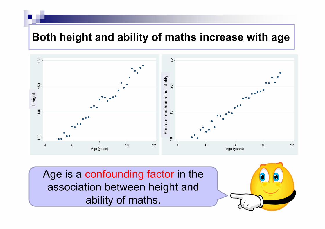
Both height and ability of maths increase with age13

014

015

016

0H

EIG

HT

4 6 8 10 12Age (years)

1015

2025

Scor

e of

mat

hem

atic

al a

bilit

y

4 6 8 10 12Age (years)

Age is a confounding factor in the association between height and

ability of maths.

Scor

e of

mat

hem

atic

al a

bilit

y

Hei

ght

How age itself influences the association between height and the ability of maths?

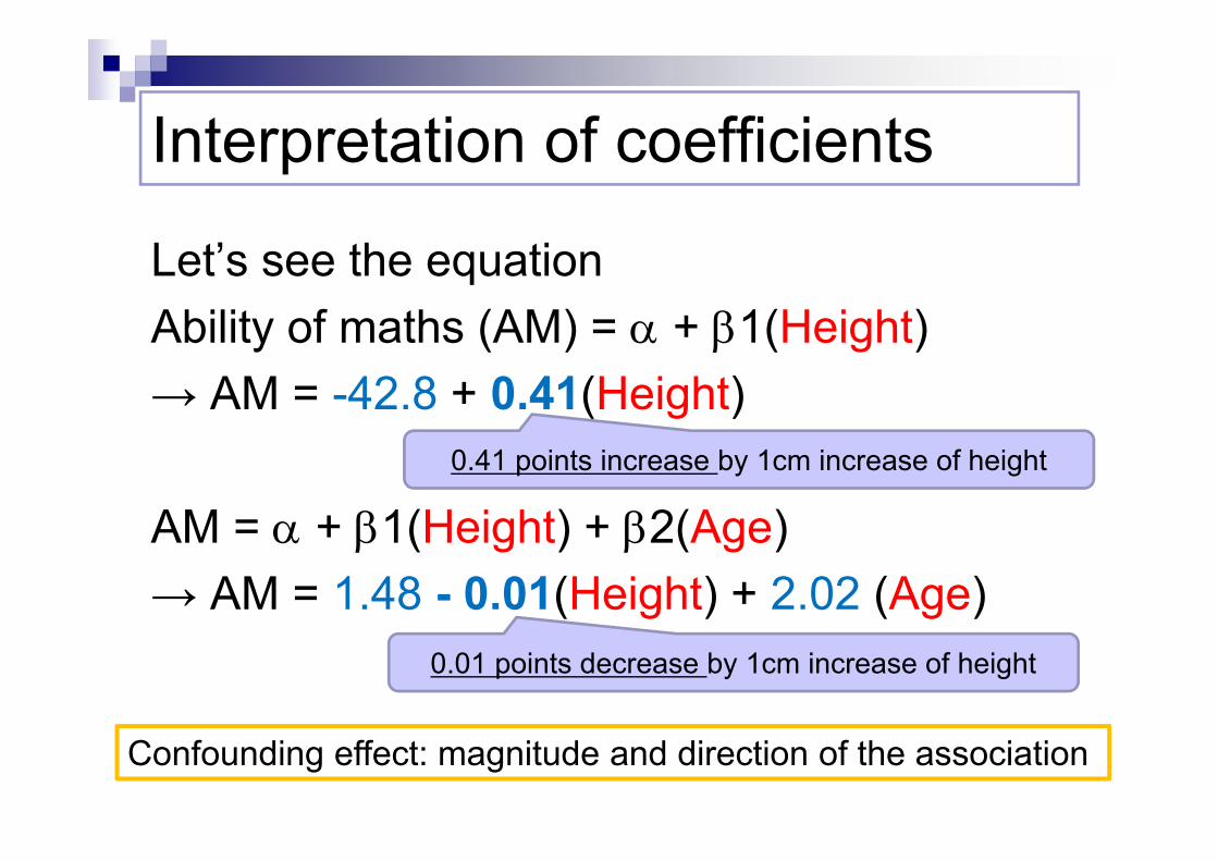
Let’s see the equation Ability of maths (AM) = + 1(Height) → AM = -42.8 + 0.41(Height)

AM = + 1(Height) + 2(Age)→ AM = 1.48 - 0.01(Height) + 2.02 (Age)

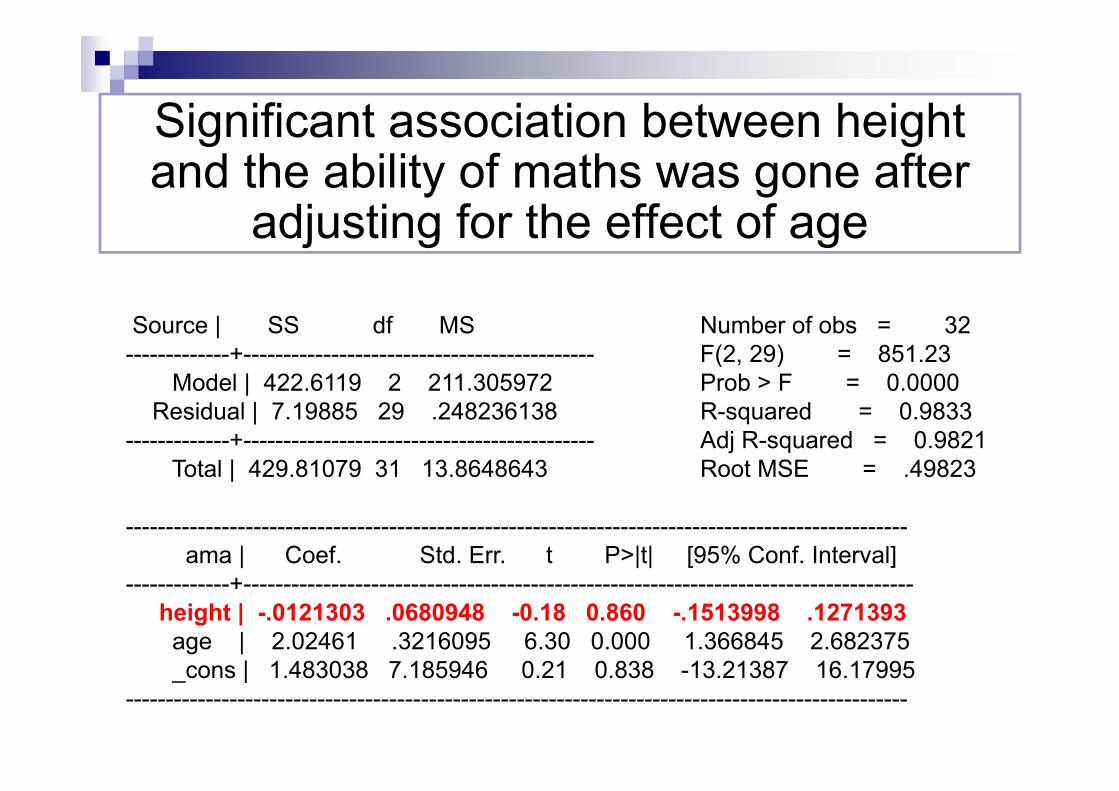
Significant association between height and the ability of maths was gone after

adjusting for the effect of age

Source | SS df MS Number of obs = 32-------------+-------------------------------------------- F(2, 29) = 851.23


-------------+-------------------------------------------- Adj R-squared = 0.9821Total | 429.81079 31 13.8648643 Root MSE = .49823

--------------------------------------------------------------------------------------------------ama | Coef. Std. Err. t P>|t| [95% Conf. Interval]

-------------+------------------------------------------------------------------------------------height | -.0121303 .0680948 -0.18 0.860 -.1513998 .1271393age | 2.02461 .3216095 6.30 0.000 1.366845 2.682375_cons | 1.483038 7.185946 0.21 0.838 -13.21387 16.17995

--------------------------------------------------------------------------------------------------

1015

2025

var6

130 140 150 160HEIGHT

No association between height and age-adjusted score of mathsAg

e-ad

just

ed s

core

of m

athe

mat

ical

abi

lity

Interpretation of coefficients

Let’s see the equation Ability of maths (AM) = + 1(Height) → AM = -42.8 + 0.41(Height)


0.41 points increase by 1cm increase of height

0.01 points decrease by 1cm increase of height

Confounding effect: magnitude and direction of the association

Source | SS df MS Number of obs = 32-------------+-------------------------------------------- F(2, 29) = 851.23


-------------+-------------------------------------------- Adj R-squared = 0.9821Total | 429.81079 31 13.8648643 Root MSE = .49823

--------------------------------------------------------------------------------------------------ama | Coef. Std. Err. t P>|t| [95% Conf. Interval]

-------------+------------------------------------------------------------------------------------height | -.0121303 .0680948 -0.18 0.860 -.1513998 .1271393age | 2.02461 .3216095 6.30 0.000 1.366845 2.682375_cons | 1.483038 7.185946 0.21 0.838 -13.21387 16.17995

--------------------------------------------------------------------------------------------------

Sum of Squares

Degrees of freedom

Mean sum of squares (SS/df)

ANOVA table

F statistic(dfm, dfr)

P value of F test

t = Coef. / SEt = Coef. / SE P value (H0: coef.=0) P value (H0: coef.=0)

CI of Coef.

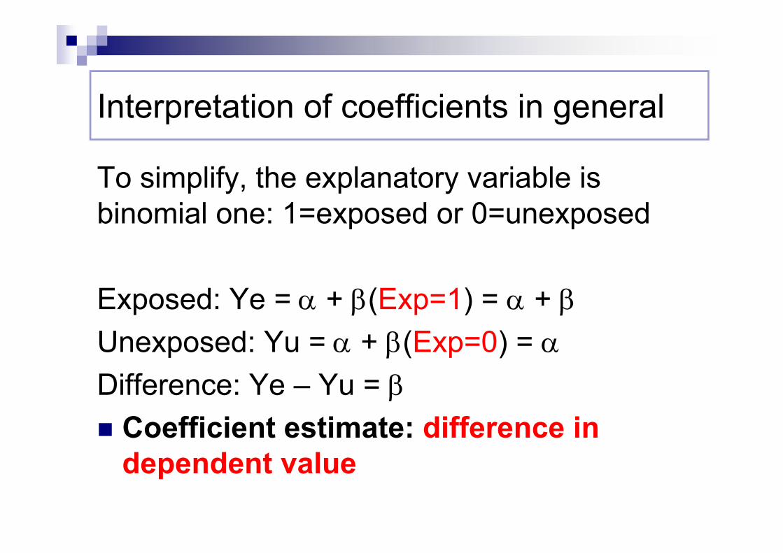
To simplify, the explanatory variable is binomial one: 1=exposed or 0=unexposed

Exposed: Ye = + (Exp=1) = + Unexposed: Yu = + (Exp=0) = Difference: Ye – Yu = Coefficient estimate: difference in

dependent value

Interpretation of coefficients in general

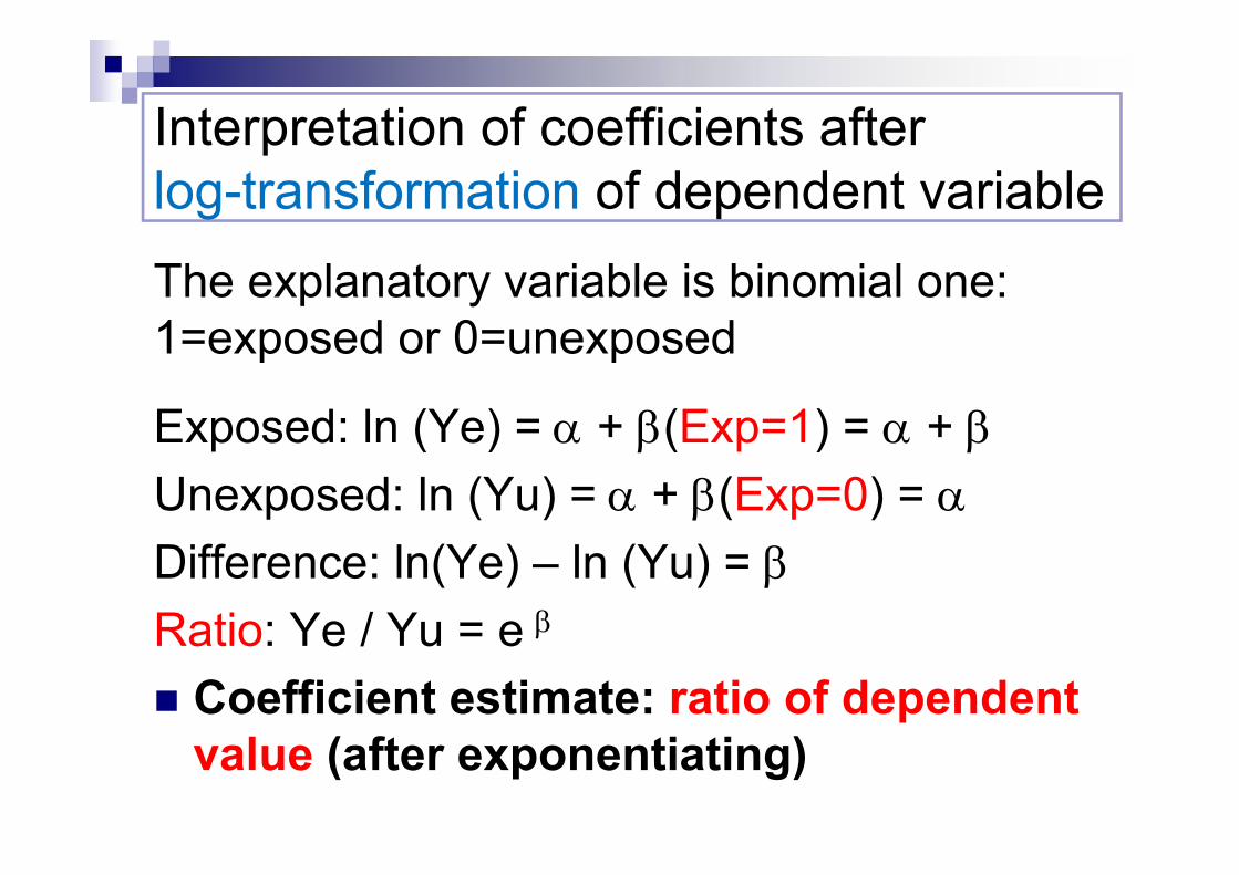
The explanatory variable is binomial one: 1=exposed or 0=unexposed

Exposed: ln (Ye) = + (Exp=1) = + Unexposed: ln (Yu) = + (Exp=0) = Difference: ln(Ye) – ln (Yu) = Ratio: Ye / Yu = e

Coefficient estimate: ratio of dependent value (after exponentiating)

Interpretation of coefficients after log-transformation of dependent variable

Control of confounding with regression model Compared to stratified analysis, several

confounding variables can be easily controlled simultaneously using a multivariable regression model.

Results from the regression model are readily susceptible to bias if the model is not a good fit to the data.

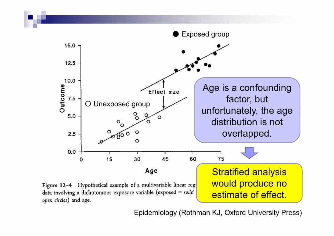
Epidemiology (Rothman KJ, Oxford University Press)

Age is a confounding factor, but

unfortunately, the age distribution is not

overlapped.

● Exposed group

〇 Unexposed group

Stratified analysis would produce no estimate of effect.

Epidemiology (Rothman KJ, Oxford University Press)

● Exposed group

〇 Unexposed group

Although the age distribution is not

overlapped, a regression model will fit two parallel straight lines through the

data.

CORRELATION = REGRESSION ANALYSIS?

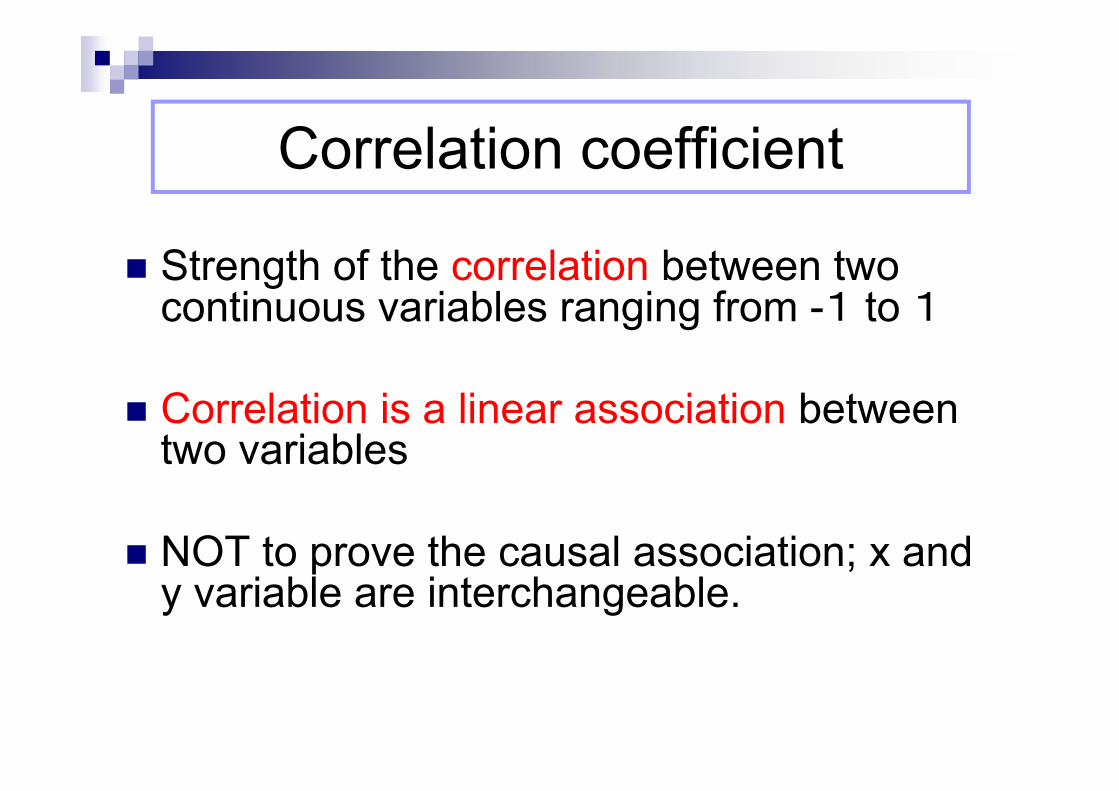
Correlation coefficient

Strength of the correlation between two continuous variables ranging from -１ to １

Correlation is a linear association between two variables

NOT to prove the causal association; x and y variable are interchangeable.

Examples of correlation

X

0

20

40

60

80

100

0 50 100

X

0

20

40

60

80

100

0 50 100

r = 1 r = -1

Positively correlated Negatively correlated

What does “r=0” mean? No association between x and y？ No linear association between x and y

0

2

4

6

8

10

12

14

16

18

0 2 4 6 8 10

X

Y

X

0

20

40

60

80

100

0 50 100

Correlation coefficient is not the magnitude of “slope”

Strong correlation Weak correlation

Correlation coefficients

Pearson’s CC (r)：parametric methodAt least, one of the two variables should

follow the normal distribution.

Non-parametric methodsSpearman’s CC ()Kendall’s CC ()

r (correlation coefficient) and R-squared30

4050

6070

80W

eigh

t

r = 0.44810.4481 x 0.4481=?

R2 = r2

2

R2 = 1-2

R squared, coefficient of determination, is the proportion of the variance in the dependent variable that is predictable from the independent variable(s).

r (correlation coefficient) and R-squared30

4050

6070

80W

eigh

t

The R2 coefficient of determination, ranging 0-1, is a statistical measure of how well the regression predictions approximatethe real data points.

Adjusted R squared value by the sample size and the number of

variable(s)Better to use when you have more

variables or small sample sizeW = -40 + 0.6084xH

r (correlation coefficient) and regression coefficient30

4050

6070

80W

eigh

t

r = 0.4481P<0.001

3040

5060

7080

Wei

ght W = -40 + 0.6084xH

130

140

150

160

170

Hei

ght

H = 133 + 0.3301xW

Regression coefficient

√0.6084 x 0.3301=0.4481

ADJUSTMENT OF CORRELATION

age weight calculation6.2 24.8 1348.6 25.6 1363.9 15.9 1174.7 16.1 1247.7 24.2 1378.8 28.9 1358.7 31.8 1357.3 22.3 1375.6 18.9 1312.5 15 100

Calculation skill and physical development

Is weight related to calculation

skill?

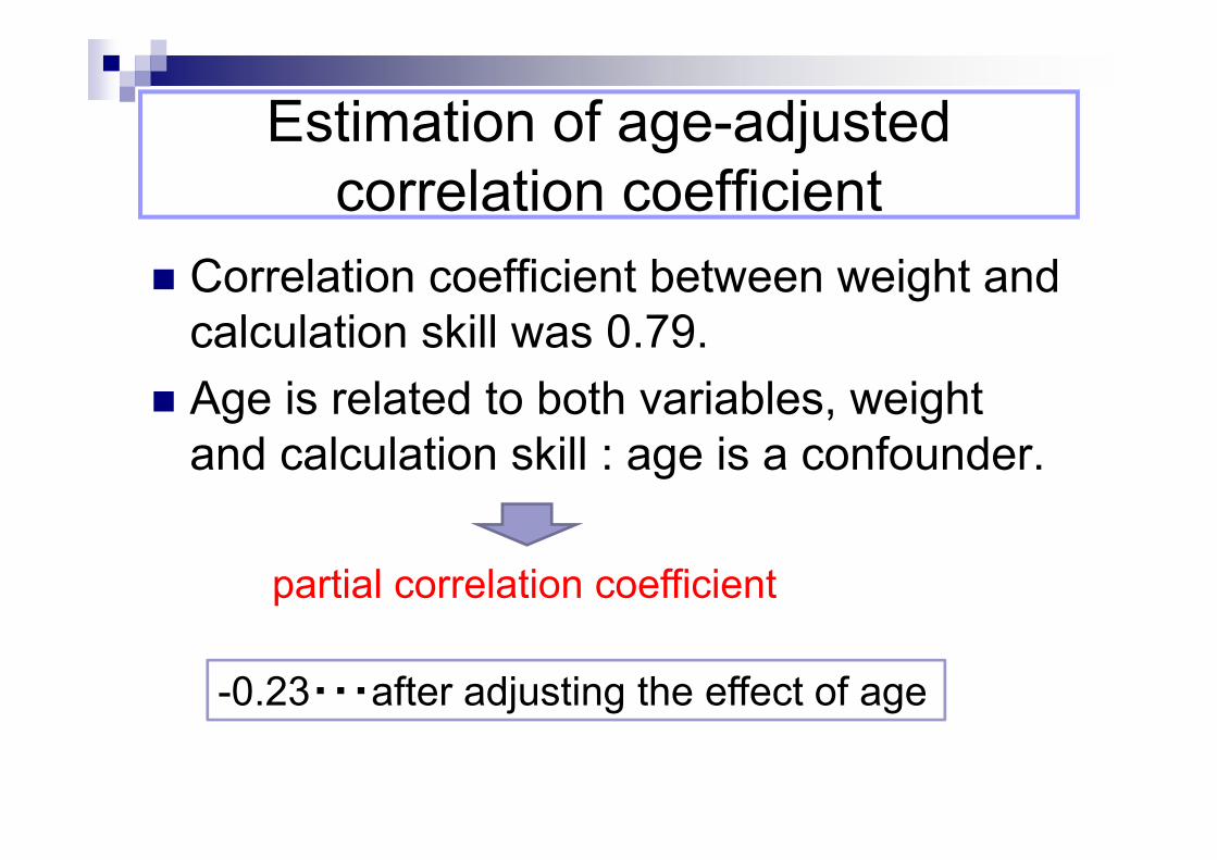
Correlation coefficient between weight and calculation skill was 0.79.

Age is related to both variables, weight and calculation skill : age is a confounder.

Estimation of age-adjusted correlation coefficient

partial correlation coefficient

-0.23・・・after adjusting the effect of age

Multivariate ≠ Multivariable (Multiple)

Multivariable (Multiple) analysis

This is the model to control the effects of confounders!

Multivariate analysis

This model is to analyze the relationship between “multiple outcomes” and a single set of

predictors.

LOGISTIC REGRESSION ANALYSIS

Logistic regression analysis Logistic regression is used to model the

probability of a binary response as a function of a set of variables thought to possibly affect the response (called covariates).

1: case (with the disease)Y =

0: control (no disease)

One could imagine trying to fit a linear model (since this is the simplest model !) for the probabilities, but often this leads to problems:

In a linear model, fitted probabilities can fall outside of 0 to 1. Because of this, linear models are seldom used to fit probabilities.

00.20.40.60.8

11.21.41.6

10 20 30 40

logistic modelProbability

In a logistic regression analysis, the logit of the probability is modeled, rather than the probability itself.

P = probability of getting disease (0～1)p

logit (p) = log1-p

As always, we use the natural log. The logit is therefore the log odds, since odds = p / (1-p)

This transformation allows us to use a linear model.

Logistic regression model

Now, we have the same function with linearregression model in the right side.

pxlogit (px) = log = + x

1 – pxwhere px = probability of event for a given value x, and and are unknown parameters to be estimated from the data.→ Multivariable analysis is applicable to adjust the effect of confounding factor.

The explanatory variable is binomial one: 1=exposed or 0=unexposed

Exposed: log (Oe) = + (Exp=1) = + Unexposed: log (Ou) = + (Exp=0) = Difference: log(Oe) – log (Ou) = Odds ratio: Oe / Ou = e

Coefficient estimate: Odds ratio (after exponentiating)

Interpretation of coefficients of logistic regression model

SURVIVAL ANALYSIS

Survival time：from the entry point（for example, when the treatment starts） until end point（for example, disease recurrence or the death from the disease）

Censoring: the follow-up is stopped because of other reason (for example, study period is over or the death from other reason）

Survival analysis

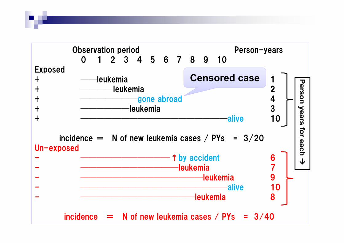
Observation period Person-years0 1 2 3 4 5 6 7 8 9 10

Exposed+ ──leukemia 1+ ────leukemia 2+ ───────gone abroad 4+ ──────leukemia 3+ ──────────────────alive 10

incidence ＝ N of new leukemia cases / PYs = 3/20Un-exposed- ───────────☨by accident 6- ────────────leukemia 7- ───────────────leukemia 9- ──────────────────alive 10- ──────────────leukemia 8

incidence ＝ N of new leukemia cases / PYs = 3/40

Person years for each

Censored case

0.2

5.5

.75

1

0 5 10analysis time

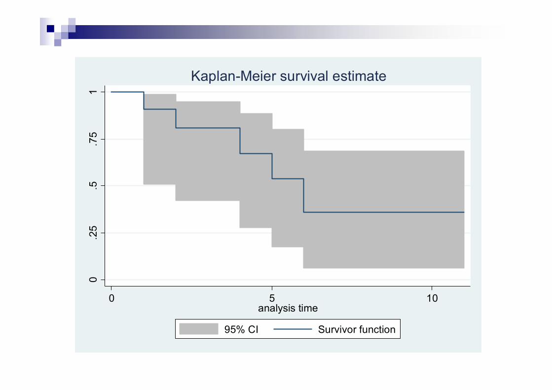
95% CI Survivor function

Kaplan-Meier survival estimate

0.2

5.5

.75

1

0 5 10analysis time

95% CI 95% CIa b

Kaplan-Meier survival estimates

P=0.016

The statistic follows the chi-square distribution (df=1)

Log-rank test:Statistic test for the difference of survival probability

Limitations of Kaplan-Meier method

Mainly descriptiveDoesn’t control for covariatesRequires categorical predictors Can’t accommodate time-dependent

variables

This model is expressed by the following formula; where λ(t) is the hazard of variable xk and t is the time until the case is alive, and λ0(t) is the baseline hazard. We assume that the log of hazard ratio is proportional to the variable X.

Hazard ratio: λ1(t)/λ0 (t)=exp(β)


Exposed group Un-exposed group

Log negative-log plot is useful to check

Group A=1, Group B=0No. of subjects = 22 Number of obs = 22No. of failures = 15Time at risk = 77

LR chi2(1) = 4.68Log likelihood = -35.943457 Prob > chi2 = 0.0305-------------------------------------------------------------------------------------------------

_t | Haz. Ratio Std. Err. z P>|z| [95% Conf. Interval]-------------+----------------------------------------------------------------------------------

A | 0.29 0.1767 -2.04 0.042 0.0895 0.9557-------------------------------------------------------------------------------------------------

STRATEGY FOR CONSTRUCTING REGRESSION MODELS

Basic principles

1. Stratified analysis should be first.2. Determine which confounders to

include in the model.3. Estimate the shape of the exposure-

disease relation. Dose-response relation

4. Evaluate interaction

How to determine confounders: data-dependent manner1. Start with a set of predictors of outcome

based on the strength of their relation to the outcome.

2. Build a model by introducing predictor variables one at a time: check the amount of change in the coefficient of the exposure term

> 10% change: include it as a confounder

Example of a confounder (age)

Ability of maths (AM) = + 1(Height) → AM = -42.8 + 0.41(Height)


> 10% change

How to determine confounders: data-independent mannerSome researchers argue that “Without data analysis, decide confounders, important risk factors of the outcome, based on the previous studies.”

How can we pick-up “important risk factors”?If there are few studies, how can we know confounders?

How many explanatory variables can we use in a model?Model Number of explanatory

variablesExample

Linear regression model

Sample size / 15 Up to around 6-7 variables in 100 subjects

Logistic regression model

Smaller sample size of outcome /10

Up to 10 variables if the numbers of cases and controls are 100 and 300, respectively.


The number of event / 10

Up to 9 variables if you have 90 events out of 150 subjects

ATTENTION!

When you include a categorical variable in your model, you have to count that as “the number of categories – 1”.

For example, the variable of age group used in the previous practice, we have to count it as “two” (=3 categories -1) variables.

PROPENSITY SCORE

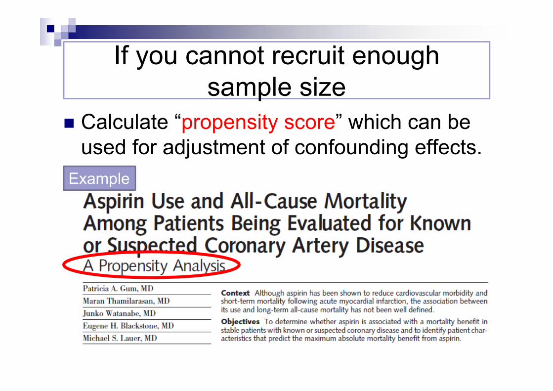
If you cannot recruit enough sample size

Calculate “propensity score” which can be used for adjustment of confounding effects.

Example

Almost all prognostic factors (n=28) are

related to aspirin use!

After matching by propensity score, the distribution of prognostic factors are similar

between aspirin users and non-users.

It is just like a RCT! (pseud RCT)

You need to include only

propensity score in the model.

WE SHOULD NOT RELY ON P VALUE TOO MUCH

Statistic significance vs. Clinical significance

Statistic significance ≠ Clinical significance

P value(s) do NOT tell us the significance in clinical practice / biological importance.

If your sample size is quite large, you may obtain a result with statistic significance. So what?

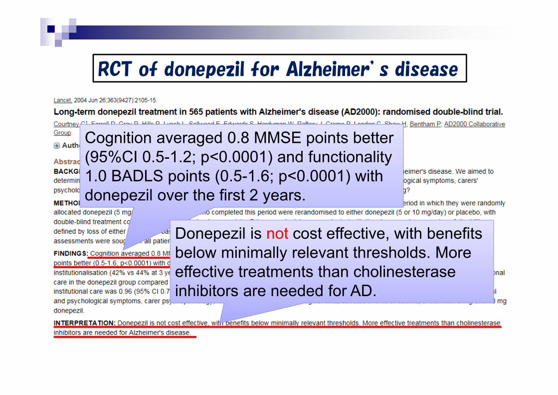
RCT of donepezil for Alzheimer’s disease

Cognition averaged 0.8 MMSE points better (95%CI 0.5-1.2; p<0.0001) and functionality 1.0 BADLS points (0.5-1.6; p<0.0001) with donepezil over the first 2 years.

Donepezil is not cost effective, with benefits below minimally relevant thresholds. More effective treatments than cholinesterase inhibitors are needed for AD.

In a RCT study, the mortality rates of new drug A and old drug B were 30% and 20%, respectively. And, the p value was 0.6 for the difference of them.

１．The mortality rate of drug A is equivalent to that of drug B.

２．We cannot say “there is a difference in the mortality between drug A and B”.

３．We cannot say “the mortality of drug A is higher than that of drug B”.

Which description is appropriate?

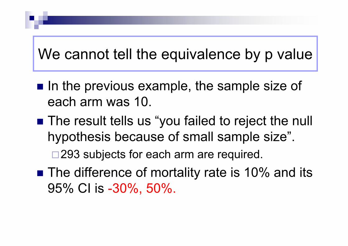
In the previous example, the sample size of each arm was 10.

The result tells us “you failed to reject the null hypothesis because of small sample size”.293 subjects for each arm are required.

The difference of mortality rate is 10% and its 95% CI is -30%, 50%.

We cannot tell the equivalence by p value

American Statistical Association Releases Statement on Statistical Significance and P-valuesProvides Principles to Improve the Conduct and Interpretation of Quantitative Sciencehttps://www.amstat.org/newsroom/pressreleases/P-ValueStatement.pdf

1. P-values can indicate how incompatible the data are with a specified statistical model.

2. P-values do not measure the probability that the studied hypothesis is true, or the probability that the data were produced by random chance alone.

3. Scientific conclusions and business or policy decisions should not be based only on whether a p-value passes a specific threshold.

4. Proper inference requires full reporting and transparency.5. A p-value, or statistical significance, does not measure the size of

an effect or the importance of a result.6. By itself, a p-value does not provide a good measure of evidence

regarding a model or hypothesis.

multivariable analysis: a brief introduction 21am... · why do we need multivariable analysis?...

Documents