Multivariate Analysis of Variance, Part 2

BMTRY 7262/21/14

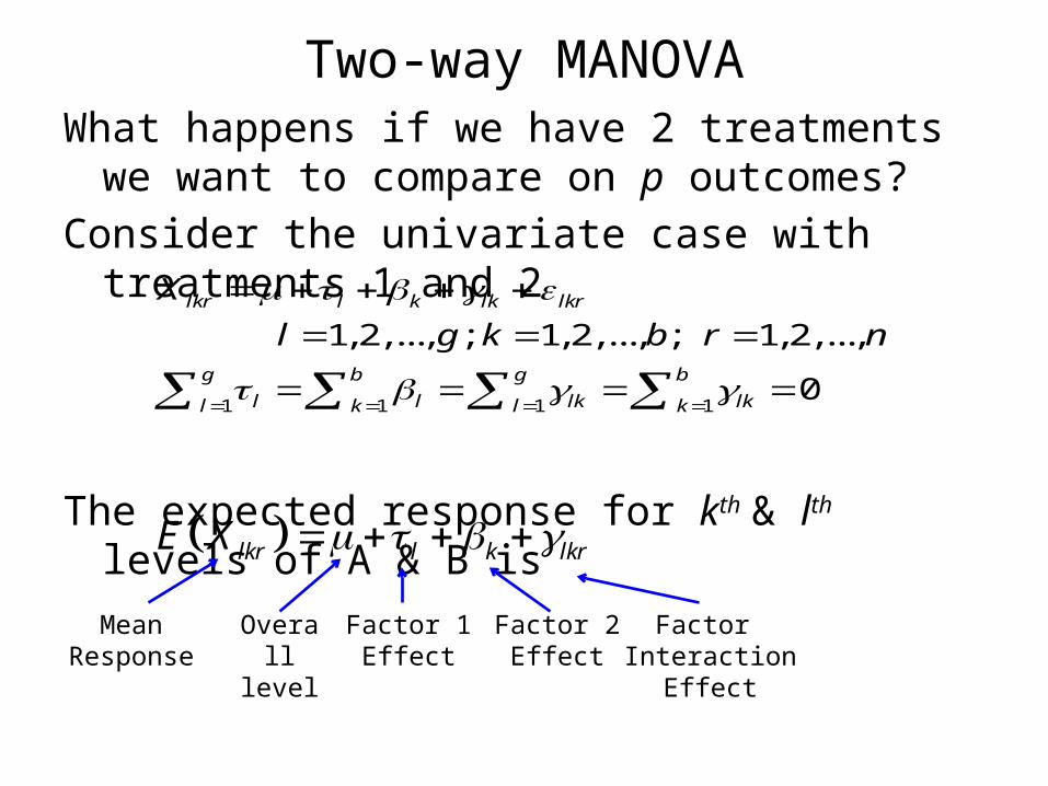
Two-way MANOVAWhat happens if we have 2 treatments we want to

compare on p outcomes?Consider the univariate case with treatments 1 and 2

The expected response for kth & lth levels of A & B is

1 1 1 1

1,2,..., ; 1, 2,..., ; 1, 2,...,

0

lkr l k lk lkr

g b g b

l l lk lkl k l k

X

l g k b r n

lkr l k lkrE X

MeanResponse

Overalllevel

Factor 1Effect

Factor 2Effect

Factor Interaction

Effect

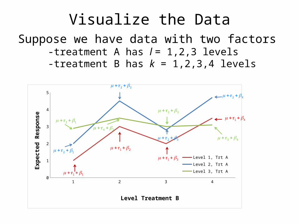
Visualize the DataSuppose we have data with two factors -treatment A has l = 1,2,3 levels -treatment B has k = 1,2,3,4 levels

1 2 3 40

1

2

3

4

5

Level Treatment B

Level 1, Trt A

Level 2, Trt A

Level 3, Trt A

Expe

cted

Res

pons

e

2 1

3 3

1 1

1 2

1 3

1 4 3 1

4 2

3 4

2 2

2 3

2 4

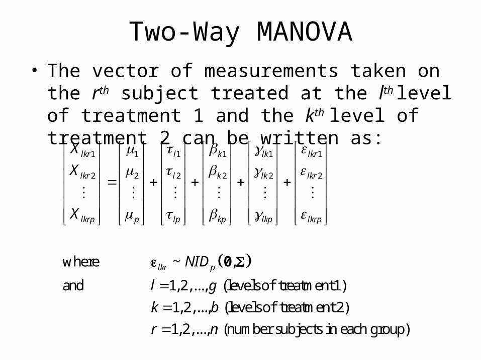
Two-Way MANOVA• The vector of measurements taken on the rth subject

treated at the lth level of treatment 1 and the kth level of treatment 2 can be written as:

1 1 1 1 1 1

2 2 2 2 2 2

where ~ ,

and 1,2,..., (levels o

lkr l k lk lkr

lkr l k lk lkr

lkrp p lp kp lkp lkrp

lkr p

X

X

X

NID

l g

0

f treatment1)

1,2,..., (levels of treatment 2)

1,2,..., (number subjects in each group)

k b

r n

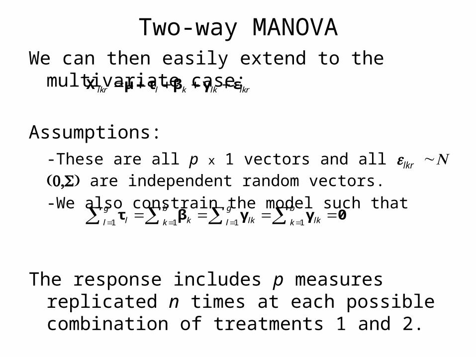
Two-way MANOVAWe can then easily extend to the multivariate case:

Assumptions:-These are all p x 1 vectors and all elkr ~ N (0,S) are independent random vectors.-We also constrain the model such that

The response includes p measures replicated n times at each possible combination of treatments 1 and 2.

lkr l k lk lkr X μ τ β γ ε

1 1 1 1

g b g b

l k lk lkl k l k τ β γ γ 0

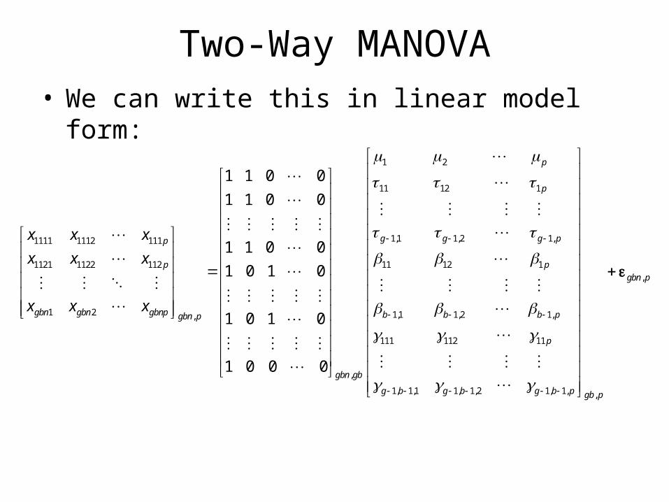
Two-Way MANOVA• We can write this in linear model form:

1 2

11 12 1

1,1 1,2 1,1111 1112 111

1121 1122 112 11 12 1

1 2 ,

,

1 1 0 0

1 1 0 0

1 1 0 0

1 0 1 0

1 0 1 0

1 0 0 0

p

p

g g g pp

p

gbn gbn gbnp gbn p

gbn gb

x x x

x x x

x x x

,

1,1 1,2 1,

111 112 11

1, 1,1 1, 1,2 1, 1, ,

p

gbn p

b b b p

p

g b g b g b p gb p

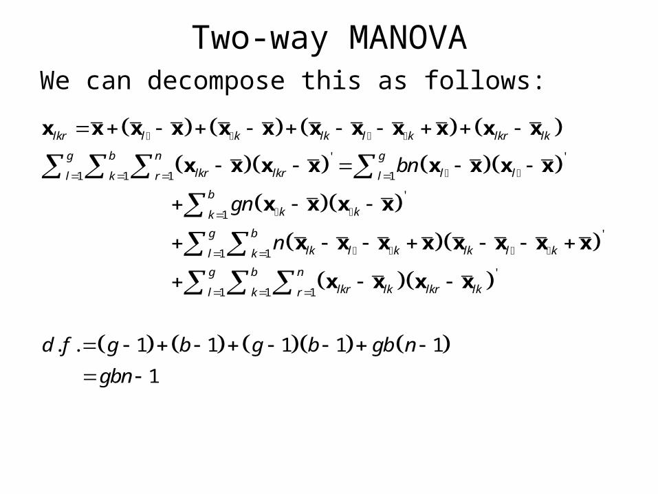
Two-way MANOVAWe can decompose this as follows:

' '

1 1 1 1

'

1

'

1 1

'

1 1 1

. . 1 1 1 1

lkr l k lk l k lkr lk

g b n g

lkr lkr l ll k r l

b

k kk

g b

lk l k lk l kl k

g b n

lkr lk lkr lkl k r

bn

gn

n

d f g b g b g

x x x x x x x x x x x x

x x x x x x x x

x x x x

x x x x x x x x

x x x x

1

1

b n

gbn

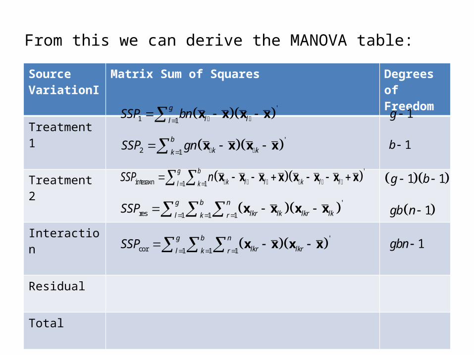
From this we can derive the MANOVA table:

SourceVariationI

Matrix Sum of Squares Degrees of Freedom

Treatment 1

Treatment 2

Interaction

Residual

Total

'

1 1

g

l llSSP bn

x x x x

'

interaxn 1 1

g b

k l l k l ll kSSP n

x x x x x x x x

'

2 1

b

k kkSSP gn

x x x x

'

res 1 1 1

g b n

lkr lk lkr lkl k rSSP

x x x x

'

cor 1 1 1

g b n

lkr lkrl k rSSP

x x x x

1g

1b

1 1g b

1gb n

1gbn

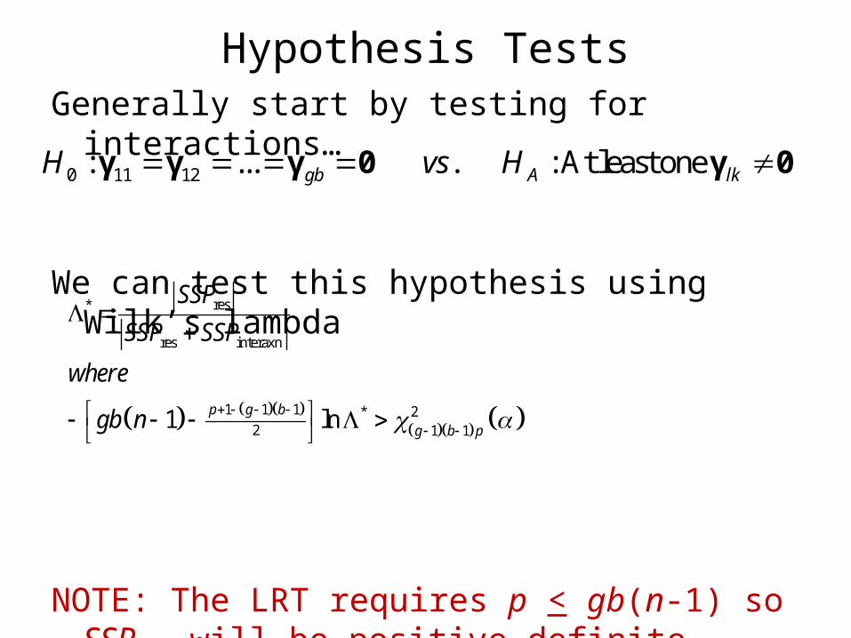
Hypothesis TestsGenerally start by testing for interactions…

We can test this hypothesis using Wilk’s lambda

NOTE: The LRT requires p < gb(n-1) so SSPres will be positive definite

0 11 12: ... . : At least onegb A lkH vs H γ γ γ 0 γ 0

res*

res interaxn

1 1 1 * 22 1 11 lnp g b

g b p

SSP

SSP SSP

where

gb n

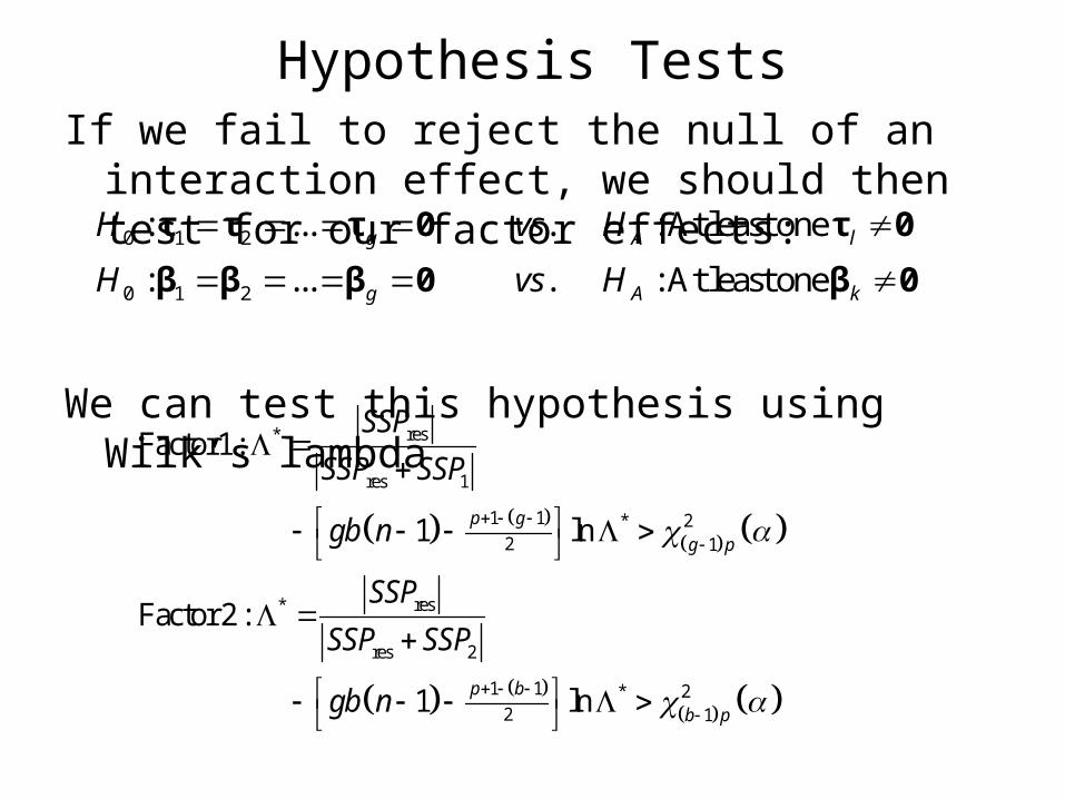
Hypothesis TestsIf we fail to reject the null of an interaction effect, we

should then test for our factor effects:

We can test this hypothesis using Wilk’s lambda

0 1 2

0 1 2

: ... . : At least one

: ... . : At least one

g A l

g A k

H vs H

H vs H

τ τ τ 0 τ 0

β β β 0 β 0

res*

res 1

1 1 * 22 1

res*

res 2

1 1 * 22 1

Factor1:

1 ln

Factor 2 :

1 ln

p g

g p

p b

b p

SSP

SSP SSP

gb n

SSP

SSP SSP

gb n

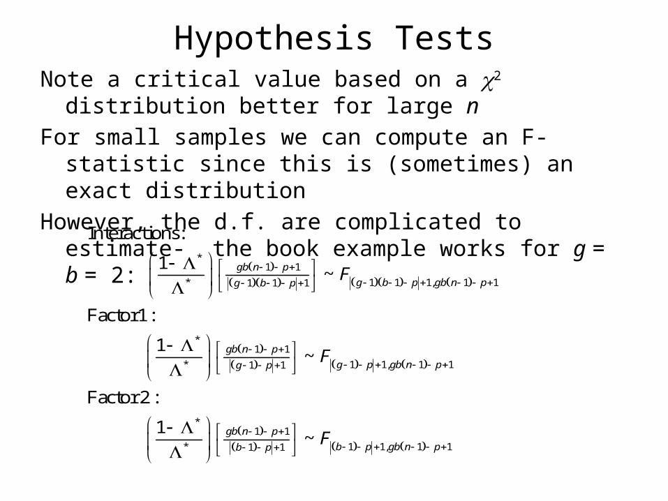
Hypothesis TestsNote a critical value based on a c2 distribution better for large nFor small samples we can compute an F-statistic since this is

(sometimes) an exact distributionHowever, the d.f. are complicated to estimate- the book

example works for g = b = 2:

*1 1

* 1 1 1, 1 11 1 1

*1 1

* 1 1, 1 11 1

*1 1

* 1 1, 1 11 1

Interactions:

1~

Factor1:

1~

Factor 2 :

1~

gb n p

g b p gb n pg b p

gb n p

g p gb n pg p

gb n p

b p gb n pb p

F

F

F

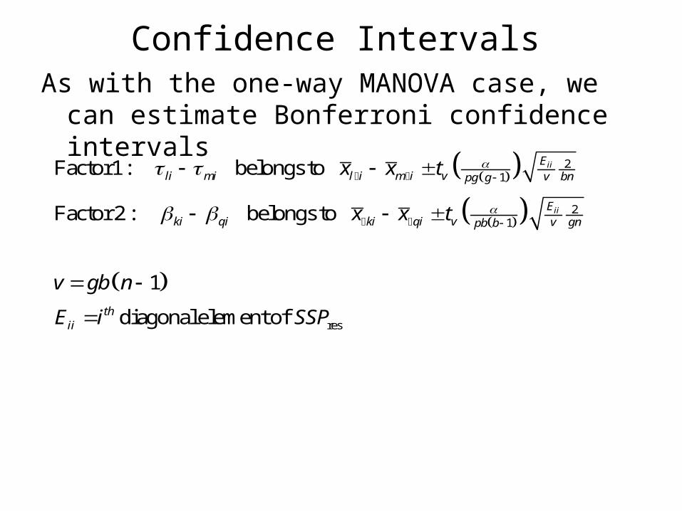
Confidence IntervalsAs with the one-way MANOVA case, we can estimate

Bonferroni confidence intervals

21

21

res

Factor1: belongs to

Factor 2 : belongs to

1

diagonalelement of

ii

ii

Eli mi l i m i v v bnpg g

Eki qi ki qi v v gnpb b

thii

x x t

x x t

v gb n

E i SSP

Example: Cognitive impairment in Parkinson’s Disease

It is known that lesions in the pre-frontal cortex are responsible for much of the motor dysfunction subject’s with Parkinson’s disease experience.

Cognitive impairment is a less well studied adverse outcome in Parkinson’s disease.

An investigator hypothesizes that lesions in the locus coeruleus region of the brain are in part responsible for this cognitive deficit.

The PI also hypothesizes that this is partly due to decreased expression of BDNF.

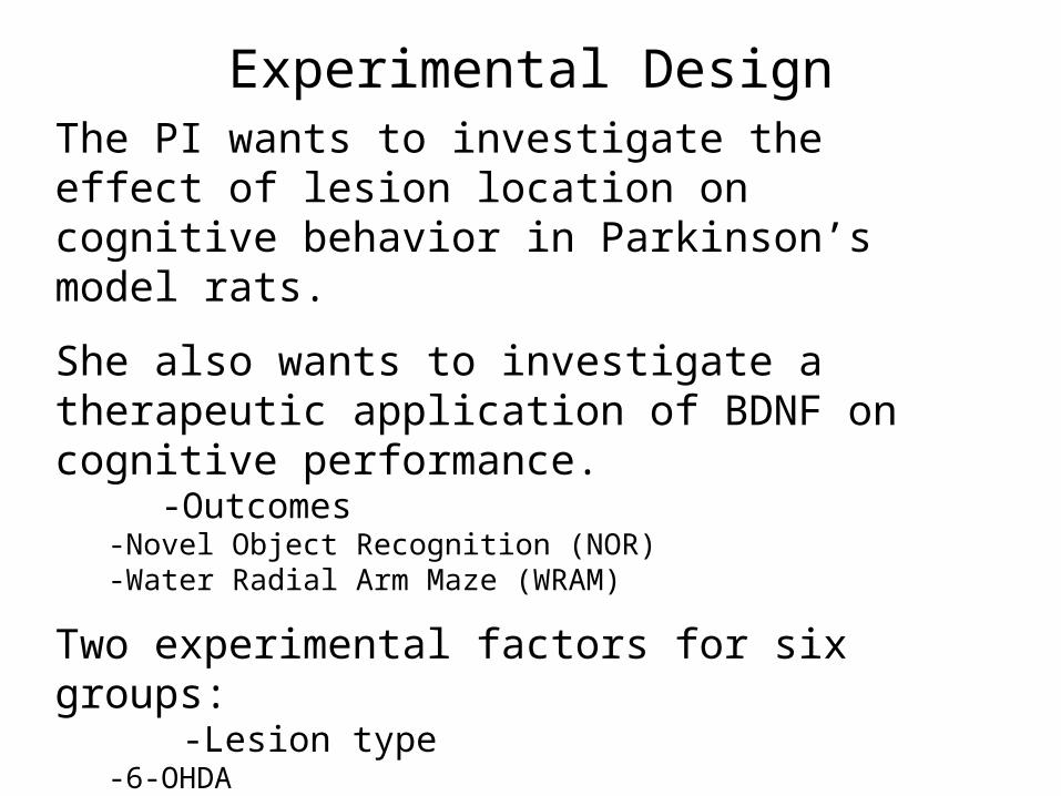
Experimental DesignThe PI wants to investigate the effect of lesion location on cognitive behavior in Parkinson’s model rats.

She also wants to investigate a therapeutic application of BDNF on cognitive performance. -Outcomes

-Novel Object Recognition (NOR)-Water Radial Arm Maze (WRAM)

Two experimental factors for six groups: -Lesion type

-6-OHDA-DSP-4-Double

-Therapy-BDNF microspheres-No treatment

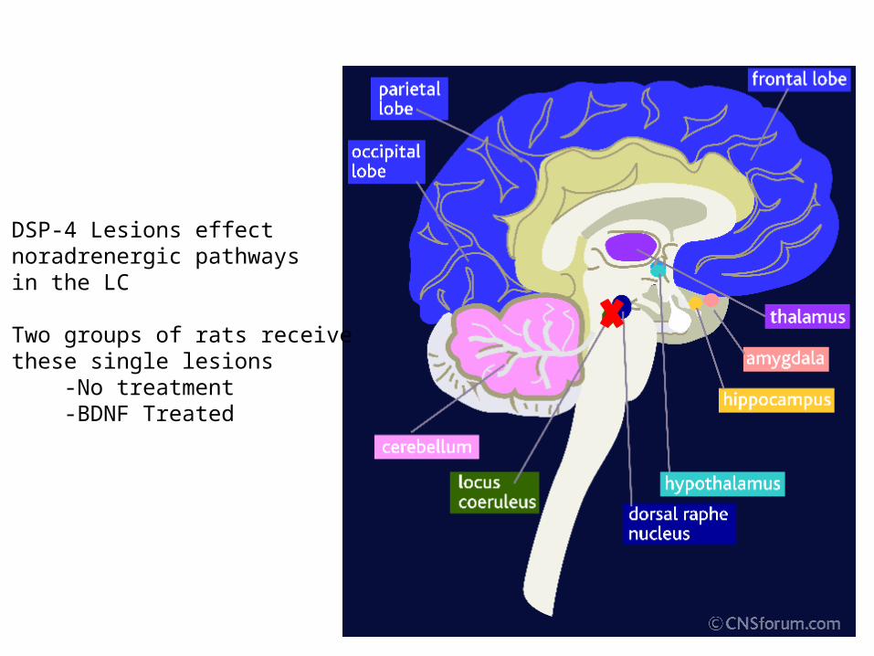
DSP-4 Lesions effect noradrenergic pathwaysin the LC

Two groups of rats receivethese single lesions -No treatment -BDNF Treated

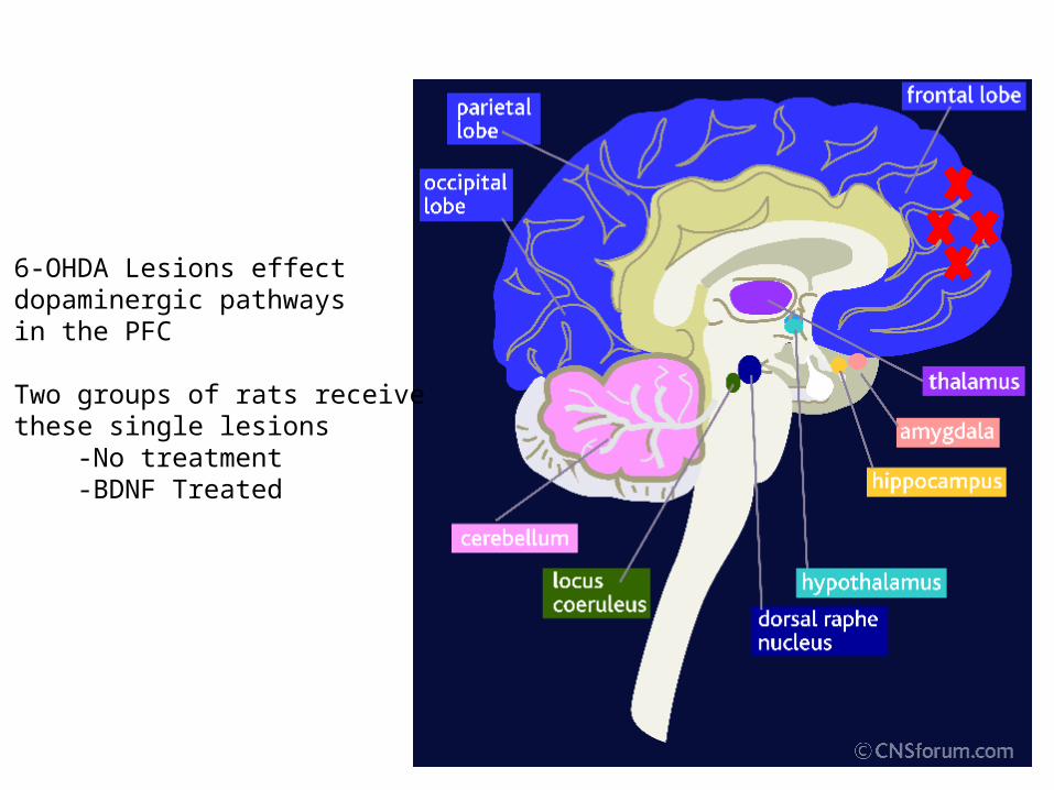
6-OHDA Lesions effect dopaminergic pathwaysin the PFC

Two groups of rats receivethese single lesions -No treatment -BDNF Treated

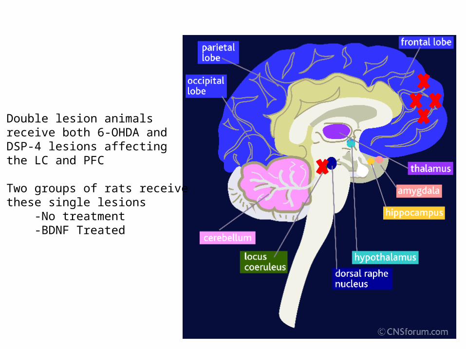
Double lesion animals receive both 6-OHDA andDSP-4 lesions affecting the LC and PFC

Two groups of rats receivethese single lesions -No treatment -BDNF Treated

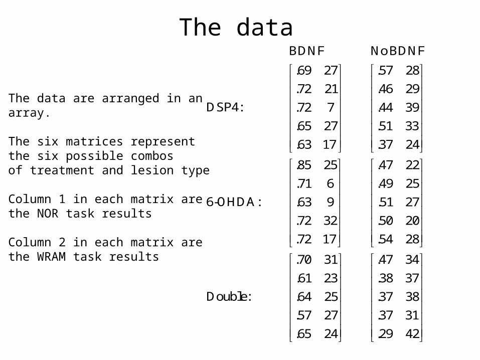
The dataBDNF No BDNF

.69 27 .57 28

.72 21 .46 29

DSP4: .72 7 .44 39

.65 27 .51 33

.63 17 .37 24

.85 25 .47 22

.71 6 .49 25

6-OHDA: .63 9 .51 27

.72 32 .50 20

.72 17 .54 28

.70 31

.61 23

Double:

.47 34

.38 37

.64 25 .37 38

.57 27 .37 31

.65 24 .29 42

The data are arranged in anarray.

The six matrices represent the six possible combosof treatment and lesion type

Column 1 in each matrix arethe NOR task results

Column 2 in each matrix arethe WRAM task results

Means for Sums of Squares

1, , 2

What is

What about Factor Factor

x

x x

Means for Sums of Squares

1, 2What about Factor Factorx

Sums of Squares1

2

What is the first term in

What is the first term in

factor

factor

SS

SS

Sums of Squares

intWhat is the first term in eractionSS

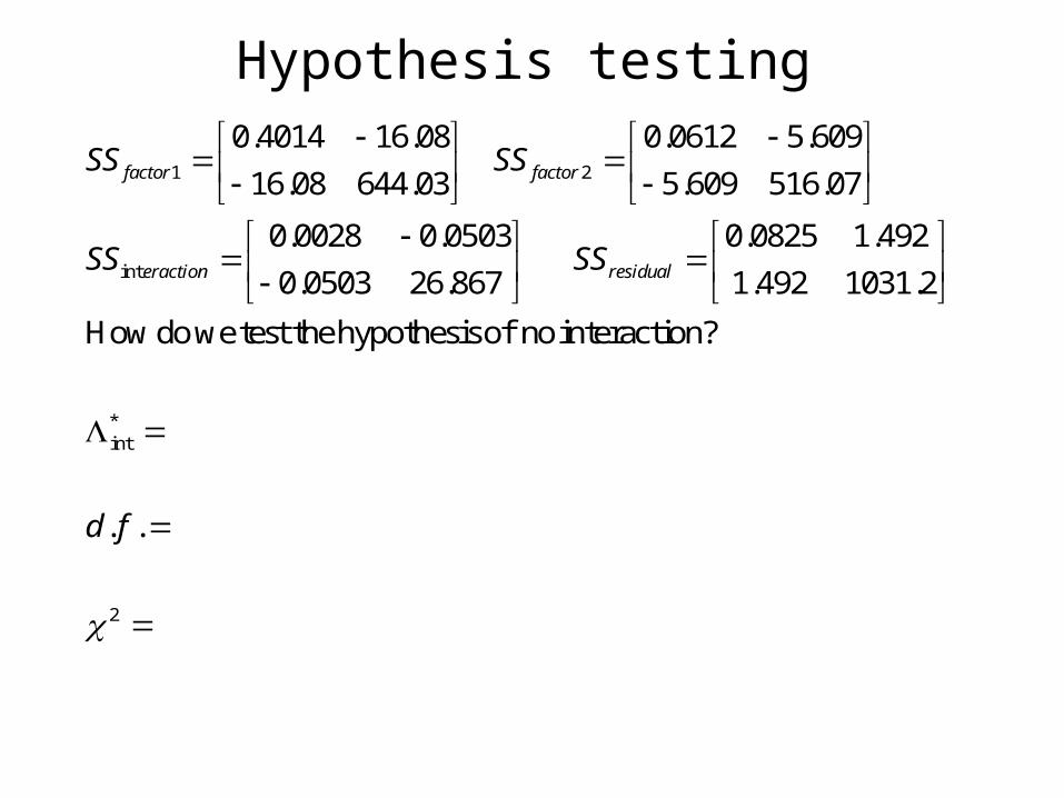
Hypothesis testing

1 2

int

0.4014 16.08 0.0612 5.609

16.08 644.03 5.609 516.07

0.0028 0.0503 0.0825 1.492

0.0503 26.867 1.492 1031.2

How do we test the hypothesis of nointerac

factor factor

eraction residual

SS SS

SS SS

*int

2

tion?

. .d f

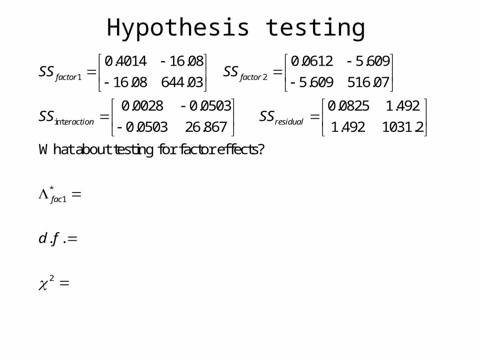
Hypothesis testing

1 2

int

0.4014 16.08 0.0612 5.609

16.08 644.03 5.609 516.07

0.0028 0.0503 0.0825 1.492

0.0503 26.867 1.492 1031.2

What about testing for factor effec

factor factor

eraction residual

SS SS

SS SS

*1

2

ts?

. .

fac

d f

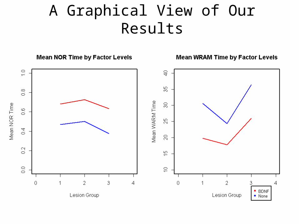
A Graphical View of Our Results

Bonferroni Simultaneous CIs

2

1 2 1 2 1 1 1

0.0825 1.492 0.6807 .4493, ,

1.492 1031.2 21.20 30.47

What are the 95% Bonferroni CI's for BDNF versus no BDNF?

NOR...

WRAM...

ii

residual BDNF NoBDNF

Ei i i i bngb n pg g gb n

SS

x x t

x x

Bonferroni Simultaneous CIs

4

1 2 1 2 1

0.0825 1.492 .576 .614 .505, , ,

1.492 1031.2 25.2 21.1 31.2

What are the 95% Bonferroni CI's for comparing different lesion types?

ˆ ˆ

residual DSP OHDA Doub

i i i i gb n p

SS

x x t

x x x

2

1 1

NOR in DSP4 vs 6OHDA...

WRAM in 6OHDA vs Double...

iiEgnb b gb n

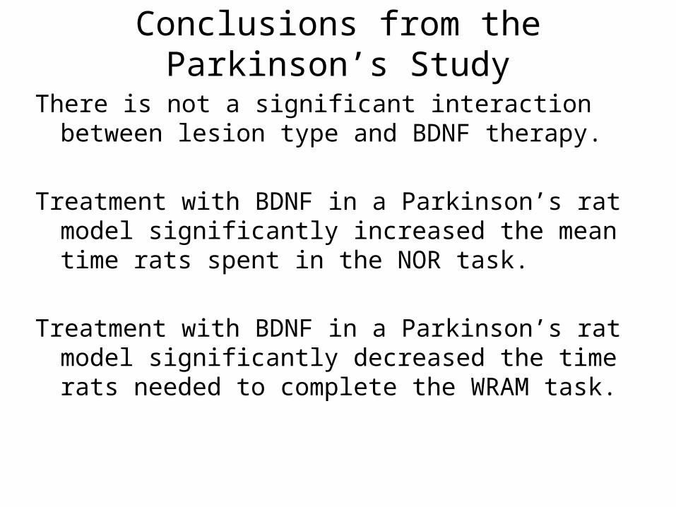
Conclusions from the Parkinson’s Study

There is not a significant interaction between lesion type and BDNF therapy.

Treatment with BDNF in a Parkinson’s rat model significantly increased the mean time rats spent in the NOR task.

Treatment with BDNF in a Parkinson’s rat model significantly decreased the time rats needed to complete the WRAM task.

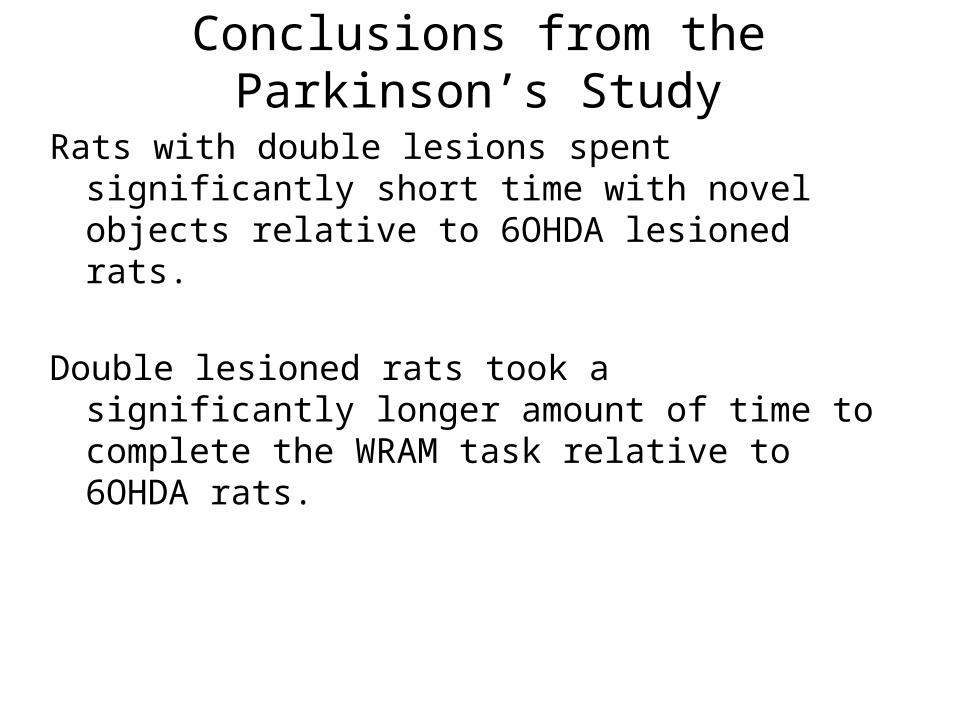
Conclusions from the Parkinson’s Study

Rats with double lesions spent significantly short time with novel objects relative to 6OHDA lesioned rats.

Double lesioned rats took a significantly longer amount of time to complete the WRAM task relative to 6OHDA rats.

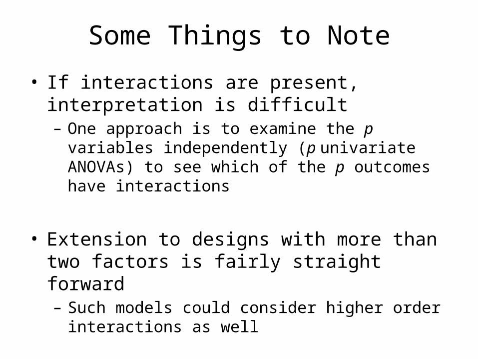
Some Things to Note

• If interactions are present, interpretation is difficult– One approach is to examine the p variables independently

(p univariate ANOVAs) to see which of the p outcomes have interactions

• Extension to designs with more than two factors is fairly straight forward– Such models could consider higher order interactions as

well