multivariate asset return prediction with mixture models but this is not the case! the same e ect...
TRANSCRIPT

Multivariate Asset Return Prediction with MixtureModels
Marc S. Paolella
Swiss Banking Institute, University of Zurich
Marc S. Paolella Multivariate Asset Return Prediction with Mixture Models

Introduction
The leptokurtic nature of asset returns has spawned an enormous amountof research into effective ways of modeling them, often involving the useof distributions which have power tails, and the ensuing nonexistence ofhigher moments.
−8 −6 −4 −2 0 2 4 6 80
0.05
0.1
0.15
0.2
0.25
0.3
Distribution of Stock Returns for Bank of America
kernel estimatefitted normal
Marc S. Paolella Multivariate Asset Return Prediction with Mixture Models

Introduction
This issue has long since transcended ivory tower academics andquantitative groups in financial institutions, especially since thestatement by Alan Greenspan (1997, p. 54),
... the biggest problems we now have with the whole evaluationof risk is the fat-tail problem, which is really creating very largeconceptual difficulties. Because as we all know, the assumptionof normality enables us to drop off a huge amount of complexityof our equations very much to the right of the equal sign.Because once you start putting in non-normality assumptions,which unfortunately is what characterizes the real worldwhich unfortunately is what characterizes the real worldwhich unfortunately is what characterizes the real world, thenthe issues become extremely difficult.
Marc S. Paolella Multivariate Asset Return Prediction with Mixture Models

Introduction
We propose a multivariate model which, besides exhibiting leptokurticbehavior and asymmetry,
lends itself to tractable distributions of weighted sums of themarginal random variables (to enable portfolio construction),
portfolios possess finite positive integer moments of all orders,
is super-fast to estimate,
delivers superior (compared to DCC and related models) multivariatedensity forecasts,
has trivial stationarity conditions as a stochastic process. This isaccomplished by not using a GARCH structure.
Marc S. Paolella Multivariate Asset Return Prediction with Mixture Models

Need for Mixtures
A mixture can capture, besides excess kurtosis and asymmetry, the twofurther stylized facts of
the leverage or down market effect—the negative correlationbetween volatility and asset returns, and
contagion effects—the tendency of the correlation between assetreturns to increase during pronounced market downturns, as well asduring periods of higher volatility.
Other fat-tailed multivariate distributions, such as the multivariateStudent’s t or the multivariate generalized hyperbolic distribution, cannotachieve this.
Marc S. Paolella Multivariate Asset Return Prediction with Mixture Models

Need for Mixtures
With a two-component multivariate normal mixture model withcomponent parameters µ1, Σ1, µ2, Σ2, we would expect to have theprimary component capturing the “business as usual” stock returnbehavior, with a near-zero mean vector µ1, and the second componentcapturing the more volatile, “crisis” behavior, with
(much) higher variances in Σ2 than in Σ1,
significantly larger correlations, reflecting the contagion effect,
and a predominantly negative µ2, reflecting the down market effect.
A distribution with only a single mean vector and covariance (or, moregenerally, dispersion) matrix cannot capture this behavior, no matter howmany additional shape parameters the distribution possesses.This is true even if each marginal were to be endowed with its own set ofshape (tail and skew) parameters, as is possible when using a copula.
Marc S. Paolella Multivariate Asset Return Prediction with Mixture Models
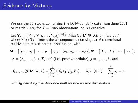
Evidence for Mixtures
We use the 30 stocks comprising the DJIA-30, daily data from June 2001to March 2009, for T = 1945 observations, on 30 variables.
Let Yt = (Yt,1,Yt,2, . . . ,Yt,d)′i.i.d.∼ MixkNd(M,Ψ,λ), t = 1, . . . ,T ,
where MixkNd denotes the k-component, non-singular d-dimensionalmultivariate mixed normal distribution, with
M =[µ1 µ2 · · · µk
], µj = (µ1j , µ2j , . . . , µdj)
′, Ψ =[
Σ1 Σ2 · · · Σk
],
λ = (λ1, . . . , λk), Σj > 0 (i.e., positive definite), j = 1, . . . , k , and
fMixkNd(y; M,Ψ,λ) =
k∑
j=1
λj fN(y;µj ,Σj
), λj ∈ (0, 1),
k∑
j=1
λj = 1,
with fN denoting the d-variate multivariate normal distribution.
Marc S. Paolella Multivariate Asset Return Prediction with Mixture Models
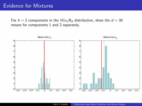
Evidence for Mixtures
For k = 2 components in the MixkNd distribution, show the d = 30means for components 1 and 2 separately.
−0.4 −0.3 −0.2 −0.1 0 0.1 0.2 0.3 0.40
1
2
3
4
5
6
7
8
9
Means from μ1
−0.4 −0.3 −0.2 −0.1 0 0.1 0.2 0.3 0.40
1
2
3
4
5
6
7
8
9
Means from μ2
Marc S. Paolella Multivariate Asset Return Prediction with Mixture Models

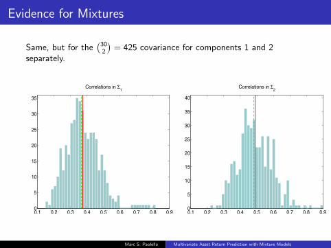
Evidence for Mixtures
Same, but for the d = 30 variances for components 1 and 2 separately.
0 1 2 3 4 50
1
2
3
4
5
6
7
Variances in Σ1
0 10 20 30 40 50 600
1
2
3
4
5
6
7
8
Variances in Σ2
Marc S. Paolella Multivariate Asset Return Prediction with Mixture Models
Evidence for Mixtures
Same, but for the(302
)= 425 covariance for components 1 and 2
separately.
0.1 0.2 0.3 0.4 0.5 0.6 0.7 0.8 0.90
5
10
15
20
25
30
35
Correlations in Σ1
0.1 0.2 0.3 0.4 0.5 0.6 0.7 0.8 0.90
5
10
15
20
25
30
35
40
Correlations in Σ2
Marc S. Paolella Multivariate Asset Return Prediction with Mixture Models

Shrinkage Estimation
Shrinkage estimation is crucial in this context for both numeric reasons,and (far) improved estimation.
The paper gives full details on how this is done.
Our shrinkage prior, as a function of the scalar hyper-parameter ω, is
a1 = 2ω, a2 = ω/2, c1 = c2 = 20ω, m1 = 0p, m2 = (−0.1)1p,
B1 = a1[(1.5− 0.6)Ip + 0.6Jp
], B2 = a2
[(10− 4.6)Ip + 4.6Jp
].
(1)
The only tuning parameter which remains to be chosen is ω.
The effect of different choices of ω is easily and informativelydemonstrated with a simulation study, using the Mix2N30 model, withparameters given by the MLE of the 30 return series.
Marc S. Paolella Multivariate Asset Return Prediction with Mixture Models
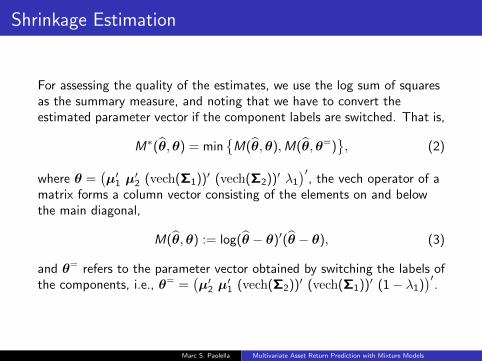
Shrinkage Estimation
For assessing the quality of the estimates, we use the log sum of squaresas the summary measure, and noting that we have to convert theestimated parameter vector if the component labels are switched. That is,
M∗(θ,θ) = min{
M(θ,θ),M(θ,θ=)}, (2)
where θ =(µ′1 µ
′2 (vech(Σ1))′ (vech(Σ2))′ λ1
)′, the vech operator of a
matrix forms a column vector consisting of the elements on and belowthe main diagonal,
M(θ,θ) := log(θ − θ)′(θ − θ), (3)
and θ= refers to the parameter vector obtained by switching the labels ofthe components, i.e., θ= =
(µ′2 µ
′1 (vech(Σ2))′ (vech(Σ1))′ (1− λ1)
)′.
Marc S. Paolella Multivariate Asset Return Prediction with Mixture Models
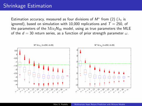
Shrinkage Estimation
Estimation accuracy, measured as four divisions of M∗ from (2) (λ1 isignored), based on simulation with 10,000 replications and T = 250, ofthe parameters of the Mix2N30 model, using as true parameters the MLEof the d = 30 return series, as a function of prior strength parameter ω.
−4
−3.5
−3
−2.5
−2
−1.5
−1
−0.5
0
0.5
ω =0ω =
4ω =
8
ω =12
ω =16
ω =20
ω =24
ω =28
ω =32
ω =36
ω =∞
M* for μ1 (n=250, d=30)
−2
−1
0
1
2
3
4
ω =0ω =
4ω =
8
ω =12
ω =16
ω =20
ω =24
ω =28
ω =32
ω =36
ω =∞
M* for μ2 (n=250, d=30)
Marc S. Paolella Multivariate Asset Return Prediction with Mixture Models

Shrinkage Estimation
1.5
2
2.5
3
3.5
4
ω =0ω =
4ω =
8
ω =12
ω =16
ω =20
ω =24
ω =28
ω =32
ω =36
ω =∞
M* for (vech of) Σ1 (n=250, d=30)
6
6.5
7
7.5
8
8.5
9
9.5
10
ω =0ω =
4ω =
8
ω =12
ω =16
ω =20
ω =24
ω =28
ω =32
ω =36
ω =∞
M* for (vech of) Σ2 (n=250, d=30)
Marc S. Paolella Multivariate Asset Return Prediction with Mixture Models

Component Separation
The Ht,j are the posterior probabilities from the EM algorithm thatobservation Yt came from component j , t = 1, . . . ,T , j = 1, 2,conditional on all the Yt and the estimated components.
It is natural to plot these versus time.
0 500 1000 1500
0
0.1
0.2
0.3
0.4
0.5
0.6
0.7
0.8
0.9
1
Final values of Ht1
versus t=1...1945
0 50 100 150 200 250
0
0.1
0.2
0.3
0.4
0.5
0.6
0.7
0.8
0.9
1
Final values of Ht1
for last 250 values
One might be tempted to use this finding as further evidence for theclaim that there exist two, reasonably distinct, ’regimes’ in financialmarkets, but this is not the case!
The same effect would occur if the data had arisen from a fat-tailedsingle-component multivariate distribution.
Marc S. Paolella Multivariate Asset Return Prediction with Mixture Models

Component Separation
Now use a multivariate normal distribution (left) and a heavier-tailedmultivariate Laplace, both of which are single-component densities!Then fit fit the 2-comp mixture of normals.
0 500 1000 1500 20000
0.1
0.2
0.3
0.4
0.5
0.6
0.7
0.8
0.9
1
0 500 1000 1500 20000
0.1
0.2
0.3
0.4
0.5
0.6
0.7
0.8
0.9
1
Thus, the separation apparent for the DJ-30 data is necessary, but clearlynot sufficient to declare that the data were generated by a mixturedistribution.
Stronger evidence for mixtures comes from the earlier graphic: themeans of the first and second component differ markedly, with the latterbeing primarily negative, and the correlations in the second componentare on average higher than those associated with component 1.
Marc S. Paolella Multivariate Asset Return Prediction with Mixture Models
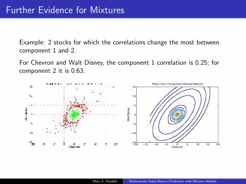
Further Evidence for Mixtures
Example: 2 stocks for which the correlations change the most betweencomponent 1 and 2.
For Chevron and Walt Disney, the component 1 correlation is 0.25; forcomponent 2 it is 0.63.
Fitted Two−Component Normal Mixture
Chevron
Wal
t Dis
ney
−20 −15 −10 −5 0 5 10 15 20−15
−10
−5
0
5
10
15
Marc S. Paolella Multivariate Asset Return Prediction with Mixture Models

Component Inspection: Is Normality Adequate?
The apparent separation is highly advantageous because it allows us toassign each Yt to one of the two components with very high confidence.
Once done, we can assess how well each of the two estimated multivariatenormal distributions fits the observations assigned to its component.
We use the criteria Ht,1 > 0.99, choosing to place those Yt whosecorresponding values of Ht,1 suggest even a slight influence fromcomponent 2, into this more volatile component.
This results in 1,373 observations assigned to component 1, or 70.6% ofthe observations, and 572 to the second component.
Marc S. Paolella Multivariate Asset Return Prediction with Mixture Models

Component Inspection: Is Normality Adequate?
Based on the split, for each of the k × d = 60 series, we fit a flexible,asymmetric, fat-tailed distribution.We use the generalized asymmetric t, or GAt, distribution, withlocation-zero, scale-one pdf given by (p, ν, θ ∈ R>0)
fGAt (z ; p, ν, θ) = Cp,ν,θ ×
(1 +
(−z · θ)p
ν
)−(ν+ 1p ), if z < 0,
(1 +
(z/θ)p
ν
)−(ν+ 1p ), if z ≥ 0,
Parameter p measures the peakedness of the density, with values nearone indicative of Laplace-type behavior, while values near two indicate apeak similar to that of the Gaussian and Student’s t distributions.
Parameter v indicates the tail thickness, and is analogous to the degreesof freedom parameter.
Parameter θ, controls the asymmetry, with values less than 1 indicatingnegative skewness.
Marc S. Paolella Multivariate Asset Return Prediction with Mixture Models

Component Inspection: Is Normality Adequate?
Remember: Parameter v indicates the tail thickness analogous to the dfin the Student’t t, except that moments of order v · p and higher do notexist. So that, if p = 2, then we would double the value of v to make itcomparable to the df in the usual Student’s t.
−1
0
1
2
3
4
5
6
7
8Component 1 (EM 0.99)
p v θ μ c Sk−1
0
1
2
3
4
5
6
7
8Component 2 (EM 0.99)
p v θ μ c Sk
Marc S. Paolella Multivariate Asset Return Prediction with Mixture Models

Worst Case: McDonalds
−6 −4 −2 0 2 4 60
0.05
0.1
0.15
0.2
0.25
0.3
0.35
0.4McDonald’s Component 1 Fitted Densities
Uncon: pML
=2.4 vML
=2.0
Const: pML
=1.4 vML
=90
−10 −5 0 5 100
0.05
0.1
0.15
0.2
0.25McDonald’s Component 2 Fitted Densities
Uncon: pML
=2.1 vML
=2.1
Const: pML
=1.2 vML
=90
−6 −4 −2 0 2 4 60
0.05
0.1
0.15
0.2
0.25
0.3
0.35
0.4McDonald’s Component 1 Fitted Densities (7 Outliers Removed)
Uncon: pML
=2.0 vML
=5.0
Const: pML
=1.6 vML
=90
−10 −5 0 5 100
0.05
0.1
0.15
0.2
0.25McDonald’s Component 2 Fitted Densities (1 Outlier Removed)
Uncon: pML
=1.9 vML
=2.9
Const: pML
=1.3 vML
=90
Marc S. Paolella Multivariate Asset Return Prediction with Mixture Models

Component Inspection: Is Normality Adequate?
For each of the 30 series, but not separating them into the twocomponents, we fit the GAt, with no parameter restrictions, and with therestriction that 90 < v < 100 (forces normality if p = 2 and θ = 1, orLaplace if p = 1 and θ = 1)
Compute the asymptotically valid p-value of the likelihood ratio test. Ifthat value is less than 0.05, then we remove the largest value (in absoluteterms) from the series, and re-compute the estimates and the p-value.This is repeated until the p-value exceeds 0.05.
We report the smallest number of observations required to be removed inorder to achieve this.
Do this for the actual 30 series, and also the two separated components.
Marc S. Paolella Multivariate Asset Return Prediction with Mixture Models

Component Inspection: Is Normality Adequate?
Stock number 5 is Bank of America, and shows that 65 most extremevalues had to be removed from the series to get the p-value above 0.05,but no observations from component 1 needed to be removed, and only3 from component 2.
Stock # 1 2 3 4 5 6 7 8 9 10 11 12 13 14 15All 19 19 5 2 65 21 11 27 60 10 30 19 28 31 8Comp1 0 0 0 0 0 3 0 0 1 1 1 0 0 0 0Comp2 0 1 0 0 3 1 1 6 8 2 0 8 0 1 1
Stock # 16 17 18 19 20 21 22 23 24 25 26 27 28 29 30All 7 12 8 5 19 7 15 28 3 14 10 11 6 8 10Comp1 0 0 2 2 0 0 7 0 0 0 0 0 0 0 0Comp2 0 0 0 1 0 0 1 2 0 2 1 3 0 2 1
Marc S. Paolella Multivariate Asset Return Prediction with Mixture Models
Density Forecasting
We forecast the entire multivariate density.
The measure of interest is what we will call the (realized)predictive log-likelihood, given by
πt(M, v) = log fMt|It−1(yt ; ψ), (4)
where v denotes the size of the rolling window used to determineIt−1 (and the set of observations used for estimation of ψ) for eachtime point t.
Marc S. Paolella Multivariate Asset Return Prediction with Mixture Models
Density Forecasting
We suggest to use what we refer to as the normalized sum of therealized predictive log-likelihood, given by
Sτ0,T (M, v) =1
(T − τ0) d
T∑
t=τ0+1
πt(M, v), (5)
where d is the dimension of the data.
It is thus the average realized predictive log-likelihood, averaged overthe number of time points used and the dimension of the randomvariable under study. This facilitates comparison over different d , τ0and T .
In our setting, we use the d = 30 daily return series of the DJ-30,with v = τ0 = 500, which corresponds to two years of data, andT = 1, 945.
Marc S. Paolella Multivariate Asset Return Prediction with Mixture Models

Density Forecasting
We compute for set of models indexed by ω, πt(Mω, v) from (4).
We take{Mω
}to be the Mix2N30 model estimated with shrinkage prior
(1) for a given value of hyper-parameter ω.
We do this using a moving window of size v = 250, starting atobservation τ0 = v = 250, and updating parameter vector θ at each timeincrement.
Marc S. Paolella Multivariate Asset Return Prediction with Mixture Models

Density Forecasting: Finding the optimal ω
0 200 400 600 800 1000 1200 1400 16000
1000
2000
3000
4000
5000
6000
Normalized Cusum C(h,ω)−C(h,0.1)
h−τ0+1 for τ
0=250
ω=25ω=20ω=15ω=10ω=5
0 20 40 60 80 100−1.76
−1.74
−1.72
−1.7
−1.68
−1.66
−1.64
−1.62S250,1945(Mω, v)
Prior Strength ω
rolling window, v=250rolling window, v=1000
Here,
C (h, ω) =h∑
t=τ0+1
πt(Mω, 250), h = τ0 + 1, . . . ,T ,
Marc S. Paolella Multivariate Asset Return Prediction with Mixture Models

Optimal Shrinkage as a Function of d
5 10 15 20 25 30
5
10
15
20
25
30
35
40
45
50
ω*(250)
5 10 15 20 25 30−2.05
−2
−1.95
−1.9
−1.85
−1.8
−1.75
−1.7
−1.65
−1.6
−1.55S250,1945(Mω∗(250), 250)
5 10 15 20 25 30−2.05
−2
−1.95
−1.9
−1.85
−1.8
−1.75
−1.7
−1.65
−1.6
−1.55S250,1945(Mω, 250)
ω = ω∗(250) (original graphic)ω = ωreg(250)
5 10 15 20 25 30−2.05
−2
−1.95
−1.9
−1.85
−1.8
−1.75
−1.7
−1.65
−1.6
−1.55S250,1945(Mω, 250)
ω = ω∗(250) (original graphic)ω = 1
Marc S. Paolella Multivariate Asset Return Prediction with Mixture Models
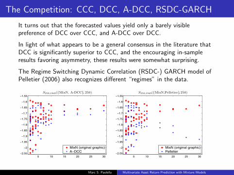
The Competition: CCC, DCC, A-DCC, RSDC-GARCH
It turns out that the forecasted values yield only a barely visiblepreference of DCC over CCC, and A-DCC over DCC.
In light of what appears to be a general consensus in the literature thatDCC is significantly superior to CCC, and the encouraging in-sampleresults favoring asymmetry, these results were somewhat surprising.
The Regime Switching Dynamic Correlation (RSDC-) GARCH model ofPelletier (2006) also recognizes different “regimes” in the data.
5 10 15 20 25 30−2.05
−2
−1.95
−1.9
−1.85
−1.8
−1.75
−1.7
−1.65
−1.6
−1.55S250,1945({MixN, A-DCC}, 250)
MixN (original graphic)A−DCC
5 10 15 20 25 30−2.05
−2
−1.95
−1.9
−1.85
−1.8
−1.75
−1.7
−1.65
−1.6
−1.55S250,1945({MixN,Pelletier}, 250)
MixN (original graphic)Pelletier
Marc S. Paolella Multivariate Asset Return Prediction with Mixture Models
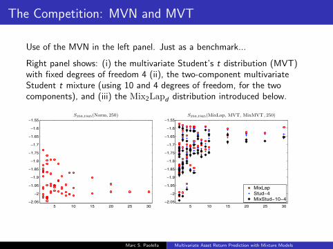
The Competition: MVN and MVT
Use of the MVN in the left panel. Just as a benchmark...
Right panel shows: (i) the multivariate Student’s t distribution (MVT)with fixed degrees of freedom 4 (ii), the two-component multivariateStudent t mixture (using 10 and 4 degrees of freedom, for the twocomponents), and (iii) the Mix2Lapd distribution introduced below.
5 10 15 20 25 30−2.05
−2
−1.95
−1.9
−1.85
−1.8
−1.75
−1.7
−1.65
−1.6
−1.55S250,1945(Norm, 250)
5 10 15 20 25 30−2.05
−2
−1.95
−1.9
−1.85
−1.8
−1.75
−1.7
−1.65
−1.6
−1.55S250,1945(MixLap, MVT, MixMVT , 250)
MixLapStud−4MixStud−10−4
Marc S. Paolella Multivariate Asset Return Prediction with Mixture Models

Why does Mix2Lapd beat Mix2Studd
From a forecasting point of view, the Laplace mixture resulted in superiorperformance. We conjecture the reason for this to be that the tails of thet, when used in a mixture context, are too fat.
While higher kurtosis is indeed still required for the second component,the Laplace offers this without power tails and the ensuing upper boundon finite absolute positive moments.
Moreover, as demonstrated above via use of the GAt distribution and thefitted values of peakedness parameter p, there is evidence that the twocomponents, particularly the second, have a more peaked distributionthan the Student’s t.
Marc S. Paolella Multivariate Asset Return Prediction with Mixture Models
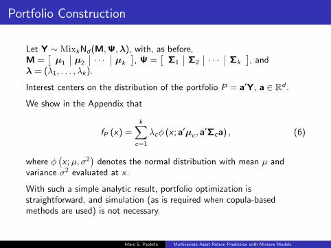
Portfolio Construction
Let Y ∼ MixkNd(M,Ψ,λ), with, as before,M =
[µ1 µ2 · · · µk
], Ψ =
[Σ1 Σ2 · · · Σk
], and
λ = (λ1, . . . , λk).
Interest centers on the distribution of the portfolio P = a′Y, a ∈ Rd .
We show in the Appendix that
fP (x) =k∑
c=1
λcφ (x ; a′µc , a′Σca) , (6)
where φ(x ;µ, σ2
)denotes the normal distribution with mean µ and
variance σ2 evaluated at x .
With such a simple analytic result, portfolio optimization isstraightforward, and simulation (as is required when copula-basedmethods are used) is not necessary.
Marc S. Paolella Multivariate Asset Return Prediction with Mixture Models

Portfolio Construction
With µc = a′µc and σ2c = a′Σca, c = 1, . . . , k ,
µP = E [P] =k∑
c=1
λcµc , σ2P = V (P) =
k∑
c=1
λc(σ2c + µ2
c
)− µ2
P .
It is common when working with non-Gaussian portfolio distributions touse a measure of downside risk, such as the value-at-risk (VaR), or theexpected shortfall (ES).
Marc S. Paolella Multivariate Asset Return Prediction with Mixture Models

Portfolio Construction
The VaR involves the γ-quantile of P, denoted qP,γ , for 0 < γ < 1, withγ typically 0.01 or 0.05, and which can be found numerically by using thecdf of P, easily seen to be FP (x) =
∑kc=1 λcΦ ((x − µc)/σc), with Φ the
standard normal cdf.
The γ-level ES of P is given by
ESγ (P) =1
γ
∫ γ
0
QP (p) dp,
where QP is the quantile function of P. We prove in the Appendix thatthis integral can be represented analytically as
ESγ (P) =k∑
j=1
λjΦ (cj)
γ
{µj − σj
φ (cj)
Φ (cj)
}, cj =
qP,γ − µj
σj, qP,γ = QP (γ) .
Marc S. Paolella Multivariate Asset Return Prediction with Mixture Models

Multivariate Laplace
The d-variate multivariate Laplace distribution is given by
fY (y,µ,Σ, b) =1
|Σ|1/2 (2π)d/22
Γ (b)
(m
2
)b/2−d/4Kb−d/2
(√2m), (7)
where m = (y − µ)′Σ−1(y − µ).
It generalizes several constructs in the literature, but itself is a specialcase of the multivariate generalized hyperbolic distribution.
We write Y ∼ Lap (µ,Σ, b).
Marc S. Paolella Multivariate Asset Return Prediction with Mixture Models
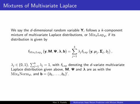
Mixtures of Multivariate Laplace
We say the d-dimensional random variable Yi follows a k-componentmixture of multivariate Laplace distributions, or MixkLapd , if itsdistribution is given by
fMixkLapd(y; M,Ψ,λ,b) =
k∑
j=1
λj fLap(y;µj ,Σj , bj
),
λj ∈ (0, 1),∑k
j=1 λj = 1, with fLap denoting the d-variate multivariateLaplace distribution given above, M, Ψ and λ are as with theMixkNormd , and b = (b1, . . . , bk)′.
Marc S. Paolella Multivariate Asset Return Prediction with Mixture Models

Mixtures of Multivariate Laplace
We observe d-variate random variables Yt = (Yt,1,Yt,2, . . . ,Yt,d)′,
t = 1, . . . ,T , with Yti.i.d.∼ MixkLapd(M,Ψ,λ,b), and take the values of
b = (b1, . . . , bk) to be known constants.
Interest centers on estimation of the remaining parameters.
This is conducted via an EM algorithm, the derivation of which is givenin the Appendix.
In addition, the EM recursions are extended there to support use of aquasi-Bayesian paradigm analogous to that used for the MixkNd
distribution.
Marc S. Paolella Multivariate Asset Return Prediction with Mixture Models

Estimation of the bi in the Mixture of Multivariate Laplace
We use the profile likelihood to each component, applied to the split datavia the EM algorithm.
The details are in the paper. This is not optimal, but adequate.
1 3 5 7 9 11 13 15−5.47
−5.46
−5.45
−5.44
−5.43
−5.42
−5.41Component 1 Log lik (ω=50) Using EM Split
MVL parameter b
log
likel
ihoo
d / 1
0000
1 3 5 7 9 11 13 15−4.035
−4.03
−4.025
−4.02
−4.015Component 2 Log lik (ω=50) Using EM Split
MVL parameter b
log
likel
ihoo
d / 1
0000
Marc S. Paolella Multivariate Asset Return Prediction with Mixture Models
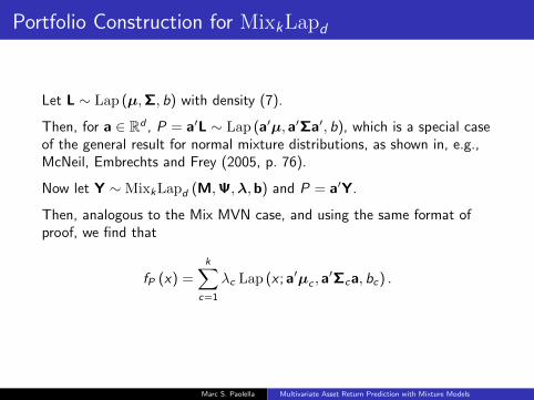
Portfolio Construction for MixkLapd
Let L ∼ Lap (µ,Σ, b) with density (7).
Then, for a ∈ Rd , P = a′L ∼ Lap (a′µ, a′Σa′, b), which is a special caseof the general result for normal mixture distributions, as shown in, e.g.,McNeil, Embrechts and Frey (2005, p. 76).
Now let Y ∼ MixkLapd (M,Ψ,λ,b) and P = a′Y.
Then, analogous to the Mix MVN case, and using the same format ofproof, we find that
fP (x) =k∑
c=1
λc Lap (x ; a′µc , a′Σca, bc) .
Marc S. Paolella Multivariate Asset Return Prediction with Mixture Models

Portfolio Construction for MixkLapd
Similar to (33), we have, with µc = a′µc and σ2c = a′Σca, c = 1, . . . , k,
µP = E [P] =k∑
c=1
λcµc , σ2P = V (P) =
k∑
c=1
λc(bcσ
2c + µ2
c
)− µ2
P .
A closed-form expression for the expected shortfall is currently notavailable.
Though given the tractable density function of P, and the exponential(not power) tails of the Laplace distribution, numeric integration tocompute the relevant quantile, and the integral associated with theexpected shortfall, will be fast and reliable.
Marc S. Paolella Multivariate Asset Return Prediction with Mixture Models