multivariate longitudinal data analysis for actuarial...
TRANSCRIPT
Multivariate longitudinal data analysis foractuarial applications
Priyantha Kumara and Emiliano A. Valdez
astin/afir/iaals Mexico Colloquia 2012
Mexico City, Mexico, 1-4 October 2012
P. Kumara and E.A. Valdez, U of Connecticut Multivariate longitudinal data analysis 1/28

Outline
IntroductionSome literature
The model specificationNotationKey features of our approachMultivariate joint distributionChoice for the marginals: the class of GB2
Case studyGlobal insurance demand
Additional work intended
Selected reference
P. Kumara and E.A. Valdez, U of Connecticut Multivariate longitudinal data analysis 2/28
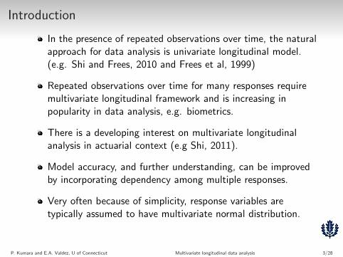
Introduction
In the presence of repeated observations over time, the naturalapproach for data analysis is univariate longitudinal model.(e.g. Shi and Frees, 2010 and Frees et al, 1999)
Repeated observations over time for many responses requiremultivariate longitudinal framework and is increasing inpopularity in data analysis, e.g. biometrics.
There is a developing interest on multivariate longitudinalanalysis in actuarial context (e.g Shi, 2011).
Model accuracy, and further understanding, can be improvedby incorporating dependency among multiple responses.
Very often because of simplicity, response variables aretypically assumed to have multivariate normal distribution.
P. Kumara and E.A. Valdez, U of Connecticut Multivariate longitudinal data analysis 3/28
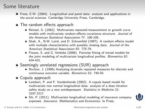
Some literatureFrees, E.W. (2004). Longitudinal and panel data: analysis and applications inthe social sciences. Cambridge University Press, Cambridge.
The random effects approachReinsel, G. (1982). Multivariate repeated-measurement or growth curvemodels with multivariate random-effects covariance structure. Journal ofthe American Statistical Association 77: 190-195.Shah, A., N.M. Laird, and D. Schoenfeld (1997). A random effects modelwith multiple characteristics with possibly missing data. Journal of theAmerican Statistical Association 92: 775-79.Fieuws, S. and G. Verbeke (2006). Pairwise fitting of mixed models forthe joint modeling of multivariate longitudinal profiles. Biometrics 62:424-431.
Seemingly unrelated regressions (SUR) approachRochon, J. (1996) Analyzing bivariate repeated measures for discrete andcontinuous outcome variable. Biometrics 52: 740-50.
Copula approachLambert, P. and F. Vandenhende (2002). A copula based model formultivariate non normal longitudinal data: analysis of a dose titrationsafety study on a new antidepressant. Statistics in Medicine 21:3197-3217.Shi, P. (2011). Multivariate longitudinal modeling of insurance companyexpenses. Insurance: Mathematics and Economics. In Press.
P. Kumara and E.A. Valdez, U of Connecticut Multivariate longitudinal data analysis 4/28
Our contribution
Methodology
We propose the use of a random effects model to capturedynamic dependency and heterogeneity, and a copula functionto incorporate dependency among the response variables.
Multivariate longitudinal analysis for actuarial applications
We intend to explore actuarial-related problems withinmultivariate longitudinal context, and apply our proposedmethodology.
NOTE: Our results are very preliminary at this stage.
P. Kumara and E.A. Valdez, U of Connecticut Multivariate longitudinal data analysis 5/28

Notation
Suppose we have a set of q covariates associated with n subjectscollected over T time periods for a set of m response variables.
Let yit,k denote the responses from ith individual in tth time periodon the kth response. By letting yit = (yit,1, yit,2, . . . , yit,m)′ fort = 1, 2, . . . , T , we can express Yi = (yi1,yi2, . . . ,yiT).
Covariates associated with the ith subject in tth time period on thekth response can be expressed as xit = (xit,1,xit,2, . . . ,xit,m)where xit,k = (xit1,k, xit2,k, . . . , xitp,k) for k = 1, 2, ...m.
We use αik to represent the random effects componentcorresponding to the ith subject from the kth response variable.
G (αik) represents the pre-specified distribution function of randomeffect αik.
P. Kumara and E.A. Valdez, U of Connecticut Multivariate longitudinal data analysis 6/28

Key features of our approach
Obviously, the extension from univariate to multivariatelongitudinal analysis.
Types of dependencies captured:the dependence structure of the response using copulas -provides flexibility
the intertemporal dependence within subjects andunobservable subject-specific heterogeneity captured throughthe random effects component - provides tractability
The marginal distribution models:any family of flexible enough distributions can be used
choose family so that covariate information can be easilyincorporated
Other key features worth noting:the parametric model specification provides flexibility forinference e.g. MLE for estimation
model construction can accommodate both balanced andunbalanced data - an important feature for longitudinal data
P. Kumara and E.A. Valdez, U of Connecticut Multivariate longitudinal data analysis 7/28

Copula function
For arbitrary m uniform random variables on the unit interval,copula function, C, can be uniquely defined as
C(u1, . . . , um) = P (U1 ≤ u1, . . . , Um ≤ um).
Joint distribution:
F (y1, . . . , ym) = C(F1(y1), . . . , Fm(ym)),
where Fk(yk) are marginal distribution functions.
Joint density:
f(y1, . . . , ym) = c(F1(y1), ..., Fm(ym))
m∏k=1
fk(yk),
where fk(yk) are marginal density functions and c is thedensity associated with copula C.
P. Kumara and E.A. Valdez, U of Connecticut Multivariate longitudinal data analysis 8/28
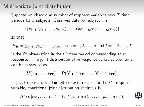
Multivariate joint distribution
Suppose we observe m number of response variables over T timeperiods for n subjects. Observed data for subject i is
{(yi1,1, yi1,2, . . . , yi1,m), . . . , (yiT,1, yiT,2, . . . , yiT,m)}
so that
Yit = (yit,1, yit,2, . . . , yit,m) for i = 1, 2, . . . , n and t = 1, 2, . . . , T
is the ith observation in the tth time period corresponding to mresponses. The joint distribution of m response variables over timecan be expressed as
H(yi1, . . . ,yiT) = P(Yi1 ≤ yi1, . . . ,YiT ≤ yiT).
If {αik} represent random effects with respect to the kth responsevariable, conditional joint distribution at time t is
H(yit|αi1, . . . , αim) = C(F (yit,1|αi1), . . . , F (yit,m|αim)).
P. Kumara and E.A. Valdez, U of Connecticut Multivariate longitudinal data analysis 9/28

- continued
Conditional joint density at time t:
h(yit|αi1, . . . , αim) = c(F (yit,1|αi1), . . . , F (yit,m|αim))
m∏k=1
f(yit,k|αik)
where F (yit,k|αik) denotes the distribution function of kth
response variable at time t. If ω represents the set of parameters inthe model, the likelihood of the ith subject is given by
L(ω|(yi1, . . . ,yiT)) = h(yi1, . . . ,yiT|ω).
We can write
h(yi1, . . . ,yiT|ω) =
∫αi1
. . .
∫αim
h(yi1, . . . ,yiT|αi1, . . . , αim)
dG (αi1) · · · dG (αim)
Under independence over time for a given random effect:
h(yi1, . . . ,yiT|αi1, . . . , αim) =T∏t=1
h(yit|αi1, . . . , αim)P. Kumara and E.A. Valdez, U of Connecticut Multivariate longitudinal data analysis 10/28

- continued
=
∫αi1
. . .
∫αim
T∏t=1
h(yit|αi1, . . . , αim)dG (αi1) · · · dG (αim)
and from the previous slides, we have
=
∫αi1
. . .
∫αim
T∏t=1
c(F (yit,1|αi1), . . . , F (yit,m|αim))
m∏k=1
f(yit,k|αik)dG (αi1) · · · dG (αim)
Then, we can write the log likelihood function as
∑i
log{∫
αi1
. . .
∫αim
T∏t=1
m∏k=1
c(F (yit,1|α1), . . . , F (yit,m|αm))
× f(yit,k|αik)dG (αi1) · · · dG (αim)}
P. Kumara and E.A. Valdez, U of Connecticut Multivariate longitudinal data analysis 11/28

Choice for the marginals: the class of GB2
The model specification is flexible enough to accommodate anymarginals; however, for our purposes, we chose the class of GB2distributions. For Y ∼ GB2(a, b, p, q) with a 6= 0, b, p, q > 0:
Density function:
fy(y) =|a| yap−1baq
B(p, q)(ba + ya)(p+q)
where B (·, ·) is the usual Beta function.
Distribution function:
Fy(y) = B
((y/b)a
1 + (y/b)a; p, q
)where B (·; ·, ·) is the incomplete Beta function.
Mean:
E(Y ) = bB (p+ 1/a, q − 1/a)
B(p, q).
P. Kumara and E.A. Valdez, U of Connecticut Multivariate longitudinal data analysis 12/28
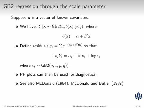
GB2 regression through the scale parameter
Suppose x is a vector of known covariates:
We have: Y |x ∼ GB2(a, b(x), p, q), where
b(x) = α+ β′x
Define residuals εi = Yie−(αi+β
′xi) so that
log Yi = αi + β′xi + log εi
where εi ∼ GB2(a, 1, p, q)).
PP plots can then be used for diagnostics.
See also McDonald (1984), McDonald and Butler (1987)
P. Kumara and E.A. Valdez, U of Connecticut Multivariate longitudinal data analysis 13/28
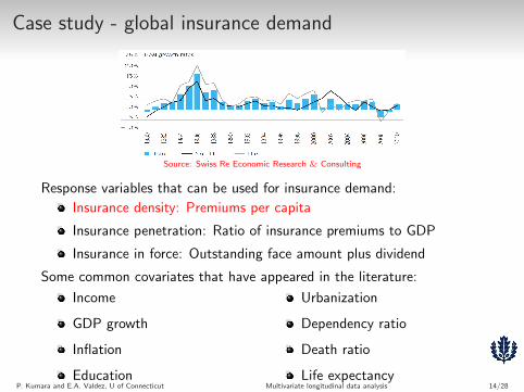
Case study - global insurance demand
Source: Swiss Re Economic Research & Consulting
Response variables that can be used for insurance demand:
Insurance density: Premiums per capita
Insurance penetration: Ratio of insurance premiums to GDP
Insurance in force: Outstanding face amount plus dividend
Some common covariates that have appeared in the literature:
Income
GDP growth
Inflation
Education
Urbanization
Dependency ratio
Death ratio
Life expectancyP. Kumara and E.A. Valdez, U of Connecticut Multivariate longitudinal data analysis 14/28

About the data set
Data set
2 responses: life and non-life insurance
5 predictor variables
75 countries (originally, later removed 3 countries)
6 years data (from year 2004 to year 2009)
Variables in the model
Dependent variables
Non-life density Premiums per capita in non-life insurance
Life density Premiums per capita in life insurance
Independent variables
GDP per capita Ratio of gross domestic product (current US dollars) to total population
Religious Percentage of Muslim population
Urbanization Percentage of urban population to total population
Death rate Percentage of death
Dependency ratio Ratio of population over 65 to working population
Sources: Swiss Re sigma reports through the Insurance Information Institute (III); World Bank
P. Kumara and E.A. Valdez, U of Connecticut Multivariate longitudinal data analysis 15/28

Multiple time series plot
Non-life insurance
Year
Pre
miu
ms
per c
apita
2004 2005 2006 2007 2008 2009
01000
2000
3000
4000
Netherland
Switzerland
IrelandUSA
Life insurance
Year
Pre
miu
ms
per c
apita
2004 2005 2006 2007 2008 20090
2000
4000
6000
8000
10000 Ireland
UK
USA
P. Kumara and E.A. Valdez, U of Connecticut Multivariate longitudinal data analysis 16/28
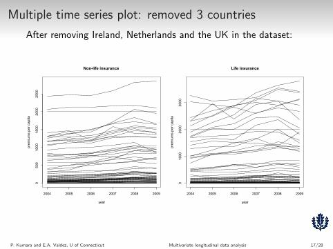
Multiple time series plot: removed 3 countries
After removing Ireland, Netherlands and the UK in the dataset:
Non-life insurance
year
prem
ium
s pe
r cap
ita
2004 2005 2006 2007 2008 2009
0500
1000
1500
2000
2500
Life insurance
year
prem
ium
s pe
r cap
ita
2004 2005 2006 2007 2008 2009
01000
2000
3000
P. Kumara and E.A. Valdez, U of Connecticut Multivariate longitudinal data analysis 17/28
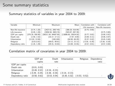
Some summary statistics
Summary statistics of variables in year 2004 to 2009:
Variable Minimum Maximum Mean Correlation with Correlation withLife insurance Non-life insurance
Non-life insurance (0.74, 1.26) (2427.61, 2857.40) (386.28, 516.99) (0.75, 0.80) -Life insurance (0.49, 1.28) (3058.58, 3803.76) (503.87, 697.39) - (0.75, 0.80)GDP per capita (375.20, 550.90) (56311.50, 94567.90) (13896.60, 20524.50) (0.77, 0.82) (0.90, 0.91)Death rate (1.50, 1.52) (16.17, 17.11) (7.87, 8.00) (0.09, 0.11) (0.06, 0.07)Urbanization (11.92, 13.56) (100,100) (64.90, 66.29) (0.37, 0.42) (0.45, 0.46)Religious (0.01,0.01) (99.61, 99.61) (22.12, 22.12) (-0.30, -0.29) (-0.30, -0.28)Dependency ratio (1.25, 1.39) (29.31, 33.92) (14.89, 15.55) (0.57, 0.61) (0.57, 0.60)
Correlation matrix of covariates in year 2004 to 2009:
GDP per Death Urbanization Religious Dependencycapita rate ratio
GDP per capita -Death rate (0.01, 0.03) -Urbanization (0.49, 0.52) (-0.16, -0.15) -Religious (-0.29, -0.25) (-0.38, -0.34) (-0.14, -0.13) -Dependency ratio (0.58, 0.62) (0.53, 0.54) (0.30, 0.32) (-0.53, -0.52) -
P. Kumara and E.A. Valdez, U of Connecticut Multivariate longitudinal data analysis 18/28

Scatter plots of the two response variables
Year 2004
Pearson correlation: 0.80
0 500 1000 1500 2000 2500
01000
2000
3000
Year 2005
Pearson correlation: 0.78
0 500 1000 1500 2000 2500
01000
2000
3000
Year 2006
Pearson correlation: 0.77
0 500 1000 1500 2000 2500
01000
2000
3000
Year 2007
Pearson correlation: 0.75
0 500 1000 1500 2000 2500
01000
2000
3000
Year 2008
Pearson correlation: 0.78
0 500 1000 1500 2000 2500
01000
2000
3000
Year 2009
Pearson correlation: 0.74
0 500 1000 1500 2000 2500
01000
2000
3000
x-axis: non-life insurance and y-axis: life insuranceP. Kumara and E.A. Valdez, U of Connecticut Multivariate longitudinal data analysis 19/28
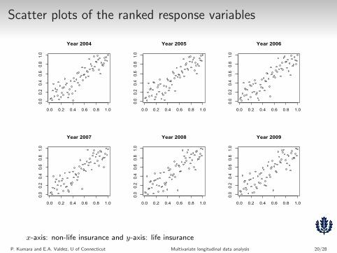
Scatter plots of the ranked response variables
0.0 0.2 0.4 0.6 0.8 1.0
0.0
0.2
0.4
0.6
0.8
1.0
Year 2004
0.0 0.2 0.4 0.6 0.8 1.0
0.0
0.2
0.4
0.6
0.8
1.0
Year 2005
0.0 0.2 0.4 0.6 0.8 1.0
0.0
0.2
0.4
0.6
0.8
1.0
Year 2006
0.0 0.2 0.4 0.6 0.8 1.0
0.0
0.2
0.4
0.6
0.8
1.0
Year 2007
0.0 0.2 0.4 0.6 0.8 1.0
0.0
0.2
0.4
0.6
0.8
1.0
Year 2008
0.0 0.2 0.4 0.6 0.8 1.0
0.0
0.2
0.4
0.6
0.8
1.0
Year 2009
x-axis: non-life insurance and y-axis: life insurance
P. Kumara and E.A. Valdez, U of Connecticut Multivariate longitudinal data analysis 20/28
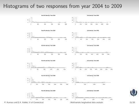
Histograms of two responses from year 2004 to 2009
Non-life density: Year 2004
0 500 1000 1500 2000 2500
020
Life density: Year 2004
0 500 1000 1500 2000 2500 3000
020
40
Non-life density: Year 2005
0 500 1000 1500 2000 2500
015
30
Life density: Year 2005
0 500 1000 1500 2000 2500 3000
020
40
Non-life density: Year 2006
0 500 1000 1500 2000 2500
010
25
Life density: Year 2006
0 500 1000 1500 2000 2500 3000
020
40
Non-life density: Year 2007
0 500 1000 1500 2000 2500
010
25
Life density: Year 2007
0 500 1000 1500 2000 2500 3000 3500
015
30
Non-life density: Year 2008
0 500 1000 1500 2000 2500 3000
010
20
Life density: Year 2008
0 1000 2000 3000
015
30
Non-life density: Year 2009
0 500 1000 1500 2000 2500 3000
010
20
Life density: Year 2009
0 1000 2000 3000 4000
015
30
P. Kumara and E.A. Valdez, U of Connecticut Multivariate longitudinal data analysis 21/28

Model calibration
Marginals: GB2 with regression on the scale parameter
Gaussian copula:
C(u1, u2; ρ) = Φρ(Φ−1(u1),Φ
−1(u2))
Natural assumption for random effect for the kth response:
αik ∼ N(0, σ2k
)
P. Kumara and E.A. Valdez, U of Connecticut Multivariate longitudinal data analysis 22/28
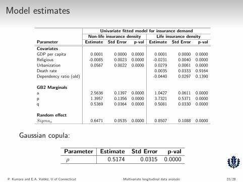
Model estimates
Univariate fitted model for insurance demandNon-life insurance density Life insurance density
Parameter Estimate Std Error p-val Estimate Std Error p-val
CovariatesGDP per capita 0.0001 0.0000 0.0000 0.0001 0.0000 0.0000Religious -0.0085 0.0023 0.0000 -0.0231 0.0040 0.0000Urbanization 0.0567 0.0022 0.0000 0.0279 0.0061 0.0000Death rate 0.0035 0.0333 0.9164Dependency ratio (old) -0.0440 0.0297 0.1390
GB2 Marginalsa 2.5636 0.1397 0.0000 1.0427 0.0611 0.0000p 1.3957 0.1356 0.0000 3.7321 0.5371 0.0000q 0.5369 0.0364 0.0000 0.5081 0.0330 0.0000
Random effectSigmaα 0.6471 0.0535 0.0000 0.8507 0.1088 0.0000
Gaussian copula:
Parameter Estimate Std Error p-valρ 0.5174 0.0315 0.0000
P. Kumara and E.A. Valdez, U of Connecticut Multivariate longitudinal data analysis 23/28

PP plots of the residuals for marginal diagnostics
Non-life Insurance
0.0 0.2 0.4 0.6 0.8 1.0
0.00.20.40.60.81.0
Year 2004
theoretical probability
sam
ple
prob
abilit
y
0.0 0.2 0.4 0.6 0.8 1.0
0.00.20.40.60.81.0
Year 2005
theoretical probability
sam
ple
prob
abilit
y0.0 0.2 0.4 0.6 0.8 1.0
0.00.20.40.60.81.0
Year 2006
theoretical probability
sam
ple
prob
abilit
y0.0 0.2 0.4 0.6 0.8 1.0
0.00.20.40.60.81.0
Year 2007
theoretical probability
sam
ple
prob
abilit
y
0.0 0.2 0.4 0.6 0.8 1.0
0.00.20.40.60.81.0
Year 2008
theoretical probability
sam
ple
prob
abilit
y
0.0 0.2 0.4 0.6 0.8 1.0
0.00.20.40.60.81.0
Year 2009
theoretical probabilitysa
mpl
e pr
obab
ility
P. Kumara and E.A. Valdez, U of Connecticut Multivariate longitudinal data analysis 24/28
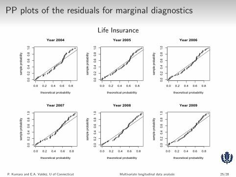
PP plots of the residuals for marginal diagnostics
Life Insurance
0.0 0.2 0.4 0.6 0.8
0.00.20.40.60.81.0
Year 2004
theoretical probability
sam
ple
prob
abilit
y
0.0 0.2 0.4 0.6 0.8
0.00.20.40.60.81.0
Year 2005
theoretical probability
sam
ple
prob
abilit
y0.0 0.2 0.4 0.6 0.8
0.00.20.40.60.81.0
Year 2006
theoretical probability
sam
ple
prob
abilit
y0.0 0.2 0.4 0.6 0.8
0.00.20.40.60.81.0
Year 2007
theoretical probability
sam
ple
prob
abilit
y
0.0 0.2 0.4 0.6 0.8
0.00.20.40.60.81.0
Year 2008
theoretical probability
sam
ple
prob
abilit
y
0.0 0.2 0.4 0.6 0.8
0.00.20.40.60.81.0
Year 2009
theoretical probabilitysa
mpl
e pr
obab
ility
P. Kumara and E.A. Valdez, U of Connecticut Multivariate longitudinal data analysis 25/28
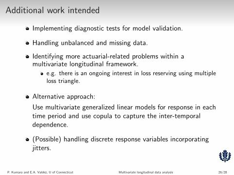
Additional work intended
Implementing diagnostic tests for model validation.
Handling unbalanced and missing data.
Identifying more actuarial-related problems within amultivariate longitudinal framework.
e.g. there is an ongoing interest in loss reserving using multipleloss triangle.
Alternative approach:
Use multivariate generalized linear models for response in eachtime period and use copula to capture the inter-temporaldependence.
(Possible) handling discrete response variables incorporatingjitters.
P. Kumara and E.A. Valdez, U of Connecticut Multivariate longitudinal data analysis 26/28

Selected reference
Beck, T. and Webb, I. (2003). Economic, Demographic andinstitutional determinants of life insurance consumption acrosscountries. World Bank Economic Review 17: 51-99
Browne, M. and Kim, K. (1993). An International analysis oflife insurance demand. The Journal of Risk and Insurance 60:616-634
Browne, M., Chung, J., and Frees, E.W. (2000). Internationalproperty-liability insurance consumption. The Journal of Riskand Insurance 67: 73-90
Outreville, J. (1996). Life insurance market in developingcountries. The Journal of Risk and Insurance 63: 263-278
Shi, P. and Frees, E.W. (2010). Long-tail LongitudinalModeling of Insurance Company Expenses. Insurance:Mathematics and Economics 47: 303-314
P. Kumara and E.A. Valdez, U of Connecticut Multivariate longitudinal data analysis 27/28

- Thank you -
P. Kumara and E.A. Valdez, U of Connecticut Multivariate longitudinal data analysis 28/28